The locations of features in the mass distribution of merging binary black holes are robust against uncertainties in the metallicity-dependent cosmic star formation history.

Abstract

New observational facilities are probing astrophysical transients such as stellar explosions and gravitational wave (GW) sources at ever increasing redshifts, while also revealing new features in source property distributions. To interpret these observations, we need to compare them to predictions from stellar population models. Such models require the metallicity-dependent cosmic star formation history ($\mathcal{S}(Z,z)$) as an input. Large uncertainties remain in the shape and evolution of this function. In this work, we propose a simple analytical function for $\mathcal{S}(Z,z)$. Variations of this function can be easily interpreted, because the parameters link to its shape in an intuitive way. We fit our analytical function to the star-forming gas of the cosmological TNG100 simulation and find that it is able to capture the main behaviour well. As an example application, we investigate the effect of systematic variations in the $\mathcal{S}(Z,z)$ parameters on the predicted mass distribution of locally merging binary black holes (BBH). Our main findings are: I) the locations of features are remarkably robust against variations in the metallicity-dependent cosmic star formation history, and II) the low mass end is least affected by these variations. This is promising as it increases our chances to constrain the physics that governs the formation of these objects.

1 Introduction

A myriad of astrophysical phenomena depend critically on the rate of star formation throughout the cosmic history of the Universe. Exotic transient phenomena, including (pulsational) pair-instability supernovae, long gamma-ray bursts and gravitational wave (GW) events appear to be especially sensitive to the metallicity at which star formation occurs at different epochs throughout the Universe (e.g., Langer et al., 2007; Fruchter et al., 2006; Abbott et al., 2016). Gravitational astronomy in particular has seen explosive growth in the number of detections in the past decade (Abbott et al., 2018, 2020, 2021a), while theoretical predictions vary greatly due to uncertainties in the aforementioned metallicity of star formation (e.g., Santoliquido et al., 2021; Broekgaarden et al., 2021). In order to correctly model and interpret these observations, it is thus fundamental to know the rate of star formation at different metallicities throughout cosmic history; i.e. the metallicity-dependent cosmic star formation history ($\mathcal{S}(Z,z)$, see also the recent review by Chruślińska, 2022). Throughout this work little $z$ refers to the redshift and $Z$ to the metallicity of star formation.

It is difficult to observationally constrain the shape of $\mathcal{S}(Z,z)$ – (see e.g., Chruślińska & Nelemans, 2019; Boco et al., 2021, for discussion of relevant observational caveats). Even at low redshifts, the low metallicity part of the distribution is poorly constrained (Chruślińska et al., 2021). Nonetheless, several methods exist to estimate the metallicity-dependent cosmic star formation history.

The first method is based on empirical scaling relations, linking galaxy properties like stellar mass $M_{\star}$, metallicity $Z$, and overall star-formation rate density $\mathrm{SFRD}(z)$, with the galaxy stellar mass function, GSMF (see e.g. Dominik et al., 2013). However, the applied methods to infer galaxy properties and subsequently scaling relations such as the MZ-relation differ greatly, which makes it difficult to interpret these results in a consistent way (e.g., Kewley & Ellison, 2008; Maiolino & Mannucci, 2019; Cresci et al., 2019). Moreover, observations are generally incomplete at high redshifts and low galaxy luminosity (e.g., Chruślińska et al., 2021).

One can also directly extract the metallicity-dependent cosmic star formation history from cosmological simulations (e.g. Mapelli et al., 2017; Briel et al., 2022a). However, these simulations currently lack the resolution to resolve the lowest mass galaxies, and their variations in $\mathcal{S}(Z,z)$ span a smaller range than those observed in observationally-based models (Pakmor et al., 2022).

Alternatively, one can combine analytical models for the observed overall star-formation rate density, $\mathrm{SFRD}(z)$, like those from Madau & Dickinson (2014) or Madau & Fragos (2017), and convolve this with an assumed function for the shape of the cosmic metallicity density distribution, such as was was done in e.g., Langer & Norman (2006) and the phenomenological model in Neijssel et al. (2019).

In this work we follow the latter approach and propose a flexible analytical model for $\mathcal{S}(Z,z)$ that can be fit to the output of both cosmological simulations, and observational data constraints where available. In contrast to earlier work, we adopt a skewed-lognormal distribution of metallicities that can capture the asymmetry in the low and high metallicity tails.

The purpose of this proposed form is twofold. First of all, the form we propose allows for an intuitive interpretation of the free parameters. This allows us to get better insight of the impact of changes in these parameters on the inferred ranges of astrophysical transients (as we demonstrate in Section 4 using GW predictions as an example). By adopting an analytical, parametrized form for $\mathcal{S}(Z,z)$, the large uncertainties can be systematically explored. Secondly, both the large complications in observational constraints, and the many uncertainties in cosmological simulations call for a generalised form of $\mathcal{S}(Z,z)$ that can be easily updated when new information becomes available. In particular, the advent of observations with the James Webb Space Telescope promises a new era of high-redshift metallicity studies of previously unexplored regimes (e.g., Sanders et al., 2022). We hope that this form will facilitate the flexibility needed to keep up with observations. The model described in this work is incorporated in the publicly available ‘Cosmic Integration’ suite of the COMPAS code.

We describe our model for $\mathcal{S}(Z,z)$ in Section 2. We fit our model to the star-forming gas in the Illustris TNG100 simulation in Section 3, and demonstrate an example application of our model by systematically varying the parameters that determine the shape of $\mathcal{S}(Z,z)$ and investigate their impact on the local distribution of merging BBH masses in Section 4. We summarise our findings in Section 5.

Throughout this work, we adopt a universal Kroupa initial mass function (Kroupa, 2001) with the mass limits $0.01-200\rm{M}_{\odot}$ and a flat $\Lambda$CDM cosmology with $\Omega_{\rm{M}}=0.31$, $\Omega_{\rm{\Lambda}}=0.69$ and $H_{0}=67.7\rm{km\,s^{-1}\,Mpc^{-1}}$ (Planck Collaboration et al., 2020).

2 A convenient analytic expression for the metallicity-dependent cosmic star formation history

We write the metallicity-dependent cosmic star formation history as

$$\boxed{\mathcal{S}(Z,z)=\mathrm{SFRD}(z)\times\mathrm{\frac{dP}{dZ}}(Z,z)}$$ (1)

(similar to e.g., Langer & Norman 2006). The first term is the star formation rate density, $\mathrm{SFRD}(z)$, that is the amount of mass formed in stars per unit time and per unit comoving volume at each redshift, $z$. The second term, $\mathrm{dP/dZ}(Z,z)$, is a probability density distribution that expresses what fraction of star formation occurs at which metallicity, $Z$, at each redshift.

2.1 The cosmic metallicity density distribution

For the probability distribution of metallicities we draw inspiration from the approach by e.g., Neijssel et al. (2019) who used a log-normal distribution for their phenomenological model. Unfortunately, a simple log-normal distribution cannot capture the asymmetry that we see in the cosmological simulations, which show an extended tail in $\log_{10}Z$ towards low metallicity, combined with a very limited tail towards higher metallicity. To capture this behaviour we adopt a skewed-log-normal distribution instead. This is an extension of the normal distribution that introduces an additional shape parameter, $\alpha$, that regulates the skewness (first introduced by O’Hagan & Leonard, 1976).

The skewed-log-normal distribution of metallicities is defined as:

$$\mathrm{\frac{dP}{dZ}}(Z,z) =\frac{1}{Z}\times\frac{\mathrm{dP(}Z,z)}{{\rm d}\ln Z}$$ (2)

$$=\frac{1}{Z}\times\frac{2}{\omega}\underbrace{\phi\left(\frac{\ln Z-\xi}{\omega}\right)}_{(a)}\underbrace{\Phi\left(\alpha\frac{\ln Z-\xi}{\omega}\right)}_{(b)},$$

where (a) is the standard log-normal distribution, $\phi$,

$$\phi\left(\frac{\ln Z-\xi}{\omega}\right)\equiv\frac{1}{\sqrt{2\pi}}\exp{\left\{-\frac{1}{2}\left(\frac{\ln Z-\xi}{\omega}\right)^{2}\right\}}$$ (3)

and (b) is the new term that allows for asymmetry, which is equal to the cumulative of the log-normal distribution, $\Phi$,

$$\begin{array}[]{cc}\Phi\left(\alpha\frac{\ln Z-\xi}{\omega}\right)&\equiv\frac{1}{2}\left[1+{\rm erf}\left\{\alpha\frac{\ln Z-\xi}{\omega\sqrt{2}}\right\}\right].\\ \end{array}$$ (4)

This introduces three parameters, $\alpha,\omega$ and $\xi$, each of which may depend on redshift. The first parameter, $\alpha$, is known as the “shape”. It affects the skewness of the distribution and thus allows for asymmetries between metallicities that are higher and lower than the mean. The symmetric log-normal distribution is recovered for $\alpha=0$. The second parameter, $\omega$ is known as the “scale”. It provides a measure of the spread in metallicities at each redshift. Finally, $\xi$, is known as the “location”, because this parameter plays a role in setting the mean of the distribution at each redshift.

The location and the mean of the metallicity distribution

To obtain a useful expression for the redshift dependence of the “location” $\xi(z)$ we first express the expectation value or mean metallicity at a given redshift

$$\langle Z\rangle=2\exp\left(\xi+\frac{\omega^{2}}{2}\right)\Phi\left(\beta\,\omega\right)$$ (5)

where $\beta$ is

$$\beta=\frac{\alpha}{\sqrt{1+\alpha^{2}}}.$$ (6)

(For a more extended derivation of the moments of the skewed-log-normal, see e.g., Wang et al. (2019).)

For the evolution of the mean metallicity with redshift we follow Langer & Norman (2006) and the phenomenological model from Neijssel et al. (2019) in assuming that the mean of the probability density function of metallicities evolves with redshift as:

$$\langle Z\rangle\equiv\mu(z)=\mu_{0}\cdot 10^{\mu_{z}\cdot z},$$ (7)

where $\mu_{0}$ is the mean metallicity at redshift 0, and $\mu_{z}$ determines redshift evolution of the location. Equating this to Equation 5, we get an expression for $\xi(z)$,

$$\xi(z)=\ln\left(\frac{\mu_{0}\cdot 10^{\mu_{z}\cdot z}}{2\,\Phi(\beta\,\omega)}\right)-\frac{\omega^{2}}{2}.$$ (8)

The scale (and variance) of the metallicity distribution

We will also allow the “scale” $\omega$ to evolve with redshift in a similar manner,

$$\omega(z)=\omega_{0}\cdot 10^{\omega_{z}\cdot z}.$$ (9)

where $\omega_{0}$ is the width of the metallicity distribution at $z=0$, and $\omega_{z}$ the redshift evolution of the scale.

Note that the width, $w(z)$ is not the same as the variance. The variance, $\sigma^{2}(z)$, can be expressed as

$$\sigma^{2}(z)=\omega^{2}(z)\left(1-\frac{2\beta^{2}}{\pi}\right)$$ (10)

Asymmetry of the metallicity distribution: $\alpha$

The skewness $\alpha$ could in principle also be allowed to evolve with redshift (e.g., $\alpha(z)=\alpha(z=0)10^{\alpha_{z}\cdot z}$). However, we find no significant improvement over the simpler assumption where alpha is kept constant. Note that the redshift evolution of the ‘scale’ (eq. 9), already captures similar behaviour in our current formalism. We therefore adopt $\alpha=\alpha(z=0)$ and $\alpha_{z}=0$.

In summary, Equation 2 becomes:

$$\boxed{\mathrm{\frac{dP}{dZ}}(Z,z)=\frac{2}{\omega(z)Z}\times\phi\left(\frac{\ln Z-\xi(z)}{\omega(z)}\right)\Phi\left(\alpha\frac{\ln Z-\xi(z)}{\omega(z)}\right)}\ ,$$ (11)

where $\xi(z)$ and $\omega(z)$ are defined in Equations 8 and 9 respectively and we have assumed $\alpha$ to be constant.

2.2 The overall cosmic star formation rate density

For the star formation rate density, we assume the analytical form proposed by Madau & Dickinson (2014),

$$\boxed{\mathrm{SFRD}(z)=\frac{d^{2}M_{\rm SFR}}{dtdV_{c}}(z)=a\frac{\left(1+z\right)^{b}}{1+\left[(1+z)/c\right]^{d}}}\,$$ (12)

in units of $\left[\rm{M}_{\odot}\,yr^{-1}\,cMpc^{-3}\right]$. This introduces four parameters: $a$ which sets the overal normalisation and which has the same units as $\mathrm{SFRD}(z)$ and $b,c$ and $d$ which are unitless and which govern the shape of the overal cosmic star formation rate density with redshift.

Lastly, we combine equations 11 and 12 to form a full metallicity specific star formation rate density as described in equation 1.

3 Fit against Cosmological simulation

We fit our new functional form of $\mathcal{S}(Z,z)$ as defined by equations 1, 11 and 12 to the IllustrisTNG cosmological simulations. We simultaneously fit for the following nine free parameters $\alpha,\mu_{0},\mu_{z},\omega_{0},\omega_{z}$, which govern the metallicity dependence and $a,b,c$ and $d$, which set the overall star-formation rate density. Below we briefly discuss the IllustrisTNG simulations, and elaborate on our fitting procedure.

3.1 IllustrisTNG Cosmological simulations

Although here, we only fit our model to the TNG100 simulation, our prescription can be easily be used to fit other simulated or observational data of the metallicity-dependent cosmic star formation history .

The IllustrisTNG-project (or TNG in short) considers galaxy formation and evolution through large-scale cosmological hydrodynamical simulations (Springel et al., 2018; Marinacci et al., 2018; Nelson et al., 2018; Pillepich et al., 2018a; Naiman et al., 2018; Nelson et al., 2019a; Pillepich et al., 2019). Such simulations provide the tools to study parts of the Universe that are not easily accessible by observations. In particular of interest for this work, they simulate the high redshift enrichment of galaxies and the tail of low metallicity star formation at low redshift.

The models implemented in the publicly available TNG simulations (Nelson et al., 2019b) have lead to many successes. These models where calibrated at the resolution of the TNG100 simulation, hence TNG100 is expected to provide the best overall agreement to global properties (like the star formation rate density). This is why we adopt the TNG100 simulation as our fiducial simulation. For a more extended discussion focused on the processes that govern the creation, distribution and mixing of metals in in the TNG simulations, we refer to Pakmor et al. (2022). In short, star formation in the TNG simulations is calibrated against the Kennicutt–Schmidt relation (Schmidt, 1959; Kennicutt, 1989), using an effective equation of state (Springel & Hernquist, 2003). The stellar metallicity yields are an updated version of the original Illustris simulations as described in Pillepich et al. (2018b). Star particles deposit metals into the gas through type Ia and type II supernovae, as well as through asymptotic giant branch stars. The TNG simulations have been shown to match observational constraints on the mass-metallicity relation of galaxies up to $z=2$ (Torrey et al., 2019), as well as iron abundances (Naiman et al., 2018), metallicity gradients within galaxies at low redshift (Hemler et al., 2021), and the reduction of star formation in the centers of star-forming galaxies (Nelson et al., 2021). Several studies have used the TNG simulations to make predictions for astronomical transient sources (e.g. Briel et al., 2022a; Bavera et al., 2022; van Son et al., 2022a). Out of the four $\mathcal{S}(Z,z)$ variations explored, Briel et al. (2022a) find that TNG provides one of the best agreements between observed and predicted cosmic rates for electromagnetic and gravitational-wave transients, when combined with their fiducial binary population synthesis model.

On the other hand, large uncertainties and crude approximations remain in all contemporary cosmological simulations, thus also in the TNG simulations. Generally, some of the chemical evolution of galaxies in cosmological simulations is unresolved, and thus depends strongly on the implemented ‘sub-grid physics’. A known uncertainty is that dust is not included in the TNG simulations, which could mean that metallicity of the star-forming gas is overestimated. Feedback from active galactic nuclei is not well understood theoretically and is described in an approximate manner (Springel et al., 2005; Weinberger et al., 2017). Furthermore, all stellar winds mass loss from massive stars, binary interactions and their ionising effects are ignored (e.g. Dray et al., 2003; Smith, 2014; Götberg et al., 2020; Doughty & Finlator, 2021; Farmer et al., 2021; Goswami et al., 2022). Moreover, the uniform ionising UV background is turned on abruptly at $z=6$. This crucially impacts the amount of low metallicity star formation at high redshift as it allows small galaxies to produce more stars than what would be expected for a gradually increasing UV background that reaches full strength at $z=6$. All these uncertainties underline the need for a flexible approximation of the $\mathcal{S}(Z,z)$, that can be easily updated when cosmological models and sub-grid physics are updated.

3.2 Choices and binning of the data

We fit equation 1 to the metallicity-dependent star formation rate of the star-forming gas in the TNG100 simulation. For this we use a binned version of the TNG data $\mathcal{S}(Z,z)_{\rm sim}$. We consider metallicities between $\log_{10}Z=-5$ to $\log_{10}Z=0$ in 30 bins, where we use $Z_{i}$ to refer to the logarithmic centres of the bins. We ignore star formation in metallicities $\log_{10}Z\leq-5$ as this accounts for less than 1% of the total cosmic star formation rate in these simulations. We consider bins in redshifts between $z=0$ and $z=10$, with a step size of $dz=0.05$, where $z_{j}$ refers to the centres of the bins.

3.3 Optimisation function

To find a solution we use a method based on the sum of the quadratic differences between the simulations and our fit function. Using a vanilla $\chi$-squared approach does not serve our purposes very well as it does a poor job in fitting regions where the star formation is very low. Using a $\chi$-squared approach on the logarithm of the function instead places far too much weight on trying to fit the star formation rate in regions where the rate is very low or not even significant. After experimenting, we find that the following approach gives us satisfactory results.

We first consider a given redshift $z_{j}$. For this redshift we compute the sum of the squared residuals between the cosmological simulation and our fit. This is effectively the square of the $l^{2}$-norm:

$$\chi^{2}(z_{j})\equiv\sum_{Z_{i}}\left(\mathcal{S}(Z_{i},z_{j})_{\rm sim}-\mathcal{S}(Z_{i},z_{j})_{\rm fit}\right)^{2}.$$ (13)

Here, the variable $Z_{i}$ runs over all metallicity bins. We are particularly interested in properly fitting the low metallicity star formation at high redshifts. At high redshifts, the overall star-formation rate density is generally lower. To ensure that our fitting procedure gives sufficient weight to the behaviour at all redshifts, we introduce a penalisation factor to somewhat reduce the contribution of redshifts where the peak of cosmic star formation occurs, while increasing the weight at redshifts where the overall star-formation rate density is lower. To achieve this we divide $\chi^{2}(z_{j})$ by the star formation $\sum_{Z_{i}}\mathcal{S}(Z_{i},z_{j})$ per redshift bin before adding the contribution of all redshifts. Our final expression for the cost function reads

$$\chi=\sum_{z_{j}}\frac{\chi^{2}(z_{j})}{\sum_{Z_{i}}\mathcal{S}(Z_{i},z_{j})}$$ (14)

To minimize this cost funciton, we use scipy.optimize.minimize from SciPy v1.6.3 which implements the quasi-Newton method of Broyden, Fletcher, Goldfarb, and Shanno (BFGS, Nocedal & Wright, 2006).

3.4 Resulting $\mathcal{S}(Z,z)$

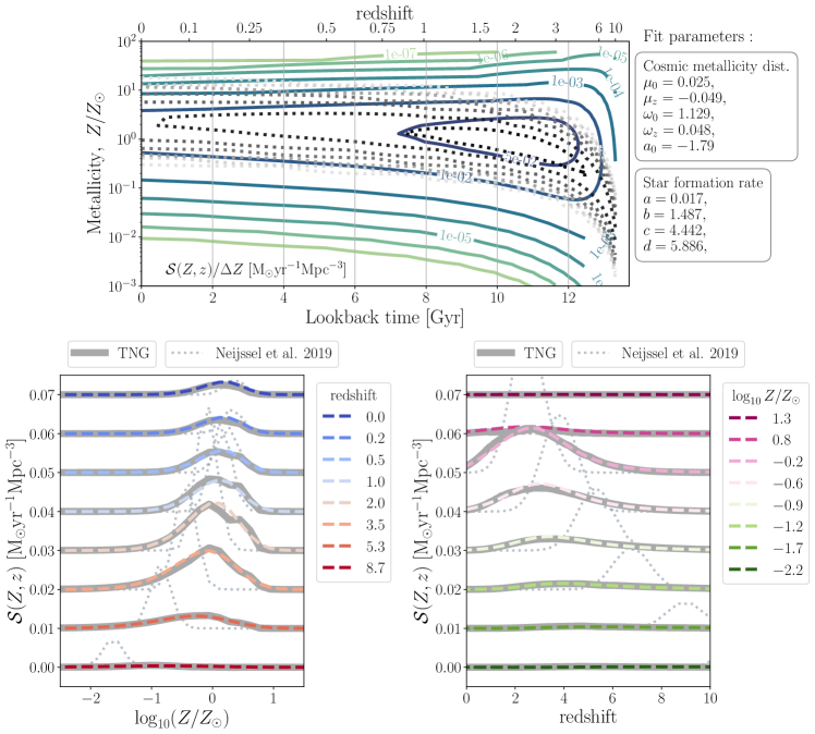
Figure 1: Our fiducial $\mathcal{S}(Z,z)$ model, adopting the best fitting parameters (listed on the top right) to fit the TNG100 simulations. The top panel shows the full two dimensional $\mathcal{S}(Z,z)$ linear in time. Contours range from $10^{-7}-10^{-2}\rm{M}_{\odot}\,\rm{yr}^{-1}\,\rm{Mpc}^{-3}$. The bottom left (right) panel shows slices of the distribution in redshift (metallicity). Each slice is displaced by 0.01$\rm{M}_{\odot}\,\rm{yr}^{-1}\,\rm{Mpc}^{-3}$ (note the linear scale of $\mathcal{S}(Z,z)$ in the bottom panel). We show the TNG100 simulation data with thick gray lines. For comparison, we also show the phenomenological model from Neijssel et al. (2019) in all panels with grey dotted lines. The bottom panels show that our analytical model adequately captures the shape of the $\mathcal{S}(Z,z)$ from TNG100.

Our best fitting parameters are listed in Table 1. With these fit parameters, $\chi^{2}(z_{j})$ is smaller than $2\cdot 10^{-4}$ at any given redshift. To evaluate our fit, we show the absolute residuals and relative errors in Appendix A. We will refer to the $\mathcal{S}(Z,z)$ with the parameters listed in Table 1 as our fiducial model.

Table 1: Best fitting parameters for our $\mathcal{S}(Z,z)$ fit to TNG100 data.

dP/dZ	description	best fit	SFRD(z)	best fit
			$\rm{M}_{\odot}\,\rm{yr}^{-1}\,\rm{Mpc}^{-3}$
$\mu_{0}$	mean metallicity at $z=0$	$0.025\pm 0.036$	$a$	$0.02\pm 0.072$
$\mu_{z}$	$z$-dependence of the mean	$-0.049\pm 0.006$	$b$	$1.48\pm 0.002$
$\alpha$	shape (skewness)	$-1.778\pm 0.002$	$c$	$4.44\pm 0.001$
$\omega_{0}$	scale at $z=0$	$1.122\pm 0.001$	$d$	$5.90\pm 0.002$
$\omega_{z}$	$z$-dependence of the scale	$0.049\pm 0.009$

In Figure 1 we show our fiducial model at different redshifts and metallicities. We also show the overall star-formation rate density $\mathrm{SFRD}(z)$ in Figure 2. In general, our analytical model captures the metallicity-dependent cosmic star formation history in the TNG100 simulations well (bottom panels of Figure 1). The skewed-log normal metallicity distribution is able to reproduce the overall behaviour that is observed in TNG100 (bottom left panel, but cf. Pakmor et al., 2022, for an in-depth discussion of low metallicity star formation in the TNG50 simulation). Only minor features like the additional bump just above $\log_{10}(Z)=-2$ at redshift 2 are missed. However, for our purposes, it is more important to prioritise fitting the large scale trends, while we are not so interested in smaller scale fluctuations.

Adopting a skewed-lognormal metallicity distribution allows for a tail of low metallicity star formation out to low redshifts. To emphasise the difference between a skewed-lognormal and a symmetric lognormal distribution, we show the phenomenological model from Neijssel et al. (2019) in dotted grey. Their model falls within the family of functions that is encompassed by our model described in Section 2, but we note that their model is distinctly different.

Although our model preforms well at reproducing the large scale trends seen in TNG, we acknowledge that more complex features as suggested by some observational studies could be missed. One example is that the $\mathrm{SFRD}(z)$ shape we adopt from Madau & Dickinson (2014) does not account for starburst galaxies (see discussion in Chruślińska et al., 2021). Moreover, our model cannot capture inflection points in the mean metallicity, because we assume both $\mu_{0}$ and $\mu_{z}$ are constants with redshift (equation 7). Contrarily, Chruślińska & Nelemans (2019) find an upturn in the amount of low metallicity star formation above $z=4$ if the power law of the GSMF is allowed to evolve with redshift. Hence, although our model is more broadly applicable than previous models, in it’s current form, it does not capture the complete range of observationally-allowed variations. Incorporating more complex functional forms for our the mean metallicity could possibly capture such behaviour, but this analysis is beyond the scope of this paper.

4 Application: systematic variations of $\mathcal{S}(Z,z)$ and the effect on the mass distribution of merging BBHs

We will now demonstrate the application of our analytical model by systematically varying the parameters in our fiducial $\mathcal{S}(Z,z)$ model, and investigate their effect on the local mass distribution of BBH mergers originating from isolated binaries.

We use the publicly available rapid binary population synthesis simulations presented in van Son et al. (2022b). These simulations were run using version v02.26.03 of the open source COMPAS suite (Riley et al., 2022). COMPAS is based on algorithms that model the evolution of massive binary stars following Hurley et al. (2000, 2002) using detailed evolutionary models by Pols et al. (1998). In particular, we use the simulations behind Figure 1 from van Son et al. (2022b), and we refer the reader to their methods section for a detailed description of the adopted physics parameters and assumptions. Metallicities of each binary system were sampled from a smooth probability distribution to avoid artificial peaks in the BH mass distribution (e.g. Dominik et al., 2015; Kummer, 2020). These simulations provide us with an estimate of the yield of BBH mergers per unit of star-forming mass and metallicity.

We combine the aforementioned yield with variations of the fiducial $\mathcal{S}(Z,z)$ model described in this work. By integrating over cosmic history, we obtain the local merger rates of BBH systems, which allow us to construct the distribution of source properties at every redshift. We use the cosmic integration scheme that is part of the publicly available COMPAS suite, which includes the $\mathcal{S}(Z,z)$ model described in this work. The details of this framework are described in Neijssel et al. (2019), but also in van Son et al. (2022a), where more similar settings to this work are used.

4.1 Determining reasonable variations of $\mathcal{S}(Z,z)$

We consider variations in both the shape of the cosmic metallicity density distribution $\mathrm{dP/dZ}(Z,z)$, and the shape of the overall star-formation rate density, $\mathrm{SFRD}(z)$. To determine the range that is reasonably allowed by observations, we compare our variations to the observation-based $\mathcal{S}(Z,z)$ models described in Chruślińska et al. (2021). An overview of the explored variations is shown in Table 2. Below we explain how we arrive at these values.

Table 2: Variations on $\mathcal{S}(Z,z)$. For every variation, we either swap the value of an individual $\mathrm{dP/dZ}(Z,z)$ parameter, or exchange the set of four $\mathrm{SFRD}(z)$ parameters, and replace them by the the min/max values listed here. All other parameters are kept fixed at their fiducial value.

	min	fiducial	max
$\mathrm{dP/dZ}(Z,z)$
$\mu_{0}$	0.007	$0.025$	0.035
$\mu_{z}$	0.0	$-0.049$	-0.5
$\alpha$	-6.0	$-1.778$	0.0
$\omega_{0}$	0.7	$1.125$	2.0
$\omega_{z}$	0.0	$0.048$	0.1
$\mathrm{SFRD}(z)$
($a$,$b$ …	($0.01$, $2.60$	($0.02$, $1.48$	($0.03$, $2.6$
… $c$,$d$)	$3.20$, $6.20$)	$4.44$, $5.90$)	$3.3$, $5.9$)

For the cosmic metallicity density distribution, we vary every parameter that determines the shape of $\mathrm{dP/dZ}(Z,z)$ independently (three left-most columns of Table 1, and top of Table 2 ), while keeping all other parameters fixed at their fiducial value. For each variation, we inspect the fraction of stellar mass that is formed at low-metallicity ($Z<0.1Z_{\odot}$) versus the fraction of stellar mass that is formed at high-metallicity ($Z>Z_{\odot}$), for all star formation that occurred below a certain threshold redshift. We compare this to the models from Chruślińska et al. (2021) in Figure 6 in Appendix B. We have chosen our variations such that they span a reasonable range of cosmic metallicity density distributions as allowed by observation-based and cosmological simulations-based models. We use the models 214-f14SB-BiC_FMR270_FOH_z_dM.dat, and 302-f14SB-Boco_FMR270_FOH_z_dM.dat from Chruślińska et al. (2021) as a representation of a very low and high metallicity star formation realisation respectively. These models are the low and high metallicity extreme under their fiducial SFR–metallicity correlation, and so we will refer to them as Chr21_lowZ and Chr21_highZ respectively from hereon. The difference between these models lies in the assumptions in the underlying empirical galaxy relations. In general, low-mass galaxies contribute to low-metallicity star formation and shift the peak of $\mathcal{S}(Z,z)$ to lower metallicities. Chr21_lowZ is characterised by a star formation–galaxy mass relation that is flat at high galaxy masses (reducing the star formation rate for the highest-mass galaxies), a galaxy stellar mass function that evolves with redshift (predicting an increasing number density of low-mass galaxies), and a local galaxy mass-metallicity relation as in Pettini & Pagel (2004). This model further approximates the contribution of starburst galaxies following Bisigello et al. (2018) and Caputi et al. (2017). Assuming that starburst galaxies follow the empirical fundamental metallicity relation (leading to anti-correlation between the SFR and metallicity), their inclusion tends to shift the peak of $\mathcal{S}(Z,z)$ to lower metallicities and broadens the low-metallicity part of the distribution.

On the other hand, Chr21_highZ assumes the star formation–galaxy mass relation does not flatten towards higher galaxy masses, a galaxy stellar mass function where the slope for the low-mass end is constant over redshift, and a local galaxy mass-metallicity relation following Kobulnicky & Kewley (2004). Lastly, this model adopts the starburst prescription from Boco et al. (2021), which produces results that are similar to models without starburst galaxies.

For every variation of our model, we inspect both the full $\mathcal{S}(Z,z)$ and slices at redshifts $z=0,0.5,3.0$ and $6$ by eye. At each slice we compare our model variation to Chr21_lowZ and Chr21_highZ, and ensure that none of our variations significantly exceeds these extremes in $\mathcal{S}(Z,z)$. This also serves as a sanity check for the overall star-formation rate density.

We also consider two variations of the overall star-formation rate density, $\mathrm{SFRD}(z)$, where we keep the metallicity distribution $\mathrm{dP/dZ}(Z,z)$ fixed, but vary all four $\mathrm{SFRD}(z)$ parameters at once (right two columns of Table 1, and bottom of Table 2). We use Figure 11 from Chruślińska et al. (2021) to determine approximate upper and lower bounds to the overall star-formation rate density. We choose Madau & Fragos (2017) as an approximation of the lower limit. For the upper limit, we use the upper edge of models that adopt starbursts following Bisigello et al. (2018) and Caputi et al. (2017) (SB: B18/C17), combined with a non-evolving low-mass end of the galaxy stellar mass function (shown as a thick brown line in Fig. 11 of Chruślińska et al., 2021, and described in their table B1). To approximate these models, we fit equation 12 by eye to the broken power law description of this model as presented in appendix B1 of Chruślińska et al. (2021). We show all $\mathrm{SFRD}(z)$ variations in Figure 2.

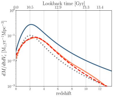
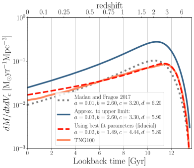
Figure 2: Comparison of several overall star-formation rate densities, $\mathrm{SFRD}(z)$, with redshift (left panel) and with lookback time (right panel). The solid orange and dashed red lines respectively show the star formation data from TNG100 and our corresponding fit adopting eq. 12 (fiducial model). The dotted gray and solid blue lines are variations of eq. 12 used to approximate the lower and upper edge of possible star-formation histories. The dotted gray line shows the model from Madau & Fragos (2017), while the solid blue line mimics the behaviour of the powerlaw-fit to the SB: B18/C17 variations with a non-evolving low-mass end of the galaxy stellar mass function from Chruślińska et al. (2021).

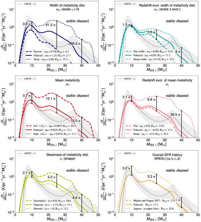
Figure 3: The primary mass distribution of merging BBH systems from the stable mass transfer channel for several variations in $\mathcal{S}(Z,z)$. The first five panels show variations of the cosmic metallicity density distribution $\mathrm{dP/dZ}(Z,z)$, eq. 11, (parameters listed in the first three columns of Table 1), where we vary one parameter at a time while keeping the rest fixed at their fiducial value. The bottom right panel shows variations in the magnitude of the star formation rate with redshift; i.e. $\mathrm{SFRD}(z)$. For the latter we vary the four fiducial parameters of $\mathrm{SFRD}(z)$ simultaneously (last two columns of Table 1). All panels are shown at a reference redshift of $z=0.2$, with the corresponding predicted BBH merger rate indicated in the legend. For reference, we show the power-law + peak model from Abbott et al. (2021b) in grey. We annotate the relative change in the rate at three reference masses: $10\rm{M}_{\odot}$, $25\rm{M}_{\odot}$ and $40\rm{M}_{\odot}$.

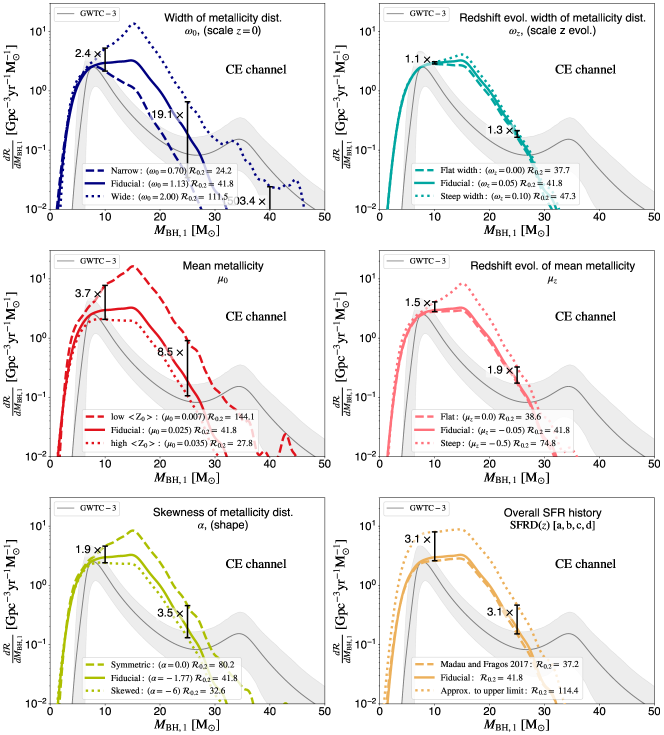
Figure 4: Same as Figure 3, but for the Common Envelope channel. These figures show that the low mass end of the primary mass distribution is least affected by the adopted $\mathcal{S}(Z,z)$. Moreover, the location of features in the mass distribution are robust against all explored variations.

4.2 The effect of the $\mathcal{S}(Z,z)$ on the primary masses of merging BBH

To isolate the effect of the $\mathcal{S}(Z,z)$ from the effects of different formation channels, we split the data from van Son et al. (2022a) between the stable mass transfer channel (e.g., van den Heuvel et al., 2017; Inayoshi et al., 2017; Bavera et al., 2021; Marchant et al., 2021; Gallegos-Garcia et al., 2021; van Son et al., 2022a), and the ‘classical’ common-envelope channel (or CE channel, e.g.,  Belczynski et al., 2007; Postnov & Yungelson, 2014; Belczynski et al., 2016; Vigna-Gómez et al., 2018). These channels are distinguished based on whether the binary system has experienced a common envelope phase (CE channel) or only stable mass transfer (stable channel in short from now on).

In Figures 3 and 4, we show the resulting primary mass distribution of merging BBHs from the stable channel and CE channel respectively. The primary (secondary) component refers to the more (less) massive component of merging BBHs. Each panel varies one aspect of the $\mathcal{S}(Z,z)$. In the first five panels of Figures 3 and 4, we vary one of the parameters that determine the shape of the probability density distribution of metallicities, while keeping all other values fixed at their fiducial values. In the last panel of Figures 3 and 4, we vary the shape of the overall star-formation rate densities, $\mathrm{SFRD}(z)$, to one of the variations shown in Figure 2, while keeping the probability density distribution of metallicities fixed.

The first thing we note is that the location of the features in the primary mass distribution are robust against variations in $\mathcal{S}(Z,z)$. For the stable channel, two features are visible in all variations: a peak at $\,M_{\rm BH,1}\approx 9\rm{M}_{\odot}$ and a bump at $\,M_{\rm BH,1}\approx 22\rm{M}_{\odot}$. Two more features are visible in at the high mass end for almost all $\mathcal{S}(Z,z)$; a knee at $\,M_{\rm BH,1}\approx 35\rm{M}_{\odot}$ and another bump at $\,M_{\rm BH,1}\approx 45\rm{M}_{\odot}$. Although the locations of these features are constant, the features themselves can disappear for variations that suppress the rate of high mass BHs (e.g., dashed lines in the top panels of Fig. 3). Similarly, the CE channel displays a kink in the distribution at about $9\rm{M}_{\odot}$, and a peak at approximately $\,M_{\rm BH,1}\approx 17\rm{M}_{\odot}$ for all variations. The latter peak is the global peak of the mass distribution in almost all variations.

The finding that the locations of features in the mass distribution do not change for different $\mathcal{S}(Z,z)$ is consistent with earlier work. Recent work by Chruślińska (2022) showed that, when comparing two very different models of $\mathcal{S}(Z,z)$ (their Figure 5), the location of the peaks remains the same, even though the normalisation between the two BBH merger rates is completely different. Furthermore, Broekgaarden et al. (2021) show the probability distribution of chirp masses for BBHs in their Fig. 4. Although features can disappear when the $\mathcal{S}(Z,z)$ prohibits the formation of certain (typically higher) mass BHs, the location of features remains the same. This implies that the locations of features in the mass distribution of BBHs are determined by the formation channel and its underlying stellar and binary physics. The locations of features could therefore serve as sign posts of the underlying physics.

Second, we see that the low mass end of the primary mass distribution is relatively robust against variations in $\mathcal{S}(Z,z)$. To quantify this, we annotate the ratio between the maximum and minimum rate at three reference masses; $\,M_{\rm BH,1}$ = $10,25$, and $40\rm{M}_{\odot}$. At $\,M_{\rm BH,1}=10\rm{M}_{\odot}$, we find that the rate changes by at most a factor of about 3.7 for the stable channel, and at most about a factor of 3.8 for the CE channel. On the other hand, the change in rate at $\,M_{\rm BH,1}=40\rm{M}_{\odot}$ can be as high as a factor of about 200 and 150 for the stable and CE channels, respectively. The lowest mass BHs are least affected by the $\mathcal{S}(Z,z)$ because they can be formed from all metallicities above $Z\gtrsim 10^{-3}$ (see e.g., Figures 7 and 13 from van Son et al., 2022a). The rate of star formation at metallicities above $\gtrsim 10^{-3}$ is observationally relatively well constrained for redshifts below $0.5$ (which comprises the past $5\,\rm{Gyr}$ of star formation). This is reflected in the top panel of Figure 6: all models show that $10\%$ or less of the stellar mass was formed at a metallicity below $Z/10\approx 0.0014$, or in other words, about $90\%$ or more of the stellar mass was formed at a metallicity above $Z/10$. Hence the lowest mass BHs derive from the least uncertain parts of the $\mathcal{S}(Z,z)$. The low-mass end of the mass distribution of merging double compact objects will also provide a particularly powerful cosmological constraint in the era of third generation gravitational wave telescopes (María Ezquiaga & Holz, 2022). Our finding that the low mass end is more robust against variations in $\mathcal{S}(Z,z)$ supports this claim.

Parameter variations that affect shape of $\mathcal{S}(Z,z)$ at low redshift primarily change the normalisation of the mass distribution. This is the case for variations of the width of the cosmic metallicity density distribution at $z=0$ ($\omega_{0}$), the mean metallicity of the cosmic metallicity density distribution at $z=0$ ($\mu_{0}$), and the skewness of the cosmic metallicity density distribution ($\alpha$, left columns of Figures 3 and 4). To emphasise this point, we annotate the total BBH merger rate at redshift 0.2, $\mathcal{R}_{0.2}$, in the legends of Figures 3 and 4 (0.2 is the redshift where the observations are best constrained Abbott et al. 2021b). Variations that increase the amount of star formation at low metallicity (i.e. for a low mean metallicity $\mu_{0}=0.007$ and a wide metallicity distribution $\omega_{0}=2.0$ ) increase the predicted BBH merger rate. This is consistent with other work that finds merging BBHs form more efficiently at low metallicities (e.g. Belczynski et al., 2010; Stevenson et al., 2017; Mapelli et al., 2017; Chruślińska et al., 2019; Broekgaarden et al., 2021). A more skewed cosmic metallicity density distribution pushes the peak of the distribution to higher metallicities and thus forms more stars at high metallicity when compared to a symmetric distribution. Hence, the local rate of BBH mergers is lower for the skewed distribution ($\alpha=-6$) with respect to the symmetric variation ($\alpha=0.0$).

Changing the overall star-formation rate density ($\mathrm{SFRD}(z)$, bottom right panels of Figures 3 and 4) also affects the normalisation of the mass distribution, but has a smaller effect than the width and the mean of the cosmic metallicity density distribution at $z=0$ ($\omega_{0}$ and $\mu_{0}$). This underlines the importance of the amount of low-metallicity star formation (e.g., Chruślińska, 2022), and is furthermore in line with findings from Tang et al. (2020). As discussed in Section 4.1, we use Madau & Fragos (2017) and the solid blue line in Figure 2 as an approximate lower and upper bound to the $\mathrm{SFRD}(z)$ respectively. The overall cosmic star formation rate density from Madau & Fragos (2017) is very similar to our fiducial model (Figure 2), and the differences between the resulting mass distributions are correspondingly small. Our approximation of the upper limit to the allowed $\mathrm{SFRD}(z)$ leads to an overall increase of the BBH merger rate by a factor of about 3.

Parameters that change the evolution of the metallicity distribution $\mathrm{dP/dZ}(Z,z)$ with redshift, such as the redshift dependence of the with and mean; $\omega_{z}$ and $\mu_{z}$ (top right and centre right panels of Figures 3 and 4) primarily affect the high mass end of the stable channel. We understand this as an effect of the different delay time distributions for both formation channels. Since both, $\omega_{z}$ and $\mu_{z}$ influence the amount of low metallicity stellar mass formed at high redshifts they will mostly affect systems with longer delay times. The stable channel has been shown to produce more high mass BHs with longer delay times when compared to the CE channel (van Son et al., 2022a; Briel et al., 2022b). Hence we find these variations affect the slope of the high mass end of the BBH mass distribution for the stable channel, while they have a relatively small impact on the CE channel.

5 Discussion & Summary

We present a flexible analytic expression for the metallicity-dependent cosmic star formation history, $\mathcal{S}(Z,z)$ (equations 1, 11 and 12). An analytical expression allows for controlled experiments of the effect of $\mathcal{S}(Z,z)$ on dependent values, such as the rate and mass distribution of merging BBHs. The model presented in this work adopts a skewed-lognormal for the distribution of metallicities at every redshift ($\mathrm{dP/dZ}(Z,z)$).

The model can capture the general behaviour of cosmological simulations, such as TNG100

Our analytical expression for $\mathcal{S}(Z,z)$ is composed of a cosmic metallicity density distribution that is determined by a mean, scale and skewness and their redshift dependence, as well as parameters governing the overall star-formation rate density. We fit our analytical expression for $\mathcal{S}(Z,z)$ to the star-forming gas in the TNG100 simulation, and provide the best fit parameters in Table 1. We show that our model captures the shape and general behaviour of the cosmological simulations well (Figure 1). Although our model is more broadly applicable than previous models, we acknowledge that it does not capture the complete range of observationally-allowed variations in it’s current form. Incorporating more complex functions for the redshift evolution of the metallicity could solve this issue, but this is left for future research.

The model allows for a controlled experiment on the effect of $\mathcal{S}(Z,z)$ on the local distribution of merging BBH

As an example, we use our model to calculate the local rate and mass distribution of the more massive components from merging BBHs ($\,M_{\rm BH,1}$) in Figures 3 and 4. We systematically vary all five parameters that shape the cosmic metallicity density distribution, and explore two additional variations of the overall star-formation rate density $\mathrm{SFRD}(z)$. Our main findings are as follows:

• The locations of features in the distribution of primary BH masses are robust against variations in $\mathcal{S}(Z,z)$. The location of features in the mass distribution of BHs could thus be used as sign posts of their formation channel.

• For all variations, the low mass end of the mass distribution is least influenced by changes in the $\mathcal{S}(Z,z)$. This is because the lowest mass BHs can be formed from all metallicities above $Z~{}\gtrsim~{}10^{-3}$, for which the star formation rate is relatively well constrained in the recent Universe. This suggests that the lower end of the BH mass distribution (component masses of $\leq 15\rm{M}_{\odot}$) is potentially very powerful for constraining the physics of the formation channels, irrespective of the cosmic star formation rate uncertainties.

• The metallicity distribution of star formation at low redshift primarily impacts the normalisation of the BBH merger rate. Changing the overall star-formation rate density, $\mathrm{SFRD}(z)$ also affects the rate, but to a lesser degree. This shows that low-metallicity star formation at low redshifts dominates the overall normalisation of the BBH merger rate.

• Parameters that influence the redshift evolution of the mean and the width of the metallicity distribution affect the slope of the high mass end of the primary BH mass distribution for the stable channel. This reflects the longer delay times of the stable channel with respect to the CE channel.

The flexibility of the model presented in this work can capture the large uncertainties that remain in the shape and normalisation of the metallicity-dependent cosmic star formation history. Our hope is that this expression will provide a useful starting point for making predictions and comparisons with observations.

Software and Data

All code associated to reproduce the data and plots in this paper is publicly available at https://github.com/LiekeVanSon/SFRD_fit. The data used in this work is available on Zenodo under an open-source Creative Commons Attribution license at https://zenodo.org/record/7612755 (catalog 10.5281/zenodo.7612755). All observationally constrained models of the $\mathcal{S}(Z,z)$ from Chruślińska et al. (2021) can be found online at: https://ftp.science.ru.nl/astro/mchruslinska/Chruslinska_et_al_2021/.

This research has made use of GW data provided by the Gravitational Wave Open Science Center (https://www.gw-openscience.org/), a service of LIGO Laboratory, the LIGO Scientific Collaboration and the Virgo Collaboration. Further software used in this work: Python (Van Rossum & Drake, 2009), Astropy (Astropy Collaboration et al., 2013, 2018) Matplotlib (Hunter, 2007), NumPy (Harris et al., 2020), SciPy (Virtanen et al., 2020), ipython$/$jupyter (Perez & Granger, 2007; Kluyver et al., 2016), Seaborn (Waskom, 2021) and hdf5 (Collette et al., 2019).

Appendix A Evaluating our fit; the squared residuals

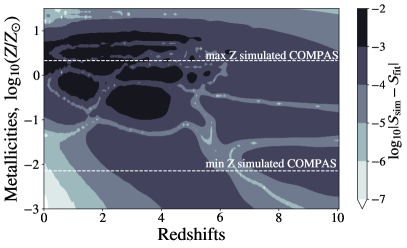
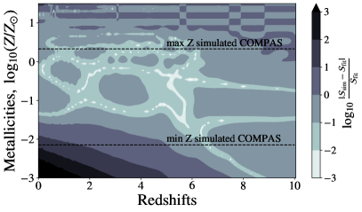
Figure 5: $\log$ of the residuals (left), and $\log$ of the relative error (right) between the TNG100 data and our best-fitting model. We show the minimum and maximum metallicity used in COMPAS simulations with dashed lines in each plot.

In the left panel of Figure 5, we show the $\log$ of the absolute residuals. The square of the residuals is used in the cost function, equation 14, to optimise our fit. We observe that the maximum residuals appear near the peak of star formation at high metallicities. The log of the relative errors (defined as $\frac{\lvert\mathcal{S}{\rm sim}-\mathcal{S}{\rm fit}\rvert}{\mathcal{S}_{\rm fit}}$), is shown in the right-hand panel of Figure 5. The relative errors generally exhibit an opposite trend with respect to the residuals. The relative errors are largest in regions of very low-metallicity star formation at low redshift. This occurs due to the very low star-formation rate in this regime (of the order $10^{-8}\rm{M}_{\odot}\,\rm{yr}^{-1}\,\rm{Mpc}^{-3}$ for the TNG simulations and $10^{-11}\rm{M}_{\odot}\,\rm{yr}^{-1}\,\rm{Mpc}^{-3}$ in our model fit). Another regime where the relative error becomes large is at very high metallicities (about 10 times $Z_{\odot}$). This is because in this regime, the TNG data is very sparse and contains regions where the rate abruptly drops to zero. To avoid sharp features in the data, we use interpolated TNG data to produce the fit. We note that we chose to minimise the squared residuals (which is similar to minimising the mean squared error) in favour of minimising, for example, the relative error, to prevent overfitting such regions of very low star-formation rate. For the illustration purposes in this work, we are most interested in closely fitting the $\mathcal{S}(Z,z)$ between the minimum ($10^{-4}$) and maximum ($0.03$) metallicities that can be simulated with COMPAS. For applications that focus on extremely low ($<0.01Z_{\odot}$) or extremely high ($\sim 10\times Z_{\odot}$) metallicity star formation, a different cost function would be more appropriate.

Appendix B Determining reasonable variations of the $\mathcal{S}(Z,z)$

To determine reasonable variations of our fiducial model for $\mathcal{S}(Z,z)$, we compute the fraction of low and high metallicity stellar mass formed for redshifts below $z<0.5$, $z<3.0$ and $z<10$. We show the results in Figure 6, which is an adaptation of Fig. 2 in Pakmor et al. (2022), which in turn builds on Fig. 9 from Chruślińska & Nelemans (2019).

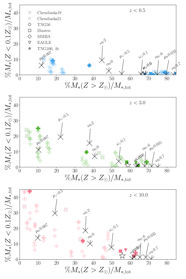
Figure 6: Percentage of stellar mass formed at low metallicity ($Z<0.1\rm{Z_{\odot}}$) , versus high metallicity ($Z>\rm{Z_{\odot}}$) for all star formation below a certain threshold redshift: $z<0.5$ (top), $z<3.0$ (middle) and $z<10$ (bottom). Data from observation-based variations are shown with semi-transparent thick crosses, (Chruślińska & Nelemans, 2019) and semi-transparent thick plus signs (Chruślińska et al., 2021), the low- and high-metallicity extremes are indicated with opaque symbols. For data from cosmological simulations, we follow Pakmor et al. (2022) and show Illustris (Vogelsberger et al., 2014, squares), Simba (Davé et al., 2019, diamonds), EAGLE (Schaye et al., 2015, triangles), TNG50 and TNG100 (Springel et al., 2018, filled and open circles respectively). Black thin crosses display variations of the cosmic metallicity density distribution that is part of our fiducial $\mathcal{S}(Z,z)$. The parameter that is varied with respect to the fiducial and its new value are annotated. This shows that our $\mathcal{S}(Z,z)$ variations span the range of reasonable cosmic metallicity density distributions as determined by observation-based and cosmological simulations-based models.

References

- Abbott et al. (2016) Abbott, B. P., Abbott, R., Abbott, T. D., et al. 2016, ApJ, 818, L22, doi: 10.3847/2041-8205/818/2/L22
- Abbott et al. (2018) Abbott, B. P., et al. 2018, Phys. Rev. https://arxiv.org/abs/1811.12907
- Abbott et al. (2020) Abbott, R., Abbott, T. D., Abraham, S., et al. 2020, arXiv e-prints, arXiv:2010.14527. https://arxiv.org/abs/2010.14527
- Abbott et al. (2021a) Abbott, R., Abbott, T. D., Acernese, F., et al. 2021a, arXiv e-prints, arXiv:2111.03606. https://arxiv.org/abs/2111.03606
- Abbott et al. (2021b) —. 2021b, arXiv e-prints, arXiv:2111.03634. https://arxiv.org/abs/2111.03634
- Astropy Collaboration et al. (2013) Astropy Collaboration, Robitaille, T. P., Tollerud, E. J., et al. 2013, A&A, 558, A33, doi: 10.1051/0004-6361/201322068
- Astropy Collaboration et al. (2018) Astropy Collaboration, Price-Whelan, A. M., Sipőcz, B. M., et al. 2018, AJ, 156, 123, doi: 10.3847/1538-3881/aabc4f
- Bavera et al. (2021) Bavera, S. S., Fragos, T., Zevin, M., et al. 2021, A&A, 647, A153, doi: 10.1051/0004-6361/202039804
- Bavera et al. (2022) Bavera, S. S., Fragos, T., Zapartas, E., et al. 2022, A&A, 657, L8, doi: 10.1051/0004-6361/202141979
- Belczynski et al. (2010) Belczynski, K., Bulik, T., Fryer, C. L., et al. 2010, ApJ, 714, 1217, doi: 10.1088/0004-637X/714/2/1217
- Belczynski et al. (2016) Belczynski, K., Holz, D. E., Bulik, T., & O’Shaughnessy, R. 2016, Nature, 534, 512, doi: 10.1038/nature18322
- Belczynski et al. (2007) Belczynski, K., Taam, R. E., Kalogera, V., Rasio, F. A., & Bulik, T. 2007, ApJ, 662, 504, doi: 10.1086/513562
- Bisigello et al. (2018) Bisigello, L., Caputi, K. I., Grogin, N., & Koekemoer, A. 2018, A&A, 609, A82, doi: 10.1051/0004-6361/20173139910.48550/arXiv.1706.06154
- Boco et al. (2021) Boco, L., Lapi, A., Chruslinska, M., et al. 2021, ApJ, 907, 110, doi: 10.3847/1538-4357/abd3a0
- Briel et al. (2022a) Briel, M. M., Eldridge, J. J., Stanway, E. R., Stevance, H. F., & Chrimes, A. A. 2022a, MNRAS, 514, 1315, doi: 10.1093/mnras/stac1100
- Briel et al. (2022b) Briel, M. M., Stevance, H. F., & Eldridge, J. J. 2022b, arXiv e-prints, arXiv:2206.13842. https://arxiv.org/abs/2206.13842
- Broekgaarden et al. (2021) Broekgaarden, F. S., Berger, E., Stevenson, S., et al. 2021, arXiv e-prints, arXiv:2112.05763. https://arxiv.org/abs/2112.05763
- Caputi et al. (2017) Caputi, K. I., Deshmukh, S., Ashby, M. L. N., et al. 2017, ApJ, 849, 45, doi: 10.3847/1538-4357/aa901e10.48550/arXiv.1705.06179
- Chruślińska (2022) Chruślińska, M. 2022, arXiv e-prints, arXiv:2206.10622. https://arxiv.org/abs/2206.10622
- Chruślińska & Nelemans (2019) Chruślińska, M., & Nelemans, G. 2019, MNRAS, 488, 5300, doi: 10.1093/mnras/stz2057
- Chruślińska et al. (2019) Chruślińska, M., Nelemans, G., & Belczynski, K. 2019, MNRAS, 482, 5012, doi: 10.1093/mnras/sty3087
- Chruślińska et al. (2021) Chruślińska, M., Nelemans, G., Boco, L., & Lapi, A. 2021, MNRAS, 508, 4994, doi: 10.1093/mnras/stab2690
- Collette et al. (2019) Collette, A., Caswell, T. A., Tocknell, J., et al. 2019, h5py/h5py: 2.10.0, 2.10.0, Zenodo, Zenodo, doi: 10.5281/zenodo.3401726
- Cresci et al. (2019) Cresci, G., Mannucci, F., & Curti, M. 2019, A&A, 627, A42, doi: 10.1051/0004-6361/201834637
- Davé et al. (2019) Davé, R., Anglés-Alcázar, D., Narayanan, D., et al. 2019, MNRAS, 486, 2827, doi: 10.1093/mnras/stz937
- Dominik et al. (2013) Dominik, M., Belczynski, K., Fryer, C., et al. 2013, ApJ, 779, 72, doi: 10.1088/0004-637X/779/1/72
- Dominik et al. (2015) Dominik, M., Berti, E., O’Shaughnessy, R., et al. 2015, ApJ, 806, 263, doi: 10.1088/0004-637X/806/2/263
- Doughty & Finlator (2021) Doughty, C., & Finlator, K. 2021, MNRAS, 505, 2207, doi: 10.1093/mnras/stab1448
- Dray et al. (2003) Dray, L. M., Tout, C. A., Karakas, A. I., & Lattanzio, J. C. 2003, MNRAS, 338, 973, doi: 10.1046/j.1365-8711.2003.06142.x
- Farmer et al. (2021) Farmer, R., Laplace, E., de Mink, S. E., & Justham, S. 2021, ApJ, 923, 214, doi: 10.3847/1538-4357/ac2f44
- Fruchter et al. (2006) Fruchter, A. S., Levan, A. J., Strolger, L., et al. 2006, Nature, 441, 463, doi: 10.1038/nature04787
- Gallegos-Garcia et al. (2021) Gallegos-Garcia, M., Berry, C. P. L., Marchant, P., & Kalogera, V. 2021, arXiv e-prints, arXiv:2107.05702. https://arxiv.org/abs/2107.05702
- Goswami et al. (2022) Goswami, S., Silva, L., Bressan, A., et al. 2022, A&A, 663, A1, doi: 10.1051/0004-6361/202142031
- Götberg et al. (2020) Götberg, Y., de Mink, S. E., McQuinn, M., et al. 2020, A&A, 634, A134, doi: 10.1051/0004-6361/201936669
- Harris et al. (2020) Harris, C. R., Millman, K. J., van der Walt, S. J., et al. 2020, Nature, 585, 357–362, doi: 10.1038/s41586-020-2649-2
- Hemler et al. (2021) Hemler, Z. S., Torrey, P., Qi, J., et al. 2021, MNRAS, 506, 3024, doi: 10.1093/mnras/stab1803
- Hunter (2007) Hunter, J. D. 2007, Computing in Science and Engineering, 9, 90, doi: 10.1109/MCSE.2007.55
- Hurley et al. (2000) Hurley, J. R., Pols, O. R., & Tout, C. A. 2000, MNRAS, 315, 543, doi: 10.1046/j.1365-8711.2000.03426.x
- Hurley et al. (2002) Hurley, J. R., Tout, C. A., & Pols, O. R. 2002, MNRAS, 329, 897, doi: 10.1046/j.1365-8711.2002.05038.x
- Inayoshi et al. (2017) Inayoshi, K., Hirai, R., Kinugawa, T., & Hotokezaka, K. 2017, MNRAS, 468, 5020, doi: 10.1093/mnras/stx757
- Kennicutt (1989) Kennicutt, Robert C., J. 1989, ApJ, 344, 685, doi: 10.1086/167834
- Kewley & Ellison (2008) Kewley, L. J., & Ellison, S. L. 2008, ApJ, 681, 1183, doi: 10.1086/587500
- Kluyver et al. (2016) Kluyver, T., Ragan-Kelley, B., Pérez, F., et al. 2016, in ELPUB, 87–90
- Kobulnicky & Kewley (2004) Kobulnicky, H. A., & Kewley, L. J. 2004, ApJ, 617, 240, doi: 10.1086/42529910.48550/arXiv.astro-ph/0408128
- Kroupa (2001) Kroupa, P. 2001, MNRAS, 322, 231, doi: 10.1046/j.1365-8711.2001.04022.x
- Kummer (2020) Kummer, F. 2020, UvA Scripties
- Langer & Norman (2006) Langer, N., & Norman, C. A. 2006, ApJ, 638, L63, doi: 10.1086/500363
- Langer et al. (2007) Langer, N., Norman, C. A., de Koter, A., et al. 2007, A&A, 475, L19, doi: 10.1051/0004-6361:20078482
- Madau & Dickinson (2014) Madau, P., & Dickinson, M. 2014, ARA&A, 52, 415, doi: 10.1146/annurev-astro-081811-125615
- Madau & Fragos (2017) Madau, P., & Fragos, T. 2017, ApJ, 840, 39, doi: 10.3847/1538-4357/aa6af9
- Maiolino & Mannucci (2019) Maiolino, R., & Mannucci, F. 2019, A&A Rev., 27, 3, doi: 10.1007/s00159-018-0112-2
- Mapelli et al. (2017) Mapelli, M., Giacobbo, N., Ripamonti, E., & Spera, M. 2017, MNRAS, 472, 2422, doi: 10.1093/mnras/stx2123
- Marchant et al. (2021) Marchant, P., Pappas, K. M. W., Gallegos-Garcia, M., et al. 2021, arXiv e-prints, arXiv:2103.09243. https://arxiv.org/abs/2103.09243
- María Ezquiaga & Holz (2022) María Ezquiaga, J., & Holz, D. E. 2022, arXiv e-prints, arXiv:2202.08240. https://arxiv.org/abs/2202.08240
- Marinacci et al. (2018) Marinacci, F., Vogelsberger, M., Pakmor, R., et al. 2018, MNRAS, 480, 5113, doi: 10.1093/mnras/sty2206
- Naiman et al. (2018) Naiman, J. P., Pillepich, A., Springel, V., et al. 2018, MNRAS, 477, 1206, doi: 10.1093/mnras/sty618
- Neijssel et al. (2019) Neijssel, C. J., Vigna-Gómez, A., Stevenson, S., et al. 2019, MNRAS, 490, 3740, doi: 10.1093/mnras/stz2840
- Nelson et al. (2018) Nelson, D., Pillepich, A., Springel, V., et al. 2018, MNRAS, 475, 624, doi: 10.1093/mnras/stx3040
- Nelson et al. (2019a) —. 2019a, MNRAS, 490, 3234, doi: 10.1093/mnras/stz2306
- Nelson et al. (2019b) Nelson, D., Springel, V., Pillepich, A., et al. 2019b, Computational Astrophysics and Cosmology, 6, 2, doi: 10.1186/s40668-019-0028-x
- Nelson et al. (2021) Nelson, E. J., Tacchella, S., Diemer, B., et al. 2021, MNRAS, 508, 219, doi: 10.1093/mnras/stab2131
- Nocedal & Wright (2006) Nocedal, J., & Wright, S. 2006, Numerical optimization, 2nd edn., Springer series in operations research and financial engineering (New York, NY: Springer). http://gso.gbv.de/DB=2.1/CMD?ACT=SRCHA&SRT=YOP&IKT=1016&TRM=ppn+502988711&sourceid=fbw_bibsonomy
- O’Hagan & Leonard (1976) O’Hagan, A., & Leonard, T. 1976, Biometrika, 63, 201, doi: 10.1093/biomet/63.1.201
- Pakmor et al. (2022) Pakmor, R., Simpson, C. M., van de Voort, F., et al. 2022, MNRAS, 512, 3602, doi: 10.1093/mnras/stac717
- Perez & Granger (2007) Perez, F., & Granger, B. E. 2007, Computing in Science and Engineering, 9, 21, doi: 10.1109/MCSE.2007.53
- Pettini & Pagel (2004) Pettini, M., & Pagel, B. E. J. 2004, MNRAS, 348, L59, doi: 10.1111/j.1365-2966.2004.07591.x10.48550/arXiv.astro-ph/0401128
- Pillepich et al. (2018a) Pillepich, A., Nelson, D., Hernquist, L., et al. 2018a, MNRAS, 475, 648, doi: 10.1093/mnras/stx3112
- Pillepich et al. (2018b) Pillepich, A., Springel, V., Nelson, D., et al. 2018b, MNRAS, 473, 4077, doi: 10.1093/mnras/stx2656
- Pillepich et al. (2019) Pillepich, A., Nelson, D., Springel, V., et al. 2019, MNRAS, 490, 3196, doi: 10.1093/mnras/stz2338
- Planck Collaboration et al. (2020) Planck Collaboration, Aghanim, N., Akrami, Y., et al. 2020, A&A, 641, A6, doi: 10.1051/0004-6361/201833910
- Pols et al. (1998) Pols, O. R., Schröder, K.-P., Hurley, J. R., Tout, C. A., & Eggleton, P. P. 1998, MNRAS, 298, 525, doi: 10.1046/j.1365-8711.1998.01658.x
- Postnov & Yungelson (2014) Postnov, K. A., & Yungelson, L. R. 2014, Living Reviews in Relativity, 17, 3, doi: 10.12942/lrr-2014-3
- Riley et al. (2022) Riley, J., Agrawal, P., Barrett, J. W., et al. 2022, ApJS, 258, 34, doi: 10.3847/1538-4365/ac416c
- Sanders et al. (2022) Sanders, R. L., Shapley, A. E., Clarke, L., et al. 2022, arXiv e-prints, arXiv:2207.12430. https://arxiv.org/abs/2207.12430
- Santoliquido et al. (2021) Santoliquido, F., Mapelli, M., Giacobbo, N., Bouffanais, Y., & Artale, M. C. 2021, MNRAS, 502, 4877, doi: 10.1093/mnras/stab280
- Schaye et al. (2015) Schaye, J., Crain, R. A., Bower, R. G., et al. 2015, MNRAS, 446, 521, doi: 10.1093/mnras/stu2058
- Schmidt (1959) Schmidt, M. 1959, ApJ, 129, 243, doi: 10.1086/146614
- Smith (2014) Smith, N. 2014, ARA&A, 52, 487, doi: 10.1146/annurev-astro-081913-040025
- Springel et al. (2005) Springel, V., Di Matteo, T., & Hernquist, L. 2005, MNRAS, 361, 776, doi: 10.1111/j.1365-2966.2005.09238.x
- Springel & Hernquist (2003) Springel, V., & Hernquist, L. 2003, MNRAS, 339, 289, doi: 10.1046/j.1365-8711.2003.06206.x
- Springel et al. (2018) Springel, V., Pakmor, R., Pillepich, A., et al. 2018, MNRAS, 475, 676, doi: 10.1093/mnras/stx3304
- Stevenson et al. (2017) Stevenson, S., Vigna-Gómez, A., Mandel, I., et al. 2017, Nature Communications, 8, 14906, doi: 10.1038/ncomms14906
- Tang et al. (2020) Tang, P. N., Eldridge, J. J., Stanway, E. R., & Bray, J. C. 2020, MNRAS, 493, L6, doi: 10.1093/mnrasl/slz183
- Torrey et al. (2019) Torrey, P., Vogelsberger, M., Marinacci, F., et al. 2019, MNRAS, 484, 5587, doi: 10.1093/mnras/stz243
- van den Heuvel et al. (2017) van den Heuvel, E. P. J., Portegies Zwart, S. F., & de Mink, S. E. 2017, MNRAS, 471, 4256, doi: 10.1093/mnras/stx1430
- Van Rossum & Drake (2009) Van Rossum, G., & Drake, F. L. 2009, Python 3 Reference Manual (Scotts Valley, CA: CreateSpace)
- van Son et al. (2022a) van Son, L. A. C., de Mink, S. E., Callister, T., et al. 2022a, ApJ, 931, 17, doi: 10.3847/1538-4357/ac64a3
- van Son et al. (2022b) van Son, L. A. C., de Mink, S. E., Renzo, M., et al. 2022b, ApJ, 940, 184, doi: 10.3847/1538-4357/ac9b0a
- Vigna-Gómez et al. (2018) Vigna-Gómez, A., Neijssel, C. J., Stevenson, S., et al. 2018, MNRAS, 481, 4009, doi: 10.1093/mnras/sty2463
- Virtanen et al. (2020) Virtanen, P., Gommers, R., Oliphant, T. E., et al. 2020, Nature Methods, 17, 261, doi: 10.1038/s41592-019-0686-2
- Vogelsberger et al. (2014) Vogelsberger, M., Genel, S., Springel, V., et al. 2014, MNRAS, 444, 1518, doi: 10.1093/mnras/stu1536
- Wang et al. (2019) Wang, K., Yu, S., & Peng, W. 2019, Journal of Aerosol Science, 134, 95, doi: https://doi.org/10.1016/j.jaerosci.2019.04.013
- Waskom (2021) Waskom, M. L. 2021, Journal of Open Source Software, 6, 3021, doi: 10.21105/joss.03021
- Weinberger et al. (2017) Weinberger, R., Springel, V., Hernquist, L., et al. 2017, MNRAS, 465, 3291, doi: 10.1093/mnras/stw2944