X-ray Absorption and Reprocessing in the z $\sim$ 2.5 Lensed Quasar 2MASS J1042+1641

Abstract

We present new broadband X-ray observations of the $z\sim 2.5$ lensed quasar 2MASS J1042+1641, combining XMM-Newton, Chandra and NuSTAR to provide coverage of the X-ray spectrum over the 0.3–40 keV bandpass in the observed frame, corresponding to the $\sim$1–140 keV band in the rest-frame of 2MASS J1042+1641. The X-ray data show clear evidence for strong (but still Compton-thin) X-ray absorption, $N_{\rm{H}}\sim 3-4\times 10^{23}$ $\rm\thinspace cm^{-2}$, in addition to significant reprocessing by Compton-thick material that must lie away from our line-of-sight to the central X-ray source. We test two different interpretations for the latter: first that the reprocessing occurs in a classic AGN torus, as invoked in unification models, and second that the reprocessing occurs in the accretion disc. Both models can successfully reproduce the observed spectra, and both imply that the source is viewed at moderately low inclinations ($i<50$^∘) despite the heavy line-of-sight absorption. Combining the X-ray data with infrared data from WISE, the results seen from 2MASS J1042+1641 further support the recent suggestion that large X-ray and IR surveys may together be able to identify good lensed quasar candidates in advance of detailed imaging studies.

1 Introduction

Strong gravitational lensing of distant quasars is a particularly powerful tool in astrophysics and cosmology. Time delays between the multiple images of the quasar produced by the foreground lens offer an opportunity to constrain $H_{0}$ (e.g. Chartas et al. 2002; Suyu et al. 2017), and microlensing variations – related to the motion of small-scale structure in the lens – can constrain both the emitting region sizes in the quasars (e.g. Dai et al. 2010; MacLeod et al. 2015) as well as the stellar populations and dark matter distributions of the lenses (e.g. Bate et al. 2011). At a more basic level, the overall magnification of the intrinsic flux means that high signal-to-noise (S/N) data can more easily be collected for sources at cosmologically interesting distances. In the X-ray band specifically, this has permitted studies of the innermost accretion flow and black hole spin (e.g. Reis et al. 2014; Reynolds et al. 2014; Walton et al. 2015), the outflows launched by the accretion process (e.g. Chartas et al. 2003), and the properties of AGN coronae (Lanzuisi et al. 2019) for systems beyond the local universe.

2MASS J10422211+1641151, hereafter 2MASS J1042+1641, is a rare example of a strongly lensed quasar that is heavily reddened in the optical, implying strong obscuration towards the central engine (Glikman et al. 2018). Although a couple of hundred lensed quasars are now known, only a handful appear to be intrinsically obscured systems despite the fact that most black hole growth is now expected to occur during an obscured phase (see Brandt & Alexander 2015 for a recent review); other examples include MG 2016+112 (Lawrence et al. 1984), MG J0414+0534 (Hewitt et al. 1992), MACS J212919.9-074218 (Stern et al. 2010) and MG 1131+0456 (Stern & Walton 2020). 2MASS J1042+1641 is also a quadruply lensed system, which are also particularly rare (e.g. Lemon et al. 2019).

The quasar in 2MASS J1042+1641, at $z=2.517$, is radio-quiet (undetected in the FIRST survey), and is lensed by an early-type foreground galaxy at $z_{\rm{lens}}=0.599$, producing a ‘cusp’ configuration for the four quasar images with an Einstein ring of $\sim$0.9^′′ (Glikman et al. 2018; broadly similar to e.g. RX J0911$+$-0551, Bade et al. 1997, and RX J1131-1231, Sluse et al. 2003). Based on the H$\alpha$ and H$\beta$ line widths, Matsuoka et al. (2018) argue for the presence of a very massive black hole with $\log[M_{\rm{BH}}/M_{\odot}]\sim 9.6-10$, leading them to suggest the mass ratio of the black hole and its host galaxy is anomalously high ($M_{\rm{BH}}/M_{\rm{gal}}\sim 0.01-0.02$, based on the galaxy mass inferred from modelling the optical–IR SED with appropriate AGN/host galaxy templates) when compared to other obscured systems at similar redshifts (which typically have $M_{\rm{BH}}/M_{\rm{gal}}\lesssim 0.004$; Alexander et al. 2008; Wu et al. 2018). 2MASS J1042+1641 is also detected as a bright X-ray source. Based on a series of snapshot observations taken with the Neil Gehrels Swift Observatory (hereafter Swift; Gehrels et al. 2004), Matsuoka et al. (2018) report that the X-ray spectrum implies fairly heavy obscuration, as expected based on its classification as a red quasar, with an absorbing column density of $N_{\rm{H}}\sim 5\times 10^{23}$ $\rm\thinspace cm^{-2}$. However, the low S/N of the Swift data prevent robust constraints on the level of X-ray absorption when considering the latest physical absorption models (e.g. Baloković et al. 2018). Furthermore, Swift does not have the imaging capabilities to resolve the different images of the quasar.

Here we report on new broadband X-ray observations of 2MASS J1042+1641 taken in 2019/20 with Chandra (Weisskopf et al. 2002), XMM-Newton (Jansen et al. 2001) and NuSTAR (Harrison et al. 2013). Throughout this work, we assume a standard $\Lambda$CDM concordance cosmology, i.e. $H_{0}$ = 70 km s^-1 Mpc^-1, $\Omega_{\rm{M}}=0.3$ and $\Omega_{\Lambda}=0.7$.

2 Observations and Data Reduction

XMM-Newton, NuSTAR and Chandra performed a series of partially coordinated observations (1, 5 and 2 exposures, respectively) of 2MASS J1042+1641 throughout late 2019 and early 2020. The details of these observations are summarised in Table 1.

2.1 Chandra

Both of the Chandra observations were taken with the ACIS-S detector (Garmire et al. 2003). We reduced the data for each with ciao v4.11 (Fruscione et al. 2006) and its associated calibration files. Cleaned event files were generated as standard with the chandra_repro script, with the edser sub-pixel event re-positioning algorithm enabled (Li et al. 2004). These were then re-binned to 1/8th of the ACIS pixel size before smoothing with a Gaussian (0.25^′′ FWHM) for visualisation. All of the spectra analysed here were extracted with the specextract script, which also generated the relevant instrumental response files; for spectra of the individual quasar images, source regions of radius 0.5–0.7^′′ were used (specifically we used radii of 0.7^′′ for images A and D, and a radius of 0.5^′′ for image C, taking care to ensure that these regions do not overlap), while for the integrated emission from all of the images we used a larger region of radius 2^′′, which encompasses all four quasar images. In all cases, the background was estimated from larger regions (radius 20^′′) of blank sky on the same chip as 2MASS J1042+1641.

2.2 NuSTAR

All of the NuSTAR exposures were reduced with the NuSTAR Data Analysis Software (nustardas) v1.8.0. Cleaned event files were produced for both of the focal plane modules (FPMA and FPMB) with nupipeline, using instrumental calibration files from NuSTAR caldb v20190627 and the standard depth correction (which significantly reduces the internal high-energy background). Passages through the South Atlantic Anomaly were excluded using the following settings: SAACALC = 3, SAAMODE = None and TENTACLE = No. Source spectra were extracted from the cleaned event files using circular regions of radius 50^′′ with nuproducts, which also generated the associated instrumental response files. As with the Chandra data, background was estimated from larger regions of blank sky on the same detector as 2MASS J1042+1641. In order to maximise the exposure used, we extracted both the standard ‘science’ (mode 1) data and the ‘spacecraft science’ (mode 6) data (see Walton et al. 2016 for a description of the latter). The mode 6 data provide $\sim$10% of the total NuSTAR exposure times listed in Table 1. Finally, given the moderate S/N of the data for the individual focal plane modules, we combine the data for FPMA and FPMB together using addascaspec. We note that none of these NuSTAR exposures show evidence of abnormally low temperatures for the optics bench related to issues with the apparent rip in its insulation layers (Madsen et al. 2020).

Table 1: Details of the 2019/20 X-ray observations of 2MASS J1042+1641.

Mission	OBSID	Start Date	Good	$F_{2-10}$[b]
			Exp.[a]	(obs frame)
2019 Observations
XMM-Newton	0852000101	2019-11-24	20/25	$1.03\pm 0.05$
NuSTAR	60501032002	2019-11-24	55	$1.16\pm 0.05$
2020 Observations
Chandra	22624	2020-01-27	22	$1.12^{+0.07}_{-0.08}$
Chandra	23135	2020-02-02	24	$1.21^{+0.07}_{-0.08}$
NuSTAR	60601001002	2020-02-02	7	$1.3^{+0.1}_{-0.2}$
NuSTAR	60601001004	2020-02-03	10	$1.2\pm 0.1$
NuSTAR	60601001006	2020-02-06	22	$1.17\pm 0.07$
NuSTAR	60601001008	2020-02-13	23	$1.23\pm 0.07$

^a All exposures are given in ks (and rounded to the nearest whole value); XMM-Newton exposures are quoted listed for the EPIC-pn/MOS detectors.
^b Fluxes in the 2–10 keV bandpass (observed frame, without correction for absorption) in units of $10^{-12}$ $\rm\thinspace erg~{}cm^{-2}~{}s^{-1}$ for the individual observations, integrated across all four quasar images (since XMM-Newton and NuSTAR do not have the spatial resolution to separate them).

2.3 XMM-Newton

The XMM-Newton observation was also reduced following standard procedures, using the XMM-Newton Science Analysis System (sas v18.0.0). Cleaned event files were produced using epchain and emchain for the EPIC-pn and EPIC-MOS detectors, respectively (Strüder et al. 2001; Turner et al. 2001). All of the EPIC detectors were operated in full frame mode. Source spectra were extracted from the cleaned eventfiles with xmmselect using a circular region of radius 25^′′. As with both Chandra and NuSTAR, background was estimated from larger regions of blank sky on the same chips as 2MASS J1042+1641. The background flaring was fairly severe for this observation, so we employed the method outlined in Piconcelli et al. (2004) to determine the background level that maximises the S/N for the source, and excluded periods that exceeded this threshold. This process was performed independently for each of the EPIC-pn and the EPIC-MOS detectors. During the spectral extraction, we only considered single and double patterned events for EPIC-pn (PATTERN $\leq$ 4) and single to quadruple patterned events for EPIC-MOS (PATTERN $\leq$ 12), as recommended. The instrumental response files for each of the EPIC detectors were generated using rmfgen and arfgen, and after performing the reduction separately for the two EPIC-MOS units we also combined these data using addascaspec.

3 Analysis

3.1 Chandra Imaging

The combined Chandra image of 2MASS J1042+1641 from the two OBSIDs is shown in Figure 1. after ensuring that the two observations were aligned and registered to a common coordinate system using ciao. To do so, we produce X-ray source lists (specifically excluding 2MASS J1042+1641) for both OBSIDs individually using wavdetect, determine any relative offset between the two observations using wcsmatch, and correct the coordinate system of the second observation using wcsupdate. The transformation is determined by initially matching X-ray sources within a 2^′′ radius, and then iteratively updating the astrometric solution to keep only those that match within a radius of 0.5^′′ once the offsets are applied; note that only translational corrections are considered here. The imaging data from each of the individual observations are then combined using reproject_obs. Based on these combined data, quasar images A, C and D are clearly resolved by Chandra, with image A dominating the total emission, as is also the case in the longer wavelength data (Glikman et al. 2018). Image B is heavily blended with the emission from image A, but still contributes a detectable X-ray flux.

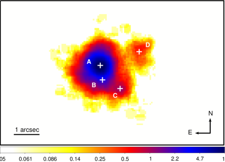
Figure 1: The X-ray image of the quadruply lensed quasar 2MASS J1042+1641 obtained with Chandra (smoothed with a 0.375^′′ boxcar). The colour bar shows the scaling of the image (in counts). Evidence for X-ray emission is seen from all four of the known images of the quasar (positions indicated by white crosses, based on Glikman et al. 2018). Image A dominates the total flux, image B is just to the south (and is blended with the emission from image A), image C is further to the south-west, and image D is the furthest to the west.

3.1.1 Image Resolved Spectroscopy

Given the visual inspection of the overall X-ray image, we initially attempt to extract separate spectra from regions associated with images A, C and D. We see no evidence for strong variability between the spectra from the two observations in any of these images individually, and so for each we combined the data from the two OBSIDs using addascaspec. For images C and D, contamination by the wings of the point-spread function (PSF) associated with image A is a potential concern. In order to assess the level of this contamination we take two approaches; we investigate the counts in a set of regions from a range of azimuthal angles to the north of image A that have the same size and separation from image A as the regions centred on images C and D, and we also use our more formal image modeling (see Section 3.1.2) to predict the expected contamination from image A in the extraction regions used for images C and D. Both approaches suggest that the expected level of contamination is $\sim$15–20% for the spectra extracted from both images C and D, which, although not completely negligible, we consider to be a reasonably manageable level. Any contamination from image B to the data from the image A should also be negligible (see Section 3.1.2).

To test whether the spectra from the individual images are consistent, we model these combined spectra with a phenomenological absorbed powerlaw model, fitting the data over the 0.5–8 keV energy range with XSPEC  v12.10.1s (Arnaud 1996). We include the Galactic absorption column ($N_{\rm{H,Gal}}=2.18\times 10^{20}$ $\rm\thinspace cm^{-2}$; HI4PI Collaboration et al. 2016), as well as a second absorber intrinsic to 2MASS J1042+1641 (i.e. at $z=2.517$); neutral absorption is modelled with tbabs (Wilms et al. 2000). We use the absorption cross-sections of Verner et al. (1996), and adopt the solar abundances of Grevesse & Sauval (1998) throughout this work for consistency with the relxill model (García et al. 2014), which is used in our later analysis.

Owing to the low S/N for images C and D (these spectra include 110 and 91 total counts, respectively), at this stage in our analysis we rebin the individual spectra to 1 count per energy bin, and fit the data by reducing the Cash statistic (Cash 1979). We found that the values for the intrinsic column, $N_{\rm{H}}$, and the photon index, $\Gamma$, are consistent within their 90% uncertainties for all three images (note that, unless stated otherwise, we quote 90% errors as standard throughout this work). We caution, however, that owing to the low S/N of the image C/D data and the contaminating flux from image A, only large spectral variations between the quasar images would be detectable, and that more subtle differences could still be present. Nevertheless, we therefore also extracted the integrated spectrum combining all of the images together, and fit this with the same model. For the integrated spectrum, we have sufficient statistics to rebin the data to a minimum S/N of 5 (note that the S/N is calculated accounting for the background and its uncertainties), and fit by minimising $\chi^{2}$. We find $N_{\rm{H}}=2.7^{+0.6}_{-0.5}\times 10^{23}$ $\rm\thinspace cm^{-2}$  and $\Gamma=1.10\pm 0.15$. The fit is statistically very good, $\chi^{2}$ = 78 for 76 degrees of freedom (DoF), but despite the fairly large absorption column the photon index is still unusually hard for a radio-quiet AGN (which typically have $\Gamma\sim 1.9$; e.g. Ricci et al. 2017a). Allowing the absorption to be partially covering (using the partcov model within XSPEC) only provides a marginal improvement in the fit ($\chi^{2}$/DoF = 73/75) and does not change the conclusion regarding the photon index significantly; the best-fit column increases slightly to $N_{\rm{H}}=(3.9\pm 1.1)\times 10^{23}$ $\rm\thinspace cm^{-2}$ and has a covering factor of $C_{\rm{f}}=95\pm 3$ %, but we still find $\Gamma=1.26\pm 0.20$.

Using the simpler model with a fully covering absorber and assuming the spectral parameters quoted above are common to all the quasar images (although we stress that the model is still a purely phenomenological description of the data at this stage), we return to the data for the individual images to determine their X-ray flux ratios. Similar to the nomenclature used in Glikman et al. (2018), we quote the image ratios relative to image C. The flux ratios we find are A/C = $13.1^{+2.4}_{-1.9}$ and D/C = $0.76^{+0.20}_{-0.16}$. These are consistent with the average flux ratios reported by Glikman et al. (2018) based on the longer wavelength HST WFC3 imaging with the F125W and F160W filters. We caution, though, that Glikman et al. (2018) find evidence that the optical/IR flux ratios may be mildly variable (by up to $\sim$50%) on timescales comparable to the separation of the X-ray observations considered here (although they also note that this could be at least in part related to modelling issues related to the diffraction spikes from image A, which intercept the other quasar images during their second HST epoch); similar variability would certainly be permitted by these results, particularly thanks to the low S/N for images C and D.

3.1.2 Image Modelling

In addition to considering these image-resolved spectra, we also perform a more direct imaging analysis of the Chandra data to determine the image flux ratios more robustly. For each observation a model of the Chandra PSF is simulated at the position of 2MASS J1042+1641 with MARX v5.5.0 using the average source spectrum assuming the fully-covering absorber described above and the observation-specific attitude file as input. We then perform two-dimensional profile fits to the Chandra images with the sherpa modelling and fitting package, using the Cash statistic and the Nelder-Mead algorithm to determine the best fit and evaluate parameter uncertainties. The image PSF is convolved with a model consisting of four Gaussians. The relative positions of these Gaussians are fixed based on the relative positions of the quasar images based on the HST astrometry (Glikman et al. 2018), but for each observation a global positional offset is allowed to account for any differences in the overall astrometric solutions between the Chandra and HST observations. A constant was added to the source model to account for the small background contribution in the Chandra image. This model is then fit to the data from the respective Chandra exposures. The fits were carried out in 80$\times$80 pixel region centred on the QSO position. The Gaussian widths are fixed between all lensed images and between both observations. The free parameters are the normalisations of the Gaussian components and the background constant, the global width of the Gaussian components, and the positional offsets. In both observations, we find that the Chandra data prefer a small astrometric shift of $\sim$0.04^′′ relative to HST.

The flux ratios are initially calculated for the two Chandra observations separately, and the results obtained are presented in Table 2. Ultimately, though, the results for the two epochs are consistent at the 90% level, and so we combine the two epochs together to determine our final constraints. The results from this analysis for the A/C and D/C ratios are consistent with those found from the spectra extracted for these images. As noted above, we also use the above model to try and predict the level of contamination from the wings of the PSF From image A in the extraction regions used for images C and D by turning the emission from image A and comparing the predicted fluxes in image C/D regions to that of the best-fit model; we find the predicted level of contamination to be $\sim$15–20%. Indeed, the consistency of the flux ratios between this imaging-based analysis (which properly considers the blending of the PSFs) and the analysis of the spectra from the different image regions above (which does not) further suggests that contamination of images C and D by the wings of the PSF of image A is not too severe, and thus should not have a major impact on the comparison of the spectra from these images discussed above.

We also note that the X-ray flux ratios from this analysis are again very similar to the average ratios reported by Glikman et al. (2018) based on the HST WFC3 imaging (although we caution again that these authors find the flux ratios may be mildly variable at optical/IR wavelengths). We therefore conclude that the same flux anomaly seen at longer wavelengths (i.e. the fact that image A is by far the brightest) is also present in the X-ray band.

Table 2: X-ray flux ratios for the four lensed images of 2MASS J1042+1641

Epoch	A/C	B/C	D/C
1	$9.6^{+3.0}_{-3.1}$	$1.6^{+0.6}_{-0.7}$	$0.4\pm 0.2$
2	$17.0^{+5.8}_{-6.2}$	$2.0\pm 1.0$	$0.7\pm 0.3$
Combined	$13.3^{+3.2}_{-3.5}$	$1.8\pm 0.6$	$0.6\pm 0.2$

3.2 Broadband Spectroscopy

Having found there are no discernible differences between the spectra extracted from the regions dominated by the different quasar images, we now turn to broadband spectroscopy, incorporating the XMM-Newton and NuSTAR data. Neither of these missions are able to resolve the separate images of the quasar, so we compare them against the integrated Chandra data from all of the images. We see no significant variability between the Chandra and XMM-Newton datasets. Similarly, we see no evidence for variability between any of the NuSTAR observations (Table 1), so we combine the data from all of these into one spectrum (again using addascaspec). As with the integrated Chandra data, we rebin the XMM-Newton and integrated NuSTAR data to have a S/N of 5 per energy bin in the same manner. We show all of these datasets (Chandra, XMM-Newton and NuSTAR) in Figure 2. 2MASS J1042+1641 is detected up to $\sim$40 keV in the NuSTAR data (corresponding to a rest-frame energy of $\sim$140 keV for 2MASS J1042+1641). Since the different datasets are all consistent with one another, in the following sections we explore models for the broadband spectrum by modelling them simultaneously. As is standard, during our analysis we allow multiplicative constants to float between them to account for cross-calibration issues, fixing the constant for the Chandra data to unity. The rest of these constants are always within $\sim$5% of unity, as expected based on detailed cross-calibration studies comparing the facilities used here (Madsen et al. 2015).

As indicated by the phenomenological fits to the Chandra data, the source spectrum is clearly very hard, as expected for an absorbed source, but also exhibits strong curvature at higher energies, peaking at $\sim$7 keV (observed frame). This corresponds to $\sim$25 keV in the quasar rest-frame, and likely indicates a significant contribution from Compton reflection (i.e. the ‘Compton hump’ that is characteristic for reprocessing by Compton-thick material, e.g. George & Fabian 1991). There is also evidence for narrow iron emission at $\sim$1.8 keV (rest-frame energy of $\sim$6.4 keV). Indeed, fitting the rest-frame 2–10 keV energy range with the absorbed powerlaw model described above, but here utilizing the full XMM-Newton and Chandra data (the relevant energies are outside of the NuSTAR bandpass), the addition of a narrow (zero-width) Gaussian emission line at 6.4 keV improves the fit by $\Delta\chi^{2}$ = 26 for one additional free parameter (the continuum parameters are consistent with those reported above for just the Chandra data). Each of the ACIS, EPIC-pn and EPIC-MOS datasets contribute roughly evenly to this improvement. We find a rest-frame equivalent width of $EW=220\pm 80$ eV (and similar continuum parameters to those quoted above). This is somewhat intermediate to the values typically seen from unobscured type-1 AGN ($EW\sim 100$ eV; e.g. Bianchi et al. 2007) and the most obscured, Compton-thick AGN ($EW\sim 1$ keV; e.g. Boorman et al. 2018). We also show in Figure 3 the results of a broader emission/absorption line search, obtained by scanning a narrow Gaussian line across the 4–10 keV bandpass in the restframe of 2MASS J1042+1641, allowing for the line to be in either emission or absorption. Aside from the strong statistical improvement provided by the Fe K emission, the available data do not show any compelling evidence for any other line features.

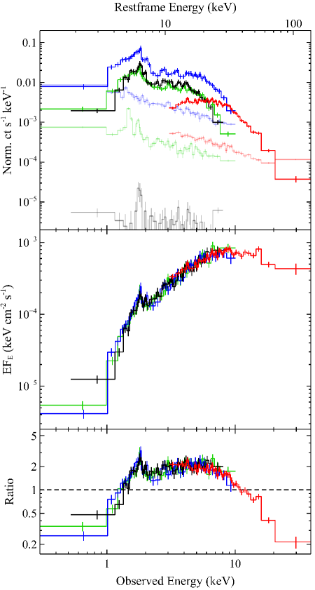
Figure 2: The broadband X-ray spectrum of 2MASS J1042+1641. The top panel shows the raw count spectra, with data from the Chandra ACIS-S detector, the NuSTAR FPMs, and the XMM-Newton EPIC-pn and EPIC-MOS detectors are shown in black, red, blue and green, respectively. The associated background levels for each detector are shown in the lighter shading for each colour. 2MASS J1042+1641 is detected up to $\sim$40 keV in the observed frame by NuSTAR, corresponding to $\sim$140 keV in the rest-frame of 2MASS J1042+1641. The middle panel shows these data unfolded through a model that is constant with energy, and the bottom panel shows the data as a ratio to a fit (to the full band) with a phenomenological powerlaw continuum, modified only by Galactic absorption ($\Gamma\sim 0.8$, $N_{\rm{H,Gal}}=2.18\times 10^{20}$ $\rm\thinspace cm^{-2}$). These panels show clear iron emission, and highlight the strong curvature in the continuum emission at higher energies (peaking at $\sim$7 keV in the observed frame). The data in all panels have been further rebinned for visual clarity.

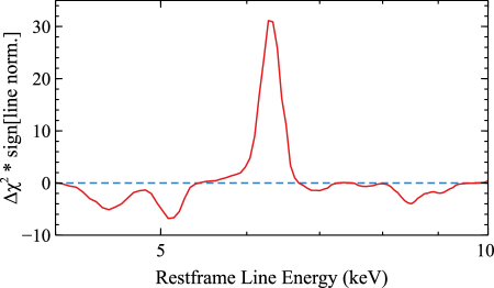
Figure 3: Results from a Gaussian line scan applied to the combined XMM-Newton and Chandra data over the 4–10 keV band, assuming a simple absorbed powerlaw continuum. The line is assumed to be unresolved and its energy is varied in increments of 60 eV, with the improvement in $\chi^{2}$ noted for each step. Positive values of $\Delta\chi^{2}$ indicate emission features, and negative values indicate absorption. The only feature of any note is the Fe K emission line at $\sim$6.4 keV.

Fitting now the full observed energy range (combining the 0.3–10 keV data from XMM-Newton, the 0.5–8 keV data from Chandra and the 3–40 keV data from NuSTAR to give a total coverage of 0.3–40 keV in the observed frame, corresponding to 1–140 keV in the rest-frame of 2MASS J1042+1641) and including an exponential high-energy cutoff in the powerlaw continuum, we find this phenomenological model provides a reasonably good description of the data, with $\chi^{2}$/DoF = 432/383. However, we still find the same issues with the continuum parameters as when considering the more limited rest-frame 2–10 keV energy range. Although the absorption column remains similar, $N_{\rm{H}}=(2.5\pm 0.4)\times 10^{23}$ $\rm\thinspace cm^{-2}$, the best-fit photon index has actually become even harder, $\Gamma=0.44\pm 0.13$. The high-energy cutoff is $E_{\rm{cut}}$ = $23^{+3}_{-2}$ keV (evaluated in the rest-frame of 2MASS J1042+1641), which is also abnormally low; AGN typically have $E_{\rm{cut}}$ $\gtrsim$ 50–100 keV (e.g. Fabian et al. 2015, Tortosa et al. 2018, Baloković et al. 2020, although there are rare exceptions, e.g. Kara et al. 2017). This again suggests that the curvature seen at high-energies is at least partially set by a significant contribution from Compton reflection. As before, these results do not change significantly if we allow the absorption to be partially covering. They also do not change significantly if we allow the absorption to be partially ionised instead (using the xstar photoionisation code; Kallman & Bautista 2001).

3.2.1 Torus Modelling

Given that the simple absorbed powerlaw models considered above for the Chandra data all imply unusually hard photon indices, and the broadband data also imply the presence of reprocessing, we now test more complex models that include both processes. We start by exploring whether the broadband data can be explained by absorption and reprocessing in an obscuring torus, as invoked in the classic unified model for AGN (e.g. Antonucci 1993). In particular, we utilize the borus model (Baloković et al. 2018), one of the most recent additions to the family of X-ray torus models (and an update of the torus model presented by Brightman & Nandra 2011). This model self-consistently computes the absorption and reprocessing assuming the obscuring medium has a uniform spherical geometry with conical polar cut-outs, is neutral, and is illuminated internally by a central continuum flux. In general, its key free parameters are the radial column density ($N_{\rm{H,tor}}$), iron abundance ($A_{\rm{Fe}}$) and opening angle of the torus ($\theta_{\rm{tor}}$), the viewing angle ($i$) and the primary continuum parameters (see below).

We initially test a model in which we are viewing the source through the torus, such that the column along our line-of-sight is the same as that of the torus (i.e. $N_{\rm{H,los}}=N_{\rm{H,tor}}$). We again use tbabs for the line-of-sight photoelectric absorption, combined with cabs to account for the scattering losses in the absorber, both of which are applied to the intrinsic AGN continuum. In addition, we also include both the reprocessed emission from borus and a fraction of the intrinsic continuum that is scattered around the absorber. These last two components are not subject to absorption by the main absorber, and are only subject to the Galactic absorption column (again fixed at $N_{\rm{H,Gal}}=2.18\times 10^{20}$ $\rm\thinspace cm^{-2}$). This is a standard borus setup for studying heavily obscured AGN (e.g. Baloković et al. 2018). In XSPEC parlance, the model expression is tbabs_Gal $\times$ $($borus $+$ CONT_scat $+$ $($tbabs_los $\times$ cabs $\times$ CONT${}_{\rm{int}}))$, where CONT indicates the AGN continuum model. To ensure we are looking through the obscurer, we first employ a version of borus that assumes the absorber covers the full $4\pi$ solid angle (i.e. has a spherical geometry). Formally, we use the borus11 model, which uses the nthcomp thermal Comptonisation model for the intrinsinc AGN continuum (parameterised by $\Gamma$ and the electron temperature, $kT_{\rm{e}}$; Zdziarski et al. 1996; Zycki et al. 1999), again evaluated in the rest-frame of 2MASS J1042+1641. Note that because the geometry is spherical here, the viewing angle is not a free parameter (the illuminating continuum is also assumed to be isotropic in borus). All of the relevant model parameters are linked between the intrinsic AGN continuum, the borus model, and the scattered AGN continuum (i.e. $\Gamma$, $kT_{\rm{e}}$, continuum normalisations). For the latter, the scattered fraction is computed via a further multiplicative constant. The iron abundances of the absorption and borus components are also linked, after scaling the borus iron abundance to that of Grevesse & Sauval (1998) for self-consistency (borus is formally calculated assuming the solar abundances of Anders & Grevesse 1989).

Table 3: Results obtained with the torus models for 2MASS J1042+1641.

Parameter	Units	Model Value
		borus11	borus12
$N_{\rm{H,los}}$	[$10^{23}$ $\rm\thinspace cm^{-2}$]	$3.0\pm 0.3$	$3.8^{+0.5}_{-0.3}$
$A_{\rm{Fe}}$	[solar]	$1.1^{+0.3}_{-0.2}$	$0.55^{+0.17}_{-0.10}$
$N_{\rm{H,tor}}$	[$10^{23}$ $\rm\thinspace cm^{-2}$]	= $N_{\rm{H,los}}$	$>31$
$\Omega_{\rm{tor}}/4\pi$		1.0[a]	$>0.61$[b]
$i$	[∘]	–	20[a]
$\Gamma$		$<1.41$[c]	$1.72^{+0.04}_{-0.12}$
$kT_{\rm{e}}$	[keV]	$11.3^{+0.5}_{-0.4}$	$26^{+7}_{-9}$
Norm	[$10^{-4}$]	$7.0^{+0.4}_{-0.3}$	$16^{+5}_{-3}$
$f_{\rm{scat}}$	[%]	$4.4\pm 1.2$	$1.6\pm 0.7$
$\chi^{2}$/DoF		381/382	359/380

This model formally fits the data very well, with $\chi^{2}$ = 381 for 382 DoF; the full results are presented in Table 3. The column density of $N_{\rm{H,tor}}\sim 3\times 10^{23}$ $\rm\thinspace cm^{-2}$ is similar to that found considering just the Chandra data, and the scattered continuum fraction is $f_{\rm{scat}}=4.4\pm 1.2$%, broadly similar to the values typically seen in local AGN (which are also at the level of a few per cent, e.g. Winter et al. 2009; Eguchi et al. 2009; Walton et al. 2018, 2019; Kammoun et al. 2020). However, the continuum parameters are still abnormal for a radio-quiet AGN. The photon index of $\Gamma<1.41$ (note that borus is only calculated for $\Gamma>1.4$) is still much harder than would be expected for such sources. Furthermore, in order to reproduce the strong high-energy curvature with such a hard continuum at lower energies, the electron temperature of $kT_{\rm{e}}$ = $11.3^{+0.5}_{-0.4}$ keV is also lower than usually seen in local AGN (as noted above, typically $E_{\rm{cut}}$ $\gtrsim$ 50–100 keV, corresponding to $kT_{\rm{e}}$ $\gtrsim$ 30 keV). This is in large part because the torus is required to be Compton-thin in this scenario, and so does not provide any notable reprocessing at high-energies. If we force the column to be Compton-thick here, i.e.  $N_{\rm{H}}>1.5\times 10^{24}$ $\rm\thinspace cm^{-2}$, the fit degrades to $\chi^{2}$/DoF = 1321/382. Although we show the results for a spherical obscurer, we stress that these conclusions do not change if we instead use a version of borus with a variable covering factor (i.e. borus12, which again uses the nthcomp model for the intrinsic continuum; Baloković et al. 2019), as long as the requirement that the column density of the torus is the same as the line-of-sight column density is retained.

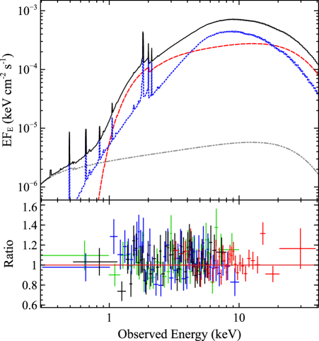
Figure 4: The torus model fit to the Chandra+NuSTAR+XMM-Newton data for 2MASS J1042+1641, using the borus12 model (see Table 3 for the best-fit parameters). The top panel shows the relative contribution of the different model components: the total model is shown in solid black, the primary powerlaw emission in dashed red, the reprocessed emission from the torus in dotted blue, and the scattered continuum in dash-dot-dot grey. The bottom panel shows the data/model ratios for the broadband dataset; here the different colours have the same meanings as in Figure 2.

We therefore test the alternative assumption, that we are not viewing the central source through the bulk of the reprocessing torus, which instead primarily lies out of our line-of-sight (i.e. $N_{\rm{H,los}}<N_{\rm{H,tor}}$), continuing with the use of the borus12 model. In order to ensure we do not view the source through the torus, we fix the viewing angle for borus at $i=20$^∘ (roughly the minimum allowed by the model), and limit its covering factor such that the reprocessing torus cannot impinge on this line-of-sight (i.e. we set a limit of $\Omega_{\rm{tor}}/4\pi<0.9$); the rest of the model setup is the same as described previously. This approach also gives a good fit to the data, with $\chi^{2}$/DoF = 359/380, and as before the full results are given in Table 3. The line-of-sight column density is similar to that inferred previously, $N_{\rm{H,los}}=3.8^{+0.5}_{-0.3}\times 10^{23}$ $\rm\thinspace cm^{-2}$, but, as expected, the column density inferred for the main torus is much larger, $N_{\rm{H,tor}}>3.1\times 10^{24}$ $\rm\thinspace cm^{-2}$. The covering factor of this torus must be fairly large, $\Omega_{\rm{tor}}/4\pi>0.61$, in order to produce the strong high-energy curvature, despite the fact that we cannot be viewing the source through an absorber with such a large column. The iron abundance in this case is mildly sub-solar, as the equivalent width of the narrow iron emission is not particularly large. However, thanks to the strong contribution from the reprocessed continuum, the continuum parameters for this model ($\Gamma$, $kT_{\rm{e}}$) are significantly closer to those expected from a radio-quiet AGN (although the electron temperature is still a little on the low side). We show this model and the corresponding data/model ratio in Figure 4.

Given that Glikman et al. (2018) report the presence of a broad absorption line (BAL) in the optical spectrum, specifically on the blue wing of the broad Mg II emission line, we again test whether the X-ray absorption could be associated with partially ionised material in an outflow now that we are considering the full broadband spectrum. Replacing the neutral absorber with a photoionised absorption model, using the same xstar as used previously, does not provide any statistical improvement over the neutral absorber, and the key parameters for the AGN emission remain essentially identical to those reported in Table 3.

Table 4: Results obtained with the relativistic disc reflection model for 2MASS J1042+1641.

Parameter	Unit	Model Value
$N_{\rm{H,los}}$	[$10^{23}$ $\rm\thinspace cm^{-2}$]	$3.2^{+0.5}_{-0.4}$
$A_{\rm{Fe}}$	[solar]	$0.9\pm 0.3$
$\Gamma$		$1.61^{+0.19}_{-0.07}$
$kT_{\rm{e}}$	[keV]	$31^{+126}_{-8}$
$h$	[$R_{\rm{G}}$]	5[a]
$a^{*}$		0.7[a]
$i$	[∘]	$<36$
$\log\xi$	$\log$[erg cm s-1]	0[a]
$R_{\rm{frac}}$		$1.7^{+2.9}_{-0.5}$
Norm	[$10^{-5}$]	$2.7^{+0.4}_{-0.8}$
$EW_{\rm{FeK}}$[b]	[eV]	$170^{+100}_{-90}$
$f_{\rm{scat}}$	[%]	$2.9^{+0.9}_{-0.8}$
$\chi^{2}$/DoF		352/379

3.2.2 Disc Reflection Modelling

We also test the scenario in which the majority of the reprocessing occurs in the accretion disc instead of a Compton-thick torus. In this case, the rapid orbital motion in the disc and the strong gravity close to the black hole broaden and skew the narrow, rest-frame emission lines into a characteristic ‘diskline’ profile (e.g. Fabian et al. 1989; Dauser et al. 2010). Evidence for reflection from the accretion disc has been seen in other, less obscured lensed quasars in the form of such relativistically broadened iron emission lines (e.g. Reis et al. 2014; Reynolds et al. 2014; Walton et al. 2015).

For this analysis we use the relxilllp_cp model (v1.3.3; García et al. 2014), which self-consistently calculates the expected reflection spectrum assuming a lamppost geometry (characterised by the height of the X-ray source above the disc, $h$) and assumes the nthcomp model for the primary X-ray continuum (which is also included in the model. The other key model parameters are the spin of the black hole, $a^{*}$, the reflection fraction, $R_{\rm{frac}}$ (which sets the relative contribution of the reflected emission; see Dauser et al. 2016 for the definition of $R_{\rm{frac}}$ used in relxilllp_cp), and the inner and outer radii, inclination, iron abundance and ionisation parameter, $\xi$, of the disc. As is standard, the ionisation parameter is defined as $\xi=L_{\rm{ion}}/nR^{2}$, where $L_{\rm{ion}}$ is the ionising luminosity (integrated between 0.1–1000 keV in the relxill models), $n$ is the density of the material, and $R$ is the distance to the ionising source.

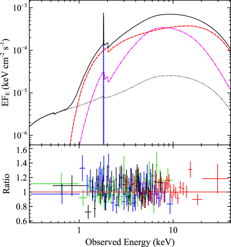
Figure 5: The disc reflection model fit to the Chandra+NuSTAR+XMM-Newton data for 2MASS J1042+1641 (see Table 4 for the best-fit parameters). As in Figure 4, the top panel shows the relative contribution of the different model components: the total model is shown in solid black, the primary nthcomp continuum in dashed red and the disc reflection in dash-dot magenta (which together form the relxilllp_cp model), the narrow Fe K line in dotted blue, and the scattered continuum in dash-dot-dot grey. The bottom panel again shows the data/model ratios, and the colours have the same meanings as in Figure 2.

As before, we include neutral absorption from our own Galaxy, and allow for neutral absorption in the rest-frame of the source, as well as some scattered fraction of the intrinsic emission that leaks around the rest-frame absorber. We also include a narrow core to the iron emission, which still likely arises from reprocessing by distant material (and so is not subject to the relativistic effects modelled by relxilllp_cp); here we treat this as a Gaussian emission line for simplicity. Overall, the model setup is similar to that outlined in Section 3.2.1, where CONT equates to the relxilllp_cp model here, and borus is replaced by the Gaussian component. During our analysis, we assume that the inner accretion disc reaches the innermost stable circular orbit (ISCO), and fix the outer disk to 1000 $R_{\rm{G}}$ (the maximum allowed by the model; $R_{\rm{G}}$ = $GM_{\rm{BH}}/c^{2}$ is the gravitational radius). As before, we also link the iron abundance between the rest-frame absorber and the relxilllp_cp components. Furthermore, the data do not have sufficient S/N to constrain the other key parameters that control the precise form of the relativistic blurring ($a^{*}$ and $h$), so we fix these to $a^{*}=0.7$ and $h=5$ $R_{\rm{G}}$, respectively; the former is the spin implied by the average radiative efficiency of $\eta=0.1$ inferred for quasars (Soltan 1982), and the latter is motivated by constraints on X-ray emitting regions from micro-lensing studies of other, less obscured lensed quasars (e.g. Dai et al. 2010; MacLeod et al. 2015). If we allow the spin to vary, we find it to be completely unconstrained by the current data. We also find the ionisation of the disc is not well constrained, so for simplicity we assume that the disk is close to being neutral (i.e. $\log[\xi/(\rm{erg}~{}\rm{cm}~{}\rm{s}^{-1})]=0$).

This model also fits the data very well, with $\chi^{2}$/DoF = 353/379; the results are presented in Table 4, and the fit is shown in Figure 5. The line-of-sight column density is similar to that found previously, $N_{\rm{H,los}}=3.2^{+0.5}_{-0.4}\times 10^{23}$ $\rm\thinspace cm^{-2}$, and the primary continuum parameters ($\Gamma$, $kT_{\rm{e}}$) are again consistent with expectation for a radio-quiet AGN. The reflection fraction of $R_{\rm{frac}}=1.7^{+2.9}_{-0.6}$ is consistent with both standard values for local, unobscured AGN ($R_{\rm{frac}}\sim 1-1.5$, e.g. Walton et al. 2013, corresponding to the rough expectation for standard illumination of a thin accretion disc, e.g. Dauser et al. 2016) or a reflection-dominated scenario ($R_{\rm{frac}}>2$). In the context of disc reflection, the latter scenario is possible if the corona is particularly compact, such that the primary X-ray continuum emission experiences strong gravitational lightbending (e.g. Miniutti & Fabian 2004), and examples of reflection-dominated states have been seen among local AGN (e.g. Parker et al. 2014; Walton et al. 2020). We also note that the best-fit iron abundance in this scenario is close to the solar value. Interestingly, the inclination of the accretion disc is inferred to be low with this model, $i<36$^∘, i.e. we would be viewing the disc close to face-on, despite the fairly heavy line-of-sight obscuration.

Finally, we note that we again tried replacing the neutral absorber in the disc reflection model with the xstar photoionisation model used previously, but as with the torus model this did not result in any statistical improvement to the fit, and all of the key parameters for the AGN emission remain the same as reported in Table 4.

4 Discussion & Conclusions

We have presented the first sensitive X-ray view of the reddened, strongly lensed quasar 2MASS J1042+1641 ($z=2.517$), combining data from the Chandra, XMM-Newton and NuSTAR observatories. This is a quadruply lensed system, based on optical/IR imaging (Glikman et al. 2018), and the Chandra data show clear X-ray emission from each of the four quasar images (see Figure 1). The flux ratios are consistent with those seen at longer wavelengths, and, within the limitations of the available data, we do not see any evidence for large differences in their X-ray spectra (which can occur if some of the intervening absorption occurs in the lensing galaxy, e.g. the cases of B1152+199 and GraL J234330.6+043557.9; Toft et al. 2000; Dai & Kochanek 2009; Krone-Martins et al. 2019). This is consistent with the absorption being intrinsic to the background quasar, as concluded by Glikman et al. (2018) and assumed throughout this work. The X-ray flux ratios show that the flux anomaly seen at longer wavelengths, in which image A dominates the total flux, is also clearly seen in the X-ray data. Glikman et al. (2018) suggest that this may be due to substructure (as predicted by $\Lambda$CDM) surrounding the main lensing galaxy (e.g. Mao & Schneider 1998), as opposed to the microlensing alternative, as they argue that the flux anomaly is still seen at longer wavelengths where microlensing should be less of an issue. The fact that the image flux ratios seem to be similar in both the X-ray and the IR bands would be consistent with this interpretation, although the reasonably large uncertainties (Table 5) mean that strong conclusions cannot be drawn from the X-ray data here. It is also worth noting, though, that the long-term X-ray lightcurve (which formally shows the integrated flux, but in reality is likely dominated by image A) appears to be relatively stable over a baseline of $\sim$8–9 years (in the observed frame; see Fig. 6); there is a hint of a variability event in the XRT data just prior to MJD 58800, but the uncertainties on the most elevated data points are extremely large.

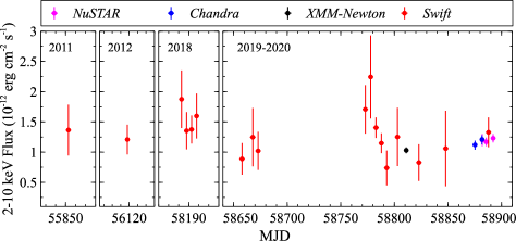
Figure 6: The long-term X-ray lightcurve of 2MASS J1042+1641 in the 2–10 keV band (observed frame). The XMM-Newton, Chandra and NuSTAR fluxes are those reported in Table 1, while the Swift data were originally generated using the online pipeline (Evans et al. 2009) with 5 d time bins, and count rates then converted to flux based on the simple absorbed powerlaw fit to the combined 2–10 keV XMM-Newton, Chandra and NuSTAR data presented in Section 3.2.

Combining all of the data, we have coverage of the $\sim$0.3–40 keV band in the observed frame, corresponding to $\sim$1–140 keV in the rest-frame of 2MASS J1042+1641. The broadband data reveal a very hard X-ray spectrum at lower energies, similar to that reported by Matsuoka et al. (2018) based on Swift data, and strong curvature of the continuum emission at higher energies (see Figure 2). This curvature peaks at a rest-frame energy of $\sim$30 keV, implying a strong contribution from reprocessing by Compton-thick material. Indeed, based on detailed modelling of the X-ray spectrum, we find that this must be the case in order to reproduce the observed data with sensible parameters for the primary AGN continuum. However, this reprocessing cannot be associated with the line-of-sight absorber, which must be Compton-thin; we find $N_{\rm{H,los}}\sim 3-4\times 10^{23}$ $\rm\thinspace cm^{-2}$, depending on the precise model used for the broader continuum, but in all cases Compton-thick solutions for the line-of-sight absorption are strongly ruled out by the data. The Compton-thin nature of the X-ray absorption is qualitatively consistent with the broad emission lines observed in the optical data (Matsuoka et al. 2018; Glikman et al. 2018). While we have been able to undertake a much more detailed spectral analysis, the line-of-sight column density found here is broadly similar to that inferred from the lower S/N Swift data (Matsuoka et al. 2018). Although this column density is large, and places 2MASS J1042+1641 as the most obscured lensed quasar observed to date, we are still lacking any lensed systems for which the line-of-sight column is Compton-thick, despite the fact that the latest estimates find that this should be the case for $\sim$30–50% of all quasars, either based on direct searches for Compton-thick sources or population synthesis modelling of the cosmic X-ray background (e.g. Lansbury et al. 2017; Lanzuisi et al. 2018; Ananna et al. 2019). However, we stress that the majority of the lensed quasars known have been identified through optical imaging (e.g. Lemon et al. 2018, 2019; Khramtsov et al. 2019; Stern et al. 2020), which is heavily biased against highly obscured systems.

The reprocessed emission observed must therefore be associated with Compton-thick material located away from our line-of-sight. We test two possible scenarios, and find the data can be equally well fit with models in which the reprocessing occurs in a torus-like structure (as invoked in the classic AGN unification model; e.g. Antonucci 1993) with $N_{\rm{H,tor}}>3.1\times 10^{24}$ $\rm\thinspace cm^{-2}$, or occurs in the accretion disc (as seen in other, unobscured lensed quasars; e.g. Reis et al. 2014; Reynolds et al. 2014; Walton et al. 2015). In the former case, the covering factor of the Compton-thick torus is inferred to be fairly large, $\Omega_{\rm{tor}}/4\pi>0.61$, even through we cannot be viewing the central source through it. This would imply a viewing angle of $i\lesssim 50$^∘, assuming the torus is an equatorial structure. In the latter case, we find a tighter constraint on the inclination, $i<36$^∘, directly from the disc reflection model. In both cases, we would therefore infer that there is still a significant column of neutral gas that obscures the central source away from equatorial lines of sight, implying that this component may have a more spherical than equatorial geometry. This may exist in addition to a thicker, more equatorial structure, or it could even be the primary structure of neutral gas surrounding the central source (if the reprocessing occurs in the inner accretion disc). In either case, the overall distribution of neutral gas around 2MASS J1042+1641 appears to differ from the simplest picture of a purely equatorial torus.

4.1 L_X vs L_IR

Following Stern (2015), we place 2MASS J1042+1641 in the context of other quasars/AGN, both in terms of its observed and intrinsic properties, by investigating where it lies in the X-ray vs IR luminosity plane (specifically, rest-frame 2–10 keV vs 6$\mu$m). Here, we quote fluxes integrated over all four of the quasar images, mimicking the results that would be seen with X-ray and IR surveys that do not have the imaging resolution to separate them. The total observed flux in the rest-frame 2–10 keV band is $F_{2-10,\rm{obs}}=1.8\pm 0.7\times 10^{-13}$ $\rm\thinspace erg~{}cm^{-2}~{}s^{-1}$, corresponding to a luminosity of $L_{2-10,\rm{obs}}=9\pm 3\times 10^{45}$ erg s^-1 for a luminosity distance of $D_{\rm{L}}=2\times 10^{4}$ Mpc. Correcting the X-ray flux for the line-of-sight absorption, we find $L_{2-10,\rm{unabs}}=(2.7\pm 0.7)\times 10^{46}$ erg s^-1 (as the two preferred models considered here both have similar column densities, there is good agreement between them regarding the absorption correction, and the uncertainty range given here represents their combined uncertainty range). Finally, we de-magnify the flux to compute the intrinsic 2–10 keV luminosity, $L_{\rm{2-10,int}}$. At the time of writing, Glikman et al. (2018) present two estimates for the total magnification: $\mu_{\rm{mag}}=53\pm 5$, based purely on their current lens modelling, and $\mu_{\rm{mag}}=122\pm 26$, based on a combination of their lens modelling and the image flux ratios observed in the IR by HST. An independent lens modelling by Schmidt et al. (submitted) that combines these IR data with more recent UV data from HST also finds a magnification factor of $\mu_{\rm{mag}}\sim 51$, in good agreement with the equivalent analysis in Glikman et al. (2018). Nevertheless, give the contrasting values reported by Glikman et al. (2018), to be conservative we present estimates for $L_{\rm{2-10,int}}$ (and various quantities derived subsequently) for both magnification factors (see Table 5). We find $L_{2-10,\rm{int}}\sim$ $2-5\times 10^{44}$ erg s^-1. Similarly, the total observed luminosity at $6\mu$m is $L_{\rm 6,obs}=4.6\times 10^{47}$ erg s^-1 based on interpolating the WISE photometry, and the intrinsic luminosity after correcting for the magnification is $L_{6,\rm{int}}\sim$ $4-9\times 10^{45}$ erg s^-1.

Table 5: Derived X-ray/IR luminosities and related quantities for 2MASS J1042+1641, given for both of the potential magnification factors reported by Glikman et al. (2018).

Quantity	Unit	$\mu_{\rm{mag}}=53$	$\mu_{\rm{mag}}=122$
$L_{\rm{2-10,int}}$	[$10^{44}$ erg s-1]	$5.1\pm 1.4$	$2.2\pm 0.7$
$L_{\rm{6,int}}$	[$10^{45}$ erg s-1]	$8.7\pm 0.8$	$3.8\pm 0.8$
$L_{\rm{15,int}}$	[$10^{45}$ erg s-1]	$11.0\pm 1.0$	$4.8\pm 1.0$
$L_{\rm{bol,int}}$[a]	[$10^{46}$ erg s-1]	$9.4\pm 1.4$	$4.1\pm 1.0$
$M_{\rm{BH}}$[b]	[$10^{9}$ $M_{\odot}$]	$8^{+2}_{-3}$	$5^{+1}_{-2}$
$\lambda_{\rm{E}}$		$0.09^{+0.04}_{-0.03}$	$0.06^{+0.03}_{-0.02}$
$\Omega_{\rm{tor,pred}}$[c]	[$4\pi$]	0.0 ($<$0.25)	0.15 ($<$0.35)

^a Assuming a bolometric correction of $8.5\pm 1.0$ for $L_{\rm{15,int}}$ from Runnoe et al. (2012).
^b From Matsuoka et al. (2018), based on H$\alpha$ and H$\beta$ line widths; quoted values are the averages of the individual H$\alpha$ and H$\beta$ estimates, and their uncertainties correspond to the full ranges given in Matsuoka et al. (2018), incorporating both H$\alpha$ and H$\beta$, and their quoted statistical uncertainties.
^c Based on Brightman et al. (2015) and $L_{\rm{2-10,int}}$; the full uncertainty range is consistent with zero in both cases, so we quote both the predicted value and its upper limit (with the latter in parentheses).

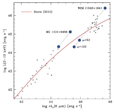
Figure 7: Rest-frame, absorption corrected 2–10 keV X-ray luminosity against rest-frame 6$\mu$m luminosity for the sample of non-lensed AGN compiled by Stern (2015). These cover a wide range luminosity; local Seyfert galaxies from Horst et al. (2008) and Gandhi et al. (2009) are shown with $\times$ symbols, while luminous quasars from Just et al. (2007) are shown with $+$ symbols. The best-fit relation between the X-ray and IR luminosities derived by Stern (2015), which is linear at lower luminosities and begins to flatten at higher luminosities, is shown with the solid red curve. Large circles show the results for 2MASS J1042+1641 both before and after the lensing magnification is accounted for. Intrinsically, 2MASS J1042+1641 lies close to observed relation, at a luminosity where the trend is roughly linear. However, the lensed values would appear to place this source far above the relation. This is similar to the lensed radio galaxy MG 1131+0456 (also shown; Stern & Walton 2020), and may suggest a new method to identify lensed AGN candidates from wide-field X-ray and IR surveys.

These values are shown in Figure 7, along with a sample of non-lensed AGN from which Stern (2015) compute their best fit relation between the 2–10 keV and 6 $\mu$m luminosities (note that these X-ray luminosities are also all corrected for line-of-sight absorption). While this is roughly linear at lower luminosities, Stern (2015) find that the trend begins to flatten at higher luminosities, such that an equivalent increase in IR luminosity would gradually correspond to a smaller and smaller increase in X-ray luminosity. Analysing the Einstein ring MG 1131+0456, Stern & Walton (2020) speculate that this might provide an opportunity to identify new lensed quasar candidates by combining wide-field X-ray and infrared surveys (e.g. eROSITA and WISE; Merloni et al. 2012; Wright et al. 2010), as sources that intrinsically lie on the linear part of the relation, when significantly magnified, would appear to have anomalously high X-ray luminosities (see also Connor et al. 2022). The results found here for 2MASS J1042+1641 would also suggest this could be a promising method; given its IR luminosity, 2MASS J1042+1641 would indeed appear to have an unusually high X-ray luminosity, but after accounting for the magnification, lies much closer to the relation for unlensed AGN. It should be stressed that this would also require significant efforts to obtain source redshifts, which would be a critical part of such an identification method. Nevertheless, this approach might be particularly appealing, as it should be most sensitive to the rare quadruply lensed systems, which have the strongest total magnification.

We note that these comparisons have assumed that the lensing magnifications are the same in the IR and X-ray bands. The fact that this does bring 2MASS J1042+1641 into better agreement with the results seen from unlensed quasars suggests that this assumption is not unreasonable. This assumption is also made in the other pilot studies of lensed quasars that have explored the idea of pre-selecting such sources based on their X-ray vs IR properties (Stern & Walton 2020; Connor et al. 2022). Indeed, if we take the lens model for 2MASS J1042+1641 presented by Glikman et al. (2018), we find that any differential magnification should be at less than the 10% level for emitting regions smaller than 10 pc. This lens model corresponds to the magnification factor of $\mu=53$, and assuming that the characteristic size scale of the torus is set by the dust sublimation radius, $R_{\rm{sub}}$, based on the expression outlined in Barvainis (1987) we find $R_{\rm{sub}}\sim 4$ pc for this magnification factor (assuming a typical grain size of 0.05 $\mu$m and a sublimation temperature of 1500 K and conservatively taking $L_{\rm{UV}}\sim L_{\rm{bol}}$). As such, assuming a common magnification factor for the X-ray and the IR data is likely a reasonable approach here. It is also worth noting that the ratio of the luminosity of the narrow iron K$\alpha$ emission – assumed to be associated with distant reprocessing – to the absorption-corrected 10–50 keV luminosity is $L_{\rm{FeK}}/L_{10-50}=3.2^{+1.1}_{-1.8}\times 10^{-3}$, assuming the two experience the same magnification; although the uncertainties are relatively large, this is extremely similar to the typical ratio seen for unlensed quasars ($\sim$3–4 $\times$ 10^-3; Ricci et al. 2014).

In general, though, it may be plausible that the X-ray and IR magnification factors are not the same if there is significant microlensing from structure in the lens, given that at least in the case of unobscured quasars the X-ray emission is expected to come from much smaller scales than the IR emission. Should this occur, the general expectation is that the more compact X-ray source would experience a larger total magnification (e.g. Chartas et al. 2012; Hutsemékers & Sluse 2021). As long as the sources are intrinsically close to the X-ray vs IR trend reported in Stern (2015), though, then enhanced X-ray magnification (vs the IR) would actually drive sources even further away from this trend and make them appear as even more extreme outliers. This method of selecting lensed quasar candidates would therefore still be suitable even in this scenario.

4.2 Reprocessing and Black Hole Growth

In principle, we may also be able to use the intrinsic 2–10 keV luminosity to estimate the expected covering factor for the Compton-thick phase of the surrounding medium, assuming that the anti-correlation between these quantities seen in local AGN (Brightman et al. 2015) also holds for 2MASS J1042+1641. For the above luminosity, we find a predicted covering factor of $\Omega_{\rm{tor,pred}}/4\pi<$ 0.35 (Table 5). If this trend does hold, we would therefore expect only a small contribution from any Compton-thick torus in terms of reprocessed emission. This would in turn suggest that, of the two scenarios considered for the dominant source of the reprocessed emission (torus vs disc reflection), the disc reflection interpretation may be the more likely solution. We stress, though, that it is not clear whether the Brightman et al. (2015) relation is still relevant here, as there is good evidence that the fraction of ‘obscured’ AGN (those with $N_{\rm{H}}>10^{22}$ $\rm\thinspace cm^{-2}$) increases with increasing redshift for a given X-ray luminosity (e.g. Ueda et al. 2014; Buchner et al. 2015). The relevant issue here, though, is whether a similar trend is also present for Compton thick AGN specifically. There is conflicting evidence over this point (Brightman & Ueda 2012 do find evidence for a qualitatively similar trend for Compton-thick AGN, while Buchner et al. 2015 find the fraction of Compton-thick AGN to be constant with redshift), but if a similar trend is present then the Brightman et al. (2015) trend would not formally be suitable for use with 2MASS J1042+1641. We also note again the contrasting magnification factors reported for this source.

Nevertheless, the nominal difference between the inferred covering factor for the Compton-thick phase of the torus and the best-fit prediction for even the lower intrinsic luminosity estimate (i.e. the one associated with $\mu_{\rm{mag}}=122$) based on Brightman et al. (2015) is pretty large. If the disc reflection model is the more appropriate solution, future efforts to obtain tighter constraints on the strength of the reflection may be of significant interest. Although the level of obscuration will make direct constraints from broad Fe K emission difficult, the strength of the reflection can still potentially provide information on the spin of the black hole if a reflection-dominated scenario can be confirmed (e.g. Dauser et al. 2014). If the potential variability event noted earlier is real, and intrinsic to the source (as opposed to driven by microlensing), then based on the masses reported in Matsuoka et al. (2018) and the observed-frame duration of $\sim$15 days light-crossing arguments would suggest the majority of the X-ray flux comes from a region of less than $\sim$10–15 $R_{\rm{G}}$ in size (broadly similar to the X-ray source sizes inferred in other lensed quasars where microlensing constraints can be placed, e.g. Dai et al. 2010; MacLeod et al. 2015). This may imply a mild preference for the disc reflection scenario, but given the large uncertainties regarding the significance of this event, also highlighted above, we strongly caution against over-interpretation here. Given the observed flux, improved constraints on the reflection may be challenging with NuSTAR, requiring extremely deep exposures, but 2MASS J1042+1641 would likely be an excellent target for the next generation of hard X-ray observatory (e.g. HEX-P; Madsen et al. 2018).

In order to estimate the intrinsic bolometric luminosity of 2MASS J1042+1641, we also extract the 15$\mu$m luminosity following the same methodology as for the 6$\mu$m luminosity, and combine this with the 15$\mu$m bolometric correction reported by Runnoe et al. (2012): $\kappa_{15}=8.5\pm 1.0$ (such that $L_{\rm{bol,int}}=\kappa_{15}L_{\rm{15,int}}$; see also Richards et al. 2006). After accounting for the two possible magnification factors considered here, we find that $L_{\rm{15,int}}$ = $5-11\times 10^{45}$ erg s^-1, implying $L_{\rm{bol,int}}$ = $4-10\times 10^{46}$ erg s^-1. These values are in excellent agreement with the bolometric luminosities reported by Matsuoka et al. (2018) based on the 5100 Å luminosity. For the masses also reported in Matsuoka et al. (2018), based on the H$\alpha$ and H$\beta$ line widths ($M_{\rm{BH}}\sim 5-8\times 10^{9}$ $M_{\odot}$), these bolometric luminosities would correspond to fairly modest Eddington ratios of $\lambda_{\rm{E}}=L_{\rm{bol,int}}/L_{\rm{E}}\sim 0.05-0.1$. Given the intrinsic X-ray luminosities calculated earlier, these bolometric luminosities would also imply a large 2-10 keV bolometric correction of $\kappa_{2-10}\sim 200$ is appropriate for 2MASS J1042+1641. In the local universe, a bolometric correction of $\kappa_{2-10}\sim 200$ would be unusually high for such modest Eddington ratios (Vasudevan & Fabian 2009; Lusso et al. 2010). However, such a correction would be broadly consistent with the connection between $\kappa_{2-10}$ and $L_{\rm{bol}}$ reported by Marconi et al. (2004), which would predict $\kappa_{2-10}\sim 100$.

Regardless, for the Eddington ratio of $\lambda_{\rm{E}}$ $\sim 0.05-0.1$ inferred here, the current luminosity of 2MASS J1042+1641 would probably not be sufficient to drive away the neutral gas and dust along our line-of-sight and bring about a classic unobscured quasar phase, assuming a standard gas-to-dust ratio. In terms of the $\lambda_{\rm{E}}$–$N_{\rm H}$ plane discussed frequently in the literature (e.g. Fabian et al. 2008; Ishibashi & Fabian 2015; Ricci et al. 2017b), 2MASS J1042+1641 currently resides in the long-lived absorption regime, computed by considering the expected radiation pressure on the accompanying dust. This is in contrast to other populations of red, obscured quasars (e.g. Banerji et al. 2014; Lansbury et al. 2020), and may have interesting implications if Matsuoka et al. (2018) are correct about the high $M_{\rm{BH}}/M_{\rm{gal}}$ ratio compared to other similar systems. Presumably this would imply that the black hole has already undergone a significant (and perhaps abnormal) amount of growth, and yet it remains buried behind a significant column of gas and dust. Either this growth was somehow unable to blow out the obscuring medium, in contrast to general expectations for quasar evolution (e.g. Hopkins et al. 2008), or this has somehow been replenished after the last major quasar phase in 2MASS J1042+1641.

Data Availability

All of the raw observational data utilized in this article are publicly available from ESA’s XMM-Newton Science Archive, NASA’s HEASARC archive, and NASA’s Chandra Data Archive.

References

- Alexander et al. (2008) Alexander D. M., Brandt W. N., Smail I., et al., 2008, AJ, 135, 5, 1968
- Ananna et al. (2019) Ananna T. T., Treister E., Urry C. M., et al., 2019, ApJ, 871, 2, 240
- Anders & Grevesse (1989) Anders E., Grevesse N., 1989, Geochimica Cosmochimica Acta, 53, 197
- Antonucci (1993) Antonucci R., 1993, ARA&A, 31, 473
- Arnaud (1996) Arnaud K. A., 1996, in Astronomical Data Analysis Software and Systems V, edited by G. H. Jacoby & J. Barnes, vol. 101 of Astron. Soc. Pac. Conference Series, Astron. Soc. Pac., San Francisco, 17
- Bade et al. (1997) Bade N., Siebert J., Lopez S., Voges W., Reimers D., 1997, A&A, 317, L13
- Baloković et al. (2018) Baloković M., Brightman M., Harrison F. A., et al., 2018, ApJ, 854, 42
- Baloković et al. (2019) Baloković M., García J. A., Cabral S. E., 2019, Research Notes of the American Astronomical Society, 3, 11, 173
- Baloković et al. (2020) Baloković M., Harrison F. A., Madejski G., et al., 2020, ApJ, 905, 1, 41
- Banerji et al. (2014) Banerji M., Fabian A. C., McMahon R. G., 2014, MNRAS, 439, L51
- Barvainis (1987) Barvainis R., 1987, ApJ, 320, 537
- Bate et al. (2011) Bate N. F., Floyd D. J. E., Webster R. L., Wyithe J. S. B., 2011, ApJ, 731, 1, 71
- Bianchi et al. (2007) Bianchi S., Guainazzi M., Matt G., Fonseca Bonilla N., 2007, A&A, 467, 1, L19
- Boorman et al. (2018) Boorman P. G., Gandhi P., Baloković M., et al., 2018, MNRAS, 477, 3, 3775
- Brandt & Alexander (2015) Brandt W. N., Alexander D. M., 2015, A&ARv, 23, 1
- Brightman et al. (2015) Brightman M., Baloković M., Stern D., et al., 2015, ApJ, 805, 41
- Brightman & Nandra (2011) Brightman M., Nandra K., 2011, MNRAS, 413, 1206
- Brightman & Ueda (2012) Brightman M., Ueda Y., 2012, MNRAS, 423, 1, 702
- Buchner et al. (2015) Buchner J., Georgakakis A., Nandra K., et al., 2015, ApJ, 802, 2, 89
- Cash (1979) Cash W., 1979, ApJ, 228, 939
- Chartas et al. (2003) Chartas G., Brandt W. N., Gallagher S. C., 2003, ApJ, 595, 85
- Chartas et al. (2002) Chartas G., Gupta V., Garmire G., et al., 2002, ApJ, 565, 96
- Chartas et al. (2012) Chartas G., Kochanek C. S., Dai X., Moore D., Mosquera A. M., Blackburne J. A., 2012, ApJ, 757, 137
- Connor et al. (2022) Connor T., Stern D., Krone-Martins A., et al., 2022, ApJ, 927, 1, 45
- Dai & Kochanek (2009) Dai X., Kochanek C. S., 2009, ApJ, 692, 1, 677
- Dai et al. (2010) Dai X., Kochanek C. S., Chartas G., et al., 2010, ApJ, 709, 278
- Dauser et al. (2014) Dauser T., García J., Parker M. L., Fabian A. C., Wilms J., 2014, MNRAS, 444, L100
- Dauser et al. (2016) Dauser T., García J., Walton D. J., et al., 2016, A&A, 590, A76
- Dauser et al. (2010) Dauser T., Wilms J., Reynolds C. S., Brenneman L. W., 2010, MNRAS, 409, 1534
- Eguchi et al. (2009) Eguchi S., Ueda Y., Terashima Y., Mushotzky R., Tueller J., 2009, ApJ, 696, 2, 1657
- Evans et al. (2009) Evans P. A., Beardmore A. P., Page K. L., et al., 2009, MNRAS, 397, 1177
- Fabian et al. (2015) Fabian A. C., Lohfink A., Kara E., Parker M. L., Vasudevan R., Reynolds C. S., 2015, MNRAS, 451, 4375
- Fabian et al. (1989) Fabian A. C., Rees M. J., Stella L., White N. E., 1989, MNRAS, 238, 729
- Fabian et al. (2008) Fabian A. C., Vasudevan R. V., Gandhi P., 2008, MNRAS, 385, 1, L43
- Fruscione et al. (2006) Fruscione A., McDowell J. C., Allen G. E., et al., 2006, CIAO: Chandra’s data analysis system, vol. 6270 of Society of Photo-Optical Instrumentation Engineers (SPIE) Conference Series, 62701V
- Gandhi et al. (2009) Gandhi P., Horst H., Smette A., et al., 2009, A&A, 502, 2, 457
- García et al. (2014) García J., Dauser T., Lohfink A., et al., 2014, ApJ, 782, 76
- Garmire et al. (2003) Garmire G. P., Bautz M. W., Ford P. G., Nousek J. A., Ricker Jr. G. R., 2003, in SPIE Conference Series, edited by J. E. Truemper, H. D. Tananbaum, vol. 4851 of SPIE Conference Series, 28–44
- Gehrels et al. (2004) Gehrels N., Chincarini G., Giommi P., et al., 2004, ApJ, 611, 1005
- George & Fabian (1991) George I. M., Fabian A. C., 1991, MNRAS, 249, 352
- Glikman et al. (2018) Glikman E., Rusu C. E., Djorgovski S. G., et al., 2018, arXiv e-prints, arXiv:1807.05434
- Grevesse & Sauval (1998) Grevesse N., Sauval A. J., 1998, Space Sci. Rev., 85, 161
- Guainazzi et al. (2016) Guainazzi M., Risaliti G., Awaki H., et al., 2016, MNRAS, 460, 2, 1954
- Harrison et al. (2013) Harrison F. A., Craig W. W., Christensen F. E., et al., 2013, ApJ, 770, 103
- Hewitt et al. (1992) Hewitt J. N., Turner E. L., Lawrence C. R., Schneider D. P., Brody J. P., 1992, AJ, 104, 968
- HI4PI Collaboration et al. (2016) HI4PI Collaboration, Ben Bekhti N., Flöer L., et al., 2016, A&A, 594, A116
- Hopkins et al. (2008) Hopkins P. F., Hernquist L., Cox T. J., Kereš D., 2008, ApJS, 175, 2, 356
- Horst et al. (2008) Horst H., Gandhi P., Smette A., Duschl W. J., 2008, A&A, 479, 2, 389
- Hutsemékers & Sluse (2021) Hutsemékers D., Sluse D., 2021, A&A, 654, A155
- Ishibashi & Fabian (2015) Ishibashi W., Fabian A. C., 2015, MNRAS, 451, 1, 93
- Jansen et al. (2001) Jansen F., Lumb D., Altieri B., et al., 2001, A&A, 365, L1
- Just et al. (2007) Just D. W., Brandt W. N., Shemmer O., et al., 2007, ApJ, 665, 2, 1004
- Kallman & Bautista (2001) Kallman T., Bautista M., 2001, ApJS, 133, 221
- Kammoun et al. (2020) Kammoun E. S., Miller J. M., Koss M., et al., 2020, ApJ, 901, 2, 161
- Kara et al. (2017) Kara E., García J. A., Lohfink A., et al., 2017, MNRAS, 468, 3489
- Keeton et al. (2003) Keeton C. R., Gaudi B. S., Petters A. O., 2003, ApJ, 598, 1, 138
- Khramtsov et al. (2019) Khramtsov V., Sergeyev A., Spiniello C., et al., 2019, A&A, 632, A56
- Krone-Martins et al. (2019) Krone-Martins A., Graham M. J., Stern D., et al., 2019, arXiv e-prints, arXiv:1912.08977
- Lansbury et al. (2017) Lansbury G. B., Alexander D. M., Aird J., et al., 2017, ApJ, 846, 1, 20
- Lansbury et al. (2020) Lansbury G. B., Banerji M., Fabian A. C., Temple M. J., 2020, MNRAS
- Lanzuisi et al. (2018) Lanzuisi G., Civano F., Marchesi S., et al., 2018, MNRAS, 480, 2, 2578
- Lanzuisi et al. (2019) Lanzuisi G., Gilli R., Cappi M., et al., 2019, ApJ, 875, 2, L20
- Lawrence et al. (1984) Lawrence C. R., Schneider D. P., Schmidt M., et al., 1984, Science, 223, 4631, 46
- Lemon et al. (2019) Lemon C. A., Auger M. W., McMahon R. G., 2019, MNRAS, 483, 3, 4242
- Lemon et al. (2018) Lemon C. A., Auger M. W., McMahon R. G., Ostrovski F., 2018, MNRAS, 479, 4, 5060
- Li et al. (2004) Li J., Kastner J. H., Prigozhin G. Y., Schulz N. S., Feigelson E. D., Getman K. V., 2004, ApJ, 610, 2, 1204
- Lusso et al. (2010) Lusso E., Comastri A., Vignali C., et al., 2010, A&A, 512, A34
- MacLeod et al. (2015) MacLeod C. L., Morgan C. W., Mosquera A., et al., 2015, ApJ, 806, 2, 258
- Madsen et al. (2020) Madsen K. K., Grefenstette B. W., Pike S., et al., 2020, arXiv e-prints, arXiv:2005.00569
- Madsen et al. (2018) Madsen K. K., Harrison F., Broadway D., et al., 2018, vol. 10699 of Proc. SPIE, 106996M
- Madsen et al. (2015) Madsen K. K., Harrison F. A., Markwardt C. B., et al., 2015, ApJS, 220, 8
- Mao & Schneider (1998) Mao S., Schneider P., 1998, MNRAS, 295, 3, 587
- Marconi et al. (2004) Marconi A., Risaliti G., Gilli R., Hunt L. K., Maiolino R., Salvati M., 2004, MNRAS, 351, 1, 169
- Markowitz et al. (2014) Markowitz A. G., Krumpe M., Nikutta R., 2014, MNRAS, 439, 1403
- Matsuoka et al. (2018) Matsuoka K., Toba Y., Shidatsu M., et al., 2018, A&A, 620, L3
- Merloni et al. (2012) Merloni A., Predehl P., Becker W., et al., 2012, arXiv e-prints, arXiv:1209.3114
- Miniutti & Fabian (2004) Miniutti G., Fabian A. C., 2004, MNRAS, 349, 1435
- Parker et al. (2014) Parker M. L., Wilkins D. R., Fabian A. C., et al., 2014, MNRAS, 443, 1723
- Petrucci et al. (2001) Petrucci P. O., Merloni A., Fabian A., Haardt F., Gallo E., 2001, MNRAS, 328, 501
- Piconcelli et al. (2004) Piconcelli E., Jimenez-Bailón E., Guainazzi M., Schartel N., Rodríguez-Pascual P. M., Santos-Lleó M., 2004, MNRAS, 351, 161
- Reis et al. (2014) Reis R. C., Reynolds M. T., Miller J. M., Walton D. J., 2014, Nat, 507, 207
- Reynolds et al. (2014) Reynolds M. T., Walton D. J., Miller J. M., Reis R. C., 2014, ApJ, 792, L19
- Ricci et al. (2017a) Ricci C., Trakhtenbrot B., Koss M. J., et al., 2017a, ApJS, 233, 2, 17
- Ricci et al. (2017b) Ricci C., Trakhtenbrot B., Koss M. J., et al., 2017b, Nat, 549, 7673, 488
- Ricci et al. (2014) Ricci C., Ueda Y., Paltani S., Ichikawa K., Gandhi P., Awaki H., 2014, MNRAS, 441, 4, 3622
- Richards et al. (2006) Richards G. T., Lacy M., Storrie-Lombardi L. J., et al., 2006, ApJS, 166, 2, 470
- Risaliti et al. (2002) Risaliti G., Elvis M., Nicastro F., 2002, ApJ, 571, 234
- Runnoe et al. (2012) Runnoe J. C., Brotherton M. S., Shang Z., 2012, MNRAS, 426, 4, 2677
- Saha & Williams (2003) Saha P., Williams L. L. R., 2003, AJ, 125, 6, 2769
- Sluse et al. (2003) Sluse D., Surdej J., Claeskens J. F., et al., 2003, A&A, 406, L43
- Soltan (1982) Soltan A., 1982, MNRAS, 200, 115
- Stern (2015) Stern D., 2015, ApJ, 807, 2, 129
- Stern et al. (2020) Stern D., Djorgovski S. G., Krone-Martins A., et al., 2020, arXiv e-prints, arXiv:2012.10051
- Stern et al. (2010) Stern D., Jimenez R., Verde L., Stanford S. A., Kamionkowski M., 2010, ApJS, 188, 1, 280
- Stern & Walton (2020) Stern D., Walton D. J., 2020, ApJ, 895, 2, L38
- Strüder et al. (2001) Strüder L., Briel U., Dennerl K., et al., 2001, A&A, 365, L18
- Suyu et al. (2017) Suyu S. H., Bonvin V., Courbin F., et al., 2017, MNRAS, 468, 3, 2590
- Tanimoto et al. (2019) Tanimoto A., Ueda Y., Odaka H., Kawaguchi T., Fukazawa Y., Kawamuro T., 2019, ApJ, 877, 2, 95
- Toft et al. (2000) Toft S., Hjorth J., Burud I., 2000, A&A, 357, 115
- Tortosa et al. (2018) Tortosa A., Bianchi S., Marinucci A., Matt G., Petrucci P. O., 2018, A&A, 614, A37
- Turner et al. (2001) Turner M. J. L., Abbey A., Arnaud M., et al., 2001, A&A, 365, L27
- Ueda et al. (2014) Ueda Y., Akiyama M., Hasinger G., Miyaji T., Watson M. G., 2014, ApJ, 786, 2, 104
- Vasudevan & Fabian (2009) Vasudevan R. V., Fabian A. C., 2009, MNRAS, 392, 1124
- Verner et al. (1996) Verner D. A., Ferland G. J., Korista K. T., Yakovlev D. G., 1996, ApJ, 465, 487
- Walton et al. (2020) Walton D. J., Alston W. N., Kosec P., et al., 2020, MNRAS, 499, 1, 1480
- Walton et al. (2018) Walton D. J., Brightman M., Risaliti G., et al., 2018, MNRAS, 473, 4377
- Walton et al. (2013) Walton D. J., Nardini E., Fabian A. C., Gallo L. C., Reis R. C., 2013, MNRAS, 428, 2901
- Walton et al. (2019) Walton D. J., Nardini E., Gallo L. C., et al., 2019, MNRAS, 484, 2544
- Walton et al. (2015) Walton D. J., Reynolds M. T., Miller J. M., Reis R. C., Stern D., Harrison F. A., 2015, ApJ, 805, 161
- Walton et al. (2016) Walton D. J., Tomsick J. A., Madsen K. K., et al., 2016, ApJ, 826, 87
- Weisskopf et al. (2002) Weisskopf M. C., Brinkman B., Canizares C., Garmire G., Murray S., Van Speybroeck L. P., 2002, PASP, 114, 1
- Wilms et al. (2000) Wilms J., Allen A., McCray R., 2000, ApJ, 542, 914
- Winter et al. (2009) Winter L. M., Mushotzky R. F., Reynolds C. S., Tueller J., 2009, ApJ, 690, 1322
- Wright et al. (2010) Wright E. L., Eisenhardt P. R. M., Mainzer A. K., et al., 2010, AJ, 140, 1868
- Wu et al. (2018) Wu J., Jun H. D., Assef R. J., et al., 2018, ApJ, 852, 2, 96
- Zdziarski et al. (1996) Zdziarski A. A., Johnson W. N., Magdziarz P., 1996, MNRAS, 283, 193
- Zycki et al. (1999) Zycki P. T., Done C., Smith D. A., 1999, MNRAS, 309, 561