First Sample of H$\alpha$$+$[O III] $\lambda$5007 Line Emitters at $\mathbf{z>6}$ Through JWST/NIRCam Slitless Spectroscopy: Physical Properties and Line Luminosity Functions

Abstract

We present a sample of four emission-line galaxies at $z=6.11-6.35$ that were serendipitously discovered using the commissioning data for the JWST/NIRCam wide-field slitless spectroscopy (WFSS) mode. One of them (at $z$ $=$ 6.11) has been reported previously, while the others are new discoveries. These sources are selected by the secure detections of both [O III] $\lambda$5007 and H$\alpha$ lines with other fainter lines tentatively detected in some cases (e.g., [O II] $\lambda$3727, [O III] $\lambda$4959). In the [O III]/H$\beta$–[N II]/H$\alpha$ Baldwin-Phillips-Terlevich diagram, these galaxies occupy the same parameter space as that of $z\sim 2$ star-forming galaxies, indicating that they have been enriched rapidly to subsolar metallicities ($\sim 0.4\,\mathrm{Z}_{\odot}$), similar to galaxies with comparable stellar masses at much lower redshifts. The detection of strong H$\alpha$ lines suggests a higher ionizing photon production efficiency within galaxies in the early Universe. We find brightening of the [O III] $\lambda$5007 line luminosity function (LF) from $z=3$ to 6, and weak or no redshift evolution of the H$\alpha$ line LF from $z=2$ to 6. Both LFs are under-predicted at $z\sim 6$ by a factor of $\sim$10 in certain cosmological simulations. This further indicates a global Ly$\alpha$ photon escape fraction of 7–10% at $z\sim 6$, slightly lower than previous estimates through the comparison of the UV-derived star-formation rate density and Ly$\alpha$ luminosity density. Our sample recovers $66_{-44}^{+128}$% of $z=6.0-6.6$ galaxies in the survey volume with stellar masses greater than $5\times 10^{8}\,$$\mathrm{M}_{\odot}$, suggesting the ubiquity of strong H$\alpha$ and [O III] line emitters in the Epoch of Reionization, which will be further uncovered in the era of JWST.

tablenum SIXtablenum

1 Introduction

With eighteen images of the same star from each segment of the primary mirror finally aligned together, the long-awaited James Webb Space Telescope (JWST; Gardner et al. 2023) immediately started to unfold the secrets from the distant Universe. Thanks to its unprecedented sensitivity and spectroscopic capability in the near/mid-infrared (NIR/MIR) wavelengths, for the first time the rest-frame optical nebular emission lines (e.g., [O II] $\lambda\lambda$3726, 3729, H$\beta$, [O III] $\lambda\lambda$4959, 5007 and H$\alpha$) of normal star-forming galaxies can be directly detected and resolved in the Epoch of Reionization (EoR: $z$ $\gtrsim$ 6; see a recent review by Robertson 2022). The JWST/NIRSpec Early Release Observations (EROs) of the SMACS0723 lensing-cluster field (Pontoppidan et al., 2022) have immediately produced high-quality spectra for a handful of $z\sim 8$ galaxies with low stellar masses ($M_{\mathrm{star}}\lesssim 10^{8}$ $\mathrm{M}_{\odot}$). This allows numerous studies, including direct gas-phase metallicity measurements (see Arellano-Córdova et al. 2022, Brinchmann 2022, Carnall et al. 2023, Curti et al. 2023, Katz et al. 2023, Rhoads et al. 2023, Schaerer et al. 2022, Tacchella et al. 2022, Taylor et al. 2022, Trump et al. 2023). These ERO results have clearly demonstrated the power of JWST’s spectroscopic observations, initially with NIRSpec, promising many exciting discoveries to be made over the coming years.

In addition to NIRSpec, NIRCam’s wide-field slitless spectroscopy (WFSS; Greene et al. 2017, Rieke et al. 2023) mode offers a uniquely powerful capability, allowing us to conduct blind (i.e., unbiased) surveys of EoR galaxies with strong line emissions in the rest-frame optical. Studies in recent years have shown that there exists a substantial population of star-forming galaxies at $z\gtrsim 6$ whose rest-frame emission lines may be strong enough to distort Spitzer/IRAC [3.6]–[4.5] $\mathrm{\SIUnitSymbolMicro m}$ broad-band colors (e.g., Egami et al., 2005; Schaerer & de Barros, 2009; Stark et al., 2013; Labbé et al., 2013; Smit et al., 2014, 2015; Roberts-Borsani et al., 2016; Harikane et al., 2018; Endsley et al., 2021a, b). Although NIRCam/Grism spectroscopy is not as sensitive as that of NIRSpec because of a higher background, the NIRCam WFSS mode has the potential to sample a substantial number of line-emitting galaxies in the EoR. Indeed, this has become a real possibility with the serendipitous discovery of a line emitter at $z=6.11$ with bright [O III] $\lambda$5007 and H$\alpha$ emission lines in the shallow ($\sim$ 20 min integration) NIRCam WFSS commissioning data (Sun et al. 2022a; hereafter Paper I), confirming the ubiquity of galaxies with strong rest-frame optical emission in the EoR.

Scientifically, a unique power of NIRCam WFSS data is its ability to directly measure or constrain the luminosity functions (LFs) of strong rest-frame optical lines at $z\gtrsim 6$. However, this will be difficult with NIRSpec multi-object spectroscopy (MOS) observations because of (i) complex target selection functions inherent in various criteria based on continuum colors and (ii) wavelength-dependent slit losses. This is also impossible with NIRISS WFSS observations because of a shorter wavelength coverage (0.8–2.2 $\mathrm{\SIUnitSymbolMicro m}$, in contrast to 2.4–5.0 $\mathrm{\SIUnitSymbolMicro m}$ of NIRCam WFSS). The emergence of strong line emitters inferred from the IRAC observations mentioned above suggests a significant brightening of the corresponding line LF toward high redshift. Indeed, a recent estimate of the $z\sim 8$ [O III]$+$H$\beta$ LF by De Barros et al. (2019) does show such a trend. This is in great contrast to the rapid dimming seen with the Lyman $\alpha$ (Ly$\alpha$) LF (e.g., Konno et al., 2018) and that of UV continuum (e.g., Bouwens et al., 2016b, 2021). While the former reflects absorption because of increasingly neutral IGM at high redshift, the combination of increasing [O III]$+$H$\beta$ and decreasing UV luminosities would imply a systematic increase of the hydrogen ionizing production efficiency ($\xi_{\mathrm{ion}}$) in these galaxies (i.e., more hydrogen atoms are ionized for a given UV luminosity), which has been directly observed in strong [O III] emitters at $z=1.3-2.4$ (e.g., Tang et al., 2019). NIRCam WFSS surveys targeting EoR galaxies will enable accurate and robust determination of line LFs in the rest-frame optical, which will allow us to investigate these issues directly.

In this work, we present a sample of four [O III] $\lambda$5007 and H$\alpha$ line emitters at $z>6$ that were discovered serendipitously with the JWST/NIRCam WFSS mode. These galaxies were discovered in the field around the flux-calibration star P330-E (GSC 02581-02323), which was observed during the commissioning phase of this observing mode. Among them, the lowest-redshift source at $z=6.11$ has been reported in Paper I, and the other three sources at $z=6.15-6.35$ are reported for the first time. The detections of both [O III] and H$\alpha$ emission lines for all sources provide secure spectroscopic redshift determination, and also enable the determination of their physical properties and emission-line LF.

This paper is arranged as follows. In Section 2, we describe the JWST/NIRCam observations and corresponding data reduction techniques. The spectroscopic and photometric measurements are presented in Section 3. In Section 4, we discuss the physical properties of these emission-line galaxies including the line strengths, metallicities, ionizing photon production efficiency, and the [O III]/H$\beta$-[N II]/H$\alpha$ Baldwin–Phillips–Terlevich (BPT; Baldwin et al. 1981) diagram of galaxies at $z>6$. In Section 5, we discuss the volume density of these galaxies in the EoR, presenting the first direct measurements of the [O III] $\lambda$5007 and H$\alpha$ line LFs at $z>6$. The conclusions can be found in Section 6. Throughout this paper, we assume a flat $\Lambda$CDM cosmology with $H_{0}=70$ $\mathrm{k}\mathrm{m}\,\mathrm{s}^{-1}\,\mathrm{M}\mathrm{p}\mathrm{c}^{-1}$ and $\Omega_{m}=0.3$, and a Chabrier (2003) initial mass function (IMF). The AB magnitude system (Oke & Gunn, 1983) is used.

2 Observation and Data Reduction

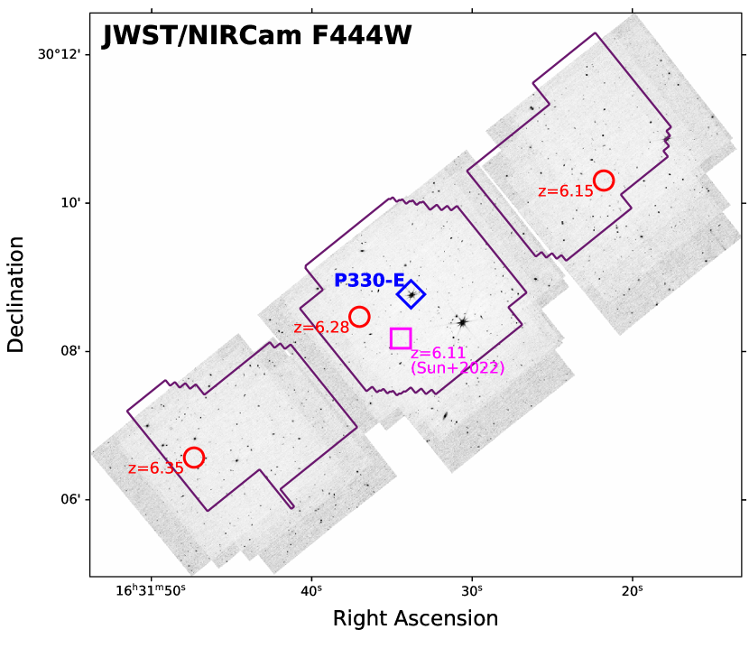
Figure 1: JWST/NIRCam F444W map of the P330-E field. The open blue diamond denotes the primary target (P330-E as the flux calibrator) of the obtained observations. The $z=6.11$ [O III] and H$\alpha$ line emitter discovered by Sun et al. (2022a, Paper I) is shown in the open magenta square, and the three newly discovered [O III] and H$\alpha$ line emitters (this work, $z=6.15-6.35$) are shown in open red circles. The purple contours denote the regions in which sources can potentially yield both [O III] and H$\alpha$ line detections with this survey at $z=6.2$ (see Appendix A).

The JWST/NIRCam long-wavelength (LW; 2.4–5.0 $\mathrm{\SIUnitSymbolMicro m}$) grism characterization observations were conducted through Program #1076 (PI: Pirzkal) during the commissioning phase of the instrument (Rieke et al., 2023; Rigby et al., 2023). Both grism spectroscopic and direct-imaging observations were performed with the flux-calibration star P330-E (a solar analog) and the wavelength-calibration star IRAS 05248-7007 (a post-Asymptotic-Giant-Branch star in the Large Magellanic Cloud). The obtained data were also described in Paper I.

2.1 Direct Imaging

The imaging data of the P330-E field were taken either simultaneously with the grism exposures (short-wavelength, SW filter: F212N) or after the grism observations through direct and out-of-field imaging (SW filter: F212N; LW filter: F250M, F322W2, F335M and F444W). Among them, the shallow F250M and F335M data were taken with the observations #103/104 as part of the early spectral calibration on UT 2022 April 5. The total integration times were 6.4 and 4.3 min (three integrations each), respectively. The F322W2 and F444W imaging data were taken through the observations #105-108 and #109-112, respectively. The total integration time was 4 min (eleven integrations each) with either of the two filters.

For the shallow F212N data, we only used 31 integrations associated with the LW grism exposures because the integrations were longer (96 s each). Shorter F212N integrations (21 s each, 8 min in total) taken with out-of-field imaging were not included because they caused problems for the tweakreg step in jwst Stage-3 mosaicking pipeline in source identification and world-coordinate-system (WCS) registration. The final mosaicked F212N image has a total integration time of 50 min.

The direct-imaging data were reduced and mosaicked using a modified Stage-1/2/3 jwst pipeline 1.8.2 and crds calibration reference file context “jwst_1041.pmap”. This version has included the Cycle-1 NIRCam photometric zero-points (see Boyer et al. 2022 and Rigby et al. 2023). The so-called 1/f noise (see Schlawin et al. 2020) was modeled and removed using the code tshirt/roeba for stage-2 products (i.e., the “_cal.fits” files). The “snowball” artifacts from cosmic rays were identified and masked through their large-area jump-detection information ($\geq$60 native pixels) on the data-quality map of each individual integration. The final image products were resampled to a native pixel size of 0$\farcs$0312 (SW) and 0$\farcs$0629 (LW) with pixfrac $=$ 0.8, and the WCS of the images were registered with the Gaia DR2 catalog (Gaia Collaboration et al., 2018). More specifically, we registered the F444W mosaic image to the Gaia catalog, and then registered the images in all of the other filters to the frame of the F444W image. The mosaicked F444W image of the P330-E field is displayed in Figure 1.

Finally, we performed source extraction with the mosaicked F322W2 and F444W images using SExtractor v2.25.3 (Bertin & Arnouts, 1996) in the single-image detection mode down to $5\sigma$ detection levels. The depths are $\sim$25.5 and 24.9 AB mag in the F322W2 and F444W band, respectively, derived using the automatic Kron aperture and sky background measured from local annulus.

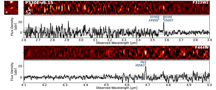
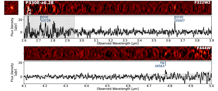
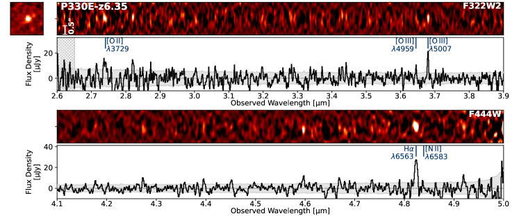
Figure 2: Discovery image and 2D/1D spectra of three [O III] and H$\alpha$ line emitters at $z=6.15$ (top), 6.28 (center) and 6.35 (bottom). In each plot, the NIRCam/F444W cutout image (size: 1$\farcs$9$\times$1$\farcs$9) is shown in the top-left panel. Co-added, calibrated and background-subtracted 2D and 1D spectra in the F322W2 and F444W band are shown on the right. Notable emission lines are labeled with dark blue lines. 1D error spectra are shown as the gray-shaded regions, and wavelength ranges with overlapping continuum contaminants are shown as the gray-hatched regions. Note that the line widths of [O III] and H$\alpha$ are consistent for each source, although they look different in the plot because of different intrinsic aspect ratios of the 2D spectra.

2.2 Grism Spectroscopy

As described in Paper I, the WFSS observations of the P330-E field were obtained with both the F322W2 (2.4–4.0 $\mathrm{\SIUnitSymbolMicro m}$) and F444W (3.9–5.0 $\mathrm{\SIUnitSymbolMicro m}$) filters on UT 2022 April 29. The spectral resolution is $R\sim 1600$ at around 4 $\mathrm{\SIUnitSymbolMicro m}$, and the dispersion is $\sim 1$ $\mathrm{n}\mathrm{m}\,\mathrm{p}\mathrm{i}\mathrm{x}\mathrm{e}\mathrm{l}^{-1}$. In each band, the target was observed with four module (A/B)/grism (R/C; orthogonal) combinations (AR, AC, BR and BC) at four intramodulex primary dither positions, respectively. With the five-group bright1 readout pattern, the effective exposure time per integration was 96 s. Following Paper I, the last integration with the Module B Grism C in the F322W2 band (Observation #108, Visit 001, Exposure 4) was not used in our analysis because of unstable guiding. The maximum exposure time for a source is $\sim$25 min in each band after combining integrations with all grisms. However, we also note that the actual effective exposure time could be shorter, depending on the wavelength of interest and the sky position of the source. Therefore, the median exposure time in each band is $\sim$10 min. We refer the reader to the JWST User Documentation and Rieke et al. (2023) for further information.

The WFSS data were reduced to the level of Stage-1 (i.e., “_rate” files) with the same standard jwst calibration pipeline. We applied a pixel-to-pixel flat-field correction using the imaging flat data obtained with the same filter and module. This is the same method as that we adopted for the F322W2/F444W grism flux calibration during the commissioning of the NIRCam/WFSS mode (also Paper I), because the large-scale grism flat-field calibration has not been complete at the time of writing. In the standard jwst pipeline, the step of grism background subtraction is performed by scaling the theoretical background to that observed in each individual integration. However, the accuracy of the current theoretical background is limited by the accuracy of the sky-background spectrum and the grism tracing/dispersion model (first and second order), neither of which have yet been fully characterized. As in Paper I, we performed the 2D sky-background subtraction using the sigma-clipped median grism images.

Because the dithering of the telescope could introduce astrometric errors (i.e., the dithers might not exactly equal the commanded values), the WCS of each grism image was calibrated with the Gaia DR2 catalog by matching with the stars detected in the NIRCam SW images, which were taken simultaneously in the F212N band. We note that such a registration relies on the internal alignment between NIRCam SW and LW instrument aperture and may introduce astrometric residuals. However, these residuals should be stable and have been included in the grism spectral tracing models.

The grism spectral tracing models, which give the relation between the spectral pixels $(x_{s},y_{s})$ and the direct-imaging position $(x_{0},y_{0})$, were constructed using the spectral traces of point sources observed within the P330-E field. The spectral tracing functions (e.g., $y_{s}(x_{0},y_{0},x_{s})$ in Grism R) were constructed separately for the AR, AC, BR and BC module/grism combinations in the F322W2 and F444W filter. These functions include a third-degree polynomial of $x_{0}$, $y_{0}$ and a second-degree polynomial of $x_{s}$ to fit the strong curvature and field dependence of the spectral traces. With any given spectral pixel position in the dispersion direction (e.g., $x_{s}$ in Grism R), our spectral tracing model can predict the position along the perpendicular direction (e.g., $y_{s}$ in Grism R) with a root-mean-square (RMS) accuracy of 0.1–0.2 pixel, i.e., 10–20% of the RMS width of the point-source spectral trace.

The grism dispersion models, which give the relation between the spectral pixels along the dispersion direction (e.g., $x_{s}$ in Grism R) and $(x_{0},y_{0})$ and wavelength of interest ($\lambda$), were constructed using the emission-line spectra of IRAS 05248–7007. Up to eleven hydrogen recombination lines in Brackett ($n=4$), Pfund ($n=5$) and Humphreys ($n=6$) series were used for wavelength calibration in the F322W2 band, and up to eight lines were used in the F444W band, including hydrogen recombination lines and a He I line at 4.296 $\mathrm{\SIUnitSymbolMicro m}$ (rest frame). The dispersion functions (e.g., $x_{s}(x_{0},y_{0},\lambda)$ in Grism R) were constructed separately for the AR, AC, BR and BC module/grism combinations using the F322W2 and F444W data simultaneously. These functions include a second-degree polynomial of $x_{0}$, $y_{0}$ and a third-degree polynomial of $\lambda$ to perform wavelength calibration with field dependence. Our dispersion model can predict the position of a spectral feature at a wavelength of $\lambda_{s}$ along the dispersion direction (e.g., $x_{s}$ in Grism R) with an RMS accuracy of 0.2 pixel, i.e., $\sim$ 10% of the two-pixel resolution element.

We also used the spectra of P330-E to construct the flux calibration functions in the F322W2 and F444W filters. Using the grism tracing and dispersion models described above, we extracted the spectra of the standard star using box apertures with a height of $D=20$ pixels (1$\farcs$26). The corresponding aperture loss was found to be small (2–3%) when compared with the extracted spectra with a larger aperture ($D=100$ pixels). This loss was corrected in the analyses below. The flux calibration functions, i.e., conversion factors from count rate (unit: DN/s) to flux density (unit: mJy) as functions of wavelength, were constructed using all of the available integrations for four grisms taken in the F322W2 and F444W filters, respectively, with a wavelength step of 0.005 $\mathrm{\SIUnitSymbolMicro m}$ ($\sim 5$ pixels). Through the comparisons of extracted P330-E spectra in different exposures and different locations on the detector, we find that the variations of count rates are only 1–2% when the spectra are binned to 0.005 $\mathrm{\SIUnitSymbolMicro m}$. We therefore conclude that the accuracy of flux calibration is dominated by the systematic uncertainty ($\sim$2% from standard star; Gordon et al. 2022) and flat-field error ($\sim 3$% for pixel variation).

The grism spectral tracing, dispersion and flux calibration models derived from the commissioning data have been made available online. With the derived source catalog in Section 2.1 and models described above, we conducted 2D spectral extraction, wavelength and flux calibration on the flat-fielded WFSS data, and combined the extracted 2D spectra taken with Grism R, C and both. These were performed for $\sim$3000 sources detected in the F322W2 and F444W image as described in Paper I.

3 Results

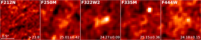
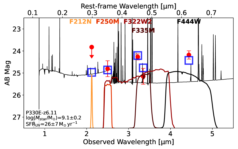
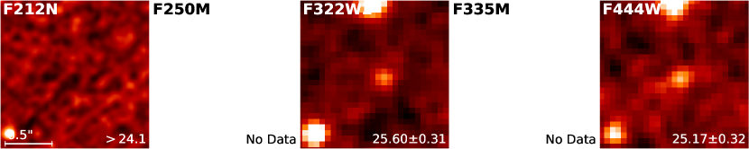
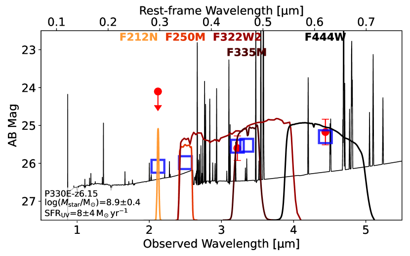
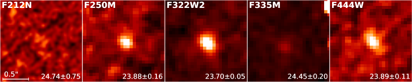
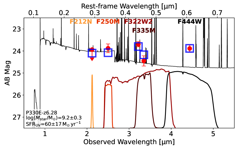
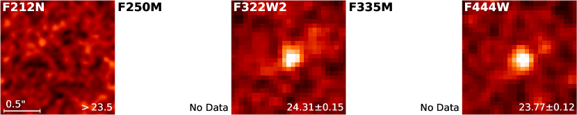
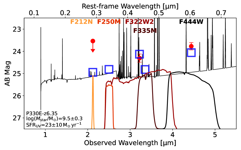
Figure 3: JWST/NIRCam multiple-wavelength cutout images and SED models of the four sources presented in this work. In each panel we show F212N, F250M, F322W2, F335M and F444W cutout images on the top. Measured source brightnesses are shown in the lower-right corner of each cutout image (unit: AB mag; $3\sigma$ upper limit for non-detection). These measurements are shown as filled red circles in the SED plot. Best-fit SED models obtained with cigale are shown as black curve, and best-fit source brightnesses in all filters are shown as open blue squares. The transmission curves of all used filters are also shown for comparison. Derived stellar mass and UV-based SFR are shown in the lower-left corner of each SED plot.

3.1 Discoveries of H$\alpha$$+$[O III] Emitters at $z>6$

We limited the search for line emitters at $z>6$ to a survey area that could yield detections of both [O III] $\lambda$5007 (in the F322W2 band, observed wavelength $\lambda_{\mathrm{obs}}>3.5$ $\mathrm{\SIUnitSymbolMicro m}$) and H$\alpha$ lines (in the F444W band; $\lambda_{\mathrm{obs}}>4.6$ $\mathrm{\SIUnitSymbolMicro m}$). These two emission lines are expected to be the most luminous lines of star-forming galaxies in the rest-frame optical, and the detection of these two lines can securely determine the redshift. The effective survey area, up to 14.4 $\mathrm{a}\mathrm{r}\mathrm{c}\mathrm{m}\mathrm{i}\mathrm{n}^{2}$, depends on the redshift and expected line luminosities, which will be further discussed in Appendix A.

Line emitters were identified through visual inspection of 2D grism spectral images, 1D spectra and 2D direct images taken in both the F322W2 and F444W bands. Because the underlying stellar continuum emission of EoR galaxies is not expected to be detectable with the shallow grism data in the combined 2D spectral images, we subtracted the median-filtered 2D background. The 1D spectra were then optimally extracted (Horne, 1986) based on the Gaussian models of emission-line profiles in the spatial direction. The 1D uncertainty spectra were generated using the error extension of the 2D spectra, and we confirm that they are consistent with the RMS of 1D scientific spectra. All of the line profiles in collapsed 1D spectra were modeled with Gaussian profiles, and potential [O III] and H$\alpha$ emission lines with a signal-to-noise ratio (S/N) that was less than 3 were discarded from further analysis.

Among $\sim$3000 direct-imaging sources detected in either the F322W2 or F444W band, $\sim$10% of them yielded potential emission-line detections (see the $z=4.4$ [O III] and H$\alpha$ line emitter in the JWST commissioning report; Rigby et al. 2023). Four sources were confirmed at $z>6$ after careful inspection, including the $z=6.112$ source reported in Paper I and three new sources at $z=6.146$, 6.279 and 6.348. All of these sources yielded secure [O III] $\lambda$5007 ($>5\sigma$) and H$\alpha$ ($>3\sigma$) line detections in the coadded spectra, which could be detected in both the R and C grism data separately as long as the lines are within the wavelength coverage. These galaxies are referred to as P330E-z6.11, P330E-z6.15, P330E-z6.28 and P330E-z6.35 hereafter based on the ID of the primary target in the field and their redshifts.

Figure 1 shows the locations of these $z>6$ emission-line galaxies in the mosaicked NIRCam F444W map. The cutout direct images, 2D spectra and 1D spectra are shown in Figure 2 with notable emission lines labeled. Among them, P330E-z6.11 and z6.28 were always observed with the flux calibrator in the same module of NIRCam, and therefore their effective integration time is $\sim$20 min with each filter, which is roughly twice that of the other two sources. We also note that a few other suspicious lines can be identified in the 2D spectra, but most of them were only detected in the spectra produced by either the R or C grism, and therefore their associations with the sources are doubtful.

We modeled the properties of detectable emission lines (in increasing order of wavelength: [O II] $\lambda$3727, H$\beta$, [O III] $\lambda\lambda$4959, 5007, H$\alpha$ and [N II] $\lambda$6583) using Gaussian profiles. Among them, H$\beta$+[O III] line profiles were fitted simultaneously, and the line centers were controlled by the redshift parameter. Given the low significance of the detection, the H$\beta$ and [O III] $\lambda$4959 line FWHMs were fixed to be the same as those of the [O III] $\lambda$5007 lines. H$\alpha$$+$[N II] $\lambda$6583 lines were modeled in the same way. The best-fit redshift parameters are consistent with those derived from H$\beta$+[O III] fitting within $\Delta z\sim 0.001$, demonstrating the accuracy of the wavelength calibration. We fitted the flux of the [O II] $\lambda\lambda$3726, 3729 lines using a single Gaussian profile at $\lambda$3727 because the doublet cannot be resolved. In this fit, the redshift parameter was fixed and the line FWHM was set to be identical to the average FWHM of the H$\alpha$ and [O III] lines to mitigate the artificial broadening and flux-boosting effect because of low significance of the line detections (see discussion in Appendix A).

All of the line flux measurements are presented in Table 1. In addition to the firm detections of [O III] $\lambda$5007 and H$\alpha$ lines, [O II] $\lambda$3727 lines were detected in P330E-z6.28/z6.35 at $\sim 2.6\sigma$, which appear to be more luminous than their [O III] $\lambda$5007 lines. H$\beta$ was not detected for the three new sources presented here, while the $3\sigma$ upper limits of line fluxes are consistent with or higher than those estimated from H$\alpha$ line fluxes assuming Case B recombination with a typical electron temperature of $T_{\mathrm{e}}=10^{4}$ K (H$\alpha$/H$\beta$=2.86; Osterbrock & Ferland, 2006). The [O III] $\lambda$4959 lines were also tentatively detected for all sources (up to $3.7\sigma$), and the line ratios to [O III] $\lambda$5007 line are consistent with the theoretical ratio of 1/3. Finally, the significance of [N II] $\lambda$6583 line is $<2\sigma$ for all sources in our sample.

Table 1: Summary of the properties of $z>6$ H$\alpha$ and [O III] emitters in this work.

	P330E-z6.11	P330E-z6.15	P330E-z6.28	P330E-z6.35
R.A.	16:31:34.46	16:31:21.79	16:31:37.02	16:31:47.34
Decl.	+30:08:10.5	+30:10:18.4	+30:08:28.1	+30:06:34.2
Redshift	6.112$\pm$0.001	6.145$\pm$0.001	6.280$\pm$0.001	6.348$\pm$0.001
Photometric Properties
F212N [AB mag]	$>$23.8	$>$24.1	24.74$\pm$0.75	$>$23.5
F250M [AB mag]	25.01$\pm$0.42	$\cdots$	23.88$\pm$0.16	$\cdots$
F322W2 [AB mag]	24.27$\pm$0.09	25.60$\pm$0.31	23.70$\pm$0.05	24.31$\pm$0.15
F335M [AB mag]	25.15$\pm$0.36	$\cdots$	24.45$\pm$0.20	$\cdots$
F444W [AB mag]	24.18$\pm$0.15	25.17$\pm$0.32	23.89$\pm$0.11	23.77$\pm$0.12
Spectroscopic Properties
$f$([O II] $\lambda$3727) [$\mathrm{1}\mathrm{0}^{-18}\,\mathrm{e}\mathrm{r}\mathrm{g}\,\mathrm{s}^{-1}\,\mathrm{c}\mathrm{m}^{-2}$]	$<$30.9	$<$52.3	22.2$\pm$9.5	30.7$\pm$10.9
$f$(H$\beta$) [$\mathrm{1}\mathrm{0}^{-18}\,\mathrm{e}\mathrm{r}\mathrm{g}\,\mathrm{s}^{-1}\,\mathrm{c}\mathrm{m}^{-2}$]	7.1$\pm$2.8	$<$15.6	$<$5.2	$<$9.6
$f$([O III] $\lambda$4959) [$\mathrm{1}\mathrm{0}^{-18}\,\mathrm{e}\mathrm{r}\mathrm{g}\,\mathrm{s}^{-1}\,\mathrm{c}\mathrm{m}^{-2}$]	9.9$\pm$2.7	7.3$\pm$3.6	2.1$\pm$1.7	8.7$\pm$3.1
$f$([O III] $\lambda$5007) [$\mathrm{1}\mathrm{0}^{-18}\,\mathrm{e}\mathrm{r}\mathrm{g}\,\mathrm{s}^{-1}\,\mathrm{c}\mathrm{m}^{-2}$]	34.8$\pm$3.2	24.8$\pm$4.1	13.8$\pm$2.1	20.9$\pm$3.6
$f$(H$\alpha$) [$\mathrm{1}\mathrm{0}^{-18}\,\mathrm{e}\mathrm{r}\mathrm{g}\,\mathrm{s}^{-1}\,\mathrm{c}\mathrm{m}^{-2}$]	14.7$\pm$2.6	16.9$\pm$3.2	7.6$\pm$2.3	26.5$\pm$3.8
$f$([N II] $\lambda$6583) [$\mathrm{1}\mathrm{0}^{-18}\,\mathrm{e}\mathrm{r}\mathrm{g}\,\mathrm{s}^{-1}\,\mathrm{c}\mathrm{m}^{-2}$]	$<$6.3	$<$7.0	$<$5.8	3.6$\pm$2.9
EW([O II] $\lambda$3727) [Å]	$<$213	$\cdots$	97$\pm$45	291$\pm$114
EW(H$\beta$) [Å]	70$\pm$29	$<$729	$<$35	$<$94
EW([O III] $\lambda$4959) [Å]	100$\pm$30	344$\pm$254	14$\pm$12	85$\pm$33
EW([O III] $\lambda$5007) [Å]	359$\pm$60	1165$\pm$670	97$\pm$22	205$\pm$49
EW(H$\alpha$) [Å]	221$\pm$50	841$\pm$489	84$\pm$29	267$\pm$59
EW([N II] $\lambda$6583) [Å]	$<$96	$<$353	$<$63	36$\pm$30
Physical Properties
$\log[M_{\mathrm{star}}/\mbox{$\mathrm{M}_{\odot}$}]$	9.1$\pm$0.2	8.9$\pm$0.4	9.2$\pm$0.3	9.5$\pm$0.3
SFR(H$\alpha$) [$\mathrm{M}_{\odot}\,\mathrm{y}\mathrm{r}^{-1}$]	32$\pm$5	38$\pm$7	18$\pm$5	64$\pm$9
SFR(SED,UV) [$\mathrm{M}_{\odot}\,\mathrm{y}\mathrm{r}^{-1}$]	25$\pm$7	7$\pm$4	60$\pm$17	22$\pm$10
$\log[\xi_{\mathrm{ion}}/(\mathrm{erg}^{-1}\mathrm{Hz})]$	25.2$\pm$0.1	25.8$\pm$0.3	24.6$\pm$0.2	25.5$\pm$0.2
12 + $\log$(O/H)	8.2$\pm$0.2	8.3$\pm$0.2	8.2$\pm$0.3	8.4$\pm$0.2

3.2 Photometry and Line Equivalent Widths

Similar to Paper I, we performed aperture photometry of all $z>6$ line-emitting galaxies in F212N, F250M, F322W2, F335M and F444W band. Unlike P330E-z6.11 that has a clear two-component structure, the three new sources found in this work were detected as single-component systems and their angular sizes are generally compact (FWHM $\lesssim$ 0$\farcs$25). We adopted a conservative circular aperture of $r=0\farcs 45$ using photutils (Bradley et al., 2020) to avoid missing extended components and minimize the aperture loss, similar to that used in Paper I. With such an aperture radius, the variation of the encircled light fractions of point spread functions at 2–5 $\mathrm{\SIUnitSymbolMicro m}$ is $\sim$3%, much smaller than the photometric uncertainty. We also modeled the F444W surface brightness profiles of sources in our sample with the 2D Gaussian model, and we confirmed that the aperture loss is negligible. We subtracted the sky background using the median of sigma-clipped local annulus, and computed the photometric uncertainty using the RMS of that. Broad-band photometry is summarized in Table 1.

All sources were detected in the broad F322W2 and F444W bands, but remained undetected within the narrow F212N filter. For P330E-z6.28 with the F250M and F335M coverage, we were able to detect its rest-frame UV continuum (23.88$\pm$0.16 AB mag in the F250M band) and optical stellar continuum (24.45$\pm$0.20 AB mag in the F335M band). At this redshift, no strong emission line is expected in the wavelength range of the F250M and F335M filters, but the flux densities measured with the broad F322W2 and F444W filters could be boosted by strong [O III] and H$\alpha$ lines, respectively. Indeed, we find a blue F250M–F335M color of $-0.57\pm 0.26$ and an F322W2–F335M excess of $0.75\pm 0.21$ mag, both suggesting the presence of strong nebular emission lines (e.g., [O III]) and potentially nebular continuum blueward of the Balmer break ($\lambda_{\mathrm{rest}}<3640$ Å).

With the continuum photometry, we computed the line equivalent widths (EWs). To estimate the underlying continuum flux density, we subtracted all measured line fluxes within the passband for all broad-band photometric measurements redward of the Balmer break (F322W2, F444W and F335M if available). The continuum flux densities were then modeled with a power-law function $f_{\mathrm{\nu}}\propto\lambda^{\alpha}$. We then computed the line EW using the underlying continuum strength estimated at the line wavelength. All of the line EWs are reported in Table 1. However, we also note that the broad-band flux density could be slightly overestimated because of the contribution from undetected faint emission lines that may not have been properly subtracted, which could potentially lead to underestimates in line EWs. The Balmer discontinuity can also introduce errors into the continuum flux density determination in the F322W2 band.

4 Discussion I: Physical Properties

4.1 SED modeling

To derive the physical properties of galaxies in our sample, we perform SED modeling with cigale (Boquien et al., 2019). Broad-band photometry and the EWs of [O III] and H$\alpha$ lines are included as constraints. [O II], H$\beta$ and [N II] line EWs are not included given the general low significance of detections. Similar to that in Paper I, we assume a commonly used delayed star-formation history (SFH; sfhdelayed), in which $\mathrm{SFR}(t)\propto t\exp(-t/\tau)$ and $\tau$ is the peak time of SFH. An optional late starburst is allowed in the last 1–5 Myr, which can contribute to 0–80% of the total stellar mass. We use Bruzual & Charlot (2003) stellar population synthesis models. We also allow a metallicity range of 0.2 $\mathrm{Z}_{\odot}$ to $\mathrm{Z}_{\odot}$, a broad ionization parameter ($\log U$) range of $-1.0$ to $-3.5$. We adopt the Calzetti et al. (2000) attenuation curve and the color excess of the nebular lines is allowed between $E(B-V)_{\mathrm{line}}=0-1$.

The best-fit SED models are shown in Figure 3. The best-fit SEDs are rich in emission lines, indicating that the galaxies are young and star-forming. However, most of the lines are too faint to be detected in the grism spectra.. Similar to the results in Paper I, the best-fit SFH models typically invoke both a young (1–2 Myr) and old ($\sim 300$ Myr) stellar populations. Roughly half of the stellar masses in all galaxies are produced by the most recent starburst, which is consistent with the presence of strong nebular emission lines. We note that this result is driven by the large emission-line EWs. If the fitting is performed without line EWs, then the amount of recent star formation will decrease sharply.

The median mass-weighted stellar age of sources in our sample is $74\pm 50$ Myr, and the median stellar mass ($M_{\mathrm{star}}$) is $1.4_{-0.5}^{+0.7}\times 10^{9}$ $\mathrm{M}_{\odot}$. Dust attenuation is negligible for P330E-z6.11/6.28, which is likely not the case for P330E-z6.15 ($A_{V}=1.1\pm 0.7$ for stellar continuum) and P330E-z6.35 ($A_{V}=1.4\pm 0.7$) as indicated by their red F322W2–F444W colors even after the subtraction of [O III] and H$\alpha$ lines. However, we also note that the constraints on the dust attenuation and stellar masses are not tight, given that three of the sources were only detected in the two broad LW bands.

The derived physical properties of galaxies in our sample are also presented in Table 1. The physical properties of P330E-z6.11 have been reported in Paper I, and we have updated our results with the latest flux calibration. The differences from those in Paper I are small, within $1\sigma$ significance level. Following Paper I, we also infer UV SFRs for galaxies in our sample from the best-fit SED, and the median is $24\pm 11$ $\mathrm{M}_{\odot}\,\mathrm{y}\mathrm{r}^{-1}$. This is smaller than the median of H$\alpha$-based SFR ($35\pm 9$ $\mathrm{M}_{\odot}\,\mathrm{y}\mathrm{r}^{-1}$) assuming the conversion in Kennicutt & Evans (2012, uncorrected for dust attenuation). This comparison likely indicates (i) a bursting nature because H$\alpha$ is more sensitive to the most recent star formation than UV continuum (see Kennicutt & Evans 2012), (ii) a higher ionizing photon production efficiency ($\xi_{\mathrm{ion}}$), lower metallicity and thus smaller H$\alpha$/SFR conversion factor (e.g., Charlot et al., 2002; Brinchmann et al., 2004) at high redshift when compared with the local Universe, and (iii) a higher dust extinction in the rest-frame UV than with the H$\alpha$ line (see further discussions in Section 4.5).

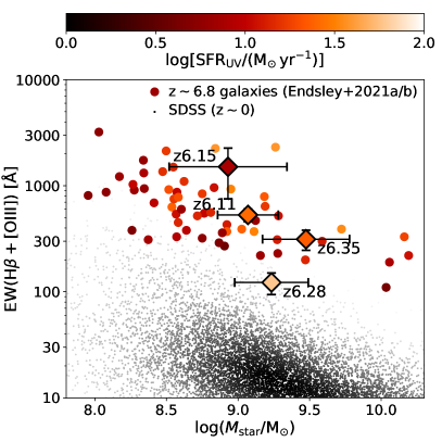
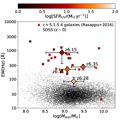
Figure 4: Left: H$\beta$$+$[O III] EWs versus stellar masses of sources in our sample (diamonds), compared with galaxies at $z\sim 6.8$ whose line EWs are inferred from Spitzer/IRAC [3.6]–[4.5] $\mathrm{\SIUnitSymbolMicro m}$ colors (circles; Endsley et al. 2021a, b). Right: H$\alpha$ EWs versus stellar masses of sources in our sample (diamonds), compared with galaxies at $z\simeq 5.1-5.4$ whose line EWs are also inferred from IRAC colors (squares; Rasappu et al. 2016). In both panels, all high-redshift sources are color-coded by their UV-based SFRs. SDSS-selected galaxies in the local Universe are also shown as dots for comparison.

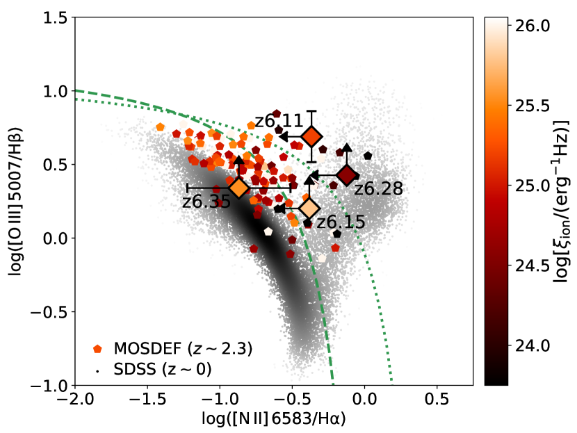
Figure 5: [O III]/H$\beta$–[N II]/H$\alpha$ BPT diagram of $z>6$ galaxies in our sample (diamonds), compared with those of $z\sim 2.3$ emission-line galaxies in MOSDEF sample (pentagons; Kriek et al., 2015; Reddy et al., 2015; Shapley et al., 2015). Galaxies in both samples are color-coded by their ionizing photon production efficiencies, and likely occupy the same parameter space. SDSS-selected galaxies and AGN in the local Universe are shown as dots in background, color-coded by their number densities in the parameter space. The dotted green line is the so-called “maximum-starburst” line in Kewley et al. (2001), and the dashed green line is the canonical AGN/star-forming galaxy boundary in Kauffmann et al. (2003a).

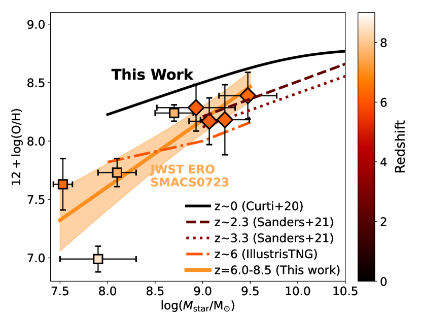
Figure 6: Gas-phase metallicity versus stellar mass of $z>6$ galaxies in our sample (diamonds; measured using various strong line ratios calibrated by Bian et al. 2018), compared with those obtained with JWST/NIRSpec early-release observations in SMACSJ0723 field (squares; Curti et al. 2023, Taylor et al. 2022) measured using the direct $T_{\mathrm{e}}$ method. The best-fit mass-metallicity relation of $z>6$ galaxies is shown as solid orange line, with $1\sigma$ uncertainty shown as shallower filled region. We also compare our measurements with those of SDSS galaxies in the local Universe (Curti et al., 2020), and $z\sim 2.3$ and 3.3 galaxies in the MOSDEF sample (Sanders et al. 2021; also based on Bian et al. 2018 calibration). Mass-metallicity relation at $z\sim 6$ in the IllustrisTNG simulation (Torrey et al., 2019) is also shown for comparisons (dash-dotted orange-red line). All samples and relations shown in this plot are color-coded by the redshifts.

4.2 Comparison of Line EWs with $z\simeq 5-7$ galaxies

Before the launch of the JWST, the EWs of strong [O III] and H$\alpha$ emission lines at high redshifts were modeled from Spitzer/IRAC photometry. In this section, we compare the line EWs of galaxies in our sample, derived from rest-frame optical spectroscopy, with those inferred previously from the IRAC SED analyses.

In the left panel of Figure 4, we compare the [O III]$+$H$\beta$ line EWs and stellar masses with those of $z\sim 6.8$ galaxies in Endsley et al. (2021a, b). The median [O III]$+$H$\beta$ line EW of the sources in our sample is 416$\pm$66 Å, with the maximum and minimum of 1510$\pm$757 Å (P330E-z6.15) and 122$\pm$28 Å (P330E-z6.28), respectively. Before the launch of JWST, [O III]$+$H$\beta$ line EWs at $z\gtrsim 4$ could only be inferred from Spitzer/IRAC SED analysis in certain redshift windows, for example, $z\simeq 6.7-7.0$ (e.g., Smit et al., 2014, 2015; Endsley et al., 2021a, b). Endsley et al. (2021b) reported a median [O III]$+$H$\beta$ EW of $759_{-113}^{+112}$ Å for a sample of UV-bright ($M_{\mathrm{UV}}\lesssim-21$) galaxies at $z\sim 6.8$, and the scatter is $\sim$ 0.25 dex.

Through a Kolmogorov–Smirnov test, we confirm that the [O III]$+$H$\beta$ line EW distribution of the sources in our sample is consistent with that in Endsley et al. (2021a, b) over a similar stellar-mass ($\sim 10^{9}$ $\mathrm{M}_{\odot}$) and SFR ($\gtrsim 10$ $\mathrm{M}_{\odot}\,\mathrm{y}\mathrm{r}^{-1}$) range. Similar to the findings in Paper I, this confirms the presence of strong rest-frame optical nebular emission lines in EoR galaxies with a wide range of line EWs ($\sim$1 dex span). Such a wide span is also seen with certain simulations (e.g. Ceverino et al., 2021).

We derive a median H$\alpha$ EW of 239$\pm$45 Å for the galaxies in our sample with a maximum and minimum of 814$\pm$489 Å (P330E-z6.15) and 84$\pm$29 Å (P330E-z6.28), respectively. We also compare the H$\alpha$ EWs with those of $z\simeq 5.1-5.4$ galaxies reported in Rasappu et al. (2016), whose line EWs were inferred from Spitzer/IRAC SEDs. In this redshift window, the H$\alpha$ lines enter the passband of IRAC Channel 2 (CH2; 4.5 $\mathrm{\SIUnitSymbolMicro m}$), while the Channel 1 (CH1, 3.6 $\mathrm{\SIUnitSymbolMicro m}$) is free from strong emission lines including H$\beta$ and [O III] ($\lambda<3.2$ $\mathrm{\SIUnitSymbolMicro m}$). Therefore, a red [3.6]–[4.5] color can be used to infer the strength of H$\alpha$ emission. We assumed that $\sim$ 80% of the combined H$\alpha$+[N II]+[S II] EWs reported in Rasappu et al. (2016) is from H$\alpha$, similar to the fraction assumed in their work (84%; from Anders & Fritze-v. Alvensleben 2003).

With comparable stellar masses and SFRs, the median H$\alpha$ EW of the galaxies with spectroscopic redshifts in Rasappu et al. (2016) is $564\pm 59$ Å, $2.4\pm 0.5$ times that for our sample. Although this can be potentially explained by the limited understanding of dust extinction and underlying stellar continuum in early Spitzer/IRAC studies, we cannot draw any firm conclusion from the H$\alpha$ EW comparison given the small sample size.

Finally, we also compare the line EWs with those of galaxies in the local Universe with comparable stellar masses. We select galaxies at $z<0.05$ from the MPA-JHU value-added catalog of SDSS Data Release 7 (Kauffmann et al., 2003b; Abazajian et al., 2009) for comparison (black dots in Figure 4). The EWs of H$\alpha$ and [O III] lines of galaxies in our sample are higher than the median EWs of SDSS-selected galaxies by at least an order of magnitude. Our conclusion remains valid if we compared with galaxies in the Portsmouth SDSS catalog (Maraston et al., 2013; Thomas et al., 2013).

4.3 Line Ratios and BPT Diagram

Despite secure identification of [O III] and H$\alpha$ lines, the sources in our sample are typically undetected in either [N II] $\lambda$6583 or H$\beta$ lines. With the latest calibrated spectra, the H$\beta$ line of P330E-z6.11 is detected at 2.5$\sigma$, suggesting a line ratio of [O III]/H$\beta$ $=4.9\pm 1.3$. None of the sources are detected in [N II] $\lambda$6583 at above $2\sigma$, and thus the typical $3\sigma$ upper limit of [N II]/H$\alpha$ line ratio is $<0.4$.

With these line ratios and upper/lower limits, we plot our sources on the [O III]/H$\beta$-[N II]/H$\alpha$ BPT diagram (Baldwin et al., 1981) in Figure 5. We compare our sample with galaxies in the local Universe (in the MPA-JHU catalog for SDSS Data Release 7; Abazajian et al., 2009) and $z\sim 2.3$ galaxies in the MOSDEF sample (Kriek et al., 2015; Reddy et al., 2015; Shapley et al., 2015). Although the detection rate of H$\beta$ and [N II] lines is low, the $z>6$ emission-line galaxies in our sample appear to occupy the same parameter space as that of $z\sim 2$ star-forming galaxies in the MOSDEF sample, and are likely located above the star-forming sequence of SDSS galaxies (see also recent studies with NIRSpec, e.g., Cameron et al. 2023 and Sanders et al. 2023a). Similar to $z\sim 2$ galaxies, this could be explained by an elevated N/O abundance at a given O/H ratio and/or a higher ionization parameter (e.g., Kewley et al., 2013; Masters et al., 2014; Steidel et al., 2014; Shapley et al., 2015; Kojima et al., 2017; Curti et al., 2022) for high-redshift galaxies with moderate stellar masses ($<10^{10}$ $\mathrm{M}_{\odot}$). Stars that are enhanced in alpha elements can have harder intrinsic ionization spectra, which can lead to a higher [O III]/H$\beta$ at fixed [N II]/H$\alpha$ in nebulae (e.g., Strom et al., 2017; Topping et al., 2020a, b).

It is possible that sources in our sample may contain active galactic nuclei (AGN). However, based on their locations on the BPT diagram (Kewley et al., 2001; Kauffmann et al., 2003a), hydrogen line profiles and number density (Section 5), we do not find strong evidence to confirm any source as AGN.

4.4 Gas-Phase Metallicity

With oxygen and hydrogen lines detected for all sources in our sample, we study their gas-phase metallicity using the strong-line calibrations of Bian et al. (2018). Bian et al. (2018) studied the stacked spectra of local analogs of $z\sim 2$ star-forming galaxies, derived direct gas-phase O/H abundances using [O III] $\lambda$4363 lines, and established empirical metallicity calibrations between O/H abundances and strong-line ratios such as [N II] $\lambda$6583/H$\alpha$ (also known as N2), [O III] $\lambda$5007/H$\beta$, ([O III] $\lambda\lambda$4959,5007$+$[O II] $\lambda$3727)/H$\beta$ (also known as R23) and [O III] $\lambda\lambda$4959,5007/[O II] $\lambda$3727 (also known as O32). Given the similarity of the locations in the [O III]/H$\beta$–[N II]/H$\alpha$ BPT diagram (Figure 5) among our sample, $z\sim 2$ star-forming galaxies and the local analogs analyzed in Bian et al. (2018), these empirical calibrations are likely useful for these galaxies at $z>6$. In the absence of statistical samples of strong line ratios above $z>3$, an estimate using the $z=0-2$ calibrations can provide a valuable first look, but we also make the caveat clear that the empirical calibration may break down in this unexplored redshift regime (e.g., see discussions in Curti et al. 2023 and most recently Sanders et al. 2023b). This is possibly because of the different ISM conditions and physical properties (e.g. N/O, ionization parameter, hardness of the ionizing radiation; Steidel et al. 2016, Strom et al. 2017) of high-redshift galaxies relative to the calibration samples at lower redshifts (Brinchmann, 2022).

We derive the gas-phase metallicity of each source by averaging the measurements with multiple tracers, including N2 (P330E-z6.35), R23 (P330E-z6.28 and P330E-z6.35) and [O III]/H$\beta$ (O3; all sources). For sources without H$\beta$ detections, we assume an intrinsic H$\alpha$/H$\beta$ ratio of 2.86 (case-B recombination and electron temperature of $10^{4}$ K). One caveat is that the H$\alpha$/H$\beta$ ratio could be underestimated because of the dust extinction, and the resultant O/H abundance could be overestimated by 0.2 dex if the H$\alpha$/H$\beta$ ratio is 4. We estimated the uncertainty of metallicity from both the errors of line ratios and the scattering of measurements with multiple tracers. The derived gas-phase metallicities are reported in Table 1. In general, the galaxies in our sample have been enriched to moderate metallicities ($\sim$0.4 $\mathrm{Z}_{\odot}$).

Figure 6 shows the metallicities versus stellar masses of sources in our sample at $z>6$. We also compare our measurements with those of the four $z>6$ galaxies observed through the JWST/NIRSpec ERO of the SMACS0723 field (Pontoppidan et al., 2022). For three sources at $z>7$, we adopt the stellar mass measurements from Tacchella et al. (2022, see also ) and gas-phase metallicities from Curti et al. (2023) using the direct $T_{\mathrm{e}}$ method. For the $z=6.38$ galaxy, we adopt the $M_{\mathrm{star}}$ from Carnall et al. (2023) and $12+\log(\mathrm{O/H})$ from Taylor et al. (2022). We also note that metallicity measurements from Rhoads et al. (2023), Schaerer et al. (2022), Tacchella et al. (2022) and Trump et al. (2023) are in general agreement (Brinchmann, 2022). With higher stellar masses and slightly lower redshift, galaxies in our sample exhibit higher metallicities than those of the four $z>6$ galaxies in the SMACS0723 field. The best-fit mass-metallicity (gas-phase) relation from these eight sources at $z=6.0-8.5$ is:

$$12+\log(\mathrm{O/H})=(0.57\pm 0.16)\log(\frac{M_{\mathrm{star}}}{10^{9}\,\mbox{$\mathrm{M}_{\odot}$}})+8.18\pm 0.12$$ (1)

which is shown as the solid orange line in Figure 6 with the lighter filled region indicating the $1\sigma$ uncertainty range.

Within the investigated stellar mass range ($M_{\mathrm{star}}=10^{7.5}\sim 10^{9.5}$ $\mathrm{M}_{\odot}$), our best-fit relation suggests a lower metallicity at a given stellar mass when compared with $z\sim 0$ galaxies observed with SDSS (e.g., Curti et al. 2020). However, four galaxies in our sample exhibit moderate metallicities that are comparable to those of $z\simeq 2-3$ galaxies in the MOSDEF sample (Sanders et al., 2021), whose metallicities were also derived based on the Bian et al. (2018) calibration. The observed metallicities of sources in our sample are slightly higher than those of galaxies with similar stellar masses in certain cosmological simulations including IllustrisTNG (Torrey et al., 2019). As a result, the best-fit mass-metallicity relation at $z>6$ with JWST is also steeper than that in IllustrisTNG.

However, we note that the slope of the mass-metallicity relation flattens to $0.41\pm 0.07$ if the $z=8.5$ source with extremely low metallicity ($12+\log(\mathrm{O/H})=7.0\pm 0.1$; Curti et al. 2023) in JWST/NIRSpec ERO is excluded from the linear fitting, making the slope closer to those seen at $z\simeq 2-3$ ($\sim 0.30$, Sanders et al. 2021; see also Li et al. 2022 most recently). We also note that to fully explore the evolution with respect to low-redshift galaxies and compare with simulations, one should also consider the secondary dependence of metallicity on SFR (i.e., the fundamental metallicity relation, see discussion in Curti et al. 2023). This additional step is beyond the scope of this paper.

Our observations may indicate a rapid metal enrichment in certain massive ($M_{\mathrm{star}}\gtrsim 10^{9}$ $\mathrm{M}_{\odot}$) galaxies at $z>6$, which is also suggested by the [O III] 88 $\mathrm{\SIUnitSymbolMicro m}$ and dust detections of $z>8$ galaxies with ALMA (Tamura et al. 2019; see also Jones et al. 2020). The enhanced gas-phase metallicity potentially indicates that the recent increase in SFR is driven by mergers or internal gravitational instabilities (e.g., Tacchella et al., 2022) instead of pristine gas inflow, which can result in lower gas-phase metallicity. Such ancient and rapid metallicity evolution and intense episode of star formation is also in a sense reminiscent of the formation scenario of our own Milky Way Bulge, which indeed rapidly evolved toward solar metallicity and formed most of stellar mass $>10$ Gyr ago. However, we also note that our metallicity measurements are totally based on the low-redshift strong-line calibrations, mostly in the metallicity range of $7.8<12+\log(\mathrm{O/H})<8.4$ (Bian et al., 2018). Further direct gas-phase metallicity measurements through JWST/NIRSpec observations (e.g., most recently with Nakajima et al. 2023 and Sanders et al. 2023b) are necessary for more accurate determination of the mass-metallicity relation in the high-redshift Universe.

4.5 Redshift Evolution of H$\alpha$ line Equivalent Width

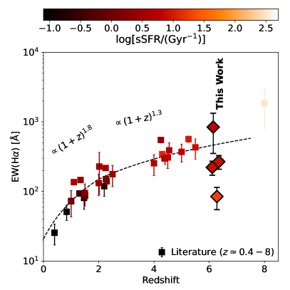
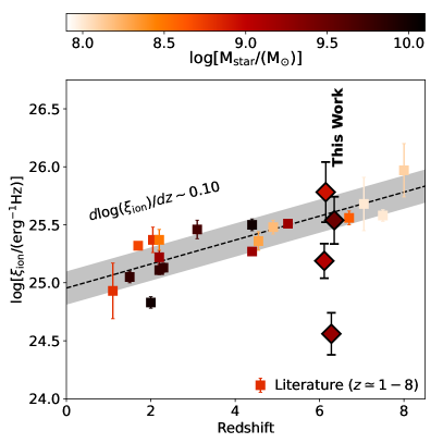
Figure 7: Redshift evolution of H$\alpha$ equivalent widths (left) and ionizing photon production efficiency (right) of star-forming galaxies across $z\simeq 0.4-8$. Sources in our sample are shown as diamonds. In the left panel, the reference samples (squares) include Erb et al. (2006), Shim et al. (2011), Fumagalli et al. (2012), Stark et al. (2013), Sobral et al. (2014), Faisst et al. (2016), Mármol-Queraltó et al. (2016), Rasappu et al. (2016), Smit et al. (2016), Reddy et al. (2018), Lam et al. (2019), Atek et al. (2022), Boyett et al. (2022) and Stefanon et al. (2022), and all samples are color-coded by their specific SFRs. The proposed redshift evolution ($\mathrm{EW}\propto(1+z)^{1.8}$ at $z<2$ and $\propto(1+z)^{1.3}$ beyond) in Faisst et al. (2016) is shown as the dashed black line. In the right panel, the reference samples (squares) include Stark et al. (2015, 2017), Bouwens et al. (2016a), Nakajima et al. (2016), Matthee et al. (2017), Harikane et al. (2018), Shivaei et al. (2018), Faisst et al. (2019), Lam et al. (2019), Tang et al. (2019), Emami et al. (2020), Nanayakkara et al. (2020), Endsley et al. (2021a), Atek et al. (2022) and Stefanon et al. (2022), and all samples are color-coded by their stellar masses. The best-fit redshift evolution ($d\log\xi_{\mathrm{ion}}/dz=0.10\pm 0.02$) of literature samples is shown as the dashed black line, and the $1\sigma$ dispersion of the relation (0.14 dex) is indicated by the shaded gray region.

Before the launch of the JWST, the H$\alpha$ EWs at $z\sim 6$ were poorly probed because [O III] and H$\alpha$ lines are in the bandwidth of IRAC Channel 1 and 2, respectively. In the left panel of Figure 7, we examine the redshift evolution of H$\alpha$ EWs of galaxies from $z\simeq 0.5$ to 8 in the literature. For H$\alpha$ EW measurements obtained with medium/high-resolution spectroscopy (e.g., Erb et al., 2006; Reddy et al., 2018), we directly use the reported EWs. For measurements with low-resolution grism spectroscopy (e.g., Fumagalli et al., 2012; Atek et al., 2022; Boyett et al., 2022) or narrow-band imaging (Sobral et al., 2014) in which H$\alpha$ lines are blended with [N II] lines, we assume that 85% of the line fluxes are from H$\alpha$, consistent with our [N II]/H$\alpha$ measurements in Section 4.3 (see also recent JWST studies, e.g., Cameron et al. 2023, Helton et al. 2023 and Sanders et al. 2023a). For measurements relying on broad-band photometry and SED modeling (e.g., Shim et al., 2011; Stark et al., 2013; Mármol-Queraltó et al., 2016; Rasappu et al., 2016; Smit et al., 2016; Lam et al., 2019; Stefanon et al., 2022), we assume that 80% of H$\alpha$$+$[N II]$+$[S II] line fluxes are from H$\alpha$, consistent with the fractions adopted by various studies (71–84%; e.g., Shim et al. 2011, Rasappu et al. 2016).

The redshift evolution of H$\alpha$ EWs has been described with $\mathrm{EW}\propto(1+z)^{1.8}$ at $z\lesssim 2$ (e.g., Fumagalli et al. 2012) and $\propto(1+z)^{1.3}$ at $z>2$ (Faisst et al., 2016). At $z>2.5$, all H$\alpha$ EWs published before the JWST were derived based on Spitzer/IRAC broad-band colors, and therefore are inevitably affected by multiple uncertainties, including the assumption of SFH and dust attenuation. The median EW(H$\alpha$) of sources in our sample is indeed higher than those of $z\lesssim 2$ galaxies with direct spectroscopic measurements and similar to the previous estimates at $z\simeq 4-5$ (e.g., Shim et al., 2011; Stark et al., 2013; Faisst et al., 2016; Mármol-Queraltó et al., 2016; Rasappu et al., 2016; Smit et al., 2016; Lam et al., 2019). This is likely a fair comparison because the specific SFRs (sSFR; SFR per unit $M_{\mathrm{star}}$) of these samples are comparable. Note that the H$\alpha$ EWs broadly reflect the sSFR’s of galaxies because H$\alpha$ is a SFR tracer while the underlying continuum is related to the luminous stellar mass. However, as the redshifts of galaxies in our sample are higher than those measured with Spitzer/IRAC [3.6]–[4.5] color, this may indicate that the redshift evolution of the H$\alpha$ EWs is flattening toward the EoR, although the robustness of our conclusion is limited by the small sample size. Finally, our H$\alpha$ EW measurements are much lower than that of stacked $z\sim 8$ galaxies ($\sim 2\times 10^{3}$ Å) as inferred from Spitzer/IRAC [3.6]–[5.8] color (Stefanon et al., 2022) despite a large uncertainty.

4.6 Redshift Evolution of $\xi_{\mathrm{ion}}$

Following a few studies including Matthee et al. (2017), Shivaei et al. (2018), Tang et al. (2019) and many others, we derive the ionizing photon production efficiency in H II regions as $\xi_{\mathrm{ion}}=N(\mathrm{H}^{0})/L_{\mathrm{UV}}$, where $N(\mathrm{H}^{0})$ is the ionizing photon production rate in the unit of $\mathrm{s}^{-1}$, and $L_{\mathrm{UV}}$ is the rest-frame UV luminosity at 1500 Å in the unit of $\mathrm{e}\mathrm{r}\mathrm{g}\,\mathrm{s}^{-1}\,\mathrm{H}\mathrm{z}^{-1}$. The ionizing photon production rate can be computed from the H$\alpha$ luminosity as $N(\mathrm{H}^{0})=7.35\times 10^{11}L_{\mathrm{H\alpha}}$ where $L_{\mathrm{H\alpha}}$ is in the unit of $\mathrm{e}\mathrm{r}\mathrm{g}\,\mathrm{s}^{-1}$ (Osterbrock & Ferland 2006; Case B recombination at $T_{\mathrm{e}}=10^{4}$ K). This is true assuming that the Lyman continuum escape fraction is low ($\lesssim 10$%). Note, however, that we do not have near-infrared (1.0–2.2 $\mathrm{\SIUnitSymbolMicro m}$) photometry for our galaxies sampling the rest-frame UV continuum, and therefore we estimate the rest-frame UV luminosities based on the cigale modeling performed in the rest-frame optical as already described.

The median derived $\log[\xi_{\mathrm{ion}}/(\mathrm{erg}^{-1}\,\mathrm{Hz})]$ of galaxies in our sample is $25.4\pm 0.2$, higher than the canonical value of $\sim 25.1$ implied by the UV–SFR and H$\alpha$–SFR conversion in Kennicutt & Evans (2012). However, a stronger dust attenuation in the rest-frame UV could lead to an overestimate of $\xi_{\mathrm{ion}}$. Assuming Calzetti et al. (2000) extinction law, with an $A_{V}=1.0$ and a canonical $E(B-V)$ ratio of 0.44 between stellar continuum and nebular lines, $\xi_{\mathrm{ion}}$ would be overestimated by 1.9 times if the dust attenuation is not properly corrected (see also Shivaei et al. 2018).

In the right panel of Figure 7, we study the redshift evolution of the ionization photon production efficiency. The published samples at $z\simeq 1-8$ include Stark et al. (2015, 2017), Bouwens et al. (2016a), Nakajima et al. (2016), Matthee et al. (2017), Harikane et al. (2018), Shivaei et al. (2018), Faisst et al. (2019), Lam et al. (2019), Tang et al. (2019), Emami et al. (2020), Nanayakkara et al. (2020), Endsley et al. (2021a), Atek et al. (2022) and Stefanon et al. (2022). The stellar mass range of the reference sample is $M_{\mathrm{star}}\simeq 10^{8}-10^{10}$ $\mathrm{M}_{\odot}$, comparable to that of our sample except for those at very high redshifts ($z>7$). Despite a considerable uncertainty of UV luminosity (because we rely on best-fit SED models) and dust attenuation, the $\xi_{\mathrm{ion}}$ measured in this work based on accurate H$\alpha$ luminosity is consistent with the previous determination at $z\simeq 5-7$ (e.g., Stark et al. 2015, Harikane et al. 2018, Endsley et al. 2021a and most recently Ning et al. 2023 and Tang et al. 2023).

As shown by the dashed black line in the plot, the published samples indicate a redshift evolution of $\xi_{\mathrm{ion}}$ with a slope of $d\log(\xi_{\mathrm{ion}})/dz=0.10\pm 0.02$ (see also Matthee et al. 2017, Atek et al. 2022 and Stefanon et al. 2022). This redshift evolution can be interpreted by an age effect, i.e., galaxies at higher redshifts have younger stellar populations therefore higher $\xi_{\mathrm{ion}}$ (e.g., Tacchella et al., 2018; Naidu et al., 2020). The galaxies in our sample are in general agreement with such a redshift evolution trend except for P330E-z6.28 ($\log[\xi_{\mathrm{ion}}/(\mathrm{erg}^{-1}\mathrm{Hz})]=24.6\pm 0.2$). The large scatter of $\log(\xi_{\mathrm{ion}})$ in our sample (0.46 dex; including P330E-z6.28) is also not a surprise because it is also seen in other samples at lower redshifts, which can be propagated from the scatter of dust attenuation, sSFR and patchy ISM coverage (e.g., Matthee et al. 2017, Shivaei et al. 2018).

5 Discussion II: Volume Density

5.1 Emission Line Luminosity Function: Methodology

To compute the LFs of [O III] $\lambda$5007 and H$\alpha$ lines at $z\sim 6.2$, we first compute the total survey volume of [O III]$+$H$\alpha$ emitters at $z=6.0\sim 6.6$. With the spectral tracing model, dispersion model and pointing information of the telescope, we compute the maximum survey area in which the direct-imaging sources at $z>6$ could yield both detectable [O III] and H$\alpha$ emission lines with the obtained F322W2 and F444W grism observations. The resultant survey area of [O III]$+$H$\alpha$ emitters at $z=6.2$ is shown as the purple contours in Figure 1. The maximum survey area changes from 14.4 $\mathrm{a}\mathrm{r}\mathrm{c}\mathrm{m}\mathrm{i}\mathrm{n}^{2}$ at $z=6.0$ to 12.4 $\mathrm{a}\mathrm{r}\mathrm{c}\mathrm{m}\mathrm{i}\mathrm{n}^{2}$ at $z=6.6$ because the overlapping area that could yield dual line detections decreases toward higher redshifts.

With the maximum survey area, we compute the emission-line LF without a completeness correction, which we refer to as the uncorrected LF ($\Phi_{\mathrm{uncorr}}$). This reflects the lower limits of H$\alpha$ and [O III] LF measurements at $z\sim 6.2$ that are directly inferred from the number of source detections ($N_{\mathrm{src}}$), maximum survey volume ($V_{\mathrm{max}}$ in comoving $\mathrm{M}\mathrm{p}\mathrm{c}^{3}$; assuming $z=6.0-6.6$) and luminosity bin size ($d\log L$ in the unit of dex) as $\Phi_{\mathrm{uncorr}}=N_{\mathrm{src}}/(V_{\mathrm{max}}\,d\log L)$. The uncorrected LFs of H$\alpha$ and [O III] $\lambda$5007 lines are computed in luminosity bins of $10^{42.4}-10^{42.8}$ and $10^{42.8}-10^{43.2}$ $\mathrm{e}\mathrm{r}\mathrm{g}\,\mathrm{s}^{-1}$, and Monte Carlo (MC) simulations are performed to quantify the uncertainty propagated from the line flux errors. We also consider the Poisson noise of small number statistics using the prescription of Gehrels (1986). The uncorrected LFs are reported in Table 2.

We also compute the line LFs using the direct $1/V_{\mathrm{max}}$ method (Schmidt, 1968) as:

$$\Phi(L)=\frac{1}{d\log L}\sum_{i}\frac{1}{C_{i}V_{\mathrm{max},i}}$$ (2)

where $C_{i}$ is the completeness of the $i$-th source in the luminosity bin, and $V_{\mathrm{max},i}$ is the maximum observable volume of the $i$-th source.

The survey completeness is evaluated through MC, which is detailed in Appendix A. In short, we compute the completeness of all line detections by injecting mock line emissions in the 2D spectral image, deriving the line fluxes and errors using the same method as we applied for the real line detections, and evaluating the fraction of realizations above the $3\sigma$ detection threshold. We also evaluate the flux-boosting effect and the Eddington bias by comparing injected and output line flux ratios, and correct this for the line luminosities of sources in our sample, which could be boosted by 18% for a S/N $=$ 3 line detection. We also compute the maximum survey volume of each source from the RMS error map of the F322W2 and F444W grism images, in which the [O III] $\lambda$5007 and H$\alpha$ lines with the same luminosities as those of the real source can be detected at $\geq 3\sigma$. In general, the maximum survey area decreases from $z=6.0$ to 6.6 because of the increasing RMS noise toward the red end of the F444W filter.

We then compute the completeness-corrected line LFs ($\Phi_{\mathrm{corr}}$) using the same luminosity bins as those for $\Phi_{\mathrm{uncorr}}$. We also employ MC simulations for correct error propagation from line flux to LF and consider Poisson noise for small-number statistics as described above for $\Phi_{\mathrm{uncorr}}$. Finally, we also consider the impact from the cosmic variance following the simple prescription in Driver & Robotham (2010), which could introduce a further uncertainty of 0.2 dex.

The corrected LFs are also reported in Table 2. In the bright bin ($L_{\mathrm{line}}=10^{42.8}-10^{43.2}$ $\mathrm{e}\mathrm{r}\mathrm{g}\,\mathrm{s}^{-1}$), $\log(\Phi_{\mathrm{corr}})$ is higher than the uncorrected value by 0.1–0.2 dex. In the faint bin ($L_{\mathrm{line}}=10^{42.4}-10^{42.8}$ $\mathrm{e}\mathrm{r}\mathrm{g}\,\mathrm{s}^{-1}$), the uncorrected LF likely underpredicts the volume density of both H$\alpha$ and [O III] $\lambda$5007 emitters by $\sim 1$ dex, although with a large uncertainty ($0.6\sim 0.9$ dex) because of small number statistics and a large uncertainty propagated from the line flux error. In Figure 8, we display the measured $\log(\Phi_{\mathrm{corr}})$ of [O III] $\lambda$5007 and H$\alpha$ line-emitters at $z\sim 6.2$, and compared them with other observations and simulations. We note that this is the first time that one could directly measure the LFs of both lines in the EoR, thanks to the unprecedented sensitivity of JWST beyond the $K$ band and unique ability of the NIRCam/Grism WFSS mode to sample line emitters in an unbiased way. However, we are still not able to model the LFs with commonly used formalisms (e.g., Schechter function; Schechter 1976) because of the limited sample size.

Table 2: Measured H$\alpha$ and [O III] $\lambda$5007 line luminosity function at $z\sim 6.2$.

$\log(L_{\mathrm{line}})$	$N_{\mathrm{src}}$	$\log(\Phi_{\mathrm{uncorr}})$	$\log(\Phi_{\mathrm{corr}})$
($\mathrm{e}\mathrm{r}\mathrm{g}\,\mathrm{s}^{-1}$)		($\mathrm{M}\mathrm{p}\mathrm{c}^{-3}\,\mathrm{d}\mathrm{e}\mathrm{x}^{-1}$)	($\mathrm{M}\mathrm{p}\mathrm{c}^{-3}\,\mathrm{d}\mathrm{e}\mathrm{x}^{-1}$)
[O III] $\lambda$5007
42.6	1	$-4.07_{-0.76}^{+0.64}$	$-2.81_{-0.89}^{+0.69}$
43.0	3	$-3.36_{-0.32}^{+0.28}$	$-3.21_{-0.41}^{+0.37}$
H$\alpha$
42.6	2	$-3.64_{-0.47}^{+0.40}$	$-2.72_{-0.59}^{+0.57}$
43.0	2	$-3.54_{-0.41}^{+0.35}$	$-3.43_{-0.50}^{+0.43}$

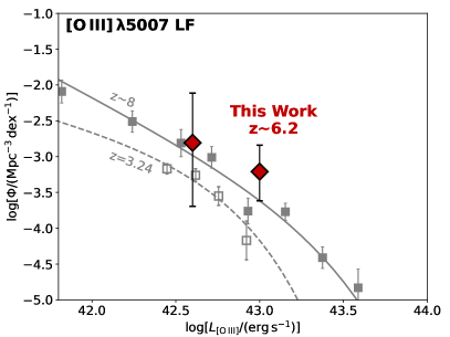
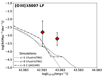
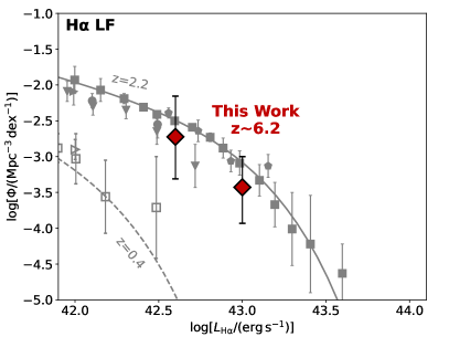
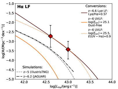
Figure 8: Top-left: $z\sim 6.2$ [O III] $\lambda$5007 line luminosity function derived in this work (red diamonds). For comparison we show the $z=3.24$ [O III] LF measured by Khostovan et al. (2015) through narrow-band imaging (open squares and dashed line), and $z\sim 8$ [O III] LF (De Barros et al., 2019) inferred from the UVLF and Spitzer/IRAC colors (filled squares and solid line). Top-right: Observed [O III] $\lambda$5007 luminosity function compared with those in simulations, including IllustrisTNG at $z=5$ (dashed gray line), $z=8$ (solid gray line; Shen et al. 2020) and the JAGUAR mock catalog at $z\sim 6.2$ (dash-dotted black line; Williams et al. 2018). Bottom-left: $z\sim 6.2$ H$\alpha$ line luminosity function derived in this work (red diamonds). For comparison, we show the H$\alpha$ LF measurements at $z=2.2$ (Geach et al. 2008, Hayes et al. 2010a, Tadaki et al. 2011, Lee et al. 2012, Sobral et al. 2013) and $z=0.4$ (Ly et al. 2007, Sobral et al. 2013). Best-fit Schechter functions at $z=2.2$ and 0.4 (Sobral et al., 2013) are shown in solid and dashed gray lines, respectively. Bottom-right: observed H$\alpha$ LF compared with those in simulations (IllustrisTNG at $z\sim 5$, dashed gray lines, Shen et al. 2020; JAGUAR mock catalog at $z\sim 6.2$, dash-dotted black line, Williams et al. 2018). We also compare with the $z\sim 6$ UVLF (Bouwens et al., 2021) by converting UV luminosity to H$\alpha$ luminosity under a constant SFR assumption (Kennicutt & Evans 2012; effectively $\log[\xi_{\mathrm{ion}}/(\mathrm{erg}^{-1}\mathrm{Hz})]=25.1$ and no dust attenuation) as shown in solid orange line. We also perform the conversion assuming an enhanced $\log[\xi_{\mathrm{ion}}/(\mathrm{erg}^{-1}\mathrm{Hz})]=25.5$ and $\mathrm{UV}-\mbox{H$\alpha$}$ color excess of 0.9 as shown in dotted orange line. Conversion from $z\sim 6.6$ Ly$\alpha$ LF (Konno et al. 2018; assuming a line ratio of Ly$\alpha$/H$\alpha$ $=$ 0.57) is shown in solid brown line.

5.2 [O III] $\lambda$5007 Luminosity Function

The [O III] $\lambda$5007 LF at $z\sim 6.2$ is shown in the top-left panel of Figure 8. For comparison, we also plot the [O III] $\lambda$5007 LF measured by Khostovan et al. (2015) at $z=3.24$, the highest-redshift [O III] LF measurement that is accessible from the ground using the rest-frame H₂ 1–0 S(1) narrow-band filter in the $K$ band (2.12 $\mathrm{\SIUnitSymbolMicro m}$). We also compare our results with the $z\sim 8$ [O III] LF derived by De Barros et al. (2019) based on the UV LF and the relation between UV and [O III]+H$\beta$ luminosities as inferred from Spitzer/IRAC [3.6]–[4.5] colors. For a fair comparison, we assumed that the [O III] $\lambda$5007 line contributes to $\sim 64$% of the total fluxes from H$\beta$+[O III] lines in the LFs of Khostovan et al. (2015) and De Barros et al. (2019). The adopted value is consistent with the median fraction observed with our sample, which is computed as $f_{\mathrm{[O\,III]\,5007}}/(1.33\,f_{\mathrm{[O\,III]\,5007}}+f_{\mathrm{H\alpha}}/2.86)$, assuming the theoretical ratio of 1/3 for [O III] 4959/5007 lines and 2.86 for H$\alpha$/H$\beta$ lines.

We find that our [O III] LF measurement at $z\sim 6.2$ is higher than the $z=3.24$ one (Khostovan et al., 2015) by a factor of $\sim 5$, and the scenario of constant [O III] LF can be ruled out from $\chi^{2}$ statistics ($p$-value $<0.05$). This indicates a strong evolution of [O III] line strength and therefore possibly of ionization parameter towards higher redshift. Our [O III] LF measurement is also higher than the $z\sim 8$ estimate in De Barros et al. (2019) by a factor of $\sim 2$. From $\chi^{2}$ statistics, these [O III] LF determinations at $z\sim 6.2$ and $\sim$8 may be consistent with each other ($p$-value $=0.3$; see also Matthee et al. 2022a for most recent results).

As shown in the top-right panel of Figure 8, we also compare our [O III] LF with those predicted by the IllustrisTNG simulation at $z=5$ and 8 (Shen et al., 2020) and the JAGUAR mock catalog (Williams et al., 2018). These simulations/realizations generally underpredict the observed [O III] $\lambda$5007 LF by a factor of $\sim$10. Because our $\Phi_{\mathrm{corr}}(L)$ measurement of the [O III] LF in the bright bin ($10^{42.8}-10^{43.2}$ $\mathrm{e}\mathrm{r}\mathrm{g}\,\mathrm{s}^{-1}$) is based on three sources (instead of only one) and the completeness correction factor is only $\sim 1.4$, we conclude that such a large excess of the [O III] LF compared to those in the simulation is real (see also recent simulations presented by Wilkins et al. 2023). These simulations are typically tuned to match empirical distributions where possible, which in the case of ionization parameter ($\log{U}$), are best characterized at low redshifts (e.g. the $\log{U}-Z/Z_{\mathrm{\odot}}$ relation from Carton et al. 2017, in the case of the JAGUAR mock catalog). This is now known to underpredict rest-frame optical line fluxes such as H$\alpha$ and [O III] at high redshifts (e.g., De Barros et al., 2019; Maseda et al., 2019) as we find here, indicating the likely strong evolution that will be revealed by larger samples in upcoming JWST surveys.

5.3 H$\alpha$ Luminosity Function

In the lower-left panel of Figure 8, we first compare our $z\sim 6.2$ H$\alpha$ LF measurement (uncorrected for dust attenuation) with those at $z\sim 0.4$ (Ly et al. 2007, Sobral et al. 2013; through 921 nm narrow band) and $z\sim 2.2$ (Geach et al. 2008, Hayes et al. 2010a, Tadaki et al. 2011, Lee et al. 2012, Sobral et al. 2013), which are still accessible from the ground using the 2.12 $\mathrm{\SIUnitSymbolMicro m}$ narrow-band filter. No direct measurement of H$\alpha$ LF exists beyond $z\sim 2.2$ before the launch of JWST. We find that the $z\sim 6.2$ H$\alpha$ LF measured with this work is higher than those at $z\sim 0.4$ but only slightly lower than those at $z\sim 2.2$, potentially suggesting weak or no evolution of H$\alpha$ LF ($p$-value $=0.36$ from $\chi^{2}$ statistics) from the end of EoR to the peak of cosmic star-formation history ($z\sim 2$, see Madau & Dickinson 2014 for a review). In the context of decreasing cosmic SFR density from $z\sim 2$ to 6, the observed constancy of the H$\alpha$ LFs between these two epochs possibly indicates, (i) a higher ionizing photon production efficiency at higher redshift (see discussion in Section 4.5 and reference therein), which leads to a higher $L_{\mathrm{H\alpha}}/\mathrm{SFR}$ ratio in the EoR, and (ii) a decreasing obscured fraction of H$\alpha$ emission, and therefore decreasing obscured fraction of cosmic SFR density from $z\sim 2$ to 6 as shown in recent ALMA dust-continuum source surveys (e.g., Bouwens et al., 2020; Casey et al., 2021; Zavala et al., 2021; Sun et al., 2022b).

In the lower-right panel of Figure 8, we show that our $z\sim 6.2$ H$\alpha$ LF measurement is 6–8 times higher than those predicted in the IllustrisTNG simulation ($z\sim 5$; Shen et al. 2020) and JAGUAR mock catalog ($z\sim 6.2$; Williams et al. 2018), similar to the [O III] LF. As discussed in Section 5.2, this reflects our limited understanding of rest-frame optical emission line strength of $z\gtrsim 6$ galaxies before the launch of JWST. This is likely caused by the underestimate of ionizing luminosities for $z\gtrsim 6$ galaxies with sub-solar metallicities (Williams et al., 2018) like those in our sample.

In addition to this, if we simply translate the $z\sim 6$ UV LF (e.g., Bouwens et al. 2021) to H$\alpha$ LF assuming the constant SFR conversions in Kennicutt & Evans (2012), the volume density of H$\alpha$ emitters would be underpredicted by $\sim 100$ times at $L_{\mathrm{H\alpha}}>10^{42.6}$ $\mathrm{e}\mathrm{r}\mathrm{g}\,\mathrm{s}^{-1}$. This suggests that, (i) the dust attenuation is still substantial for UV-luminous galaxies even at $z>6$ as is shown in recent ALMA studies (e.g., Schouws et al., 2022; Algera et al., 2023; Inami et al., 2022), despite a decreasing volume density of obscured SFR, and (ii) an enhanced $\xi_{\mathrm{ion}}$ at high redshift when compared with the local Universe. If we assume a typical $\log[\xi_{\mathrm{ion}}/(\mathrm{erg}^{-1}\,\mathrm{Hz})]=25.5$ for galaxies at $z\sim 6$ (see Section 4.6), the observed H$\alpha$ LF can be well matched to the conversion from the UV LF with a color excess of $E(\mathrm{UV}-\mathrm{H\alpha})=0.9\pm 0.5$. This can be translated to an $E(B-V)=0.33\pm 0.18$ and $A_{V}=1.3\pm 0.7$ assuming Calzetti et al. (2000) extinction law, and also $E(B-V)=0.11\pm 0.06$ and $A_{V}=0.30\pm 0.17$ assuming the SMC extinction law of Gordon et al. (2003), both adopting the canonical $E(B-V)$ ratio of 0.44 between stellar continuum and nebular lines (Calzetti et al., 2000).

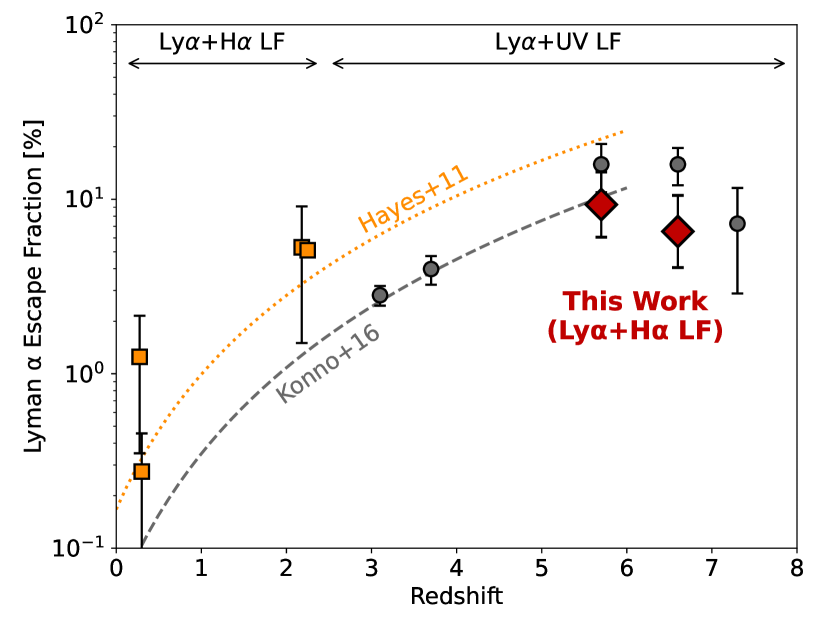
Figure 9: Global escape fraction of Ly$\alpha$ photons versus redshift. Ly$\alpha$ escape fraction at $z=5.7$ and 6.6 based on Ly$\alpha$ LF in Konno et al. (2018) and H$\alpha$ LF measured in this work are shown as red diamonds (see Section 5.3). $z\simeq 0.2-2.2$ measurements using Ly$\alpha$ and H$\alpha$ LFs are shown in orange squares (Deharveng et al., 2008; Cowie et al., 2010; Hayes et al., 2010b, 2011; Sobral et al., 2017), and the best-fit relation for the $z\simeq 0-6$ compilations in Hayes et al. (2011) is shown as the dotted orange line. $z\simeq 3-8$ measurements using Ly$\alpha$ and UV LFs compiled by Konno et al. (2016) are shown in gray circles, and the best-fit relation for their $z\simeq 0-6$ compilation is shown as the dashed gray line.

5.4 Implication for the Global Ly$\alpha$ Escape Fraction

As shown in the lower-right panel of Figure 8, our observed H$\alpha$ LF can match the observed Ly$\alpha$ LF at $z=6.6$ (Konno et al., 2018) assuming a Ly$\alpha$/H$\alpha$ flux ratio of $0.57_{-0.22}^{+0.35}$. We note that this also assumes that both Ly$\alpha$ and H$\alpha$ emission is from the same population of star-forming galaxies. The best match to the Ly$\alpha$ LF at $z=5.7$ (also Konno et al., 2018) would indicate a Ly$\alpha$/H$\alpha$ flux ratio of $0.81_{-0.28}^{+0.44}$. Considering a theoretical Ly$\alpha$/H$\alpha$ flux ratio of 8.7 from Case B recombination (see Hayes et al. 2011 and Henry et al. 2015) and assuming no evolution of H$\alpha$ LF from $z=5.7$ to 6.6, this suggests a global Ly$\alpha$ escape fraction ($f_{\mathrm{Ly\alpha}}^{\mathrm{esc}}=f(\mathrm{Ly\alpha})/f(\mathrm{H\alpha})/8.7$) of $6.5_{-2.4}^{+4.0}$% at $z\sim 6.6$ and $9.3_{-3.2}^{+5.0}$% at $z\sim 5.7$. This is consistent with recent JWST measurements of $f_{\mathrm{Ly\alpha}}^{\mathrm{esc}}$ based on Ly$\alpha$-selected galaxies at $z\sim 6$ (Ning et al., 2023). Note that these values are computed from the observed H$\alpha$ LF, and the intrinsic H$\alpha$ LF at $z\sim 6.2$ could be even higher because of the dust extinction correction, which may lead to a potential overestimate of $f_{\mathrm{Ly\alpha}}^{\mathrm{esc}}$.

As shown in Figure 9, both values of $f_{\mathrm{Ly\alpha}}^{\mathrm{esc}}$ are consistent with the global Ly$\alpha$ escape fraction found at $z\sim 2.2$ through the direct comparison of Ly$\alpha$/H$\alpha$ LFs (e.g., Hayes et al., 2010b; Sobral et al., 2017), but only $\sim 1/4$ of the early measurement of $f_{\mathrm{Ly\alpha}}^{\mathrm{esc}}$ at $z\sim 6$ in Hayes et al. (2011, $\sim 30$%) and $\sim 1/2$ of that in Konno et al. (2016, $\sim 15$%). As discussed in Konno et al. (2016), the difference in measured $f_{\mathrm{Ly\alpha}}^{\mathrm{esc}}$ between Hayes et al. (2011) and Konno et al. (2016) is mainly from the different lower limits of Ly$\alpha$ and UV luminosities for the integration of their densities. In previous literature, the estimate of Ly$\alpha$ escape fraction at $z>2.2$ relied on the conversion between UV and H$\alpha$ SFR because direct H$\alpha$ luminosity measurement was impossible from the ground. However, the H$\alpha$ luminosity could be underestimated from SFR with the classical Kennicutt & Evans (2012) conversion because of an enhanced $\xi_{\mathrm{ion}}$ at higher redshift, leading to an overestimated Ly$\alpha$ escape fraction (see also Matthee et al. 2022b, Naidu et al. 2022).

Our measurement further suggests no or weak evolution of Ly$\alpha$ escape fraction at $z\simeq 2-6$, in contrast to previous estimates that generally predict a $f_{\mathrm{Ly\alpha}}^{\mathrm{esc}}\propto(1+z)^{2.6}\sim(1+z)^{2.8}$ evolution (see Hayes et al. 2011, Konno et al. 2016 and a review by Ouchi et al. 2020). Despite this, the general picture of declining $f_{\mathrm{Ly\alpha}}^{\mathrm{esc}}$ at $z>6$ when compared with those at $z=3.1$ and 5.7 (e.g., Konno et al., 2016, 2018) would still remain valid, which is consistent with the increasing neutral fraction of intergalactic medium at higher redshifts. A more solid assessment would come in the future by obtaining Ly$\alpha$ spectroscopy of the same targets, which could provide direct information on Ly$\alpha$/H$\alpha$ line ratio.

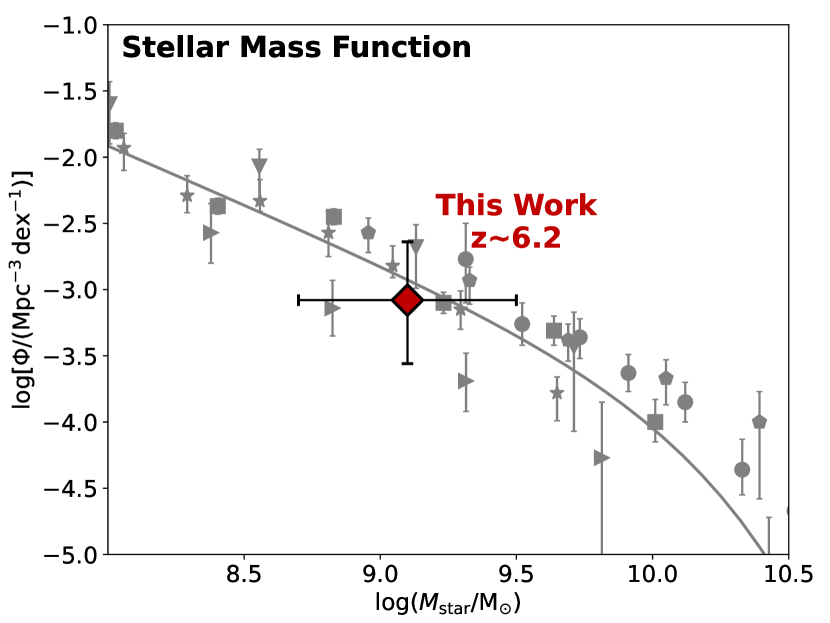
Figure 10: Comparison with galaxy stellar mass function at $z\sim 6$ (Duncan et al. 2014, pentagons; Grazian et al. 2015, circles; Song et al. 2016, rightward triangles; Bhatawdekar et al. 2019, downward triangles; Kikuchihara et al. 2020, stars; Stefanon et al. 2021, squares). Compared with the best-fit Schechter function in Stefanon et al. (2022) as shown in the solid gray line, our sample recovers $88_{-57}^{+164}$% of $z\sim 6$ galaxies with stellar mass above $5\times 10^{8}\,$$\mathrm{M}_{\odot}$.

5.5 Biases & Comparison with Stellar Mass Function

The selection of both [O III] $\lambda$5007 and H$\alpha$ emitters could potentially bias our sample toward the high-metallicity end of emission-line galaxies at $z>6$, because metal-poor galaxies could have a lower [O III]/H$\alpha$ flux ratio (e.g., Harikane et al., 2018) and therefore the [O III] line could be fainter than the detection limit. Meanwhile, the requirement of H$\alpha$ detection can also bias our sample toward sources with higher instantaneous SFR and therefore younger stellar population, and sources with high [O III] luminosities (higher ionization parameters) but low H$\alpha$ luminosities can be potentially missed. In addition, the detection of line emitters requires the detection in direct imaging data, i.e., brighter than $\sim$25 AB mag in either the F322W2 or F444W band. This means that for a source with comparable line fluxes, such as those in our sample, it would not make the selection if the stellar mass was $\sim 0.5$ dex lower, leading to a selection bias against sources with large EWs (e.g., Maseda et al., 2018).

Bearing all of these potential biases in mind, we compare the volume densities of galaxies in our sample (using $1/V_{\mathrm{max}}$ method as in Section 5.1) with those of $z\sim 6$ galaxies with the similar stellar masses in Figure 10. The published samples include measurements from Duncan et al. (2014), Grazian et al. (2015), Song et al. (2016), Bhatawdekar et al. (2019), Kikuchihara et al. (2020) and Stefanon et al. (2021), and all their stellar masses have been converted to those with Chabrier (2003) IMF. With a mean stellar mass of $1.4_{-0.5}^{+0.7}\times 10^{9}$ $\mathrm{M}_{\odot}$, the total volume density of galaxies in our sample is $10^{-3.1\pm 0.5}$ $\mathrm{M}\mathrm{p}\mathrm{c}^{-3}\,\mathrm{d}\mathrm{e}\mathrm{x}^{-1}$. Such a volume density is derived assuming a stellar-mass bin from $4\times 10^{8}\sim 4\times 10^{9}$ $\mathrm{M}_{\odot}$. We also consider the error of stellar-mass measurements and small number statistics through MC simulation (similar to Section 5.1).

The volume density of emission-line galaxies in our sample is $0.7_{-0.5}^{+1.2}$ times the volume density of $z\sim 6$ galaxies with comparable stellar masses as measured in Stefanon et al. (2021) using their best-fit Schechter function. By integrating the stellar-mass function in Stefanon et al. (2021), we find that our sample recovers $66_{-44}^{+128}$% of the $z\simeq 6.0-6.6$ galaxies in the effective survey volume with stellar masses greater than $5\times 10^{8}$ $\mathrm{M}_{\odot}$. Such a high fraction of recovery suggests that our sample well represents a reasonably large subsample of $z\sim 6$ galaxies with $M_{\mathrm{star}}$ $\sim 10^{9}$ $\mathrm{M}_{\odot}$, and the emission-line galaxies are ubiquitous within such stellar mass and redshift ranges.

6 Summary

We present a sample of four H$\alpha$+[O III] $\lambda$5007 line emitters at $z=6.11-6.35$ discovered through JWST/NIRCam wide-field slitless spectroscopic observations obtained during the commissioning phase. Located in the field of the flux calibrator P330-E, all four galaxies in our sample were spectroscopically confirmed with robust detections of H$\alpha$ ($>3\sigma$) and [O III] $\lambda$5007 lines ($>5\sigma$), including the one at $z=6.11$ that has already been reported in Sun et al. (2022a, Paper I). [O II] $\lambda$3727 and [O III] $\lambda$4959 lines were also tentatively identified for a few sources. With the spectroscopic and photometric measurements obtained with JWST/NIRCam, we performed SED modeling, and analyzed their physical properties and volume densities. The main results are the following:

1. The median H$\beta$$+$[O III] line EW of galaxies in our sample is $416\pm 66$ Å, consistent with those inferred previously at $z\simeq 6.7-7.0$ from Spitzer/IRAC SED analysis (e.g., Endsley et al., 2021a, b). The median H$\alpha$ line EW is $239\pm 45$ Å, smaller than those inferred previously at $z\simeq 5.1-5.4$ in Rasappu et al. (2016, also from IRAC SED analysis). All [O III] and H$\alpha$ EWs of these $z>6$ galaxies are much larger than those in the local Universe with similar stellar masses.

2. Sources in our sample likely occupy the same parameter space as that of $z\sim 2$ star-forming galaxies in the [O III]/H$\beta$-[N II]/H$\alpha$ BPT diagram, but are located above the star-forming sequence of local galaxies in the diagram. This could be explained by their elevated N/O abundance at a given O/H ratio, and/or higher ionization parameters, like those seen with $z\sim 2$ galaxies.

3. Through the strong-line ratios, we show that these $z>6$ galaxies have been enriched to moderate metallicities ($\sim 0.4$ $\mathrm{Z}_{\odot}$), comparable to those of galaxies at $z=2-3$ with similar stellar masses. Combined with the direct metallicity measurements of low-mass galaxies obtained from the JWST/NIRSpec ERO data, we find a steep slope of the mass-metallicity relation in the EoR. This may indicate a rapid metallicity enrichment history in certain massive ($M_{\mathrm{star}}\gtrsim 10^{9}$ $\mathrm{M}_{\odot}$) galaxies at $z>6$.

4. The median H$\alpha$ EW of galaxies in our sample is higher than that of star-forming galaxies at $z\lesssim 2$, but is consistent with that at $z\simeq 4-5$ inferred previously. This may indicate a flattening of the redshift evolution of H$\alpha$ EWs towards the EoR.

5. The galaxies in our sample have a median ionizing photon production efficiency of $\log[\xi_{\mathrm{ion}}/(\mathrm{erg}^{-1}\,\mathrm{Hz})]=25.4\pm 0.2$. Even with some uncertainty associated with dust attenuation correction, this value appears consistent with the redshift evolution trend in previous studies where $d\log(\xi_{\mathrm{ion}})/dz=0.10\pm 0.02$. A higher $\xi_{\mathrm{ion}}$ at higher redshift can lead to a higher H$\alpha$-based SFR estimate when compared to that derived from UV, if the canonical conversion factors are used (e.g., Kennicutt & Evans, 2012).

6. We derived the [O III] $\lambda$5007 and H$\alpha$ line luminosity functions using the $1/V_{\mathrm{max}}$ method. This is the first time that these two line LFs can be directly measured in the EoR. The $z\sim 6.2$ [O III] LF we measured is higher than those measured previously at $z=3.24$ (Khostovan et al., 2015), but likely consistent with that inferred at $z\sim 8$ (De Barros et al., 2019). It is also higher than those in the IllustrisTNG simulation (Shen et al., 2020) and JAGUAR mock catalog (Williams et al., 2018) at comparable redshift by $\sim 10$ times.

7. Our measurements suggest weak or no evolution with the H$\alpha$ line LF from $z\sim 2$ to 6. The measured H$\alpha$ LF at $z\sim 6$ exceeds the predictions from certain previous simulations/realizations by a factor of 6–8. A simple conversion from the $z\sim 6$ UV LF assuming SFR(H$\alpha$) $=$ SFR(UV) would underpredict H$\alpha$ LF (at $L_{\mathrm{H\alpha}}>10^{42.6}$ $\mathrm{e}\mathrm{r}\mathrm{g}\,\mathrm{s}\,^{-1}$) by a factor of $\sim 100$. This suggests an enhanced ionizing photon production efficiency and a substantial dust attenuation for UV-luminous galaxies at $z\sim 6$.

8. By directly comparing the Ly$\alpha$ and H$\alpha$ LF at $z\sim 6$, we find a global Ly$\alpha$ escape fraction of $9.3_{-3.2}^{+5.0}$% at $z=5.7$ and $6.5_{-2.4}^{+4.0}$% at $z=6.6$. In contrast to previous studies that used UV-based SFR to infer H$\alpha$ and therefore intrinsic Ly$\alpha$ luminosity, our study suggests no or weak evolution of the Ly$\alpha$ escape fraction at $z\simeq 2-6$. Despite this, the general picture of declining $f_{\mathrm{Ly\alpha}}^{\mathrm{esc}}$ at $z>6$ should still remain valid.

9. Despite some potential biases inherent in our selection of [O III]$+$H$\alpha$ emitters, the four galaxies in our sample have already contributed to a volume density of $10^{-3.1\pm 0.5}$ $\mathrm{M}\mathrm{p}\mathrm{c}^{-3}\,\mathrm{d}\mathrm{e}\mathrm{x}^{-1}$. This means that our sample recovers $66_{-44}^{+128}$% of the $z=6.0-6.6$ galaxies within the effective survey volume with $M_{\mathrm{star}}>5\times 10^{8}$ $\mathrm{M}_{\odot}$. Such a high recovery fraction indicates a low selection bias of our sample as well as the ubiquity of emission-line galaxies within such stellar-mass and redshift ranges.

Appendix A Completeness and Effective Survey Volume

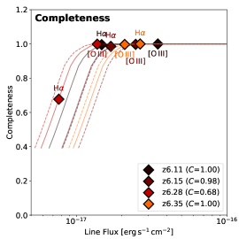
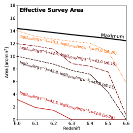
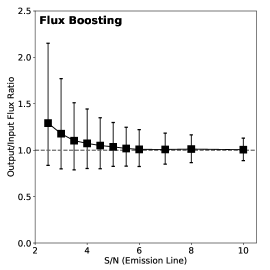
Figure A1: Left: Completeness of line emission detection. For each source at $z=6.11-6.35$, we show the simulated completeness as a function of input line flux according to the depth of their observation setup. Completeness functions for H$\alpha$ and [O III] lines are shown as solid and dashed curves, respectively. The synthesized completeness of line detections for each source is shown in the figure legend. Middle: Effective survey area as a function of redshift. The maximum survey area is shown as the solid black line, and effective survey area for four sources in our sample are shown as colored curves computed from the measured line luminosities. Right: Flux boosting effect (output/input line flux ratio) as a function of input line S/N modeled in our Monte Carlo simulation. The error bars represent 16th and 84th percentiles of the output flux ratios for each realization.

A.1 Completeness

To compute the completeness of all [O III] $\lambda$5007 and H$\alpha$ line detections, we first select faint continuum sources (F444W $>24$ AB mag) for which the grism observations yielded similar spectral coverages as those of $z>6$ line emitters. These continuum sources were observed with the same numbers of integrations with each module/grism combination (AR, BR, AC and BC) at the wavelength of interest (i.e., [O III] $\lambda$5007 and H$\alpha$ wavelengths at $z\sim 6.2$) as those of each line emitter, respectively. However, these F444W sources have no continuum or line emission detected in the grism data.

We then extract and coadd their 2D spectral image, and inject mock line emissions randomly at the same wavelength range of [O III] $\lambda$5007 and H$\alpha$ lines at $z=5.9-6.4$. No mock line emissions are injected at $z>6.4$ [O III]/H$\alpha$ wavelengths. This is because the observed H$\alpha$ wavelengths at these redshifts are too close to the red end of the F444W filter, and therefore the number of coadded integrations can decrease significantly in the 2D spectral images of these faint continuum sources, resulting in jumps of RMS noise. The injected line emissions are represented as 2D Gaussian profiles with FWHM $=5\sim 6$ pixel in both directions, similar to those of the sources in our sample. The line fluxes and errors are measured using the same method as we applied for the real line detections. The injected line emissions are at various strengths that yield detections at significance levels, ranging from $2\sigma$–$100\sigma$.

Based on the median output line flux errors, we are able to derive the fraction of $\geq 3\sigma$ detections for each of the [O III]/H$\alpha$ line fluxes in our sample, which is the completeness of each line detection. In reality, we find that the fraction of $\geq 3\sigma$ detections is well correlated with the S/N of input line, which is defined as the input line flux divided by the median output line flux error. For injected line emissions with input S/N of 5, the completeness of $3\sigma$ detection is 97%. However, this decreases to 58% for injected emission lines with a input S/N of 3. Such a completeness function of input line S/N is used to compute the completeness of line detections in our sample. The left panel of Figure A1 shows the completeness of all line detections as a function of the line fluxes. Except for the H$\alpha$ line of P330E-z6.28 that has a completeness of $\sim$60%, the completeness of all of the other lines are close to 100%. The synthesized completeness is computed as the product of [O III] and H$\alpha$ line completeness, which is given in the lower-right corner of the same panel.

A.2 Survey Volume

The maximum survey volume of each source in our sample is computed from the RMS map of F322W2 and F444W grism images. We first measure the RMS noise (unit: DN/s) of individual grism integrations taken with each of the four module/grism combinations in both F322W2 and F444W band, respectively. We then constructed the mosaicked RMS maps for grism images based on the measured noises and the pointing information of the telescope. We are then able to convert these to the maps of $3\sigma$ detection threshold for [O III] and H$\alpha$ line luminosities at $z=6.0\sim 6.6$ using (i) the sensitivity curves of four module/grism combinations in F322W2/F444W filter, and (ii) the relation between the RMS noise of 2D spectral image and the median line flux error obtained from the simulations described above. For each source in our sample, we compute the overlapping area from $z=6.0$ to $z=6.6$ at a step of $\Delta z=0.1$, where both their [O III] and H$\alpha$ line luminosities are above the detection threshold.

The maximum survey areas for all four sources in our sample as functions of redshift are shown in the middle panel of Figure A1. With the lowest H$\alpha$ and [O III] luminosities, source P330E-z6.28 can only be detected in the deepest 1–2 $\mathrm{a}\mathrm{r}\mathrm{c}\mathrm{m}\mathrm{i}\mathrm{n}^{2}$ area of the survey that contains the flux calibrator, consistent with what we observed. The maximum survey volume is then integrated from the maximum survey area across $z=6.0-6.6$. We also run MC simulations to quantify the errors of maximum survey volume propagated from the uncertainty of line flux, which is small ($\sim$ 5%) for luminous emitters like P330E-z6.35 but large ($\sim$100%) for faint emitters like P330E-z6.28. We also consider the reduction of maximum survey volume caused by the existence of bright continuum sources in the field. We conclude that the bright continuum contamination will only result in a small reduction ($\lesssim 5$%) of maximum survey volume from visual inspection of the extracted spectra of faint continuum sources (F444W $\gtrsim 24$ AB mag). This is because both R and C grism data are available and the field is sparse of bright stars (galactic latitude $b=+42$°). Such a small reduction is not worthy of correction when compared with the large uncertainty from small number statistics.

A.3 Flux Boosting and Eddington Bias

The flux measurements of low-significance emission lines often suffer from the flux-boosting effect because the Gaussian line-profile fitting routine always searches for the peak of the signal and returns a positive flux. If uncorrected, this will result in an overestimate of the volume density of luminous sources, also known as the Eddington bias (Eddington, 1913). The flux-boosting effect is quantified by comparing the injected and output line fluxes at input line S/N from 2 to 100 (Appendix A.1). For each input line S/N, we study the 16-50-84th percentiles of the output/input line flux ratios, which is shown as the right panel of Figure A1. Such a flux-boosting effect is corrected for our line luminosity and LF measurements, and the line luminosity could be boosted by 18% for a S/N $=$ 3 detection but only 5% at S/N $=$5. This is also the reason why 58% of lines with input S/N $=$ 3 are actually detected at S/N $\geq$ 3, instead of 50%, as described in the Appendix A.1.

References

- Abazajian et al. (2009) Abazajian, K. N., Adelman-McCarthy, J. K., Agüeros, M. A., et al. 2009, ApJS, 182, 543, doi: 10.1088/0067-0049/182/2/543
- Algera et al. (2023) Algera, H. S. B., Inami, H., Oesch, P. A., et al. 2023, MNRAS, 518, 6142, doi: 10.1093/mnras/stac3195
- Anders & Fritze-v. Alvensleben (2003) Anders, P., & Fritze-v. Alvensleben, U. 2003, A&A, 401, 1063, doi: 10.1051/0004-6361:20030151
- Arellano-Córdova et al. (2022) Arellano-Córdova, K. Z., Berg, D. A., Chisholm, J., et al. 2022, ApJ, 940, L23, doi: 10.3847/2041-8213/ac9ab2
- Astropy Collaboration et al. (2018) Astropy Collaboration, Price-Whelan, A. M., Sipőcz, B. M., et al. 2018, AJ, 156, 123, doi: 10.3847/1538-3881/aabc4f
- Atek et al. (2022) Atek, H., Furtak, L. J., Oesch, P., et al. 2022, MNRAS, 511, 4464, doi: 10.1093/mnras/stac360
- Baldwin et al. (1981) Baldwin, J. A., Phillips, M. M., & Terlevich, R. 1981, PASP, 93, 5, doi: 10.1086/130766
- Bertin & Arnouts (1996) Bertin, E., & Arnouts, S. 1996, A&AS, 117, 393, doi: 10.1051/aas:1996164
- Bhatawdekar et al. (2019) Bhatawdekar, R., Conselice, C. J., Margalef-Bentabol, B., & Duncan, K. 2019, MNRAS, 486, 3805, doi: 10.1093/mnras/stz866
- Bian et al. (2018) Bian, F., Kewley, L. J., & Dopita, M. A. 2018, ApJ, 859, 175, doi: 10.3847/1538-4357/aabd74
- Boquien et al. (2019) Boquien, M., Burgarella, D., Roehlly, Y., et al. 2019, A&A, 622, A103, doi: 10.1051/0004-6361/201834156
- Bouwens et al. (2020) Bouwens, R., González-López, J., Aravena, M., et al. 2020, ApJ, 902, 112, doi: 10.3847/1538-4357/abb830
- Bouwens et al. (2016a) Bouwens, R. J., Smit, R., Labbé, I., et al. 2016a, ApJ, 831, 176, doi: 10.3847/0004-637X/831/2/176
- Bouwens et al. (2016b) Bouwens, R. J., Oesch, P. A., Labbé, I., et al. 2016b, ApJ, 830, 67, doi: 10.3847/0004-637X/830/2/67
- Bouwens et al. (2021) Bouwens, R. J., Oesch, P. A., Stefanon, M., et al. 2021, AJ, 162, 47, doi: 10.3847/1538-3881/abf83e
- Boyer et al. (2022) Boyer, M. L., Anderson, J., Gennaro, M., et al. 2022, Research Notes of the American Astronomical Society, 6, 191, doi: 10.3847/2515-5172/ac923a
- Boyett et al. (2022) Boyett, K., Mascia, S., Pentericci, L., et al. 2022, ApJ, 940, L52, doi: 10.3847/2041-8213/ac9f17
- Bradley et al. (2020) Bradley, L., Sipőcz, B., Robitaille, T., et al. 2020, astropy/photutils: 1.0.0, 1.0.0, Zenodo, doi: 10.5281/zenodo.4044744
- Brinchmann (2022) Brinchmann, J. 2022, arXiv e-prints, arXiv:2208.07467. https://arxiv.org/abs/2208.07467
- Brinchmann et al. (2004) Brinchmann, J., Charlot, S., White, S. D. M., et al. 2004, MNRAS, 351, 1151, doi: 10.1111/j.1365-2966.2004.07881.x
- Bruzual & Charlot (2003) Bruzual, G., & Charlot, S. 2003, MNRAS, 344, 1000, doi: 10.1046/j.1365-8711.2003.06897.x
- Calzetti et al. (2000) Calzetti, D., Armus, L., Bohlin, R. C., et al. 2000, ApJ, 533, 682, doi: 10.1086/308692
- Cameron et al. (2023) Cameron, A. J., Saxena, A., Bunker, A. J., et al. 2023, arXiv e-prints, arXiv:2302.04298, doi: 10.48550/arXiv.2302.04298
- Carnall et al. (2023) Carnall, A. C., Begley, R., McLeod, D. J., et al. 2023, MNRAS, 518, L45, doi: 10.1093/mnrasl/slac136
- Carton et al. (2017) Carton, D., Brinchmann, J., Shirazi, M., et al. 2017, MNRAS, 468, 2140, doi: 10.1093/mnras/stx545
- Casey et al. (2021) Casey, C. M., Zavala, J. A., Manning, S. M., et al. 2021, ApJ, 923, 215, doi: 10.3847/1538-4357/ac2eb4
- Ceverino et al. (2021) Ceverino, D., Hirschmann, M., Klessen, R. S., et al. 2021, MNRAS, 504, 4472, doi: 10.1093/mnras/stab1206
- Chabrier (2003) Chabrier, G. 2003, PASP, 115, 763, doi: 10.1086/376392
- Charlot et al. (2002) Charlot, S., Kauffmann, G., Longhetti, M., et al. 2002, MNRAS, 330, 876, doi: 10.1046/j.1365-8711.2002.05157.x
- Cowie et al. (2010) Cowie, L. L., Barger, A. J., & Hu, E. M. 2010, ApJ, 711, 928, doi: 10.1088/0004-637X/711/2/928
- Curti et al. (2020) Curti, M., Mannucci, F., Cresci, G., & Maiolino, R. 2020, MNRAS, 491, 944, doi: 10.1093/mnras/stz2910
- Curti et al. (2022) Curti, M., Hayden-Pawson, C., Maiolino, R., et al. 2022, MNRAS, 512, 4136, doi: 10.1093/mnras/stac544
- Curti et al. (2023) Curti, M., D’Eugenio, F., Carniani, S., et al. 2023, MNRAS, 518, 425, doi: 10.1093/mnras/stac2737
- De Barros et al. (2019) De Barros, S., Oesch, P. A., Labbé, I., et al. 2019, MNRAS, 489, 2355, doi: 10.1093/mnras/stz940
- Deharveng et al. (2008) Deharveng, J.-M., Small, T., Barlow, T. A., et al. 2008, ApJ, 680, 1072, doi: 10.1086/587953
- Driver & Robotham (2010) Driver, S. P., & Robotham, A. S. G. 2010, MNRAS, 407, 2131, doi: 10.1111/j.1365-2966.2010.17028.x
- Duncan et al. (2014) Duncan, K., Conselice, C. J., Mortlock, A., et al. 2014, MNRAS, 444, 2960, doi: 10.1093/mnras/stu1622
- Eddington (1913) Eddington, A. S. 1913, MNRAS, 73, 359, doi: 10.1093/mnras/73.5.359
- Egami et al. (2005) Egami, E., Kneib, J. P., Rieke, G. H., et al. 2005, ApJ, 618, L5, doi: 10.1086/427550
- Emami et al. (2020) Emami, N., Siana, B., Alavi, A., et al. 2020, ApJ, 895, 116, doi: 10.3847/1538-4357/ab8f97
- Endsley et al. (2021a) Endsley, R., Stark, D. P., Charlot, S., et al. 2021a, MNRAS, 502, 6044, doi: 10.1093/mnras/stab432
- Endsley et al. (2021b) Endsley, R., Stark, D. P., Chevallard, J., & Charlot, S. 2021b, MNRAS, 500, 5229, doi: 10.1093/mnras/staa3370
- Erb et al. (2006) Erb, D. K., Steidel, C. C., Shapley, A. E., et al. 2006, ApJ, 647, 128, doi: 10.1086/505341
- Faisst et al. (2019) Faisst, A. L., Capak, P. L., Emami, N., Tacchella, S., & Larson, K. L. 2019, ApJ, 884, 133, doi: 10.3847/1538-4357/ab425b
- Faisst et al. (2016) Faisst, A. L., Capak, P., Hsieh, B. C., et al. 2016, ApJ, 821, 122, doi: 10.3847/0004-637X/821/2/122
- Fumagalli et al. (2012) Fumagalli, M., Patel, S. G., Franx, M., et al. 2012, ApJ, 757, L22, doi: 10.1088/2041-8205/757/2/L22
- Gaia Collaboration et al. (2018) Gaia Collaboration, Brown, A. G. A., Vallenari, A., et al. 2018, A&A, 616, A1, doi: 10.1051/0004-6361/201833051
- Gardner et al. (2023) Gardner, J. P., Mather, J. C., Abbott, R., et al. 2023, arXiv e-prints, arXiv:2304.04869, doi: 10.48550/arXiv.2304.04869
- Geach et al. (2008) Geach, J. E., Smail, I., Best, P. N., et al. 2008, MNRAS, 388, 1473, doi: 10.1111/j.1365-2966.2008.13481.x
- Gehrels (1986) Gehrels, N. 1986, ApJ, 303, 336, doi: 10.1086/164079
- Gordon et al. (2003) Gordon, K. D., Clayton, G. C., Misselt, K. A., Landolt, A. U., & Wolff, M. J. 2003, ApJ, 594, 279, doi: 10.1086/376774
- Gordon et al. (2022) Gordon, K. D., Bohlin, R., Sloan, G. C., et al. 2022, AJ, 163, 267, doi: 10.3847/1538-3881/ac66dc
- Grazian et al. (2015) Grazian, A., Fontana, A., Santini, P., et al. 2015, A&A, 575, A96, doi: 10.1051/0004-6361/201424750
- Greene et al. (2017) Greene, T. P., Kelly, D. M., Stansberry, J., et al. 2017, Journal of Astronomical Telescopes, Instruments, and Systems, 3, 035001, doi: 10.1117/1.JATIS.3.3.035001
- Harikane et al. (2018) Harikane, Y., Ouchi, M., Shibuya, T., et al. 2018, ApJ, 859, 84, doi: 10.3847/1538-4357/aabd80
- Hayes et al. (2010a) Hayes, M., Schaerer, D., & Östlin, G. 2010a, A&A, 509, L5, doi: 10.1051/0004-6361/200913217
- Hayes et al. (2011) Hayes, M., Schaerer, D., Östlin, G., et al. 2011, ApJ, 730, 8, doi: 10.1088/0004-637X/730/1/8
- Hayes et al. (2010b) Hayes, M., Östlin, G., Schaerer, D., et al. 2010b, Nature, 464, 562, doi: 10.1038/nature08881
- Helton et al. (2023) Helton, J. M., Sun, F., Woodrum, C., et al. 2023, arXiv e-prints, arXiv:2302.10217, doi: 10.48550/arXiv.2302.10217
- Henry et al. (2015) Henry, A., Scarlata, C., Martin, C. L., & Erb, D. 2015, ApJ, 809, 19, doi: 10.1088/0004-637X/809/1/19
- Horne (1986) Horne, K. 1986, PASP, 98, 609, doi: 10.1086/131801
- Inami et al. (2022) Inami, H., Algera, H. S. B., Schouws, S., et al. 2022, MNRAS, 515, 3126, doi: 10.1093/mnras/stac1779
- Jones et al. (2020) Jones, T., Sanders, R., Roberts-Borsani, G., et al. 2020, ApJ, 903, 150, doi: 10.3847/1538-4357/abb943
- Katz et al. (2023) Katz, H., Saxena, A., Cameron, A. J., et al. 2023, MNRAS, 518, 592, doi: 10.1093/mnras/stac2657
- Kauffmann et al. (2003a) Kauffmann, G., Heckman, T. M., Tremonti, C., et al. 2003a, MNRAS, 346, 1055, doi: 10.1111/j.1365-2966.2003.07154.x
- Kauffmann et al. (2003b) Kauffmann, G., Heckman, T. M., White, S. D. M., et al. 2003b, MNRAS, 341, 33, doi: 10.1046/j.1365-8711.2003.06291.x
- Kennicutt & Evans (2012) Kennicutt, R. C., & Evans, N. J. 2012, ARA&A, 50, 531, doi: 10.1146/annurev-astro-081811-125610
- Kewley et al. (2013) Kewley, L. J., Dopita, M. A., Leitherer, C., et al. 2013, ApJ, 774, 100, doi: 10.1088/0004-637X/774/2/100
- Kewley et al. (2001) Kewley, L. J., Dopita, M. A., Sutherland, R. S., Heisler, C. A., & Trevena, J. 2001, ApJ, 556, 121, doi: 10.1086/321545
- Khostovan et al. (2015) Khostovan, A. A., Sobral, D., Mobasher, B., et al. 2015, MNRAS, 452, 3948, doi: 10.1093/mnras/stv1474
- Kikuchihara et al. (2020) Kikuchihara, S., Ouchi, M., Ono, Y., et al. 2020, ApJ, 893, 60, doi: 10.3847/1538-4357/ab7dbe
- Kojima et al. (2017) Kojima, T., Ouchi, M., Nakajima, K., et al. 2017, PASJ, 69, 44, doi: 10.1093/pasj/psx017
- Konno et al. (2016) Konno, A., Ouchi, M., Nakajima, K., et al. 2016, ApJ, 823, 20, doi: 10.3847/0004-637X/823/1/20
- Konno et al. (2018) Konno, A., Ouchi, M., Shibuya, T., et al. 2018, PASJ, 70, S16, doi: 10.1093/pasj/psx131
- Kriek et al. (2015) Kriek, M., Shapley, A. E., Reddy, N. A., et al. 2015, ApJS, 218, 15, doi: 10.1088/0067-0049/218/2/15
- Labbé et al. (2013) Labbé, I., Oesch, P. A., Bouwens, R. J., et al. 2013, ApJ, 777, L19, doi: 10.1088/2041-8205/777/2/L19
- Lam et al. (2019) Lam, D., Bouwens, R. J., Labbé, I., et al. 2019, A&A, 627, A164, doi: 10.1051/0004-6361/201935227
- Lee et al. (2012) Lee, J. C., Ly, C., Spitler, L., et al. 2012, PASP, 124, 782, doi: 10.1086/666528
- Li et al. (2022) Li, M., Cai, Z., Bian, F., et al. 2022, arXiv e-prints, arXiv:2211.01382, doi: 10.48550/arXiv.2211.01382
- Ly et al. (2007) Ly, C., Malkan, M. A., Kashikawa, N., et al. 2007, ApJ, 657, 738, doi: 10.1086/510828
- Madau & Dickinson (2014) Madau, P., & Dickinson, M. 2014, ARA&A, 52, 415, doi: 10.1146/annurev-astro-081811-125615
- Maraston et al. (2013) Maraston, C., Pforr, J., Henriques, B. M., et al. 2013, MNRAS, 435, 2764, doi: 10.1093/mnras/stt1424
- Mármol-Queraltó et al. (2016) Mármol-Queraltó, E., McLure, R. J., Cullen, F., et al. 2016, MNRAS, 460, 3587, doi: 10.1093/mnras/stw1212
- Maseda et al. (2019) Maseda, M. V., Franx, M., Chevallard, J., & Curtis-Lake, E. 2019, MNRAS, 486, 3290, doi: 10.1093/mnras/stz818
- Maseda et al. (2018) Maseda, M. V., van der Wel, A., Rix, H.-W., et al. 2018, ApJ, 854, 29, doi: 10.3847/1538-4357/aaa76e
- Masters et al. (2014) Masters, D., McCarthy, P., Siana, B., et al. 2014, ApJ, 785, 153, doi: 10.1088/0004-637X/785/2/153
- Matthee et al. (2022a) Matthee, J., Mackenzie, R., Simcoe, R. A., et al. 2022a, arXiv e-prints, arXiv:2211.08255, doi: 10.48550/arXiv.2211.08255
- Matthee et al. (2017) Matthee, J., Sobral, D., Best, P., et al. 2017, MNRAS, 465, 3637, doi: 10.1093/mnras/stw2973
- Matthee et al. (2022b) Matthee, J., Naidu, R. P., Pezzulli, G., et al. 2022b, MNRAS, 512, 5960, doi: 10.1093/mnras/stac801
- Naidu et al. (2020) Naidu, R. P., Tacchella, S., Mason, C. A., et al. 2020, ApJ, 892, 109, doi: 10.3847/1538-4357/ab7cc9
- Naidu et al. (2022) Naidu, R. P., Matthee, J., Oesch, P. A., et al. 2022, MNRAS, 510, 4582, doi: 10.1093/mnras/stab3601
- Nakajima et al. (2016) Nakajima, K., Ellis, R. S., Iwata, I., et al. 2016, ApJ, 831, L9, doi: 10.3847/2041-8205/831/1/L9
- Nakajima et al. (2023) Nakajima, K., Ouchi, M., Isobe, Y., et al. 2023, arXiv e-prints, arXiv:2301.12825, doi: 10.48550/arXiv.2301.12825
- Nanayakkara et al. (2020) Nanayakkara, T., Brinchmann, J., Glazebrook, K., et al. 2020, ApJ, 889, 180, doi: 10.3847/1538-4357/ab65eb
- Ning et al. (2023) Ning, Y., Cai, Z., Jiang, L., et al. 2023, ApJ, 944, L1, doi: 10.3847/2041-8213/acb26b
- Oke & Gunn (1983) Oke, J. B., & Gunn, J. E. 1983, ApJ, 266, 713, doi: 10.1086/160817
- Osterbrock & Ferland (2006) Osterbrock, D. E., & Ferland, G. J. 2006, Astrophysics of gaseous nebulae and active galactic nuclei
- Ouchi et al. (2020) Ouchi, M., Ono, Y., & Shibuya, T. 2020, ARA&A, 58, 617, doi: 10.1146/annurev-astro-032620-021859
- Pontoppidan et al. (2022) Pontoppidan, K. M., Barrientes, J., Blome, C., et al. 2022, ApJ, 936, L14, doi: 10.3847/2041-8213/ac8a4e
- Rasappu et al. (2016) Rasappu, N., Smit, R., Labbé, I., et al. 2016, MNRAS, 461, 3886, doi: 10.1093/mnras/stw1484
- Reddy et al. (2015) Reddy, N. A., Kriek, M., Shapley, A. E., et al. 2015, ApJ, 806, 259, doi: 10.1088/0004-637X/806/2/259
- Reddy et al. (2018) Reddy, N. A., Shapley, A. E., Sanders, R. L., et al. 2018, ApJ, 869, 92, doi: 10.3847/1538-4357/aaed1e
- Rhoads et al. (2023) Rhoads, J. E., Wold, I. G. B., Harish, S., et al. 2023, ApJ, 942, L14, doi: 10.3847/2041-8213/acaaaf
- Rieke et al. (2023) Rieke, M. J., Kelly, D. M., Misselt, K., et al. 2023, PASP, 135, 028001, doi: 10.1088/1538-3873/acac53
- Rigby et al. (2023) Rigby, J., Perrin, M., McElwain, M., et al. 2023, PASP, 135, 048001, doi: 10.1088/1538-3873/acb293
- Roberts-Borsani et al. (2016) Roberts-Borsani, G. W., Bouwens, R. J., Oesch, P. A., et al. 2016, ApJ, 823, 143, doi: 10.3847/0004-637X/823/2/143
- Robertson (2022) Robertson, B. E. 2022, ARA&A, 60, 121, doi: 10.1146/annurev-astro-120221-044656
- Sanders et al. (2023a) Sanders, R. L., Shapley, A. E., Topping, M. W., Reddy, N. A., & Brammer, G. B. 2023a, arXiv e-prints, arXiv:2301.06696, doi: 10.48550/arXiv.2301.06696
- Sanders et al. (2023b) —. 2023b, arXiv e-prints, arXiv:2303.08149, doi: 10.48550/arXiv.2303.08149
- Sanders et al. (2021) Sanders, R. L., Shapley, A. E., Jones, T., et al. 2021, ApJ, 914, 19, doi: 10.3847/1538-4357/abf4c1
- Schaerer & de Barros (2009) Schaerer, D., & de Barros, S. 2009, A&A, 502, 423, doi: 10.1051/0004-6361/200911781
- Schaerer et al. (2022) Schaerer, D., Marques-Chaves, R., Barrufet, L., et al. 2022, A&A, 665, L4, doi: 10.1051/0004-6361/202244556
- Schechter (1976) Schechter, P. 1976, ApJ, 203, 297, doi: 10.1086/154079
- Schlawin et al. (2020) Schlawin, E., Leisenring, J., Misselt, K., et al. 2020, AJ, 160, 231, doi: 10.3847/1538-3881/abb811
- Schmidt (1968) Schmidt, M. 1968, ApJ, 151, 393, doi: 10.1086/149446
- Schouws et al. (2022) Schouws, S., Stefanon, M., Bouwens, R., et al. 2022, ApJ, 928, 31, doi: 10.3847/1538-4357/ac4605
- Shapley et al. (2015) Shapley, A. E., Reddy, N. A., Kriek, M., et al. 2015, ApJ, 801, 88, doi: 10.1088/0004-637X/801/2/88
- Shen et al. (2020) Shen, X., Vogelsberger, M., Nelson, D., et al. 2020, MNRAS, 495, 4747, doi: 10.1093/mnras/staa1423
- Shim et al. (2011) Shim, H., Chary, R.-R., Dickinson, M., et al. 2011, ApJ, 738, 69, doi: 10.1088/0004-637X/738/1/69
- Shivaei et al. (2018) Shivaei, I., Reddy, N. A., Siana, B., et al. 2018, ApJ, 855, 42, doi: 10.3847/1538-4357/aaad62
- Smit et al. (2016) Smit, R., Bouwens, R. J., Labbé, I., et al. 2016, ApJ, 833, 254, doi: 10.3847/1538-4357/833/2/254
- Smit et al. (2014) —. 2014, ApJ, 784, 58, doi: 10.1088/0004-637X/784/1/58
- Smit et al. (2015) Smit, R., Bouwens, R. J., Franx, M., et al. 2015, ApJ, 801, 122, doi: 10.1088/0004-637X/801/2/122
- Sobral et al. (2014) Sobral, D., Best, P. N., Smail, I., et al. 2014, MNRAS, 437, 3516, doi: 10.1093/mnras/stt2159
- Sobral et al. (2013) Sobral, D., Smail, I., Best, P. N., et al. 2013, MNRAS, 428, 1128, doi: 10.1093/mnras/sts096
- Sobral et al. (2017) Sobral, D., Matthee, J., Best, P., et al. 2017, MNRAS, 466, 1242, doi: 10.1093/mnras/stw3090
- Song et al. (2016) Song, M., Finkelstein, S. L., Ashby, M. L. N., et al. 2016, ApJ, 825, 5, doi: 10.3847/0004-637X/825/1/5
- Stark et al. (2013) Stark, D. P., Schenker, M. A., Ellis, R., et al. 2013, ApJ, 763, 129, doi: 10.1088/0004-637X/763/2/129
- Stark et al. (2015) Stark, D. P., Walth, G., Charlot, S., et al. 2015, MNRAS, 454, 1393, doi: 10.1093/mnras/stv1907
- Stark et al. (2017) Stark, D. P., Ellis, R. S., Charlot, S., et al. 2017, MNRAS, 464, 469, doi: 10.1093/mnras/stw2233
- Stefanon et al. (2022) Stefanon, M., Bouwens, R. J., Illingworth, G. D., et al. 2022, ApJ, 935, 94, doi: 10.3847/1538-4357/ac7e44
- Stefanon et al. (2021) Stefanon, M., Bouwens, R. J., Labbé, I., et al. 2021, ApJ, 922, 29, doi: 10.3847/1538-4357/ac1bb6
- Steidel et al. (2016) Steidel, C. C., Strom, A. L., Pettini, M., et al. 2016, ApJ, 826, 159, doi: 10.3847/0004-637X/826/2/159
- Steidel et al. (2014) Steidel, C. C., Rudie, G. C., Strom, A. L., et al. 2014, ApJ, 795, 165, doi: 10.1088/0004-637X/795/2/165
- Strom et al. (2017) Strom, A. L., Steidel, C. C., Rudie, G. C., et al. 2017, ApJ, 836, 164, doi: 10.3847/1538-4357/836/2/164
- Sun et al. (2022a) Sun, F., Egami, E., Pirzkal, N., et al. 2022a, ApJ, 936, L8, doi: 10.3847/2041-8213/ac8938
- Sun et al. (2022b) Sun, F., Egami, E., Fujimoto, S., et al. 2022b, ApJ, 932, 77, doi: 10.3847/1538-4357/ac6e3f
- Tacchella et al. (2018) Tacchella, S., Bose, S., Conroy, C., Eisenstein, D. J., & Johnson, B. D. 2018, ApJ, 868, 92, doi: 10.3847/1538-4357/aae8e0
- Tacchella et al. (2022) Tacchella, S., Johnson, B. D., Robertson, B. E., et al. 2022, arXiv e-prints, arXiv:2208.03281. https://arxiv.org/abs/2208.03281
- Tadaki et al. (2011) Tadaki, K.-I., Kodama, T., Koyama, Y., et al. 2011, PASJ, 63, 437, doi: 10.1093/pasj/63.sp2.S437
- Tamura et al. (2019) Tamura, Y., Mawatari, K., Hashimoto, T., et al. 2019, ApJ, 874, 27, doi: 10.3847/1538-4357/ab0374
- Tang et al. (2019) Tang, M., Stark, D. P., Chevallard, J., & Charlot, S. 2019, MNRAS, 489, 2572, doi: 10.1093/mnras/stz2236
- Tang et al. (2023) Tang, M., Stark, D. P., Chen, Z., et al. 2023, arXiv e-prints, arXiv:2301.07072, doi: 10.48550/arXiv.2301.07072
- Taylor et al. (2022) Taylor, A. J., Barger, A. J., & Cowie, L. L. 2022, ApJ, 939, L3, doi: 10.3847/2041-8213/ac959d
- Thomas et al. (2013) Thomas, D., Steele, O., Maraston, C., et al. 2013, MNRAS, 431, 1383, doi: 10.1093/mnras/stt261
- Topping et al. (2020a) Topping, M. W., Shapley, A. E., Reddy, N. A., et al. 2020a, MNRAS, 495, 4430, doi: 10.1093/mnras/staa1410
- Topping et al. (2020b) —. 2020b, MNRAS, 499, 1652, doi: 10.1093/mnras/staa2941
- Torrey et al. (2019) Torrey, P., Vogelsberger, M., Marinacci, F., et al. 2019, MNRAS, 484, 5587, doi: 10.1093/mnras/stz243
- Trump et al. (2023) Trump, J. R., Arrabal Haro, P., Simons, R. C., et al. 2023, ApJ, 945, 35, doi: 10.3847/1538-4357/acba8a
- Trussler et al. (2022) Trussler, J. A. A., Adams, N. J., Conselice, C. J., et al. 2022, arXiv e-prints, arXiv:2207.14265, doi: 10.48550/arXiv.2207.14265
- Wilkins et al. (2023) Wilkins, S. M., Lovell, C. C., Vijayan, A. P., et al. 2023, arXiv e-prints, arXiv:2301.13038, doi: 10.48550/arXiv.2301.13038
- Williams et al. (2018) Williams, C. C., Curtis-Lake, E., Hainline, K. N., et al. 2018, ApJS, 236, 33, doi: 10.3847/1538-4365/aabcbb
- Zavala et al. (2021) Zavala, J. A., Casey, C. M., Manning, S. M., et al. 2021, ApJ, 909, 165, doi: 10.3847/1538-4357/abdb27