Attacking the Spike: On the Transferability and Security of Spiking Neural Networks to Adversarial Examples

Abstract

Spiking neural networks (SNNs) have attracted much attention for their high energy efficiency and for recent advances in their classification performance. However, unlike traditional deep learning approaches, the analysis and study of the robustness of SNNs to adversarial examples remain relatively underdeveloped. In this work, we focus on advancing the adversarial attack side of SNNs and make three major contributions. First, we show that successful white-box adversarial attacks on SNNs are highly dependent on the underlying surrogate gradient technique, even in the case of adversarially trained SNNs. Second, using the best surrogate gradient technique, we analyze the transferability of adversarial attacks on SNNs and other state-of-the-art architectures like Vision Transformers (ViTs) and Big Transfer Convolutional Neural Networks (CNNs). We demonstrate that the adversarial examples created by non-SNN architectures are not misclassified often by SNNs. Third, due to the lack of an ubiquitous white-box attack that is effective across both the SNN and CNN/ViT domains, we develop a new white-box attack, the Auto Self-Attention Gradient Attack (Auto-SAGA). Our novel attack generates adversarial examples capable of fooling both SNN and non-SNN models simultaneously. Auto-SAGA is as much as $91.1\%$ more effective on SNN/ViT model ensembles and provides a $3\times$ boost in attack effectiveness on adversarially trained SNN ensembles compared to conventional white-box attacks like Auto-PGD. Our experiments and analyses are broad and rigorous covering three datasets (CIFAR-10, CIFAR-100 and ImageNet), five different white-box attacks and nineteen classifier models (seven for each CIFAR dataset and five models for ImageNet).

Introduction

There is an increasing demand to deploy machine intelligence to power-limited devices such as mobile electronics and Internet-of-Things (IoT), however, the computation complexity of deep learning models, coupled with energy consumption has become a challenge (Kugele et al. 2020; Shrestha et al. 2022). This motivates a new computing paradigm, bio-inspired energy efficient neuromorphic computing. As the underlying computational model, Spiking Neural Networks (SNNs) have drawn considerable interest (Davies et al. 2021). SNNs can provide high energy efficient solutions for resource-limited applications. For example, in (Tang et al. 2020) an SNN was used for a robot navigation task with Intel’s Loihi (Davies et al. 2018) and achieved a 276$\times$ reduction in energy as compared to a conventional machine learning approach. In (Rueckauer et al. 2022) it was reported that an SNN consumed 0.66$mJ$, 102 $mJ$ per sample on MNIST and CIFAR-10, while a Deep Neural Network (DNN) consumed 111 $mJ$ and 1035 $mJ$, resulting in 168$\times$ and 10$\times$ energy reduction, respectively. Emerging SNN techniques such as joint thresholding, leakage, and weight optimization using surrogate gradients have all led to improved performance. Both transfer based (Lu et al. 2020; Rathi et al. 2020, 2021) SNNs and backpropagation (BP) trained-from-scratch SNNs (Shrestha et al. 2018; Fang et al. 2020b, 2021a, 2021b) achieve similar performance to DNNs, while consuming considerably less energy.

On the other hand, the vulnerability of deep learning models to adversarial examples  (Goodfellow et al. 2014) is one of the main topics that has received much attention in recent research. An adversarial example is an input that has been manipulated with a small amount of noise such that a human being can correctly classify it. However, the adversarial example is misclassified by a machine learning model with high confidence. A large body of literature has been devoted to the development of both adversarial attacks (Tramer et al. 2020) and defenses (Zhang et al. 2020a) for CNNs.

As SNNs become more accurate and more widely adopted, their security vulnerabilities will emerge as an important issue. Recent work has been done to study some of the security aspects of the SNN (El-Allami et al. 2021; Sharmin et al. 2019, 2020; Goodfellow et al. 2015; Kundu et al. 2021; Liang et al. 2021), although not to the same extent as CNNs. To the best of our knowledge, there has not been rigorous analyses done on how the different choice of gradient estimations can effect white-box SNN attacks. In addition, it is an open question whether SNN adversarial examples are misclassified by other state-of-the-art models like Vision Transformers. Finally, there has not been any general attack method developed to break both SNNs and CNNs/ViTs simultaneously. Thus in our paper, we specifically focus on three key adversarial aspects:

1. How are white-box attacks on SNNs affected by different SNN surrogate gradient estimation techniques?

2. As SNNs have shown more robustness in previous studies (Sharmin et al. 2019; Liang et al. 2021), do adversarial examples generated by SNNs transfer to other models such as Vision Transformers and CNNs and vice versa?

3. Are there a white-box attacks that can effectively target both SNNs and CNNs/Vision Transformers, closing the transferability gap and achieving a high success rate?

These three questions are intrinsically linked: by first focusing on the surrogate gradient, we can develop effective SNN white-box attacks. These precise SNN attacks are the foundation for analyzing the transferability of adversarial examples between SNNs and other SOTA architectures (as posed in our second question). Based on the outcome of the second question (low attack transferability, which we show in Section SNN Transferability Study), we further develop a new attack capable of breaking SNN and non-SNN models simultaneously.

We organize the rest of our paper as follows: in Section SNN Models, we briefly introduce the different types of SNNs, whose security we analyze. In Section SNN Surrogate Gradient Estimation, we analyze the effect of seven different surrogate gradient estimators on white-box adversarial attacks. We show that the choice of surrogate gradient estimator is highly influential and must be carefully selected. In Section SNN Transferability Study, we use the best surrogate gradient estimator to study the transferability of adversarial examples generated by SNNs. Our transferability experiments demonstrate that traditional white-box attacks are not effective on both SNNs and other non-SNN models simultaneously, mandating the need for a new multi-model attack. In Section Transferability and Multi-Model Attacks, we develop a new multi-model attack capable of creating adversarial examples that are misclassified by both SNN and non-SNN models. Our attack is called the Auto Self-Attention Gradient Attack (Auto-SAGA) and we empirically show its superiority to MIM (Dong et al. 2018), PGD (Madry et al. 2018) and Auto-PGD (Croce et al. 2020).

Overall, we conduct rigorous analyses and experiments with 19 models across three datasets (CIFAR-10, CIFAR-100 and ImageNet) and four adversarial training methods. Our surrogate gradient and transferability results yield new insights into SNN security. Our newly proposed attack (Auto-SAGA) works on SNN/ViT/CNN ensembles with higher attack success rates (as much as $91.9\%$ improvement) and boosts the attack effectiveness on adversarially trained SNN ensembles by $3\times$ over conventional white-box attacks like Auto-PGD. All three of our major paper contributions significantly advance the security development of SNN adversarial machine learning.

SNN Models

In this section, we discuss the basics of the SNN architecture and of neural encoding. Widely used Leaky Integrate and Fire (LIF) neuron can be described by a system of difference equations as follows (Shrestha et al. 2022):

$$V[t]=\alpha V[t{-}1]+\sum_{i}w_{i}S_{i}[t]-\vartheta O[t-1]$$ (1a)

$$O[t]=u(V[t]-\vartheta)$$ (1b)

$$u(x)=0,x<0\text{ otherwise 1}$$ (1c)

where $V[t]$ denotes neuron’s membrane potential. $\alpha\in(0,1]$ is a time constant, which controls the decay speed of membrane potential. When $\alpha=1$, the model becomes Integrate and Fire (IF) neuron. $S_{i}[t]$ and $w_{i}$ are $i_{th}$ input and the associated weight. $\vartheta$ is the neuron’s threshold, $O[t]$ is the neuron’s output function, $u(\cdot)$ is the Heaviside step function. If $V[t]$ exceeds the threshold $\vartheta$, the neuron will fire a spike, hence $O[t]$ will be 1. Then, at the next time step, $V[t]$ will be decreased by $\vartheta$ in a procedure referred to as a reset (Shrestha et al. 2022).

Note that, in contrast to the continuous input domains of DNNs, in SNNs information is represented by discrete, binary spike trains. Therefore, data has to be mapped to spike domain for an SNN to process, this procedure is referred to as neural encoding, which plays an essential role in high performance SNN applications (Shrestha et al. 2022). A popular way to achieve such mapping is the direct encoding (Wu et al. 2019; Rathi et al. 2021). This method uses Current-Based neuron (CUBA) as the first layer in an SNN’s architecture. CUBA accepts continuous values instead of spikes (Fang et al. 2020a) such that a pixel value can be converted into a spike train and then directly fed to the SNN. Because direct encoding can reduce inference latency by a factor of $5{-}100$ (Rathi et al. 2021), recent works have achieved state-of-the-art results with this coding scheme (Rathi et al. 2021; Fang et al. 2021a; Kundu et al. 2021; Fang et al. 2020b), all experiments employ direct coding in this work.

SNN Training

Spiking neuron’s non-differentiable activation makes directly applying backpropagation (BP) difficult (Zhang et al. 2020b; Tavanaei et al. 2019). Training an SNN requires different approaches, which can be categorized as follows:

Conversion-based training. A common practice is to use spike numbers in a fixed time window (spike rate) to represent a numerical value. The input strength and neuron’s spike rate roughly have a linear relation (such behavior is similar to ReLU function in DNNs (Diehl et al. 2015)). Therefore, it is possible to pretrain a DNN model and map the weights to an SNN. However, simply mapping the weights suffers from performance degradation due to non-ideal input-spike rate linearity, over activation, and under activation (Rathi et al. 2021; Diehl et al. 2015). Additional post-processing and fine tuning are required to compensate for the performance degradationu such as weight-threshold balancing (Diehl et al. 2015).

(a) Transfer SNN - VGG-16 - CIFAR-10

(b) BP SNN - VGG-16 - CIFAR-10

(c) SEW ResNet - CIFAR-10

(d) Transfer SNN - VGG-16 - CIFAR-100

(e) BP SNN - VGG-16 - CIFAR-100

(f) SEW ResNet - ImageNet

Figure 1: White-box attack on SNN models using different surrogate gradients. (a) (b) (c) indicate results on CIFAR-10, (d) (e) indicates results on CIFAR-100, and (f) is the result on ImageNet. Every curve corresponds to the performance of an attack with a specific surrogate gradient. The y-axis is accuracy, the x-axis is epsilon. Results for the SEW ResNet on CIFAR-100 and the Vanilla Spiking ResNet on ImageNet are included in the appendix. For CIFAR-10/100, arctan produces the lowest accuracy (highest attack success rate). On ImageNet models, PWE performs best.

Surrogate gradient-based BP. Equation 1a - 1c reveal that SNNs have a similar form to Recurrent Neural Networks (RNNs). The membrane potential is dependent on input and historical states. Equation 1a is actually differentiable, thereby making it possible to unfold the SNN and use BP to train it. The challenge is Equation 1c, i.e. the Heaviside step function $u(\cdot)$ is non-differentiable. To overcome this issue, the surrogate gradient method has been proposed, which allows the Heaviside step function’s derivative to be approximated by some smooth function. In the forward pass, the spike is still generated by $u(\cdot)$. However, in the backward pass, the gradient is approximated by a surrogate gradient as if $u(\cdot)$ is differentiable. Using a surrogate gradient enables SNN training with BP (without pretrained weight initialization) and achieves comparable performance to DNNs (Shrestha et al. 2018; Fang et al. 2021a). There are multiple viable choices for the surrogate gradients method. As white-box adversarial attacks like PGD require BP, this raises an important question as to which surrogate gradient method should be used in the attack. We investigate this question in depth in Section SNN Surrogate Gradient Estimation.

SNN Surrogate Gradient Estimation

Do different SNN surrogate gradient estimators effect white-box attack success rate? In both neural network training and white-box adversarial machine learning attacks, the fundamental computation requires backpropagating through the model. Due to the non-differentiable structure of SNNs (Neftci et al. 2019), this requires using a surrogate gradient estimator. In (Zenke et al. 2021), it was shown that gradient based SNN training was robust to different derivative shapes. In (Wu et al. 2019), it was demonstrated that there are multiple different surrogate gradient estimators which can lead to reasonably good performance on MNIST, Neuromorphic-MNIST and CIFAR-10. While there exist multiple surrogate gradient estimators for SNN training, in the field of adversarial machine learning, precise gradient calculations are paramount. Incorrect gradient estimation on models leads to a phenomenon known as gradient masking (Athalye et al. 2018). Models that suffer from gradient masking appear robust, but only because the model gradient is incorrectly calculated in white-box attacks performed against them. This issue has led to many published models and defenses to claim security, only to later be broken when correct gradient estimators were implemented (Tramer et al. 2020). To the best of our knowledge, this issue has not been thoroughly explored for SNNs in the context of adversarial examples. Hence, we run white-box attacks on SNNs using different surrogate gradient estimators, to empirically understand their effect on attack success rate. In our analysis we experiment with SNNs trained on normal data, as well as different types of adversarially trained SNNs.

Surrogate Gradient Estimator Experiments

Experimental Setup: We evaluate the attack success rate of different gradient estimators on SNNs trained with and without adversarial training. The surrogate gradients investigated in this works are: sigmoid (Neftci et al. 2019), erfc (Fang et al. 2020b), piece-wise linear (PWL) (Rathi et al. 2021), piece-wise exponential (PWE) (Shrestha et al. 2018), rectangle (Wu et al. 2018), fast sigmoid (Zenke et al. 2018) and arctangent (Fang et al. 2021a). The shapes of these surrogate gradient functions and detailed mathematical descriptions of the gradient estimators are provided in the appendix. For the attack, we use one of the most common white-box attacks, the Auto Projected Gradient Descent (Auto-PGD) attack with respect to the $l_{\infty}$ norm. When conducting Auto-PGD, we keep the model’s forward pass unchanged, and the surrogate gradient function is substituted in the backward pass only. For the undefended (vanilla) SNNs we test 3 types of SNNs on CIFAR-10/100 (Krizhevsky et al. 2009) and 2 types of SNNs on ImageNet (Krizhevsky et al. 2012) using 7 different surrogate gradient estimators. We test the Transfer SNN VGG-16 (Rathi et al. 2021), the BP SNN VGG-16 (Fang et al. 2020b), a Spiking Element Wise (SEW) ResNet (Fang et al. 2021a), and Vanilla Spiking ResNet (Zheng et al. 2021). For the adversarially trained SNNs, we analyze two conventional adversarial training approaches from the CNN domain, and two adversarial training approaches specifically for SNNs on CIFAR-10 and CIFAR-100. The CNN domain approaches we apply to SNNs are Friendly Adversarial Training (FAT) (Zhang et al. 2020a) and adversarial Diffusion Model (DM) enhanced adversarial training (Wang et al. 2023). From the SNN domain, we employ two state-of-the-art approaches, Temporal Information Concentration (TIC) (Kim et al. 2023) and HIRE (Kundu et al. 2021) adversarial training.

Vanilla SNN Experimental Analysis: The results of our surrogate gradient estimation experiments are shown in Figure 1 (full numerical tables are provided in the appendix). For each model and each gradient estimator, we vary the maximum perturbation bounds from $\epsilon{=}0.0062$ to $\epsilon{=}0.031$ on the x-axis and run the Auto-PGD attack on 1000 (CIFAR 10 and CIFAR 100), and 2000 (ImageNet) clean, correctly identified and class-wise balanced samples from the validation set. The corresponding robust accuracy is then measured on the y-axis. Our results show that unlike what the literature reported for SNN training (Wu et al. 2019), the choice of surrogate gradient estimator hugely impacts SNN attack performance. In most cases, the arctan yields the lowest accuracy (the highest attack success rate). This trend does not occur for ImageNet, where PWE performs best and arctan performs second best. To reiterate, this set of experiments highlights a significant finding: for SNNs, choosing the right surrogate gradient estimator is critical for achieving a high white-box attack success rate.

Adversarial Trained SNN Experimental Analysis: Table 1 summarizes the results of attacking the FAT, DM, HIRE and TIC trained SNNs using Auto-PGD with $\epsilon{=}0.031$ on CIFAR-10/100. For brevity, we only show the attack success rate using the best and worst possible Gradient Estimator (GE). It can clearly be seen from Table 1 that the choice of estimator is extremely significant in how effect the attack is. For example, for CIFAR-10 the difference in attack success rate between the best and worst GE is $21.9\%$ for DM. For HIRE for CIFAR-100 the difference is $69.7\%$. These results suggest that selecting an unsuitable estimator can result in low attack success rates, creating a false appearance of robustness. To restate, even for adversarial trained SNNs, choosing the best surrogate gradient estimator is imperative for properly measuring attack success rate.

	CIFAR-10		CIFAR-100
Model	Best GE	Worst GE	Best GE	Worst GE
DM	56.0%	34.1%	64.3%	44.8%
FAT	73.2%	54.6%	90.6%	82.2%
HIRE	98.5%	31.3%	95.9%	26.2%
TIC	100.0%	99.7%	100.0%	99.1%

Table 1: Attack success rate of Auto-PGD with $\epsilon=0.031$ on adversarially trained SNNs using the best and worst possible Gradient Estimator (GE).

SNN Transferability Study

In this section, we investigate two fundamental security questions pertaining to SNNs. First, how vulnerable are SNNs to adversarial examples generated from other machine learning models? Second, do non-SNN models misclassify adversarial examples created from SNNs? Formally, transferability is the phenomena that occurs when adversarial examples generated using one model are also misclassified by a different model. Transferability studies have been done with CNNs (Szegedy et al. 2013; Liu et al. 2016) and with ViTs (Mahmood et al. 2021b). To the best of our knowledge, the analysis of the transferability of adversarial examples with respect to SNNs has never been done. Both transfer questions posed at the start of this section, are important from a security perspective. If adversarial samples do not transfer in either direction, then either new SNN/CNN/ViT ensemble defenses are possible, or new attacks must be developed to be able to successfully attack both SNNs and non-SNNs simultaneously.

Adversarial Example Transferability

In this subsection, we briefly define how the transferability between machine learning models is measured. Consider a white-box attack $A$ on classifier $C_{i}$ which produces adversarial example $x_{adv}$:

$$x_{adv}=A_{C_{i}}(x,t)$$ (2)

where $x$ is the original clean example and $t$ is the corresponding correct class label. Now consider a second classifier $C_{j}$ independent from classifier $C_{i}$. The adversarial example $x_{adv}$ transfers from $C_{i}$ to $C_{j}$ if and only if the original clean example $x$ is correctly identified by $C_{j}$ and $x_{adv}$ is misclassified by $C_{j}$:

$$\{C_{j}(x)=t\}\land\{C_{j}(x_{adv})\neq t\}$$ (3)

We can further expand Equation 3 to consider multiple ($n$) adversarial examples:

$$T_{i,j}=\frac{1}{n}\sum_{k=1}^{n}\left\{\begin{array}[]{ll}1&\mbox{ if }C_{j}(A_{C_{i}}(x_{k},t_{k}))\neq t_{k},\\ 0&\mbox{ otherwise.}\end{array}\right.$$ (4)

From Equation 4, we can see that a high transferability suggests models share a security vulnerability, that is, most of the adversarial examples are misclassified by both models $C_{i}$ and $C_{j}$.

Transferability Experiment and Analyses

Experimental Setup: For our transferability experiment, we analyze four common white-box adversarial attacks which have been experimentally verified to exhibit transferability (Mahmood et al. 2021a, 2022). The four attacks are the Fast Gradient Sign Method (FGSM) (Goodfellow et al. 2015), Projected Gradient Descent (PGD) (Madry et al. 2018) the Momentum Iterative Method (MIM) (Dong et al. 2018) and Auto-PGD (Croce et al. 2020). For each attack, we use the $l_{\infty}$ norm with $\epsilon=0.031$. For brevity, we only list the main attack parameters here and give detailed descriptions of the attacks in the appendix. When running the attacks on SNN models, we use the best surrogate gradient function (Arctan) as demonstrated in Section SNN Surrogate Gradient Estimation.

In terms of datasets, we show results for CIFAR-10 here and present the CIFAR-100 results (which exhibit a similar trend) in the appendix. When running the transferability experiment between two models, we randomly select 1000 clean examples that are correctly identified by both models and class-wise balanced.

Models: To study the transferability of SNNs in relation to other models, we use a wide range of classifiers. These include Vision Transformers: ViT-B-32, ViT-B-16 and ViT-L-16 (Dosovitskiy et al. 2020). We also employ a diverse group of CNNs: VGG-16 (Simonyan et al. 2014), ResNet-20 (He et al. 2016) and BiT-101x3 (Kolesnikov et al. 2020). For SNNs, we use both BP and Transfer trained models. For BP SNNs, we experiment with BP SNN VGG-16 (Fang et al. 2020b) and SEW ResNet (Fang et al. 2021a). For Transfer based SNNs we study an SNN VGG-16 (Rathi et al. 2021).

Experimental Analysis: The results of our transferability study for CIFAR-10 are visually presented in Figure 2 and corresponding numerical tables are given in the appendix. In Figure 2, each bar corresponds to the maximum transferability attack result measured across Auto-PGD, MIM, FGSM and PGD for the two models. The x-axis of Figure 2 corresponds to the model used to generate the adversarial example ($C_{i}$ in Equation 4) and the y-axis corresponds to the model used to classify the adversarial example ($C_{j}$ in Equation 4). Lastly in Figure 2, the colored bars corresponds to the transferability measurements ($T_{i,j}$ in Equation 4). A higher bar means that a large percentage of the adversarial examples are misclassified by both models. Due to the unprecedented scale of our study (12 models with 576 transferability measurements), the results shown in Figure 2 reveal many interesting trends. We summarize the main trends here (and discuss other findings in the appendix):

1. All types of SNNs and ViTs have remarkably low transferability. In Figure 2, the yellow bars represent the transferability between BP SNNs and ViTs and the orange bars represent the transferability between Transfer SNNs and ViTs. We can clearly see adversarial examples do not transfer between the two. For example, the SEW ResNet (S-R-BP) misclassifies adversarial examples generated by ViT-L-16 (V-L16) only $8.1\%$ of the time. Likewise, across all ViT models that evaluate adversarial examples created by SNNs, the transferability is also low. The maximum transferability for this type of pairing occurs between ViT-B-32 (V-B32) and the Backprop SNN VGG (S-V-BP) at a low $10.1\%$.

2. Transfer SNNs and CNNs have high transferability, but BP SNNs and CNNs do not. In Figure 2, the blue bars represent the transferability between Transfer SNNs and CNNs, which we can visually see is large. For example, $99.1\%$ of the time the Transfer SNN ResNet with timestep 10 (S-R-T10) misclassifies adversarial examples created by the CNN ResNet (C-R). This is significant because it highlights that when weight transfer training is done, both SNN and CNN models still share the same vulnerabilities. The exception to this trend is the CNN BiT-101x3 (C-101x3). We hypothesize that the low transferability of this model with SNNs occurs due to the difference in training (BiT-101x3 is pre-trained on ImageNet-21K and uses a non-standard image size (160x128) in our implementation).

Overall, our transferability study demonstrates the fact that there exists multiple model pairings between SNNs, ViTs and CNNs that exhibit the low transferability phenomena for Auto-PGD, MIM and PGD and FGSM adversarial attacks.

Figure 2: Visual representation of transferability results for CIFAR-10. Model abbreviations are used for succinctness, S=SNN, R=ResNet, V=VGG-16, C=CNN, BP=Backpropagation, T denotes the Transfer SNN model with corresponding timestep and V-L=ViT-L.

Transferability and Multi-Model Attacks

Can different types of models be combined to achieve robustness? In the previous section, we demonstrated that the transferability of adversarial examples between SNNs and other model types was remarkably low for attacks like Auto-PGD and MIM. However, it is important to note that these attacks are designed for single models. To make an effective attack, the transferability gap between models must be overcome. One of the most recent state-of-the-art attacks to bridge the transferability gap is the Self-Attention Gradient Attack (SAGA) proposed in (Mahmood et al. 2021b). We develop an enhanced version of SAGA (Auto-SAGA) and show its effectiveness in generating adversarial examples misclassified by SNN and non-SNN models simultaneously.

The Self-Attention Gradient Attack

In SAGA, the goal of the attacker is to create an adversarial example misclassified by every model in an ensemble of models. We can denote the set of ViTs in the ensemble as $v\in V$ and the non-ViT models as $k\in K$. The adversary is assumed to have white-box capabilities (i.e., knowledge of the models and trained parameters of each model). The adversarial example is then computed over a fixed number of iterations as:

$$x_{adv}^{(i+1)}=x_{adv}^{(i)}+\epsilon_{s}*sign(G_{blend}(x_{adv}^{(i)}))$$ (5)

where ${\scriptstyle x_{adv}^{(1)}=x}$ and $\epsilon_{s}$ is the step size for each iteration of the attack. The difference between a single model attack like PGD and SAGA lies in the value of ${\scriptstyle G_{blend}(x_{adv}^{(i)})}$:

$$G_{blend}(x_{adv}^{(i)})=\sum_{k\in K}\alpha_{k}\frac{\partial L_{k}}{\partial x_{adv}^{(i)}}+\sum_{v\in V}\alpha_{v}\phi_{v}\odot\frac{\partial L_{v}}{\partial x_{adv}^{(i)}}$$ (6)

In Equation 6, the two summations represent the gradient contributions of the non-ViT and ViT sets $K$ and $V$, respectively. For each ViT model $v$, ${\scriptstyle\partial L_{v}/{\partial x_{adv}^{(i)}}}$ represents the partial derivative of the loss function with respect to the adversarial input ${\scriptstyle x_{adv}^{(i)}}$. The term $\phi_{v}$ is the self-attention map (Abnar et al. 2020) and $\alpha_{v}$ is the weighting factor associated with specific ViT model $v$. Likewise, for the first summation in Equation 6, there is a partial derivative with respect to the loss function for the model and a weighting factor $\alpha_{k}$ for the given model $k$.

In practice, using SAGA comes with significant drawbacks. Assume a model ensemble containing the set of models ${\scriptstyle E=V\cup K}$ and ${\scriptstyle|E|=M}$. Every model $m$ requires its own weighting factor such that ${\scriptstyle\overleftarrow{\alpha}=({\alpha_{1},\cdots,\alpha_{m},...,\alpha_{M}})}$. If these hyperparameters are not properly chosen, the attack performance of SAGA degrades significantly. This was first demonstrated in (Mahmood et al. 2021b) when equal weighting was given to all models. We also demonstrate examples of this in the appendix. The second drawback of SAGA is that once ${\scriptstyle\overleftarrow{\alpha}}$ is chosen for the attack, it is fixed for every sample and for every iteration of the attack. This makes choosing ${\scriptstyle\overleftarrow{\alpha}}$ incredibly challenging as the hyperparameters values must either perform well for the majority of samples or have to be manually selected on a per sample basis. In the next subsection, we develop Auto-SAGA to overcome these limitations.

Algorithm 1 Auto Self-Attention Gradient Attack

1:  Input: clean sample $x$, number of iterations $N_{iter}$, step size per iteration $\epsilon_{iter}$, maximum perturbation $\epsilon_{max}$, set of $M$ models with corresponding loss functions $L_{1},..,L_{M}$ and coefficient learning rate $r$.

2:  For $i$ in range 1 to $N_{iter}$ do:

3:      //Generate the adversarial example

4:      $x_{adv}^{(i+1)}=x_{adv}^{(i)}+\epsilon_{step}\text{sign}(\sum_{m=1}^{M}\alpha_{m}^{i}\odot\frac{\partial L_{m}}{\partial x_{adv}^{(i)}}\odot\phi_{m})$

5:      //Apply projection operation

6:      $x_{adv}^{i+1}=P(x_{adv}^{(i)},x,\epsilon_{max})$

7:      For $m$ in range 1 to M:

8:          //Update the model coefficients

9:          ${\frac{\partial x_{adv}^{(i)}}{\partial\alpha_{m}^{(i)}}}\approx u\epsilon_{step}\text{sech}^{2}(u\sum_{m=1}^{M}\frac{\partial L_{m}}{\partial x_{adv}^{(i)}})\odot\frac{\partial L_{m}}{\partial x_{adv}^{(i)}}$

10:          ${\frac{\partial F}{\partial\alpha_{m}^{(i)}}}={\frac{\partial F}{\partial\alpha_{adv}^{(i)}}}\odot\frac{\partial x_{adv}^{(i)}}{\partial\alpha_{m}^{(i)}}$

11:          $\alpha_{m}^{(i)}=\alpha_{m}^{(i)}-r{\frac{\partial F}{\partial\alpha_{m}^{(i)}}}$

12:      end for

13:  end for

14:  Output: $x_{adv}$

Auto-SAGA

To remedy the shortcomings of SAGA, we propose Auto-SAGA, an enhanced version of SAGA that automatically derives the appropriate weighting factors ${\scriptstyle\overleftarrow{\alpha}}$ in every iteration of the attack. The purpose of synthesizing this attack in our paper is two-fold: First we use Auto-SAGA to demonstrate that a white-box defense composed of a combination of SNNs, ViTs or CNNs is not robust. The second purpose of developing Auto-SAGA is to reduce the number of manually selected hyperparameters required by the original SAGA while increasing the success rate of the attack. The pseudo-code for Auto-SAGA is given in Algorithm 1. In principle Auto-SAGA works similarly to SAGA, where in each iteration of the attack, the adversarial example is updated:

$$sx_{adv}^{(i+1)}=x_{adv}^{(i)}+\epsilon_{step}\text{sign}(\sum_{m=1}^{M}\alpha_{m}^{(i)}\odot\frac{\partial L_{m}}{\partial x_{adv}^{(i)}}\odot\phi_{m})$$ (7)

In Equation 7, the attention roll out $\phi_{m}$ is computed based on the model type:

$$\phi_{m}=\begin{cases}(\prod_{l=1}^{n_{l}}[\sum_{i=1}^{n_{h}}(0.5W_{l,i}^{(att)}+0.5I)])\odot x.&\mbox{If $m\in V$},\\ J&\mbox{ otherwise.}\end{cases}$$ (8)

where $x$ is the input to the model, $I$ is the identity matrix, ${\scriptstyle W_{l,i}^{(att)}}$ is the attention weight matrix in each attention head, $n_{h}$ is the number of attention heads per layer and $n_{l}$ is the number of attention layers (Abnar et al. 2020). In the case when the model is not a Vision Transformer, the attention roll out is simply the ones matrix $J$. This distinction makes our attack suitable for attacking both ViT and SNN models.

After the adversarial example is computed, Auto-SAGA updates the weighting coefficients ${\scriptstyle\alpha_{1},...,\alpha_{m}}$ of each model to adjust the gradient computations for the next iteration:

$$\alpha_{m}^{(i)}=\alpha_{m}^{(i)}-r{\frac{\partial F}{\partial\alpha_{m}^{(i)}}}$$ (9)

where $r$ is the learning rate for the coefficients and the effectiveness of the coefficients is measured and updated based on a modified version of the non-targeted loss function proposed in (Carlini et al. 2017):

$$F(x_{adv}^{(i)})=\text{max}(s(x_{adv}^{(i)})_{t}-\text{max}\{(s(x_{adv}^{(i)})_{j}:j\neq t\},-\kappa)$$ (10)

where ${\scriptstyle s(\cdot)_{j}}$ represents the ${\scriptstyle j^{th}}$ softmax output (probability) from the model, ${\scriptstyle s(\cdot)_{t}}$ represents the softmax probability of the correct class label $t$ and $\kappa$ represents confidence with which the adversarial example should be misclassified (in our attacks, we use $\kappa=0$). Equation 9 can be computed by expanding ${\scriptstyle{\frac{\partial F}{\partial\alpha_{m}^{(i)}}}={\frac{\partial F}{\partial\alpha_{adv}^{(i)}}}\odot\frac{\partial x_{adv}^{(i)}}{\partial\alpha_{m}^{(i)}}}$ and approximating the derivative of $\text{sign}(x)$ in Equation 7 with $u\cdot\text{sech}^{2}(ux)$:

$${\frac{\partial x_{adv}^{(i)}}{\partial\alpha_{m}^{(i)}}}\approx u\epsilon_{step}\text{sech}^{2}(u\sum_{m=1}^{M}\frac{\partial L_{m}}{\partial x_{adv}^{(i)}})\odot\frac{\partial L_{m}}{\partial x_{adv}^{(i)}}$$ (11)

where $u$ is a fitting factor for the derivative approximation.

Auto-SAGA is a multi-model white-box attack that overcomes two key limitations in SAGA. These developments include attack coefficients that are model and sample specific, as well as adaptive (i.e, the coefficients are updated in every iteration) resulting in a highly effective attack.

Auto-SAGA Experimental Results

Experimental Setup: To evaluate the attack performance of Auto-SAGA, we conducted experiments on CIFAR-10, CIFAR-100 and ImageNet datasets. We test 13 different pairs of models for CIFAR-10/CIFAR-100 and 7 pairs of models for ImageNet. For the ImageNet models, we include the Vision Transformer (V-L-16), Big Transfer CNN (C152x4-512) with corresponding input image size $512\times 512$ and VGG-16 (C-V). We also use a BP trained SNN ResNet-18 (S-R-BP) and a VGG-16 Transfer-based SNN (S-V-T5). We omit the clean accuracy for each model and the detailed timesteps used for each SNN model are provided in the appendix.

To attack each model pair, we use 1000 correctly identified class-wise balanced samples from the validation set. For the attack, we use a maximum perturbation of $\epsilon=0.031$ for CIFAR datasets and $\epsilon=0.062$ for ImageNet with respect to the $l_{\infty}$ norm. We compare Auto-SAGA to the Auto-PGD, MIM, SAGA and PGD attacks. For the single models attacks (e.g. Auto-PGD) we use the the highest attack success rate on each pair of models, which we denote as “Max Auto”. When running the original SAGA attack, we used a balanced version, with model coefficients $\alpha_{1}=\alpha_{2}=0.5$. All attacks on the SNNs use the best surrogate gradient estimator to achieve the most effective attack results. We give further attack details in the appendix. In these experiments, the attack success rate is the percent of adversarial examples that are misclassified by both models in the pair of models.

Model 1	Model 2	Max MIM	Max PGD	Max Auto	Basic SAGA	Auto SAGA
C-V	S-R-BP	18.5%	16.1%	15.8%	26.6%	90.4%
C-V	S-V-BP	72.7%	74.3%	75.8%	81.4%	99.5%
C-V	S-V-T10	88.6%	89.2%	90.7%	87.2%	90.6%
C-V	S-R-T10	86.6%	87.3%	88.8%	77.3%	91.4%
S-R-BP	S-V-T10	15.3%	13.4%	12.4%	18.4%	61.6%
V-L16	S-R-BP	12.5%	10.7%	8.9%	23.9%	93.8%
V-L16	S-V-BP	10.7%	7.1%	5.8%	52.4%	73.2%
V-L16	S-V-T10	9.5%	4.8%	4.8%	28.4%	92.7%
V-L16	S-R-T10	16.0%	7.7%	8.6%	36.6%	99.0%
C-101x3	S-R-BP	17.3%	14.3%	12.3%	58.7%	80.5%
C-101x3	S-V-BP	15.3%	8.9%	8.5%	31.6%	83.8%
C-101x3	S-V-T10	22.2%	15.2%	7.1%	30.2%	98.0%
C-101x3	S-R-T10	25.4%	16.8%	7.7%	62.3%	98.8%

(a) CIFAR-10

Model 1	Model 2	Max MIM	Max PGD	Max Auto	Basic SAGA	Auto-SAGA
C-V	S-R-BP	83.6%	70.8%	37.4%	95.3%	99.7%
C-V	S-V-T5	87.7%	79.2%	45.7%	98.6%	100.0%
S-R-BP	S-V-T5	91.4%	85.2%	49.9%	99.7%	100.0%
V-L16	S-R-BP	66.1%	41.8%	21.0%	73.7%	97.3%
V-L16	S-V-T5	65.3%	42.1%	22.0%	78.4%	98.8%
C152x4-512	S-R-BP	30.8%	23.4%	20.5%	89.2%	99.9%
C152x4-512	S-V-T5	34.0%	26.8%	21.5%	97.3%	99.9%

(b) ImageNet

Table 2: Max MIM, PGD, and Auto represent the max success rate using adversarial examples generated by model 1 and model 2. The CIFAR-100 results are in the appendix.

Model 1	Model 2	Max MIM	Max PGD	Max Auto	Basic SAGA	Auto-SAGA
TIC-R19	HIRE-V16	56.0%	57.8%	48.6%	38.6%	66.4%
DM-R18	FAT-R18	18.1%	16.9%	22.0%	21.0%	24.4%
FAT-R18	TIC-R19	10.2%	10.3%	8.9%	8.4%	23.8%
FAT-R18	HIRE-V16	11.6%	10.0%	10.2%	9.1%	22.6%
DM-R18	TIC-R19	8.6%	8.6%	8.1%	7.1%	22.2%
DM-R18	HIRE-V16	7.7%	7.2%	8.5%	7.9%	21.4%

Table 3: Max MIM, PGD, and Auto represent the max success rate using adversarial examples generated by adversarial trained SNN model 1 and model 2 for CIFAR-10 task, CIFAR-100 results are in the appendix.

Experimental Analyses: In Table 2(a) , we attack 13 different pairs of models, which include different combinations of SNNs, CNNs and ViTs. Similar results for CIFAR-100 can be found in the appendix. Overall, Auto-SAGA always gives the highest attack success rate among all tested attacks for each pair. For the pairings of models, there are several novel findings. For pairs that contain an SNN and ViT, Auto-SAGA performs well even when all other attacks do not. For example, for CIFAR-10 with ViT-L-16 (V-L16) and the SEW ResNet (S-R-BP), the best non-SAGA result achieves an attack success rate of only $12.5\%$, where as Auto-SAGA achieves $93.8\%$. For pairs that contain a CNN and the corresponding Transfer SNN (which uses the CNN weights as a starting point), even single model attacks like MIM and PGD work well. For example, consider the pair: Transfer SNN VGG-16 (S-V-T10) and CNN VGG-16 (C-V). For CIFAR-10, MIM gives an attack success rate of $88.6\%$ (Auto-SAGA achieves $90.6\%$). This shared vulnerability likely arises from the shared model weights. Lastly, basic SAGA in general, generates adversarial examples better than the Auto-PGD or MIM attacks. However, its performance is still much worse than Auto-SAGA. For example, Auto-SAGA has an average attack success rate improvement of $41.4\%$ over basic SAGA for the CIFAR-10 pairs we tested.

In Table 2(b), we attack 7 different pairs of ImageNet models and report the attack success rate. Overall, Auto-SAGA’s performance for ImageNet shows a similar trend to the CIFAR datasets. In paticular, for the Transfer SNN (S-V-T5) and ViT-L-16 (V-L16), Auto-SAGA performs $20.4\%$ better than any other white-box attack. Overall, the results presented here demonstrate a clear trend. Traditional white-box attacks have a low attack success rate against most pairs that include an SNN and non-SNN model. Therefore, it is imperative to use strong multi-model attacks like Auto-SAGA. Experiments on Adversarial Trained SNNs: In addition to attacking undefended pairs of models with low transferability, we also test Auto-SAGA against pairs of adversarial trained SNNs for CIFAR-10/100. Just like for the gradient estimator experiments, we use four adversarial training methods (FAT, DM, HIRE and TIC) as shown in Table 3 for CIFAR-10 and CIFAR-100 in appendix. Notably, adversarially trained SNNs exhibit enhanced robustness against all attacks. For example, Auto-PGD achieves a 56% and 100% success rate against DM and TIC trained SNNs individually, and combining these two SNNs lowers the success rate to 8.1%. However, Auto-SAGA does better, attaining a 22.2% success rate against this pairing. Overall, our results demonstrate that Auto-SAGA is the most effective multi-model attack, even when a two model adversarially trained defense is used. Further attacks on different model pairings are provided in the appendix.

Conclusion

Developments in SNNs create new opportunities for energy efficiency but also raise important security questions. We investigated three important aspects of SNN adversarial machine learning. First, we analyzed the surrogate gradient estimator in adversarial attacks and showed it plays a critical role in achieving a high attack success rate for SNNs. Second, with the best gradient estimator, we showed SNN single model adversarial examples do not transfer well. Lastly, we developed a new attack, Auto-SAGA which achieves a high attack success rate against both SNNs and non-SNN models simultaneously. Auto-SAGA improves attack effectiveness by $91.1\%$ on SNN/ViT ensembles and triples attack performance on adversarially trained SNN ensembles (compared to Auto-PGD). Overall, our comprehensive experiments, analyses and new attack significantly advance the field of SNN security.

Appendix A SNN Energy Efficiency

Architecture	Dataset	Normalized ANN #OP	Normalized SNN #OP	ANN/SNN Energy
SEW-ResNet	CIFAR 10	1	0.4052	12.61
SEW-ResNet	CIFAR 100	1	0.5788	8.83
SEW-ResNet	ImageNet	1	0.5396	9.47
Vanilla Spiking ResNet	ImageNet	1	0.6776	7.54
Transfer Spiking VGG 16	ImageNet	1	2.868	1.78

Table 4: ANN and SNN energy consumption.

Benefiting from the binary spikes, the expensive multiplication in DNNs can be greatly eliminated in SNNs. We followed the methodology in (Rathi et al. 2021) and energy model in (Rathi et al. 2021; Horowitz 2014) to theoretically analyze the energy efficiency of SNNs used in this work. For each 32-bit Multiply-Accumulate Operation (MAC) in ANN, energy cost is $4.6pJ$ (Horowitz 2014). One MAC of ANN is equivalent to multiple Addition-Accumulation Operations (AAC) of SNN in a time window $T$, number of AAC is calculated as $\#OP_{SNN}{=}SpikeRate{\times}T$. Each AAC takes $0.9pJ$ energy. Theoretical comparison is shown in Table 4. ANNs consume 1.78-12.61 times more energy than SNNs. Note that the actual energy efficiency is technology and implementation dependent, and this theoretical calculation is pessimistic: other factors such as data movement, architectural design, etc., which also contribute to neuromorphic chips energy efficiency, are not taken into account. As mentioned in Section Introduction, various works have reported $10{\times}{-}276{\times}$ energy efficiency over CPU/GPU with dedicated off-the-shelf neuromorphic chips.

Figure 3: Different surrogate gradient functions.

Appendix B White-Box Attacks Supplementary Material

	CIFAR-10		CIFAR-100
S-R-BP	81.1%	S-R-BP	65.1%
S-V-BP	89.2%	S-V-BP	64.1%
S-V-T5	90.9%	S-V-T5	65.8%
S-V-T10	91.4%	S-V-T10	65.4%
S-R-T5	89.2%	S-R-T8	59.7%
S-R-T10	91.6%	-	-
C-101x3	98.7%	C-101x3	91.8%
C-V	91.9%	C-V	66.6%
C-R	92.1%	C-R	61.3%
V-B32	98.6%	V-B32	91.7%
V-B16	98.9%	V-B16	92.8%
V-L16	99.1%	V-L16	94.0%

Table 5: Clean Accuracy for models for CIFAR-10 and CIFAR-100 datasets.

S-V-T5	S-R-BP	C-V	V-L16	C152x4-512
57.53%	60.82%	71.59%	82.94%	85.31%

Table 6: Clean Accuracy for ImageNet models

Surrogate Gradient

Surrogate gradient (Neftci et al. 2019) has become a popular technique to overcome the non-differentiable problem of spiking neuron’s binary activation. The shapes of the surrogate gradient functions discussed in the paper are shown in Figure 3. Let $u(x)$ be Heaviside step function, and $u^{\prime}(x)$ be its derivative. The surrogate gradients investigated in this work are discussed as follows:

Sigmoid (Bengio et al. 2013) indicates that a hard threshold function’s derivative can be approximated by that of a sigmoid function. The surrogate gradient is given by Equation 12:

$$u^{\prime}(x)\approx\frac{e^{\vartheta-x}}{(1+e^{\vartheta-x})^{2}}$$ (12)

Erfc (Fang et al. 2020b) proposes to use the Poisson neuron’s spike rate function. The spike rate can be characterized by complementary error function (erfc), and its derivative is calculated as Equation 13, where $\sigma$ controls the sharpness:

$$u^{\prime}(x)\approx\frac{e^{-\frac{(\vartheta-x)^{2}}{2\sigma^{2}}}}{\sqrt{2\pi}\sigma}$$ (13)

Arctan (Fang et al. 2021b) uses gradient of arctangent function as surrogate gradient, which is given by:

$$u^{\prime}(x)\approx\frac{1}{1+\pi^{2}(x-\vartheta)^{2}}$$ (14)

Piece-wise linear function (PWL) There are various works use PWL function as gradient surrogate (Rathi et al. 2021; Bellec et al. 2018; Neftci et al. 2019). Its formulation is given below:

$$u^{\prime}(x)\approx\max(0,1-|x|)$$ (15)

Fast sigmoid (Zenke et al. 2018) uses fast sigmoid as a replacement of the sigmoid function, the purpose is to avoid expensive exponential operation and to speed up computation.

$$u^{\prime}(x)\approx\frac{1}{1+(1+|x-\vartheta|)^{2}}$$ (16)

Piece-wise Exponential (Shrestha et al. 2018) suggests that Probability Density Function (PDF) for a spiking neuron to change its state (fire or not) can approximate the derivative of the spike function. Spike Escape Rate, which is a piece-wise exponential function, can be a good candidate to characterize this probability density. It is given by Equation 17

$$u^{\prime}(x)\approx\frac{1}{\alpha e^{-\beta|x-\vartheta|}}$$ (17)

where $\alpha$ and $\beta$ are two hyperparamaters.

CIFAR 10
	$\epsilon$
Surrogate Grad.	0.0062	0.0124	0.0186	0.0248	0.031
PWL	53.3%	26.9%	12.6%	7.0%	3.7%
Erfc	53.7%	26.9%	12.0%	6.4%	3.2%
Sigmoid	95.1%	8.72%	80.1%	73.3%	65.4%
Piecewise Exp.	97.5%	96.0%	93.2%	90.0%	87.9%
Rectangle	55.8%	30.7%	16.4%	9.2%	5.8%
Fast Sigmoid	77.4%	55.3%	37.0%	23.4%	15.3%
Arctan	55.0%	26.4%	11.2%	6.1%	3.1%
CIFAR 100
	$\epsilon$
Surrogate Grad.	0.0062	0.0124	0.0186	0.0248	0.031
PWL	26.4%	8.4%	3.5%	1.7%	1.0%
Erfc	26.9%	8.4%	3.4%	2.0%	0.9%
Sigmoid	88.9%	77.6%	66.0%	54.0%	44.5%
Piecewise Exp.	92.5%	86.2%	79.5%	7.28%	65.5%
Rectangle	29.7%	10.9%	4.9%	2.5%	1.7%
Fast Sigmoid	63.4%	36.5%	22.5%	13.2%	8.7%
Arctan	28.5%	9.6%	3.8%	1.9%	0.8%

Table 7: White box attack success rate for transfer SNN VGG 16 model on CIFAR 10 and CIFAR 100 with respect to different surrogate gradients.

CIFAR 10
	$\epsilon$
Surrogate Grad.	0.0062	0.0124	0.0186	0.0248	0.031
PWL	66.5%	37.7%	20.7%	13.9%	9.5%
Erfc	64.1%	37.0%	22.1%	13.1%	7.7%
Sigmoid	85.7%	63.7%	46.3%	30.7%	19.4%
Piecewise Exp.	95.1%	91.0%	84.6%	76.7%	67.5%
Rectangle	76.5%	56.6%	40.6%	30.5%	23.9%
Fast Sigmoid	96.3%	92.5%	87.9%	80.0%	74.1%
Arctan	59.9%	28.9%	13.9%	8.6%	4.6%
CIFAR 100
	$\epsilon$
Surrogate Grad.	0.0062	0.0124	0.0186	0.0248	0.031
PWL	41.6%	18.6%	8.4%	3.6%	2.1%
Erfc	40.2%	16.0%	7.4%	2.9%	1.5%
Sigmoid	75.0%	58.0%	42.9%	30.9%	19.3%
Piecewise Exp.	82.7%	78.7%	73.2%	64.5%	58.1%
Rectangle	60.4%	38.6%	24.5%	16.7%	11.9%
Fast Sigmoid	86.1%	83.8%	81.5%	78.2%	73.9%
Arctan	34.2%	11.2%	4.6%	2.2%	0.6%

Table 8: White box attack success rate for BP SNN VGG 16 model on CIFAR 10 and CIFAR 100 with respect to different surrogate gradients.

CIFAR 10
	$\epsilon$
Surrogate Grad.	0.0062	0.0124	0.0186	0.0248	0.031
PWL	80.7%	63.9%	48.3%	34.0%	23.3%
Erfc	76.5%	50.6%	29.6%	15.6%	06.8%
Sigmoid	85.6%	72.2%	56.1%	41.5%	29.0%
Piecewise Exp.	89.6%	84.3%	76.8%	66.8%	57.7%
Rectangle	79.7%	55.7%	37.3%	23.7%	13.1%
Fast Sigmoid	81.5%	61.2%	42.8%	27.6%	16.2%
Arctan	74.4%	49.7%	29.0%	15.6%	7.2%
CIFAR 100
	$\epsilon$
Surrogate Grad.	0.0062	0.0124	0.0186	0.0248	0.031
PWL	62.3%	32.0%	18.0%	9.9%	4.4%
Erfc	25.8%	5.9%	1.7%	0.6%	0.2%
Sigmoid	68.1%	38.7%	21.8%	12.6%	07.2%
Piecewise Exp.	90.0%	86.9%	79.4%	70.8%	61.9%
Rectangle	32.2%	8.7%	3.4%	0.9%	0.4%
Fast Sigmoid	51.2%	20.7%	10.0%	4.5%	2.4%
Arctan	25.8%	6.3%	1.9%	0.7%	0.2%
ImageNet
	$\epsilon$
Surrogate Grad.	0.0062	0.0124	0.0186	0.0248	0.031
PWL	27.5%	5.9 %	1.4%	0.45%	0.1%
Erfc	30.1%	8.6%	2.05%	0.95%	0.25%
Sigmoid	38.85%	10.35%	2.9%	0.6%	0.1%
Piecewise Exp.	18.85%	2.25%	0.25%	0.05%	0.05%
Rectangle	56.25%	29.55%	15.85%	8.55%	5.25%
Fast Sigmoid	32.65%	7.65%	1.3%	0.3%	0.15%
Arctan	20.3%	3.65%	0.35%	0%	0%

Table 9: White box attack success rate for SEW ResNet 18 model on CIFAR 10, CIFAR 100 and ImageNet with respect to different surrogate gradients.

ImageNet
	$\epsilon$
Surrogate Grad.	0.0062	0.0124	0.0186	0.0248	0.031
PWL	39.65%	13.3%	3.9%	1.4%	0.55%
Erfc	40.65%	15.05%	5.1%	2.05%	0.95%
Sigmoid	46.0%	15.15%	4.35%	0.155%	0.25%
Piecewise Exp.	29.60 %	5.3%	0.9%	0.1%	0%
Rectangle	64.95%	44.8%	30.5%	17.9%	12.15%
Fast Sigmoid	48.8%	17.95%	5.7%	1.7%	0.75%
Arctan	32.2%	9.3%	3.0%	0.85%	0.3%

Table 10: White box attack success rate for Vanilla Spiking ResNet 18 model on ImageNet with respect to different surrogate gradients.

Rectangular function is used by (Wu et al. 2018, 2019) as surrogate gradient. $\alpha$ is a hyperparameter that controls height and width.

$$u^{\prime}(x)\approx\frac{1}{\alpha}\text{sign}(|v-\vartheta|<\frac{\alpha}{2})$$ (18)

White-box Attack Success Rate

We evaluated white-box attack success rate on 3 SNN models (transfer SNN, BP SNN and SEW ResNet) with respect to 7 different surrogate gradients. Results are shown in Table 7, 8, 9 and 10.

Fast Gradient Sign Method

The Fast Gradient Sign Method (FGSM) (Goodfellow et al. 2015) is a white box attack that generates adversarial examples by adding noise to the clean image in the direction of the gradients of the loss function:

$$x_{adv}=x+\epsilon\cdot sign(\Delta_{x}L(x,y;\theta))$$ (19)

where $\epsilon$ is the attack step size parameter and $L$ is the loss function of the targeted model. The attack performs only a single step of perturbation, and applies noise in the direction of the sign of the gradient of the model’s loss function.

Projected Gradient Descent

The Projected Gradient Descent attack (PGD) (Madry et al. 2018) is a modified version of the FGSM attack that implements multiple attack steps. The attack attempts to find the minimum perturbation, bounded by $\epsilon$, which maximizes the model’s loss for a particular input, $x$. The attack begins by generating a random perturbation on a ball centered at x and with radius $\epsilon$. Adding this noise to $x$ gives the initial adversarial input, $x_{0}$. From here the attack begins an iterative process that runs for $k$ steps. During the $i^{th}$ attack step the perturbed image, $x_{i}$, is updated as follows:

$$x_{i}=P(x_{i-1}+\alpha\cdot sign(\Delta_{x}L(x_{i-1},y;\theta))$$ (20)

where $P$ is a function that projects the adversarial input back onto the $\epsilon$-ball in the case where it steps outside the bounds of the ball and $\alpha$ is the attack step size. The bounds of the ball are defined by the $l_{p}$ norm.

Momentum Iterative Method

The Momentum Iterative Method (MIM) (Dong et al. 2018) applies momentum techniques seen in machine learning training to the domain of adversarial machine learning. Similar to those learning methods, the MIM attack’s momentum allows it to overcome local minima and maxima. The attack’s main formulation is similar to the formulation seen in the PGD attack. Each attack iteration is calculated as follows:

$$x_{i}=clip_{x,epsilon}(x_{i-1}+\frac{\epsilon}{t}\cdot sign(g_{i}))$$ (21)

where $x_{i}$ represents the adversarial input at iteration $i$, $\epsilon$ is the total attack magnitude, and $t$ is the total number of attack iterations. $g_{i}$ represents the accumulated gradient at step $i$ and is calculated as follows:

$$g_{i}=\mu\cdot g_{i-1}+\frac{\Delta_{x}L(x_{i-1},y;\theta)}{||\Delta_{x}L(x_{i-1},y;\theta)||_{1}}$$ (22)

where $\mu$ represents a momentum decay factor. Due to its similarity of formulation, the MIM attack degenerates to an iterative form of FGSM as $\mu$ approaches 0.

Auto-PGD

The Auto-PGD (Croce et al. 2020) is a budget-aware step size-free variant of PGD. The algorithm partitions the available $N_{iter}$ iterations to at first search for a good initial point. Then in the exploitation phase, it progressively reduces the step size to maximize the attack results. However, the reduction in step size is not a priori, but is governed by the optimization trend: if the target value grows sufficiently fast, then the step size is most likely appropriate, otherwise it is reasonable to reduce the step size. The gradient update of Auto-PGD follows closely the classic algorithm and only adds a momentum term. Let $\eta_{i}$ be the step size at iteration $i$, then the update step is as follows:

$$z_{i+1}=P\left(x_{i}\right. \left.+\eta_{i}\nabla f\left(x_{i}\right)\right)$$ (23)

$$x_{i+1}=P\left(x_{i}\right. +\alpha\cdot\left(z_{i+1}-x_{i}\right)$$

$$\left.+(1-\alpha)\cdot\left(x_{i}-x_{i-1}\right)\right)$$

where $\alpha\in[0,1]$ regulates the influence of the previous update on the current one.

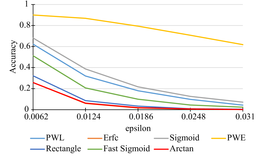
Figure 4: Accuracy of SEW ResNet on CIFAR 100 with respect to different gradient surrogates.

Figure 5: Accuracy of Vanilla Spiking ResNet on ImageNet with respect to different gradient surrogates.

Dataset	CIFAR-10				CIFAR-100				ImageNet
Model	S-R-BP	S-V-BP	S-V-T10	S-V-T5	S-R-BP	S-V-BP	S-V-T10	S-V-T5	S-R-BP	S-V-T5
Timesteps	4	20	10	5	5	30	10	5	4	5

Table 11: The timesteps used for each SNN model we used in the paper

CIFAR-10
	Arctan	PWL	Erfc	Sigmoid	PWE	Rectangle	Fast Sigmoid
MIM	37.6%	37.0%	36.9%	39.0%	21.9%	41.0%	18.5%
PGD	38.0%	35.9%	37.4%	37.0%	23.2%	38.7%	18.3%
AutoPGD	55.4%	54.5%	54.4%	55.5%	40.4%	56.0%	34.1%
CIFAR-100
	Arctan	PWL	Erfc	Sigmoid	PWE	Rectangle	Fast Sigmoid
MIM	46.6%	44.9%	47.1%	47.5%	35.9%	48.9%	29.7%
PGD	49.6%	43.9%	46.4%	46.3%	36.8%	47.5%	30.9%
AutoPGD	64.3%	61.7%	63.1%	63.4%	53.0%	64.0%	44.8%

Table 12: White box attack success rate for ResNet-18 SNN model with DM adversarial training method on CIFAR 10, CIFAR 100 with respect to different surrogate gradients.

CIFAR-10
	Arctan	PWL	Erfc	Sigmoid	PWE	Rectangle	Fast Sigmoid
MIM	46.4%	45.9%	45.9%	46.8%	28.5%	49.3%	25.2%
PGD	47.9%	45.9%	47.1%	46.8%	27.7%	45.9%	25.6%
AutoPGD	73.0%	71.5%	72.3%	73.2%	54.6%	69.7%	55.1%
CIFAR-100
	Arctan	PWL	Erfc	Sigmoid	PWE	Rectangle	Fast Sigmoid
MIM	69.8%	70.7%	70.4%	71.0%	55.6%	70.5%	50.4%
PGD	69.2%	69.6%	71.1%	69.2%	54.3%	69.1%	49.4%
AutoPGD	90.4%	90.6%	90.6%	90.1%	84.9%	88.7%	82.2%

Table 13: White box attack success rate for ResNet-18 SNN model with FAT adversarial training method on CIFAR 10, CIFAR 100 with respect to different surrogate gradients.

CIFAR-10
	Arctan	PWL	Erfc	Sigmoid	PWE	Rectangle	Fast Sigmoid
FGSM	85.1%	83.9%	83.9%	84.8%	82.9%	81.9%	79.8%
MIM	99.8%	99.8%	99.8%	99.8%	99.3%	99.8%	97.5%
PGD	100.0%	99.9%	100.0%	100.0%	99.7%	99.9%	98.3%
AutoPGD	100.0%	100.0%	100.0%	100.0%	100.0%	100.0%	99.7%
CIFAR-100
	Arctan	PWL	Erfc	Sigmoid	PWE	Rectangle	Fast Sigmoid
FGSM	89.9%	89.7%	90.1%	90.3%	89.0%	88.4%	85.4%
MIM	99.6%	99.5%	99.6%	99.6%	98.8%	99.6%	94.7%
PGD	99.7%	99.7%	99.7%	99.7%	99.3%	99.6%	96.3%
AutoPGD	100.0%	100.0%	100.0%	100.0%	99.8%	99.9%	99.1%

Table 14: White box attack success rate for ResNet-19 SNN model with TIC adversarial training method on CIFAR 10, CIFAR 100 with respect to different surrogate gradients.

CIFAR-10
	Arctan	PWL	Erfc	Sigmoid	PWE	Rectangle	Fast Sigmoid	STDB
MIM	46.4%	45.9%	45.9%	46.8%	28.5%	49.3%	25.2%	94.8%
PGD	47.9%	45.9%	47.1%	46.8%	27.7%	45.9%	25.6%	96.4%
AutoPGD	73.0%	71.5%	72.3%	73.2%	54.6%	69.7%	55.1%	98.5%
CIFAR-100
	Arctan	PWL	Erfc	Sigmoid	PWE	Rectangle	Fast Sigmoid	STDB
MIM	69.8%	70.7%	70.4%	71.0%	55.6%	70.5%	50.4%	65.8%
PGD	69.2%	69.6%	71.1%	69.2%	54.3%	69.1%	49.4%	69.1%
AutoPGD	90.4%	90.6%	90.6%	90.1%	84.9%	88.7%	82.2%	68.0%

Table 15: White box attack success rate for VGG-16 SNN on CIFAR 10 and VGG-11 SNN on CIFAR 100 with HIRE adversarial training method with respect to different surrogate gradients.

Appendix C Adversarial Trained SNNs Supplementary Material

To further validate the substantial influence of the surrogate gradient estimator, we consolidate four state-of-the-art adversarial training (AT) methods and conduct training on SNNs to study in our paper. Specifically, we modify two new effective adversarial training methods from CNN domain, namely DM (Wang et al. 2023) and FAT (Zhang et al. 2020a), for SNN-specific training. Additionally, we introduce two newly proposed adversarial training methods for SNNs, denoted as HIRE (Kundu et al. 2021) and TIC (Kim et al. 2023). We adopt the AT for SNNs and perform FGSM, MIM, PGD, and AutoPGD on the trained SNNs with different surrogate gradient estimators.

DM (Wang et al. 2023) proposed to use class-conditional elucidating diffusion model (EDM) (Karras et al. 2022) to generate augmented datasets for CIFAR-10 and CIFAR-100, and use TRADES (Zhang et al. 2019) pipeline for adversarial training. This TRADES training utilizes a classification-calibrated loss theory to attain a differentiable upper bound, enhancing model accuracy while shifting the decision boundary from the data to boost robustness. To train our SEW ResNet18 SNNs on CIFAR-10 and CIFAR-100, we utilized TRADES5 with 10M and 1M augment data as per the original paper settings. Notably, this adversarial training yields the highest robustness among all investigated methods but achieves lowest model accuracy (66.8% for CIFAR-10 and 41.0% for CIFAR-100). The attack results are shown in Table 12.

Friendly adversarial training (FAT) (Zhang et al. 2020a) focuses on identifying adversarial data that minimizes loss. This method trains a DNN by minimizing the loss with wrongly-predicted adversarial data and maximizing the loss with correctly-predicted adversarial data. The implementation employs early-stopped PGD for ease of adaptation. We maintain consistency with the original paper’s approach by employing PGD-10-5 to train SEW ResNet18 SNNs on CIFAR-10 (73.2%) and CIFAR-100 (40.8%). While the trained SNNs demonstrate some level of robustness, it is not as potent as observed in (Wang et al. 2023). The attack results are detailed in Table 13.

Temporal Information Concentration (TIC) (Kim et al. 2023) highlights that in SNNs, the information gradually shifts from later timesteps to earlier timesteps during training. This phenomenon is investigated in this study, where they estimate the Fisher information of the weights and propose a loss function to regulate the trend of Fisher information in SNNs. The adversarial training approximates the relationship between the loss function and Fisher information, pushing the loss value towards a specific target $\alpha$. Following the guidance provided in the paper, we train ResNet19 SNNs with $\alpha=1e-3$ for CIFAR-10 and $\alpha=1e-4$ for CIFAR-100. Although the SNNs achieve high accuracy (92.3% and 72.1%), as stated in the paper, their robustness is not strong, even when different estimators are used, as indicated in Table 14.

HIRE-SNN (Kundu et al. 2021) represents a spike timing dependent backpropagation (STDB) driven SNN training algorithm aimed at enhancing the inherent robustness of SNNs. The approach is tailored to conversion-based SNN training and prioritizes the optimization of model trainable parameters. This is achieved by introducing crafted noise to perturb pixel values across time steps in images. Our implementation follows the original paper’s methodology, dividing time steps into two equal-length intervals and introducing input noise after each period during training. For CIFAR-10 and CIFAR-100 datasets, we trained VGG-16 (89.0%) and VGG-11 (66.1%), respectively. Although the SNNs achieve higher accuracy, they demonstrate very low robustness when the correct surrogate gradient estimator is chosen, as shown in Table 15.

Appendix D Auto-SAGA Supplementary Material

Here we list the attack settings for experiments shown in Section Auto-SAGA Experimental Results. For all attacks, we use a maximum perturbation of $\epsilon=0.031$ with respect to the $l_{\infty}$ norm.

1. For single MIM and PGD attacks, we use $\epsilon_{step}=0.01$, attack step = 40 to generate AEs from each model, and list the highest attack success rate on each pair of the models.

2. For basic SAGA, we set the attack as a balanced version of SAGA that uses coefficients $\alpha_{1}=\alpha_{2}=0.5$ for two models to generate AEs and get the attack success rate among both models.

3. As for Auto-SAGA, we set learning rate $r=10,000$ for the coefficients. We set attack step = 40 and $\epsilon_{step}=0.005$ to generate AEs.

Model 1	Model 2	Max MIM	Max PGD	Max Auto	Basic SAGA	Auto-SAGA
C-V	S-R-BP	40.7%	33.6%	40.4%	49.8%	93.2%
C-V	S-V-BP	59.4%	51.3%	57.6%	67.2%	94.7%
C-V	S-V-T10	73.1%	68.6%	70.3%	78.6%	84.0%
C-V	S-R-T10	69.6%	46.6%	68.5%	84.4%	91.8%
S-R-BP	S-V-T10	41.7%	33.7%	29.8%	45.3%	64.3%
V-L16	S-R-BP	28.3%	23.5%	22.1%	74.5%	78.9%
V-L16	S-V-BP	33.9%	20.3%	18.8%	70.0%	85.4%
V-L16	S-V-T10	25.7%	15.3%	13.6%	33.0%	91.5%
V-L16	S-R-T10	27.2%	17.4%	15.3%	60.8%	93.8%
C-101x3	S-R-BP	38.3%	32.6%	30.3%	52.0%	77.3%
C-101x3	S-V-BP	22.7%	16.9%	16.1%	57.0%	83.8%
C-101x3	S-V-T10	24.6%	20.3%	17.9%	44.5%	84.5%
C-101x3	S-R-T10	25.2%	21.0%	19.5%	85.8%	97.0%

Table 16: Max MIM, PGD, and Auto represent the max suc- cess rate using adversarial examples generated by model 1 and model 2 for CIFAR-100 task

Model 1	Model 2	Max MIM	Max PGD	Max Auto	Basic SAGA	Auto-SAGA
TIC-R19	HIRE-V11	68.5%	69.0%	66.1%	15.2%	72.9%
FAT-R18	HIRE-V11	28.3%	29.6%	28.5%	21.7%	50.1%
FAT-R18	TIC-R19	25.2%	25.5%	27.1%	23.8%	46.6%
DM-R18	HIRE-V11	14.8%	16.0%	17.7%	14.6%	38.0%
DM-R18	FAT-R18	27.9%	27.7%	29.5%	29.7%	37.4%
DM-R18	TIC-R19	12.1%	11.2%	11.5%	11.7%	35.8%

Table 17: Max MIM, PGD, and Auto represent the max success rate using adversarial examples generated by adversarial trained SNN model 1 and model 2 for CIFAR-100 task.

Appendix E SNN Transferability Study Supplementary Material

	S-R-BP	S-V-BP	S-V-T5	S-V-T10	S-R-T5	S-R-T10	VB32	VB16	VL16	C-V	C-R	R101x3
S-R-BP	92.00%	19.30%	18.30%	17.10%	21.10%	18.00%	8.70%	5.60%	4.80%	19.60%	20.10%	5.00%
S-V-BP	15.30%	89.90%	46.20%	46.60%	51.80%	51.50%	10.10%	9.80%	6.50%	44.00%	52.30%	12.20%
S-V-T5	14.20%	45.10%	60.10%	96.80%	54.90%	55.80%	8.70%	9.20%	6.50%	76.10%	53.40%	13.30%
S-V-T10	13.60%	42.40%	98.00%	57.60%	52.90%	52.30%	8.50%	9.10%	6.30%	73.70%	51.50%	12.10%
S-R-T5	10.10%	25.50%	29.70%	29.50%	48.70%	85.30%	4.10%	4.40%	3.70%	28.60%	57.50%	6.60%
S-R-T10	11.70%	38.80%	47.10%	48.90%	97.80%	68.40%	8.80%	8.50%	6.40%	41.60%	79.30%	12.80%
VB32	10.70%	14.40%	15.60%	15.50%	21.90%	20.50%	100.00%	83.70%	75.10%	13.00%	20.30%	60.40%
VB16	8.90%	11.90%	11.70%	11.50%	18.90%	17.40%	57.40%	100.00%	88.90%	10.60%	16.80%	42.90%
VL16	8.10%	10.00%	13.40%	14.10%	19.60%	16.70%	55.30%	87.00%	99.00%	9.90%	15.20%	44.20%
C-V	14.40%	65.40%	98.10%	98.60%	78.80%	82.50%	13.80%	14.90%	10.90%	83.90%	83.10%	21.50%
C-R	15.20%	67.20%	74.60%	74.00%	98.30%	99.10%	15.40%	20.00%	13.70%	82.20%	98.30%	29.30%
R101x3	8.50%	7.30%	7.10%	7.50%	11.80%	9.80%	8.60%	20.00%	12.30%	6.10%	9.70%	100.00%

Table 18: Transferability results for CIFAR-10. The first column in represents the model used to generate the adversarial examples, $C_{i}$. The top row in represents the model used to evaluate the adversarial examples, $C_{j}$. Each entry is the maximum transferability computed using $C_{i}$ and $C_{j}$ over four different white-box attacks, Auto-PGD, MIM, PGD and FGSM using Equation 8. Transferability results for other datasets are given in the appendix. Model abbreviations are used for succinctness, S=SNN, R=ResNet, V=VGG-16, C=CNN, BP=Backpropagation, T denotes the Transfer SNN model with corresponding timestep and V=ViT.

FGSM
	S-R-BP	S-V-BP	S-V-T5	S-V-T10	S-R-T5	S-R-T10	VB32	VB16	VL16	C-V	C-R	R101x3
S-R-BP	78.90%	15.60%	12.60%	13.50%	18.90%	16.30%	6.90%	5.50%	4.00%	13.20%	16.50%	4.30%
S-V-BP	14.40%	64.10%	31.70%	31.60%	34.80%	36.50%	6.30%	6.20%	5.20%	28.80%	35.90%	6.90%
S-V-T5	14.20%	36.40%	49.70%	72.40%	45.70%	47.60%	8.00%	7.90%	6.50%	58.70%	42.70%	11.60%
S-V-T10	13.60%	35.80%	73.40%	51.20%	44.10%	45.50%	8.10%	9.00%	6.30%	58.20%	43.90%	10.60%
S-R-T5	9.40%	16.60%	17.50%	18.20%	24.40%	34.30%	4.10%	4.40%	2.80%	19.30%	30.10%	4.50%
S-R-T10	11.40%	26.00%	28.60%	28.70%	54.50%	39.80%	6.00%	6.90%	5.00%	29.70%	45.90%	8.20%
VB32	9.90%	13.20%	15.30%	13.50%	21.90%	20.50%	62.40%	43.80%	37.30%	12.90%	20.30%	29.40%
VB16	8.90%	11.90%	10.70%	10.70%	18.90%	17.40%	30.40%	60.60%	43.10%	10.60%	16.80%	25.30%
VL16	8.10%	10.00%	10.70%	10.30%	16.30%	16.70%	24.40%	38.40%	43.50%	9.90%	15.20%	19.20%
C-V	13.60%	47.60%	76.50%	80.20%	57.90%	57.70%	10.60%	11.90%	8.30%	58.80%	60.70%	12.60%
C-R	14.70%	50.00%	51.90%	53.60%	77.80%	66.10%	11.60%	14.70%	10.00%	52.40%	81.40%	15.90%
R101x3	8.50%	7.30%	7.10%	7.30%	11.80%	9.80%	3.20%	5.50%	3.30%	6.10%	9.70%	13.90%
PGD
	S-R-BP	S-V-BP	S-V-T5	S-V-T10	S-R-T5	S-R-T10	VB32	VB16	VL16	C-V	C-R	R101x3
S-R-BP	57.10%	14.80%	12.10%	12.20%	17.80%	14.50%	4.80%	3.20%	3.10%	13.30%	14.90%	3.00%
S-V-BP	10.90%	89.90%	31.30%	32.40%	38.60%	37.70%	4.60%	4.00%	2.60%	30.40%	39.00%	6.00%
S-V-T5	9.20%	34.90%	52.50%	85.20%	46.00%	48.60%	3.90%	3.50%	1.80%	67.80%	47.60%	6.90%
S-V-T10	10.60%	34.00%	92.30%	52.00%	45.20%	45.70%	4.40%	3.60%	2.30%	66.70%	45.40%	7.00%
S-R-T5	7.00%	11.40%	13.00%	12.60%	20.90%	48.20%	1.30%	1.30%	0.80%	13.30%	26.10%	2.20%
S-R-T10	9.00%	23.80%	30.30%	32.10%	85.90%	51.20%	2.50%	3.00%	1.80%	28.20%	60.00%	5.50%
VB32	7.30%	6.60%	5.00%	4.80%	8.80%	6.90%	97.60%	63.20%	39.30%	4.50%	5.30%	32.00%
VB16	5.80%	4.20%	2.70%	2.40%	5.60%	4.70%	14.80%	99.80%	56.80%	2.10%	2.90%	16.90%
VL16	5.90%	4.80%	3.70%	2.80%	6.80%	4.90%	20.40%	78.10%	92.40%	2.30%	3.20%	21.80%
C-V	11.50%	55.10%	94.40%	95.40%	70.80%	70.10%	7.70%	10.40%	6.30%	72.50%	72.80%	15.40%
C-R	11.80%	60.50%	64.60%	67.20%	97.10%	98.40%	11.00%	13.20%	8.10%	66.50%	89.60%	22.90%
R101x3	6.00%	4.40%	2.60%	1.60%	5.50%	2.50%	1.20%	2.70%	0.90%	2.00%	1.90%	100.00%
APGD
	S-R-BP	S-V-BP	S-V-T5	S-V-T10	S-R-T5	S-R-T10	VB32	VB16	VL16	C-V	C-R	R101x3
S-R-BP	67.50%	19.20%	18.30%	17.10%	21.10%	18.00%	8.70%	5.60%	4.80%	19.60%	20.10%	5.00%
S-V-BP	10.50%	63.60%	36.70%	36.70%	43.50%	42.80%	6.50%	6.80%	4.40%	37.10%	47.50%	8.00%
S-V-T5	9.70%	38.30%	59.40%	96.80%	54.90%	55.80%	3.50%	4.30%	2.30%	76.10%	52.60%	7.80%
S-V-T10	10.80%	35.00%	98.00%	54.90%	52.00%	51.30%	3.90%	4.10%	2.50%	73.70%	51.50%	8.40%
S-R-T5	8.80%	25.50%	29.70%	29.50%	48.70%	85.30%	3.00%	3.50%	2.20%	28.60%	57.50%	6.60%
S-R-T10	10.50%	36.40%	43.30%	43.90%	97.80%	68.40%	5.10%	5.80%	3.30%	38.90%	79.30%	9.80%
VB32	8.40%	8.20%	15.60%	15.50%	21.60%	16.50%	100.00%	70.50%	47.80%	6.10%	9.40%	40.40%
VB16	6.30%	6.80%	11.70%	11.50%	16.20%	11.80%	22.90%	100.00%	71.40%	3.80%	7.40%	25.50%
VL16	6.50%	6.10%	13.40%	14.10%	19.60%	13.20%	26.50%	87.00%	99.00%	5.80%	7.50%	26.90%
C-V	11.60%	65.40%	98.10%	98.60%	78.80%	82.50%	13.80%	14.30%	10.20%	83.90%	83.10%	21.50%
C-R	11.10%	66.10%	69.30%	71.90%	98.30%	99.10%	15.20%	17.20%	12.10%	82.20%	97.80%	29.30%
R101x3	7.70%	5.30%	6.80%	7.50%	11.40%	9.60%	3.30%	7.50%	3.30%	2.40%	4.10%	100.00%
MIM
	S-R-BP	S-V-BP	S-V-T5	S-V-T10	S-R-T5	S-R-T10	VB32	VB16	VL16	C-V	C-R	R101x3
S-R-BP	92.00%	19.30%	16.60%	15.40%	20.20%	16.20%	6.80%	5.10%	4.80%	15.50%	18.60%	4.30%
S-V-BP	15.30%	88.60%	46.20%	46.60%	51.80%	51.50%	10.10%	9.80%	6.50%	44.00%	52.30%	12.20%
S-V-T5	12.10%	45.10%	60.10%	80.90%	54.10%	55.50%	8.70%	9.20%	5.50%	67.80%	53.40%	13.30%
S-V-T10	13.00%	42.40%	89.10%	57.60%	52.90%	52.30%	8.50%	9.10%	5.70%	68.30%	51.10%	12.10%
S-R-T5	10.10%	23.10%	27.70%	27.80%	38.70%	66.40%	3.70%	4.40%	3.70%	26.60%	47.50%	4.80%
S-R-T10	11.70%	38.80%	47.10%	48.90%	88.20%	64.00%	8.80%	8.50%	6.40%	41.60%	72.90%	12.80%
VB32	10.70%	14.40%	13.30%	12.20%	20.90%	18.40%	95.90%	83.70%	75.10%	13.00%	18.20%	60.40%
VB16	7.50%	9.70%	11.10%	10.00%	14.40%	13.90%	57.40%	99.40%	88.90%	9.40%	14.30%	42.90%
VL16	7.90%	9.70%	9.10%	9.10%	14.80%	13.70%	55.30%	78.40%	91.60%	8.60%	13.20%	44.20%
C-V	14.40%	63.50%	94.50%	95.70%	73.40%	76.30%	12.80%	14.90%	10.90%	78.40%	77.70%	19.40%
C-R	15.20%	67.20%	74.60%	74.00%	96.10%	89.20%	15.40%	20.00%	13.70%	73.50%	98.30%	28.90%
R101x3	7.50%	7.20%	5.70%	4.90%	11.80%	7.70%	8.60%	20.00%	12.30%	5.60%	8.20%	100.00%

Table 19: Full transferability results for CIFAR-10. The first column in each table represents the model used to generate the adversarial examples, $C_{i}$. The top row in each table represents the model used to evaluate the adversarial examples, $C_{j}$. Each entry represents $T_{i,j}$ (the transferability) computed using Equation 4 with $C_{i}$, $C_{j}$ and either FGSM, PGD or MIM. For each attack the maximum perturbation bounds is $\epsilon=0.031$. Based on these results we take the maximum transferability across all attacks and report the result in Table 18. We also visually show the maximum transferability $t_{i,j}$ in Figure 2.

	S-R-BP	S-V-BP	S-V-T5	S-V-T10	S-R-T8	VB32	VB16	VL16	C-V	C-R	R101x3
S-R-BP	99.80%	53.80%	67.90%	67.50%	68.80%	67.00%	67.30%	74.30%	68.10%	73.10%	65.10%
S-V-BP	52.10%	68.90%	52.40%	54.40%	56.30%	82.90%	85.20%	88.20%	54.30%	60.80%	84.00%
S-V-T5	65.60%	54.10%	98.90%	96.90%	65.70%	83.50%	81.20%	88.10%	93.70%	60.10%	80.60%
S-V-T10	65.70%	54.10%	97.30%	98.60%	62.50%	83.40%	81.40%	85.90%	93.50%	58.30%	81.20%
S-R-T8	62.60%	49.00%	59.80%	59.90%	96.90%	80.80%	81.30%	87.00%	58.20%	84.70%	80.20%
VB32	78.80%	79.70%	83.90%	84.80%	81.80%	97.10%	88.50%	83.50%	85.70%	87.70%	61.20%
VB16	85.10%	82.90%	86.50%	87.10%	84.90%	71.00%	99.80%	93.30%	89.80%	89.70%	70.40%
VL16	82.80%	83.00%	85.30%	86.20%	84.40%	67.20%	88.40%	97.00%	88.70%	89.50%	64.00%
C-V	55.60%	58.70%	88.30%	88.10%	64.70%	71.40%	71.20%	78.90%	89.10%	63.40%	70.50%
C-R	54.00%	57.90%	68.50%	68.20%	92.80%	72.90%	72.00%	79.40%	69.00%	98.60%	71.90%
R101x3	88.30%	86.50%	90.70%	91.20%	85.80%	87.10%	76.70%	87.40%	92.70%	93.10%	99.30%
R101x3	8.50%	7.30%	7.10%	7.50%	11.80%	9.80%	8.60%	20.00%	12.30%	6.10%	9.70%

Table 20: Transferability results for CIFAR-100. The first column in each table represents the model used to generate the adversarial examples, $C_{i}$. The top row in each table represents the model used to evaluate the adversarial examples, $C_{j}$. Each entry is the maximum transferability computed using $C_{i}$ and $C_{j}$ with three different white-box attacks, MIM, PGD and FGSM using Equation 8. Model abbreviations are used for succinctness, S=SNN, -R=ResNet, -V=VGG-16, C=CNN, BP=Backpropagation, T denotes the Transfer SNN model with corresponding timestep and V=ViT.

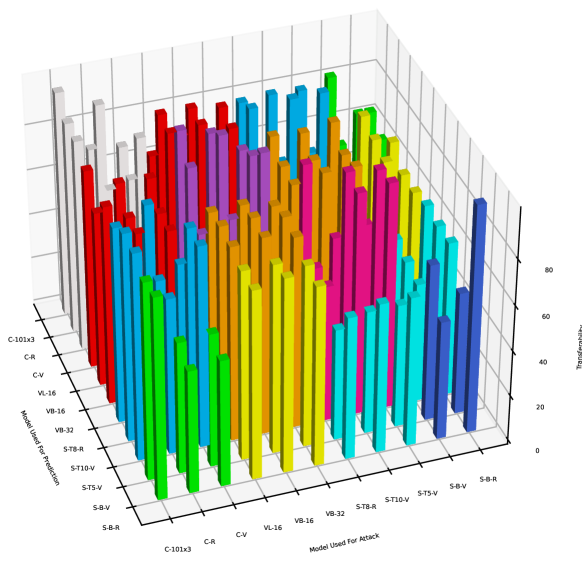
Figure 6: Visual representation of Table 20 for CIFAR-100. The x-axis corresponds to the model used to generate the adversarial examples. The y-axis corresponds to the model used to classify the adversarial examples. The z-axis corresponds to the transferability measurement (see Equation 4). The colors of the bars represent the measurements between different model types, e.g. yellow represents the transferability results between BP SNNs and ViTs.

FGSM
	S-R-BP	S-V-BP	S-V-T5	S-V-T10	S-R-T8	VB32	VB16	VL16	C-V	C-R	R101x3
S-R-BP	92.80%	41.90%	31.90%	28.40%	29.00%	22.10%	19.80%	14.00%	29.20%	26.10%	22.40%
S-V-BP	42.80%	51.10%	40.90%	41.20%	38.50%	15.30%	13.90%	9.60%	38.80%	35.60%	15.20%
S-V-T5	39.10%	44.30%	87.90%	82.90%	50.10%	19.10%	18.20%	14.20%	78.10%	46.60%	17.80%
S-V-T10	38.40%	46.10%	82.10%	87.30%	49.60%	19.30%	20.10%	14.60%	78.40%	44.10%	18.80%
S-R-T8	31.50%	37.50%	44.00%	44.90%	79.70%	14.70%	14.40%	10.80%	42.20%	62.90%	15.50%
VB32	35.30%	32.10%	27.30%	27.30%	27.40%	79.00%	59.80%	58.30%	22.90%	22.90%	42.10%
VB16	28.70%	27.00%	26.60%	27.20%	26.70%	49.30%	79.40%	63.30%	23.20%	23.30%	38.20%
VL16	31.40%	27.60%	26.20%	24.30%	26.50%	43.00%	58.30%	65.70%	22.70%	21.80%	34.60%
C-V	43.30%	52.30%	81.20%	81.00%	56.90%	24.60%	25.00%	17.80%	84.00%	53.90%	24.50%
C-R	40.30%	47.20%	55.40%	53.30%	79.20%	19.60%	19.40%	15.50%	54.30%	86.90%	19.40%
R101x3	16.90%	20.30%	21.50%	19.10%	23.60%	14.80%	16.50%	14.30%	17.90%	17.10%	36.20%
R101x3	0.085	0.073	0.071	0.073	0.118	0.098	0.032	0.055	0.033	0.061	0.097
PGD
	S-R-BP	S-V-BP	S-V-T5	S-V-T10	S-R-T8	VB32	VB16	VL16	C-V	C-R	R101x3
S-R-BP	99.80%	44.20%	27.80%	25.00%	27.10%	25.00%	23.00%	16.90%	26.60%	23.90%	23.40%
S-V-BP	36.00%	57.30%	38.20%	36.40%	35.70%	10.50%	10.30%	6.50%	36.30%	31.70%	10.90%
S-V-T5	29.80%	46.80%	98.90%	96.90%	55.00%	12.00%	13.80%	9.80%	93.60%	51.70%	13.60%
S-V-T10	29.70%	45.70%	97.30%	98.60%	54.00%	12.40%	13.80%	9.30%	93.50%	50.90%	14.90%
S-R-T8	23.10%	36.40%	49.80%	51.20%	96.50%	8.50%	9.60%	6.10%	47.50%	80.10%	11.30%
VB32	15.90%	14.60%	11.70%	10.20%	13.70%	97.10%	74.10%	56.80%	7.80%	5.70%	37.60%
VB16	10.30%	13.80%	7.70%	7.60%	11.80%	30.40%	99.80%	76.40%	4.60%	3.70%	21.50%
VL16	11.30%	10.40%	7.90%	7.80%	12.10%	34.90%	87.10%	97.00%	5.40%	4.80%	28.50%
C-V	37.10%	53.80%	88.30%	88.10%	60.00%	19.20%	20.60%	14.50%	89.10%	57.50%	21.40%
C-R	37.40%	53.50%	66.40%	65.80%	92.80%	18.10%	19.20%	14.10%	67.80%	98.60%	20.70%
R101x3	7.70%	10.30%	7.40%	5.40%	12.80%	6.20%	10.40%	5.20%	3.80%	3.10%	99.20%
V-L16	6.9%	5.6%	5.2%	3.6%	7.0%	5.8%	21.5%	2.4%	2.9%	18.2%	77.8%
APGD
	S-R-BP	S-V-BP	S-V-T5	S-V-T10	S-R-T8	VB32	VB16	VL16	C-V	C-R	R101x3
S-R-BP	0.00%	48.70%	67.90%	67.50%	68.80%	67.00%	67.30%	74.30%	68.10%	73.10%	65.10%
S-V-BP	52.10%	26.70%	52.40%	54.40%	56.30%	82.90%	85.20%	88.20%	54.30%	60.80%	84.00%
S-V-T5	65.60%	46.60%	0.10%	0.70%	34.80%	83.50%	81.20%	88.10%	4.30%	39.90%	80.60%
S-V-T10	65.70%	48.80%	0.70%	0.10%	37.50%	83.40%	81.40%	85.90%	5.20%	46.00%	81.20%
S-R-T8	62.60%	44.30%	30.60%	31.50%	0.20%	80.80%	81.30%	87.00%	32.80%	7.30%	80.20%
VB32	78.80%	79.70%	83.90%	84.80%	81.80%	0.00%	20.30%	34.70%	85.70%	87.70%	54.90%
VB16	85.10%	82.90%	86.50%	87.10%	84.90%	57.60%	0.00%	16.60%	89.80%	89.70%	70.40%
VL16	82.80%	83.00%	85.30%	86.20%	84.40%	52.90%	7.60%	0.00%	88.70%	89.50%	64.00%
C-V	55.60%	39.40%	9.60%	9.70%	33.20%	71.40%	71.20%	78.90%	9.00%	35.10%	70.50%
C-R	54.00%	33.80%	23.90%	24.50%	3.00%	72.90%	72.00%	79.40%	24.00%	0.50%	71.90%
R101x3	88.30%	86.50%	90.70%	91.20%	85.80%	87.10%	76.70%	87.40%	92.70%	93.10%	0.00%
V-L16	7.70%	6.70%	9.20%	5.00%	9.20%	7.60%	28.60%	4.70%	8.00%	26.20%	86.20%
MIM
	S-R-BP	S-V-BP	S-V-T5	S-V-T10	S-R-T8	VB32	VB16	VL16	C-V	C-R	R101x3
S-R-BP	99.70%	53.80%	38.00%	34.10%	33.60%	31.00%	27.80%	22.00%	34.60%	31.20%	30.50%
S-V-BP	52.00%	68.90%	52.30%	50.60%	49.40%	21.80%	20.10%	14.20%	50.60%	44.20%	19.20%
S-V-T5	39.80%	54.10%	98.20%	96.60%	65.70%	21.60%	21.60%	16.50%	93.70%	60.10%	20.90%
S-V-T10	40.10%	54.10%	96.10%	97.60%	62.50%	20.10%	21.40%	16.90%	92.80%	58.30%	22.40%
S-R-T8	33.20%	49.00%	59.80%	59.90%	96.90%	18.80%	17.70%	13.20%	58.20%	84.70%	19.20%
VB32	32.20%	25.40%	23.40%	21.80%	21.70%	96.20%	88.50%	83.50%	20.20%	18.30%	61.20%
VB16	21.20%	21.20%	18.50%	19.90%	19.90%	71.00%	99.00%	93.30%	15.50%	15.30%	47.10%
VL16	24.20%	23.40%	19.20%	18.70%	20.40%	67.20%	88.40%	95.10%	15.30%	14.90%	50.00%
C-V	43.90%	58.70%	87.30%	87.50%	64.70%	27.10%	27.30%	19.00%	88.20%	63.40%	26.40%
C-R	42.70%	57.90%	68.50%	68.20%	92.70%	23.60%	23.60%	18.00%	69.00%	97.50%	22.80%
R101x3	15.40%	17.40%	15.30%	14.20%	15.50%	25.60%	38.30%	27.10%	12.40%	11.60%	99.30%
V-L16	6.7%	8.2%	7.6%	6.7%	11.2%	9.2%	45.4%	6.5%	8.4%	54.4%	77.7%

Table 21: Full transferability results for CIFAR-100. The first column in each table represents the model used to generate the adversarial examples, $C_{i}$. The top row in each table represents the model used to evaluate the adversarial examples, $C_{j}$. Each entry represents $T_{i,j}$ (the transferability) computed using Equation 4 with $C_{i}$, $C_{j}$ and either FGSM, PGD or MIM. For each attack the maximum perturbation bounds is $\epsilon=0.031$. Based on these results we take the maximum transferability across all attacks and report the result in Table 20. We also visually show the maximum transferability $t_{i,j}$ in Figure 6.

References

- Abnar et al. (2020) Abnar, S.; and Zuidema, W. 2020. Quantifying Attention Flow in Transformers. In Proceedings of the 58th Annual Meeting of the Association for Computational Linguistics, 4190–4197.
- Athalye et al. (2018) Athalye, A.; Carlini, N.; and Wagner, D. 2018. Obfuscated Gradients Give a False Sense of Security: Circumventing Defenses to Adversarial Examples. In Proceedings of the 35th International Conference on Machine Learning, 274–283.
- Bellec et al. (2018) Bellec, G.; Salaj, D.; Subramoney, A.; Legenstein, R.; and Maass, W. 2018. Long short-term memory and learning-to-learn in networks of spiking neurons. Advances in neural information processing systems, 31.
- Bengio et al. (2013) Bengio, Y.; Léonard, N.; and Courville, A. 2013. Estimating or propagating gradients through stochastic neurons for conditional computation. arXiv preprint arXiv:1308.3432.
- Carlini et al. (2017) Carlini, N.; and Wagner, D. 2017. Towards evaluating the robustness of neural networks. In 2017 ieee symposium on security and privacy (sp), 39–57. Ieee.
- Croce et al. (2020) Croce, F.; and Hein, M. 2020. Reliable evaluation of adversarial robustness with an ensemble of diverse parameter-free attacks. In International conference on machine learning, 2206–2216. PMLR.
- Davies et al. (2018) Davies, M.; Srinivasa, N.; Lin, T.-H.; Chinya, G.; Cao, Y.; Choday, S. H.; Dimou, G.; Joshi, P.; Imam, N.; Jain, S.; et al. 2018. Loihi: A neuromorphic manycore processor with on-chip learning. Ieee Micro, 38(1): 82–99.
- Davies et al. (2021) Davies, M.; Wild, A.; Orchard, G.; Sandamirskaya, Y.; Guerra, G. A. F.; Joshi, P.; Plank, P.; and Risbud, S. R. 2021. Advancing neuromorphic computing with loihi: A survey of results and outlook. Proceedings of the IEEE, 109(5): 911–934.
- Diehl et al. (2015) Diehl, P. U.; Neil, D.; Binas, J.; Cook, M.; Liu, S.-C.; and Pfeiffer, M. 2015. Fast-classifying, high-accuracy spiking deep networks through weight and threshold balancing. In 2015 International joint conference on neural networks (IJCNN), 1–8. ieee.
- Dong et al. (2018) Dong, Y.; Liao, F.; Pang, T.; Su, H.; Zhu, J.; Hu, X.; and Li, J. 2018. Boosting adversarial attacks with momentum. In Proceedings of the IEEE conference on computer vision and pattern recognition (CVPR), 9185–9193.
- Dosovitskiy et al. (2020) Dosovitskiy, A.; Beyer, L.; Kolesnikov, A.; Weissenborn, D.; Zhai, X.; Unterthiner, T.; Dehghani, M.; Minderer, M.; Heigold, G.; Gelly, S.; et al. 2020. An Image is Worth 16x16 Words: Transformers for Image Recognition at Scale. In International Conference on Learning Representations.
- El-Allami et al. (2021) El-Allami, R.; Marchisio, A.; Shafique, M.; and Alouani, I. 2021. Securing deep spiking neural networks against adversarial attacks through inherent structural parameters. In 2021 Design, Automation & Test in Europe Conference & Exhibition (DATE), 774–779. IEEE.
- Fang et al. (2020a) Fang, H.; Mei, Z.; Shrestha, A.; Zhao, Z.; Li, Y.; and Qiu, Q. 2020a. Encoding, model, and architecture: Systematic optimization for spiking neural network in fpgas. In 2020 IEEE/ACM International Conference On Computer Aided Design (ICCAD), 1–9. IEEE.
- Fang et al. (2020b) Fang, H.; Shrestha, A.; Zhao, Z.; and Qiu, Q. 2020b. Exploiting neuron and synapse filter dynamics in spatial temporal learning of deep spiking neural network. In 29th International Joint Conference on Artificial Intelligence, IJCAI 2020, 2799–2806. International Joint Conferences on Artificial Intelligence.
- Fang et al. (2021a) Fang, W.; Yu, Z.; Chen, Y.; Huang, T.; Masquelier, T.; and Tian, Y. 2021a. Deep residual learning in spiking neural networks. Advances in Neural Information Processing Systems, 34: 21056–21069.
- Fang et al. (2021b) Fang, W.; Yu, Z.; Chen, Y.; Masquelier, T.; Huang, T.; and Tian, Y. 2021b. Incorporating learnable membrane time constant to enhance learning of spiking neural networks. In Proceedings of the IEEE/CVF International Conference on Computer Vision, 2661–2671.
- Goodfellow et al. (2015) Goodfellow, I.; Shlens, J.; and Szegedy, C. 2015. Explaining and Harnessing Adversarial Examples. In International Conference on Learning Representations.
- Goodfellow et al. (2014) Goodfellow, I. J.; Shlens, J.; and Szegedy, C. 2014. Explaining and harnessing adversarial examples. arXiv preprint arXiv:1412.6572.
- He et al. (2016) He, K.; Zhang, X.; Ren, S.; and Sun, J. 2016. Deep residual learning for image recognition. In Proceedings of the IEEE conference on computer vision and pattern recognition, 770–778.
- Horowitz (2014) Horowitz, M. 2014. 1.1 computing’s energy problem (and what we can do about it). In 2014 IEEE International Solid-State Circuits Conference Digest of Technical Papers (ISSCC), 10–14. IEEE.
- Karras et al. (2022) Karras, T.; Aittala, M.; Aila, T.; and Laine, S. 2022. Elucidating the design space of diffusion-based generative models. Advances in Neural Information Processing Systems, 35: 26565–26577.
- Kim et al. (2023) Kim, Y.; Li, Y.; Park, H.; Venkatesha, Y.; Hambitzer, A.; and Panda, P. 2023. Exploring temporal information dynamics in spiking neural networks. In Proceedings of the AAAI Conference on Artificial Intelligence, volume 37, 8308–8316.
- Kolesnikov et al. (2020) Kolesnikov, A.; Beyer, L.; Zhai, X.; Puigcerver, J.; Yung, J.; Gelly, S.; and Houlsby, N. 2020. Big Transfer (BiT): General Visual Representation Learning. Lecture Notes in Computer Science, 491–507.
- Krizhevsky et al. (2009) Krizhevsky, A.; Hinton, G.; et al. 2009. Learning multiple layers of features from tiny images.
- Krizhevsky et al. (2012) Krizhevsky, A.; Sutskever, I.; and Hinton, G. E. 2012. Imagenet classification with deep convolutional neural networks. In Advances in neural information processing systems, 1097–1105.
- Kugele et al. (2020) Kugele, A.; Pfeil, T.; Pfeiffer, M.; and Chicca, E. 2020. Efficient processing of spatio-temporal data streams with spiking neural networks. Frontiers in Neuroscience, 14: 439.
- Kundu et al. (2021) Kundu, S.; Pedram, M.; and Beerel, P. A. 2021. Hire-snn: Harnessing the inherent robustness of energy-efficient deep spiking neural networks by training with crafted input noise. In Proceedings of the IEEE/CVF International Conference on Computer Vision, 5209–5218.
- Liang et al. (2021) Liang, L.; Hu, X.; Deng, L.; Wu, Y.; Li, G.; Ding, Y.; Li, P.; and Xie, Y. 2021. Exploring adversarial attack in spiking neural networks with spike-compatible gradient. IEEE transactions on neural networks and learning systems.
- Liu et al. (2016) Liu, Y.; Chen, X.; Liu, C.; and Song, D. 2016. Delving into transferable adversarial examples and black-box attacks. arXiv preprint arXiv:1611.02770.
- Lu et al. (2020) Lu, S.; and Sengupta, A. 2020. Exploring the connection between binary and spiking neural networks. Frontiers in Neuroscience, 14: 535.
- Madry et al. (2018) Madry, A.; Makelov, A.; Schmidt, L.; Tsipras, D.; and Vladu, A. 2018. Towards Deep Learning Models Resistant to Adversarial Attacks. In International Conference on Learning Representations.
- Mahmood et al. (2021a) Mahmood, K.; Gurevin, D.; van Dijk, M.; and Nguyen, P. 2021a. Beware the Black-Box: On the Robustness of Recent Defenses to Adversarial Examples. Entropy, 23: 1359.
- Mahmood et al. (2021b) Mahmood, K.; Mahmood, R.; and Van Dijk, M. 2021b. On the robustness of vision transformers to adversarial examples. In Proceedings of the IEEE/CVF International Conference on Computer Vision, 7838–7847.
- Mahmood et al. (2022) Mahmood, K.; Nguyen, P. H.; Nguyen, L. M.; Nguyen, T.; and Van Dijk, M. 2022. Besting the Black-Box: Barrier Zones for Adversarial Example Defense. IEEE Access, 10: 1451–1474.
- Neftci et al. (2019) Neftci, E. O.; Mostafa, H.; and Zenke, F. 2019. Surrogate gradient learning in spiking neural networks: Bringing the power of gradient-based optimization to spiking neural networks. IEEE Signal Processing Magazine, 36(6): 51–63.
- Rathi et al. (2021) Rathi, N.; and Roy, K. 2021. DIET-SNN: A low-latency spiking neural network with direct input encoding and leakage and threshold optimization. IEEE Transactions on Neural Networks and Learning Systems.
- Rathi et al. (2020) Rathi, N.; Srinivasan, G.; Panda, P.; and Roy, K. 2020. Enabling Deep Spiking Neural Networks with Hybrid Conversion and Spike Timing Dependent Backpropagation. In International Conference on Learning Representations.
- Rueckauer et al. (2022) Rueckauer, B.; Bybee, C.; Goettsche, R.; Singh, Y.; Mishra, J.; and Wild, A. 2022. NxTF: An API and compiler for deep spiking neural networks on Intel Loihi. ACM Journal on Emerging Technologies in Computing Systems (JETC), 18(3): 1–22.
- Sharmin et al. (2019) Sharmin, S.; Panda, P.; Sarwar, S. S.; Lee, C.; Ponghiran, W.; and Roy, K. 2019. A comprehensive analysis on adversarial robustness of spiking neural networks. In 2019 International Joint Conference on Neural Networks (IJCNN), 1–8. IEEE.
- Sharmin et al. (2020) Sharmin, S.; Rathi, N.; Panda, P.; and Roy, K. 2020. Inherent adversarial robustness of deep spiking neural networks: Effects of discrete input encoding and non-linear activations. In European Conference on Computer Vision, 399–414. Springer.
- Shrestha et al. (2022) Shrestha, A.; Fang, H.; Mei, Z.; Rider, D. P.; Wu, Q.; and Qiu, Q. 2022. A Survey on Neuromorphic Computing: Models and Hardware. IEEE Circuits and Systems Magazine, 22(2): 6–35.
- Shrestha et al. (2018) Shrestha, S. B.; and Orchard, G. 2018. Slayer: Spike layer error reassignment in time. Advances in neural information processing systems, 31.
- Simonyan et al. (2014) Simonyan, K.; and Zisserman, A. 2014. Very deep convolutional networks for large-scale image recognition. arXiv preprint arXiv:1409.1556.
- Szegedy et al. (2013) Szegedy, C.; Zaremba, W.; Sutskever, I.; Bruna, J.; Erhan, D.; Goodfellow, I.; and Fergus, R. 2013. Intriguing properties of neural networks. arXiv preprint arXiv:1312.6199.
- Tang et al. (2020) Tang, G.; Kumar, N.; and Michmizos, K. P. 2020. Reinforcement co-learning of deep and spiking neural networks for energy-efficient mapless navigation with neuromorphic hardware. In 2020 IEEE/RSJ International Conference on Intelligent Robots and Systems (IROS), 6090–6097. IEEE.
- Tavanaei et al. (2019) Tavanaei, A.; Ghodrati, M.; Kheradpisheh, S. R.; Masquelier, T.; and Maida, A. 2019. Deep learning in spiking neural networks. Neural networks, 111: 47–63.
- Tramer et al. (2020) Tramer, F.; Carlini, N.; Brendel, W.; and Madry, A. 2020. On adaptive attacks to adversarial example defenses. Advances in Neural Information Processing Systems, 33: 1633–1645.
- Wang et al. (2023) Wang, Z.; Pang, T.; Du, C.; Lin, M.; Liu, W.; and Yan, S. 2023. Better diffusion models further improve adversarial training. arXiv preprint arXiv:2302.04638.
- Wu et al. (2018) Wu, Y.; Deng, L.; Li, G.; Zhu, J.; and Shi, L. 2018. Spatio-temporal backpropagation for training high-performance spiking neural networks. Frontiers in neuroscience, 12: 331.
- Wu et al. (2019) Wu, Y.; Deng, L.; Li, G.; Zhu, J.; Xie, Y.; and Shi, L. 2019. Direct training for spiking neural networks: Faster, larger, better. In Proceedings of the AAAI Conference on Artificial Intelligence, volume 33, 1311–1318.
- Zenke et al. (2018) Zenke, F.; and Ganguli, S. 2018. Superspike: Supervised learning in multilayer spiking neural networks. Neural computation, 30(6): 1514–1541.
- Zenke et al. (2021) Zenke, F.; and Vogels, T. P. 2021. The remarkable robustness of surrogate gradient learning for instilling complex function in spiking neural networks. Neural computation, 33(4): 899–925.
- Zhang et al. (2019) Zhang, H.; Yu, Y.; Jiao, J.; Xing, E.; El Ghaoui, L.; and Jordan, M. 2019. Theoretically principled trade-off between robustness and accuracy. In International conference on machine learning, 7472–7482. PMLR.
- Zhang et al. (2020a) Zhang, J.; Xu, X.; Han, B.; Niu, G.; Cui, L.; Sugiyama, M.; and Kankanhalli, M. 2020a. Attacks which do not kill training make adversarial learning stronger. In International conference on machine learning, 11278–11287. PMLR.
- Zhang et al. (2020b) Zhang, W.; and Li, P. 2020b. Temporal spike sequence learning via backpropagation for deep spiking neural networks. Advances in Neural Information Processing Systems, 33: 12022–12033.
- Zheng et al. (2021) Zheng, H.; Wu, Y.; Deng, L.; Hu, Y.; and Li, G. 2021. Going deeper with directly-trained larger spiking neural networks. In Proceedings of the AAAI Conference on Artificial Intelligence, volume 35, 11062–11070.