Modeling FETCH Observations of a Coronal Mass Ejection

Abstract

This paper evaluates the quality of CME analysis that has been undertaken with the rare Faraday rotation observation of an eruption. Exploring the capability of the FETCH instrument hosted on the MOST mission, a four-satellite Faraday rotation radio sounding instrument deployed between the Earth and the Sun, we discuss the opportunities and challenges to improving the current analysis approaches.

1 Introduction

1.1 History

Coronal mass ejections produce the largest-scale disturbances in the heliosphere. As they approach Earth, CME magnetic ejecta may extend over 0.25 AU and the CME-driven shock may extend twice as far. For example, the intensity of the 2005 May CME disturbance is impressive at 1 AU with velocities approaching 2000 km/s, magnetic fields observed at over 100 nT and plasma densities at 50 protons $cm^{-3}$, magnitudes which range from 5 to 10 times ambient solar wind values.

As such, these disturbances possess both the scale and intensity that strongly affect radio wave propagation through the heliosphere, which in turn allows for remote sensing of these extraordinary events. CMEs have been imaged with Thomson-scattered white light within 1AU (and beyond) by both the Solar Terrestrial Relations Observatory (STEREO) heliographic imagers (Howard et al., 2008) and Solar Mass Ejection Imager (SMEI) (Eyles et al., 2003) spacecraft.

Ground-based radio wave scintillation has long been used to infer both the plasma density and velocity of CMEs with tomographic analysis providing the 3D maps of these quantities (Jackson et al., 2004, 2006).

The first Faraday rotation (FR) observations of the heliosphere were conducted in 1968 by Pioneer 6 (Levy et al., 1969)). The observed FR curve was ’W’-shaped with rotation angles of 40 degrees recorded over a period of 2–3 hr that have been attributed to a coronal streamer stalk (Woo, 1997) or the passage of a series of CMEs (Pätzold & Bird, 1998). Jensen and Russell (Jensen & Russell, 2008) modeled these structures as CMEs; however, as discovered in Jensen et al. (Jensen et al., 2018), these structures share the jagged characteristics of reconnection regions (discussed in the last section of this paper). Unusual Faraday rotation structures contained within CMEs were observed with Helios spacecraft (October/November 1979). Around this time, we were discovering that unusual magnetic structures observed in the solar wind were Earth-crossing CMEs (e.g. see discussion in Mulligan dissertation–reference).

Rapid growth in ground-based radio astronomical instruments, especially with the development of the Karl G. Jansky Very Large Array (VLA) and the Robert C. Byrd Green Bank Telescope (GBT), opened the door to a new generation of CME FR observations. Spangler & Whiting (2009) reported the serendipitous detection of CME FR ($\mathrm{RM}\approx 10.9\,\mathrm{rad}\,\mathrm{m}^{-2}$) during 1.465 GHz VLA observations made by Ingleby et al. (2007) of background radio galaxies. Jensen et al. (2018 references) collected high time cadence FR observations of MESSENGER and with GBT. Howard et al. (2016) detected a relatively weak CME FR signal ($\mathrm{RM}\approx 3.6-4.3\,\mathrm{rad}\,\mathrm{m}^{-2}$) using a pulsar; however, this was comparable to the local ionospheric FR ($\mathrm{RM}\approx 1.5-2.5\,\mathrm{rad}\,\mathrm{m}^{-2}$) and, thus, they only provided upper limits on the plasma density and magnetic field parameters for this CME.

Kooi et al. (2017) detected FR through two CMEs in August 2012 by observing background radio galaxies with the newly upgraded VLA’s full $1-2$ GHz L-band. These CME observations were unique because

• the southern CME (in heliographic latitude) was constrained by both radio FR and white-light coronagraph observations;

• the northern CME is the only CME with plasma parameters constrained by radio FR, white-light coronagraph, and in situ observations.

Wood et al. (2020) generated 3-D morphological reconstructions of both CMEs using the white-light coronagraph data; combining these with the radio FR and in situ data, they determined the CME flux rope’s plasma density, magnetic field strength, and magnetic field orientation, even for the southern CME, which lacked in situ data. Kooi et al. (2021) later demonstrated that the magnetic field strength and orientation can also be determined from radio FR observations alone, provided multiple lines-of-sight (LOS) are available to sample different regions of the CME structure. This was discussed by Jensen et al. (2010 reference) as the approach necessary to eliminate the handedness-orientation ambiguity.

Beyond the magnetic flux rope core, CME characteristics in FR observations have largely been absent. The MESSENGER CME observation (Jensen et al, 2018) showed little to no sheath region. However, unlike previous spacecraft observations, this was the first to calculate the full Stokes parameters. When the bursty plasma trailing the CME crossed the line-of-sight (LOS), it was clearly not a CME, due to the signal polarization amplitude changes within. The Helios CME observations (Bird, 1985) were fit with flux rope geometries (Jensen, 2008), but as we show in this paper, the sheath region was beginning to develop on these and should now be taken into consideration.

Jensen et al (2010) discussed the disadvantage to studying CME magnetic configurations with FR observing at the Earth. The sheath region in particular obscures the orientation of the magnetic flux rope. Observations of the rope need to be collected close to the solar surface simultaneously on both sides of the Sun prior to the development of the sheath region, or as discussed here regarding the FETCH configuration, a different angle of observing needs to be achieved altogether.

For a thorough review of modern observations of CME FR, see Kooi et al. (2022) and references therein.

1.2 CMEs

3D numerical simulations of CMEs allows the opportunity to simulate Faraday rotation observations in a wide variety of circumstances. Liu et al. (2007) simulated FR observations from the idealized 3D CME simuation of Manchester IV et al. (2004) from a number of points of view and found that a significant signal could be obtained, which would provide the flux rope helicity. In this study, we used a much more realistic simulation of the CME observed to erupt from the Sun on 2005 May 13 (Manchester IV et al., 2014), which provides much more structure.

Once an ICME is more than 40 solar radii from the Sun, it will begin to deform as the wind acceleration slows and the ICME interacts with streams of different speed (Manchester et al., 2017). Portions of the CME impacting slow solar wind propagate slower than regions extending into fast wind, resulting in Sun-ward indentations in CME-driven shocks and potentially bending the ICME flux rope into a outward concave configuration (Manchester IV et al., 2004, 2005). The aspect ratio also increases as a CME propagates away from the Sun as first noted by Riley et al. (2004).

Open questions regarding CMEs that FR and signal polarization investigations can address include:

• (1) do all have flux ropes? Nearly 50% of ICMEs have the form of well-defined magnetic clouds (Burlaga, 1994; Richardson & Cane, 2010; Manchester et al., 2017)

• (2) evolution, azimuthal expansion is less than expected

• (3) magnetic field

Understanding the plasma structure of CMEs and their evolution through space is crucial to understanding space weather. Space weather is a critical field of study in both the civilian and military sectors of government. In recent years, the U.S. federal government has issued a series of directives to strengthen space weather research, e.g. the 2021 U.S. Space Priorities Framework states that “The United States will enhance the protection of terrestrial critical infrastructure from space weather events, which can disrupt services such as electric power, telecommunications, water supply, health care, and transportation.” A recent analysis by the Congressional Budget Office (CBO) estimated that federal agencies participating in the Space Weather Operations, Research, and Mitigation (SWORM) Working Group, “allocated a combined total of nearly $350 million to activities related to space weather” in FY2019 (Lipiec & Humphreys, 2020).

1.3 MOST/FETCH

The Multiview Observatory for Solar Terrestrial Science (MOST) mission seeks to understand the magnetic coupling of the solar interior to the heliosphere (Gopalswamy et al., 2022). Composed of 4 spacecraft, 2 hosting 10 instruments in the Lagrange L4 and L5 positions and 2 hosting the FETCH instrument alone at larger angular offsets from Earth, MOST will be the most comprehensive solar mission to date. The locations of its deployed spacecraft are chosen to improve on STEREO’s work observing upstream from the Earth and L1, but with the new technology (FETCH) of remotely observing the magnetic field in the Earthbound solar wind as well.

FETCH consists of four radio Lines-Of-Sight (LOS) for measuring the electron density, magnetic field parameters, and velocity parameters crossing the LOS’s as shown in Figure 1. FETCH is a radio sounding instrument, detecting the modifications that a controlled signal undergoes due to the plasma through which it is traversing. FETCH’s cutting edge technology is its being the first to pass signals from spacecraft to spacecraft across 2 AU, and with the greatest sensitivity in the signal (the lowest offset point) occurring where the Earth-bound solar wind plasma is passing the LOSs. As we discuss in more detail below, the signal characteristics of frequency, phase, polarization, amplitude, and spectral distribution are combined to measure FR, TEC, Faraday Rotation Fluctuations (FRF), and Frequency Fluctuations (FF) using established techniques (e.g. Jensen et al., 2018; Wexler et al., 2017; Efimov et al., 2000; Imamura et al., 2014).

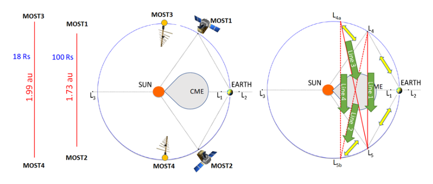
Figure 1: Overview of the MOST mission with the four constituent spacecraft at L4 (MOST1), L5 (MOST2), ahead of L4 (L4a, MOST3) and behind L5 (L5b, MOST4). MOST3&4 will carry only radio equipment for Faraday rotation measurement (FETCH). MOST1&2 will have identical remote-sensing and in-situ instrument suites. The approximate MOST1-MOST2 an MOST3-MOST4 distances are shown at the left indicating the long signal paths for spacecraft radio signals (blue text shows the offset distance to the point-of-closest-approach between the LOS and the Sun). The red lines in the right indicate FETCH signal paths; the green arrows label these paths Line1-4 and give the forward directions. This enables a rudimentary radio tomographic image using Faraday rotation Fung et al. (2022). The yellow double arrows indicate communication links to Earth. Note that MOST3&4 slowly shift position between L4&5 and the locations shown throughout the MOST mission

There continues to be open questions regarding the solar wind. For example: What is the radial profile of shock-driving coronal mass ejections (CMEs)? What is the internal magnetic structure of CMEs that cause magnetic storms? How do CMEs and corotating/stream interaction regions (CIRs/SIRs) evolve in the inner heliosphere? It is clear many of these questions involve solar magnetic fields at in various layers in of the solar atmosphere, and we have poor knowledge of them. In order to better understand the origin of variability in the solar wind plasma, it is necessary to probe the magnetic field in Earth-directed structures/disturbances.

The focus of the MOST mission and the FETCH instrument is not specifically CMEs; however, this paper is focused on developing FETCH’s CME capabilities. CMEs are important to understand not just for societal risks but also to understand the variability and dynamics of these large plasma structures (Manchester et al., 2017). We simulated a FETCH deployment within the AWSoM Heliospheric CME MHD simulation for the 13 May 2005 CME (Manchester et al., 2014). This simulation revealed FETCH capabilities and challenges to the analysis of CME observations, and this paper introduces and discusses these results.

Note for this study that while the signals will be travelling both ways between spacecraft to measure the LOSs between them vary over the 16 minute light time, we are not resolving/exploiting this tomographic capability as described in Fung et al (2022) in this paper. This is introduced in the Future Work section.

1.4 FR and Polarization

Faraday rotation analysis of linearly polarized signals provides information on the LOS-integrated product of electron number density ($n_{e}$) and LOS-aligned component of the magnetic field ($\overrightarrow{B}\cdot d\overrightarrow{S}$). In the regime where the radio frequency ($f_{0}$) is well above the electron plasma frequency, the Faraday rotation, given as the change in plane of polarization position angle, $\Delta\chi$ is expressed as

$$\Delta\chi=\frac{A}{f_{0}^{2}}\int n_{e}\overrightarrow{B}\cdot d\overrightarrow{S}$$ (1)

With $A=2.36\times 10^{4}$ $radm^{2}T^{-1}s^{-2}$. A convention that we commonly use to express Faraday rotation is to normalize it by wavelength $\lambda^{2}$ to calculate the Rotation Measure $RM=\Delta\chi/\lambda^{2}$. Faraday Rotation is the measure of the change in the position angle of the plane of polarization, which requires specifying a frequency. Rotation Measure (RM) enables comparing the Faraday Rotation among different frequencies.

The plane of polarization is measured using Stokes Parameters. Stokes parameters are the I, Q, U, and V characteristics of the signal; these are measured from the real and imaginary amplitudes of the signals received by the orthogonal elements of the FETCH antenna (a cross-dipole log periodic antenna). Recall that the phase of the signal is given by its real and imaginary components.

The frequency-shift, or apparent-Doppler tracking, method relies on measuring the frequency of a transmitted signal through a gradient in column density (Jensen et al., 2016). It is independent of Doppler motion that results from the spacecraft traveling towards/away from the receiver $dS/dt$. For a given frequency, f, the frequency shift, $\Delta f$ is given by

$$\frac{\Delta f}{f}=-\frac{1}{c}\frac{dS}{dt}+\frac{q_{e}^{2}}{2\omega^{2}c\epsilon_{0}m_{e}}\frac{d}{dt}TEC$$ (2)

Where $q_{e}$ is the electron charge, $\omega$ is the signal frequency in radians/second, $c$ is the speed of light, $\epsilon_{0}$ is the permittivity of free space, and $m_{e}$ is the electron mass. After removal of the Doppler shift component (by modeling or observing another frequency simultaneously), the residual frequency shifts can be integrated to obtain a measure of column density change or tracked to follow the trend in column density variability. For complete description of the electron density on the LOS, the baseline offset factor needs to be added from white-light data when using the apparent-Doppler shift method.

The fundamental challenge with Faraday rotation and TEC observing is the ability to decouple the parallel magnetic field and the density and their distribution along the LOS. The first order approach is to assume that they are evenly distributed relative to each other and to calculate $B_{p}\approx\Delta\chi/TEC\times f_{0}^{2}/A$. As shown in Figure 16 Panel 3R, this has an average error around a factor of 2. Using models and/or observing conditions which enable tomographic calculations, the decoupling can be significantly improved. In this paper, we will analyze the results of the first order approach as it is more common due to the paucity of regular FR observing opportunities. This gives error bars on these calculations.

1.5 Purpose

This study investigates the opportunities and challenges the FETCH instrument concept will have in observing CMEs. We simulated the FR, TEC, and velocity of an Earth-directed CME crossing the FETCH radio sensing paths. The necessary LOS modeled data, magnetic field, density, and velocity, along each LOS was obtained from the AWSoM heliospheric 3-D MHD model.

The May 13 2005 CME erupted from the north-south polarity inversion line of AR 10759 at 16:03 UT, reaching speeds around 2000 km/s in the corona. It was selected for this study because the ICME that resulted impacted the Earth’s geospace at around 1000 km/s with peak magnetic field (axial) strength of around 60 nT. The geomagnetic storm that was produced by the event produced a severe geomagnetic storm.

2 Methods

2.1 MHD Simulation: Model Data

Here, we summarize the magnetohydrodynamic (MHD) simulation of the 2005 May 13 CME event, which is originally described in Manchester IV et al. (2014). This CME and ambient solar wind are simulated with the Alfven Wave Solar Model (AWSoM) van der Holst et al. (2010); Oran et al. (2015); Sokolov et al. (2013); van der Holst et al. (2014), which provides a realistic three-dimensional (3D) description of the solar wind from the transition region to beyond 1AU. Transport processes include field-aligned heat conduction and radiation. The AWSoM model also includes a non-equilibrium multi-species approach that separately addresses the temperature of electrons and ions and allows the ionization of the plasma to be based on electron temperature Meng et al. (2015). In this way, the ion and electron temperatures are allowed to depart over the short times scales characteristic of reconnection and shock/wave propagation Manchester IV et al. (2012).

In the AWSoM model, the coronal heating and solar wind acceleration are driven with low-frequency Alfvén wave turbulence. A simple phenomenological turbulence formulation of wave energy transport with local turbulence dissipation is applied. The Alfvén waves emanate from the bottom boundary and propagate parallel to magnetic field lines. In this original model, wave reflection was parameterized by means of a reflection coefficient $C_{\rm l}03$ that prescribed the ratio of returning and outward propagating waves uniformly. Wave dissipation is driven by the mixing of forward and counter propagating waves, with balanced turbulence, optimal near the tops of closed loops. The dissipation depends on the correlation length $L_{\perp}$ that we assign inversely proportional to $\sqrt{B}$: $L_{\perp}\sqrt{B}=7.5\times 10^{4}$. Following, we prescribe 40% of the turbulently dissipated energy to electron heating, while the remaining 60% heats the protons.

Our coronal model for Carrington rotation 2029, which includes NOAA active region (AR) 10759 from which the CME erupts. The computational domain is divided into two components, a solar corona (SC), which extends to $24R_{s}$ and an inner heliosphere (IH) domain which extends from $22R_{s}$ to 2 AU. The SC employs a spherical adaptive grid with extremely high refinement in the transition region $(\delta r\approx 0.001R_{s})$, and much larger cells $(\delta r\approx 0.25R_{s})$ near the outer boundary located at $24R_{s}$. A cone-shaped region of enhanced refinement is centered on the AR 10759 with resolution four times higher than the standard model.

The CME is initiated with a Gibson-Low spheromak flux rope (Gibson & Low, 1998), which is linearly superimposed upon the existing corona so that the mass and magnetic field of the flux rope are added directly to AR 10759. The flux rope axis and its associated polarity inversion line (PIL) runs north-south, parallel to the observed polarity inversion line of AR 10759. The model mimics the classical three-part structure from which CMEs originate Hundhausen (1993). The magnetic field strength reaches a maximum value of 40-50 Gauss, which extends high into the corona in a non-potential configuration.

In the low corona, the flux rope rapidly accelerates to speeds of approximately 2000 km/s driving a fast-mode MHD shock ahead of the CME. After 1 hour, the flux rope has reach 15 $R_{s}$ and it structure resembles a magnetic cloud following self-similar evolution of the initial state. Eventually, this self-similar behavior breaks down as magnetic reconnection between the flux rope and ambient solar wind sets in. Reconnection at the bottom front and top rear sides opens up the flux rope, which is followed by a later phase of reconnection at the backside of flux rope. By 24 hours, the flux rope is turned with its axis nearly perpendicular to the solar equatorial plane as seen in Figure 2. The CME simulation for this event maintained the magnetic cloud structure with elevated magnetic field strength and reduced temperature & mass density. The north-south Bz polarities remain from the original flux rope at 1 AU, even though the original rope structure has been greatly modified by reconnection. (Manchester IV et al., 2014)

While the CME speed matches observations one hour after initiation, the model ICME is significantly slower at Earth with a speed of 600 km/s compared to the observed 950 km/s. Here, the excessive deceleration of the simulated CME is due to the density of the solar wind being roughly a factor of two too large, which also increases the rotation measure. The solar wind density has been remedied in more recent models, which show close agreement with observations (van der Holst et al., 2014; Sachdeva et al., 2019, 2021).

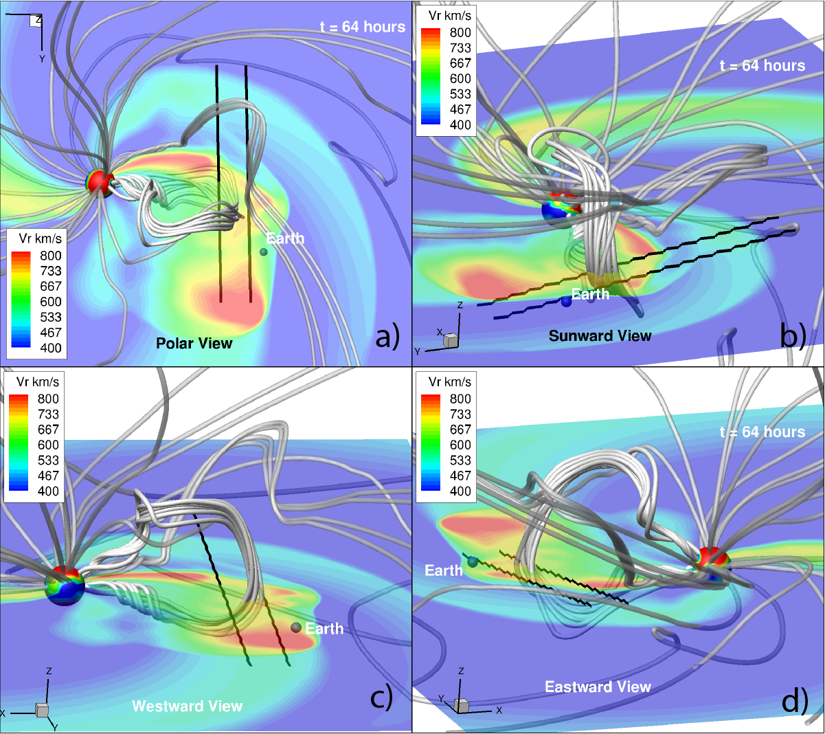
Figure 2: 3D renderings of the CME simulation of the May 13 2005 event 64 hours after initiation with radio propagation lines of sight. Here, we show the CME with magnetic field lines and the solar equatorial plane colored to show the plasma radial velocity. Panels (a)-(d) show respectively views from above the north pole, Sunward from the direction of Earth and westward and eastward facing perspectives.

2.2 Simulated in-situ Fits

At the locations of the CME’s crossing each line of sight, in-situ data was simulated from the AWSoM 2005 model (shown in black triangles in Figure 11. From these time series in proton/electron density, magnetic field orientation, velocity, and proton/electron temperatures, we determined the Leading-Edge (LE), Trailing-Edge(TE), and orienation of the magnetic flux rope. The Magnetic-Flux-Rope (MFR) used specifically is considered to be an axially symmetric magnetic helical structure with distorted cross-section Nieves-Chinchilla et al. (2022). The Elliptic-cylindrical (EC) model is a physics-driven model that assume elliptical cross-section but does not impose any condition on the internal magnetic forces. It assumes that the radial variation of the current density J can be expressed as a generic polynomial function.

The reconstruction is based on a multiple regression technique to infer the spacecraft trajectory using the Levenberg–Marquardt algorithm. This is an iterative exercise going from the local fluxrope coordinate system to the spacecraft coordinate system. The outcomes from the reconstruction are the flux rope orientation, distortion, and physical parameters, such as the central magnetic field and force-freeness.

Two Figures are generated for each in-situ time series at the LOS impact parameter. Figures 3, 4, 5, and 6 display all observations, magnetic field (GSE coordinates) and plasma data. It includes the FF boundaries (dotted line) and MFR-fit boundaries (dashed line). The criteria for placing the LE and TE are based on temperature, beta plasma, bulk velocity and the magnetic field rotation (see hodograms). The magnetic field strength indicates a bit of compression at the back of the structure. From Line 4 to Line 1, there is an increase in the magnetic field strength after the flux rope.

Figures 7, 8, 9, and 10 include the magnetic field and the fitting. Output parameters from the fit are shown above. All LOSs are consistent; the structure is highly inclined and as shown in the value of $q$. The Line 4 azimuth $F$ is different to the rest of the events, but it just indicates that the structure rotated a bit. There is not a big distortion; also the model does not capture the compression at the back. The magnetic field components are very well captured though.

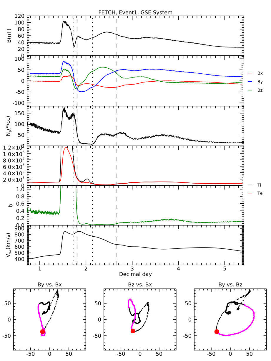
Figure 3: in-situ time series at the LOS impact parameter. Magnetic field, density, temperature, plasma beta, and velocity are shown with time. The hodograms below show the flux rope in pink. The dotted lines show the FF boundaries and the dashed lines show the boundaries based on plasma.

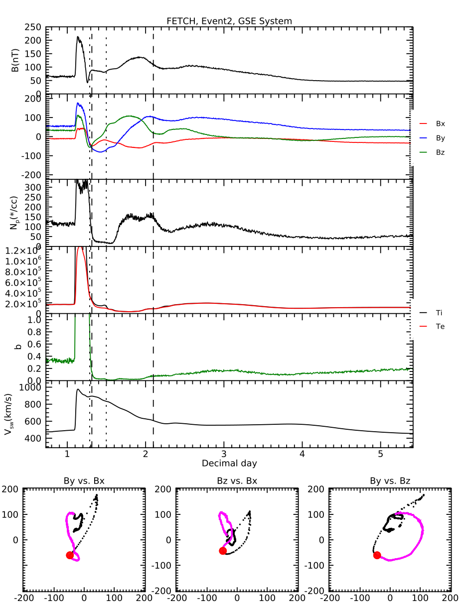
Figure 4: in-situ time series at the LOS impact parameter. Magnetic field, density, temperature, plasma beta, and velocity are shown with time. The hodograms below show the flux rope in pink. The dotted lines show the FF boundaries and the dashed lines show the boundaries based on plasma.

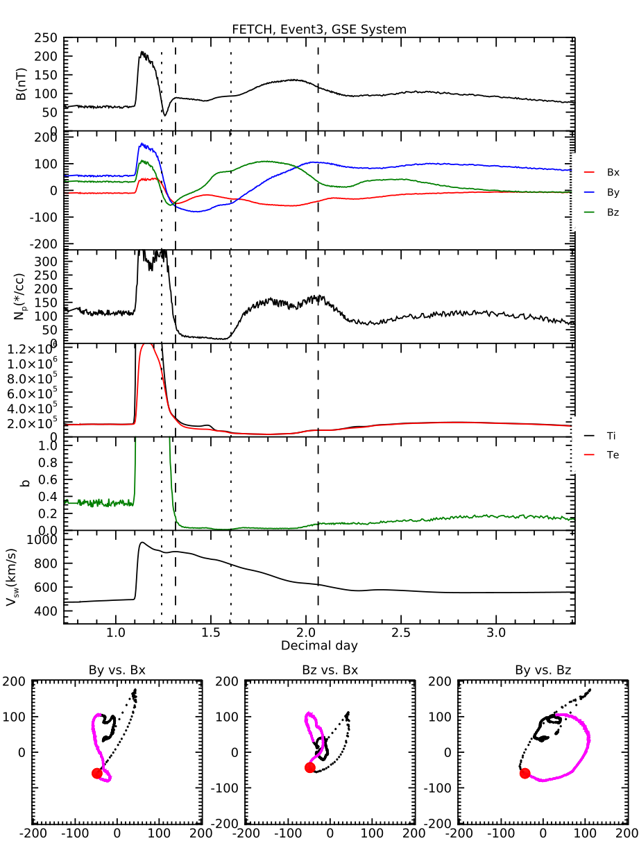
Figure 5: in-situ time series at the LOS impact parameter. Magnetic field, density, temperature, plasma beta, and velocity are shown with time. The hodograms below show the flux rope in pink. The dotted lines show the FF boundaries and the dashed lines show the boundaries based on plasma.

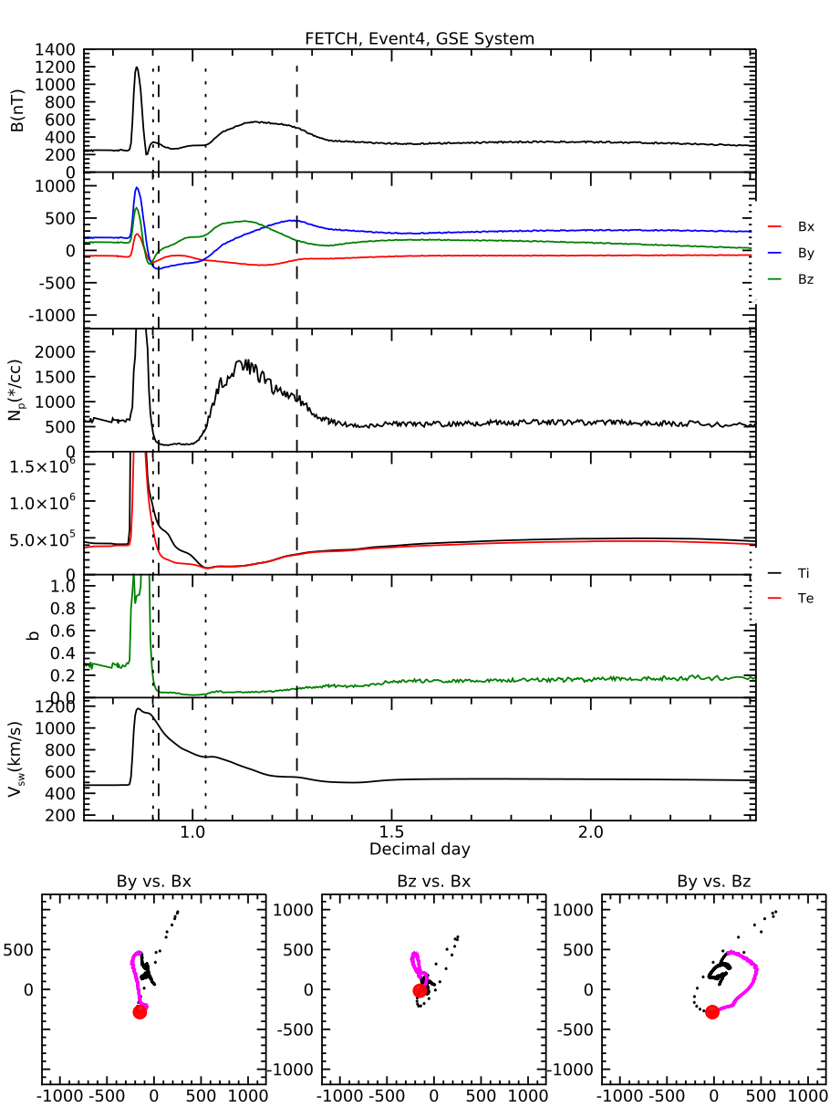
Figure 6: in-situ time series at the LOS impact parameter. Magnetic field, density, temperature, plasma beta, and velocity are shown with time. The hodograms below show the flux rope in pink. The dotted lines show the FF boundaries and the dashed lines show the boundaries based on plasma.

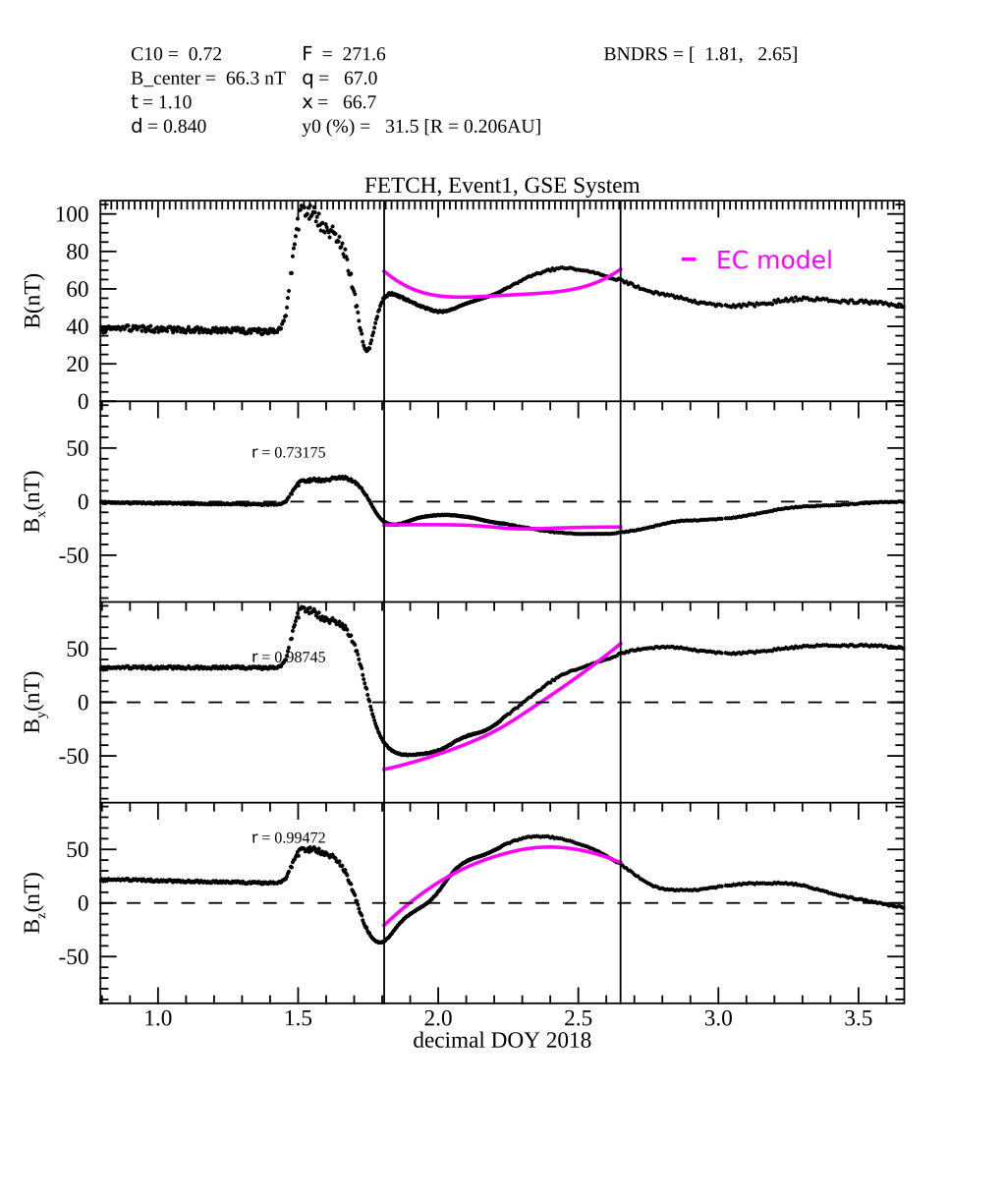
Figure 7: F is the azimuth in degrees, q is the latitude $\theta$ in degrees…

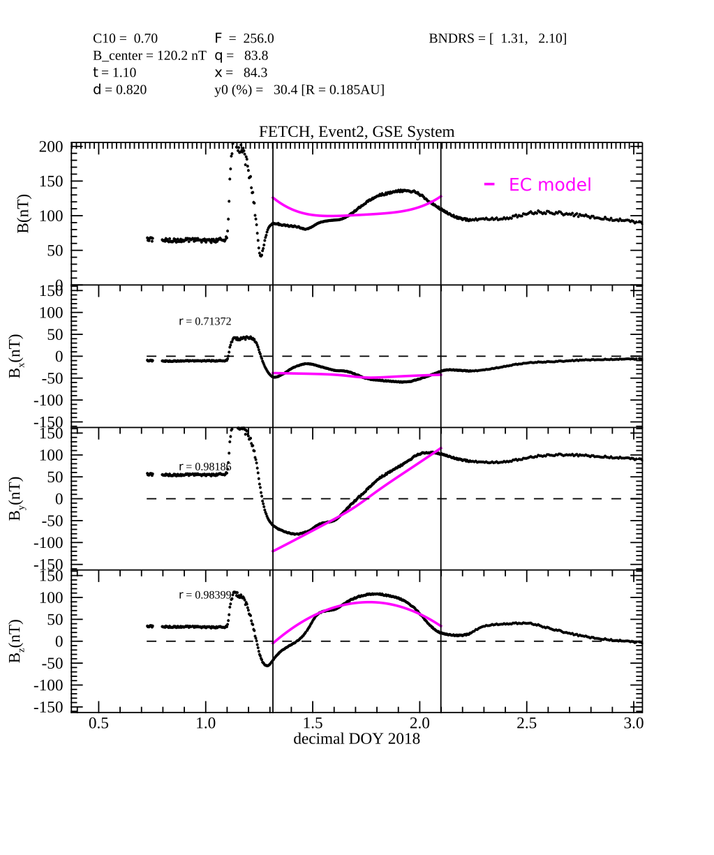
Figure 8: F is the azimuth in degrees, q is the latitude $\theta$ in degrees…

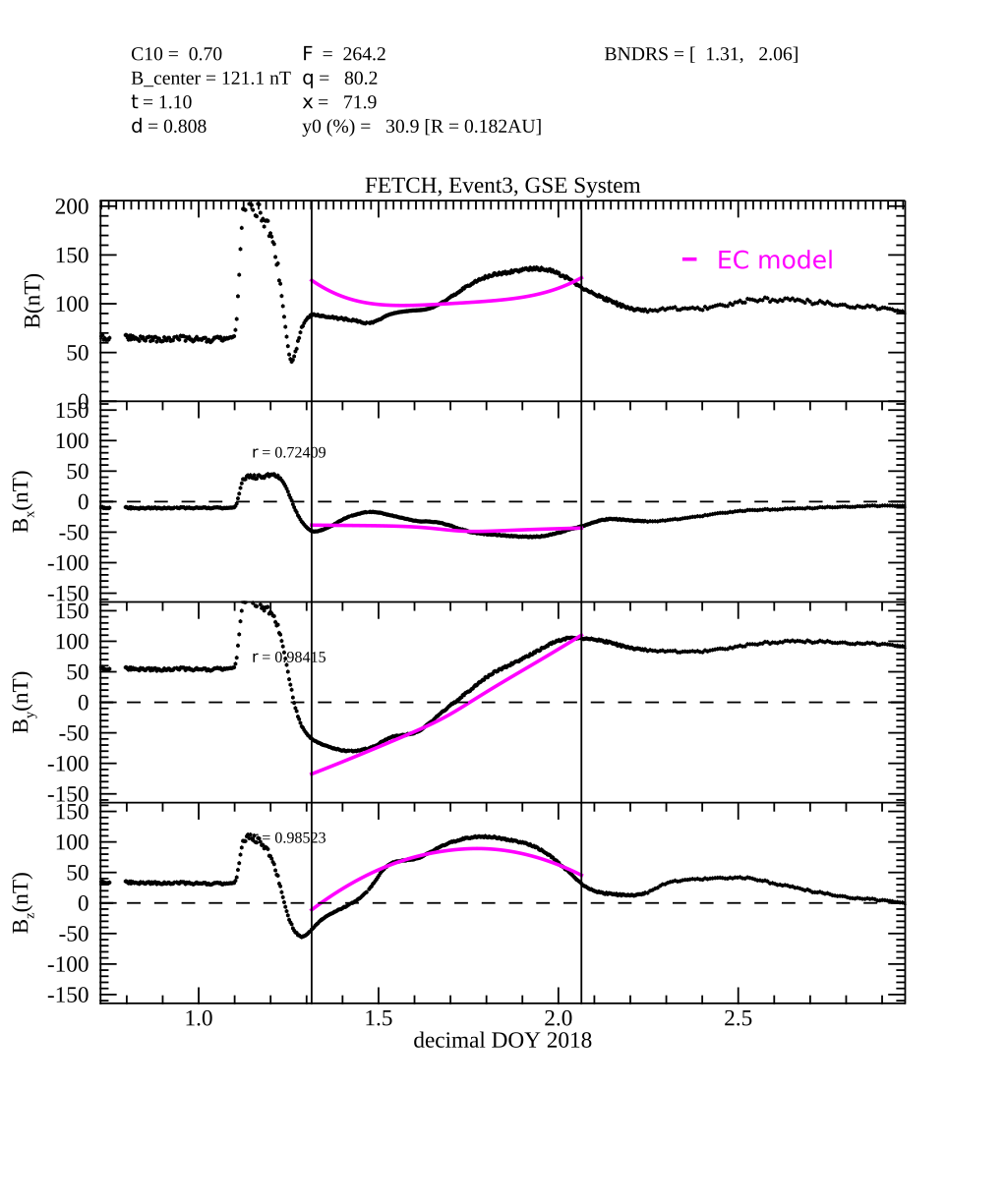
Figure 9: F is the azimuth in degrees, q is the latitude $\theta$ in degrees…

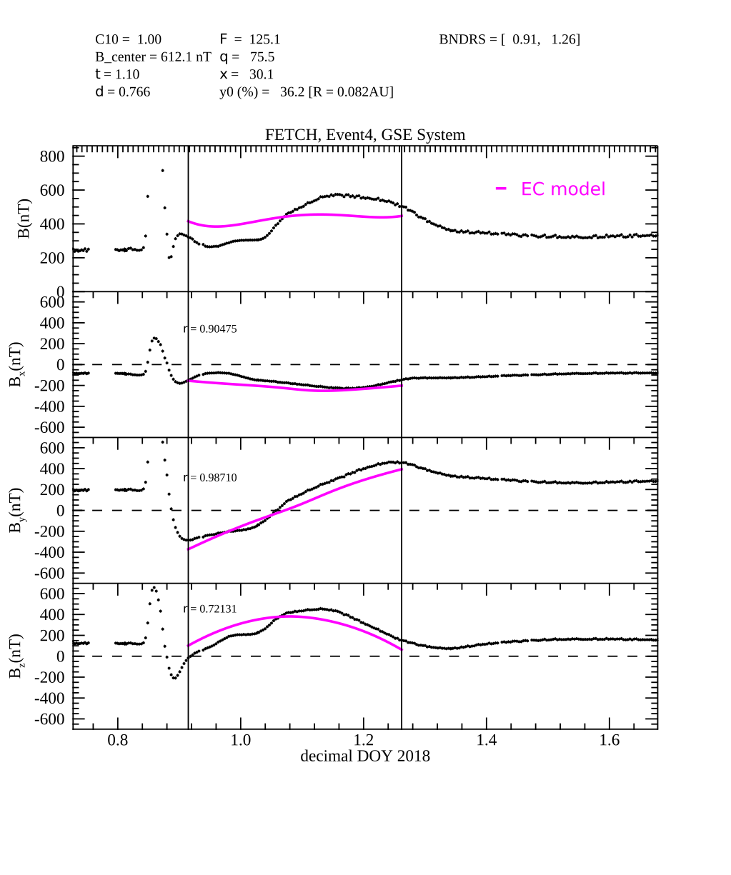
Figure 10: F is the azimuth in degrees, q is the latitude $\theta$ in degrees…

2.3 FR analysis of the Simulation

The locations of MOST 3 and 4 are variable. For this simulation, they were set to Line 4 (see Figure 1 LOS Line 4) having a minimum offset of 30 solar radii from the Sun. Much of time during the MOST primary mission places these spacecraft in this location.

Noise was added to the simulation model to examine the reliability of the results. Alfvén wave energy from the AWSoM model ($E_{w}$ expressed in $erg/cc$) was used to calculate the fluctuations in magnetic field strength with the equation $\sqrt{8\pi E_{w}}$. The fluctuations were varied randomly by 10% to add an uncertainty error bar to the subsequent fits. Likewise, the density was estimated to vary by around 10%, from Parker Solar Probe in-situ proton measurements. This was determined using the analysis attached in Appendix A. Like the magnetic field strength fluctuations, the density values were varied randomly by 10%.

It is important to understand the cross-sectional area of space being observed with a radio signal, the first Fresnel zone, averaged over the integration time for a single observation. However, for this analysis our time steps varied from 4 to 30 minutes, so Fresnel zone considerations are not part of this analysis. The cross-sectional area is much smaller than the space observed during the simulated time series in this paper. For the reader’s benefit, the Fresnel Zone calculation is $2\sqrt{(\lambda l_{1}l_{2})/(l_{1}+l_{2})}$ (see references in Yakovlev 2018) where $\lambda$ is the signal wavelength (use 175 MHz), and $l_{1,2}$ are the distances to the point of closest approach from the transmitter and receiver respectively. As we discuss in Future Work, this will be incorporated into future analyses.

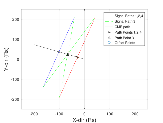
Figure 11: The trajectory of the CME (black line), and the offset point locations relative to this trajectory (open circles). Line 1 (blue), Line 2 (solid green), Line 3 (dashed green), and Line 4 (red) are shown. The locations of the simulated in-situ fits are shown by black triangles.

Each LOS provided a unique measure of the CME. These are summarized in Table 2. With its trajectory offset from the Earth-Sun line by 78 and 102 degrees, the LOS between S/C 1& 4 and 2& 3 provided different measures of the CME structure with Line 2 having less mixing of the sheath and flux rope core. Lines 1 & 4 measured the evolution of the CME structures.

As far as the Faraday rotation simulations are concerned, the normalized Faraday rotation, rotation measure (RM) was calculated for each LOS at each time that a simulation solution was calculated. Note that the time sequence to the solutions was at a higher resolution initially for Line 4 and then more coarse time steps were taken to enable a lengthy recovery phase for analysis. In Future Work, the time steps will be every 100 seconds for more detailed analyses.

When we compared the simple technique for calculating the parallel magnetic field $B_{p}\approx\Delta\chi/TEC\times f_{0}^{2}/A$ to the actual average parallel magnetic field, Panel 3R in Figures 15, 16, 17, and 18 show that these were off by roughly a factor of 2. Closer analysis showed that the discrepancies developed in regions of heightened density. Figure 12 shows how the difference in $B_{p}$ developed over the LOS for a single point in time. This suggests that a tomographic analysis of the TEC could improve the measurement of the average magnetic field in the LOS.

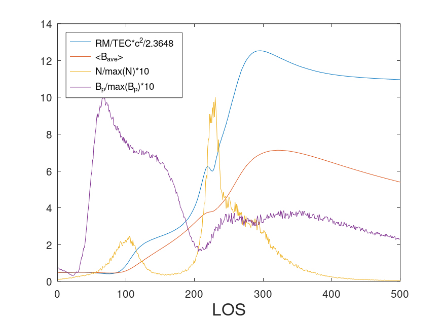
Figure 12: Comparison of the average parallel magnetic field as calculated from FR & TEC (blue line) versus the model’s solution (red line) at a point of time on Line 4. The density and parallel magnetic field along the LOS are plotted, normalized to 10. When the density regionally increases, the differences between the two $B_{p}$ averages increases.

As this paper is concerned with the capabilities and challenges to the FETCH deployment, it is useful to note that in general the approximation of $RM/TEC$ is approximately a factor of 2 off without any further analysis. This is modified in regions of enhanced density such as CME sheath regions, where it can be off by a factor of 5.

The next step in CME analysis is to measure its speed. In order to measure velocity, an average was calculated using the offset points in each line of sight shown in Figure 11 and the arrival time of the leading edge. The velocities in the average were calculated between Lines 1-2, 1-3, 1-4, 2-3, 2-4, and 3-4. This came to be 637.35 km/s. As discussed previously, the AWSoM model speed is around 600 km/s. With the measurement of time and speed, we can begin to estimate the size of the flux rope. In Future Work, we will discuss how FF observations can be used to obtain the perpendicular velocity across each LOS as shown in Panels 1R in Figures 15, 16, 17, and 18.

Measuring the time of the CME crossing requires determining the Leading-Edge (LE) and Trailing-Edge (TE) to the magnetic flux rope. In FETCH data, measuring the group velocity of a signal is potentially too difficult. The phase velocity in contrast affects the observed signal frequency as discussed previously. The Leading-Edge is located in close vicinity to the sheath, or in the case of LOS observations, within it on the descending TEC side. This is visible in the expected FF observations shown in Figure 13. As shown in Table 1, the LE times correspond closely between this technique and the in-situ analysis of simulated Sun-Earth spacecraft data.

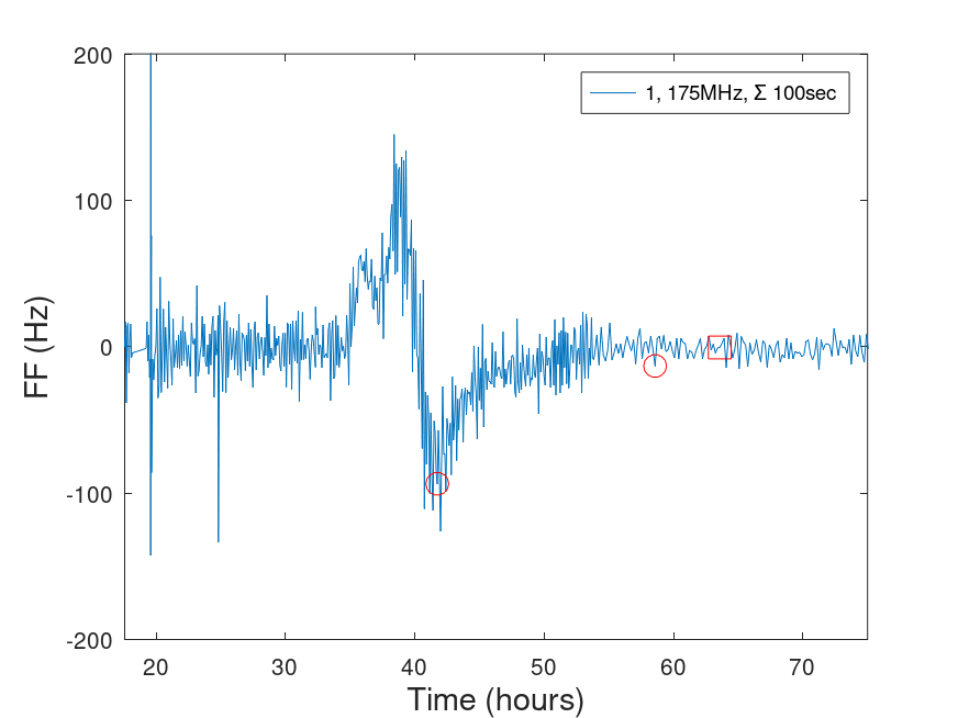
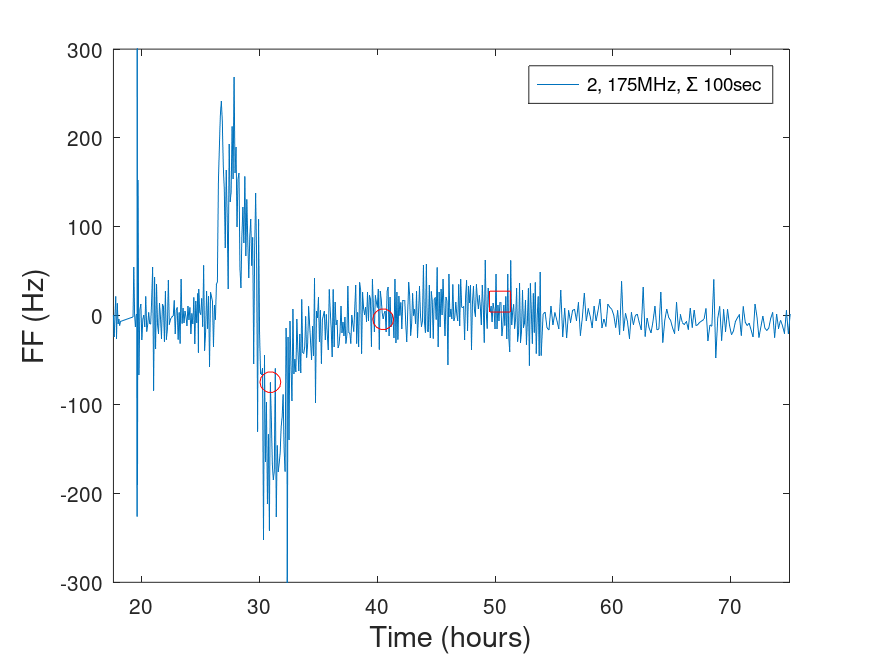
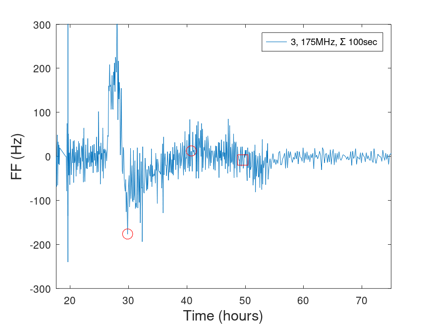
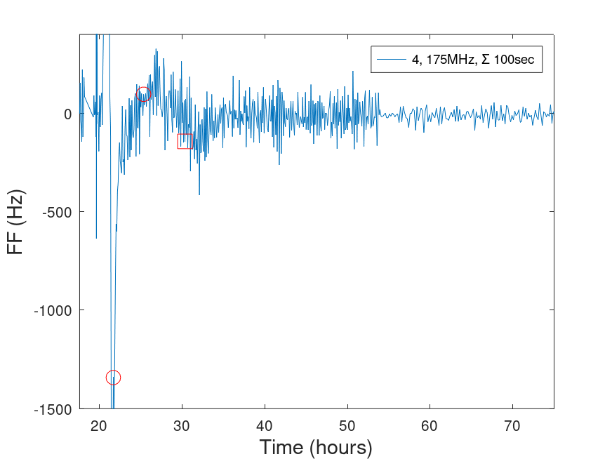
Figure 13: At 175MHz and 100 second integrations, the expected FF response. Circles show the placement of the LE and TE from regions of significant FF change, the minimum and when they turn positive. The square shows the placement of the TE based on in-situ simulation data analysis. A third possible TE placement is where the variability significantly drops.

An issue arises with identifying the TE of the flux rope. There are 3 potential possibilities looking at the FF data as well as the white-light shown in Figure 14. The challenge is to distinguish between them. With the expected available data, 9 other instrument suites, RM, TEC, and FF, one potential approach is to survey the situation and select the solution that is unique to the conditions of the CME’s propagation. As discussed previously, the 2005 CME was a prominence eruption, so there should be some dense material within the flux rope. This eliminates the earliest TE option. Locating the TE from among the center and last option requires further consideration. They all occur right after the extremum in the RM shown in Figures 15, 16, 17, and 18. While this may be appropriate to this case, in order to determine whether this strategy is successful is to consider other cases. This is Future Work. Another approach would be to obtain tomographic solutions for the density; this is also Future Work.

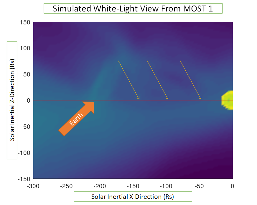
Figure 14: Simulated white-light view from MOST1 or MOST2. The arrows show potential Trailing-Edge solutions. The center one is the one that corresponds to the in-situ TE location.

Line	Leading Edge	Trailing Edge
1	14/17:44 v 14/19:17	15/03:24 v 15/15:27
2	14/06:54 v 14/07:27	14/11:59 v 15/02:17
3	14/05:49 v 14/07:27	14/14:34 v 15/01:27
4	13/21:39 v 13/21:52	14/00:49 v 14/06:12

Table 1: Times from the FF changes shown in Figure LABEL:fig:selecting versus in-situ plasma characteristics.

With the LE and TE determined, a magnetic flux rope model can be fit. The utility of the Taylor-state flux rope model, the J0 and J1 Bessel function solution for the distribution of magnetic field among axial and torroidal components, was investigated. Being a simple model with few free variables, it is a suitable first test case for this situation. Figure 19 shows the model and how it appears in various orientations. There are two effects to note here relative to the 2005 simulation. The fact that the CME passed across the point-of-closest approach (offset point or impact parameter), the distribution of density across it was uniform from a Taylor state model perspective. This added another ambiguity to the clock angle. As shown in Figure 20, no off-axis motion of the CME eliminated characteristics that could distinguish the clock angle uniquely (after accounting for the handedness-orientation ambiguity).

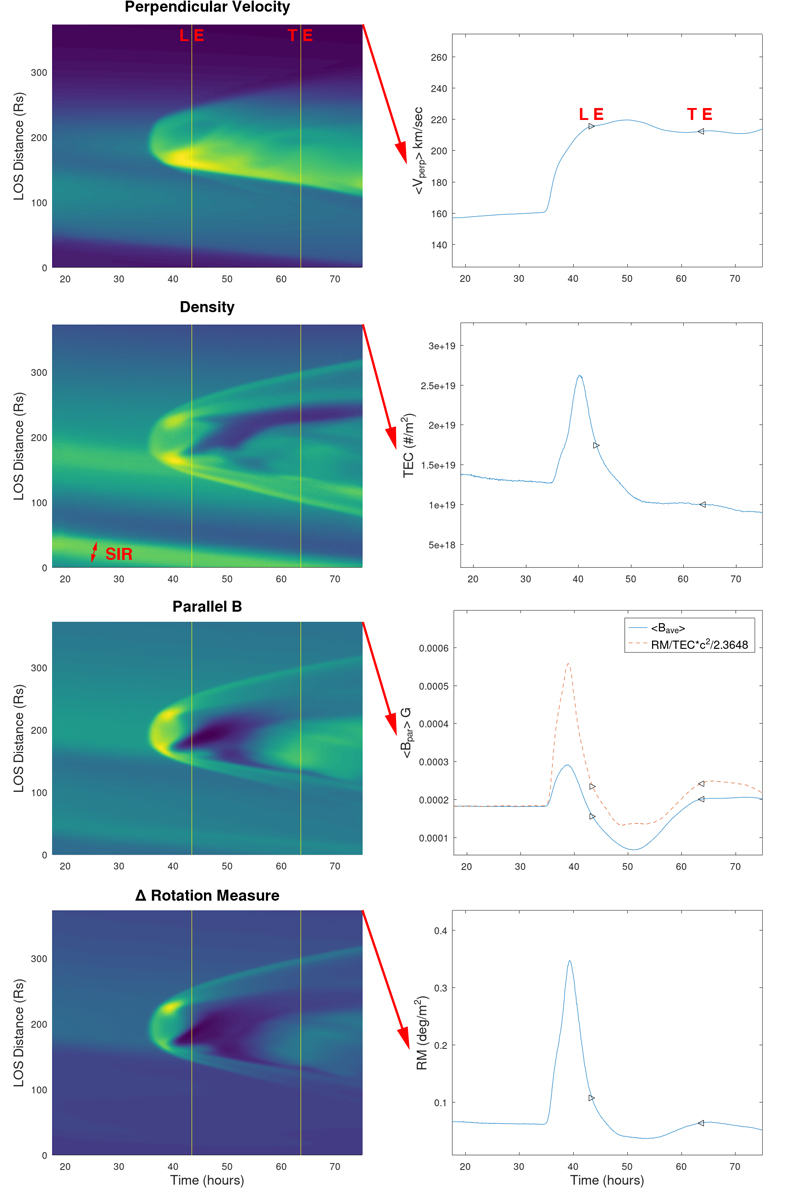
Figure 15: Simulated CME structure extracted along Line 1 Forward (MOST 1$\rightarrow$2) shown in a time series. Shown from top to bottom respectively are the spatial distribution with time of Perpendicular Velocity to the LOS (Panel 1L), the Density (2L, SIR is labeled), the Parallel Magnetic Field to the LOS (3L), and the $\Delta RM$ (4L). The ordinate axis shows the distance along the LOS in solar radii. The plots to the right show the average velocity (1R), the TEC (2R), the average magnetic field (both modeled solid-blue and calculated dashed-red, Panel 3R), and the RM observed at MOST 2 (4R). LE and TE show the Leading and Trailing Edges of the CME from Co-I Nieves-Chincilla’s in-situ analysis.

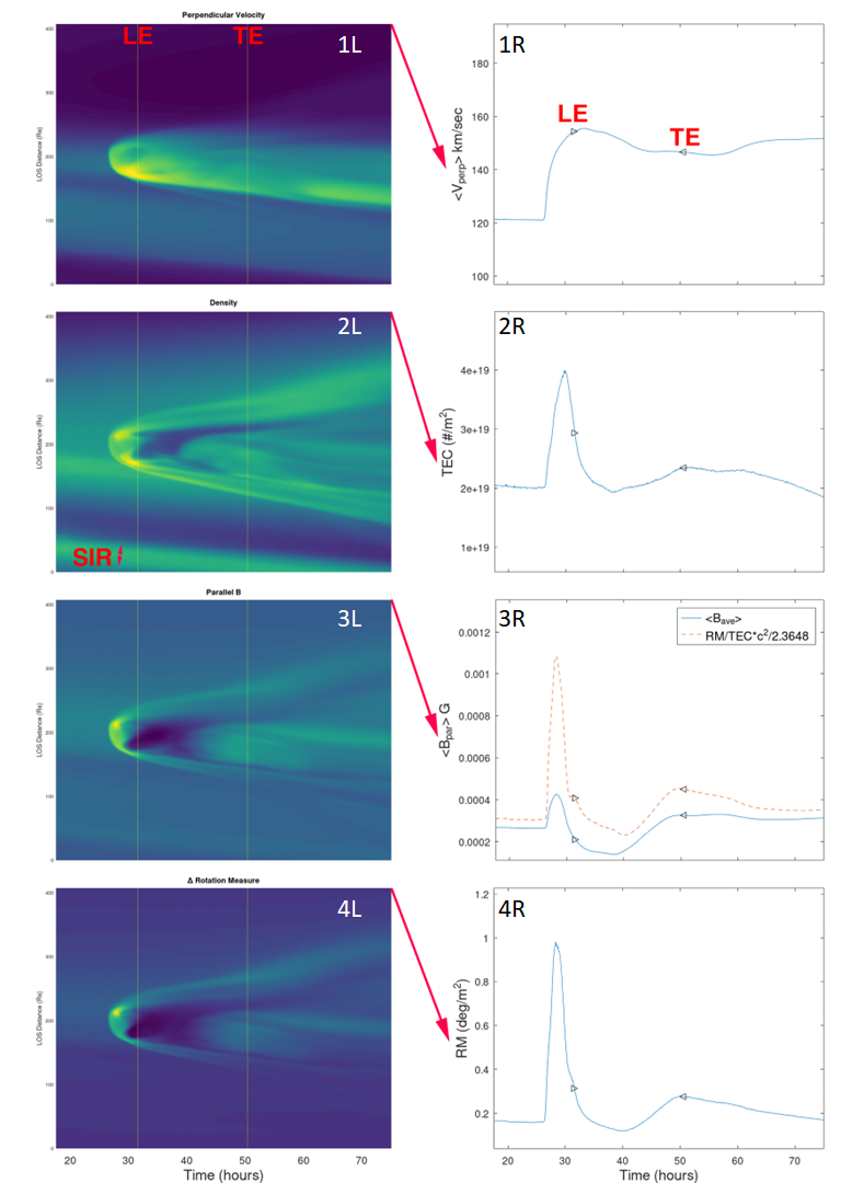
Figure 16: Simulated CME structure extracted along Line 2 Forward (MOST 1$\rightarrow$4) shown in a time series. Shown from top to bottom respectively are the spatial distribution with time of Perpendicular Velocity to the LOS (Panel 1L), the Density (2L, SIR is labeled), the Parallel Magnetic Field to the LOS (3L), and the $\Delta RM$ (4L). The ordinate axis shows the distance along the LOS in solar radii. The plots to the right show the average velocity (1R), the TEC (2R), the average magnetic field (both modeled solid-blue and calculated dashed-red, Panel 3R), and the RM observed at MOST 4 (4R). LE and TE show the Leading and Trailing Edges of the CME from Co-I Nieves-Chincilla’s in-situ analysis.

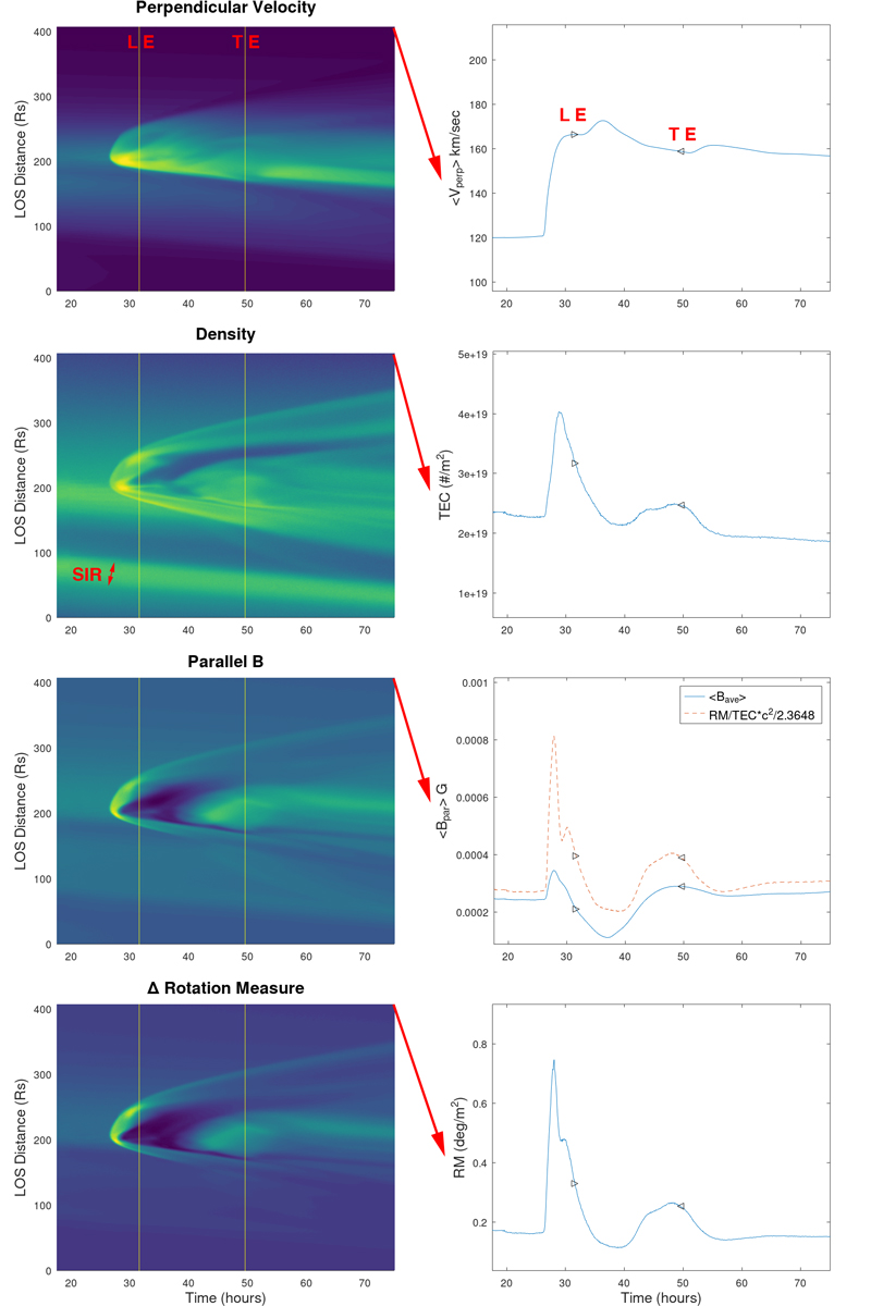
Figure 17: Simulated CME structure extracted along Line 3 Forward (MOST 3$\rightarrow$2) shown in a time series. Shown from top to bottom respectively are the spatial distribution with time of Perpendicular Velocity to the LOS (Panel 1L), the Density (2L, SIR is labeled), the Parallel Magnetic Field to the LOS (3L), and the $\Delta RM$ (4L). The ordinate axis shows the distance along the LOS in solar radii. The plots to the right show the average velocity (1R), the TEC (2R), the average magnetic field (both modeled solid-blue and calculated dashed-red, Panel 3R), and the RM observed at MOST 2 (4R). LE and TE show the Leading and Trailing Edges of the CME from Co-I Nieves-Chincilla’s in-situ analysis.

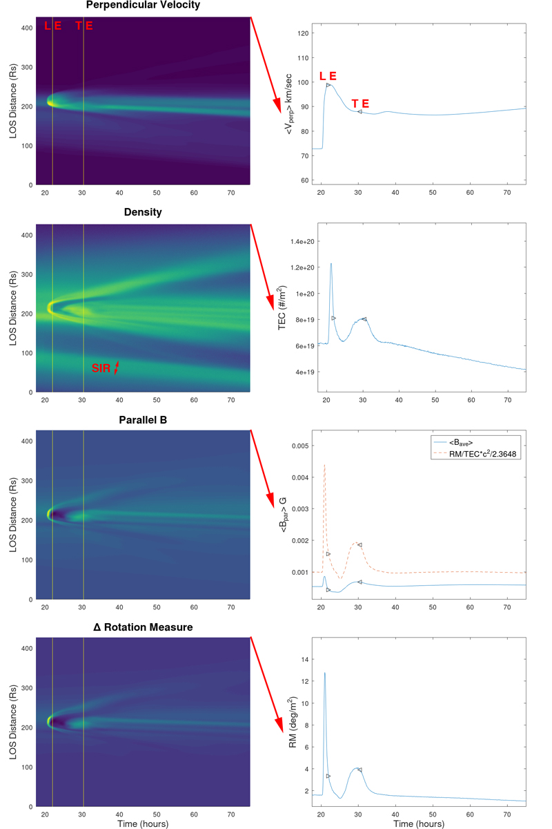
Figure 18: Simulated CME structure extracted along Line 2 Forward (MOST 3$\rightarrow$4) shown in a time series. Shown from top to bottom respectively are the spatial distribution with time of Perpendicular Velocity to the LOS (Panel 1L), the Density (2L, SIR is labeled), the Parallel Magnetic Field to the LOS (3L), and the $\Delta RM$ (4L). The ordinate axis shows the distance along the LOS in solar radii. The plots to the right show the average velocity (1R), the TEC (2R), the average magnetic field (both modeled solid-blue and calculated dashed-red, Panel 3R), and the RM observed at MOST 4 (4R). LE and TE show the Leading and Trailing Edges of the CME from Co-I Nieves-Chincilla’s in-situ analysis.

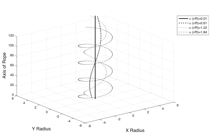
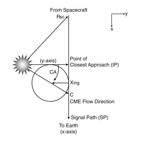
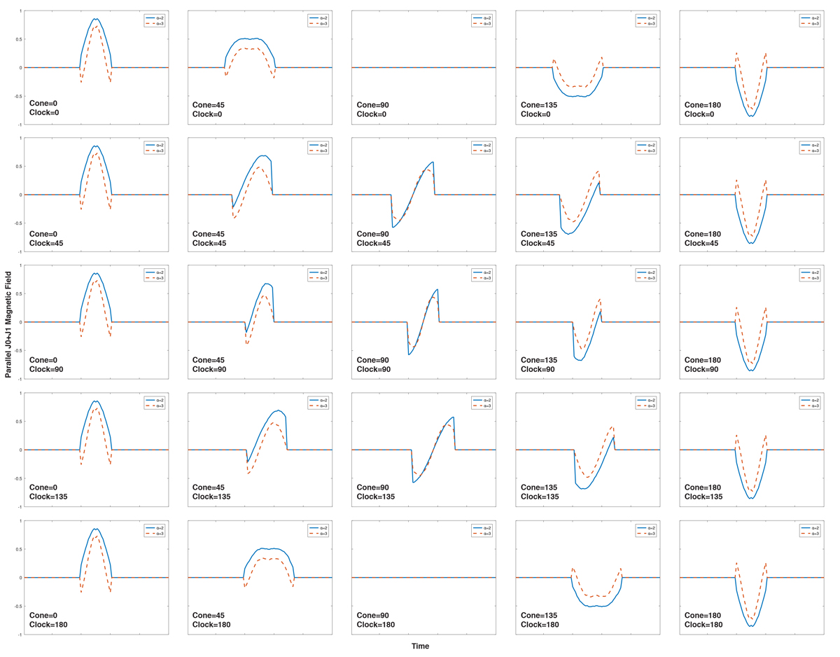
Figure 19: Magnetic flux rope fitting requires a specialized coordinate system to address the unique conditions of Faraday rotation. Taking a force-free flux rope (top left panel, note the $\alpha$ values), it is modeled by crossing a single line-of-sight (top right panel). The clock-cone coordinates are clock: from y-axis (flow direction to IP) to z-axis & cone-complement: from the x-axis. The orientation shown in the example is 90 degree clock and 90 degree cone. The bottom panel shows the parallel magnetic field from various orientations. NOTE: Only for this particular viewing geometry.

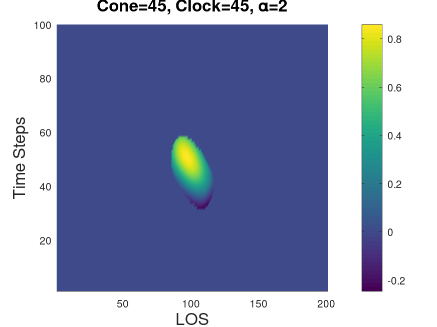
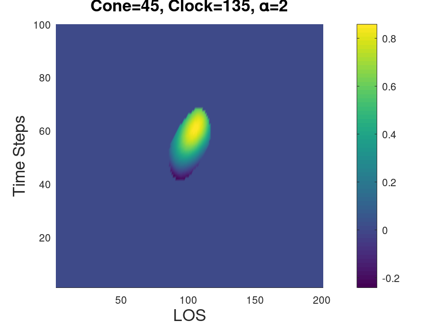
Figure 20: Ambiguity from a lack of off-axis flow. Because the CME is moving in the y-axis direction, no component in the x-axis, two different clock angles will produce the same FR response.

As discussed previously, the average magnetic field is calculated from Faraday rotation using the average TEC measured from the phase time delay and white-light. The force-free Taylor-state flux rope is fit to the average magnetic field using the FF LE and the in-situ TE. The first issue to occur with this was that the LE RM was non-zero in the over-twisted direction. As shown in Figure 19 at 0 and 180 degrees cone angles, over-twisting the Bessel function leads to reversing the direction of the axis on J0. Because this is a situation that does have an in-situ analog, we trimmed the LE to begin where the RM was zero. In order to maintain the location of the center of the flux rope, we also trimmed the TE by the same amount. As shown in Figures 15, 16, 17, and 18, another approach could be to assume the the FR/TEC-calculated magnetic field was too high and should be shift down to zero. The effect of this would be to tilt the axis of the fit down towards the ecliptic.

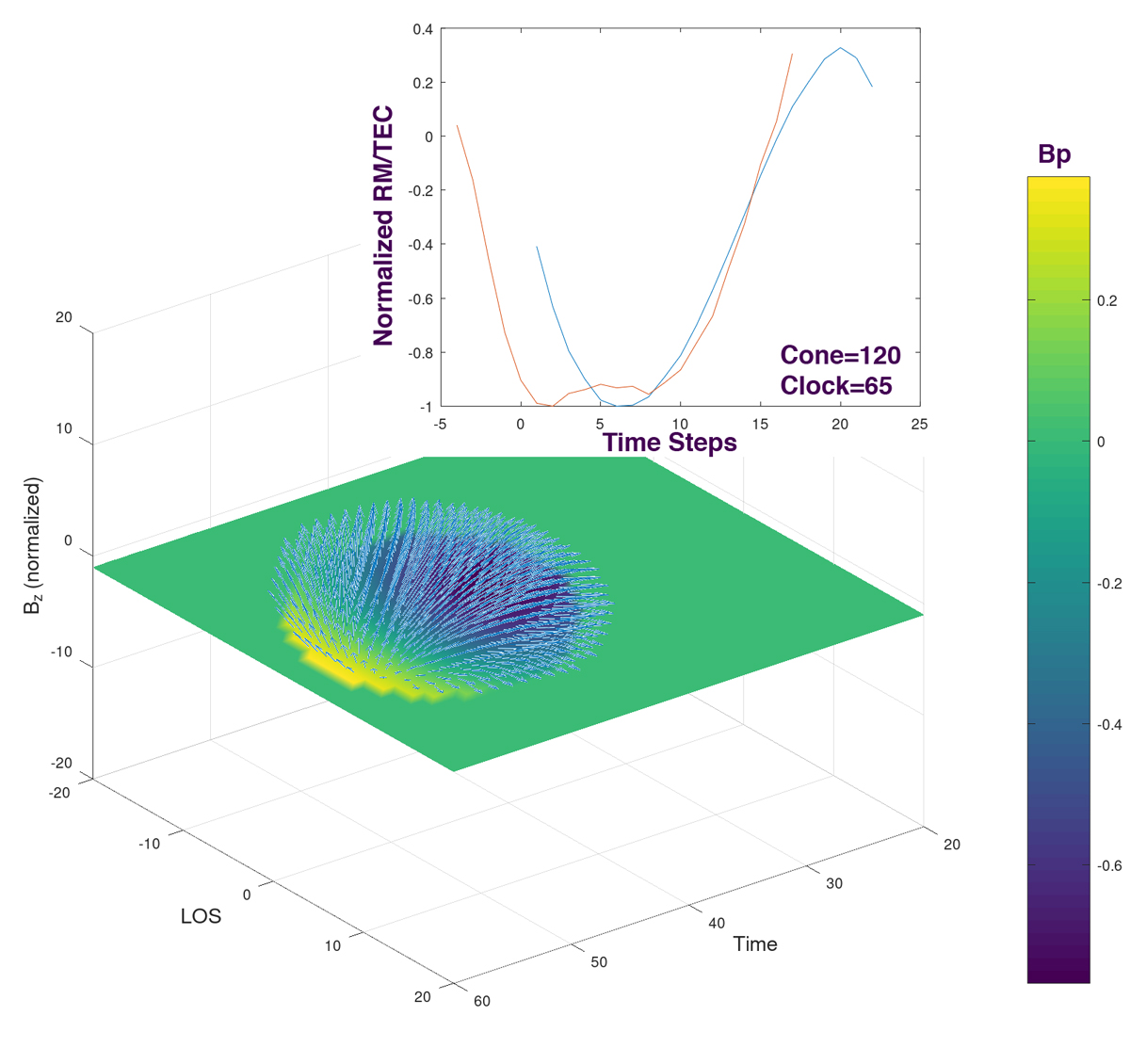
Figure 21: Taylor-state flux rope fit to $B_{p}=RM/TEC*C^{2}/2.3648$ values. The surface plot shows the $\pm B_{p}$ contributing the the fit. The quiver plot shows the direction of the magnetic field vectors from the solution.

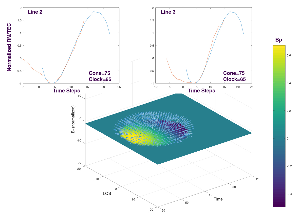
Figure 22: Taylor-state flux rope fit to $B_{p}=RM/TEC*C^{2}/2.3648$ values. The surface plot shows the $\pm B_{p}$ contributing the the fit. The quiver plot shows the direction of the magnetic field vectors from the solution.

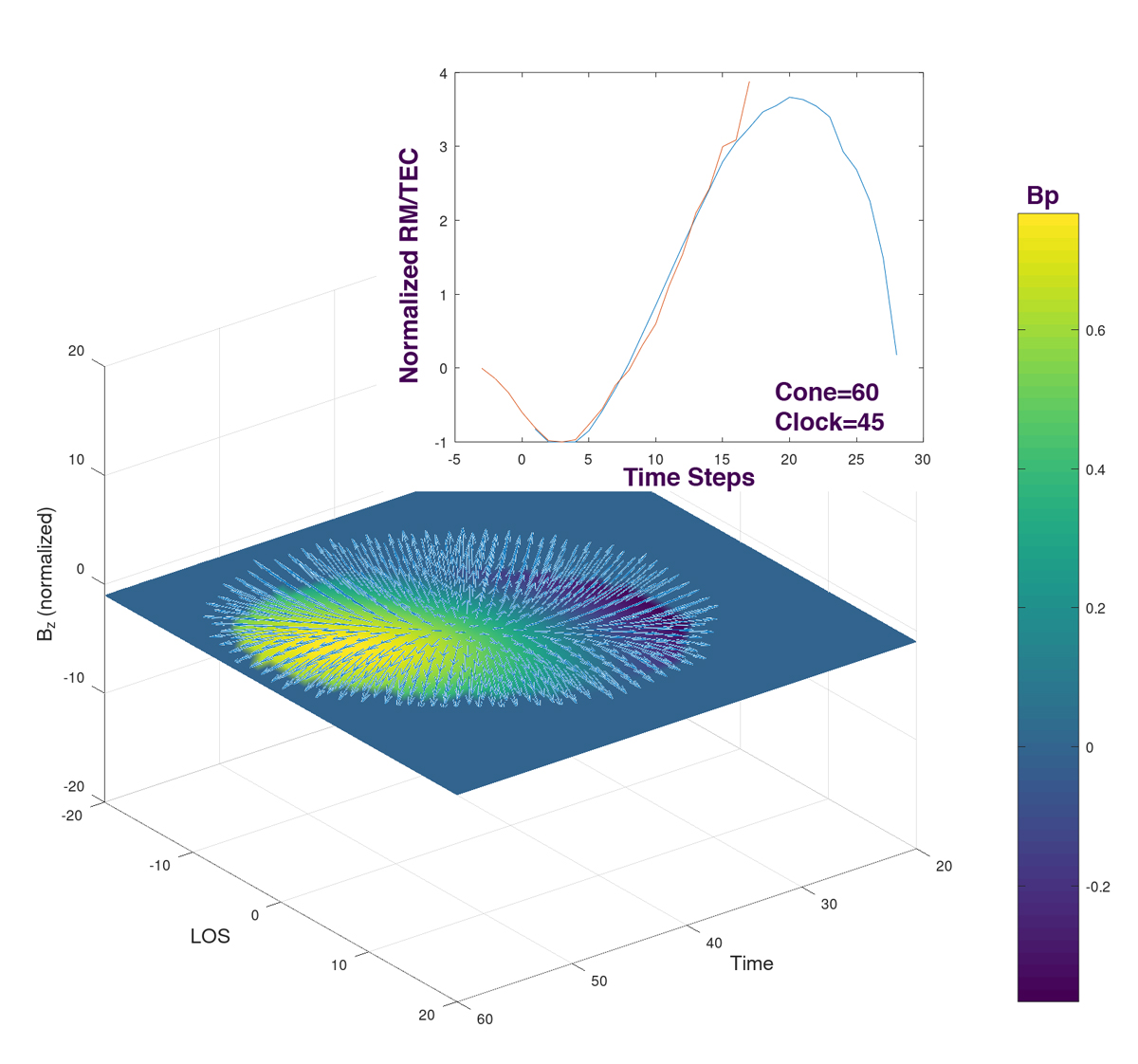
Figure 23: Taylor-state flux rope fit to $B_{p}=RM/TEC*C^{2}/2.3648$ values. The surface plot shows the $\pm B_{p}$ contributing the the fit. The quiver plot shows the direction of the magnetic field vectors from the solution.

The Taylor-state force-free flux rope fits are off-axis by significant amount (Table 2). They do produce a rough estimate of the direction of the flux rope axis (after considering the various degeneracies). Magnetic field magnitude calculations from these fits have been low as shown in the literature (Jensen, 2018; Kooi 2020?). Table 3 shows that while the magnitude is low, the small radius from the fit achieves a reasonable flux comparison between the two approaches. In Future Work, further case studies should be undertaken to see if a scaling factor could be applied to previous research. Other magnetic flux rope models should also be considered to be fit to FR data.

RM Fit (GSE-X, -Y, -Z)	in-situ (GSE-X, -Y, -Z)
$\pm$0.37, -0.5, 0.78	0.01, -0.39, 0.92
$\pm$0.41, 0.26, 0.88	-0.03, -0.10, 0.99
$\pm$0.41, 0.26, 0.88	-0.02, -0.17, 0.99
$\pm$0.61, 0.5, 0.61	-0.14, 0.20, 0.97

Table 2: Comparison of the Right-Handed Orientations of the magnetic flux rope fits. The RM or FR fits were with a Taylor state flux rope model. The in-situ fit were with a MFR model.

RM Fit ($B_{mag}$nT and R AU and flux)	in-situ ($B_{mag}$nT and R AU and flux)
7.7 and 0.085 and 339.24	66.3 and 0.206 and 497.31
16.4 and 0.048 and 2265.7	120.2 and 0.185 and 1117.9
17.0 and 0.054 and 1855.7	121.1 and 0.182 and 1163.7
103.4 and 0.012 and 228,560	612.1 and 0.082 and 28,976

Table 3: Comparison of the axial magnetic field strength, the radius, and the magnetic flux ($B_{mag}/area$ $nT/AU^{2}$) of the magnetic flux rope fits. The RM or FR fits were with a Taylor state flux rope model. The in-situ fit were with a MFR model.

3 Results

This is the first study to analyze Faraday rotation fitting against a high resolution MHD modeled heliosphere. The following results were found:

• The difference between the AWSoM model’s average parallel magnetic field and the one calculated from RM/TEC developed in regions of enhanced density. A tomographic analysis of the TEC could improve the measurement of the average magnetic field in the LOS.

• It is useful to note that in general the approximation of $RM/TEC$ is approximately a factor of 2 off without any further analysis. The error can reach a factor of 5 in regions such as the sheath of the CME.

• The FETCH configuration determined the CME velocity to be 637.35 km/s. As discussed previously, the AWSoM model speed is around 600 km/s.

• In Future Work, we will discuss how FF observations can be used to obtain the perpendicular velocity across each LOS as shown in Panels 1R in Figures 15, 16, 17, and 18.

• As shown in Table 1, the Leading-Edge times correspond closely between the FF technique and the in-situ analysis of simulated Sun-Earth spacecraft data.

• With available information, the Trailing-Edge was determined qualitatively by evaluating the eruption sequence and recognizing that it was near the extremum in RM. While this may be appropriate, other CME cases with the AWSoM model should be examined to confirm this approach. This is Future Work.

• As shown in Figure 20, the FETCH layout for an Earth-propagating CME eliminated the off-axis motion of the CME relative to the LOS closest approach. This eliminated characteristics that could distinguish the clock angle uniquely (after accounting for the handedness-orientation ambiguity). Further CME cases need to be evaluated to determine if this is a significant issue.

• There were other issues with fitting the Taylor-state model. The RM/TEC-calculated magnetic field set the flux rope edge at an extreme alpha number for twist. This could be interpreted as a measure for the magnetic field over-estimation; however, the effect of this would be to tilt the axis of the fit down towards the ecliptic away from the correct orientation.

• Magnetic field magnitude calculations from these fits have been low as shown in the literature. Table 3 shows that while the magnitude is low, the small radius from the fit achieves a reasonable flux comparison between the two approaches.

• Other magnetic flux rope models should also be considered to be fit to FR data.

4 Discussion and Conclusions

Spacecraft radio FR conducted over the L5-L4 sensing path is a novel approach for study of Earth-bound CMEs. Due to the critical magnetic field information extracted by FR methods and the unique orientation of the LOS perpendicular to Earthward-propagating events, the FETCH experiment presents the opportunity to combine the study of CME basic structure and mechanisms with improved early-detection systems for high-risk geospace weather.

The current approach to analyzing the dearth of Faraday rotation observations collected during a CME eruption is to fit a force-free flux rope model to the changes and assume that the magnetic field within the rope is calculated from RM/TEC. This paper demonstrates that the orientation is roughly correct but likely significantly off. While the magnetic field magnitude and size of the flux rope are likely also significantly too small, the magnetic flux through the cross-sectional area from the fit is roughly correct. All of these calculation are impacted by placing the Trailing-Edge of the flux rope, and we propose a qualitative approach to addressing this uncertainty.

Tomographic analysis of Faraday rotation data is likely to improve all of these analyses. The FETCH instrument concept enables this approach.

5 Acknowledgments

E.A. Jensen was supported by ACS Engineering & Safety LLC for this project. Goddard Space Flight Center grant 80NSSC21K1991 supported the software purchases for this work. W. Manchester is supported by the NSF PRE-EVENTS grant No. 1663800 and the NSF SWQU grant No. PHY-2027555. High-performance computing support for this simulations was provided by the NSF/NCAR Yellowstone supercomputer. Basic research at the U.S. Naval Research Laboratory (NRL) is supported by 6.1 Base funding.

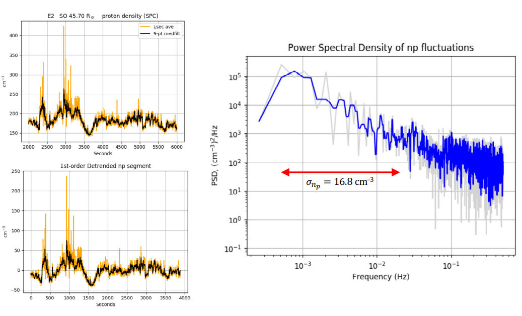
Figure 24: Calculation of the RMS proton density fluctuations. The upper left panel shows the proton number density detected by SWEAP SPC on 2019 April 1 during PSP’s second perihelion encounter (E2) at a solar offset of $45.7\,\mathrm{R}_{\odot}$. The orange and black data are the 1-sec averaged and 9-point median-filtered data, respectively. The lower left panel shows the same data, detrended using a linear fit. The right panel shows the power spectral density, $PSD$, of the proton density fluctuations. The blue and gray data correspond to the 1-sec averaged and 9-point median-filtered data, respectively. Using a frequency range of $0.5-20\,\mathrm{mHz}$, the blue data yield an RMS fractional fluctuation of $\epsilon=0.086$.

To develop an estimate for the variation in plasma density resulting from plasma density fluctuations, we examined data from the Solar Wind Electrons Alphas and Protons (SWEAP Kasper et al., 2016) Solar Probe Cup (SPC) on board the Parker Solar Probe (PSP), corresponding to PSP’s second perihelion encounter. We sampled data from 2019 April 1; although the full data set is available, e.g., in Figure 4 of Rouillard et al. (2020). The sample data set is 4000 sec ($\gtrsim 1\,\mathrm{hr}$), with the proton plasma density, $n_{\mathrm{p}}$, averaged to a one-second cadence (upper left panel of 24). We chose this data because the solar offset was $45.7\,\mathrm{R}_{\odot}$, which is representative of the distances probed by the LOS between S/C 1 and 4 and between S/C 2 and 3.

We detrend the data using a linear fit, resulting in fluctuations about the zero-line (lower left panel of 24). We then determine the power spectral density ($PSD$, right panel of 24); the low frequency limit is determined by the data record length ($1/4000\,\mathrm{sec}=0.25\,\mathrm{mHz}$) and the high frequency limit is set by the Nyquist frequency corresponding to the data sampling rate ($0.5\times 1/1\,\mathrm{sec}=500\,\mathrm{mHz}$). The power spectral density of $n_{\mathrm{p}}$ fluctuations exhibits a negative power scaling ($\alpha\approx-1.6$) from $1-20\,\mathrm{mHz}$ similar to the Kolmogorov spectrum ($\alpha\approx-5/3$) expected for MHD turbulence in the inertial regime. At high frequencies, a noise floor is reached at $\approx 114\,(\mathrm{cm}^{-3})^{2}\,\mathrm{Hz}^{-1}$.

After subtracting the noise floor, the fluctuation variance can be determined by

$$\sigma_{n_{\mathrm{p}}}^{2}=\int_{\nu_{l}}^{\nu_{h}}PSD(\nu)\mathrm{d}\nu$$ (1)

where $\nu_{l}$ and $\nu_{h}$ are the low and high frequency limits, respectively, defining the negative power scaling range (for details of this process, see Wexler et al., 2019). The RMS fluctuations in $n_{\mathrm{p}}$ are then given by $\sigma_{n_{\mathrm{p}}}\equiv\sqrt{\sigma_{n_{\mathrm{p}}}^{2}}$. Over the range $0.5-20\,\mathrm{mHz}$, the RMS fluctuations for this sample is $\sigma_{n_{\mathrm{p}}}=16.8\,\mathrm{cm}^{-3}$. Dividing by the mean density over this sample, $n_{\mathrm{p}}=182.5\,\mathrm{cm}^{-3}$, we obtain a fractional fluctuation of $\epsilon\equiv\sigma_{n_{\mathrm{p}}}/n_{\mathrm{p}}=0.086$.

We also computed the fractional fluctuation $\epsilon$ for the fourth PSP perihelion encounter over a range in data record lengths. For an outer scale of 2400 sec (0.4 mHz frequency limit), $\epsilon=0.07$; for a larger outer scale of 10800 sec (0.1 mHz frequency limit), $\epsilon=0.10$. For comparison, Wexler et al. (2019) estimated $\epsilon=0.08$ at $\approx 10\,\mathrm{R}_{\odot}$ using transcoronal radio data. Similarly, Krupar et al. (2020) found $\epsilon=0.06-0.07$ in PSP data from perihelion encounters 1 and 2 at a temporal scale of 300 seconds. Note, however, much higher fractions may be expected in localized regions during transient solar wind phenomena.

References

- Burlaga (1994) Burlaga, L. F. 1994, J. Geophys. Res., 99, 4161
- Eyles et al. (2003) Eyles, C. J., Simnett, G. M., Cooke, M. P., et al. 2003, Sol. Phys., 217, 319
- Fung et al. (2022) Fung, S. F., Benson, R. F., Galkin, I. A., et al. 2022, in Understanding the Space Environment through Global Measurements, ed. Y. Colado-Vega, D. Gallagher, H. Frey, & S. Wing (Elsevier), 101–216. https://www.sciencedirect.com/science/article/pii/B9780128206300000064
- Gibson & Low (1998) Gibson, S., & Low, B. C. 1998, Astrophys. J., 493, 460
- Howard et al. (2008) Howard, R. A., Moses, J. D., Vourlidas, A., et al. 2008, Space Sci.Rev., 136, 67
- Howard et al. (2016) Howard, T. A., Stovall, K., Dowell, J., Taylor, G. B., & White, S. M. 2016, Astrophys. J., 831, 208
- Hundhausen (1993) Hundhausen, A. J. 1993, J. Geophys. Res., 98, 13177
- Ingleby et al. (2007) Ingleby, L. D., Spangler, S. R., & Whiting, C. A. 2007, Astrophys. J., 668, 520
- Jackson et al. (2006) Jackson, B., Buffington, A., Hick, P., & Webb, D. 2006, JGR, 111, A04S91
- Jackson et al. (2004) Jackson, B. V., Buffington, A., Hick, P. P., et al. 2004, Sol. Phys., 225, 177
- Jensen & Russell (2008) Jensen, E. A., & Russell, C. T. 2008, Geophys. Res. Lett., 35, L02103
- Jensen et al. (2018) Jensen, E. A., Heiles, C., Wexler, D., et al. 2018, Astrophys. J., 861, 118
- Kasper et al. (2016) Kasper, J. C., Abiad, R., Austin, G., et al. 2016, Space Sci. Rev., 204, 131
- Kooi et al. (2021) Kooi, J. E., Ascione, M. L., Reyes-Rosa, L. V., Rier, S. K., & Ashas, M. 2021, Solar Phys., 296, 11
- Kooi et al. (2017) Kooi, J. E., Fischer, P. D., Buffo, J. J., & Spangler, S. R. 2017, Solar Phys., 292, 56
- Kooi et al. (2022) Kooi, J. E., Wexler, D. B., Jensen, E. A., et al. 2022, Frontiers in Astronomy and Space Sciences, 9, 841866
- Krupar et al. (2020) Krupar, V., Szabo, A., Maksimovic, M., et al. 2020, ApJS, 246, 57
- Levy et al. (1969) Levy, G. S., Sato, T., Seidel, B. L., et al. 1969, Science, 166, 596
- Lipiec & Humphreys (2020) Lipiec, E., & Humphreys, B. E. 2020, Space Weather: An Overview of Policy and Select U.S. Government Roles and Responsibilities, Tech. Rep. R46049, Congressional Research Service
- Liu et al. (2007) Liu, Y., Manchester, W. B., I., Kasper, J. C., Richardson, J. D., & Belcher, J. W. 2007, ApJ, 665, 1439
- Manchester et al. (2017) Manchester, W., Kilpua, E. K. J., Liu, Y. D., et al. 2017, Space Sci. Rev., 212, 1159
- Manchester IV et al. (2004) Manchester IV, W., Gombosi, T., Ridley, A., et al. 2004, J. Geophys. Res., 109, doi:10.1029/2003JA010150
- Manchester IV et al. (2014) Manchester IV, W. B., van der Holst, B., & Lavraud, B. 2014, Plasma Phys. Control Fusion, 56, 1
- Manchester IV et al. (2012) Manchester IV, W. B., van der Holst, B., Tóth, G., & Gombosi, T. I. 2012, Astrophys. J., 756, doi:10.1088/0004-637X/756/1/81
- Manchester IV et al. (2005) Manchester IV, W. B., Gombosi, T. I., De Zeeuw, D. L., et al. 2005, Astrophys. J., 622, 1225
- Meng et al. (2015) Meng, X., van der Holst, B., Tóth, G., & Gombosi, T. I. 2015, MNRAS, 454, 3697
- Nieves-Chinchilla et al. (2022) Nieves-Chinchilla, T., Alzate, N., Cremades, H., et al. 2022, ApJ, 930, 88
- Oran et al. (2015) Oran, R., Landi, E., van der Holst, B., et al. 2015, Astrophys. J., 806, 55
- Pätzold & Bird (1998) Pätzold, M., & Bird, M. K. 1998, Geophys. Res. Lett., 25, 2105
- Richardson & Cane (2010) Richardson, I. G., & Cane, H. V. 2010, J. Geophys. Res., 115, 7103
- Riley et al. (2004) Riley, P., Linker, J. A., Mikic, Z., & Odstrcil, D. 2004, IEEE Trans. Plasma Sci., 32, 1415
- Rouillard et al. (2020) Rouillard, A. P., Kouloumvakos, A., Vourlidas, A., et al. 2020, ApJS, 246, 37
- Sachdeva et al. (2019) Sachdeva, N., van der Holst, B., Manchester, W. B., et al. 2019, ApJ, 887, 83
- Sachdeva et al. (2021) Sachdeva, N., Tóth, G., Manchester, W. B., et al. 2021, ApJ, 923, 176
- Sokolov et al. (2013) Sokolov, I. V., van der Holst, B., Oran, R., et al. 2013, Astrophys. J., 764, 23
- Spangler & Whiting (2009) Spangler, S. R., & Whiting, C. A. 2009, in IAU Symp., ed. N. Gopalswamy & D. F. Webb, Vol. 257, 529
- van der Holst et al. (2010) van der Holst, B., Manchester IV, W. B., Frazin, R., et al. 2010, Astrophys. J., 725, 1373
- van der Holst et al. (2014) van der Holst, B., Sokolov, I., Meng, X., et al. 2014, Astrophys. J., 782, 81
- Wexler et al. (2019) Wexler, D. B., Hollweg, J. V., Efimov, A. I., et al. 2019, ApJ, 871, 202
- Woo (1997) Woo, R. 1997, Geophys. Res. Lett., 24, 97
- Wood et al. (2020) Wood, B. E., Tun-Beltran, S., Kooi, J. E., Polisensky, E. J., & Nieves-Chinchilla, T. 2020, Astrophys. J., 896, 99