The Branes Behind
Generalized Symmetry Operators

Abstract

The modern approach to $m$-form global symmetries in a $d$-dimensional quantum field theory (QFT) entails specifying dimension $d-m-1$ topological generalized symmetry operators which non-trivially link with $m$-dimensional defect operators. In QFTs engineered via string constructions on a non-compact geometry $X$, these defects descend from branes wrapped on non-compact cycles which extend from a localized source / singularity to the boundary $\partial X$. The generalized symmetry operators which link with these defects arise from magnetic dual branes wrapped on cycles in $\partial X$. This provides a systematic way to read off various properties of such topological operators, including their worldvolume topological field theories, and the resulting fusion rules. We illustrate these general features in the context of 6D superconformal field theories, where we use the F-theory realization of these theories to read off the worldvolume theory on the generalized symmetry operators. Defects of dimension 3 which are charged under a suitable 3-form symmetry detect a non-invertible fusion rule for these operators. We also sketch how similar considerations hold for related systems.

1 Introduction

One of the important recent advances in the study of quantum field theory (QFT) has been the appreciation that generalized symmetries can often be better understood in terms of corresponding topological operators [1]. For a $d$-dimensional QFT, an $m$-form symmetry naturally acts on $m$-dimensional defects. There is a corresponding dimension $d-m-1$ generalized symmetry operator which is topological, i.e., it is unchanged by local perturbations to its shape [1, 2, 3, 4, 5]. This includes higher-form symmetries, their entwinement via higher-groups, as well as more general categorical structures. One of the general aims in this direction is to use such topological structures to gain access to non-perturbative information on various QFTs. This is especially important in the context of strongly coupled systems where one typically does not have access to a practically useful Lagrangian description of the system.

In this vein, one of the lessons from recent work in stringy realizations of QFT is that there are large families of QFTs which do not have a (known) Lagrangian description. This includes, for example, all 6D superconformal field theories (SCFTs), as well as many compactifications of these theories. More broadly, one can consider the QFT limit of any string background $X$, as obtained by decoupling gravity. In this context, it is natural to expect that the extra-dimensional geometry directly encodes these generalized symmetries.

This expectation is, to a large extent, borne out by the explicit construction of the defect operators of these systems. In the stringy setting, we can generate defects, i.e., non-dynamical objects with formally infinite tension by wrapping branes on non-compact cycles of $X$. The resulting higher symmetries act on these objects, but can be partially screened by dynamical degrees of freedom wrapped on compact cycles of the geometry. This generalized screening argument à la ’t Hooft was used in [6] to define the “defect group” of a 6D SCFT. As noted in [15, 20, 19], specifying a polarization of the defect group amounts to determining the electric / magnetic higher-form symmetries of the system. This perspective has by now been generalized in a number of directions, and has reached the stage where there are explicit algorithms for reading off generalized symmetries for a large number of geometries [6, 20, 23, 34, 29, 26, 25, 42, 46, 128, 53, 63, 70, 129, 72, 76, 130, 77, 78, 94].

One of the puzzling features of these analyses is that the topological operators of reference [1] are in some sense only implicitly referenced in such stringy constructions. The absence of an explicit brane realization of these symmetry topological operators makes it challenging to access some features of generalized symmetries in these systems. For example, it is well-known in various weakly coupled examples that generalized symmetry operators can support a topological field theory, and that in the context of theories with non-invertible symmetries, these can also produce a non-trivial fusion algebra.

In this note we present a general prescription for how to construct topological operators in the context of geometric engineering. We mainly focus on the tractable case of 2-form symmetries for 6D SCFTs and their compactification, as engineered via F-theory backgrounds. In these cases, the generalized symmetry operators arise from D3-branes wrapped on boundary torsional cycles. We find that when the $SL(2,\mathbb{Z})$ bundle of the F-theory model is non-trivial, these models generically have a non-invertible symmetry simply because the fusion algebra for the generalized symmetry operators contains multiple summands. This is quite analogous to what has been observed in the context of various field theoretic constructions [14, 38, 131, 43, 44, 55, 128, 132, 133, 56, 62, 134, 135, 136, 64, 65, 74, 80, 81, 137, 85, 82, 84, 87, 138, 139, 140, 96, 141, 99, 98, 102, 142, 143] as well as some recent holographic models [100, 101].

We emphasize, however, that the construction we present can be applied to essentially any QFT which can be engineered via a string / M- / F-theory compactification. We expect that experts may already be aware of various aspects of this construction, but as far as we are aware, the closest analog of our construction only appeared a few weeks ago in the context of some specific holographic constructions [100, 101].

2 Branes and Generalized Symmetry Operators

Our interest will be in understanding the brane realization of generalized symmetry operators. To frame the discussion to follow, let us first briefly recall how defects are engineered in such systems. We begin by considering a QFT engineered via a string / M-theory background of the form $\mathbb{R}^{d-1,1}\times X$ where $X$ is taken to be a non-compact $D$-dimensional geometry ($d+D=10$ for a string background and $d+D=11$ for an M-theory background). We get a QFT by introducing branes and / or localized singularities at a common point of $X$. These singularities need not be isolated, and can in principle extend all the way out to the boundary $\partial X$. Gravity is decoupled because $X$ is non-compact. This provides a general template for engineering a wide range of (typically supersymmetric) QFTs.

We obtain supersymmetric defects by wrapping BPS branes on non-compact cycles of $X$ which extend from the localized singularity out to the boundary. As explained in [6, 15, 19, 20] a screening argument à la ’t Hooft then tells us that there is a corresponding set of unscreened defects:

$$\mathbb{D=}\underset{m}{\mathbb{{\displaystyle\bigoplus}}}\mathbb{D}^{(m)}\text{ \ \ with \ \ }\mathbb{D}^{(m)}=\underset{p-k=m-1}{{\displaystyle\bigoplus}}\frac{H_{k}(X,\partial X)}{H_{k}(X)},$$ (2.1)

where in the above, the superscript $m$ references an $m$-dimensional defect acted on by an $m$-form symmetry, we sum over supersymmetric $p$-branes and $k$ is a cycle dimension. Specifying a polarization of $\mathbb{D}$ picks an electric / magnetic basis of operators and also dictates the higher-form symmetries via the Pontryagin dual. In the $d$-dimensional QFT, a $p$-brane wrapped on a $k$-cycle will fill out $p+1-k$ spacetime dimensions. We indicate this by saying that the brane fills the space:

$$\widetilde{S}_{p+1}=\widetilde{M}_{p+1-k}\times\widetilde{\Sigma}_{k}=\widetilde{M}_{m}\times\widetilde{\Sigma}_{k},$$ (2.2)

where $\widetilde{\Sigma}_{k}=\mathrm{Cone}(\widetilde{\gamma}_{k-1})$ is the cone generated by extending the boundary cycle $\widetilde{\gamma}_{k-1}\in H_{k-1}(\partial X)$ from infinity to the tip of the cone. A final comment is that the torsional factors of $\mathbb{D}^{(m)}$ will define discrete higher-form symmetries. Non-torsional generators instead label continuous symmetries.

In the $d$-dimensional QFT, the appearance of an $m=(p+1-k)$-dimensional defect implicitly means there are also corresponding operators $\mathcal{O}_{m}$ with support on an $m$-dimensional subspace. The $m$-form symmetry acts on the defects and operators by passing these operators through a topological operator $\mathcal{U}(M_{n})$ with support on an $n$-dimensional subspace. To link with the defect, we have:

$$m+n=d-1.$$ (2.3)

In seeking out an extra-dimensional origin for these operators, we first observe that the defect embeds in spacetime, and extends along the radial direction which starts at the tip of the singularity and goes all the way to the boundary $\partial X$, wrapping a boundary cycle of $H_{k-1}(\partial X)$, namely it is specified by an element of $H_{k}(X,\partial X)$. Our general proposal is that the topological operator which links with this object is given by a magnetic dual brane which links with the original brane in both $X$ as well as the spacetime $\mathbb{R}^{d-1,1}$. In particular, we can wrap a $q$-brane on a cycle of the form:

$$S_{q+1}=M_{q+1-(D-1-k)}\times\gamma_{D-1-k}=M_{n}\times\gamma_{D-1-k},$$ (2.4)

where $\gamma_{D-1-k}$ is a cycle in $H_{D-1-k}(\partial X)$ and $M_{q+1-(D-1-k)}$ is a subspace of the $d$-dimensional spacetime. Observe that in $X$, the cycle does not fill the “radial direction”. Rather, it always “sits at infinity”. Now, for this to be a topological operator which properly links with the defect, we also require:

$$(p+1-k)+(q+1-(D-1-k))=d-1,$$ (2.5)

or equivalently:

$$p+q=D+d-4.$$ (2.6)

But observe that this is just the requirement that in the full string / M-theory background, our sought after $q$-brane is simply the magnetic dual $p$-brane! See figure 1 for a depiction.

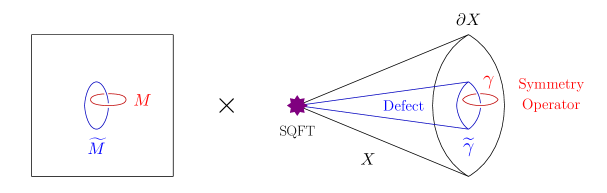
Figure 1: Depiction of a generalized symmetry operator realized via a wrapped brane. We consider a supersymmetric QFT (SQFT) localized at the tip of a conical geometry $X$. At the boundary $\partial X$, we have bounding cycles $\widetilde{\gamma}$ and $\gamma$ which link in $\partial X$. Wrapping a $p$-brane on the cone over $\widetilde{\gamma}$ yields a defect for an $m$-form symmetry, and wrapping the magnetic dual $q$-brane on a linking cycle $\gamma$ realizes a generalized symmetry operator. The spacetime loci $\widetilde{M}$ of the $p$-brane and $M$ of the $q$-brane also link with each other. The wrapped $q$-brane is automatically topological since it sits at infinity in the radial geometry.

We now argue that wrapping a $q$-brane on the cycle at infinity $S_{q+1}=M_{q+1-(D-1-k)}\times\gamma_{D-1-k}$ can be viewed as inserting a topological operator for the $m$-form symmetry. Along these lines, recall that for a (supersymmetric) $p$-brane, there is a corresponding $(p+1)$-form potential $\widetilde{C}_{p+1}$ which couples to this object, and thus a $(p+2)$-form field strength $\widetilde{F}_{p+2}$. In the full higher-dimensional geometry, we also can speak of the dual field strength $\ast\widetilde{F}_{p+2}=F_{q+2}$, as sourced by a magnetic dual $(q+1)$-form potential $C_{q+1}$. The presence of a $p$-brane signals that there is a modified Bianchi identity:

$$dF_{q+2}=\delta_{\widetilde{S}_{p+1}},$$ (2.7)

namely a delta function supported contribution to the flux. Of course, this is just indicating that we have a suitable symmetry current which couples to the magnetic dual potential $C_{q+1}$. Following the general reasoning in [1], we conclude that we can represent our topological symmetry operator by exponentiating the integral of $F_{q+2}$ over the $(q+2)$-chain $Z_{q+2}=M_{q+1-(D-1-k)}\times\mathrm{Cone}(\gamma_{D-1-k})$:

$$\mathcal{U}(Z)=\exp\left(2\pi i\int_{Z}F_{q+2}\right).$$ (2.8)

In particular, if we wish to know the action of $\mathcal{U}(Z)$ on any correlation function, we can simply insert it into the path integral of the $(D+d)$-dimensional supergravity theory.

On the other hand, since we are integrating $F_{q+2}$ over a chain, we can reduce this to the integral of $C_{q+1}$ over the bounding geometry $S_{q+1}=M_{q+1-(D-1-k)}\times\gamma_{D-1-k}$. Since this is an insertion in the path integral, we can view this is as just specifying a “brane at infinity”, namely a $(q+1)$-brane wrapped on the prescribed cycle. Indeed, integrating $C_{q+1}$ over this cycle is just one of the worldvolume couplings of the $q$-brane action. Note also that by wrapping the $q$-brane on a linking cycle at infinity, it is automatically topological from the perspective of the $d$-dimensional QFT. Indeed, any localized fluctuation of such a brane is completely decoupled from the dynamics of the field theory localized at the singularity. The only remaining structure which could in principle persist is purely topological in nature.

Summarizing, our proposal is that for a wrapped $p$-brane which produces a defect, the corresponding generalized symmetry operators which act on these defects are realized by magnetic dual $q$-branes wrapped on linking cycles of the geometry. This is compatible with the holographic discussion considered a few weeks ago in [100, 101], which considers the case of QFTs engineered via D3-brane probes of appropriate singularities. In that setting, the near horizon geometry is of the form $AdS_{5}\times Y$ where $Y$ can be viewed as the asymptotic geometry $\partial X=Y$ probed by the D3-brane. Indeed, as noted in [101], defects arise from branes which fill the radial direction of the $AdS_{5}$, while the symmetry operators arise from branes wrapped on a cycle of $Y$ and sitting at a point of the conformal boundary $\partial AdS_{5}$. It is important to emphasize that precisely because we are dealing with a conformal boundary the construction presented in the holographic setting is indeed compatible with the perspective developed here.

Observe that we can also read off the corresponding topological field theory (TFT) localized on this symmetry operator. Starting from $S_{q+1}=M_{q+1-(D-1-k)}\times\gamma_{D-1-k}$, we consider the topological couplings on the worldvolume theory of our $q$-brane. Roughly speaking, we can integrate this theory along $\gamma_{D-1-k}$ and arrive at a TFT on $M_{n}=M_{q+1-(D-1-k)}$. To see this procedure through from start to finish, then, we need to know the topological couplings on the original brane, as well as a technique to dimensionally reduce along $\gamma_{D-1-k}$.

As a further abstraction, now that we have a method for realizing generalized symmetry operators, we can in principle just consider branes wrapped on torsional cycles “at infinity”. In particular, there is a priori no need for there to exist explicit defects of the appropriate codimension which link with these branes.

3 Example: 2-Form Symmetries of 6D SCFTs

To illustrate the above considerations, we now show how this works in practice for (discrete) 2-form symmetries of 6D SCFTs. All known 6D SCFTs can be engineered via F-theory on an elliptically fibered Calabi-Yau threefold with base $\mathcal{B}$ such that the threefold has a canonical singularity [109, 110, 107]. In the SCFT limit, all of the bases take the form $\mathcal{B}=\mathbb{C}^{2}/\Gamma$ for $\Gamma$ an appropriate finite subgroup of $U(2)$ (see [109] for the classification of all such $\Gamma$). The defect group for the 2-form symmetry is $\mathrm{Ab}[\Gamma]$, the abelianization of $\Gamma$ (see reference [6]). Some basic features of these orbifold singularities are summarized in table 1.

$\Gamma$	$\mathbb{D}^{(2)}$	$L_{\Gamma}$
$\mathbb{Z}_{N}$	$\mathbb{Z}_{N}$	$1/N$
$D_{2N}$	$\mathbb{Z}_{2}\times\mathbb{Z}_{2}$	$\frac{1}{2}\begin{pmatrix}N&N-1\\ N-1&N\end{pmatrix}$
$D_{2N+1}$	$\mathbb{Z}_{4}$	$\frac{2N-1}{4}$
$2T$	$\mathbb{Z}_{3}$	$1/3$
$2O$	$\mathbb{Z}_{2}$	$1/2$
$2I$	1	1
$\mathbb{Z}_{p}(q)$	$\mathbb{Z}_{p}$	$-q/p$
$D_{p+q,q}$	$\begin{array}[]{c}\mathbb{Z}_{2p}\times\mathbb{Z}_{2}~{}\textnormal{($q$ even)}\\ \mathbb{Z}_{2p}~{}\textnormal{($q$ odd)}\end{array}$	(See main text)

Table 1: In the left column we list out all of the families of finite subgroups of $U(2)$ associated to 6D SCFTs. Here $D_{k}$ means the dicyclic groups of order $2k$, and $2T$, $2O$, and $2I$ denote the binary tetrahedral, octahedral, and icosahedral groups respectively. $\mathbb{Z}_{p}(q)$ denotes a $\mathbb{Z}_{p}$ subgroup of $U(2)$ generated by an action $(z_{1},z_{2})\mapsto(\zeta_{p}z_{1},\zeta^{q}_{p}z_{2})$ ($p$ and $q$ coprime). Finally, $D_{p+q,q}$ is a $U(2)$ subgroup which generalizes the dicyclic group (see [109, 6] and references therein for more details).

It is helpful to decompose the base geometry as a fibration $S^{3}/\Gamma\rightarrow\mathcal{B}\rightarrow\mathbb{R}_{\geq 0}$ in which the SCFT sits at the point $r=0$ in $\mathbb{R}_{\geq 0}$ where the $S^{3}/\Gamma$ collapses to zero size. We can introduce a defect by wrapping a D3-brane on the radial direction of $\mathbb{R}_{\geq 0}$ as well as a torsional 1-cycle of $S^{3}/\Gamma$. In this case, we expect the topological operator which acts on such defects to be given by a D3-brane which wraps the boundary torsional 1-cycle as well as a three-dimensional subspace $M_{3}$ of the 6D spacetime.

The procedure for how to work out the TFT generated by our wrapped D3-brane follows similar steps to those developed in [101]. Starting from the D3-brane worldvolume theory, we have the topological couplings [145, 146]:

$$\mathcal{S}_{\text{top}}^{D3}=2\pi i\int_{S}\exp(\mathcal{F}_{2})\sqrt{\frac{\widehat{A}(TS)}{\widehat{A}(NS)}}\left(C_{0}+C_{2}+C_{4}\right),$$ (3.1)

where here, $\mathcal{F}_{2}=F_{2}-B_{2}$, with $F_{2}$ the $U(1)$ gauge field strength of the D3-brane, and $B_{2}$ the (pullback of) the NS-NS 2-form potential. Additionally, the $C_{m}$ are the pullbacks of RR potentials onto the worldvolume of the D3-brane. Due to $SL(2,\mathbb{Z})$ duality covariance, we will label the 2-form curvatures as $F_{3}:=dB_{2}$ and $F^{D}_{3}:=dC_{2}$. Expanding out, the relevant couplings for us are, expressed in differential cohomology (see e.g., [147, 70]),:

$$\mathcal{S}_{\text{top}}^{D3}=2\pi i\int_{S}\breve{F}_{5}+\breve{F}^{D}_{3}\star\mathcal{\breve{F}}_{2}+\breve{F}_{1}\star\left(\frac{1}{2}\mathcal{\breve{F}}_{2}\star\mathcal{\breve{F}}_{2}+\frac{1}{24}\breve{e}\right),$$ (3.2)

with $\breve{e}$ the Euler class of $S$. Comparing with [101], it will turn out to be important to also track the term involving $\breve{F}_{1}\star\mathcal{\breve{F}}_{2}\star\mathcal{\breve{F}}_{2}$. On the other hand, the contribution from the Euler term will play little role in the present analysis.

One might ask how a term involving $F_{1}$ arises from purely field theoretic considerations. Indeed, because there are no continuous marginal parameters in 6D SCFTs [150, 151], one might be tempted to conclude that no such dependence could be present. Observe, however, that the 6D SCFT admits 4D defects (i.e., codimension two defects) given by D3-brane probes of the local model. The worldvolume of this D3-brane contains a continuous parameter $\tau$ which is precisely what is also entering in our generalized symmetry operators.

To proceed further, we need to dimensionally reduce the WZ terms of the D3-brane wrapped on a torsional cycle $\gamma$ of the extra-dimensional geometry. There is a subtlety here in cases where the $SL(2,\mathbb{Z})$ bundle of an F-theory model is non-trivial because these duality transformations act on the axio-dilaton as well as the doublet of 2-form potentials of the IIB background. Consequently, the first case we consider involves the 6D SCFTs with $\mathcal{N}=(2,0)$ supersymmetry. In these cases the elliptic fibration is completely trivial, which simplifies the analysis of the D3-brane topological terms. We next treat the case of single curve non-Higgsable cluster theories [152]. In this case, the presence of a non-trivial duality bundle leads us to a discrete Chern-Simons gauge theory on the generalized symmetry operator, which potentially coupled to background fields. We expect similar considerations to hold in any background where the axio-dilaton is constant. In all these cases, we find that 3D defects charged under a suitable 3-form symmetry detect a non-invertible symmetry, namely the fusion algebra for the symmetry operators contains multiple summands.

The most general situation in which the axio-dilaton is position dependent is, by the same reasoning, expected to also lead to non-invertible symmetries. We anticipate that more general possibilities can arise once we consider topological operators which are also fused with those associated with the 0-form and 1-form symmetries of these 6D SCFTs. These generically arise once we take into account the contributions from flavor 7-branes (see e.g., [130, 77, 94]).

Though we leave the details for future work, it is also clear that we can apply the same methodology when we compactify a 6D SCFT on a background manifold $Q$ of dimension $l$. Indeed, all that is required is that we also wrap the topological operator on the relevant cycle (possibly torsional) of $Q$, and again perform the appropriate dimensional reduction.

3.1 6D $\mathcal{N}=(2,0)$ Theories

As a first class of examples, consider the 6D $\mathcal{N}=(2,0)$ SCFTs as engineered by type IIB on an ADE singularity $\mathbb{C}^{2}/\Gamma$ with $\Gamma$ a finite subgroup of $SU(2)$. We begin by considering the case $\Gamma$ a cyclic group and then turn to the case of $\Gamma$ non-abelian.

$\Gamma$ Cyclic

Consider first the case where $\Gamma$ is a cyclic group. The topological field theory of the operator constructed from the D3-brane is then derived by reduction in differential cohomology on the quotient $S^{3}/\Gamma$. Let us denote the cohomology generators of $S^{3}/\Gamma$ by $1,u_{2},\textnormal{vol}$ in degree 0,2,3 and their lift to differential cohomology by $\breve{1},\breve{u}_{2},\textnormal{\u{v}ol}$. We expand as

$$\breve{F}_{5} =\breve{a}_{2}*\textnormal{\u{v}ol}+\breve{a}_{3}*\breve{u}_{2}+\breve{a}_{5}*\breve{1}$$ (3.3)

$$\breve{F}_{3} =\breve{b}_{0}*\textnormal{\u{v}ol}+\breve{b}_{1}*\breve{u}_{2}+\breve{b}_{3}*\breve{1}$$

$$\breve{F}_{2} =\breve{c}_{0}*\breve{u}_{2}+\breve{c}_{2}*\breve{1}$$

$$\breve{F}_{1} =\breve{d}_{1}*\breve{1}$$

and similarly for $\breve{F}_{2}^{D},\breve{F}_{3}^{D}$, where the “D” superscript refers to the field strength obtained under an S-duality transformation. The coefficients multiplying $\breve{u}$ are background fields for the discrete symmetries

$$\breve{a}_{3}\leftrightarrow\mathbb{Z}_{N}^{(2)}\,,\qquad\breve{b}_{1}\leftrightarrow\mathbb{Z}_{N}^{(0)}\,,\qquad\breve{c}_{0}\leftrightarrow\mathbb{Z}_{N}^{(-1)}\,,$$ (3.4)

while those multiplying $\breve{1}$ are field strengths for the continuous abelian symmetries

$$\breve{b}_{3}\leftrightarrow U(1)^{(1)}\,,\qquad\breve{c}_{2}\leftrightarrow U(1)^{(0)}\,,\qquad\breve{d}_{1}\leftrightarrow U(1)^{(-1)}$$ (3.5)

In the above, the superscripts $(s)$ refer to the corresponding $s$-form symmetry. The expansion along v̆ol is a standard reduction and as $S^{3}/\Gamma$ has formally infinite volume $\breve{a}_{2},\breve{b}_{0}$ are non-dynamical, measuring fluxes which are absent in the purely geometric background (and therefore vanish). The self-duality of $\breve{F}_{5}$ implies the vanishing of $\breve{a}_{5}$. Regarding the axio-dilaton, the curvature of $\breve{d}_{1}$ is identified with $R(\breve{d}_{1})=d(\mathrm{Re}(\tau))\in H_{1}(M_{3},\mathbb{Z})$ and when this class is trivial, then the data contained in the differential cohomology class $\breve{d}_{1}$ is simply $\tau$. With this in mind, we will also employ a slight redefinition of the $\breve{F}_{3}$ fields to get rid of the cumbersome $\tau$ factors in the D3 topological action which is $F^{new}_{3}\equiv\frac{1}{\tau}F^{old}_{3}$ and $(F^{D})^{new}_{3}\equiv\tau(F^{D}_{3})^{old}$. Consistency with Dirac quantization follows from lifting these fields to M-theory on a torus fibration in the standard duality dictionary, i.e., we interpret the type IIB $SL(2,\mathbb{Z})$ covariant 3-form flux as an M-theory 4-form flux reduced on the elliptic fiber.

We emphasize now that in this case there is no flux non-commutativity contrary to the setup in [15]. To see why, consider the Hamiltonian formulation by writing $M_{3}=N_{2}\times\mathbb{R}_{t}$. We get the pair of electric and magnetic flux operator valued in the $\text{Tor}\,H^{2}(N_{2}\times\gamma;\mathbb{Z})$ as $\Phi_{e}(b_{0}\star u_{2})$ and $\Phi_{m}(c_{0}\star u_{2})$. Now on $N_{2}$, the Poincaré duals $PD[b_{0}]$ and $PD[c_{0}]$ do not intersect for degree reasons, so $\Phi_{e}(b_{0}\star u_{2})$ commutes with $\Phi_{m}(c_{0}\star u_{2})$ and there are no terms involving co-boundaries giving rise to non-commutativity upon quantization as in [101] that describes a discrete gauge theory in the sense of [154].

We insert the expansion (3.3) into our expression for the topological action to find:

$$\mathcal{S}_{\textnormal{top}}^{\textnormal{D3}}=\frac{2\pi i}{N}\int_{M_{3}}\bigg{(}a_{3}+c_{0}\cup b^{D}_{3}+c_{0}^{D}\cup b_{3}+c_{2}\cup b^{D}_{1}+c_{2}^{D}\cup b_{1}$$ (3.6)

$$-c_{0}\cup b_{3}-c^{D}_{0}\cup b^{D}_{3}-c_{2}\cup b_{1}-c^{D}_{2}\cup b^{D}_{1}\bigg{)},$$

where we have added terms derived from similar expansions for $\breve{F}_{2}^{D}$ to restore invariance under S-duality. Notice that terms coming from expanding $\breve{F}_{3}^{D}$ are already present in the $\frac{1}{2}\breve{F}_{1}\star\mathcal{\breve{F}}_{2}\star\mathcal{\breve{F}}_{2}$ term in (3.2). The above action simplifies after defining linear combinations given by $b_{1}^{\prime}\equiv b^{D}_{1}-b_{1}$, $b_{3}^{\prime}\equiv b^{D}_{3}-b_{3}$, $c_{0}^{\prime}\equiv c_{0}-c^{D}_{0}$, and $c_{2}^{\prime}\equiv c_{2}-c^{D}_{2}$ after which the topological action is just

$$\mathcal{S}_{\textnormal{top}}^{\textnormal{D3}}=\frac{2\pi i}{N}\int_{M_{3}}\left(a_{3}+c^{\prime}_{0}\cup b^{\prime}_{3}+c^{\prime}_{2}\cup b^{\prime}_{1}\right).$$ (3.7)

Recall that $\breve{F}_{2}$ and $\breve{F}_{2}^{D}$ are worldvolume field strengths on the D3-brane at infinity and therefore $c_{0},c_{2}$ and their dual partners are path-integrated over. The topological operator therefore takes the form:

$$\mathcal{U}(M_{3})=\frac{1}{\mathcal{K}}\int Dc^{\prime}_{0}Dc^{\prime}_{2}\exp\left(\mathcal{S}_{\textnormal{top}}^{\textnormal{D3}}\right)$$ (3.8)

where $\mathcal{K}$ is a normalization constant we determine shortly. In our definition of $\mathcal{U}(M_{3})$, we have left implicit the dependence on the torsional 1-cycle of the boundary geometry (to avoid cluttering notation). At this point, unless otherwise stated, we assume that this torsional 1-cycle is a generator of $H_{1}(S^{3}/\Gamma,\mathbb{Z})$. The topological operator $\mathcal{U}(M_{3})$ is a product of the operator

$$\mathcal{U}_{0}=\exp\left(\frac{2\pi i}{N}\int_{M_{3}}a_{3}\right)\,,$$ (3.9)

which is the standard flux operator for surface defects of the SCFT, and

$$\mathcal{U}_{1} =\frac{1}{|H_{1}(M_{3},\mathbb{Z}_{N})|}\int Dc^{\prime}_{2}\exp\left(\frac{2\pi i}{N}\int_{M_{3}}c^{\prime}_{2}\cup b^{\prime}_{1}\right)\,,$$ (3.10)

$$\mathcal{U}_{3} =\frac{1}{N}\int Dc^{\prime}_{0}\exp\left(\frac{2\pi i}{N}\int_{M_{3}}c^{\prime}_{0}\cup b^{\prime}_{3}\right)\,.$$

So altogether we have

$$\mathcal{U}(M_{3})=\mathcal{U}_{0}\mathcal{U}_{1}\mathcal{U}_{3}\,.$$ (3.11)

which sets the normalization constant $\mathcal{K}$. When the $C_{2}$ and $B_{2}$ backgrounds are turned off we have, $\mathcal{U}(M_{3})=\mathcal{U}_{0}$.

Let us now study the fusion algebra. Note that all operators except $\mathcal{U}_{0}$ are condensation operators since they specify a 3-gauging of a $U(1)^{(3)}$ or $\mathbb{Z}^{(4)}_{N}$ symmetry along the $M_{3}$ worldvolume. Moreover, we show that these operators satisfy the fusion algebra of projections

$$\mathcal{U}_{i}\mathcal{U}_{i}=\mathcal{U}_{i}\,,\;\;\;\;\textnormal{($i=1,3$)},$$ (3.12)

and so formally speaking are non-invertible. That being said, they are invertible when restricted to their image where they equate to the identity operator. This follows for instance for $\mathcal{U}_{1}$ by the manipulations

$$\mathcal{U}_{1} =\frac{1}{|H_{1}(M_{3},\mathbb{Z}_{N})|}\int Dc^{\prime}_{2}\exp\left(\frac{2\pi i}{N}\int_{M_{3}}c^{\prime}_{2}\cup b^{\prime}_{1}\right)$$ (3.13)

$$=\frac{1}{|H_{1}(M_{3},\mathbb{Z}_{N})|}\sum_{\ell\in H_{1}(M_{3},\mathbb{Z}_{N})}\exp\left(\frac{2\pi i}{N}\int_{\ell}b^{\prime}_{1}\right)$$

$$=\frac{1}{|H_{1}(M_{3},\mathbb{Z}_{N})|}\prod_{\ell^{\prime}}\left(\sum_{k=0}^{N-1}\exp\left(\frac{2\pi ik}{N}\int_{\ell^{\prime}}b^{\prime}_{1}\right)\right)$$

together with the integrality of the periods of $b^{\prime}_{1}$. Here $\{\ell^{\prime}\}$ are a generating set for the lattice $H_{1}(M_{3},\mathbb{Z}_{N})$. So whenever such periods are non-vanishing we have a vanishing sum of roots of unity. From this we also see that $\mathcal{U}_{i}=\mathcal{U}_{i}^{\dagger}$ for $i\neq 0$ follows from relabeling $k\rightarrow-k$. The normalization is now explicitly $\mathcal{K}=N|H_{1}(M_{3},\mathbb{Z}_{N})|$. On the other hand the operator $\mathcal{U}_{0}$ displays a cyclic fusion ring

$$\mathcal{U}_{0}\mathcal{U}_{0}^{\dagger}=1\,,\qquad\mathcal{U}_{0}^{n}=\exp\left(\frac{2\pi in}{N}\int_{M_{3}}a_{3}\right).$$ (3.14)

Concerning the operators charged under $\mathcal{U}(M_{3})$, these include the surface operators of the defect group $\mathbb{D}$ constructed from D3-branes wrapped on relative 2-cycles of the F-theory base $\mathcal{B}$. The operators $\mathcal{U}_{1},\mathcal{U}_{3}$ do not act on elements of $\mathbb{D}$ since they carry no charge under the symmetries of (3.4) and (3.5) other than $\mathbb{Z}_{N}^{(2)}$. Therefore the restriction of $\mathcal{U}(M_{3})$ on $\mathbb{D}$ is given by $\mathcal{U}_{0}$, namely the standard flux operator. However, as mentioned at the end of Section 2, $\mathcal{U}(M_{3})$ can act on operators with spacetime dimension other than $2$ as well. The $\mathcal{U}_{1}$ piece acts on local operators of the 6D SCFT that originate from $D1$ and $F1$ strings wrapping a torsional 1-cycle in the boundary $S^{3}/\Gamma$ times the radial direction of $\mathbb{C}^{2}/\Gamma$, while the $\mathcal{U}_{3}$ piece acts on line operators that wrap a point in $S^{3}/\Gamma$ times the radial direction. The actions of $\mathcal{U}_{1}$ and $\mathcal{U}_{3}$ on these operators is almost trivial: it multiplies by zero on any operators with non-zero charge under the symmetry groups $\mathbb{Z}^{(0)}_{N}$ and $U(1)^{(1)}$ respectively.

$\Gamma$ Non-Abelian

Consider next the case where $\Gamma$ is non-abelian. As far as the defect group is concerned, the relevant data is captured by the abelianization $\mathrm{Ab}[\Gamma]$. Returning to the entries of Table 1, we see that in nearly all cases, we again have a single cyclic group factor so the analysis proceeds much as we already presented. On the other hand, for some $D$-type subgroups, $\mathrm{Ab}[\Gamma]$ has two cyclic group factors. For this reason, we now focus on this case.

Proceeding more generally, when we insert the above expansion (3.3) into (3.2), the overall coefficient we obtain in the exponential is given by the canonical link pairing in first homology:

$$L_{\Gamma}:\;H_{1}(S^{3}/\Gamma)\times H_{1}(S^{3}/\Gamma)\rightarrow\mathbb{Q}/\mathbb{Z}.$$ (3.15)

This is because given $\breve{t}^{i}_{2}$ such that $I(\breve{t}^{i}_{2})=t^{i}_{2}\in H^{2}(S^{3}/\Gamma,\mathbb{Z})\simeq\mathbb{Z}_{n_{i}}\times\mathbb{Z}_{n_{j}}$ we have that

$$\int_{S^{3}/\Gamma}\breve{t}^{i}_{2}*\breve{t}^{j}_{2}=L^{ij}_{\Gamma}.$$ (3.16)

Table 1 gives the explicit linking pairing for all $\Gamma$ a finite subgroup of $SU(2)$.

Let us turn next to the TFT obtained from wrapping a D3-brane on a torsional cycle of $S^{3}/\Gamma$. When $\breve{H}^{2}(S^{3}/\Gamma)$ has more than one generator, the previously considered $\breve{a}_{3}$, $\breve{b}_{1}$, and $\breve{c}_{0}$ each pick up an index. In determining the spectrum of topological operators, it is enough to consider D3-branes wrapping $\gamma=\nu^{1}\gamma_{1}+\nu^{2}\gamma_{2}$, with $\gamma_{i}$ a primitive generators of $H_{1}(S^{3}/\Gamma)$. The action is now (reverting back to the original duality basis for clarity):

$$\mathcal{S}_{\textnormal{top}}^{\textnormal{D3}}=2\pi\sqrt{-1}\nu^{i}(L_{\Gamma})_{ij}\underset{M_{3}}{\int}\bigg{(}a^{j}_{3}+c^{j}_{0}\cup b^{D}_{3}+(c_{0}^{D})^{j}\cup b_{3}+c_{2}\cup(b_{1}^{D})^{j}+c_{2}^{D}\cup b^{j}_{1}$$ (3.17)

$$-c^{j}_{0}\cup b_{3}-(c_{0}^{D})^{j}\cup b^{D}_{3}-c_{2}\cup b^{j}_{1}-c_{2}^{D}\cup(b_{1}^{D})^{j}\bigg{)}.$$

Just as in the case of $\Gamma=\mathbb{Z}_{N}$, we observe that the fusion rules for these topological operators produce an invertible symmetry when the background $C_{2}$ and $B_{2}$ fields are switched off.

3.2 6D NHC Theories

We now turn to rank one 6D $\mathcal{N}=(1,0)$ theories in which the axio-dilaton is constant but the duality bundle of the F-theory model is still non-trivial. In particular, we consider the case of the single curve non-Higgsable clusters (NHCs) of reference [152] in which the base of the F-theory model supports a curve of self-intersection $-n$ for $n=3,4,6,8,12$. These models can be written as $(\mathbb{C}^{2}\times T^{2})/\mathbb{Z}_{n}$, where the action on the $\mathbb{C}^{2}$ base is by a common $n^{th}$ primitive root of unity [155, 109]. On the tensor branch, these theories are characterized by a 6D gauge theory coupled to a tensor multiplet with charge prescribed by the self-intersection number. With notation as in [109], we have:

$$\overset{\mathfrak{su}(3)}{3},\;\;\overset{\mathfrak{so}(8)}{4},\;\;\overset{\mathfrak{e}_{6}}{6},\;\;\overset{\mathfrak{e}_{7}}{8},\;\;\overset{\mathfrak{e}_{8}}{12}$$ (3.18)

where $\overset{\mathfrak{g}}{n}$ refers to a $(-n)$-curve with a ADE singularity of type $\mathfrak{g}$ wrapping it. These can all be presented as F-theory backgrounds $(\mathbb{C}^{2}\times T^{2})/\mathbb{Z}_{n}$ (see [155, 109]) where the quotient is defined by the group action:

$$(z_{1},z_{2},z_{3})\rightarrow(\zeta_{n}z_{1},\zeta_{n}z_{2},\zeta^{-2}_{n}w)$$ (3.19)

where $w$ is the torus-fiber coordinate. In the nomenclature of table 1, $\Gamma=\mathbb{Z}_{n}{(1)}$ (i.e., $p=n$ and $q=1$), and thus the link pairing is $L_{\Gamma}=1/n$.

To build $\mathcal{U}(M_{3})$, we again wrap a D3 on $M_{3}\times\gamma$ where $\gamma$ is a generating 1-cycle with boundary homology class $\gamma\in H_{1}(S^{3}/\Gamma)$, but now there is a non-trivial $SL(2,\mathbb{Z})$ monodromy for $n=3,\;4,\;6,\;8$ and $12$. This clearly modifies the expansion of $\breve{F}_{3}$, $\breve{F}_{2}$, and their duals in such a way that one must generally consider the vectors $(F_{2},F^{D}_{2}),(F_{3},F^{D}_{3})$ modulo some relations as well-defined objects rather than the individual components. More precisely, we need to expand these fields in cohomology with the twisted coefficient module

$$(\mathbb{Z}\oplus\mathbb{Z})_{\rho}$$ (3.20)

where $\rho$ is the $SL(2,\mathbb{Z})$ monodromy of order $k$ when going around $\gamma$ as given in table 2.

$n$	Kodaira Type	Monodromy $\rho$	$k=\mathrm{ord}(\rho)$	Tor $H_{1}(T_{3})$	$L_{\gamma}^{t}$
3	$IV$	$\left(\begin{array}[]{cc}0&1\\ -1&-1\end{array}\right)$	3	$\mathbb{Z}_{3}$	1/3
4	$I_{0}^{*}$	$\left(\begin{array}[]{cc}-1&0\\ 0&-1\end{array}\right)$	2	$\mathbb{Z}_{2}\oplus\mathbb{Z}_{2}$	$\left(\begin{array}[]{cc}0&1/2\\ 1/2&0\end{array}\right)$
6	$IV^{*}$	$\left(\begin{array}[]{cc}-1&-1\\ 1&0\end{array}\right)$	3	$\mathbb{Z}_{3}$	2/3
8	$III^{*}$	$\left(\begin{array}[]{cc}0&-1\\ 1&0\end{array}\right)$	4	$\mathbb{Z}_{2}$	1/2
12	$II^{*}$	$\left(\begin{array}[]{cc}0&-1\\ 1&1\end{array}\right)$	6	$0$	$0$

Table 2: Topological data for asymptotic geometries of 6D $\mathcal{N}=(1,0)$ SCFTs. The F-theory geometry consists of an elliptic fibration over a Lens space base containing a torsional 1-cycle $\gamma$. The torus fibration restricted to $\gamma$ gives a three-manifold $T_{3}$, a torus bundle more precisely, whose torsion and linking forms $L^{t}_{\gamma}$ we list, see [48]. D3 branes wrapped on $\gamma$ map under M-/F-theory duality to M5-branes wrapped on $T_{3}$.

We begin by computing the twisted cohomology of the boundary of the base space $S^{3}/\Gamma=\partial(\mathbb{C}^{2}/\Gamma)$. Via an identical computation to that given in section 3.2 of [156], we get

$$H^{*}(S^{3}/\mathbb{Z}_{n};(\mathbb{Z}\oplus\mathbb{Z})_{\rho})=\{0,G_{k},0,G_{k}\}$$ (3.22)

where

$$G_{k}=\left\{\begin{array}[]{lll}\mathbb{Z}_{2}\oplus\mathbb{Z}_{2}&\quad k=2&\quad(n=4)\\ \mathbb{Z}_{3}&\quad k=3&\quad(n=3,6)\\ \mathbb{Z}_{2}&\quad k=4&\quad(n=8)\\ 1&\quad k=6&\quad(n=12)\end{array}\right.$$ (3.23)

Now, $\breve{F}_{5}$ associated with D3 branes should be reduced on untwisted differential cocycles $\breve{u}_{i}\in\breve{H}^{i}(S^{3}/\Gamma;\mathbb{Z})$:

$$\breve{F}_{5}=\breve{a}_{2}\star\textnormal{\u{v}ol}+\breve{a}_{3}\star\breve{u}_{2}+\breve{a}_{5}\star\breve{1},\\$$ (3.24)

whereas $\breve{F}_{3},\breve{F}_{3}^{(D)}$ associated with D1 and F1 strings and the worldvolume $\breve{F}_{2},\breve{F}_{2}^{(D)}$ should be reduced on twisted differential cocycles $\breve{t}_{i}\in\breve{H}^{i}(S^{3}/\Gamma;(\mathbb{Z}\oplus\mathbb{Z})_{\rho})$. The reduction goes as follows: when $k\neq 2$ (here $\rho$ in the superscript stands for self-dual operators that are compatible with the $\rho$ twisting):

$$\begin{split}\breve{F}_{3}^{\rho}=\left(\begin{array}[]{c}\breve{F}_{3}\\ \breve{F}_{3}^{(D)}\end{array}\right)/\mathrm{Im}(\rho-1)&=\breve{b}_{2}^{\rho}\star\breve{t}_{1}+\breve{b}_{0}^{\rho}\star\breve{t}_{3}\\ \breve{F}_{2}^{\rho}=\left(\begin{array}[]{c}\breve{F}_{2}\\ \breve{F}_{2}^{(D)}\end{array}\right)/\mathrm{Im}(\rho-1)&=\breve{c}_{1}^{\rho}\star\breve{t}_{1}\,.\end{split}$$ (3.25)

Similar expansions hold for $\breve{b}_{0}^{\rho}$ and $\breve{b}_{2}^{\rho}$. The notation of the lefthand side denotes the reduction of $(\breve{F}_{2},\breve{F}_{2}^{(D)})$ modulo $SL(2,\mathbb{Z})$ monodromy. The fields $c_{n}$ and $b_{m}$ are discrete $G_{k}$ valued $n$-cocycles and $m$-cocycles where $G_{k}=\mathbb{Z}_{2},\mathbb{Z}_{3}$ as in (3.23) respectively.

When $k=2$ we have the decomposition

$$H^{i}(S^{3}/\Gamma;(\mathbb{Z}\oplus\mathbb{Z})_{\rho})=H^{i}(S^{3}/\Gamma;(\mathbb{Z})_{\rho})^{(e)}\oplus H^{i}(S^{3}/\Gamma;(\mathbb{Z})_{\rho})^{(m)}$$ (3.26)

with $\rho=-1$ for each coefficient ring. Consequently the expansion is then

$$\breve{F}_{2}=\breve{c}_{1}\star\breve{t}_{(e),1}\,,\qquad\breve{F}_{2}^{(D)}=\breve{c}_{1}^{D}\star\breve{t}_{(m),1}$$ (3.27)

where $I(\breve{t}_{(e,m),1})=t_{(e,m),1}$ generates $H^{1}(S^{3}/\Gamma;(\mathbb{Z})_{\rho})^{(e,m)}$. Similar expansions hold for $\breve{b}_{0}$ and $\breve{b}_{2}$. In this case all fields are discrete $\mathbb{Z}_{2}$ co-cycles with the degree as indicated by their index.

When reducing the $\breve{F}_{5}$ term, the non-zero term comes from

$$\int_{S^{3}/\Gamma}\breve{u}_{2}\star\breve{u}_{2}\equiv L_{\Gamma}(\breve{u}_{2})$$ (3.28)

on $S^{3}/\Gamma$. This gives the contribution to the action of

$$\exp\left(2\pi iL_{\Gamma}(\breve{u}_{2})\int_{M_{3}}a_{3}\right).$$ (3.29)

For $\breve{F}_{3},\breve{F}_{3}^{(D)},\breve{F}_{2},\breve{F}_{2}^{(D)}$, on the other hand, the non-zero terms can be evaluated from the pairing of the twisted cohomology classes on $\gamma\in H_{1}(S^{3}/\Gamma;\mathbb{Z})$:

$$k=3,4\,: \int_{\gamma}\breve{t}_{1}\star\breve{t}_{1}\equiv L_{\gamma}^{t}(\breve{t}_{1})$$ (3.30)

$$k=2\,: \int_{\gamma}\breve{t}_{(e),1}\star\breve{t}_{(m),1}\equiv L_{\gamma}^{t}(\breve{t}_{(e),1},\breve{t}_{(m),1})$$

which we both denote by $L_{\gamma}^{t}$ whenever the context is clear. The self-pairing of $\breve{t}_{(e,m),1}$ vanishes as we shortly argue.

The pairing between twisted classes in differential cohomology generalizing torsional linking are computed using the methods in reference [157]. M-/F-theory duality gives a natural relation of such pairings to linking forms in ordinary singular homology. We now explain this relation as we perform our computations from the latter perspective.

To frame the discussion we introduce the torus bundle three-manifold $T_{3}$ as the restriction of the S-duality torus bundle to the 1-cycle $\gamma$ wrapped by the D3 brane. As all three-manifolds its homology groups are fully determined by $H_{1}(T_{3};\mathbb{Z})$ which is computed by application of the Mayer-Vietoris sequence to

$$H_{1}(T_{3})=\mathbb{Z}\oplus\textnormal{coker}\,(\rho-1)$$ (3.31)

where $\rho$ is the $SL(2,\mathbb{Z})$ monodromy matrix acting on 1-cycles upon traversing $\gamma$. The torsional subgroups are listed in table 2. The linking form on $T_{3}$ follows from similar considerations [48]. Let us denote the torsional generators of $\textnormal{Tor}\,H^{2}(T_{3};\mathbb{Z})$ by $t_{2}$ which by Poincaré duality and the universal coefficient theorem is dual to the generators $\ell_{1}$ of $\textnormal{Tor}\,H_{1}(T_{3};\mathbb{Z})$. When the monodromy matrix is of type $I_{0}^{*}$ $(k=2)$ both $t_{2}$ and $\ell_{1}$ are further indexed by $(e,m)$ distinguishing the factors in $\textnormal{Tor}\,H_{1}(T_{3};\mathbb{Z})\cong\mathbb{Z}_{2}\oplus\mathbb{Z}_{2}$ for that case.

Now note that M-/F-theory duality maps a D3 brane wrapped on $\gamma\times M_{3}$ to an M5-brane wrapped on $T_{3}\times M_{3}$ where $M_{3}$ is the space-time submanifold supporting the topological operator. The Wess-Zumino-Witten term of the M5-brane contains the term [158, 159]

$$\mathcal{S}_{\text{top}}^{M5}\supset 2\pi i\int_{M_{3}\times T_{3}}\breve{F}_{7}+\frac{1}{2}\breve{F}_{3}\star\breve{F}_{4}$$ (3.32)

where $\breve{F}_{3}$ is the anti-self-dual 3-form field strength (of the anti-chiral 2-form field on the M-theory worldvolume), and $\breve{F}_{7}$ is the pullback of the magnetic dual 7-form field strength. We can therefore equivalently compute the topological field theory on $M_{3}$ starting from the action (3.32). This approach however expresses the coefficient of the topological theory via geometric data of $T_{3}$ and avoids $SL(2,\mathbb{Z})$ twisted cohomology classes. We therefore conjecture that the pairing (3.30) is geometrized to a link pairing on the torus bundle

$$k=3,4\,: L_{\gamma}^{t}(\breve{t}_{1})=\int_{\gamma}\breve{t}_{1}\star\breve{t}_{1}=\int_{T_{3}}\breve{t}_{2}\star\breve{t}_{2}$$ (3.33)

$$k=2\,: L_{\gamma}^{t}(\breve{t}_{(e),1},\breve{t}_{(m),1})=\int_{\gamma}\breve{t}_{(e),1}\star\breve{t}_{(m),1}=\int_{T_{3}}\breve{t}_{(e),2}\star\breve{t}_{(m),2}=\frac{1}{2}$$

where the righthand side is computed by the linking pairing given in table 2. We will have more to say on the M-theory perspective in section 4. Evidence for the identity (3.33) is already given in [101] which considers a setup with $-1\in SL(2;\mathbb{Z})$ monodromy along $\gamma$ and where the case $k=2$ in (3.33) was found to hold.

Before writing down the full topological action of our D3-brane, we must first comment on the expected non-commutativity of flux operators in this scenario. Due to the presence of a non-trivial duality bundle, there is a mixing between the electric and magnetic dynamical two-form curvatures on the D3 worldvolume gauge theory, so considering the on-shell relation $F^{D}_{2}=*F_{2}$ (see for instance [160]) we must quantize these fields as a self-dual Maxwell theory. This is especially clear in the M5-brane picture where the flux quantization is already that of anti-self-dual fields and the torsion homology of the $T^{2}$-bundle precisely descends to the torsion in the twisted homology that the D3-brane wraps. Depending on the value of $k$, it is occasionally possible to have a canonical splitting of electric and magnetic fluxes on the D3.

Now expanding on the treatment of [101] to examine the non-commutativity of fluxes on the D3 worldvolume in our cases, we first assume that $M_{3}=N_{2}\times\mathbb{R}_{t}$ to employ a Hamiltonian formalism. The Hilbert space associated to the spatial manifold $N_{2}\times\gamma$ of the D3-brane worldvolume will then be a representation a Heisenberg algebra, the details of which depend on the value of $k$. The Heisenberg algebra is generated by non-commuting electric and magnetic flux operators $\Phi_{e},\Phi_{m}$ respectively detecting fluxes through torsional cycles. The cases are:

• For $k=2$, we have a pair of non-commuting electric and magnetic fluxes associated with $\mathrm{Tor}\,H^{2}(N_{2}\times\gamma)$:

  $$\Phi_{e}(\breve{c}_{1}\star\breve{t}_{(e),1})\Phi_{m}(\breve{c}_{1}^{(D)}\star\breve{t}_{(m),1})=\exp\left(2\pi iL_{\gamma}^{t}(\breve{t}_{(e),1},\breve{t}_{(m),1})\right)\Phi_{m}(\breve{c}_{1}^{(D)}\star\breve{t}_{(m),1})\Phi_{e}(\breve{c}_{1}\star\breve{t}_{(e),1})$$ (3.34)

  we thus get a $\mathbb{Z}_{2}$ gauge theory as in [147], with the action given by

  $$\mathcal{S}_{\mathbb{Z}_{2}}=\pi i\int_{M_{3}}c_{1}\cup\delta c_{1}^{(D)}$$ (3.35)

  where $(c_{1},c_{1}^{(D)})$ are a pair of discrete gauge fields which together are valued in $G_{2}=\mathbb{Z}_{2}\times\mathbb{Z}_{2}$. In other words, $c_{1}$ and $c_{1}^{(D)}$ are each separately $\mathbb{Z}_{2}$ valued discrete gauge fields normalized such that $\int c_{1}=\ell\;\mathrm{mod}\;2$.

• For $k=3,4,6$, we have a pair of non-commuting self-dual fluxes associated with $\mathrm{Tor}\,H^{2}(N_{2}\times\gamma)$. Now, extra care has to be taken since the electric and magnetic field has to be the same [15]. For $x,y\in H^{1}(\gamma;(\mathbb{Z}\oplus\mathbb{Z})_{\rho})$

  $$\Phi_{a}(\breve{c}_{1}^{\rho}\star\breve{x})\Phi_{b}(\breve{c}_{1}^{\rho}\star\breve{y})=\exp\left(2\pi iL_{\gamma}^{t}(\breve{x},\breve{y})\right)\Phi_{b}(\breve{c}_{1}^{\rho}\star\breve{y})\Phi_{a}(\breve{c}_{1}^{\rho}\star\breve{x})$$ (3.36)

  here $L^{t}_{\gamma}(x,y)$ is the bilinear form of the twisted linking pairing. Thus, we need to include a discrete CS gauge theory of the form

  $$\mathcal{S}=2\pi iL^{t}_{\gamma}(\breve{t}_{1})\int_{M_{3}}c_{1}^{\rho}\cup\delta c_{1}^{\rho},$$ (3.37)

  where $c^{\rho}_{1}$ is a discrete gauge field valued in $G_{k}$ as in (3.23) normalized such that $\int c^{\rho}_{1}=\ell\;\mathrm{mod}\;\mathrm{2\;or\;3}$.

Furthermore, the topological actions generating the link pairing above produce an additional term in the effective action of the D3 brane reduced on the twisted 1-cycle, the middle term(s) in both lines of (3.38), because the effective action must be a functional of the gauge invariant combination $\delta c^{\rho}_{1}-b^{\rho}_{2}$ where $b^{\rho}_{2}$ is defined in the first line of equation (3.25).

To summarize then, we get the action of the topological operator (where again we keep the dependence on the torsional 1-cycle implicit, include a normalization factor $\mathcal{K}^{-1}$, and leave the cup products implicit) $\mathcal{U}(M_{3})=\mathcal{K}^{-1}\exp(\mathcal{S}_{\textnormal{top}}^{\textnormal{D3}})$ as:

$$k=2 :\qquad\mathcal{S}_{\textnormal{top}}^{\textnormal{D3}}=2\pi i\int_{M_{3}}\bigg{(}-\tfrac{1}{4}a_{3}-\tfrac{1}{2}b^{(D)}_{2}c_{1}-\tfrac{1}{2}b_{2}c_{1}^{(D)}+\tfrac{1}{2}c_{1}\delta c_{1}^{(D)}\bigg{)}$$ (3.38)

$$k=3,4,6 :\qquad\mathcal{S}_{\textnormal{top}}^{\textnormal{D3}}=2\pi i\int_{M_{3}}\bigg{(}L_{\Gamma}a_{3}-L_{\gamma}^{t}b_{2}^{\rho}c_{1}^{\rho}+L_{\gamma}^{t}c_{1}^{\rho}\delta c_{1}^{\rho}\bigg{)}$$

where for $k=3,4,6$, the path integral is written as $\mathcal{K}^{-1}\int Dc_{1}^{\rho}\exp\left(\mathcal{S}_{\textnormal{top}}^{\textnormal{D3}}\right)$ with the implicit understanding that a delta–function relating $c_{1},c_{1}^{(D)}$ has been inserted to gauge fix the monodromy relations of line (3.25). For the values of both $L_{\Gamma}=L_{\Gamma}(\breve{u}_{2})=\frac{1}{n}$ and $L_{\gamma}^{t}=L_{\gamma}^{t}(\breve{t}_{1})$ see table 2. Also, in this subsection the normalization factor will be $\mathcal{K}=(|H_{2}(M_{3},G_{k})|)^{1/2}$ for reasons that will be clear in what follows.

Notice that due to the coupling to the various $b_{2}$ fields in line (3.38), we see again, just as in subsection 3.1, that the symmetry operator $\mathcal{U}(M_{3})$ acts on more than just dimension-2 operators in the defect group $\mathbb{D}$. The $b_{2}$’s are background fields for a discrete $G_{k}^{(1)}$-symmetry and are sourced by defects constructed from $(p,q)$-5-branes wrapping homology classes in $H_{2}(S^{3}/\Gamma,(\mathbb{Z}\oplus\mathbb{Z})_{\rho})=\mathrm{Hom}(G_{k},U(1))$ times the radial direction of $\mathbb{C}^{2}/\Gamma$.

Notice that due to the presence of terms like $c\delta c$ in (3.38), we see that even if we ignore terms involving $b_{2}$ fields (and hence the effect of $\mathcal{U}(M_{3})$ on the line operators mentioned in the previous paragraph) our 2-form symmetry operators are tensored with discrete topological gauge theories, namely some level-N Dijkgraaf-Witten theories with gauge group $G_{k}$, $\mathcal{T}^{(N,G_{k})}$. The levels of these gauge theories are classified by by $H^{4}(G_{k},\mathbb{Z})$ [162], and the possible levels relevant to single node NHCs are $H^{4}(\mathbb{Z}_{N},\mathbb{Z})=\mathbb{Z}_{N}$ and $H^{4}(\mathbb{Z}^{2}_{2},\mathbb{Z})=\mathbb{Z}^{3}_{2}$. Our action (3.38) thus predicts the levels of these discrete gauge theories living on the defect group symmetry operators and notice that the operator fusion simply adds together the cyclically defined Chern-Simons levels, so this confirms that that $\mathcal{U}(M_{3})$ appears to be an invertible operator when linking with operators with trivial charge under the $G^{(1)}_{k}$ symmetry.

Fusion Rules We now turn to the fusion rules for our symmetry operators, namely we compute $\mathcal{U}(M_{3})\times\mathcal{U}^{\dagger}(M_{3})$. We find that in the presence of the $G^{(1)}_{k}$ background field $b_{2}$ that the fusion rule typically contains multiple summands, i.e., the hallmark of a non-invertible symmetry. This is detected by 3D defects sourcing such backgrounds and linked by surface operators which in turn are produced in the fusion.

• For the simplest case of $k=6$, the symmetry operator associated with a generator of $H_{1}(S^{3}/\mathbb{Z}_{12},\mathbb{Z})$ takes the form

  $$\mathcal{U}(M_{3})=\exp\left(\frac{2\pi i}{12}\int_{M_{3}}a_{3}\right)$$ (3.39)

  which simply reproduces the $\mathbb{Z}_{12}$ defect group of a $(-12)$-curve NHC.

• For $k=2$ (i.e. the $-4$ NHC theory), we can decompose $\mathcal{U}(M_{3})=\mathcal{U}_{0}(M_{3})\mathcal{U}_{1}(M_{3})$. $\mathcal{U}_{0}(M_{3})=\left(\frac{2\pi i}{4}\int_{M_{3}}\breve{a}_{3}\right)$ generates a $\mathbb{Z}_{4}$ defect group, whereas $\mathcal{U}_{1}(M_{3})$ is non-invertible when $b_{2}$ or $b^{D}_{2}$ is turned on. Physically, this means 3D defects which are charged under the 1-form symmetry (with background field $b_{2}$) will detect this non-invertible fusion rule.

  Because our topological action exactly matches that of equation (3.14) of [101] up to an overall irrelevant minus sign, we can borrow the result to state

  $$\mathcal{U}_{1}(M_{3})\times\mathcal{U}_{1}(M_{3})=\frac{1}{|H_{2}(M_{3},\mathbb{Z}_{2})|^{2}}\sum_{\sigma,\sigma^{\prime}\in H_{2}(M_{3},\mathbb{Z}_{2})}\exp{\bigg{(}\pi i\int_{\sigma}b_{2}\bigg{)}}\cdot\exp{\bigg{(}\pi i\int_{\sigma^{\prime}}b^{(D)}_{2}\bigg{)}}$$ (3.40)

  where $\sigma$ and $\sigma^{\prime}$ are generators of $H_{2}(M_{3},\mathbb{Z}_{2})$. Notice that these exponents are symmetry operators for a discrete $\mathbb{Z}_{2}\times\mathbb{Z}_{2}$ 1-form symmetry in the 6D SCFT. In the language of [83] this sum over symmetry operators restricted to lie in $M_{3}$ means that this is a 3-gauging of the $\mathbb{Z}_{2}\times\mathbb{Z}_{2}$ 3-form symmetry along $M_{3}$. This is commonly known as a condensation operator.

• For $k=3,4$, we can similarly decompose $\mathcal{U}(M_{3})=\mathcal{U}_{0}(M_{3})\mathcal{U}_{1}(M_{3})$ where the invertible piece $\mathcal{U}_{0}(M_{3})=\left(\frac{2\pi i}{n}\int_{M_{3}}\breve{a}_{3}\right)$ produces a $\mathbb{Z}_{6}$ and $\mathbb{Z}_{8}$ algebra respectively. $\mathcal{U}_{1}(M_{3})$ is again non-invertible which we can see from the fact that the fusion product $\mathcal{U}_{1}(M_{3})\times\mathcal{U}^{\dagger}_{1}(M_{3})\neq\mathbf{1}$ (for $k=2$, $\mathcal{U}_{1}(M_{3})=\mathcal{U}^{\dagger}_{1}(M_{3})$). Calculating the total fusion (leaving the correct normalization until the final result),

  $$\mathcal{U}(M_{3})\times\mathcal{U}^{\dagger}(M_{3})=\int Dc_{1}^{\rho}Dc_{1}^{\prime\rho}\exp\bigg{(}2\pi iL^{t}_{\gamma}\int_{M_{3}}\big{(}c_{1}^{\rho}\cup\delta c_{1}^{\rho}-c_{1}^{\prime\rho}\cup\delta c_{1}^{\prime\rho}+b^{\rho}_{2}\cup(c^{\prime\rho}_{1}-c_{1}^{\rho})\big{)}\bigg{)}$$ (3.41)

  and after substituting $\hat{c}^{\rho}_{1}:=c^{\prime\rho}_{1}-c^{\rho}_{1}$ and integrating a term by parts we find

  $$\mathcal{U}(M_{3})\times\mathcal{U}^{\dagger}(M_{3})=\int Dc_{1}^{\prime\rho}D\hat{c}_{1}^{\rho}\exp\bigg{(}2\pi iL^{t}_{\gamma}\int_{M_{3}}\big{(}\hat{c}_{1}^{\rho}\cup\delta\hat{c}_{1}^{\rho}+b^{\rho}_{2}\cup\hat{c}^{\rho}_{1}\big{)}\bigg{)}.$$ (3.42)

  This is slightly different than the $k=2$ case where there was no analog of the middle term above. Comparing to equation (B.15) of [84], we see indeed that the left-hand side is still a condensation operator and the coefficient in front of the middle term is interpreted as discrete theta angle given by the identity element in $H^{3}(G_{k},U(1))\simeq G_{k}$ given the coefficient of the middle term. Explicitly we have (restoring the correct normalization),

  $$\mathcal{U}(M_{3})\times\mathcal{U}^{\dagger}(M_{3})=\frac{1}{|H_{2}(M_{3},G_{k})|}\sum_{\sigma\in H_{2}(M_{3},G_{k})}\epsilon(M_{3},\sigma)\exp{\bigg{(}2\pi iL^{t}_{\gamma}\int_{\sigma}b^{\rho}_{2}\bigg{)}}$$ (3.43)

  where $\epsilon(M_{3},\sigma)$ is a discrete torsion term and following [84], we see that the right-hand side is equivalent to a level-1 Dijkgraaf-Witten theory with gauge group $G_{k}$ coupled to a 1-form electric background field $b^{\rho}_{2}$. In other words,

  $$\mathcal{U}(M_{3})\times\mathcal{U}^{\dagger}(M_{3})=\mathcal{T}^{(1,G_{k})}_{DW}(M_{3},b^{\rho}_{2})$$ (3.44)

  in the obvious notation. Note that this is again a 3-gauging of a 3-form symmetry along $M_{3}$.

3.3 More General 6D SCFTs

We can extend our discussion in a few different directions. One can also consider more general F-theory backgrounds with constant axio-dilaton [109, 110, 111, 107, 163]). Even though the axio-dilaton is constant, the duality bundle can still be non-trivial. The base of the model is again a generalized ADE-type singularity, and has boundary torsional 1-cycles on which we can wrap D3-branes.

More broadly speaking, whenever we have a non-trivial defect group we anticipate that a similar structure persists. When we have a position dependent axio-dilaton profile at the boundary of the base geometry, it appears simplest to extract the relevant topological terms for the generalized symmetry operators by starting with the topological terms of an M5-brane and dimensionally reducing along the (torsional) 3-cycle obtained by fibering the F-theory torus over the torsional 1-cycle of the base.

It is also natural to treat the effects of the 0-form and 1-form symmetries by explicitly tracking the profile of flavor 7-branes in the system. One way to proceed is to pass to the M-theory limit by compactifying on a further circle. So long as the generalized symmetry operator does not wrap this circle, we can then analyze these effects in purely geometric terms using [77]. Alternatively, we can use the known structure of topological terms on the tensor branch of these 6D theories to extract the same data from a “bottom up” perspective [26, 63, 130, 94].

In both situations, however, the appearance of a non-trivial $SL(2,\mathbb{Z})$ bundle in the F-theory background is a strong indication that the resulting generalized symmetry operators will have a fusion algebra which is not captured by a group law. Said differently, we expect that generically, these 6D SCFTs will have non-invertible symmetries which act on 3D defects sourcing a background for $G^{(1)}_{k}$.

We leave a more systematic analysis of these cases for future work.

4 M-theory Examples

Although we have focussed on IIB / F-theory backgrounds, the same considerations clearly hold more broadly. For example, 5D SCFTs engineered via M-theory on Calabi-Yau canonical singularities can also support various defects [20, 19, 129, 76]. To set notation, let $X$ denote a non-compact Calabi-Yau threefold which generates a 5D SCFT. We can get defects by wrapping M2-branes and M5-branes on non-compact cycles which extend to the boundary $\partial X$. The corresponding topological operators are obtained by wrapping magnetic dual branes on the appropriate cycles:

$$\underset{\text{Line Defect}}{\underbrace{\text{M2 on }\widetilde{M}_{1}\times\mathbb{R}_{\geq 0}\times\widetilde{\gamma}_{1}}} \leftrightarrow\underset{\text{Gen. Symm. Membrane}}{\underbrace{\text{M5 on }{M}_{3}\times\gamma_{3}}}$$ (4.1)

$$\underset{\text{Surface Defect}}{\underbrace{\text{M5 on }\widetilde{M}_{2}\times\mathbb{R}_{\geq 0}\times\widetilde{\gamma}_{3}}} \leftrightarrow\underset{\text{Gen. Symm. Defect}}{\underbrace{\text{M2 on }{M}_{2}\times\gamma_{1}}}$$ (4.2)

$$\underset{\text{Wall Defect}}{\underbrace{\text{M5 on }\widetilde{M}_{4}\times\mathbb{R}_{\geq 0}\times\widetilde{\gamma}_{1}}} \leftrightarrow\underset{\text{Gen. Symm. Point}}{\underbrace{\text{M2 on pt}\times\gamma_{3}}}.$$ (4.3)

Reduction of the topological terms on the worldvolume of these branes then produces the corresponding TFT concentrated on our symmetry operator, see (3.32).

As a final comment on this example, we note that 5D SCFTs sometimes also enjoy flavor symmetries as realized by various discrete symmetries as well as “flavor 6-branes” (namely ADE singularities). One can in principle consider wrapping such “6-branes” on torsional cycles of the boundary geometry. This can be viewed as introducing a singular profile for the M-theory metric in the asymptotic geometry. Wrapping such a 6-brane on a torsional 3-cycle would result in a generalized symmetry operator for a 0-form symmetry (as it is codimension 1 in the 5D spacetime). Clearly, this case is a bit more subtle to treat, but it is so intriguing that we leave it as an avenue to pursue in future work.

5 Further Generalizations

So far, we have mainly explained how to lift various “bottom up” field theory structures to explicit string constructions. This is already helpful because it provides us with a machine for extracting the corresponding worldvolume TFT on these generalized symmetry operators, as well as the resulting fusion rules.

But the stringy perspective provides us with even more. For one thing, it makes clear the ultimate fate of these “topological” operators once we recouple to gravity. Indeed, once we couple to gravity, $X$ no longer has a boundary, and so all of our wrapped branes will again become dynamical. Moreover, we can also see that in many cases, these generalized symmetries automatically trivialize in compact geometries.

Reinterpreting generalized symmetry operators in terms of wrapped branes also suggests a further “categorical” generalization of the standard generalized symmetries paradigm. Indeed, it has been appreciated for some time that at least in type II backgrounds on a Calabi-Yau threefold, the spectrum of topological branes is captured, in the case of the topological B-model by the (bounded) derived category of coherent sheaves and in the mirror A-model by the triangulated Fukaya category. The important point here is that for these more general objects, simply working in terms of “branes wrapped on cycles” is often inadequate. This in turn suggests that instead of assigning a generalized symmetry operator to a sub-manifold of the $d$-dimensional spacetime, it is more appropriate to work in terms of a complex of objects (in the appropriate derived category). Note also that because these derived categories are monoidal, there is also a notion of fusion in this setting.

References

- [1] D. Gaiotto, A. Kapustin, N. Seiberg, and B. Willett, “Generalized Global Symmetries,” JHEP 02 (2015) 172, arXiv:1412.5148 [hep-th].
- [2] D. Gaiotto, G. W. Moore, and A. Neitzke, “Framed BPS States,” Adv. Theor. Math. Phys. 17 no. 2, (2013) 241–397, arXiv:1006.0146 [hep-th].
- [3] A. Kapustin and R. Thorngren, “Topological Field Theory on a Lattice, Discrete Theta-Angles and Confinement,” Adv. Theor. Math. Phys. 18 no. 5, (2014) 1233–1247, arXiv:1308.2926 [hep-th].
- [4] A. Kapustin and R. Thorngren, “Higher symmetry and gapped phases of gauge theories,” arXiv:1309.4721 [hep-th].
- [5] O. Aharony, N. Seiberg, and Y. Tachikawa, “Reading between the lines of four-dimensional gauge theories,” JHEP 08 (2013) 115, arXiv:1305.0318 [hep-th].
- [6] M. Del Zotto, J. J. Heckman, D. S. Park, and T. Rudelius, “On the Defect Group of a 6D SCFT,” Lett. Math. Phys. 106 no. 6, (2016) 765–786, arXiv:1503.04806 [hep-th].
- [7] E. Sharpe, “Notes on generalized global symmetries in QFT,” Fortsch. Phys. 63 (2015) 659–682, arXiv:1508.04770 [hep-th].
- [8] J. J. Heckman and L. Tizzano, “6D Fractional Quantum Hall Effect,” JHEP 05 (2018) 120, arXiv:1708.02250 [hep-th].
- [9] Y. Tachikawa, “On gauging finite subgroups,” SciPost Phys. 8 no. 1, (2020) 015, arXiv:1712.09542 [hep-th].
- [10] C. Córdova, T. T. Dumitrescu, and K. Intriligator, “Exploring 2-Group Global Symmetries,” JHEP 02 (2019) 184, arXiv:1802.04790 [hep-th].
- [11] F. Benini, C. Córdova, and P.-S. Hsin, “On 2-Group Global Symmetries and their Anomalies,” JHEP 03 (2019) 118, arXiv:1803.09336 [hep-th].
- [12] P.-S. Hsin, H. T. Lam, and N. Seiberg, “Comments on One-Form Global Symmetries and Their Gauging in 3d and 4d,” SciPost Phys. 6 no. 3, (2019) 039, arXiv:1812.04716 [hep-th].
- [13] Z. Wan and J. Wang, “Higher anomalies, higher symmetries, and cobordisms I: classification of higher-symmetry-protected topological states and their boundary fermionic/bosonic anomalies via a generalized cobordism theory,” Ann. Math. Sci. Appl. 4 no. 2, (2019) 107–311, arXiv:1812.11967 [hep-th].
- [14] R. Thorngren and Y. Wang, “Fusion Category Symmetry I: Anomaly In-Flow and Gapped Phases,” arXiv:1912.02817 [hep-th].
- [15] I. Garcia Etxebarria, B. Heidenreich, and D. Regalado, “IIB flux non-commutativity and the global structure of field theories,” JHEP 10 (2019) 169, arXiv:1908.08027 [hep-th].
- [16] J. Eckhard, H. Kim, S. Schafer-Nameki, and B. Willett, “Higher-Form Symmetries, Bethe Vacua, and the 3d-3d Correspondence,” JHEP 01 (2020) 101, arXiv:1910.14086 [hep-th].
- [17] Z. Wan, J. Wang, and Y. Zheng, “Higher anomalies, higher symmetries, and cobordisms II: Lorentz symmetry extension and enriched bosonic / fermionic quantum gauge theory,” Ann. Math. Sci. Appl. 05 no. 2, (2020) 171–257, arXiv:1912.13504 [hep-th].
- [18] O. Bergman, Y. Tachikawa, and G. Zafrir, “Generalized symmetries and holography in ABJM-type theories,” JHEP 07 (2020) 077, arXiv:2004.05350 [hep-th].
- [19] D. R. Morrison, S. Schafer-Nameki, and B. Willett, “Higher-Form Symmetries in 5d,” JHEP 09 (2020) 024, arXiv:2005.12296 [hep-th].
- [20] F. Albertini, M. Del Zotto, I. Garcia Etxebarria, and S. S. Hosseini, “Higher Form Symmetries and M-theory,” JHEP 12 (2020) 203, arXiv:2005.12831 [hep-th].
- [21] P.-S. Hsin and H. T. Lam, “Discrete theta angles, symmetries and anomalies,” SciPost Phys. 10 no. 2, (2021) 032, arXiv:2007.05915 [hep-th].
- [22] I. Bah, F. Bonetti, and R. Minasian, “Discrete and higher-form symmetries in SCFTs from wrapped M5-branes,” JHEP 03 (2021) 196, arXiv:2007.15003 [hep-th].
- [23] M. Del Zotto, I. Garcia Etxebarria, and S. S. Hosseini, “Higher form symmetries of Argyres-Douglas theories,” JHEP 10 (2020) 056, arXiv:2007.15603 [hep-th].
- [24] I. Hason, Z. Komargodski, and R. Thorngren, “Anomaly Matching in the Symmetry Broken Phase: Domain Walls, CPT, and the Smith Isomorphism,” SciPost Phys. 8 no. 4, (2020) 062, arXiv:1910.14039 [hep-th].
- [25] L. Bhardwaj and S. Schäfer-Nameki, “Higher-form symmetries of 6d and 5d theories,” JHEP 02 (2021) 159, arXiv:2008.09600 [hep-th].
- [26] F. Apruzzi, M. Dierigl, and L. Lin, “The fate of discrete 1-form symmetries in 6d,” SciPost Phys. 12 no. 2, (2022) 047, arXiv:2008.09117 [hep-th].
- [27] C. Cordova, T. T. Dumitrescu, and K. Intriligator, “2-Group Global Symmetries and Anomalies in Six-Dimensional Quantum Field Theories,” JHEP 04 (2021) 252, arXiv:2009.00138 [hep-th].
- [28] R. Thorngren, “Topological quantum field theory, symmetry breaking, and finite gauge theory in 3+1D,” Phys. Rev. B 101 no. 24, (2020) 245160, arXiv:2001.11938 [cond-mat.str-el].
- [29] M. Del Zotto and K. Ohmori, “2-Group Symmetries of 6D Little String Theories and T-Duality,” Annales Henri Poincare 22 no. 7, (2021) 2451–2474, arXiv:2009.03489 [hep-th].
- [30] P. Benetti Genolini and L. Tizzano, “Instantons, symmetries and anomalies in five dimensions,” JHEP 04 (2021) 188, arXiv:2009.07873 [hep-th].
- [31] M. Yu, “Symmetries and anomalies of (1+1)d theories: 2-groups and symmetry fractionalization,” JHEP 08 (2021) 061, arXiv:2010.01136 [hep-th].
- [32] L. Bhardwaj, Y. Lee, and Y. Tachikawa, “ action on QFTs with symmetry and the Brown-Kervaire invariants,” JHEP 11 (2020) 141, arXiv:2009.10099 [hep-th].
- [33] O. DeWolfe and K. Higginbotham, “Generalized symmetries and 2-groups via electromagnetic duality in ,” Phys. Rev. D 103 no. 2, (2021) 026011, arXiv:2010.06594 [hep-th].
- [34] S. Gukov, P.-S. Hsin, and D. Pei, “Generalized global symmetries of theories. Part I,” JHEP 04 (2021) 232, arXiv:2010.15890 [hep-th].
- [35] N. Iqbal and N. Poovuttikul, “2-group global symmetries, hydrodynamics and holography,” arXiv:2010.00320 [hep-th].
- [36] Y. Hidaka, M. Nitta, and R. Yokokura, “Global 3-group symmetry and ’t Hooft anomalies in axion electrodynamics,” JHEP 01 (2021) 173, arXiv:2009.14368 [hep-th].
- [37] T. D. Brennan and C. Cordova, “Axions, higher-groups, and emergent symmetry,” JHEP 02 (2022) 145, arXiv:2011.09600 [hep-th].
- [38] Z. Komargodski, K. Ohmori, K. Roumpedakis, and S. Seifnashri, “Symmetries and strings of adjoint QCD2,” JHEP 03 (2021) 103, arXiv:2008.07567 [hep-th].
- [39] C. Closset, S. Giacomelli, S. Schafer-Nameki, and Y.-N. Wang, “5d and 4d SCFTs: Canonical Singularities, Trinions and S-Dualities,” JHEP 05 (2021) 274, arXiv:2012.12827 [hep-th].
- [40] R. Thorngren and Y. Wang, “Anomalous symmetries end at the boundary,” JHEP 09 (2021) 017, arXiv:2012.15861 [hep-th].
- [41] C. Closset, S. Schafer-Nameki, and Y.-N. Wang, “Coulomb and Higgs Branches from Canonical Singularities: Part 0,” JHEP 02 (2021) 003, arXiv:2007.15600 [hep-th].
- [42] L. Bhardwaj, M. Hubner, and S. Schafer-Nameki, “1-form Symmetries of 4d Class S Theories,” SciPost Phys. 11 (2021) 096, arXiv:2102.01693 [hep-th].
- [43] M. Nguyen, Y. Tanizaki, and M. Ünsal, “Noninvertible 1-form symmetry and Casimir scaling in 2D Yang-Mills theory,” Phys. Rev. D 104 no. 6, (2021) 065003, arXiv:2104.01824 [hep-th].
- [44] B. Heidenreich, J. McNamara, M. Montero, M. Reece, T. Rudelius, and I. Valenzuela, “Non-invertible global symmetries and completeness of the spectrum,” JHEP 09 (2021) 203, arXiv:2104.07036 [hep-th].
- [45] F. Apruzzi, M. van Beest, D. S. W. Gould, and S. Schäfer-Nameki, “Holography, 1-form symmetries, and confinement,” Phys. Rev. D 104 no. 6, (2021) 066005, arXiv:2104.12764 [hep-th].
- [46] F. Apruzzi, L. Bhardwaj, J. Oh, and S. Schafer-Nameki, “The Global Form of Flavor Symmetries and 2-Group Symmetries in 5d SCFTs,” arXiv:2105.08724 [hep-th].
- [47] S. S. Hosseini and R. Moscrop, “Maruyoshi-Song flows and defect groups of (G) theories,” JHEP 10 (2021) 119, arXiv:2106.03878 [hep-th].
- [48] M. Cvetic, M. Dierigl, L. Lin, and H. Y. Zhang, “Higher-form symmetries and their anomalies in M-/F-theory duality,” Phys. Rev. D 104 no. 12, (2021) 126019, arXiv:2106.07654 [hep-th].
- [49] M. Buican and H. Jiang, “1-form symmetry, isolated = 2 SCFTs, and Calabi-Yau threefolds,” JHEP 12 (2021) 024, arXiv:2106.09807 [hep-th].
- [50] L. Bhardwaj, M. Hubner, and S. Schafer-Nameki, “Liberating confinement from Lagrangians: 1-form symmetries and lines in 4d from 6d ,” SciPost Phys. 12 no. 1, (2022) 040, arXiv:2106.10265 [hep-th].
- [51] N. Iqbal and J. McGreevy, “Mean string field theory: Landau-Ginzburg theory for 1-form symmetries,” arXiv:2106.12610 [hep-th].
- [52] A. P. Braun, M. Larfors, and P.-K. Oehlmann, “Gauged 2-form symmetries in 6D SCFTs coupled to gravity,” JHEP 12 (2021) 132, arXiv:2106.13198 [hep-th].
- [53] M. Cvetič, J. J. Heckman, E. Torres, and G. Zoccarato, “Reflections on the Matter of 3D Vacua and Local Compactifications,” Phys. Rev. D 105 no. 2, (2022) 026008, arXiv:2107.00025 [hep-th].
- [54] C. Closset and H. Magureanu, “The -plane of rank-one 4d KK theories,” SciPost Phys. 12 no. 2, (2022) 065, arXiv:2107.03509 [hep-th].
- [55] R. Thorngren and Y. Wang, “Fusion Category Symmetry II: Categoriosities at = 1 and Beyond,” arXiv:2106.12577 [hep-th].
- [56] E. Sharpe, “Topological operators, noninvertible symmetries and decomposition,” arXiv:2108.13423 [hep-th].
- [57] L. Bhardwaj, “2-Group symmetries in class S,” SciPost Phys. 12 no. 5, (2022) 152, arXiv:2107.06816 [hep-th].
- [58] Y. Hidaka, M. Nitta, and R. Yokokura, “Topological axion electrodynamics and 4-group symmetry,” Phys. Lett. B 823 (2021) 136762, arXiv:2107.08753 [hep-th].
- [59] Y. Lee and Y. Zheng, “Remarks on compatibility between conformal symmetry and continuous higher-form symmetries,” Phys. Rev. D 104 no. 8, (2021) 085005, arXiv:2108.00732 [hep-th].
- [60] Y. Lee, K. Ohmori, and Y. Tachikawa, “Matching higher symmetries across Intriligator-Seiberg duality,” JHEP 10 (2021) 114, arXiv:2108.05369 [hep-th].
- [61] Y. Hidaka, M. Nitta, and R. Yokokura, “Global 4-group symmetry and ’t Hooft anomalies in topological axion electrodynamics,” PTEP 2022 no. 4, (2022) 04A109, arXiv:2108.12564 [hep-th].
- [62] M. Koide, Y. Nagoya, and S. Yamaguchi, “Non-invertible topological defects in 4-dimensional pure lattice gauge theory,” PTEP 2022 no. 1, (2022) 013B03, arXiv:2109.05992 [hep-th].
- [63] F. Apruzzi, L. Bhardwaj, D. S. W. Gould, and S. Schafer-Nameki, “2-Group symmetries and their classification in 6d,” SciPost Phys. 12 no. 3, (2022) 098, arXiv:2110.14647 [hep-th].
- [64] J. Kaidi, K. Ohmori, and Y. Zheng, “Kramers-Wannier-like duality defects in d gauge theories,” Phys. Rev. Lett. 128 no. 11, (2022) 111601, arXiv:2111.01141 [hep-th].
- [65] Y. Choi, C. Cordova, P.-S. Hsin, H. T. Lam, and S.-H. Shao, “Non-Invertible Duality Defects in 3+1 Dimensions,” Phys. Rev. D 105 no. 12, (2022) 125016, arXiv:2111.01139 [hep-th].
- [66] I. Bah, F. Bonetti, E. Leung, and P. Weck, “M5-branes Probing Flux Backgrounds,” arXiv:2111.01790 [hep-th].
- [67] S. Gukov, D. Pei, C. Reid, and A. Shehper, “Symmetries of 2d TQFTs and Equivariant Verlinde Formulae for General Groups,” arXiv:2111.08032 [hep-th].
- [68] C. Closset, S. Schäfer-Nameki, and Y.-N. Wang, “Coulomb and Higgs branches from canonical singularities. Part I. Hypersurfaces with smooth Calabi-Yau resolutions,” JHEP 04 (2022) 061, arXiv:2111.13564 [hep-th].
- [69] M. Yu, “Gauging Categorical Symmetries in 3d Topological Orders and Bulk Reconstruction,” arXiv:2111.13697 [hep-th].
- [70] F. Apruzzi, F. Bonetti, I. Garcia Etxebarria, S. S. Hosseini, and S. Schafer-Nameki, “Symmetry TFTs from String Theory,” arXiv:2112.02092 [hep-th].
- [71] E. Beratto, N. Mekareeya, and M. Sacchi, “Zero-form and one-form symmetries of the ABJ and related theories,” JHEP 04 (2022) 126, arXiv:2112.09531 [hep-th].
- [72] L. Bhardwaj, S. Giacomelli, M. Hübner, and S. Schäfer-Nameki, “Relative Defects in Relative Theories: Trapped Higher-Form Symmetries and Irregular Punctures in Class S,” arXiv:2201.00018 [hep-th].
- [73] A. Debray, M. Dierigl, J. J. Heckman, and M. Montero, “The anomaly that was not meant IIB,” arXiv:2107.14227 [hep-th].
- [74] J. Wang and Y.-Z. You, “Gauge Enhanced Quantum Criticality Between Grand Unifications: Categorical Higher Symmetry Retraction,” arXiv:2111.10369 [hep-th].
- [75] M. Cvetič, M. Dierigl, L. Lin, and H. Y. Zhang, “All eight- and nine-dimensional string vacua from junctions,” Phys. Rev. D 106 no. 2, (2022) 026007, arXiv:2203.03644 [hep-th].
- [76] M. Del Zotto, J. J. Heckman, S. N. Meynet, R. Moscrop, and H. Y. Zhang, “Higher Symmetries of 5d Orbifold SCFTs,” arXiv:2201.08372 [hep-th].
- [77] M. Cvetič, J. J. Heckman, M. Hübner, and E. Torres, “0-Form, 1-Form and 2-Group Symmetries via Cutting and Gluing of Orbifolds,” arXiv:2203.10102 [hep-th].
- [78] M. Del Zotto, I. Garcia Etxebarria, and S. Schafer-Nameki, “2-Group Symmetries and M-Theory,” arXiv:2203.10097 [hep-th].
- [79] M. Del Zotto and I. Etxebarria Garcia, “Global Structures from the Infrared,” arXiv:2204.06495 [hep-th].
- [80] L. Bhardwaj, L. Bottini, S. Schafer-Nameki, and A. Tiwari, “Non-Invertible Higher-Categorical Symmetries,” arXiv:2204.06564 [hep-th].
- [81] Y. Hayashi and Y. Tanizaki, “Non-invertible self-duality defects of Cardy-Rabinovici model and mixed gravitational anomaly,” arXiv:2204.07440 [hep-th].
- [82] J. Kaidi, G. Zafrir, and Y. Zheng, “Non-Invertible Symmetries of SYM and Twisted Compactification,” arXiv:2205.01104 [hep-th].
- [83] K. Roumpedakis, S. Seifnashri, and S.-H. Shao, “Higher Gauging and Non-invertible Condensation Defects,” arXiv:2204.02407 [hep-th].
- [84] Y. Choi, H. T. Lam, and S.-H. Shao, “Non-invertible Global Symmetries in the Standard Model,” arXiv:2205.05086 [hep-th].
- [85] Y. Choi, C. Cordova, P.-S. Hsin, H. T. Lam, and S.-H. Shao, “Non-invertible Condensation, Duality, and Triality Defects in 3+1 Dimensions,” arXiv:2204.09025 [hep-th].
- [86] G. Arias-Tamargo and D. Rodriguez-Gomez, “Non-Invertible Symmetries from Discrete Gauging and Completeness of the Spectrum,” arXiv:2204.07523 [hep-th].
- [87] C. Cordova and K. Ohmori, “Non-Invertible Chiral Symmetry and Exponential Hierarchies,” arXiv:2205.06243 [hep-th].
- [88] L. Bhardwaj, M. Bullimore, A. E. V. Ferrari, and S. Schafer-Nameki, “Anomalies of Generalized Symmetries from Solitonic Defects,” arXiv:2205.15330 [hep-th].
- [89] V. Benedetti, H. Casini, and J. M. Magan, “Generalized symmetries and Noether’s theorem in QFT,” arXiv:2205.03412 [hep-th].
- [90] L. Bhardwaj and D. S. W. Gould, “Disconnected 0-Form and 2-Group Symmetries,” arXiv:2206.01287 [hep-th].
- [91] A. Antinucci, G. Galati, and G. Rizi, “On Continuous 2-Category Symmetries and Yang-Mills Theory,” arXiv:2206.05646 [hep-th].
- [92] F. Carta, S. Giacomelli, N. Mekareeya, and A. Mininno, “Dynamical consequences of 1-form symmetries and the exceptional Argyres-Douglas theories,” JHEP 06 (2022) 059, arXiv:2203.16550 [hep-th].
- [93] F. Apruzzi, “Higher Form Symmetries TFT in 6d,” arXiv:2203.10063 [hep-th].
- [94] J. J. Heckman, C. Lawrie, L. Lin, H. Y. Zhang, and G. Zoccarato, “6d SCFTs, Center-Flavor Symmetries, and Stiefel–Whitney Compactifications,” arXiv:2205.03411 [hep-th].
- [95] F. Baume, J. J. Heckman, and C. Lawrie, “Super-Spin Chains for 6D SCFTs,” arXiv:2208.02272 [hep-th].
- [96] Y. Choi, H. T. Lam, and S.-H. Shao, “Non-invertible Time-reversal Symmetry,” arXiv:2208.04331 [hep-th].
- [97] L. Bhardwaj, S. Schafer-Nameki, and J. Wu, “Universal Non-Invertible Symmetries,” arXiv:2208.05973 [hep-th].
- [98] L. Lin, D. Robbins, and E. Sharpe, “Decomposition, condensation defects, and fusion,” arXiv:2208.05982 [hep-th].
- [99] T. Bartsch, M. Bullimore, A. E. V. Ferrari, and J. Pearson, “Non-invertible Symmetries and Higher Representation Theory I,” arXiv:2208.05993 [hep-th].
- [100] F. Apruzzi, I. Bah, F. Bonetti, and S. Schafer-Nameki, “Non-Invertible Symmetries from Holography and Branes,” arXiv:2208.07373 [hep-th].
- [101] I. Garcia Etxebarria, “Branes and Non-Invertible Symmetries,” arXiv:2208.07508 [hep-th].
- [102] A. Cherman, T. Jacobson, and M. Neuzil, “1-form symmetry versus large N QCD,” arXiv:2209.00027 [hep-th].
- [103] C. Cordova, T. T. Dumitrescu, K. Intriligator, and S.-H. Shao, “Snowmass White Paper: Generalized Symmetries in Quantum Field Theory and Beyond,” in 2022 Snowmass Summer Study. 5, 2022. arXiv:2205.09545 [hep-th].
- [104] E. Witten, “Some comments on string dynamics,” in STRINGS 95: Future Perspectives in String Theory, pp. 501–523. 7, 1995. arXiv:hep-th/9507121.
- [105] A. Strominger, “Open p-branes,” Phys. Lett. B 383 (1996) 44–47, arXiv:hep-th/9512059.
- [106] N. Seiberg, “Nontrivial fixed points of the renormalization group in six-dimensions,” Phys. Lett. B 390 (1997) 169–171, arXiv:hep-th/9609161.
- [107] J. J. Heckman, D. R. Morrison, T. Rudelius, and C. Vafa, “Atomic Classification of 6D SCFTs,” Fortsch. Phys. 63 (2015) 468–530, arXiv:1502.05405 [hep-th].
- [108] Y. Tachikawa, “Frozen singularities in M and F theory,” JHEP 06 (2016) 128, arXiv:1508.06679 [hep-th].
- [109] J. J. Heckman, D. R. Morrison, and C. Vafa, “On the Classification of 6D SCFTs and Generalized ADE Orbifolds,” JHEP 05 (2014) 028, arXiv:1312.5746 [hep-th]. [Erratum: JHEP 06, 017 (2015)].
- [110] M. Del Zotto, J. J. Heckman, A. Tomasiello, and C. Vafa, “6d Conformal Matter,” JHEP 02 (2015) 054, arXiv:1407.6359 [hep-th].
- [111] J. J. Heckman, “More on the Matter of 6D SCFTs,” Phys. Lett. B 747 (2015) 73–75, arXiv:1408.0006 [hep-th]. [Erratum: Phys.Lett.B 808, 135675 (2020)].
- [112] K. Intriligator, “6d, Coulomb branch anomaly matching,” JHEP 10 (2014) 162, arXiv:1408.6745 [hep-th].
- [113] K. Ohmori, H. Shimizu, and Y. Tachikawa, “Anomaly polynomial of E-string theories,” JHEP 08 (2014) 002, arXiv:1404.3887 [hep-th].
- [114] K. Ohmori, H. Shimizu, Y. Tachikawa, and K. Yonekura, “Anomaly polynomial of general 6d SCFTs,” PTEP 2014 no. 10, (2014) 103B07, arXiv:1408.5572 [hep-th].
- [115] M. Del Zotto, J. J. Heckman, D. R. Morrison, and D. S. Park, “6D SCFTs and Gravity,” JHEP 06 (2015) 158, arXiv:1412.6526 [hep-th].
- [116] L. Bhardwaj, “Classification of 6d gauge theories,” JHEP 11 (2015) 002, arXiv:1502.06594 [hep-th].
- [117] L. Bhardwaj, M. Del Zotto, J. J. Heckman, D. R. Morrison, T. Rudelius, and C. Vafa, “F-theory and the Classification of Little Strings,” Phys. Rev. D 93 no. 8, (2016) 086002, arXiv:1511.05565 [hep-th]. [Erratum: Phys.Rev.D 100, 029901 (2019)].
- [118] L. Bhardwaj, D. R. Morrison, Y. Tachikawa, and A. Tomasiello, “The frozen phase of F-theory,” JHEP 08 (2018) 138, arXiv:1805.09070 [hep-th].
- [119] J. J. Heckman, T. Rudelius, and A. Tomasiello, “Fission, Fusion, and 6D RG Flows,” JHEP 02 (2019) 167, arXiv:1807.10274 [hep-th].
- [120] L. Bhardwaj, “Revisiting the classifications of 6d SCFTs and LSTs,” JHEP 03 (2020) 171, arXiv:1903.10503 [hep-th].
- [121] O. Bergman, M. Fazzi, D. Rodríguez-Gómez, and A. Tomasiello, “Charges and holography in 6d (1,0) theories,” JHEP 05 (2020) 138, arXiv:2002.04036 [hep-th].
- [122] F. Baume, J. J. Heckman, and C. Lawrie, “6D SCFTs, 4D SCFTs, Conformal Matter, and Spin Chains,” Nucl. Phys. B 967 (2021) 115401, arXiv:2007.07262 [hep-th].
- [123] J. J. Heckman, “Qubit Construction in 6D SCFTs,” Phys. Lett. B 811 (2020) 135891, arXiv:2007.08545 [hep-th].
- [124] F. Baume, M. J. Kang, and C. Lawrie, “Two 6d origins of 4d SCFTs: class and 6d (1,0) on a torus,” arXiv:2106.11990 [hep-th].
- [125] J. Distler, M. J. Kang, and C. Lawrie, “Distinguishing 6d (1,0) SCFTs: an extension to the geometric construction,” arXiv:2203.08829 [hep-th].
- [126] J. J. Heckman and T. Rudelius, “Top Down Approach to 6D SCFTs,” J. Phys. A 52 no. 9, (2019) 093001, arXiv:1805.06467 [hep-th].
- [127] P. C. Argyres, J. J. Heckman, K. Intriligator, and M. Martone, “Snowmass White Paper on SCFTs,” arXiv:2202.07683 [hep-th].
- [128] P. Agrawal, J. Fan, B. Heidenreich, M. Reece, and M. Strassler, “Experimental Considerations Motivated by the Diphoton Excess at the LHC,” arXiv:1512.05775 [hep-ph].
- [129] J. Tian and Y.-N. Wang, “5D and 6D SCFTs from orbifolds,” SciPost Phys. 12 no. 4, (2022) 127, arXiv:2110.15129 [hep-th].
- [130] M. Hubner, D. R. Morrison, S. Schafer-Nameki, and Y.-N. Wang, “Generalized Symmetries in F-theory and the Topology of Elliptic Fibrations,” arXiv:2203.10022 [hep-th].
- [131] D. Gaiotto and J. Kulp, “Orbifold groupoids,” JHEP 02 (2021) 132, arXiv:2008.05960 [hep-th].
- [132] D. G. Robbins, E. Sharpe, and T. Vandermeulen, “Quantum symmetries in orbifolds and decomposition,” JHEP 02 (2022) 108, arXiv:2107.12386 [hep-th].
- [133] D. G. Robbins, E. Sharpe, and T. Vandermeulen, “Anomaly resolution via decomposition,” Int. J. Mod. Phys. A 36 no. 29, (2021) 2150220, arXiv:2107.13552 [hep-th].
- [134] T.-C. Huang, Y.-H. Lin, and S. Seifnashri, “Construction of two-dimensional topological field theories with non-invertible symmetries,” JHEP 12 (2021) 028, arXiv:2110.02958 [hep-th].
- [135] K. Inamura, “On lattice models of gapped phases with fusion category symmetries,” JHEP 03 (2022) 036, arXiv:2110.12882 [cond-mat.str-el].
- [136] A. Cherman, T. Jacobson, and M. Neuzil, “Universal Deformations,” SciPost Phys. 12 no. 4, (2022) 116, arXiv:2111.00078 [hep-th].
- [137] E. Sharpe, “An introduction to decomposition,” arXiv:2204.09117 [hep-th].
- [138] V. Bashmakov, M. Del Zotto, and A. Hasan, “On the 6d Origin of Non-invertible Symmetries in 4d,” arXiv:2206.07073 [hep-th].
- [139] K. Inamura, “Fermionization of fusion category symmetries in 1+1 dimensions,” arXiv:2206.13159 [cond-mat.str-el].
- [140] J. A. Damia, R. Argurio, and E. Garcia-Valdecasas, “Non-Invertible Defects in 5d, Boundaries and Holography,” arXiv:2207.02831 [hep-th].
- [141] Y.-H. Lin, M. Okada, S. Seifnashri, and Y. Tachikawa, “Asymptotic density of states in 2d CFTs with non-invertible symmetries,” arXiv:2208.05495 [hep-th].
- [142] I. M. Burbano, J. Kulp, and J. Neuser, “Duality Defects in ,” arXiv:2112.14323 [hep-th].
- [143] J. A. Damia, R. Argurio, and L. Tizzano, “Continuous Generalized Symmetries in Three Dimensions,” arXiv:2206.14093 [hep-th].
- [144] N. Seiberg and S.-H. Shao, “Exotic Symmetries, Duality, and Fractons in 2+1-Dimensional Quantum Field Theory,” SciPost Phys. 10 no. 2, (2021) 027, arXiv:2003.10466 [cond-mat.str-el].
- [145] M. R. Douglas, “Branes within branes,” NATO Sci. Ser. C 520 (1999) 267–275, arXiv:hep-th/9512077.
- [146] R. Minasian and G. W. Moore, “K theory and Ramond-Ramond charge,” JHEP 11 (1997) 002, arXiv:hep-th/9710230.
- [147] D. S. Freed, G. W. Moore, and G. Segal, “The Uncertainty of Fluxes,” Commun. Math. Phys. 271 (2007) 247–274, arXiv:hep-th/0605198.
- [148] D. Belov and G. W. Moore, “Holographic Action for the Self-Dual Field,” arXiv:hep-th/0605038.
- [149] D. M. Belov and G. W. Moore, “Type II Actions from 11-Dimensional Chern-Simons Theories,” arXiv:hep-th/0611020.
- [150] J. Louis and S. Lüst, “Supersymmetric AdS7 backgrounds in half-maximal supergravity and marginal operators of (1, 0) SCFTs,” JHEP 10 (2015) 120, arXiv:1506.08040 [hep-th].
- [151] C. Cordova, T. T. Dumitrescu, and K. Intriligator, “Deformations of Superconformal Theories,” JHEP 11 (2016) 135, arXiv:1602.01217 [hep-th].
- [152] D. R. Morrison and W. Taylor, “Classifying bases for 6D F-theory models,” Central Eur. J. Phys. 10 (2012) 1072–1088, arXiv:1201.1943 [hep-th].
- [153] D. S. Freed, G. W. Moore, and G. Segal, “Heisenberg Groups and Noncommutative Fluxes,” Annals Phys. 322 (2007) 236–285, arXiv:hep-th/0605200.
- [154] T. Banks and N. Seiberg, “Symmetries and Strings in Field Theory and Gravity,” Phys. Rev. D 83 (2011) 084019, arXiv:1011.5120 [hep-th].
- [155] E. Witten, “Phase transitions in M theory and F theory,” Nucl. Phys. B 471 (1996) 195–216, arXiv:hep-th/9603150.
- [156] O. Aharony and Y. Tachikawa, “S-folds and 4d N=3 superconformal field theories,” JHEP 06 (2016) 044, arXiv:1602.08638 [hep-th].
- [157] R. Bott and L. W. Tu, “Differential forms in algebraic topology,” in Graduate texts in mathematics. 1982.
- [158] O. Aharony, “String theory dualities from M theory,” Nucl. Phys. B 476 (1996) 470–483, arXiv:hep-th/9604103.
- [159] I. A. Bandos, K. Lechner, A. Nurmagambetov, P. Pasti, D. P. Sorokin, and M. Tonin, “Covariant action for the superfive-brane of M theory,” Phys. Rev. Lett. 78 (1997) 4332–4334, arXiv:hep-th/9701149.
- [160] J. Polchinski, “Dualities of Fields and Strings,” Stud. Hist. Phil. Sci. B 59 (2017) 6–20, arXiv:1412.5704 [hep-th].
- [161] I. Garcia Etxebarria and S. Hosseini, “To Appear,”.
- [162] R. Dijkgraaf and E. Witten, “Topological Gauge Theories and Group Cohomology,” Commun. Math. Phys. 129 (1990) 393.
- [163] M. Del Zotto, J. J. Heckman, and D. R. Morrison, “6D SCFTs and Phases of 5D Theories,” JHEP 09 (2017) 147, arXiv:1703.02981 [hep-th].
- [164] M. Kontsevich, “Homological Algebra of Mirror Symmetry,” arXiv:alg-geom/9411018.
- [165] M. R. Douglas, “D-branes, Categories and Supersymmetry,” J. Math. Phys. 42 (2001) 2818–2843, arXiv:hep-th/0011017.
- [166] P. S. Aspinwall and A. E. Lawrence, “Derived Categories and Zero-Brane Stability,” JHEP 08 (2001) 004, arXiv:hep-th/0104147.
- [167] P. S. Aspinwall, “D-branes on Calabi-Yau manifolds,” in Theoretical Advanced Study Institute in Elementary Particle Physics (TASI 2003): Recent Trends in String Theory, pp. 1–152. 3, 2004. arXiv:hep-th/0403166.