Detection and Mapping of Specular Surfaces Using Multibounce Lidar Returns

Abstract

We propose methods that use specular, multibounce lidar returns to detect and map specular surfaces that might be invisible to conventional lidar systems that rely on direct, single-scatter returns. We derive expressions that relate the time- and angle-of-arrival of these multibounce returns to scattering points on the specular surface, and then use these expressions to formulate techniques for retrieving specular surface geometry when the scene is scanned by a single beam or illuminated with a multi-beam flash. We also consider the special case of transparent specular surfaces, for which surface reflections can be mixed together with light that scatters off of objects lying behind the surface.

1 Introduction

Although lidar is widely used for mapping the 3D geometry of surfaces, the technology has historically been challenged by specular, or mirror-like, surfaces that typically scatter very little light directly back to the receiver. This inability to detect and localize specular surfaces can result in the failure to detect navigational obstacles like mirrors and windows, or hazards such as wet or icy patches on the ground. It can also result in incomplete scans of cityscapes or man-made interior environments in which glass and metal surfaces are relatively common, and in the complete inability to digitize artifacts that are made of glass or that present a polished metal or chrome finish.

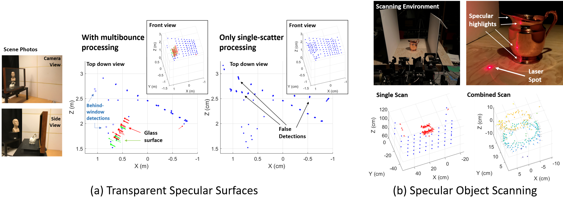
Figure 1: (a) We acquire the shape of a glass window (green and red points) and the scene surrounding it (blue points), which includes objects behind the window (white points, photos on left). When single-scatter paths are assumed (right), the window surface cannot be retrieved and numerous false points are generated. (b) We scan the shape of a copper pitcher (top) by directly illuminating a sequence of 60 laser spots on nearby surfaces and measuring the time-of-flight of two-bounce returns that reflect off of the pitcher (results bottom left). We repeat the scan four times, rotating the pitcher $90^{\circ}$ between scans, to acquire the full shape (bottom right).

The range to a surface is typically computed using the lidar range equation, which is only valid for single-scatter time-of-flight measurements. Thus, when the direct, single-scatter return from a specular surface is too faint to detect, it becomes impossible to compute the range to that surface via conventional means. Nevertheless, the presence of specular surfaces is often revealed by intense multibounce returns. For instance, when one directly illuminates a diffusely reflecting surface, nearby specular surfaces may produce mirror images of the true laser spot (also referred to as highlights) that appear just as bright as the original. Alternatively, when a specular surface is illuminated directly, the beam is often deflected such that it lands on a diffusely reflecting surface nearby.

In this work we demonstrate that multibounce returns are both an important cue that reveals the presence of specular surfaces, as well as an information source that can be used to estimate a specular reflector’s shape. We review the geometry of multibounce returns that are encountered in scenes that contain both diffuse and specular reflectors. Using our knowledge of this geometry, we propose criteria for unambiguously detecting the presence of specular multibounce signals, as well as a set of equations that relates the time- and angle-of-arrival of multibounce impulses to the position and orientation of points on the specular surface.

We apply our findings in a series of experiments in which we use multibounce lidar measurements to acquire the 3D shape of various specular objects. These objects include planar reflectors such as mirrors and windows, as well as a polished metal object with a freeform shape. For the special case of transparent surfaces, we propose criteria that can be used to distinguish between multibounce reflections off of the surface, and single-scatter returns from objects that lie behind the surface.

Our methods can be implemented using any lidar system for which the transmit and receive axes can be steered independently, or that uses a wide FOV receiver such as a single-photon avalanche diode (SPAD) array. For most of our experiments we use a pencil-beam illumination source that must be scanned to acquire a point cloud of the full scene. However we also propose an algorithm that can be used to map the surface of planar reflectors when the scene is illuminated by many beams simultaneously. Multi-beam illumination enables faster scene acquisition, and is employed by several commercial lidar scanners [1].

2 Related Work

2.0.1 Detecting Mirrors and Windows Using Lidar

Specular surfaces typically reflect most light away from the lidar receiver, resulting in very faint direct returns. When specular reflections are directed towards the receiver, the signal can be so intense that it saturates one’s detectors (this event is sometimes called “glare”). The presence of mirrors in a scene can also produce false detections of the mirror images of real objects, which typically appear behind the mirror.

To overcome these challenges, Diosi and Kleeman [4] use an ultrasonic scanner to detect specular surfaces that lidar scanners can’t see. Yang et al. [15] infer that framed gaps in detected surfaces likely contain mirrors or windows. After classifying mirrors in this way, they identify mirror image detections and reflect them across the mirror plane to the position of the true object. Foster et al. use sparse glare events to detect specular surfaces, but accumulate glare information over time in an occupancy grid as their laser scanner moves through a space [6]. Like Yang et al., Tibebu et al. [12] search for frames that are indicative of windows. However, to avoid detecting windowless holes, they use measurable pulse broadening caused by transmission through glass as a second heuristic to make their window detector more robust.

Unlike this previous work, our method does not rely on contextual cues like frame or mirror image detection that might be produced by non-specular scenes, we do not rely on rare glare events, and we do not require additional sensing modalities like ultrasound. The work that comes closest to ours was a speculative report by Raskar and Davis [9], who suggested that the time-of-flight of two-bounce returns could be used to localize specular surfaces, but did not demonstrate their method, and did not (as we do) consider the scenario where the specular surface is illuminated directly. Henley et al. [7] and Tsai et al. [13] estimate scene shape from two-bounce time-of-flight measurements, but neither consider the special conditions imposed by specular reflectors.

2.0.2 Specular Surface Estimation Using Cameras

There is an extensive body of literature that investigates methods for estimating the geometry of specular surfaces using conventional cameras that cannot capture time-of-flight information. A relatively recent review of this research was provided by Ihrke et al. [8]. A camera that observes a specular surface will see a distorted (if the mirror is curved) reflection of the scene that surrounds the surface. In most camera-based methods for specular geometry estimation, features in the distorted, reflected image are matched to features in the true scene. If the positions of the camera and true feature are known, then the depth and surface normal of the surface point that reflects the distorted feature can be determined up to a one-dimensional ambiguity. This ambiguity can be resolved in a variety of ways. In shape from specularity methods, the reflected scene features are point sources that produce specular highlights in the camera image [16][2]. In shape from distortion methods, a camera observes how specular reflection distorts the reflected image of a reference pattern [11][14][3]. In specular flow methods a camera observes how the distorted reflection of an uncalibrated scene appears to move across the surface of a specular object as the camera, object, or scene are moved [10].

Because we observe the specular reflection of laser spots, our method can be interpreted as a shape from specularity technique that uses time-of-flight constraints to resolve the depth-normal ambiguity. In future work, it would be interesting to explore the combination of time-of-flight constraints with other imaging strategies such as shape from distortion or specular flow.

3 Methods

3.1 Geometry of Specular Multibounce Signals

Consider the scenario illustrated in Fig. 2, where a mirror has been placed in an environment that is otherwise composed of diffusely reflecting surfaces. The mirror is a perfect specular reflector, which means that it will reflect all light from an incident beam in a single direction that is determined by the light’s direction of incidence and the mirror’s surface normal orientation. Our lidar system consists of a transmitter at position $L$ that emits a focused, pulsed beam in a single direction. A receiver array is placed at position $C$, which may be displaced from L by a baseline distance $\mathcal{s}$.

In this scenario the transmitter can illuminate either a diffuse reflector or the mirror directly. These two cases introduce distinct multibounce geometries that must be treated separately. In either case, our goal is to compute the position of all directly and indirectly illuminated points in the scene using the time-of-flight and angle-of-arrival of all observable direct and multibounce returns.

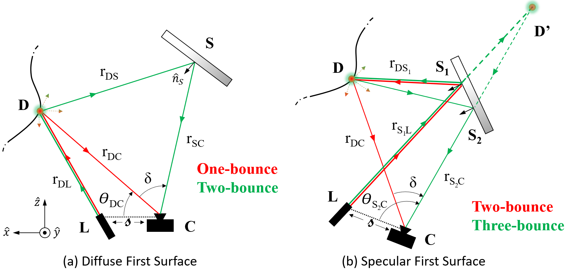
Figure 2: (a) A diffusely reflecting surface is illuminated directly at $D$. The camera observes one-bounce returns incident from $D$ and two-bounce returns incident from point $S$ on the mirror surface. (b) The specular surface is illuminated directly (at $S_{1}$) and the single-bounce return is too faint to observe. The camera observes two-bounce returns incident from $D$ and three-bounce returns incident from $S_{2}$.

3.1.1 First surface is a diffuse reflector.

In the first case, shown in Fig. 2(a), the transmitter directly illuminates a point $D$ on the diffusely reflecting surface. The receiver subsequently observes two laser spots: the true spot, which (correctly) appears to be located at $D$, and a mirror image of that spot. Light from the true spot has propagated along the single-bounce path $LDC$, whereas light that appears to originate from the spot’s mirror image has propagated along the two-bounce path $LDSC$. Here $S$ is the point at which light reflects off of the mirror. We use a method that was originally introduced in [7] to estimate the positions of $D$ and $S$ from the times- and angles-of-arrival of the one- and two-bounce returns. Angular positions are described by a clockwise rotation by $\theta$ about $\hat{y}$ followed by a clockwise rotation by $\phi$ about $\hat{x}$.

Light incident from the direction of the true spot $D$ will arrive at the angle ($\theta_{DC}$, $\phi_{DC}$) at time $t_{1}=\frac{1}{c}\left(r_{DL}+r_{DC}\right)$, where $r_{DL}$ and $r_{DC}$ are the distances to $D$ from $L$ and $C$, respectively. The distance to $r_{DC}$ can be computed using the following bi-static range equation:

$$r_{DC}=\frac{1}{2}\frac{c^{2}t_{1}^{2}-\mathcal{s}^{2}}{ct_{1}-\mathcal{s}cos(\theta_{DC})}.$$ (1)

Light incident from the direction of $S$ will arrive at the angle ($\theta_{SC}$, $\phi_{SC}$) at time $t_{2}=\frac{1}{c}\left(r_{DL}+r_{DS}+r_{SC}\right)$. Here $r_{DS}$ is the distance from $S$ to $D$ and $r_{SC}$ is the distance from $C$ to $S$. From simple arithmetic we see that $r_{DS}=c(t_{2}-t_{1})+r_{DC}-r_{SC}$. We plug this expression into the law of cosines for the triangle DCS to obtain

$$r_{SC}=\frac{c}{2}\cdot\frac{\Delta t_{12}[\Delta t_{12}+\frac{2r_{DC}}{c}]}{\Delta t_{12}+(1-\cos{\delta})\frac{r_{DC}}{c}}.$$ (2)

Here $\Delta t_{12}=t_{2}-t_{1}$ and $\delta$ is the apparent angular separation of the true spot and its mirror image, with $\cos{\delta}=\cos{\theta_{DC}}\cos{\theta_{SC}}+\sin{\theta_{DC}}\sin{\theta_{SC}}\cos{\left(\phi_{DC}-\phi_{SC}\right)}$.

We have now completely determined the positions of $S$ and $D$. We can additionally compute the surface normal at $S$ which, by the law of reflection, must be the normalized bisector of the angle formed by line segments $DS$ and $CS$.

3.1.2 First surface is a specular reflector.

In the second case, shown in Fig. 2(b), the mirror is illuminated directly at $S_{1}$. Because the mirror is a perfect specular reflector, no light that scatters at $S_{1}$ will travel directly back to the receiver, and so we do not observe a one-bounce return. Instead, all light in the beam is deflected such that it illuminates a spot $D$ on a diffusely reflecting surface. This laser spot is visible to the receiver. Once again, however, the receiver also sees a mirror image of the true laser spot. The mirror image of $D$ appears to lie behind the mirror at point $D^{\prime}$. This time, light that arrives from the true spot has traveled along the two-bounce path $LS_{1}DC$, and light that arrives from the spot’s mirror image follows the three-bounce path $LS_{1}DS_{2}C$.

Here we show that it is possible to compute the positions of $D$, $S_{1}$ and $S_{2}$ if $S_{1}$ and $S_{2}$ lie on the same plane. This condition is automatically satisfied if the specular surface is itself a plane, or if the baseline $\mathcal{s}=0$ (in which case $S_{1}=S_{2}$).

Our derivation hinges upon the observation that light that has actually followed the three-bounce trajectory $LS_{1}DS_{2}C$ will appear, from the perspective of the receiver, to have followed the one-bounce trajectory $LD^{\prime}C$, which includes a single scattering event at $D^{\prime}$. We can thus compute the apparent range to $D^{\prime}$ from the three-bounce travel time $t_{3}=\frac{1}{c}\left(r_{S_{1}L}+r_{DS_{1}}+r_{DS_{2}}+r_{S_{2}C}\right)=\frac{1}{c}\left(r_{D^{\prime}L}+r_{D^{\prime}C}\right)$. Using the range equation from Eq. 1, we obtain

$$r_{D^{\prime}C}=r_{DS_{2}}+r_{S_{2}C}=\frac{1}{2}\frac{c^{2}t_{3}^{2}-\mathcal{s}^{2}}{ct_{3}-\mathcal{s}cos(\theta_{S_{2}C})}.$$ (3)

The range to the illusory point $D^{\prime}$ is useful because it can be directly related to the range of the true point $D$ using the following expression:

$$r_{DC}=r_{D^{\prime}C}-c(t_{3}-t_{2}),$$ (4)

where $t_{2}=\frac{1}{c}\left(r_{S_{1}L}+r_{DS_{1}}+r_{DC}\right)$ is the two-bounce travel time. Once we’ve obtained $r_{DC}$ we compute the range to $S_{2}$ by substituting $r_{DS_{2}}=c(t_{3}-t_{2})+r_{DC}-r_{S_{2}C}$ into the law of cosines for the triangle $DCS_{2}$ to obtain

$$r_{S_{2}C}=\frac{c}{2}\cdot\frac{\Delta t_{23}[\Delta t_{23}+\frac{2r_{DC}}{c}]}{\Delta t_{23}+(1-\cos{\delta})\frac{r_{DC}}{c}},$$ (5)

where $\Delta t_{23}=t_{3}-t_{2}$ and $\delta$ once again refers to the apparent angular separation of the true spot and its mirror image. We note that if there are multiple specular surfaces in the scene then there may be multiple mirror image spots that are visible to the receiver. Only light from one of those mirror images can be used to compute $r_{DC}$ via Eq. 4. This will be the mirror image that appears to lie along the transmitted beam (in the direction of $S_{1}L$). However, the range to the reflection points on other specular surfaces can be computed once $r_{DC}$ is known. This is accomplished by plugging the angle-of-arrival and three-bounce time-of-flight associated with these other mirror image spots into Eq. 5.

If the direction of the transmitted beam is known then we can also compute the position of the directly illuminated point $S_{1}$. We begin by computing the apparent distance $r_{D^{\prime}L}$ from the laser to $D^{\prime}$:

$$r_{D^{\prime}L}=ct_{3}-r_{D^{\prime}C}=ct_{2}-r_{DC}.$$ (6)

The distance from $L$ to $S_{1}$ can then be computed using the identity $r_{DS_{1}}=r_{D^{\prime}L}-r_{S_{1}L}$ and the law of cosines from the triangle $S_{1}LD$. This distance is

$$r_{LS_{1}}=\frac{1}{2}\frac{r_{D^{\prime}L}^{2}-r_{DL}^{2}}{r_{D^{\prime}L}-r_{DL}\cos{\delta_{L}}},$$ (7)

where $r_{DL}=||D-L||_{2}$ and $\cos{\delta_{L}}=\frac{1}{r_{DL}}\left(D-L\right)\cdot\hat{d}_{S_{1}L}$. Here $\hat{d}_{S_{1}L}$ is the direction of the transmitted beam. Finally, from the law of reflection, we can compute the surface normal vectors at $S_{1}$ and $S_{2}$ once $D$, $S_{1}$ and $S_{2}$ are known.

3.1.3 Identifying the true spot and the first surface.

Although we have derived expressions that could in theory be used to compute the positions of all diffuse and specular scattering points within the scene, there are two ambiguities that need to be resolved before these expressions can be applied. First, we must determine whether the directly illuminated surface is a diffuse or a specular reflector. Doing so from raw measurements is not as straightforward as it might seem because in either case our receiver will see at least two spots, and one of these spots will appear to lie along the transmitter’s boresight. Second, regardless of which surface was illuminated first, we must also determine which observed spot is the true laser spot and which are mirror images.

Resolving the second ambiguity is always straightforward if we have time-of-flight information. Light from the true spot always arrives before the light from the mirror images. This can be confirmed by inspecting Fig. 2. In this figure all propagation paths travel through $D$. However, light from the true spot travels directly from $D$ to $C$, whereas light from the mirror images must follow a longer, indirect path that includes an additional reflection. The first-surface ambiguity can be resolved once the true spot has been identified. If the true spot lies along the transmitter boresight, then a diffuse reflector was illuminated first. If it doesn’t, then the specular surface was illuminated first. Once both ambiguities have been resolved, the appropriate range equations can be applied to determine the scattering points.

It is worth noting that we are only able to disambiguate these two cases because we have time-of-flight information. If we had instead been viewing the scene with a regular camera that only measured angles and intensities, then there would be no direct way to determine which spot was the true spot and which surface was illuminated first. Instead, we would have to rely on contextual cues to determine, for instance, which pixels seemed to have mirrors in them.

3.2 Transparent Specular Surfaces

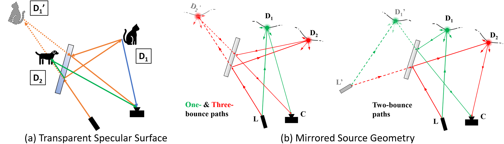
Figure 3: (a) When a transparent specular surface is illuminated directly, multiple laser spots may be detected along the beam vector—a true spot $D_{2}$ that lies behind the surface, and a mirror image ($D_{1}^{\prime}$) of a spot $D_{1}$ that lies in front of the surface. (b) Two-bounce paths (right) appear to originate at $L^{\prime}$, a mirror image of the true source. One- and three-bounce paths (left) appear to originate at the true source $L$.

Many of the most common specular surfaces—glass windows, for example—are partially transparent. Transparency introduces an additional source of ambiguity into our measurements, which is highlighted in Fig. 3(a). Here we see that, as was true for the mirror surface, three-bounce returns will typically resemble spots that lie behind the specular surface. When that surface is also transparent, however, these three-bounce returns may be mixed together with one-bounce returns that have scattered diffusely off of something that lies behind (or on) the specular surface. In this section we propose several criteria that can be used to detect and disambiguate these two kinds of signals.

Multiple Detections Along Beam.

Our disambiguation logic is triggered when we detect multiple spots lying along the transmitted beam vector. When this occurs, it suggests that we may have detected the mirror image of a true spot that lies in the scene in front of the window, in addition to a one-bounce return from a true spot that lies behind the window or on its surface.

Comparison to Two-bounce Travel Time.

When the window is illuminated directly, light that arrives from the true spot in front of the window follows a two-bounce path, and the spot will not lie on the beam vector. As was explained in Sec. 3.1, the mirror image in this scenario must correspond to a three-bounce return, and the associated three-bounce time-of-flight must be greater than the two-bounce time-of-flight from the true spot. Thus, if the time-of-flight associated with any of the spots that lie along the beam vector is less than the two-bounce time-of-flight, we deduce that they cannot be mirror image returns and, thus, must be single-scatter returns from on or behind the window surface.

Multiple Reflections Diminishes Intensity.

If the time-of-flight associated with more than one in-beam spot is greater than the two-bounce time-of-flight, we infer that the dimmest spot corresponds to the mirror image. The reasoning behind this is that three-bounce signals are reflected twice by the window, whereas one-bounce signals are transmitted twice. Common transparent, specular materials typically transmit more light than they reflect, although this assumption can break down at glancing incidence angles. To choose the dimmest spot, we rank in-beam detections by their range-adjusted intensity ($\sim r^{2}I$). For this computation, we use the apparent range of each spot, computed using Eq. 1.

3.3 Illumination with Multiple Beams

It is straightforward to employ the concepts introduced in Secs. 3.1 and 3.2 to acquire specular-surface geometry if the scene can be scanned by transmitting a single beam at a time. Unfortunately, the time required to do so may be unacceptably long for some applications. In this section we propose an algorithm that permits the mapping of specular surface geometry without any knowledge of spot-to-beam associations, and thus can be implemented when the scene is illuminated by a multi-beam flash.

3.3.1 Mirrored Source Geometry

If a transmitter emits a pulse at time $t$ in a scene that contains a flat mirror, then a receiver that is pointed at the mirror will observe a mirror image of the transmitter that also appears to emit a pulse at $t$. The direction that the mirrored pulse propagates will be flipped across the mirror plane. This geometry is visualized in Fig. 3(b), where the true source is at $L$, and its mirror image is at $L^{\prime}$. The position of $L^{\prime}$ is significant because the plane of the mirror perfectly bisects the line segment $LL^{\prime}$, and the plane’s surface normal is parallel to $LL^{\prime}$. This means that estimating the position of $L^{\prime}$ (relative to $L$) is equivalent to estimating the mirror plane. This is the key principle that underlies our multi-beam surface estimation algorithm.

The one-, two-, and three-bounce signals described in previous sections can also be interpreted under a mirrored space model. From the perspective of the receiver, one- and three-bounce returns appear to originate from the true source $L$. Two-bounce returns appear to originate from the mirrored source, at $L^{\prime}$. From Fig. 3(b), we see that the order of the bounces determines where the scattering event will appear to occur. If light bounces off of the mirror first, then the scattering event appears to occur in the true space at $D$. If it bounces off a diffuse reflector first, then light appears to scatter in the mirrored space at $D^{\prime}$.

3.3.2 Source Localization Using Multilateration

Because spots produced by one- or three-bounce light paths appear to originate from the true source, they must also lie along the axis of one of the true, transmitted beams. Spots that result from two-bounce light paths, on the other hand, will not in general lie along a transmitted beam vector. Because of this it is straightforward to determine which detected spots correspond to two-bounce light paths. An image of spot detections classified in a multi-beam data collection is shown in Fig. 6(b).

If we could compute the apparent positions of at least three two-bounce spots, then we could compute the ranges $r_{DL^{\prime}}=ct_{2}-r_{DC}$ or $r_{D^{\prime}L^{\prime}}=ct_{2}-r_{D^{\prime}C}$, and determine $L^{\prime}$ by solving a multilateration problem. Although we cannot compute these positions directly without knowledge of spot-to-beam associations, we can approximate them. From one-bounce returns, we compute the positions of several points in the true space using Eq. 1. We also compute the positions of a number of points in the mirrored space from three-bounce returns, using Eq. 3. We then approximate the positions of the two-bounce spots by interpolating from the positions of the nearest (in apparent angle) one- and three-bounce spots.

Once we’ve computed these approximate positions we can estimate the mirrored source position $L^{\prime}=[x_{0},y_{0},z_{0}]^{T}$ by solving the following optimization problem

$$\{x_{0},y_{0},z_{0}\}=\mathrm{arg}\min_{x_{0},y_{0},z_{0}}\frac{1}{2}\sum_{i}\left[(x_{i}-x_{0})^{2}+(y_{i}-y_{0})^{2}+(z_{i}-z_{0})^{2}-(ct_{i}-r_{i})^{2}\right]^{2}.$$ (8)

Here $(x_{i},y_{i},z_{i})$ is the approximate position (in $C$-centered coordinates) of the $i^{th}$ detected two-bounce spot, $r_{i}=\sqrt{x_{i}^{2}+y_{i}^{2}+z_{i}^{2}}$ and $t_{i}$ is the two-bounce travel-time associated with the $i^{th}$ spot. The objective function is twice-differentiable, so we can solve the problem using Newton’s method. In practice, misclassifications of two-bounce spots as one- or three-bounce spots, or vice-versa, produce large errors in the source localization result. To make our algorithm more robust to misclassification errors, we solve Eq. 8 using a RANSAC [5] approach that is robust to outliers.

3.3.3 Determining Scattering Points

As can be seen in Figure 3(b), rays drawn from the camera and from the true source to two-bounce points lying behind the mirror plane will intersect the mirror plane at reflection points, as will rays drawn from the mirrored source to two-bounce spots in front of the mirror plane. Thus, once the mirror plane has been computed from our estimate of $L^{\prime}$, we can find all points of specular reflection. From these reflection points we can also estimate the mirror’s boundary. This allows us to determine which spots correspond to three-bounce paths. The apparent positions of three-bounce spots can then be reflected across the mirror plane to retrieve the true diffuse scattering positions. This can be achieved even when the true scattering points lie outside of the receiver’s field-of-view (e.g. if they are hidden around a corner).

It is important to note that Eq. 8 only applies to planar specular surfaces, and so this algorithm will not produce accurate reconstructions of non-planar specular surfaces.

4 Results

4.1 Implementation

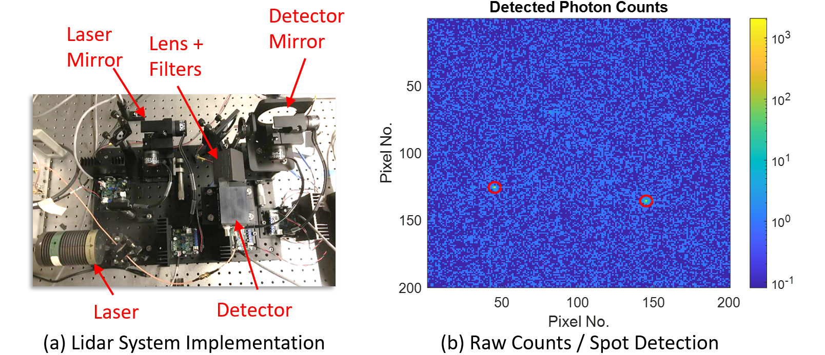
Figure 4: Implementation. (a) Our lidar system consists of a focused, pulsed galvo-scanned laser and a single-pixel SPAD that can be scanned independently of the laser. In our experiments the SPAD FOV is scanned across a dense, uniform grid to mimic the angular sampling pattern of a SPAD array camera. (b) Per-pixel map of detected photon counts. Detected spots are circled in red.

Lidar System.

A photo of our lidar system is provided in Fig. 4(a). The transmitter consists of a focused, pulsed laser source (640nm wavelength) that is scanned using a two-axis mirror galvanometer. The receiver is a single-pixel SPAD detector with a focused FOV that can be scanned independently from the laser using a second set of galvo mirrors. The overall instrument response function (IRF) of our system was measured to be 128 ps (FWHM). Details concerning the specific equipment used can be found in the supplemental material.

For each beam pointing direction, we reproduce the angular sampling pattern of a SPAD array camera by scanning the FOV of the detector across a dense, uniform grid. For experiments reported in this paper, the per-pixel dwell time was either 5 or 10 ms. The laser was operated at a pulse repetition frequency of 20 MHz and an average transmitted power of 5 $\mu W$.

Spot Extraction.

Raw photon count measurements are sorted into a data cube that is binned by photon time-of-arrival and detector scan angle. From these raw measurements we detect spot-like returns and then extract the time-of-flight, angle-of-arrival, and returned energy of each spot. An image of per-pixel detected photon counts collected from a single detector scan is shown in Fig. 4(b). Detected spots are circled in red. A more detailed description of our spot detection and low-level signal processing pipelines is provided in the Supplement.

4.2 Planar Surface Scans

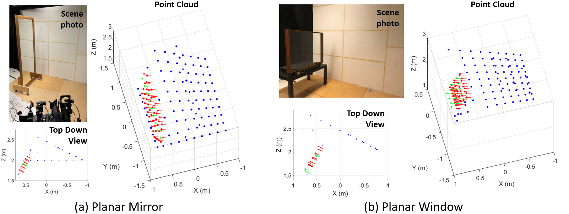
Figure 5: Scans of (a) a large flat mirror and (b) a single-pane glass window. Red and green points indicate points on specular surfaces, blue points indicate points on diffusely reflecting surfaces. Circles indicate diffuse-first illumination geometry and asterisks indicate specular-first geometry. Surface normals are also plotted at specular points.

4.2.1 Planar Mirror

We scanned a scene (shown in Figure 5(a)) that contained a tall, flat mirror, a wooden floor, and a matte white wall. The mirror was placed approximately 2m away from the lidar scanner. We scanned the laser beam along a $10\times 10$ grid of pointing directions. 14 beams illuminated the mirror directly. The remainder illuminated the floor, wall, or the mirror’s wooden frame. For each beam direction the detector FOV was scanned across a $200\times 200$ grid that subtended a $\pm 30^{\circ}$ angle of view in both vertical and horizontal directions. The per-pixel dwell time was 5 ms. Total acquisition time was 5 hours and 33 minutes, although we note that an equivalent data collection made using a $200\times 200$ pixel SPAD array would have been captured in 0.5 seconds.

Our results are shown in Fig. 5(a). Here, blue points represent points on diffuse surfaces, red points are points on the mirror as seen from the receiver ($S$ or $S_{2}$ in Fig. 2), and green points are points on the mirror that were illuminated directly ($S_{1}$ in Fig. 2). Points computed using diffuse-first equations are marked by circles, whereas points computed using specular-first equations are marked with asterisks. Surface normals are also plotted for specular surface points.

It is evident from Fig. 5(a) that the point cloud accurately captures the dimensions of the scene. From a comparison to a ground truth scan collected on the mirror’s frame, we determined that the points on the mirror surface had an RMS displacement of $9.5mm$ with respect to the ground truth plane, and the surface normals had an RMS tilt of $0.65^{\circ}$ with respect to the true surface normal. A complete evaluation of the scan’s accuracy is provided in the Supplement.

4.2.2 Planar Glass Window

We also scanned the shape of a single-pane glass window, which is shown in Fig. 5(b). The window was placed in the same position and orientation as the previously scanned mirror. For this collection we did not place any objects behind the window, and so the primary challenge was that the lower reflectance of the glass resulted in fainter multibounce returns, particularly for three-bounce light. We found that each reflection off the window reduced the range-adjusted intensity of a spot by approximately a factor of 10.

We compensated for the lower reflectance by doubling the per-pixel dwell time, to 10 ms. The laser scan pattern was changed to an $11\times 9$ grid that more densely sampled the portion of the scene that contained the window. The detector scan pattern was identical to that used in the mirror experiment. The total acquisition time was 11 hours, although we note that an equivalent data collection could have been captured by a SPAD array in just under one second.

Our results are shown in Fig. 5. The window pane can be seen clearly, and appears to have been mapped accurately. Despite the lower reflectance of the glass, we are able to detect all two-bounce and three-bounce returns with no misses or false alarms However, when the point cloud is viewed from the top-down it is clear that the points computed from three-bounce returns (marked by red and green asterisks) are noisier than two-bounce points. This was likely a consequence of the lower relative intensity of three-bounce returns.

4.2.3 Detecting Objects Behind a Window

We placed two objects behind the window and the repeated the window scan described previously. Our results are shown in Fig. 1(a). Behind-window detections are marked by white dots circled in blue. From these results we see that our disambiguation logic accurately classified four spots that scattered off of the objects behind the window. We note that all other points that appear to lie behind the window in the top-down view of the point cloud in fact lie above or below the window aperture.

In addition to the results shown here, we performed a second experiment that was designed to rigorously test the disambiguation criteria described in Section 3.2. These additional results can be found in the supplemental material in Section S.4.

Comparison to Naïve Single-bounce Processing.

On the right side of Fig. 1(a) we show the point cloud that would have been generated if the positions of all spots had been naïvely computed using the conventional one-bounce range equation. Notably, this naïve procesing detects no points on the window’s surface. Detections that might have been mapped to the window surface are instead mapped to erroneous points. Only true one-bounce returns are mapped correctly.

4.3 Non-planar Object Scans

Our method can also be used to acquire the shape of non-planar specular surfaces. We demonstrated this by scanning the shape of a copper pitcher. A photo of this pitcher and the results of our scan are shown in Fig. 1(b). The pitcher was placed on a wooden floor and in between two white side walls. We illuminated a sequence of 60 laser spots on these surfaces, and observed two-bounce returns that reflected off of the pitcher.

Laser spots and two-bounce highlights were acquired using a $200\times 100$ pixel scan with a 5 ms per-pixel dwell time. We repeated the scan four times, rotating the pitcher $90^{\circ}$ between each scan so that we could acquire it’s front, back, and side-facing surfaces. The four point clouds were aligned to a pitcher-centered coordinate system and then combined. From the combined point cloud in Fig. 1(b), we see that were are able to recover the general shape of the pitcher, although there are several gaps that correspond to regions that did not produce any detectable highlights due to their surface orientation.

We point out two distinctive features of the non-planar surface scanning process. First, because the pitcher’s surface alternated between convex, concave, and hyperbolic curvature, one laser spot would produce multiple highlights, each of which could be used to locate a point on the pitcher’s surface. This can be seen in the photograph on the top-right of Fig. 1. Second, Eqs. 4 and 5 are only correct when the tangent planes of surface points $S_{1}$ and $S_{2}$ are coincident. This is automatically satisfied for monostatic ($\mathcal{s}=0$) lidar systems, for which $S_{1}=S_{2}$. However, because our scanner was bi-static, these equations could not be applied for non-planar surface mapping. Consequently, all points in Fig. 1 had to be acquired by directly illuminating spots on diffuse reflectors, and observing two-bounce returns reflected by the pitcher. Specular-first returns could not be used. However, using the criteria outlined in Sec. 3.1, specular-first returns could be detected automatically and discarded.

4.4 Multiple-Beam Illumination

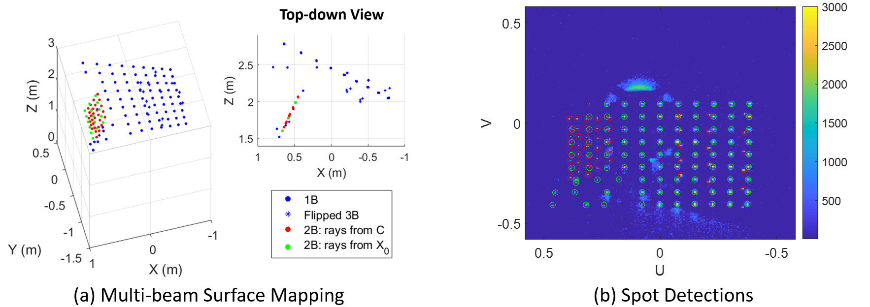
Figure 6: (a) Point-cloud generated using multi-beam surface mapping algorithm on glass window dataset (Fig. 5b). (b) Detected per-pixel energy values of multi-beam data collection, overlaid with spot positions. Red circles mark two-bounce spots, and green circles mark one- or three-bounce spots.

To test our multi-beam surface mapping algorithm, we summed the single-beam photon count histograms acquired during the first planar window scan described in Sec. 4.2. This produced the equivalent of a single multi-beam flash exposure. Detected per-pixel energy values from this multi-beam data are shown in Fig. 6(b). One- and three-bounce spots are circled in green, and two-bounce spots are circled in red.

Our results are shown in Fig. 6(a). By visual inspection we see that the window scattering points closely match the single-beam results in Fig. 5(b). Points in the multi-beam results in fact appear less noisy, although this is because they are intersections with a single, fitted plane. Many reflected three-bounce points appear in erroneous positions. Most of these points correspond to two-bounce spots that were incorrectly classified as three-bounce spots.

5 Discussion

We have demonstrated methods that use multibounce specular lidar returns to detect and map specular surfaces that might otherwise be invisible to lidar systems that rely on single-scatter measurements. We considered the cases of single-beam and multiple-beam illumination, and demonstrated our methods by scanning planar, non-planar, and transparent surfaces.

Because specular surfaces are relatively common, our work could be used in most domains that lidar scanning is applied to, including autonomous navigation, mapping of indoor or outdoor spaces, and object scanning. Future work might address failure cases, such as propagation paths with consecutive specular reflections, or geometries for which the true or mirror image spot lies outside the receiver FOV. We would also be interested in extending our multi-beam algorithm to the mapping of curved surfaces, and to allow dense flash illumination.

6 Acknowledgements

Connor Henley was supported by a Draper Scholarship. This material is based upon work supported by the Office of Naval Research under Contract No. N00014-21-C-1040. Any opinions, findings and conclusions or recommendations expressed in this material are those of the author(s) and do not necessarily reflect the views of the Office of Naval Research.

References

- [1] Apple, Inc.: Apple unveils new ipad pro with breakthrough lidar scanner and brings trackpad support to ipados. https://www.apple.com/newsroom/2020/03/apple-unveils-new-ipad-pro-with-lidar-scanner-and-trackpad-support-in-ipados/ (Mar 2020), accessed: 2021-10-28
- [2] Blake, A., Brelstaff, G.: Geometry from specularities. In: Proceedings of the 2nd International Conference on Computer Vision. pp. 394–403. IEEE (1988)
- [3] Bonfort, T., Sturm, P.: Voxel carving for specular surfaces. In: Proceedings of the Ninth International Conference on Computer Vision. IEEE (2003)
- [4] Diosi, A., Kleeman, L.: Advanced sonar and laser range finder fusion for simultaneous localization and mapping. In: 2004 IEEE/RSJ International Conference on Intelligent Robots and Systems (IROS) (IEEE Cat. No.04CH37566). vol. 2, pp. 1854–1859 (2004). https://doi.org/10.1109/IROS.2004.1389667
- [5] Fischler, M.A., Bolles, R.C.: Random sample consensus: A paradigm for model fitting with applications to image analysis and automated cartography. Commun. ACM 24(6), 381–395 (jun 1981). https://doi.org/10.1145/358669.358692
- [6] Foster, P., Sun, Z., Park, J.J., Kuipers, B.: Visagge: Visible angle grid for glass environments. In: 2013 IEEE International Conference on Robotics and Automation. pp. 2213–2220 (2013). https://doi.org/10.1109/ICRA.2013.6630875
- [7] Henley, C., Raskar, R.: Bounce-flash lidar. Optical Society of America (2021)
- [8] Ihrke, I., Kutulakos, K.N., Lensch, H.P.A., Magnor, M., Heidrich, W.: Transparent and specular object reconstruction. Computer Graphics Forum 29(8), 2400–2426 (2010), https://onlinelibrary.wiley.com/doi/abs/10.1111/j.1467-8659.2010.01753.x
- [9] Raskar, R., Davis, J.: 5 d time-light transport matrix : What can we reason about scene properties? (03 2008)
- [10] Roth, S., Black, M.: Specular flow and the recovery of surface structure. In: 2006 IEEE Computer Society Conference on Computer Vision and Pattern Recognition (CVPR’06). vol. 2, pp. 1869–1876 (2006). https://doi.org/10.1109/CVPR.2006.290
- [11] Savarese, S., Chen, M., Perona, P.: Local shape from mirror reflections. International Journal of Computer Vision 64(1), 31–67 (2005), https://doi.org/10.1007/s11263-005-1086-x
- [12] Tibebu, H., Roche, J., De Silva, V., Kondoz, A.: Lidar-based glass detection for improved occupancy grid mapping. Sensors 21(7) (2021), https://www.mdpi.com/1424-8220/21/7/2263
- [13] Tsai, C., Veeraraghavan, A., Sankaranarayanan, A.C.: Shape and reflectance from two-bounce light transients. In: 2016 IEEE International Conference on Computational Photography (ICCP). pp. 1–10 (2016). https://doi.org/10.1109/ICCPHOT.2016.7492882
- [14] Whelan, T., Goesele, M., Lovegrove, S., Straub, J., Green, S., Szeliski, R., Butterfield, S., Verma, S., Newcombe, R.: Reconstructing scenes with mirror and glass surfaces. ACM Transactions on Graphics 37(4) (aug 2018)
- [15] Yang, S.W., Wang, C.C.: On solving mirror reflection in lidar sensing. IEEE/ASME Transactions on Mechatronics 16(2), 255–265 (2011). https://doi.org/10.1109/TMECH.2010.2040113
- [16] Zisserman, A., Giblin, P., Blake, A.: The information available to a moving observer from specularities. Image Vision Comput. 7(1), 38–42 (1989), https://doi.org/10.1016/0262-8856(89)90018-8