On the Wasserstein median of probability measures

Abstract

Measures of central tendency such as mean and median are a primary way to summarize a given collection of random objects. In the field of optimal transport, the Wasserstein barycenter corresponds to Fréchet or geometric mean of a set of probability measures, which is defined as a minimizer of the sum of squared distances to each element in a given set when the order is 2. We present the Wasserstein median, an equivalent of Fréchet median under the 2-Wasserstein metric, as a robust alternative to the Wasserstein barycenter. We first establish existence and consistency of the Wasserstein median. We also propose a generic algorithm that makes use of any established routine for the Wasserstein barycenter in an iterative manner and prove its convergence. Our proposal is validated with simulated and real data examples when the objects of interest are univariate distributions, centered Gaussian distributions, and discrete measures on regular grids.

1 Introduction

The theory of optimal transport (OT) studies mathematical structure for the space of probability measures and is one of the most highlighted disciplines in modern data science. Originally introduced by Monge in the late 18th century (Monge, 1781), the OT problem was revisited with a generalized formulated of the problem by Kantrovich after almost two centuries since its inception (Kantorovitch, 1958). The framework of OT has long attracted much attention from theoretical perspectives (Ambrosio et al., 2003; Villani, 2003) and become more recognized by a wider audience since the advent of efficient computational pipelines (Cuturi, 2013; Peyré and Cuturi, 2019). This has engendered much success in quantitative fields. In machine learning, for example, the OT framework has been applied to numerous tasks such as metric learning (Kolouri et al., 2016), dimensionality reduction (Bigot and Klein, 2018), domain adaptation (Courty, Flamary, Tuia and Rakotomamonjy, 2017; Courty, Flamary, Habrard and Rakotomamonjy, 2017), and improving the generative adversarial networks (Arjovsky et al., 2017) to name a few.

Statistics has also benefited from developments in OT by incorporating core machineries into various problems (Panaretos and Zemel, 2020). A few notable examples include parameter estimation via minimum Wasserstein distance estimators (Bernton et al., 2019b), sampling from the posterior without Markov chain Monte Carlo methods (El Moselhy and Marzouk, 2012), two-sample hypothesis testing in high dimensions (Ramdas et al., 2017), approximate Bayesian computation (Bernton et al., 2019a), scalable Bayesian inference with a divide-and-conquer approach (Srivastava et al., 2018), and so on. Along these methodological innovations, a large volume of theoretical research has been simultaneously conducted to establish foundational knowledge in topics such as rate of convergence for Wasserstein distances (Fournier and Guillin, 2015) and optimal transport maps (Hütter and Rigollet, 2021), central limit theorems for the distance (del Barrio et al., 1999; Manole et al., 2021), and others.

At this moment, we call for attention to one of the most fundamental quantities in statistics to which a large number of aforementioned methods are related - the centroid. Suppose we are given a set of real numbers $x_{1},\ldots,x_{n}$ and their arithmetic mean $\bar{x}=\sum_{i=1}^{n}x_{i}/n$. The classical theory of statistics starts from examining how $\bar{x}$ behaves through the law of large numbers and the central limit theorem under certain conditions and proceeds to perform a number of inferential tasks thereafter. Not to mention distributional properties, $\bar{x}$ itself is often of importance to measure central tendency for a given set of observations since it represents maximally compressed information for a random sample. It is well known that $\bar{x}$ is heavily influenced by outliers and its robust alternative is the median, which is a minimizer of sum of absolute distances to the data. These centroids have been largely studied in the Euclidean space under the program of robust statistics (Huber, 1981) and generalized to other contexts. For instance, when data reside on a general metric space, these measures of central tendency correspond to the quantities called Fréchet mean and Fréchet median. For instance, their characteristics and properties have been well studied when the space of interest is some Riemannian manifolds (Kendall, 1990; Pennec, 2006; Afsari, 2011; Bhattacharya and Bhattacharya, 2012). In the field of OT, the concept of Fréchet mean is known as the Wasserstein barycenter, which minimizes sum of squared 2-Wasserstein distances. Since the seminal work of Agueh and Carlier (2011), its theoretical properties such as existence and uniqueness have been much studied along with computational studies that are of ongoing interests (Cuturi and Doucet, 2014; Dvurechenskii et al., 2018; Claici et al., 2018; Li et al., 2020; Xie et al., 2020; Korotin et al., 2021). Given the aforementioned reasoning with respect to measures of central tendency, one may naturally ask what corresponds to Fréchet median in the context of OT. Surprisingly, we have not been able to find an incumbent answer in the literature up to our knowledge.

This motivates our proposal of the Wasserstein median in response to the call. As its name entails, Wasserstein median generalizes Fréchet median onto the space of probability measures. A primary contribution of this paper is to formulate a novel measure of central tendency in the field of OT that fills a gap in the literature and prove its existence and consistency. Another appealing contribution is that we present an algorithm for computing a Wasserstein median whose convergence is also proved. Our proposed algorithm is generic in the sense that it can use any existing algorithms for computing Wasserstein barycenters. Although not rigorously investigated from a theoretical point of view, we speculate that the Wasserstein median has its potential as a robust alternative against the Wasserstein barycenter in the presence of outliers. Our numerical experiments provide ample evidence to support our conjecture.

The rest of this paper is organized as follows. In Section 2, we start our journey with a concise review on basic concepts in OT. We formulate the Wasserstein median problem and a generic algorithm in Section 3 along with relevant theoretical results. In Section 4, we discuss two special cases on how the Wasserstein median problem has its connection to the literature based on the arguments pertained to the computation. In Section 5, we validate the proposed framework with simulated and real data examples that come from popular modalities in OT. We conclude in Section 6 with discussion on issues and topics that help to pose potential directions for future studies. All proofs are deferred to Supplementary Materials.

2 Background

We start this section by introducing basic definitions and properties of the Wasserstein space and the metric structure defined thereon. Let $\mathcal{P}(\mathbb{R}^{d})$ the space of probability measures. The Wasserstein space of order $p$ on $\mathbb{R}^{d}$ is defined as

$$\mathcal{P}_{p}(\mathbb{R}^{d})=\left\{\mu\in\mathcal{P}(\mathbb{R}^{d}):\int_{\mathbb{R}^{d}}\|x\|^{p}\,d\mu(x)<\infty\right\},\quad p\geq 1,$$

where $\|\cdot\|$ is the standard norm in the Euclidean space. The distance for any $\mu,\nu\in\mathcal{P}_{p}(\mathbb{R}^{d})$ is defined as the minimum of total transportation cost by

$$\mathcal{W}_{p}(\mu,\nu)=\left(\underset{T:\mathbb{R}^{d}\rightarrow\mathbb{R}^{d}}{\inf}\int_{\mathbb{R}^{d}\times\mathbb{R}^{d}}\|x-T(x)\|^{p}\,d\mu(x)\right)^{1/p},$$ (1)

for a measurable transport map $T:\mathbb{R}^{d}\rightarrow\mathbb{R}^{d}$ such that $T_{\#}\mu=\nu$, i.e., for all measurable sets $B$, $\nu(B)=\mu(T^{-1}(B))$. The equation (1) is known as the Monge formulation (Monge, 1781). Although intuitive, the Monge formulation has some limitations that it does not allow split of masses and computation is prohibitive. A relaxed version of the formulation was proposed by Kantorovitch (1958) as follows. In the Kantrovich formulation, the distance between two measures $\mu,\nu\in\mathcal{P}_{p}(\mathbb{R}^{d})$ is defined as

$$\mathcal{W}_{p}(\mu,\nu)=\left(\underset{\pi\in\Pi(\mu,\nu)}{\inf}\int_{\mathbb{R}^{d}\times\mathbb{R}^{d}}\|x-y\|^{p}\,d\pi(x,y)\right)^{1/p},$$ (2)

where $\Pi(\mu,\nu)$ denotes a collection of all joint probability measures on $\mathbb{R}^{d}\times\mathbb{R}^{d}$ whose marginals are $\mu$ and $\nu$. Existence of an optimal joint measure from equation (2) is guaranteed under mild conditions (Villani, 2003).

It is well known that $\mathcal{W}_{p}$ is not only a metric on $\mathcal{P}_{p}(\mathbb{R}^{d})$ but also metrizes weak convergence of probabilities and the $p$-th moments (Villani, 2003). Besides the metric structure, the space of measures $\mathcal{P}_{p}(\mathbb{R}^{d})$ has other desirable properties such as completeness and separability (Villani, 2009). When the order is $p=2$, the 2-Wasserstein space $(\mathcal{P}_{2}(\mathbb{R}^{d}),\mathcal{W}_{2})$ can be viewed as a complete Riemannian manifold of non-negative curvature (Otto, 2001; Ambrosio et al., 2005). For an absolutely continuous measure $\mu\in\mathcal{P}_{2}(\mathbb{R}^{d})$ and an arbitrary $\nu\in\mathcal{P}_{2}(\mathbb{R}^{d})$, $T_{\mu}^{\nu}$ stands for an optimal transport map from $\mu$ to $\nu$ and $I:\mathbb{R}^{d}\rightarrow\mathbb{R}^{d}$ for an identity map. Then, a curve $\mu_{t}=[I+t(T_{\mu}^{\nu}-I)]\#\mu$ for $t\in[0,1]$ that interpolates the two measures as $\mu_{0}=\mu$ and $\mu_{1}=\nu$ is known as McCann’s interpolant (McCann, 1997), which is a constant-speed geodesic in $\mathcal{P}_{2}(\mathbb{R}^{d})$. This perspective naturally leads to define the tangent space of $\mathcal{P}_{2}(\mathbb{R}^{d})$ at $\mu$ by

$$\text{Tan}_{\mu}=\overline{\{t(T_{\mu}^{\nu}-I):~{}\nu\in\mathcal{P}_{2}(\mathbb{R}^{d}),~{}t>0\}}^{L_{2}(\mu)},$$

which is a subset of some Banach space $L_{2}(\mu)=\{f:\mathbb{R}^{d}\rightarrow\mathbb{R}^{d}~{}|~{}\int_{\mathbb{R}^{d}}\|f(x)\|^{2}d\mu(x)<\infty\}$. Using the map, one can define the exponential map $\exp_{\mu}:\text{Tan}_{\mu}\rightarrow\mathcal{P}_{2}(\mathbb{R}^{d})$ and the logarithmic map $\log_{\mu}:\mathcal{P}_{2}(\mathbb{R}^{d})\rightarrow\text{Tan}_{\mu}$, which is an inverse of the former, by

$$\exp_{\mu}(t(T_{\mu}^{\nu}-I))=[tT_{\mu}^{\nu}+(1-t)I]\#\mu\quad\textrm{ and }\quad\log_{\mu}(\nu)=T_{\mu}^{\nu}-I.$$

In the rest of this paper, we restrict our attention to the $p=2$ case. For notational simplicity, we may interchangeably write the barycenter and the median to denote the Wasserstein barycenter and the Wasserstein median of order 2 as long as they do not incur confusion in the context.

3 General problem

3.1 Problem statement

Let $\mu_{n}\in\mathcal{P}_{2}(\mathbb{R}^{d}),~{}n=1,\ldots,N$ be a collection of probability measures. The Wasserstein median $\nu^{*}$ is defined as a minimizer of the following functional

$$F(\nu)=\sum_{n=1}^{N}\pi_{n}\mathcal{W}_{2}(\nu,\mu_{n}),$$ (3)

for nonnegative weights $(\pi_{1},\ldots,\pi_{N})\in\Delta_{0}^{N}:=\{x\in\mathbb{R}^{N}~{}|~{}x_{i}>0,\,\sum_{i=1}^{N}x_{i}=1\}$. The minimization problem is well-defined since the Wasserstein distance $\mathcal{W}_{2}$ is non-negative and continuous. Given a sample version of the problem, it is natural to consider a population counterpart

$$F(\nu)=\mathbb{E}\mathcal{W}_{2}(\nu,\Lambda)=\int\mathcal{W}_{2}(\nu,\lambda)d\mathbb{P}(\lambda),$$ (4)

with respect to a random measure $\Lambda$ on $\mathcal{P}_{2}(\mathbb{R}^{d})$ with distribution $\mathbb{P}$. We note that the functional (3) can be viewed as an expectation with respect to a discrete measure $\Lambda=\sum_{n=1}\pi_{n}\delta_{\mu_{n}}$ on the space of probability measures.

We make a remark on the relationship between Wasserstein median and standard geometric median problems. Suppose we are given two dirac measures $\mu_{x}=\delta_{x}$ and $\mu_{y}=\delta_{y}$. By the definition (2), one can easily check that the Wasserstein distance of order 2 is reduced to the standard $L_{2}$ distance, i.e., $\mathcal{W}_{2}(\mu_{x},\mu_{y})=\|x-y\|$. Therefore, if we further restrict the class of desired centroids to be dirac measures, the Wasserstein median problem (3) translates to minimize the following objective function

$$F(\nu)=\sum_{n=1}^{N}\pi_{n}\|x-x_{n}\|,$$

for some $\nu=\delta_{x}$ and $\mu_{n}=\delta_{x_{n}}$. This is indeed equivalent to find a geometric median in the Euclidean setting so that we may consider the proposed Wasserstein median as a generalization to the space of probability measures.

3.2 Theoretical Results

Given the above formulation, we first study existence of a solution to the problem (4). Our strategy follows an argument of Bigot and Klein (2018) that show existence of a Wasserstein barycenter.

Proposition 3.1.

The functional $F(\nu)=\mathbb{E}\mathcal{W}_{2}(\nu,\Lambda)$ with respect to some random measure $\Lambda$ on $\mathcal{P}_{2}(\mathbb{R}^{d})$ admits a minimizer $\nu^{*}$.

Use of a random measure $\Lambda$ on $\mathcal{P}_{2}(\mathbb{R}^{d})$ with distribution $\mathbb{P}$ is supported by a fact that the space itself is a complete and separable metric space (Villani, 2003), which allows to define the “second degree” Wasserstein space $\mathcal{P}_{2}(\mathcal{P}_{2}(\mathbb{R}^{d}))$. This perspective motivated to investigate consistency of a Wasserstein barycenter (Le Gouic and Loubes, 2017). Consider a sequence of measures on $\mathcal{P}_{2}(\mathbb{R}^{d})$, all of which admit barycenters. If the sequence converges to some measure, a natural question is whether the sequence of corresponding barycenters also converges to that of a limiting measure, an answer of which turned out to be yes. For completeness, we present an equivalent statement for the Wasserstein median case.

Proposition 3.2 (Theorem 3 of Le Gouic and Loubes (2017)).

Let $\{\Lambda_{j}\}$ be a sequence of probability measures on $\mathcal{P}_{2}(\mathbb{R}^{d})$ that admits a corresponding set of Wasserstein medians $\{\nu_{j}\}$ for all $j\in\mathbb{N}$. Suppose $\mathcal{W}_{2}(\Lambda_{j},\Lambda)\rightarrow 0$ for some $\Lambda\in\mathcal{P}_{2}(\mathcal{P}_{2}(\mathbb{R}^{d}))$ as $j\rightarrow\infty$. Then the sequence $\{\nu_{j}\}$ has a limit point $\nu$, which is a Wasserstein median of $\Lambda$.

Consistency of a Wasserstein median derives immediate corollaries which we delineate in an informal manner. First, assume that $\Lambda$ has a unique median. For any sequence of measures $\{\Lambda_{j}\}$ that converges to $\Lambda$, its related sequence $\{\nu_{j}\}$ of Wasserstein medians converges to the unique median of $\Lambda$ (Le Gouic and Loubes, 2017). This further implies that any valid computational pipeline whose convergence is guaranteed can successfully estimate the optimal Wasserstein median if uniqueness conditions are ensured. Another direct implication is the law of large numbers for Wasserstein median. Consider $\Lambda_{j}$ as an empirical counterpart of $\Lambda$. Proposition 2.2.6 of Panaretos and Zemel (2020) claims that $\mathcal{P}_{2}(\Lambda_{n},\Lambda)\rightarrow 0$ if and only if $\Lambda\in\mathcal{P}_{2}(\mathcal{P}_{2}(\mathbb{R}^{d}))$. Application of Proposition 3.2 on top of almost sure convergence of $\Lambda_{j}\rightarrow\Lambda$ gives a rise to the law of large numbers in a weak sense. We close with a remark that these arguments require all Fréchet functionals to be finite.

3.3 Computation

We describe a geometric variant of the Weiszfeld algorithm (Weiszfeld, 1937; Fletcher et al., 2009) for the Wasserstein median problem by viewing the 2-Wasserstein space of probability measures $\mathcal{P}_{2}(\mathbb{R}^{d})$ as a Riemannian manifold (Ambrosio et al., 2021). In this section, a sequence of minimizers is denoted as $v^{(t)}$ at an iteration $t$.

We first describe direct application of the geometric Weiszfeld algorithm on $\mathcal{P}_{2}(\mathbb{R}^{d})$ using the transport-map based adaptation. First, the gradient of the cost function (3) can be written in terms of transport maps by

$$\nabla F(\nu)=-\sum_{n=1}^{N}\frac{\pi_{n}}{\mathcal{W}_{2}(\nu,\mu_{n})}\log_{v}(\mu_{n})=-\sum_{n=1}^{N}\frac{\pi_{n}}{\mathcal{W}_{2}(\nu,\mu_{n})}\left[T_{\nu}^{\mu_{n}}-I\right],$$

which resides on the tangent space of $\nu$. At every iteration, the geometric Weiszfeld algorithm updates a candidate by projecting the gradient back onto the Riemannian manifold $\mathcal{P}_{2}(\mathbb{R}^{d})$ via an exponential map

$$v^{(t+1)}=\exp_{v^{(t)}}\left(-\tau^{(t)}\nabla F(\nu^{(t)})\right),$$

with a varying step size $\tau^{(t)}=1/\sum_{n=1}^{N}w_{n}^{(t)}$ where $w_{n}^{(t)}=\pi_{n}/\mathcal{W}_{2}(\nu^{(t)},\mu_{n})$. Thus we may write the updating rule as

$$\nu^{(t+1)}=\exp_{v^{(t)}}\left(\frac{1}{\sum_{n=1}^{N}w_{n}^{(t)}}\nabla F(\nu^{(t)})\right)=\left[\sum_{n=1}^{N}\left(\tilde{w}_{n}^{(t)}T_{\nu^{(t)}}^{\mu_{n}}+(1-\tilde{w}_{n}^{(t)})I\right)\right]\#v^{(t)},$$ (5)

for a normalized weight vector $\tilde{w}_{n}^{(t)}=w_{n}^{(t)}/\sum_{n=1}^{N}w_{n}^{(t)}$. The geometric Weiszfeld algorithm follows a descent path by varying amounts of step size, which is determined by a fixed rule at each iteration. This mechanism helps to reduce the total computational complexity since a standard line search method requires repeated evaluations of the functional.

The transport map-based Weiszfeld algorithm, however, may not be a practical choice from a computational point of view. For example, the algorithm requires to compute $N$ transport maps $T_{v^{(t)}}^{\mu_{n}}$ at every iteration, which is an excessively prohibitive task in most cases. Instead, we take an alternative view of the Weiszfeld algorithm as an iteratively reweighted least squares (IRLS) method (Lawson, 1961; Rice, 1964; Osborne, 1985).

The IRLS algorithm is a type of gradient descent methods that solves an optimization problem involving a $p$-norm. A central idea behind the IRLS is to solve an abstruse problem by iteratively solving a sequence of weighted least square problems. Its simplicity has allowed widespread of the algorithm in a number of applications such as compressed sensing (Gorodnitsky and Rao, 1997; Chartrand and Wotao Yin, 2008; Daubechies et al., 2010) and parameter estimation in generalized linear models (Nelder and Wedderburn, 1972; McCullagh and Nelder, 1998).

In the Wasserstein median problem, we adapt the IRLS algorithm as follows. First, consider the following minimization functional at iteration $t$,

$$G_{t}(\nu)=\frac{1}{2}\sum_{n=1}^{N}\frac{\pi_{n}}{\mathcal{W}_{2}(\nu^{(t)},\mu_{n})}\mathcal{W}_{2}^{2}(\nu,\mu_{n})=\frac{1}{2}\sum_{n=1}^{N}{w_{n}^{(t)}}\mathcal{W}_{2}^{2}(\nu,\mu_{n}).$$ (6)

One can immediately observe that $G_{t}(\nu^{(t)})$ is half the minimum value attained at the $t$-th iteration. Using the similar machineries, the gradient of $G_{t}(\nu)$ is written as

$$\nabla G_{t}(\nu)=-\sum_{n=1}^{N}w_{n}^{(t)}\log_{v}(\mu_{n}).$$

One can directly check from the first-order condition that the updating rule (5) of the Weiszfeld algorithm is equal to solving the minimization problem (6) iteratively. Furthermore, scaling the weights $w_{n}^{(t)}$ by any positive scalar does not affect the solution of (6). Hence, we can rephrase the IRLS problem at iteration $t$,

$$\min_{\nu}G_{t}(\nu)=\min_{\nu}\sum_{n=1}^{N}\tilde{w}_{n}^{(t)}\mathcal{W}_{2}^{2}(\nu,\mu_{n}),$$ (7)

which corresponds to the standard formulation of the Wasserstein barycenter problem. This implies that the Wasserstein median problem is equivalent to solving a sequence of Wasserstein barycenter problems, the detailed procedure of which is described in Algorithm 1.

Algorithm 1 Wasserstein median computation by IRLS.

0:  a collection of probability measures $\{\mu_{n}\}_{n=1}^{N}$, weights $(\pi_{1},\ldots,\pi_{N})\in\Delta_{0}^{N}$.

0:  $\nu^{*}=\operatorname*{argmin}_{\nu\in\mathcal{P}_{2}(\mathbb{R}^{d})}\sum_{n=1}^{N}\pi_{n}\mathcal{W}_{2}(\nu,\mu_{n})$.

  Initialize $\nu^{(0)}$.

  repeat

     $w_{n}^{(t)}=\pi_{n}/\mathcal{W}_{2}(\nu^{(t)},\mu_{n})$.

     $\tilde{w}_{n}^{(t)}=w_{n}^{(t)}/\sum_{n=1}^{N}w_{n}^{(t)}$.

     $\nu^{(t+1)}=\operatorname*{argmin}_{\nu}G_{t}(\nu)=\operatorname*{argmin}_{\nu}\sum_{n=1}^{N}\tilde{w}_{n}^{(t)}\mathcal{W}_{2}^{2}(\nu,\mu_{n})$.

     if  $\nu^{(t+1)}$ is equal to one of $\mu_{n}$’s  then

        return $\nu^{(t+1)}$ and stop.

     end if

  until convergence.

Next, we show convergence of the prescribed procedure to a set of minima by arguing that the updating procedure induces a decreasing sequence in $\mathcal{P}_{2}(\mathbb{R}^{d})$. The following theorem establishes convergence of the proposed algorithm to a set of local minima.

Theorem 3.3.

Let $\{\mu_{n}\}_{n=1}^{N}\subset\mathcal{P}_{2}(\mathbb{R}^{d})$ be a collection of probability measures that are absolutely continuous with respect to the Lebesgue measure and corresponding weights $(\pi_{1},\ldots,\pi_{N})\in\Delta_{0}^{N}$. Define an updating function $U:\mathcal{P}_{2}(\mathbb{R}^{d})\rightarrow\mathcal{P}_{2}(\mathbb{R}^{d})$ such that $\nu^{(t+1)}=U(\nu^{(t)})=\operatorname*{argmin}_{\nu}G_{t}(\nu)$ as in (6). For an initial measure $\nu^{(0)}\in\mathcal{P}_{2}(\mathbb{R}^{d})$ such that $F(\nu^{(0)})<\infty$, the sequence $\{\nu^{(t)}\}$ for $t\in\mathbb{N}$ induced by the Algorithm 1 converges to a set $S=\{\nu\in\mathcal{P}_{2}(\mathbb{R}^{d})~{}|~{}F(U(\nu))=F(\nu)\}$.

We note that there are two stopping conditions in Algorithm 1. First, the iterative process terminates when an iterate $\nu^{(t+1)}$ corresponds to one of the inputs. This is because an adjusted weight in the following iteration diverges as a denominator becomes zero. An ad hoc remedy would be padding denominators of zeros with a very small number, which is equivalent to assigning an exceptionally large weight on the coinciding observation. In our experiments, we observed that such adjusting mechanism may not result in a meaningful update of an iterate in many cases. Second, a natural choice of stopping criterion would be a case when two consecutive iterates are close in terms of their Wasserstein distance, i.e., when $\mathcal{W}_{2}(\nu^{(t)},\nu^{(t+1)})<\epsilon$ for some small $\epsilon>0$. This is justified from a fact that $\mathcal{P}_{2}(\mathbb{R}^{d})$ is a complete metric space and convergence is upheld when a sequence is Cauchy. This stopping rule, however, may not be practical since computation of Wasserstein distance is a relatively expensive operation. An easy fix is to use alternative dissimilarity measures (You and Suh, 2022). In our experiments, we used the Frobenius distance between two consecutive covariance matrices for centered Gaussian measures example and the standard $L_{2}$ distance between marginal vectors in all other examples. We found no substantial differences between solutions when stopping criteria were set by these strategies and the Cauchy argument.

4 Special cases

4.1 One-dimensional distributions

The first special case is $d=1$. Let $\mu_{1}$ and $\mu_{2}$ are two probability measures on $\mathbb{R}$ with cumulative distribution functions $F_{1}$ and $F_{2}$. The 2-Wasserstein distance between two measures is defined as

$$\mathcal{W}_{2}(\mu_{1},\mu_{2})=\left(\int_{0}^{1}|F_{1}^{-1}(x)-F_{2}^{-1}(x)|^{2}dx\right)^{1/2}=\|F_{1}^{-1}-F_{2}^{-1}\|_{L_{2}(0,1)}=\|Q_{1}-Q_{2}\|_{L_{2}(0,1)},$$

where $Q_{i}$’s are quantile or inverse cumulative distribution functions, i.e., $Q_{i}(z)=\inf\{x\in\mathbb{R}~{}:~{}F_{i}(x)\geq z\}$. Given a collection of one-dimensional probability measures $\{\mu_{n}\}_{n=1}^{N}$ with quantile functions $\{Q_{n}\}_{n=1}^{N}$, the Wasserstein median problem is translated to finding a Fréchet median in the function space $L_{2}(0,1)$ as follows by omitting the subscript for notational simplicity throughout this section,

$$Q^{*}=\operatorname*{argmin}_{Q}\sum_{n=1}^{N}\pi_{n}\|Q-Q_{n}\|.$$

Since any absolutely continuous measure on $\mathbb{R}$ can be uniquely determined by its cumulative distribution function, the minimizer $Q^{*}$ can fully characterize the Wasserstein median $\nu^{*}$ of given probability measures.

In the IRLS formulation, updates are obtained by a sequence of minimization problems. At iteration $t$, the optimization problem is written as

$$\min_{Q}G_{t}(Q)=\min_{Q}\sum_{n=1}^{N}\tilde{w}_{n}^{(t)}\|Q-Q_{n}\|^{2},$$ (8)

where $w_{n}^{(t)}=\pi_{n}/\|Q^{(t)}-Q_{n}\|$ and $\tilde{w}_{n}^{(t)}=w_{n}^{(t)}/\sum_{n=1}^{N}w_{n}^{(t)}$. The solution of (8) is explicitly expressed as a weighted sum of $Q_{n}$’s,

$$Q^{(t+1)}=\operatorname*{argmin}_{Q}G_{t}(Q)=\sum_{n=1}^{N}\tilde{w}_{n}^{(t)}Q_{n},$$

which can be easily shown by solving for the Gateaux derivative of $G_{t}(Q)$. From a computational point of view, this accounts for updating the coefficients only without actually computing the quantity of interest at every iteration. We note that the Wasserstein median problem for one-dimensional probability measures admits a unique minimizer if quantile functions $Q_{1},\ldots,Q_{N}$ are not collinear (Vardi and Zhang, 2000; Minsker, 2015).

4.2 Gaussian measures

Another case of special interest is the space of non-degenerate Gaussian measures $\mathcal{N}_{2}(\mathbb{R}^{d})$, which is a strict subset of $\mathcal{P}_{2}(\mathbb{R}^{d})$. Given two multivariate Gaussian measures $\mu_{1}=N(m_{1},\Sigma_{1})$ and $\mu_{2}=N(m_{2},\Sigma_{2})$, the 2-Wasserstein distance is defined by

$$\mathcal{W}_{2}(\mu_{1},\mu_{2})=\left\{\|m_{1}-m_{2}\|^{2}+\text{Tr}\left(\Sigma_{1}+\Sigma_{2}-2(\Sigma_{1}\Sigma_{2})^{1/2}\right)\right\}^{1/2},$$

which has appeared in several studies (Dowson and Landau, 1982; Olkin and Pukelsheim, 1982; Givens and Shortt, 1984; Knott and Smith, 1984). McCann (1997) showed that the space of Gaussian measures is a totally geodesic submanifold of $\mathcal{P}_{2}(\mathbb{R}^{d})$. Based on the observation of $\mathcal{N}_{2}(\mathbb{R}^{d})$ as a submanifold, a Riemannian metric was proposed whose induced geodesic distance coincides with the 2-Wasserstein distance (Takatsu, 2011) and corresponding geometric operations were subsequently studied (Malagò et al., 2018). The Gaussian measure $N(m,\Sigma)$ is parametrized by two finite-dimensional parameters; a mean vector $m$ and a covariance matrix $\Sigma$. It is straightforward to see that $\mathcal{N}_{2}(\mathbb{R}^{d})$ is a product metric space of the Euclidean space $\mathbb{R}^{d}$ with trivial geometry and the space of centered Gaussian measures $\mathcal{N}_{0}^{d}$ endowed with a Riemannian metric. Hence, we limit our treatment of Gaussian distributions to $\mathcal{N}_{0}^{d}$ and interchangeably denote a centered Gaussian measure $N(0,\Sigma)$ as $N(\Sigma)$.

Let $\mu_{n}=N(\Sigma_{n})$ for $n=1,\ldots,N$ be a collection of non-degenerate centered Gaussian measures on $\mathbb{R}^{d}$. The Wasserstein median $\nu^{*}=N(\Sigma^{*})$ is a minimizer of the equivalent functional

$$F(\Sigma)=\sum_{n=1}^{N}\pi_{n}W_{2}(\Sigma,\Sigma_{n})=\sum_{n=1}^{N}\pi_{n}\left\{\text{Tr}\left(\Sigma+\Sigma_{n}-2(\Sigma\Sigma_{n})^{1/2}\right)\right\}^{1/2},$$ (9)

for a distance function $W_{2}$ restricted on $\mathcal{N}_{0}^{d}\times\mathcal{N}_{0}^{d}$,

$$W_{2}^{2}(\Sigma_{1},\Sigma_{2}):=\mathcal{W}_{2}^{2}(N(0,\Sigma_{1}),N(0,\Sigma_{2}))=\text{Tr}(\Sigma_{1}+\Sigma_{2}-2(\Sigma_{1}\Sigma_{2})^{1/2}).$$

At iteration $t$, a subproblem from the iterative IRLS formulation of minimizing (9) is written as

$$\min_{\Sigma}G_{t}(\Sigma)=\min_{\Sigma}\sum_{n=1}^{N}\tilde{w}_{n}^{(t)}W_{2}^{2}(\Sigma,\Sigma_{n}),$$ (10)

for $w_{n}^{(t)}=\pi_{n}/W_{2}(\Sigma^{(t)},\Sigma_{n})$ and $\tilde{w}_{n}^{(t)}=w_{n}^{(t)}/\sum_{n=1}^{N}w_{n}^{(t)}$. We notice that the subproblem (10) corresponds to computing the Wasserstein barycenter on $\mathcal{N}_{0}^{d}$. Here, we introduce two variants of fixed-point approaches to solve the problem. In order to minimize confusion induced by notation, we consider the following Wasserstein barycenter problem,

$$\underset{S\in\mathcal{N}_{0}^{d}}{\min}\,\sum_{n=1}^{N}\lambda_{n}W_{2}^{2}(S,\Sigma_{n}),$$

for $(\lambda_{1},\ldots,\lambda_{N})\in\Delta_{0}^{N}$ and use the subscript $S_{(k)}$ to denote iterations in the barycenter problem. Given an appropriate non-singular starting point $S_{(0)}\in\mathcal{N}_{0}^{d}$, the first algorithm by Rüschendorf and Uckelmann (2002) updates an iterate by

$$S_{(k+1)}=\sum_{n=1}^{N}\lambda_{n}\left(S_{(k)}^{1/2}\,\Sigma_{n}\,S_{(k)}^{1/2}\right)^{1/2},$$ (11)

where $S^{1/2}$ is square root of a symmetric, positive-definite matrix. Another iterative algorithm was proposed by Álvarez-Esteban et al. (2016) where a single-step update is performed by

$$S_{(k+1)}=S_{(k)}^{-1/2}\left(\sum_{n=1}^{N}\lambda_{n}\left(S_{(k)}^{1/2}\,\Sigma_{n}\,S_{(k)}^{1/2}\right)^{1/2}\right)^{2}S_{(k)}^{-1/2}.$$ (12)

While the latter update rule of (12) seems more complicated and incurs larger computational costs than (11), it was shown that a limit point of the iteration is a consistent estimator of the true barycenter (Álvarez-Esteban et al., 2016, Theorem 4.2). Computational routine for Wasserstein median of centered Gaussian measures under the IRLS formulation is summarized in Algorithm 2.

Algorithm 2 Wasserstein median of centered Gaussian measures.

0:  a collection of non-singular covariance matrices $\{\Sigma_{n}\}_{n=1}^{N}$, weights $(\pi_{1},\ldots,\pi_{N})\in\Delta_{0}^{N}$.

0:  $\Sigma^{*}=\operatorname*{argmin}_{\Sigma\in\mathcal{N}_{0}^{d}}\sum_{n=1}^{N}\pi_{n}W_{2}(\Sigma,\Sigma_{n})$.

  Initialize $\Sigma^{(0)}$.

  repeat

     $w_{n}^{(t)}=\pi_{n}/W_{2}(\Sigma^{(t)},\Sigma_{n})$.

     $\tilde{w}_{n}^{(t)}=w_{n}^{(t)}/\sum_{n=1}^{N}w_{n}^{(t)}$.

     Set $S_{(0)}=\Sigma^{(t)}$.

     repeat

        Update an iterate $S_{(k)}$ by

$$S_{(k+1)}=\begin{cases}\sum_{n=1}^{N}\tilde{w}_{n}^{(t)}\left(S_{(k)}^{1/2}\,\Sigma_{n}\,S_{(k)}^{1/2}\right)^{1/2},\,\,\textrm{ or }\\[10.0pt] S_{(k)}^{-1/2}\left(\sum_{n=1}^{N}\tilde{w}_{n}^{(t)}\left(S_{(k)}^{1/2}\,\Sigma_{n}\,S_{(k)}^{1/2}\right)^{1/2}\right)^{2}S_{(k)}^{-1/2}\end{cases}$$

     until convergence and denote the limit point as $S_{(*)}$.

     Update $\Sigma^{(t+1)}=S_{(*)}$.

     if  $\Sigma^{(t+1)}$ is equal to one of $\Sigma_{n}$’s  then

        return $\Sigma^{(t+1)}$ and stop.

     end if

  until convergence.

5 Examples

5.1 Univariate distributions

The first example is to compare how barycenter and median estimates behave differently where an object of interest is a set of univariate distributions. We consider the gamma distribution as a model probability measure to which our comparison is applied. In the rest of this experiment, we will denote the gamma distribution as Gamma($k,\theta$) where $k$ and $\theta$ are shape and scale parameters. We take two distributions Gamma(1,1) and Gamma(7.5, 0.75) as sources of signal (type 1) and contamination (type 2), respectively. As shown in Figure 1, the two distributions are highly disparate. To describe, Gamma(1,1) has a monotonically decreasing density function with concentrated mass near zero while Gamma(7.5, 0.75) has a mound-shape density.

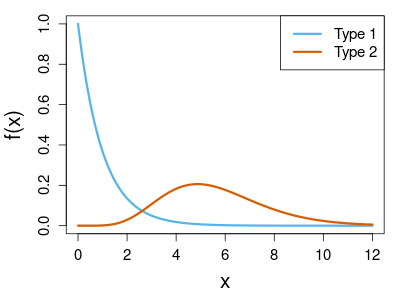
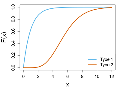
Figure 1: Two model Gamma distributions, Gamma(1,1) and Gamma(7.5, 0.75), are visualized via their (a) probability density functions (left) and (b) cumulative distribution functions (right).

Our experiment procedure is as follows. We generate perturbed versions of a distribution by drawing a random sample from the distribution and computing an empirical cumulative distribution function. This procedure is repeated $(100-k)$ times for Gamma(1,1) and $k$ times for Gamma(7.5, 0.75), leading to a collection of 100 empirical distributions. We set the number of sampling from type 2 measure as $k\in[1,25]$. Since we consider $k$ empirical distributions as contamination out of a total of 100 distributions, we will denote that the degree of contamination is $k\%$. When estimates of the two centroids are obtained, we quantify discrepancy between the estimates and the signal, i.e., Gamma(1,1), by the 2-Wasserstein distance.

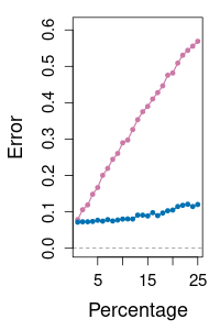
(a)

(b)

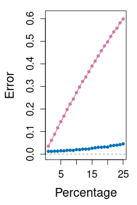
(c)

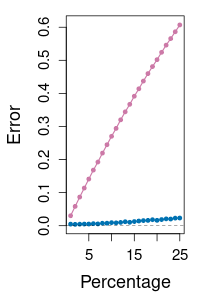
(d)

Figure 2: Performance comparison for the univariate distribution example. Average error of 50 runs is measured between the signal distribution and two centroid estimates, the Wasserstein barycenter (in purple) and the Wasserstein median (in blue), across varying degrees of contamination where the size of each random sample to reconstruct an empirical distribution is (a) 10, (b) 50, (c) 100, and (d) 500.

(a)

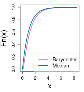
(b)

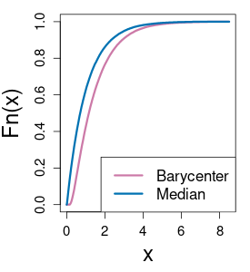
(c)

(d)

Figure 3: Visualization of the Wasserstein barycenter and median given a collection of 100 empirical distributions. Each empirical distribution is constructed from a corresponding random sample of size 500. The degrees of contamination are (a) $1\%$, (b) $5\%$, (c) $10\%$, and (d) $25\%$.

We summarize the results in Figure 2. Regardless of the sample size, one can observe a universal pattern that discrepancy between the barycenter and the signal distribution is magnified as the degree of contamination increases. In contrast, the added contamination does not seem to much affect the Wasserstein median. This pattern can be also verified as shown in Figure 3 where the estimated barycenter and median empirical distributions are visualized across different levels of contamination. When $k$ is small, two estimates are not much deviated from the cumulative distribution function of the signal as shown in Figure 1. However, as $k$ gets larger, the barycenter shows a large magnitude of deviation while the estimated median remains sufficiently close to the cumulative distribution function of the signal. This implies that the Wasserstein median is a robust measure of central tendency in the presence of contamination. This is indeed an expected behavior in the sense that the 2-Wasserstein geometry for cumulative distribution functions in $\mathbb{R}$ is equivalent to the Hilbertian structure of their quantile functions.

5.2 Centered Gaussian distributions

We apply the identical framework to the case where objects of interests are centered Gaussian distributions in $\mathbb{R}^{2}$. We take two Gaussian distributions $N(\Sigma_{1})$ and $N(\Sigma_{2})$ as sources of signal and contamination respectively where the covariances are given as

$$\Sigma_{1}=\begin{pmatrix}1&0\\ 0&1\end{pmatrix}\qquad\text{and}\qquad\Sigma_{2}=\begin{pmatrix}1&0.75\\ 0.75&1\end{pmatrix}.$$

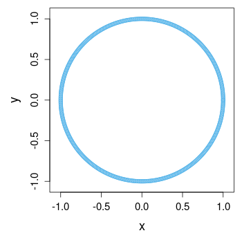
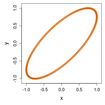
Figure 4: Two model covariance matrices $\Sigma_{1}$ (left in light blue) and $\Sigma_{2}$ (right in orange).

When two covariance matrices are graphically represented as shown in Figure 4, an identity matrix $\Sigma_{1}$ is drawn as a circle of radius 1 and $\Sigma_{2}$ is a rotated ellipse. Similar to the previous example, we generate perturbed variants of a distribution by computing a sample covariance for a randomly generated sample from the distribution. We repeat this process $(100-k)$ times for $N(\Sigma_{1})$ and $k$ times for $N(\Sigma_{2})$ for $k\in[1,25]$. This simulates a scenario where a majority of centered Gaussian measures resembles the signal measure $N(\Sigma_{1})$ and a small portion of perturbation comes from the contamination $N(\Sigma_{2})$. When barycenter and median estimates are obtained, we report discrepancy between the estimates and the signal measure $N(\Sigma_{1})$ by the Wasserstein distance of order 2.

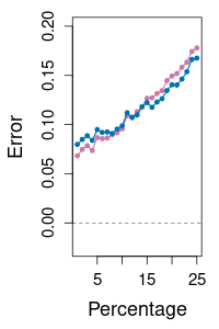
(a)

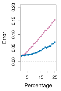
(b)

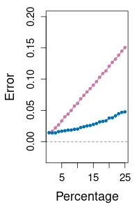
(c)

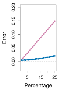
(d)

Figure 5: Performance comparison for the centered Gaussian distribution example. Average error of 50 runs is measured between the signal measure $N(\Sigma_{1})$ and two centroid estimates, the Wasserstein barycenter (in purple) and the Wasserstein median (in blue), across varying degrees of contamination where the size of a random sample for covariance estimation is (a) 10, (b) 50, (c) 100, and (d) 500.

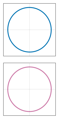
(a)

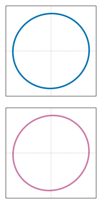
(b)

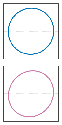
(c)

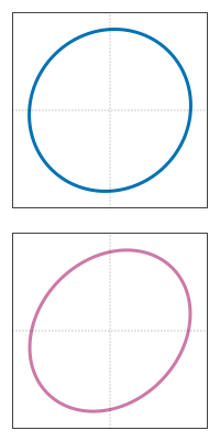
(d)

Figure 6: Visualization of the Wasserstein median (top row in blue) and the Wasserstein barycenter (bottom row in purple) given a collection of 100 centered Gaussian distributions consisting of two types. Each covariance matrix is estimated from a corresponding random sample of size 500. The degrees of contamination are (a) $1\%$, (b) $5\%$, (c) $10\%$, and (d) $25\%$.

The results are summarized in Figure 5. Except for the case where a random sample is of size 10, we see a consistent pattern as before that difference between the Wasserstein median and the signal measure remains almost consistent while that of the barycenter magnifies significantly as the degree of contamination increases. This is also validated in visual inspection of covariance estimates represented as ellipses in Figure 6 that the barycenter becomes more rotated with increasing eccentricity parallel to the degree of contamination. On the other stand, the median tends to be less deformed and remain close to the signal measure $N(\Sigma_{1})$, indicating its robustness in the presence of outliers.

5.3 Histograms and images

The last experiment applies the proposed framework to a set of discrete probability measures on regular grids, namely histograms and images. Both modalities have in common that the domain has lattice structure with finite support.

For the histogram example, we take the identical simulation setting. For a collection of histogram objects, a majority is drawn from signal measure and a small number of histograms are generated from contamination measure. In this example, we opt for the beta distribution denoted as Beta($\alpha,\beta$) for two shape parameters $\alpha>0$ and $\beta>0$ as a model distribution. We consider Beta(2,5) as the signal measure whose density function has a mound shape and positive skewness. For the contamination measure, we use Beta(5,1) whose density function is monotonically increasing in the bounded support. We use an equidistant partition $0=t_{0}<\cdots<t_{20}=1$ for binning a randomly generated sample and normalize bin counts as relative frequency so that the binned vector sums to 1.

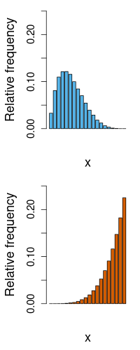
(a)

(b)

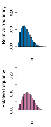
(c)

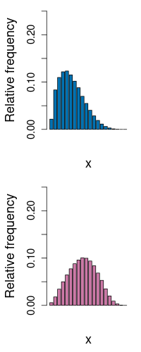
(d)

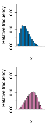
(e)

Figure 7: Visualization of the model beta distributions and the centroid estimates. The first column (a) presents density functions for the signal Beta(2,5) (top in light blue) and the contamination Beta(5,1) (bottom in orange). For the rest, estimated histograms of Wasserstein median (top row in blue) and the Wasserstein barycenter (bottom row in purple) are shown where each column corresponds to the varying degrees of contamination at (a) $1\%$, (b) $5\%$, (c) $10\%$, and (d) $25\%$. A random sample has the size of 250.

(a)

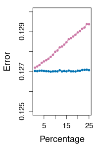
(b)

(c)

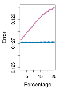
(d)

Figure 8: Performance comparison for the histogram example. Average error of 50 runs is measured between the signal measure Beta(2,5) and two centroid estimates, the Wasserstein median (in blue) and the Wasserstein barycenter (in purple), across varying degrees of contamination where a random sample is of size (a) 10, (b) 50, (c) 100, and (d) 500.

The designated model measures are shown in Figure 7 along with two centroid estimates across multiple levels of contamination. As the degree of contamination increases, estimated barycenters tend to deviate more from the signal measure while the medians remain nearly identical. This can be viewed in the sense of skewness where the barycenter becomes more negatively skewed for higher levels of contamination. Hence, we may argue that the barycenter altogether fails to characterize one of the basic properties for a desired measure of central tendency given a set of histograms. Our extended experiment to have 1 to 25 contaminants among a total of 100 histograms leads to the similar observation as presented in Figure 8 that the median outperforms the barycenter across all settings.

Lastly, we demonstrate how the Wasserstein median can benefit image analysis using the MNIST handwritten digits data (LeCun et al., 1998), which is one of the most popular image datasets in computer vision and image processing. In our experiment, we use normalized grayscale images for numeric digits 0 to 9 where all images are centered and rotated to rule out morphological variations. Each image is represented by a $28\times 28$ matrix where each entry takes a value in $[0,1]$. We also apply $L_{1}$ normalization so that elements in each image matrix sums to 1. This ensures to interpret an image as a valid probability measure on the 2-dimensional regular grid.

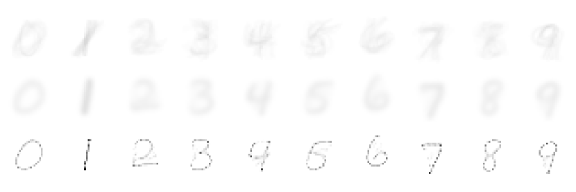
Figure 9: Visualization of the MNIST image example. Three rows represent the arithmetic mean (top), the Wasserstein barycenter (middle), and the Wasserstein median (bottom) of 50 images per digit.

We compare the arithmetic mean, the Wasserstein barycenter, and the Wasserstein median of 50 image matrices per digit, all of which are displayed in Figure 9. While the arithmetic means are largely blurred, the Wasserstein barycenters return readily recognizable images for each digit. Estimates of the Wasserstein median, however, reveal much more clandestine skeletal structure compared to the barycenters. This implies that the Wasserstein median is capable of sparsifying the support, engendering more compressed representation of images than the barycenter.

6 Conclusion

We proposed the Wasserstein median, a generalization of geometric median in Euclidean space onto the space of probability measures metrized by the Wasserstein distance of order 2. We provided theoretical results on existence and consistency of the Wasserstein median. A generic algorithm was proposed along with theoretical guarantee of its convergence. The proposed algorithm avoids repeated estimation of optimal transport maps, which itself is a computationally demanding task in most realistic circumstances. Furthermore, our computational pipeline is easily applicable to any settings where there exists a routine for the Wasserstein barycenter computation. We performed a set of experiments for various objects on which tools from OT has been elaborated, including univariate distributions, centered Gaussian distributions, and probability measures on regular grids. Across all experiments, we found strong empirical evidence to argue that the Wasserstein median is a robust alternative to the Wasserstein barycenter in the presence of contamination. We believe our proposed framework not only fills a rudimentary yet significant gap in the field of learning with probability measures under the optimal transport framework, but also lay foundation for its application to a variety of problems.

We close this paper by discussing a short list of topics for future studies. First, it is of utmost importance to examine on what conditions uniqueness of the Wasserstein median is guaranteed. On Riemannian manifolds, many have shown uniqueness of the geometric median using the convexity argument at the minima, which is not directly applicable since the Wasserstein space is not locally compact. Another essential element for the Wasserstein median is theoretical investigation of the robustness. In our study, we found abundant empirical evidence that the Wasserstein median is a robust measure of central tendency. This is somewhat expected as it generalizes the geometric median which is known to be robust in Euclidean space and Riemannian manifolds. Many of previous approaches in the literature, however, cannot be easily applied to the Wasserstein space as in the uniqueness argument. We believe theoretical contributions of such are essential in strengthening its potential as a valuable tool. Next, we believe that generalization of the base space is another promising direction. Our current exposition is on the Euclidean space where input measures are required to be absolutely continuous. In the literature on OT, trajectories in advancing the toolbox have attempted to generalize the fundamental theory into more general settings like locally compact geodesic space or arbitrary metric space. As modern statistics is frequently invited to work with heterogeneous types of data equipped with non-trivial structures, we often encounter situations by which critical assumptions in the casket of well-established theories cannot be abode. Lastly, we plan on building an improved computational framework for the Wasserstein median. Currently, our generic procedure makes iterative use of any algorithm that is designed to estimate Wasserstein barycenters. While convenient, this multiplies computational complexity by factor of the number of iterations. We suspect that one possible remedy is a stochastic algorithm that directly attempts to solve the problem. We believe development of efficient computational routines will make a compelling contribution to the field.

Supplementary Materials

Proof of Proposition 3.1

Proof.

If the functional $F(\nu)=\mathbb{E}\mathcal{W}_{2}(\nu,\Lambda)$ is identically infinite, the statement is valid for any choice of measure in $\mathcal{P}_{2}(\mathbb{R}^{d})$. If not, take a minimizing sequence $\{\nu_{j}\}\subset\mathcal{P}_{2}(\mathbb{R}^{d})$ and denote an upper bound of the functional with respect to the sequence as $C=\underset{j}{\sup}~{}F(\nu_{j})<\infty$. Assume $\nu_{0}$ be a fixed reference measure. By the triangle inequality, for a Dirac measure $\delta_{0}$ in $\mathcal{P}_{2}(\mathbb{R}^{d})$, we have

$$\mathbb{E}\mathcal{W}_{2}(\delta_{0},\Lambda) \leq \mathbb{E}\mathcal{W}_{2}(\delta_{0},\nu_{0})+\mathbb{E}\mathcal{W}_{2}(\nu_{0},\Lambda)$$

$$= \mathcal{W}_{2}(\delta_{0},\nu_{0})+\mathbb{E}\mathcal{W}_{2}(\nu_{0},\Lambda)$$

$$\leq \mathcal{W}_{2}(\delta_{0},\nu_{0})+C.$$

Therefore, the following holds for all $j$,

$$\mathbb{E}\mathcal{W}_{2}(\nu_{j},\delta_{0}) \leq \mathbb{E}\mathcal{W}_{2}(\nu_{j},\Lambda)+\mathbb{E}\mathcal{W}_{2}(\Lambda,\delta_{0})$$

$$\leq C+\mathcal{W}_{2}(\delta_{0},\nu_{0})+C$$

$$= 2C+\mathcal{W}_{2}(\delta_{0},\nu_{0})$$

$$= 2C+\left[\int_{\mathbb{R}^{d}}\|x\|^{2}d\nu_{0}(x)\right]^{1/2}<\infty,$$

and denote $\sup_{j}\mathbb{E}\mathcal{W}_{2}(\nu_{j},\delta_{0})=M<\infty$. For some $R>0$, the Chebyshev’s inequality states that

$$\nu_{j}\left(\left\{x\in\mathbb{R}^{d}~{}|~{}\|x\|\geq R\right\}\right)\leq\frac{1}{R^{2}}\int_{\{x:\|x\|\geq R\}}\|x\|^{2}d\nu_{n}(x)\leq\left(\frac{M}{R}\right)^{2}.$$

Take a sufficiently large $R$ such that $R>M^{2}/\sqrt{\epsilon}$ for a small $\epsilon>0$. Then, for a closed and bounded ball $B_{R}=\{x\in\mathbb{R}^{d}~{}|~{}\|x\|\leq R\}$, we have

$$\nu_{j}(B_{R})=1-\nu_{j}(B_{R}^{\mathsf{c}})>1-\epsilon\quad\text{for all }j,$$

which completes to show that sequence of measures $\{\nu_{j}\}$ is tight by the Heine-Borel theorem.

Since the sequence is tight, there exists a subsequence $\{\nu_{j_{k}}\}$ that converges weakly to some $\nu^{*}\in\mathcal{P}_{2}(\mathbb{R}^{d})$, which is characterized as a minimizer of the function since

$$F(\nu^{*})=\mathbb{E}\mathcal{W}_{2}(\nu^{*},\Lambda)\leq\mathbb{E}~{}\underset{j_{k}\rightarrow\infty}{\liminf}~{}\mathcal{W}_{2}(\nu_{j_{k}},\Lambda)\leq\underset{j_{k}\rightarrow\infty}{\liminf}~{}\mathbb{E}\mathcal{W}_{2}(\nu_{j_{k}},\Lambda)=\inf F,$$

where the first and second inequalities are by Fatou’s lemma and lower semicontinuity of the Wasserstein distance. This completes the proof. ∎

Proof of Proposition 3.2

Proof.

We rephrase the three-step strategy as in Le Gouic and Loubes (2017). The first step is to show that a sequence of Wasserstein medians $\{\nu_{j}\}$ is tight, which already appeared in the proof of Proposition 3.1. Therefore, we can take a subsequence $\{\nu_{j_{k}}\}\subset\{\nu_{j}\}$ that converges to some $\nu$.

Next, we show that the accumulation point $\nu$ is also a Wasserstein median. Take some $\xi\in\mathcal{P}_{2}(\mathbb{R}^{d})$ and a random measure $\mu\sim\Lambda$. Note that we employ a slightly different notation in what follows and this is for the purpose of distinguishing the first and the second degree Wasserstein spaces. Our goal is to show that $\mathbb{E}\mathcal{W}_{2}(\xi,\mu)\geq\mathbb{E}\mathcal{W}_{2}(\nu,\mu)$ for any choice of $\xi$ by similar arguments as before.

$$\mathbb{E}\mathcal{W}_{2}(\xi,\mu) =\mathcal{W}_{2}(\delta_{\xi},\Lambda)$$

$$=\lim_{j_{k}\rightarrow\infty}\mathcal{W}_{2}(\delta_{\xi},\Lambda_{j_{k}})$$

$$=\lim_{j_{k}\rightarrow\infty}\mathbb{E}\mathcal{W}_{2}(\xi,\mu_{j_{k}})\text{ for }\mu_{j_{k}}\sim\Lambda_{j_{k}}$$

$$\geq\lim_{j_{k}\rightarrow\infty}\mathbb{E}\mathcal{W}_{2}(\nu_{j_{k}},\mu_{j_{k}})$$ (13)

$$\geq\mathbb{E}\liminf_{j_{k}\rightarrow\infty}\mathcal{W}_{2}(\nu_{j_{k}},\mu_{j_{k}})\text{ by Fatou's lemma}$$

$$\geq\mathbb{E}\mathcal{W}_{2}(\nu,\mu).$$ (14)

The first inequality (13) holds because every element in $\{\nu_{j_{k}}\}$ is a Wasserstein median and the last inequality (14) is induced by the fact that Wasserstein distance is lower semicontinuous. Also, convergence of $\Lambda_{j_{k}}\rightarrow\Lambda$ enables to construct $\mu_{j_{k}}\rightarrow\mu$ almost surely by the Skorokhod’s representation theorem (Billingsley, 1999). Hence, we assert that any limit point $\nu$ of $\{\nu_{j}\}$ is indeed a Wasserstein median.

The last component is to show how $\nu$ is related to a limiting measure $\Lambda$. One implication of (14) is that we have $\mathcal{W}_{2}(\delta_{\nu_{j_{k}}},\Lambda_{j_{k}})\rightarrow\mathcal{W}_{2}(\delta_{\nu},\Lambda)$ if $\xi=\nu$. By the triangular inequality, we have

$$\mathcal{W}_{2}(\delta_{\nu_{j_{k}}},\Lambda)-\mathcal{W}_{2}(\delta_{\nu},\Lambda)\leq\mathcal{W}_{2}(\delta_{\nu_{j_{k}}},\Lambda_{j_{k}})+\mathcal{W}_{2}(\Lambda_{j_{k}},\Lambda)-\mathcal{W}_{2}(\delta_{\nu},\Lambda).$$

A repeated use of the previous tricks leads to

$$\liminf_{j_{k}\rightarrow\infty}\mathcal{W}_{2}(\nu_{j},\mu)=\mathcal{W}_{2}(\nu,\mu),$$

which implies $\mathcal{W}_{2}(\nu_{j_{k}},\xi)\rightarrow\mathcal{W}_{2}(\nu,\xi)$ for any $\xi\in\mathcal{P}_{2}(\mathbb{R}^{d})$ almost surely with respect to $\Lambda$. By the Theorem 2.2.1 of Panaretos and Zemel (2020), this is equivalent to $\mathcal{W}_{2}(\nu_{j_{k}},\nu)\rightarrow 0$, which completes the proof. ∎

Proof of Theorem 3.3

Proof.

We first show that the updating map $U:\mathcal{P}_{2}(\mathbb{R}^{d})\rightarrow\mathcal{P}_{2}(\mathbb{R}^{d})$ is a continuous function, which is defined by a suitable minimization problem in the IRLS formulation,

$$U(\tilde{\nu})=\operatorname*{argmin}_{\nu}\sum_{n=1}^{N}\frac{\pi_{n}}{\mathcal{W}_{2}(\tilde{\nu},\mu_{n})}\mathcal{W}_{2}^{2}(\nu,\mu_{n}).$$

Denote $\nu_{1},\nu_{2}$ be two arbitrarily close measures, i.e., $\mathcal{W}_{2}(\nu_{1},\nu_{2})<\delta$. By the triangle inequality, we have

$$\begin{gathered}\mathcal{W}_{2}(\nu_{1},\mu_{n})\leq\mathcal{W}_{2}(\nu_{1},\nu_{2})+\mathcal{W}_{2}(\nu_{2},\mu_{n})<\delta+\mathcal{W}_{2}(\nu_{2},\mu_{n}),\\ \mathcal{W}_{2}(\nu_{2},\mu_{n})\leq\mathcal{W}_{2}(\nu_{2},\nu_{1})+\mathcal{W}_{2}(\nu_{1},\mu_{n})<\delta+\mathcal{W}_{2}(\nu_{1},\mu_{n}),\end{gathered}$$

so that the inequality $|\mathcal{W}_{2}(\nu_{1},\mu_{n})-\mathcal{W}_{2}(\nu_{2},\mu_{n})|<\delta$ holds for all $n=1,\ldots,N$. Let $a_{n}=\mathcal{W}_{2}(\nu_{1},\mu_{n})$ and $b_{n}=\mathcal{W}_{2}(\nu_{2},\mu_{n})$. When we consider the following maps

$$U(\nu_{1})=\operatorname*{argmin}_{\nu}\sum_{n=1}^{N}\frac{\pi_{n}}{a_{n}}\mathcal{W}_{2}^{2}(\nu,\mu_{n}),\quad U(\nu_{2})=\operatorname*{argmin}_{\nu}\sum_{n=1}^{N}\frac{\pi_{n}}{b_{n}}\mathcal{W}_{2}^{2}(\nu,\mu_{n}),$$

the last inequality implies that one can control coefficients (or scaled weights) of the two updating maps to be sufficiently close by the following observation

$$\left|\frac{\pi_{n}}{a_{n}}-\frac{\pi_{n}}{b_{n}}\right|=\frac{\pi_{n}}{a_{n}b_{n}}\left|a_{n}-b_{n}\right|<\frac{\delta\pi_{n}}{a_{n}b_{n}}.$$

This further implies that the smaller the $\delta$ is, the closer two objective functions in the updating maps are. For any absolutely continuous measure $\mu$, the map $\nu\mapsto\mathcal{W}_{2}^{2}(\nu,\mu)$ is strictly convex and the solutions of two minimization problems uniquely exist (Bigot and Klein, 2018). Therefore, a sufficiently small $\delta$ can be set to bound the discrepancy between $U(\nu_{1})$ and $U(\nu_{2})$ by any $\epsilon>0$ as two continuous, strictly convex functionals converge as $\delta\rightarrow 0$.

Next, we show that the updating scheme induces a non-increasing sequence regarding the cost function $F$, which is equivalent to show that the inequality $F(U(\nu))\leq F(\nu)$ holds. At iteration $t$, the IRLS minimization problem is defined as

$$\min_{\nu}G_{t}(\nu)=\min_{\nu}\sum_{n=1}^{N}\frac{\pi}{\mathcal{W}_{2}(\nu^{(t)},\mu_{n})}\mathcal{W}_{2}^{2}(\nu,\mu_{n})=\min_{\nu}\sum_{n=1}^{N}\frac{\pi}{\mathcal{W}_{2}(\nu^{(t)},\mu_{n})}d^{2}(\log_{\nu^{(t)}}(\nu),\log_{\nu^{(t)}}(\mu_{n})),$$

where $d:\text{Tan}_{\nu^{(t)}}\times\text{Tan}_{\nu^{(t)}}\rightarrow\mathbb{R}$ is a distance function on the tangent space at $\nu^{(t)}$. An iterate $\nu^{(t+1)}$ is defined a minimizer of $G_{t}(\nu)$ so that $G_{t}(\nu^{(t+1)})\leq G_{t}(\nu^{(t)})$ and the equality holds if $\nu^{(t)}=\nu^{(t+1)}$ due to the uniqueness of barycenter. Since $\mathcal{P}_{2}(\mathbb{R}^{d})$ has nonnegative sectional curvature and is geodesically convex, we have $\mathcal{W}_{2}(\nu^{(t+1)},\mu_{n})\leq d(\log_{\nu^{(t)}}(\nu^{(t+1)}),\log_{\nu^{(t)}}(\mu_{n}))$ as a consequence of the Topogonov’s theorem. This leads to the following relationship,

$$F(\nu^{(t)}) = \sum_{n=1}^{N}\pi_{n}\mathcal{W}_{2}(\nu^{(t)},\mu_{n})$$

$$\geq \sum_{n=1}^{N}\frac{\pi_{n}}{\mathcal{W}_{2}(\nu^{(t)},\mu_{n})}\mathcal{W}_{2}^{2}(\nu^{(t+1)},\mu_{n})$$

$$= \sum_{N=1}^{N}\frac{\left(\pi_{n}\mathcal{W}_{2}(\nu^{(t+1)},\mu_{n})\right)^{2}}{\pi_{n}\mathcal{W}_{2}(\nu^{(t)},\mu_{n})},$$

which can be simplified as $\sum_{n=1}^{N}\alpha_{n}\geq\sum_{n=1}^{N}\beta_{n}^{2}/\alpha_{n}$ for $\alpha_{n}=\pi_{n}\mathcal{W}_{2}(\nu^{(t)},\mu_{n})$ and $\beta_{n}=\pi_{n}\mathcal{W}_{2}(\nu^{(t+1)},\mu_{n})$. If we define a univariate function $h(x)=\sum_{n=1}^{N}\alpha_{n}^{1-x}\beta_{n}^{x}=\sum_{n=1}^{N}\alpha_{n}(\beta_{n}/\alpha_{n})^{x}$, the above relationship is paraphrased as $h(0)\geq h(2)$. Since $h$ is a convex function as $d^{2}h/dx^{2}\geq 0$, the following holds

$$h(1)=h\left(\frac{1}{2}\cdot 0+\frac{1}{2}\cdot 2\right)\leq\frac{1}{2}h(0)+\frac{1}{2}h(2)\leq h(0),$$

which proves our claim since

$$\sum_{n=1}^{N}\pi_{n}\mathcal{W}_{2}(\nu^{(t+1)},\mu_{n})=h(1)\leq h(0)=\sum_{n=1}^{N}\pi_{n}\mathcal{W}_{2}(\nu^{(t)},\mu_{n}),$$

and equality holds if $\mathcal{W}_{2}(\nu^{(t)},\mu_{n})=\mathcal{W}_{2}(\nu^{(t+1)},\mu_{n})$ for all $n$.

Now we prove the main part of the theorem. Let $\{\nu^{(t)}\}$ be a sequence of updates starting from $\nu^{(0)}$. Since $F(\nu^{(0)})<\infty$ and the IRLS updating rule engenders a non-increasing sequence, we can take a minimizing sequence $\{\nu^{(t_{k})}\}_{k=1}^{\infty}$ that converges to some $\nu^{*}$ in the sense that $\lim_{k\rightarrow\infty}\,F(\nu^{(t_{k})})=F(\nu^{*})$, which leads to the following observation that

$$\lim_{k\rightarrow\infty}\,F(U(\nu^{(t_{k})}))=F(U(\nu^{*})),$$

by the continuity of an updating map. Moreover, $\{F(\nu^{(t)})\}_{t=1}^{\infty}$ is a bounded and non-increasing sequence in $\mathbb{R}$ so that there exists an accumulation point and it must correspond to that of a convergent subsequence. Therefore, we end up with

$$F(U(\nu^{*}))=\lim_{k\rightarrow\infty}F(U(\nu^{(t_{k})}))=\lim_{k\rightarrow\infty}F(\nu^{(t_{k})})=\lim_{t\rightarrow\infty}F(\nu^{(t)})=F(\nu^{*}),$$

where an accumulation point $\nu^{*}$ of the sequence belongs to a set of stationary points $S$ as stated in the theorem. ∎

References

- (1)
- Afsari (2011) Afsari, B. (2011). Riemannian $L{̂p}$ center of mass: Existence, uniqueness, and convexity, Proceedings of the American Mathematical Society 139(02): 655–655.
- Agueh and Carlier (2011) Agueh, M. and Carlier, G. (2011). Barycenters in the Wasserstein Space, SIAM Journal on Mathematical Analysis 43(2): 904–924.
- Álvarez-Esteban et al. (2016) Álvarez-Esteban, P. C., del Barrio, E., Cuesta-Albertos, J. and Matrán, C. (2016). A fixed-point approach to barycenters in Wasserstein space, Journal of Mathematical Analysis and Applications 441(2): 744–762.
- Ambrosio et al. (2021) Ambrosio, L., Brué, E. and Semola, D. (2021). Lectures on Optimal Transport, number volume 130 in Unitext - La Matematica per Il 3 + 2, Springer, Cham.
- Ambrosio et al. (2003) Ambrosio, L., Caffarelli, L. A. and Salsa, S. (eds) (2003). Optimal Transportation and Applications: Lectures given at the C.I.M.E. Summer School Held in Martina Franca, Italy, September 2-8, 2001, number 1813 in Lecture Notes in Mathematics, Springer, Berlin ; New York.
- Ambrosio et al. (2005) Ambrosio, L., Gigli, N. and Savaré, G. (2005). Gradient Flows: In Metric Spaces and in the Space of Probability Measures, Lectures in Mathematics ETH Zürich, Birkhäuser, Boston.
- Arjovsky et al. (2017) Arjovsky, M., Chintala, S. and Bottou, L. (2017). Wasserstein generative adversarial networks, in D. Precup and Y. W. Teh (eds), Proceedings of the 34th International Conference on Machine Learning, Vol. 70 of Proceedings of Machine Learning Research, PMLR, pp. 214–223.
- Bernton et al. (2019a) Bernton, E., Jacob, P. E., Gerber, M. and Robert, C. P. (2019a). Approximate Bayesian computation with the Wasserstein distance, Journal of the Royal Statistical Society: Series B (Statistical Methodology) 81(2): 235–269.
- Bernton et al. (2019b) Bernton, E., Jacob, P. E., Gerber, M. and Robert, C. P. (2019b). On parameter estimation with the Wasserstein distance, Information and Inference: A Journal of the IMA 8(4): 657–676.
- Bhattacharya and Bhattacharya (2012) Bhattacharya, A. and Bhattacharya, R. (2012). Nonparametric Inference on Manifolds: With Applications to Shape Spaces, Cambridge University Press, Cambridge.
- Bigot and Klein (2018) Bigot, J. and Klein, T. (2018). Characterization of barycenters in the Wasserstein space by averaging optimal transport maps, ESAIM: Probability and Statistics 22: 35–57.
- Billingsley (1999) Billingsley, P. (1999). Convergence of Probability Measures, Wiley Series in Probability and Statistics. Probability and Statistics Section, 2nd ed edn, Wiley, New York.
- Chartrand and Wotao Yin (2008) Chartrand, R. and Wotao Yin (2008). Iteratively reweighted algorithms for compressive sensing, 2008 IEEE International Conference on Acoustics, Speech and Signal Processing, IEEE, Las Vegas, NV, USA, pp. 3869–3872.
- Claici et al. (2018) Claici, S., Chien, E. and Solomon, J. (2018). Stochastic Wasserstein barycenters, in J. Dy and A. Krause (eds), Proceedings of the 35th International Conference on Machine Learning, Vol. 80 of Proceedings of Machine Learning Research, PMLR, pp. 999–1008.
- Courty, Flamary, Habrard and Rakotomamonjy (2017) Courty, N., Flamary, R., Habrard, A. and Rakotomamonjy, A. (2017). Joint distribution optimal transportation for domain adaptation, in I. Guyon, U. V. Luxburg, S. Bengio, H. Wallach, R. Fergus, S. Vishwanathan and R. Garnett (eds), Advances in Neural Information Processing Systems, Vol. 30, Curran Associates, Inc.
- Courty, Flamary, Tuia and Rakotomamonjy (2017) Courty, N., Flamary, R., Tuia, D. and Rakotomamonjy, A. (2017). Optimal Transport for Domain Adaptation, IEEE Transactions on Pattern Analysis and Machine Intelligence 39(9): 1853–1865.
- Cuturi (2013) Cuturi, M. (2013). Sinkhorn distances: Lightspeed computation of optimal transport, in C. Burges, L. Bottou, M. Welling, Z. Ghahramani and K. Weinberger (eds), Advances in Neural Information Processing Systems, Vol. 26, Curran Associates, Inc.
- Cuturi and Doucet (2014) Cuturi, M. and Doucet, A. (2014). Fast computation of wasserstein barycenters, in E. P. Xing and T. Jebara (eds), Proceedings of the 31st International Conference on Machine Learning, Vol. 32 of Proceedings of Machine Learning Research, PMLR, Bejing, China, pp. 685–693.
- Daubechies et al. (2010) Daubechies, I., DeVore, R., Fornasier, M. and Güntürk, C. S. (2010). Iteratively reweighted least squares minimization for sparse recovery, Communications on Pure and Applied Mathematics 63(1): 1–38.
- del Barrio et al. (1999) del Barrio, E., Giné, E. and Matrán, C. (1999). Central Limit Theorems for the Wasserstein Distance Between the Empirical and the True Distributions, The Annals of Probability 27(2).
- Dowson and Landau (1982) Dowson, D. and Landau, B. (1982). The Fréchet distance between multivariate normal distributions, Journal of Multivariate Analysis 12(3): 450–455.
- Dvurechenskii et al. (2018) Dvurechenskii, P., Dvinskikh, D., Gasnikov, A., Uribe, C. and Nedich, A. (2018). Decentralize and randomize: Faster algorithm for wasserstein barycenters, in S. Bengio, H. Wallach, H. Larochelle, K. Grauman, N. Cesa-Bianchi and R. Garnett (eds), Advances in Neural Information Processing Systems, Vol. 31, Curran Associates, Inc.
- El Moselhy and Marzouk (2012) El Moselhy, T. A. and Marzouk, Y. M. (2012). Bayesian inference with optimal maps, Journal of Computational Physics 231(23): 7815–7850.
- Fletcher et al. (2009) Fletcher, P. T., Venkatasubramanian, S. and Joshi, S. (2009). The geometric median on Riemannian manifolds with application to robust atlas estimation, NeuroImage 45(1): S143–S152.
- Fournier and Guillin (2015) Fournier, N. and Guillin, A. (2015). On the rate of convergence in Wasserstein distance of the empirical measure, Probability Theory and Related Fields 162(3-4): 707–738.
- Givens and Shortt (1984) Givens, C. R. and Shortt, R. M. (1984). A class of Wasserstein metrics for probability distributions., Michigan Mathematical Journal 31(2).
- Gorodnitsky and Rao (1997) Gorodnitsky, I. and Rao, B. (1997). Sparse signal reconstruction from limited data using FOCUSS: A re-weighted minimum norm algorithm, IEEE Transactions on Signal Processing 45(3): 600–616.
- Huber (1981) Huber, P. J. (1981). Robust Statistics, Wiley Series in Probability and Mathematical Statistics, Wiley, New York.
- Hütter and Rigollet (2021) Hütter, J.-C. and Rigollet, P. (2021). Minimax estimation of smooth optimal transport maps, The Annals of Statistics 49(2).
- Kantorovitch (1958) Kantorovitch, L. (1958). On the Translocation of Masses, Management Science 5(1): 1–4.
- Kendall (1990) Kendall, W. S. (1990). Probability, Convexity, and Harmonic Maps with Small Image I: Uniqueness and Fine Existence, Proceedings of the London Mathematical Society s3-61(2): 371–406.
- Knott and Smith (1984) Knott, M. and Smith, C. S. (1984). On the optimal mapping of distributions, Journal of Optimization Theory and Applications 43(1): 39–49.
- Kolouri et al. (2016) Kolouri, S., Zou, Y. and Rohde, G. K. (2016). Sliced wasserstein kernels for probability distributions, Proceedings of the IEEE Conference on Computer Vision and Pattern Recognition (CVPR).
- Korotin et al. (2021) Korotin, A., Li, L., Solomon, J. and Burnaev, E. (2021). Continuous wasserstein-2 barycenter estimation without minimax optimization, International Conference on Learning Representations.
- Lawson (1961) Lawson, C. L. (1961). Contributions to the Theory of Linear Least Maximum Approximation, PhD thesis, University of California Los Angeles.
- Le Gouic and Loubes (2017) Le Gouic, T. and Loubes, J.-M. (2017). Existence and consistency of Wasserstein barycenters, Probability Theory and Related Fields 168(3-4): 901–917.
- LeCun et al. (1998) LeCun, Y., Cortes, C. and Burges, C. (1998). The MNIST Database of Handwritten Digits, http://yann.lecun.com/exdb/mnist/.
- Li et al. (2020) Li, L., Genevay, A., Yurochkin, M. and Solomon, J. M. (2020). Continuous regularized wasserstein barycenters, in H. Larochelle, M. Ranzato, R. Hadsell, M. Balcan and H. Lin (eds), Advances in Neural Information Processing Systems, Vol. 33, Curran Associates, Inc., pp. 17755–17765.
- Malagò et al. (2018) Malagò, L., Montrucchio, L. and Pistone, G. (2018). Wasserstein Riemannian geometry of Gaussian densities, Information Geometry 1(2): 137–179.
- Manole et al. (2021) Manole, T., Balakrishnan, S., Niles-Weed, J. and Wasserman, L. (2021). Plugin Estimation of Smooth Optimal Transport Maps.
- McCann (1997) McCann, R. J. (1997). A Convexity Principle for Interacting Gases, Advances in Mathematics 128(1): 153–179.
- McCullagh and Nelder (1998) McCullagh, P. and Nelder, J. A. (1998). Generalized Linear Models, number 37 in Monographs on Statistics and Applied Probability, 2nd ed edn, Chapman & Hall/CRC, Boca Raton.
- Minsker (2015) Minsker, S. (2015). Geometric median and robust estimation in Banach spaces, Bernoulli 21(4).
- Monge (1781) Monge, G. (1781). Mémoire Sur La Théorie Des Déblais et Des Remblais, De l’Imprimerie Royale.
- Nelder and Wedderburn (1972) Nelder, J. A. and Wedderburn, R. W. M. (1972). Generalized Linear Models, Journal of the Royal Statistical Society. Series A (General) 135(3): 370.
- Olkin and Pukelsheim (1982) Olkin, I. and Pukelsheim, F. (1982). The distance between two random vectors with given dispersion matrices, Linear Algebra and its Applications 48: 257–263.
- Osborne (1985) Osborne, M. R. (1985). Finite Algorithms in Optimization and Data Analysis, Wiley Series in Probability and Mathematical Statistics, Wiley, Chichester ; New York.
- Otto (2001) Otto, F. (2001). THE GEOMETRY OF DISSIPATIVE EVOLUTION EQUATIONS: THE POROUS MEDIUM EQUATION, Communications in Partial Differential Equations 26(1-2): 101–174.
- Panaretos and Zemel (2020) Panaretos, V. M. and Zemel, Y. (2020). An Invitation to Statistics in Wasserstein Space, SpringerBriefs in Probability and Mathematical Statistics, Springer International Publishing, Cham.
- Pennec (2006) Pennec, X. (2006). Intrinsic Statistics on Riemannian Manifolds: Basic Tools for Geometric Measurements, Journal of Mathematical Imaging and Vision 25(1): 127–154.
- Peyré and Cuturi (2019) Peyré, G. and Cuturi, M. (2019). Computational Optimal Transport: With Applications to Data Science, Foundations and Trends® in Machine Learning 11(5-6): 355–607.
- Ramdas et al. (2017) Ramdas, A., Trillos, N. and Cuturi, M. (2017). On Wasserstein Two-Sample Testing and Related Families of Nonparametric Tests, Entropy 19(2): 47.
- Rice (1964) Rice, J. R. (1964). The Approximations of Functions, Addison-Wesley Series in Computer Science and Information Processing, Addison-Wesley Pub. Co, Reading, Mass.
- Rüschendorf and Uckelmann (2002) Rüschendorf, L. and Uckelmann, L. (2002). On the n-Coupling Problem, Journal of Multivariate Analysis 81(2): 242–258.
- Srivastava et al. (2018) Srivastava, S., Li, C. and Dunson, D. B. (2018). Scalable bayes via barycenter in wasserstein space, Journal of Machine Learning Research 19(1): 312–346.
- Takatsu (2011) Takatsu, A. (2011). Wasserstein geometry of Gaussian measures, Osaka Journal of Mathematics 48(4): 1005–1026.
- Vardi and Zhang (2000) Vardi, Y. and Zhang, C.-H. (2000). The multivariate L1-median and associated data depth, Proceedings of the National Academy of Sciences 97(4): 1423–1426.
- Villani (2003) Villani, C. (2003). Topics in Optimal Transportation, Vol. 58 of Graduate Studies in Mathematics, American Mathematical Society, S.l.
- Villani (2009) Villani, C. (2009). Optimal Transport: Old and New, number 338 in Grundlehren Der Mathematischen Wissenschaften, Springer, Berlin.
- Weiszfeld (1937) Weiszfeld, E. (1937). Sur le point pour lequel la Somme des distances de n points donnes est minimum, Tohoku Mathematical Journal, First Series 43: 355–386.
- Xie et al. (2020) Xie, Y., Wang, X., Wang, R. and Zha, H. (2020). A fast proximal point method for computing exact wasserstein distance, in R. P. Adams and V. Gogate (eds), Proceedings of the 35th Uncertainty in Artificial Intelligence Conference, Vol. 115 of Proceedings of Machine Learning Research, PMLR, pp. 433–453.
- You and Suh (2022) You, K. and Suh, C. (2022). Parameter estimation and model-based clustering with spherical normal distribution on the unit hypersphere, Computational Statistics & Data Analysis 171: 107457.