Riemannian optimization for non-centered mixture of scaled Gaussian distributions
Abstract
This paper studies the statistical model of the non-centered mixture of scaled Gaussian distributions (NC-MSG). Using the Fisher-Rao information geometry associated with this distribution, we derive a Riemannian gradient descent algorithm. This algorithm is leveraged for two minimization problems. The first is the minimization of a regularized negative log-likelihood (NLL). The latter makes the trade-off between a white Gaussian distribution and the NC-MSG. Conditions on the regularization are given so that the existence of a minimum to this problem is guaranteed without assumptions on the samples. Then, the Kullback-Leibler (KL) divergence between two NC-MSG is derived. This divergence enables us to define a second minimization problem. The latter is the computation of centers of mass of several NC-MSGs. Numerical experiments show the good performance and the speed of the Riemannian gradient descent on the two problems. Finally, a Nearest centroïd classifier is implemented leveraging the KL divergence and its associated center of mass. Applied on the large-scale dataset Breizhcrops, this classifier shows good accuracies and robustness to rigid transformations of the test set.
Index Terms:
Non-centered mixture of scaled Gaussian distributions, Robust location and scatter estimation, Riemannian optimization, Fisher Information Metric, Classification, Kullback-Leibler divergence, Center of massI Introduction
The first and second-order statistical moments of the sample set are ubiquitous features in signal processing and machine learning algorithms. Classically, these parameters are estimated using the empirical mean and the sample covariance matrix (SCM), which correspond to the maximum likelihood estimators (MLE) of the multivariate Gaussian model. However, these estimates tend to perform poorly in the context of heavy-tailed distributions, or when the sample set contains outliers. In such setups, one can obtain a better fit to empirical distributions by considering more general statistical models, such as the elliptical distributions [1]. Within this broad family of distributions, -estimators of the location and scatter [2] appear as generalized MLEs and have been leveraged for their robustness properties in many fields (cf. [3] for an extensive review).
An important subfamily of elliptical distributions is the compound Gaussian distributions, which models samples as , where is the center (also referred to as location) of the distribution, is the speckle (centered Gaussian distribution with covariance matrix ), and is an independent random scaling factor called the texture. The flexibility regarding the choice of the probability density function for results in various models for . Compound Gaussian distributions encompass the -distribution (including the Cauchy distribution), and the -distribution. In practice, the underlying distribution is generally unknown, which is why the textures have often been modeled as unknown and deterministic in the centered case, i.e., . Such model will be referred to as mixture of scaled Gaussian distributions (MSG) [4]. The MLE of the scatter matrix of this model coincides with Tyler’s -estimator of the scatter [5], which attracted considerable activity due to its robustness and distribution-free properties over the elliptical distributions family [6, 7, 8, 9]. However, its transposition to the non-centered case from the model received less interest. This might be because the usual fixed-point iterations to evaluate its maximum likelihood may diverge in practice, which motivated the present work.
In this paper, we tackle optimization problems related to parameter estimation and classification for a non-centered mixture of scaled Gaussian distributions (NC-MSG). The contribution is threefold:
First, we derive a new Riemannian gradient descent algorithm based on the Fisher-Rao information geometry of the considered statistical model. Indeed the parameter space (location, scatter, textures) is a product manifold that can be endowed with a Riemannian metric to leverage the Riemannian optimization framework [10, 11]. The Fisher-Rao information geometry corresponds to the one induced by the Fisher information metric. It is of particular interest since it is inherently well suited to the natural geometry of the data [12]. In this scope, we derive the Riemannian gradient (also referred to as the natural gradient) and a second-order retraction of this geometry. These tools are enough to cast a gradient descent applicable to any function of the parameters. We focus on two prominent examples that are regularized maximum likelihood estimation and center of mass computation. Simulations evidence that the proposed approach allows for fast computation of critical points, as it can converge with up to one order of magnitude less of iterations compared to other Riemannian descent approaches.
The second line of contributions concerns the problem of maximum likelihood estimation, for which we propose a new class of regularization penalties. A main issue with NC-MSGs is that the existence of the maximum likelihood is not guaranteed. This is due to attraction points where the likelihood function diverges. This also explains why standard fixed-point algorithms to evaluate the solution may diverge in practice. Related issues are well known in the context of -estimators because their existence is subject to strict conditions that are not always met in practice [2, 5, 3], for example when there is insufficient sample support (). In such setups, it is common to rely on regularization penalties to ensure the existence of a solution, and the stability of corresponding iterative algorithms. In the centered case of elliptical distributions, several works considered shrinkage of -estimators to a target scatter matrix [13, 14, 15], and regularizing both the mean and the scatter for the non-centered -distribution was studied in [16]. Other regularizations formulated on the spectrum of the scatter matrix were proposed in [4, 17, 18] for the centered case. For NC-MSGs, we propose here a family of penalties that can be interpreted as a divergence between the initial model and a white Gaussian one (i.e., that shrinks both the textures and eigenvalues of the scatter matrix to a pre-defined ). We derive the general conditions for these penalties to ensure the existence of a solution for the regularized MLE. Interestingly, we show that this existence is only conditioned to the design of the penalty, and does not depend on the size of the sample support. We also study the invariance properties of the resulting estimators.
Finally, we apply the proposed algorithm to perform Riemannian classification. We consider the framework where statistical features of sample batches are used to discriminate between classes [19, 20, 21, 22]. The Riemannian approach then consists in generalizing usual classification algorithms (e.g., the Nearest centroïd classifier) by replacing the Euclidean distance and arithmetic mean by divergence and its corresponding center of mass [23, 24, 25]. In this setup, the information geometry can help design meaningful distances between the features, and improve the output performance [19, 22]. Unfortunately, the geodesic distance associated with the Fisher information metric of the NC-MSG remains unobtainable in closed-form (it is still unknown for the non-centered multivariate Gaussian model [26, 27, 28]). Instead, we propose to rely on the Kullback-Leibler (KL) divergence and its associated center of mass (computed using the proposed Riemannian optimization algorithm). We apply such Riemannian classification framework to the Breizhcrops dataset [29]. Our experiments evidence that regularizing the estimation greatly improves the accuracy. Thanks to the invariance properties of the proposed estimators, we also show that this process exhibits good robustness to rigid transformations of the samples during the inference.
The rest of the paper is organized as follows. Section II presents NC-MSGs and casts their parameter space as a manifold. Section III presents elements of Riemannian geometry, and studies the Fisher-Rao information geometry for this model. Section IV derives a Riemannian gradient descent algorithm following this geometry. Section V discusses parameter estimation in the considered model, presents a new class of regularized estimators, and studies some of their properties (existence, invariances). Section VI derives the KL divergence of the model and its associated center of mass. Section VII concludes with validation simulations and an application to Riemannian classification of the Breizhcrops dataset. For conciseness, some technical proofs are in appendices that are provided as supplementary materials.
II Non-centered mixture of scaled Gaussian distributions and its parameter space
II-A Data model
Let a set of data points belonging to and distributed according to the following statistical model
| (1) |
where follows a white circular Gaussian distribution i.e. . The variables and (set of symmetric positive definite matrices) are respectively named the location and scatter parameters. Then, the unknown texture parameters are stacked into the vector (set of strictly positive vectors). If these textures admit a probability density function (p.d.f.), then the random variables (r.v.) follow a Compound Gaussian distribution [30, 3]. However, in general, this p.d.f. is unknown. In order not to rely on additional pdf assumptions on the textures, these are often assumed to be unkown and deterministic [31, 7]. In this case, the r.v. follow a NC-MSG, i.e.
| (2) |
Thus admits a p.d.f. defined from the Gaussian one
| (3) |
with
| (4) |
The negative log-likelihood (NLL) of the sample set is then defined on the set of parameters as (neglecting terms not depending on )
| (5) |
One can observe an ambiguity between the textures and the scatter matrix . Indeed, , we have
| (6) |
Thus, to identify the textures and scatter matrix parameters, a constraint on or can be added. Here the choice is made to constrain the textures by fixing their product to be equal to one, i.e. . We point out that most of the results of the paper could be obtained by constraining the scatter matrix instead of the textures, with a unit determinant constraint, i.e. [32, 33]. Then, the parameter space of interest is
| (7) |
where is the set of textures with the unit product,
| (8) |
The choice of adding a constraint is motivated by two results additional to the identifiability: (i) it reduces the dimension of the parameter space by removing the indeterminacy (6), (ii) the associated FIM (see Proposition 1) admits a simpler expression, which will be instrumental in the rest of the paper as it turns into a Riemannian manifold. Its simple formula could not have been obtained without adding this constraint (either on or its counterpart on ).
II-B Related works
When is sampled from an underlying heavy-tailed Compound Gaussian distribution, the empirical mean and SCM do not provide robust and accurate estimates of and . In this setup, -estimators [2], raised increasing interest in the past decades (see e.g. [3]). These estimators are expressed through the two joint fixed-point equations
| (9) | ||||
where , and are functions that respect Maronna’s conditions111Notice that [2] rather uses a formulation of (9) involving “” and “”, with . Without loss of generality, this paper uses the present notation to simplify some discussions. [2]. Under certain conditions [2], these estimators can be computed with fixed-point iterations
| (10) | ||||
that converge towards a unique solution satisfying (9). Interestingly, some -estimators also appear as MLE when is linked to the p.d.f. of an elliptical distribution [3]. Expressing these estimators as the solution of an optimization problem drove a more recent line of work leveraging optimization theory allowing, e.g., for generalizations to structured scatter matrix matrices [34, 35, 36] or regularized location and scatter matrix estimation [16].
In the context of scatter matrix estimation, Tyler’s -estimator [5] is especially interesting thanks to its robustness and “distribution-free” properties over the elliptical distributions family. Tyler’s -estimator is obtained for and , and also coincide with the MLE of the centered MSG [6, 7]. However, this estimator cannot trivially be transposed to the case of joint mean-scatter matrix estimation. Indeed, the MLE solution associated with NC-MSG is obtained with , which does not satisfy Maronna’s conditions [2], and for which the fixed-point iterations (10) generally diverge. Thus, Tyler’s -estimator of the scatter matrix is usually applied on demeaned data, where the mean is estimated in a prior step222 We point out that a closely related estimator proposed in [5] uses and , which yields converging fixed-point iterations in practice despite being a limit case of Maronna’s conditions. This estimate, however, is not obtained as the solution of an underlying optimization problem, i.e., has no MLE interpretation.. It was yet experienced that the MLE of NC-MSG could be evaluated in practice with Riemannian optimization rather than potentially unstable fixed-point iterations in [37] (still, without any theoretical guarantees). The following of this paper builds upon this finding in several directions: optimization in sections III-B and IV, regularized estimation with theoretical guarantees in section V, and classification in sections VI and VII.
III Riemannian geometry of
The objective of this section is to present the information geometry of the NC-MSG (2); i.e. the Riemannian geometry of with the FIM as a Riemannian metric. This Riemannian geometry is leveraged to optimize several cost functions . Notably, two cost functions will be studied: a regularized NLL in Section V, and a cost function to compute centers of mass of sets of points in Section VI. Before turning into a Riemannian manifold, a brief introduction to Riemannian geometry is made. For a complete introduction to the topic, see [10, 11].
III-A Riemannian geometry
Let be a linear space of dimension . Informally, a smooth embedded manifold of dimension is a nonempty set that locally resembles a -dimensional linear space. Indeed, is a smooth embedded manifold of if and only if it is locally diffeomorphic333A diffeomorphism is a bijective map where are open sets and such that both and are smooth (or infinitely differentiable). with open sets of a -dimensional linear subspace in . Then, smooth curves are smooth functions from open intervals of to ; i.e. . Collecting velocities of the curves passing through , we get the tangent space at :
| (11) |
This tangent space corresponds to a linearization of at . The tangent bundle of is then the disjoint union of all the tangent spaces of , i.e., .
So far, we have defined the notion of the smooth embedded manifold of a linear space. To turn into a Riemannian manifold, its tangent spaces are equipped with a Riemannian metric which is an inner product444An inner product is a bilinear, symmetric, positive definite function on a -vector space. that varies smoothly with respect to .555For all smooth vector fields on the function is smooth.
Then, to move on , a geodesic is a smooth curve on with zero acceleration along its path. In a Euclidean space the acceleration is classically defined as the second derivative. Thus, a geodesic is such that . If and , then, by integrating, we recover the classical straight line . This notion of acceleration is generalized to manifolds using the Levi-Civita connection denoted by . This notion requires first defining smooth vector fields, which are smooth mappings that associate a vector in for each point of the manifold , i.e.:
| (12) |
Notice that given this definition, , so we also use the symbol (respectively ) to denote a tangent vector when there is no ambiguity. Now, the Levi-Civita connection itself is defined as an operator that generalizes the directional derivative of vectors fields to Riemannian manifolds, and associates to every couple of smooth vector fields on a new vector field on . Given a Riemannian manifold , the Levi-Civita connection is unique and defined by the Koszul formula. It should be noted that the Levi-Civita connection depends on the chosen Riemannian metric. Using this object, a geodesic with initial conditions and is defined as a smooth curve having zero acceleration as defined by the Levi-Civita connection
| (13) |
where and is the zero element of . Let be a geodesic defined on with initial conditions and . Then, the Riemannian exponential mapping at is defined as . For , its inverse function, the Riemannian logarithm mapping, is defined as with . Finally, the Riemannian distance between two points is computed as .
III-B Description of the Riemannian manifold
This subsection gives the Riemannian structure, induced by the FIM, of the parameter set . To specify the latter, we begin by defining the ambient space
| (14) |
Therefore, the tangent space of at is a subspace of the ambient space
| (15) |
where is the set of symmetric matrices and is the elementwise inverse operator. To turn into a Riemannian manifold, we must equip with a Riemannian metric. Many possibilities are available to us, however, a preferable one is the FIM [38] derived in Proposition 1. Indeed, it is calculated using the NLL (5) and thus is associated with the statistical model (1).
Proposition 1 (Fisher Information Metric).
Let and , , the Fisher Information Metric at associated with the NLL (5) is
where is the elementwise product operator.
Proof.
See supplementary material -A. ∎
Then, the orthogonal projection according to the FIM from onto is given in Proposition 2.
Proposition 2 (Orthogonal projection).
Proof.
See supplementary material -B. ∎
The orthogonal projection proves helpful to derive elements in tangent spaces such as the Riemannian gradient or the Levi-Civita connection. The latter is given for the manifold in Proposition 3.
Proposition 3 (Levi-Civita connection).
Let and , be smooth vector fields of , the Levi-Civita connection of evaluated at is
where
Proof.
See supplementary material -C. ∎
As detailed in Subsection III-A the Levi-Civita connection defines geodesics on a Riemannian manifold. Indeed, for an open interval of , a geodesic with initial position and initial velocity must respect
| (16) |
However, an analytical solution of (16) remains unknown. A retraction (approximation of the geodesic) can still be obtained (see Proposition 5) which allows us to optimize functions on . Moreover, the geodesic between two points and is unknown. This implies that the geodesic distance is also unknown. This is not surprising since the geodesic and the Riemannian distance between two Gaussian distributions with different locations are unknown [39, 26, 40, 27, 28]. To alleviate this problem, a divergence associated with the NC-MSG (2) is proposed in Section VI.
IV Riemannian optimization on
The objective of this subsection is to propose tools to perform optimization on the Riemannian manifold . Indeed, we aim to minimize smooth functions ,
| (17) |
An example of such a function is the NLL (5). As mentioned in Section III, two additional cost functions are studied in Sections V and VI. To realize (17), we consider a Riemannian steepest gradient descent on . Only the tools required for this algorithm are derived here. For a detailed introduction to optimization on Riemannian manifolds, see [10, 11]. Two optimization tools are needed: (i) the Riemannian gradient of , (ii) a retraction that maps tangent vectors from onto . Once these are defined, the Riemannian steepest gradient descent retracts iteratively minus the gradient of times a step size onto the manifold.
We begin with the Riemannian gradient of at . For every , it is defined through the Riemannian metric as the unique tangent vector in such that, ,
| (18) |
where is the directional derivative of at in the direction . In the case where for every , there exists an open of , with , and a differentiable function such that restricted to is equal to , this Riemannian gradient can be computed from the Euclidean gradient of at . In particular, this assumption is met by the different cost functions considered in the rest of the manuscript and the transformation of the Euclidean gradient into the Riemannian one is given in Proposition 4. The latter is very convenient since this Euclidean gradient can be computed using automatic differentiation libraries such as Autograd [41] or JAX [42].
Proposition 4 (Riemannian gradient).
Let and be a real-valued function defined on . The Riemannian gradient of at is
where is the Euclidean gradient of in .
Proof.
See supplementary material -D. ∎
Then, it remains to define a retraction for every on . A retraction maps every to a point and is such that . Several retractions could be obtained from this definition. Furthermore, it should be noted that a map respecting this definition is not necessarily related to the Riemannian metric of . Thus, we choose to enforce an additional property: the desired retraction must have a zero initial acceleration, i.e.
| (19) |
where and is the Levi-Civita connection from Proposition 3. Such a retraction is called a second-order retraction. Furthermore, the property of zero initial acceleration is linked to the definition of the geodesic. Indeed, a geodesic has a zero acceleration along its path (see (13)) whereas here this condition is only needed at . By respecting this property, the retraction is associated with the Riemannian metric of Proposition 1 since the Levi-Civita connection is derived from this Riemannian metric. Such a retraction is presented in Proposition 5.
Proposition 5 (Second order retraction).
Let and . There exists (specified in the Supplementary material) such that , a second order retraction on at is
where , .
Proof.
See supplementary material -E. ∎
With this retraction and the Riemannian gradient from Proposition 4, we have all the tools required to derive a Riemannian steepest descent. The latter is presented in Algorithm 1. It should be noted that, in practice, the step size is chosen using a backtracking algorithm [11, Ch. 4]. Given an initial step-size with defined in Proposition 5, the algorithm reduces by a factor until the Armijo–Goldstein condition is satisfied. Given (generally fixed at ) and the tentative next iterate
| (20) |
the Armijo–Goldstein condition writes
| (21) |
This procedure is presented in Algorithm 2.
V Parameter estimation of the non-centered mixture of scaled Gaussian distributions
| Name | ||
| L1 penalty | ||
| L2 penalty | ||
| Bures-Wasserstein squared distance | ||
| Gaussian KL divergence |
In the previous subsection, tools to perform optimization on have been developed. In this subsection, the objective is to leverage these tools to estimate the parameters of an NC-MSG (2). In the following, we assume having data points . The estimation of the parameters of the statistical model (2) is performed by maximizing the associated likelihood on :
| (22) |
where is the NLL (5). However, the existence of a solution to this problem is not guaranteed. To build intuition, we present a short example of a problematical case where gets attracted by one data point . Let be the current iteration of a given optimizer of (22). For , if faster than and , , then the quadratic form in (5) tends to zero, which is its minimum,
| (23) |
Then, if an eigenvalue of tends slower than the respective limits of , and and since , we obtain
| (24) |
Hence, depending on the data points , a solution of the problem (22) does not necessarily exist.
To overcome this issue, we propose a regularization approach to the NLL. Firstly, we prove that this allows the existence of a solution depending on some assumptions on the regularization term in V-A. Some interpretations on the chosen regularization are next given in V-B, and finally, we study the robustness of the solution to rigid transformations in V-C.
V-A Existence of solution with a regularized version of the NLL
We present a regularized version of the NLL (5):
| (25) |
where and is a regularization. Thus, the minimization problem (22) becomes
| (26) |
Though (26) is a generic formulation, we will focus on several proposals that ensure the existence of a solution. The proposed approach is to rewrite as a sum of regularizations on the eigenvalues of . This rewriting is formalized in Assumption 1.
Assumption 1.
The regularization is a positive function that is a sum of regularizations on the eigenvalues of
where are the eigenvalues of and is a continuous function.
In the following, we assume that respects Assumption 1. To prevent the eigenvalues of from taking values that are too large or too small, a second Assumption is added. Indeed, Assumption 2 states that the regularization of the function by the penalty function goes to infinite when its argument goes to or . This assumption is made so that if an eigenvalue of tends to or then .
Assumption 2.
The following function admits the limit
| (27) |
with is a border of , i.e. or .
Assumptions 1 and 2 are sufficient to solve the problem of existence stated earlier. Indeed, when respects these assumptions, Proposition 6 states that the problem (26) has a solution, i.e. admits a minimum in . Finally, Assumptions 1 and 2 are quite easy to meet in practice. Indeed, several regularizations respecting these assumptions are proposed in Table I.
Proposition 6 (Existence).
Proof.
is a continuous function on . Hence, to prove the existence of a solution to the minimization problem (26), it is enough to show that for sequences , the boundary of , we have that
| (28) |
First, we handle the cases where . Since , this means that, at least, one and/or one , with being the boundary of , i.e. . Using the positivity of the quadratic form in the NLL (5), we get the following inequality
| (29) |
Hence, we get the resulting inequality on the regularized cost function
| (30) |
Then, we give a sufficient condition to prove (28) when and/or , the boundaries of and respectively. To give this sufficient condition, we first recall Assumption 1,
Thus, to prove (28), a sufficient condition, when and/or is that there exists at least one term such that
| (31) |
Since and/or , there exists at least one and/or one .
The condition (31) is of course met in the four following cases
Finally, we treat the case where , and such that . Since , there exists at least one , with , such that
| (32) |
Hence, the condition (28) is met.
Before going further, we define the two following functions:
and
It should be noted that if and only if there exists such that has as accumulation point. Similarly, if and only if there exists such that has as accumulation point.
Second, we consider the cases where , and . In this case, there exists and such that for all , and . Indeed, otherwise there would exist such that is an accumulation point of and/or . Using these inequalities and the positivity of the regularization , we get that
where the constant is independent from . Thus, we have
Third, it remains to check the cases where , and/or . Thus, as said previously, there exists at least one and/or one such that and/or has/have as accumulation point. For each each of those , we extract sub-sequences from whose limits in and/or are these problematic accumulation points. Then, we construct a partition of with the indices corresponding to the elements of these sub-sequences and the indices of the remaining elements of the initial sequence . Let be such partition of . If has a finite number of elements and if for every we have
| (33) |
then we get (28).
To do so, in the space equipped with the metric , given a that has as accumulation point, one can extract a sub-sequence of indices such that and for , does not have as accumulation point. The same process is repeated iteratively from the remaining indices for all such that still has an as accumulation point. It finishes when the sequence associated with the remaining elements of the original sequence has no accumulation points in . Lets denotes the remaining indices. Then, the same process is also performed on if . All the obtained sequences of indices along with the remaining elements of the original indices form a partition of . Due to its construction, this partition has at most elements. Furthermore, we point out that, since , we have that for every sub-sequence , . Thus, for every , we have
-
•
either , and ,
-
•
or and there exists and/or such that and/or .
The former case has already been treated earlier. For the latter case, one can reuse the arguments between (29) and (32) to prove (33). Indeed, (29) discards the quadratic form in and hence the equations between (29) and (32) hold. Thus, the condition (28) is met.
∎
V-B Interpretations of the regularization term
So far, the regularization penalty has been chosen to guarantee the existence of a solution to the problem (26) without having specific insights on its impact on the estimate. Therefore, this section thus discusses the interpretations of various classes of penalties and their related shrinkage effect.
A Bayesian interpretation of the considered penalties requires first discussing the case where it is decoupled in terms of and , i.e., when it can be expressed as
| (34) |
In such cases,
-
can be linked to a pdf on , denoted . Assuming that the optimization problem relates to the maximum a posteriori estimation of the Compound Gaussian model with [3, 2]. Such a procedure is not often put into practice because it is generally possible (and preferable) to study the resulting pdf for the observations :
(35) whose MLE estimator appears as a special case of -estimators of location and scatter, and is tractable with a fixed point algorithm [3, 2].
-
The penalty could also be interpreted as a pdf on the eigenvalues of . This approach is less often studied from the Bayesian point of view because it does not have a clear interpretation of the distribution of the resulting . Still, such penalties were leveraged to ensure existence of solutions of regularized -estimators when , e.g, in [17, 18, 43].
When additional prior information is available (power constraints that bound the eigenvalues, a rough estimate of the textures pdf, etc.) a Bayesian approach can be practically leveraged to select the form of the regularization penalty and the regularization parameters and .
In the general case of Assumption 1, i.e., where is possibly not decoupled, a Bayesian interpretation of is not as apparent. Still, we can show that when the penalty can be interpreted as a divergence, it allows for explaining its effect on the estimate. First, we recall the definition of a divergence:
Definition 1 (Divergence).
A divergence on a set is a function satisfying, :
-
1.
,
-
2.
.
We can then state the following assumption, which is notably verified for all regularization examples given in Table 1:
Assumption 3.
The regularization can be written as
where is a divergence on the set and .
This assumption allows us to state the following proposition:
Proposition 7 (Minima of ).
Under the Assumption 3, the set of minima in of the regularization is
Proof.
The objective of this proof is to solve
Using Assumption 3, we know that and . Thus, the minimum of is and is reached at , . This implies that the minimum satisfies the following system of equations
Hence, we deduce that . Using the constraint , we get that . Thus, . This means that
which characterizes Proposition 7. ∎
Thus, under Assumption 3, the minimum of (26) tends to as . This corresponds to the MLE of a Gaussian distribution with a covariance matrix . Thus, the hyperparameter makes the trade-off between an NC-MSG (2) and a white Gaussian distribution. Hence, one can set in practice the hyperparameter as , meaning that the eigenvalues will be shrunk towards their empirical mean. The effect of the regularization then echoes to existing shrinkage of -estimators that have the same action [43, 15, 13, 14, 44].
To conclude, Assumption 2 and Proposition 6 provide the conditions that ensure the existence of a solution of the regularized MLE for any , whether is decoupled (with a Bayesian interpretation), interpretable as a divergence (following Assumption 3 and Proposition 7), or not. This class of regularization penalties thus allows going beyond the Bayesian estimation framework. In practice, we mostly consider minimizing the estimation bias induced by the penalty and set close to . For other tasks such as estimates used in classification, we resort to cross-validation procedures to select (see example in Figure 7).
V-C Robustness to rigid transformations
We finish this section with a remark on estimating the parameter when data undergo a rigid transformation. First of all, we define the set of orthogonal matrices
| (36) |
Then, given and , the rigid transformation of a set of data is defined as
| (37) |
These rigid transformations define isometries on since
| (38) |
. These are important in machine learning problems since they transform data without changing distances. An important property of the regularized NLL (25) is that the estimated textures of the model are invariant under rigid transformations of the data; see Proposition 8. This is interesting since having parameters invariant to these transformations can improve performances when transformations happen between the training and the test sets for a given supervised problem. Numerical experiments in Section VII leverage this property and show robust performances when data undergo a rigid transformation during the testing phase.
Proposition 8 (Minima of and rigid transformations).
Proof.
VI KL divergence and Riemannian center of mass
In the previous section, we proposed to optimize the regularized NLL (26) of the NC-MSG (2). Once these parameters are estimated, they can be used as features for Riemannian classification/clustering algorithms [19, 20, 21, 22]. To do this classification/clustering, two tools are presented in this section. Firstly, since no closed-form formula of the Riemannian distance on is known, a divergence between pairs of parameters is defined. The proposed one is the KL divergence between two NC-MSGs (2). It benefits from a simple closed-form formula presented in Subsection VI-A. Secondly, simple classification algorithms, such as K-means or the Nearest centroïd classifier, rely on an algorithm to average parameters. Thus, an algorithm to compute centers of mass of estimated parameters must be defined. This center of mass is defined using the KL divergence and is presented in Subsection VI-B. Its computation is realized with Algorithm 1.
VI-A KL divergence
Classification/clustering algorithms, such as K-means or the Nearest centroïd classifier, rely on a divergence between points. Thus, it remains to define a divergence on . The latter must be related to the NC-MSG (2). Indeed, the objective is to classify its parameters . In the context of measuring proximities between distributions admitting probability density functions, a classical divergence is the KL. The latter measures the similarity between two probability density functions. Definition 2 gives the general formula of the KL divergence.
Definition 2 (KL divergence).
Given two probability density functions and defined on the sample space , the KL divergence is
Applied to NC-MSGs, the KL divergence is derived from the Gaussian one and is presented in Proposition 9. It benefits from a simple closed-form formula and therefore is of practical interest.
Proposition 9 (KL divergence).
Given the r.v. and two NC-MSGs of probability density functions and , the KL divergence is
with .
Proof.
The r.v. can be vectorized into which follows a multivariate Gaussian distribution of location the concatenation of the locations of and of block-diagonal covariance matrix whose elements are the covariance matrices of . Thus, the KL divergence between the probability density functions and is the KL divergence between two multivariate Gaussian distributions whose covariance matrices are block diagonal. Using the KL divergence between Gaussian distributions and the constraint , we get the desired formula. ∎
Finally, this KL divergence is non-symmetrical. We rely on the classical symmetrization to define the proposed divergence ,
| (39) |
VI-B Center of mass computation
To implement simple machine learning algorithms such as K-means or the Nearest centroïd classifier on , it remains to define an averaging algorithm. To do so, we leverage a classical definition of centers of mass which are minimizers of variances [23, 45]. Given a set of parameters , its center of mass on is defined as the solution of
| (40) |
where is the symmetrized KL divergence from Equation (39). To realize (40), Algorithm 1 can be employed.
VII Numerical experiments
The objective of this section is to show the practical interests of the tools developed in the previous sections. More precisely, this section presents numerical experiments and is divided into two parts.
First, the subsection VII-A studies the performance of Algorithm 1, in terms of speed of convergence on the cost functions (26) and (40) and in terms of estimation error on the cost function (22). Both studies are done through simulations. Algorithm 1 is shown to be fast. Indeed, it requires from to times fewer iterations to minimize costs functions (26) and (40) compared to other sophisticated optimization algorithms. This demonstrates the interest in the choice of the FIM to develop Riemannian optimization algorithms. Also, Algorithm 1 applied to the cost function (22) gives lower estimation errors than other classical estimators such as the Tyler joint mean-scatter one and the Gaussian ones.
Second, an application on the crop classification dataset Breizhcrops [29] is presented in Subsection VII-B. This dataset consists of time series to be classified into classes. The application implements a Nearest centroïd classsifier on using the divergence (39) and the Riemannian center of mass (40). Three results ensue. First, the proposed algorithms can be used on large-scale datasets. Second, the proposed regularization in Section V plays an important role in classification. Third, considering an NC-MSG (2) is interesting for time series especially when data undergo a rigid transformation (37).
Python code implementing the different experiments can be found at https://github.com/antoinecollas/optim_compound.
VII-A Simulation
In this simulation setting, we set the parameters as follows. First, each component of is sampled from a univariate Gaussian distribution . Second, is generated using its eigendecomposition . is drawn from the uniform distribution on [46] using the module “scipy.stats” from the Scipy library [47]. Then, the elements on the diagonal of the diagonal matrix are drawn from a distribution. Third, the are drawn from a distribution with a parameter to be chosen. The smaller the , the greater the variance. In order to respect the constraint , the vector is normalized.
The speed of convergence of Algorithm 1 is studied on two cost functions: the regularized NLL (26) and the cost function (40) to compute the center of mass associated to the KL divergence of Proposition 9.
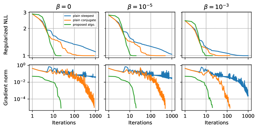
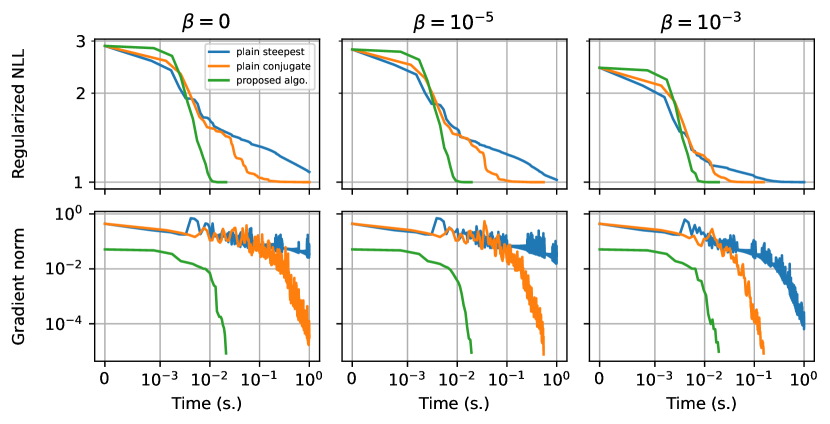
We begin with the minimization of the regularized NLL (26). data are drawn from a NC-MSG, i.e. . The parameter of this distribution is generated as explained in the introduction of this subsection with . Different parameters in (26) are considered: . The chosen regularization is the L2 penalty from Table I. When the NLL is the plain one, i.e. it is not regularized. We point out that, in this setup, the optimization goes well although the existence of a solution to this problem is not proven. When a solution to the minimization problem exists from Proposition 6. The minimization is performed with three different algorithms.
-
•
The plain conjugate gradient presented in [37]. It is a Riemannian conjugate gradient descent that uses a sum of three independent Riemannian metrics associated with the three parameters , , and . Thus, the corresponding Riemannian geometry is easier to derive but is not linked to the NC-MSG.
-
•
The plain steepest descent. It is similar to the plain conjugate gradient. Still, it only uses the gradient as a direction of descent (and not a linear combination with the direction of descent of the previous step).
- •
The results of this experiment are presented in Figures 1 and 3 in terms of iterations and computation time respectively. We observe that Algorithm 1 is much faster than the two others regardless of the parameter. Indeed, in the case , the Algorithm 1 is at least times faster than the plain steepest descent and times faster than the plain conjugate gradient. In the case of , Algorithm 1 is at least times faster than the plain steepest descent and times faster than the plain conjugate gradient. Furthermore, we observe these results are valid either in the number of iterations or in computation time. Indeed, the three considered algorithms have iterations with similar computational costs in . Thus, a reduction in the number of iterations results in a reduction in computation time.
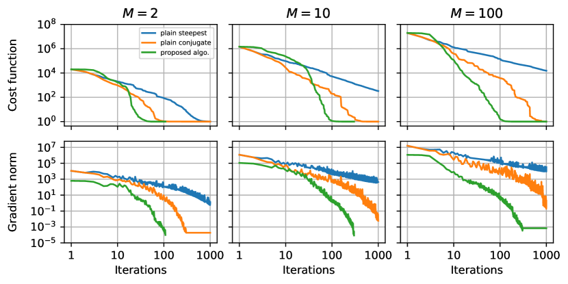
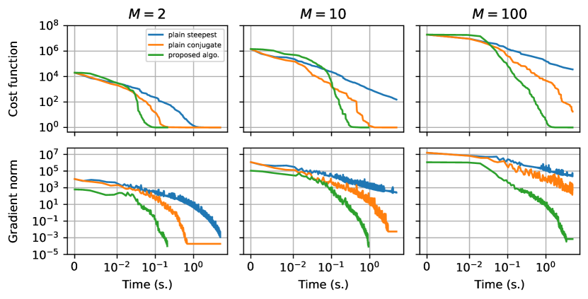
Then, a similar experiment is performed with the cost function (40) to compute the center of mass. parameters are generated as described in the introduction of Subsection VII-A with . The minimization is performed with the same optimization algorithms as previously: the plain steepest descent, the plain conjugate gradient, and Algorithm 1. The results of this experiment are presented in Figures 2 and 4 in terms of iterations and computation time, respectively.
We observe that Algorithm 1 is much faster than the two others regardless of . Indeed, when , Algorithm 1 converges in iterations whereas the plain conjugate gradient requires iterations and the plain steepest descent still has not converged after iterations. When , Algorithm 1 converges in less than iterations which is times faster than the plain conjugate gradient. It should be noted that the plain steepest descent has not converged after iterations in the cases . Once again, these results are valid either in the number of iterations or in computation time since the three considered algorithms have iterations with similar computational costs in . Hence, reducing the number of iterations implies a reduction in computation time.
The estimation error made by Algorithm 1 applied on the NLL (5) is studied with numerical experiments on simulated data. data are sampled from the NC-MSG (2). The parameter of this distribution is generated as presented in the introduction of Subsection VII-A with to have heterogeneous textures . The considered estimators for this numerical experiment are the following:
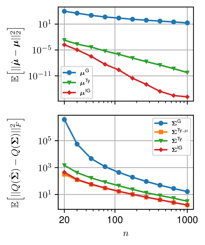
The estimation errors are measured with the Mean Squared Errors (MSE). These errors are computed as and , with , for the estimated location and the estimated scatter respectively, with Monte-Carlo. The MSE on the location and the scatter versus the number of samples are plotted in Figure 5. First, we observe in both figures that the Gaussian estimators have a high MSE. This shows the interest in considering robust estimators such as Tyler’s joint location-scatter matrix estimator or the proposed one when the textures are heterogeneous. Then, the proposed estimators realize a much lower MSE than Tyler’s joint location-scatter estimator. We can note that when enough samples are provided, the MSE on the location realized by the proposed estimator reaches the machine precision and is therefore negligible. Finally, we compare the performance of the proposed estimator with Tyler’s -estimator for the scatter estimation. Indeed, when the location is known, Tyler’s -estimator is the MLE of the NC-MSG (2). We observe that when enough samples are provided, the proposed estimator matches the MSE of Tyler’s -estimator. Overall, this experimental subsection illustrates the good performance of the proposed estimator when data are sampled from a NC-MSG (2).
VII-B Application
with
with
In the previous subsection, the different theoretical results derived in Sections from III to VI showed several interests in synthetic data. We now focus on applying a Nearest centroïd classifier on to real data using the estimation framework developed in Section V, the divergence and the Riemannian center of mass from Section VI as well as the optimization framework from Section IV. This classifier is compared with several other Nearest centroïd classifiers associated with different estimators and divergences.
To do so, we consider the dataset Breizhcrops [29]: a large-scale dataset of more than crop time series from the Sentinel-2 satellite to classify. More specifically, for each crop observations are measured over time. Each contains reflectance measurements of spectral bands. Then, these measurements are concatenated into one batch . Hence, we get one matrix per crop and each one belongs to an unknown class . These classes represent crop types such as nuts, barley, or wheat and are heavily imbalanced, i.e. some classes are much more represented than others. An example of a time series of meadows is presented in Figure 6. We apply a single preprocessing step: all the data are centered using the global mean. For simplicity, the matrix is noted in the following.
To classify these crops, we apply a Nearest centroïd classifier on descriptors. Indeed, the use of statistical descriptors is a classical procedure in machine learning as they are often more discriminative than raw data (see e.g. [19, 20]). Hence, this classification algorithm works in three steps.
-
1.
For each batch , a descriptor is computed, e.g. the parameter from the minimization of the regularized NLL (25).
-
2.
Then, on the training set, the center of mass of the descriptors of each class is computed. This center of mass is always computed by minimizing the variance associated with a divergence between descriptors. For example, the center of mass on is computed as in (40).
-
3.
Finally, on the test set, each descriptor is labeled with the class of the nearest center of mass with respect to the chosen divergence.
Six Nearest centroïd classifiers are considered, and they are grouped according to the divergence they use: the Euclidean distance, the symmetrized KL divergence between Gaussian distributions, or the symmetrized KL divergence (39) between NC-MSGs. For each divergence, several Nearest centroïd classifiers are derived using several estimators. These estimators correspond to different assumptions on the data.
Three Nearest centroïd classifiers rely on the Euclidean distance between matrices. Given two matrices and of the same size, the Euclidean distance is . The center of mass of a given set is the arithmetic mean which is the solution of . From this geometry, three Nearest centroïd classifiers are derived using three estimators: the batch itself , the sample mean and . The last two estimators correspond to the assumption that data follow a Gaussian distribution (either with the same scatter matrix for all batches or the same location).
Two Nearest centroïd classifiers rely on the symmetrized KL divergence between Gaussian distributions. Let . Given two pairs of parameters and , this divergence is given by where . The center of mass of is the solution of . Then, two Nearest centroïd classifiers are derived using two estimators: and the MLE of the Gaussian distribution .
Finally, the proposed Nearest centroïd classifier on relies on the symmetrized KL divergence (39) between NC-MSGs. The center of mass is computed as explained in the subsection VI-B and the estimation is described in Section V with the L2 penalty for the regularization. For initialization, we used the arithmetic mean, i.e. given a set of parameters , with , where , , and is the normalization function: , .
The data are divided into two sets: a training set and a test set with and batches respectively [29]. Among the six Nearest centroïd classifiers, only the one on has a hyperparameter which the parameter of the regularized NLL (25). Several values of are tested on a training set and a validation set, and both are subsets of the original training set. The performance is measured with the “F1 weighted” metric used in [29] and is plotted in Figure 7. The value of with the highest “F1 weighted” metric is . Hence, we use this value in the rest of the paper. Then, we propose an experiment to illustrate Proposition 8 on the invariance of the estimation of textures under rigid transformations. Indeed, we train the six Nearest centroïd classifiers on a subset of the original training set and apply them to the full test set with a rigid transformation. Thus, the more a Nearest centroïd classifier is robust to these rigid transformations, the better the “F1 weighted” metric. Given , three different rigid transformations are performed: transformation of the mean with for a given , rotation transformation with for a given skew-symmetric (hence ), and the joint mean and rotation transformation . It should be noted that at , the data are left unchanged. The results are presented in Figure 8.
The conclusions of these experiments are fourfold. First, the proposed Nearest centroïd classifier applies to large-scale datasets such as the Breizhcrops dataset. Second, the regularization proposed in Section V is important to get good classification performance. Indeed, we observe from Figure 7 that if is too small, then the “F1 weighted” metric becomes very low. Also, if is too large, then the “F1 weighted” metric also becomes very low. Third, using KL divergences and their associated centers of mass to classify estimators gives much better performance than the classical Euclidean distance. Indeed, even when data do not undergo rigid transformations, Nearest centroïd classifiers based on KL divergences outperform Euclidean Nearest centroïd classifiers in Figure 8. Fourth, considering NC-MSGs, as well as its KL divergence, instead of the Gaussian distribution, is interesting to classify time series especially when rigid transformations are applied to the data. Indeed, in Figure 8, we observe a large performance improvement when data are considered distributed from a NC-MSG and undergo rigid transformations.
VIII Conclusion
In this paper, we proposed a Riemannian gradient descent algorithm based on the Fisher-Rao information geometry of the NC-MSG. This algorithm is leveraged for two problems: parameter estimation and computation of centers of mass. The estimation problem of the NC-MSG is not straightforward. Indeed, a major issue is that the existence of a solution to the NLL minimization problem is not guaranteed. To overcome this issue, we proposed a class of regularized NLLs that make the trade-off between a white Gaussian distribution and the NC-MSG. These functions are guaranteed to have a minimum, and this result holds without conditions on the samples. Furthermore, we derived the KL divergence between NC-MSGs which enabled us to define the centers of mass of NC-MSGs as minimization problems. The latter is solved using the proposed Riemannian gradient descent. Simulations have shown that the proposed Riemannian gradient descent is fast on both minimization problems. Also, a Nearest centroïd classifier based on the KL divergence has been implemented. It has been applied on the large-scaled dataset Breizhcrops and showed robustness to transformations of the test set.
References
- [1] F. Kai-Tai and Z. Yao-Ting, Generalized multivariate analysis, vol. 19, Science Press Beijing and Springer-Verlag, Berlin, 1990.
- [2] R. A. Maronna, “Robust M-estimators of multivariate location and scatter,” Ann. Statist., vol. 4, no. 1, pp. 51–67, 01 1976.
- [3] E. Ollila, D. E. Tyler, V. Koivunen, and H. V. Poor, “Complex Elliptically Symmetric distributions: Survey, new results and applications,” IEEE Transactions on Signal Processing, vol. 60, no. 11, pp. 5597–5625, 2012.
- [4] A. Wiesel, “Unified framework to regularized covariance estimation in scaled gaussian models,” IEEE Transactions on Signal Processing, vol. 60, no. 1, pp. 29–38, 2011.
- [5] D. E. Tyler, “A distribution-free M-estimator of multivariate scatter,” Ann. Statist., vol. 15, no. 1, pp. 234–251, 03 1987.
- [6] E. Conte, A. De Maio, and G. Ricci, “Recursive estimation of the covariance matrix of a compound-gaussian process and its application to adaptive cfar detection,” IEEE Transactions on signal processing, vol. 50, no. 8, pp. 1908–1915, 2002.
- [7] F. Pascal, P. Forster, J.-P. Ovarlez, and Larzabal P., “Performance analysis of covariance matrix estimates in impulsive noise,” IEEE Transactions on signal processing, vol. 56, no. 6, pp. 2206–2217, 2008.
- [8] G. Frahm and U. Jaekel, “Tyler’s m-estimator, random matrix theory, and generalized elliptical distributions with applications to finance,” Random Matrix Theory, and Generalized Elliptical Distributions with Applications to Finance (October 21, 2008), 2008.
- [9] T. Zhang, X. Cheng, and A. Singer, “Marčenko–Pastur law for Tyler’s m-estimator,” Journal of Multivariate Analysis, vol. 149, pp. 114–123, 2016.
- [10] P.-A. Absil, R. Mahony, and R. Sepulchre, Optimization Algorithms on Matrix Manifolds, Princeton University Press, Princeton, NJ, USA, 2008.
- [11] N. Boumal, “An introduction to optimization on smooth manifolds,” in Cambridge University Press, March 2023.
- [12] F. Nielsen, “The many faces of information geometry,” Not. Am. Math. Soc, vol. 69, pp. 36–45, 2022.
- [13] F. Pascal, Y. Chitour, and Y. Quek, “Generalized robust shrinkage estimator and its application to stap detection problem,” IEEE Transactions on Signal Processing, vol. 62, no. 21, pp. 5640–5651, 2014.
- [14] Y. Sun, P. Babu, and D. P. Palomar, “Regularized Tyler’s scatter estimator: Existence, uniqueness, and algorithms,” IEEE Transactions on Signal Processing, vol. 62, no. 19, pp. 5143–5156, 2014.
- [15] E. Ollila and D. E Tyler, “Regularized -estimators of scatter matrix,” IEEE Transactions on Signal Processing, vol. 62, no. 22, pp. 6059–6070, 2014.
- [16] Y. Sun, P. Babu, and D. P. Palomar, “Regularized robust estimation of mean and covariance matrix under heavy-tailed distributions,” IEEE Transactions on Signal Processing, vol. 63, no. 12, pp. 3096–3109, 2015.
- [17] A. Breloy, E. Ollila, and F. Pascal, “Spectral shrinkage of Tyler’s -estimator of covariance matrix,” in 2019 IEEE 8th International Workshop on Computational Advances in Multi-Sensor Adaptive Processing (CAMSAP). IEEE, 2019, pp. 535–538.
- [18] M. Yi and D. E. Tyler, “Shrinking the covariance matrix using convex penalties on the matrix-log transformation,” Journal of Computational and Graphical Statistics, vol. 30, no. 2, pp. 442–451, 2020.
- [19] A. Barachant, S. Bonnet, M. Congedo, and C. Jutten, “Multiclass brain–computer interface classification by riemannian geometry,” IEEE Transactions on Biomedical Engineering, vol. 59, no. 4, pp. 920–928, 2012.
- [20] O. Tuzel, F. Porikli, and P. Meer, “Human detection via classification on riemannian manifolds,” in 2007 IEEE Conference on Computer Vision and Pattern Recognition, 2007, pp. 1–8.
- [21] O. Tuzel, F. Porikli, and P. Meer, “Pedestrian detection via classification on riemannian manifolds,” IEEE transactions on pattern analysis and machine intelligence, vol. 30, no. 10, pp. 1713–1727, 2008.
- [22] P. Formont, J.-P. Ovarlez, and F. Pascal, “On the use of matrix information geometry for polarimetric sar image classification,” in Matrix Information Geometry, pp. 257–276. Springer, 2013.
- [23] H. Karcher, “Riemannian center of mass and mollifier smoothing,” Communications on Pure and Applied Mathematics, vol. 30, no. 5, pp. 509–541, 1977.
- [24] M. Arnaudon, F. Barbaresco, and L. Yang, Medians and Means in Riemannian Geometry: Existence, Uniqueness and Computation, pp. 169–197, Springer Berlin Heidelberg, Berlin, Heidelberg, 2013.
- [25] S. Chevallier, E. K. Kalunga, Q. Barthélemy, and E. Monacelli, “Review of riemannian distances and divergences, applied to ssvep-based bci,” Neuroinformatics, vol. 19, no. 1, pp. 93–106, 2021.
- [26] M. Calvo and J. M. Oller, “An explicit solution of information geodesic equations for the multivariate normal model,” Statistics and Risk Modeling, vol. 9, no. 1-2, pp. 119–138, 1991.
- [27] M. Tang, Y. Rong, J. Zhou, and X. Li, “Information geometric approach to multisensor estimation fusion,” IEEE Transactions on Signal Processing, vol. 67, no. 2, pp. 279–292, 2019.
- [28] A. Collas, F. Bouchard, G. Ginolhac, A. Breloy, C. Ren, and J.-P. Ovarlez, “On the use of geodesic triangles between gaussian distributions for classification problems,” in ICASSP 2022 - 2022 IEEE International Conference on Acoustics, Speech and Signal Processing (ICASSP), 2022, pp. 5697–5701.
- [29] M. Rußwurm, C. Pelletier, M. Zollner, S. Lefèvre, and M. Körner, “Breizhcrops: A time series dataset for crop type mapping,” International Archives of the Photogrammetry, Remote Sensing and Spatial Information Sciences ISPRS (2020), 2020.
- [30] E. Ollila, D. E. Tyler, V. Koivunen, and H. V. Poor, “Compound-gaussian clutter modeling with an inverse gaussian texture distribution,” IEEE Signal Processing Letters, vol. 19, no. 12, pp. 876–879, 2012.
- [31] F. Pascal, Y. Chitour, J.-P. Ovarlez, P. Forster, and Larzabal P., “Covariance structure maximum-likelihood estimates in compound gaussian noise: Existence and algorithm analysis,” IEEE Transactions on Signal Processing, vol. 56, no. 1, pp. 34–48, 2007.
- [32] A. Breloy, G. Ginolhac, A. Renaux, and F. Bouchard, “Intrinsic Cramér–Rao bounds for scatter and shape matrices estimation in CES distributions,” IEEE Signal Processing Letters, vol. 26, no. 2, pp. 262–266, 2019.
- [33] F. Bouchard, A. Mian, J. Zhou, S. Said, G. Ginolhac, and Y. Berthoumieu, “Riemannian geometry for compound Gaussian distributions: application to recursive change detection,” Signal Processing, 2020.
- [34] A. Wiesel and T. Zhang, Structured robust covariance estimation, Now Foundations and Trends, 2015.
- [35] Y. Sun, P. Babu, and D. P. Palomar, “Robust estimation of structured covariance matrix for heavy-tailed elliptical distributions,” IEEE Transactions on Signal Processing, vol. 64, no. 14, pp. 3576–3590, 2016.
- [36] B. Meriaux, C. Ren, M. N. El Korso, A. Breloy, and P. Forster, “Robust estimation of structured scatter matrices in (mis) matched models,” Signal Processing, vol. 165, pp. 163–174, 2019.
- [37] A. Collas, F. Bouchard, A. Breloy, C. Ren, G. Ginolhac, and J.-P. Ovarlez, “A Tyler-type estimator of location and scatter leveraging riemannian optimization”,” in Acoustics, Speech and Signal Processing (ICASSP), 2021 IEEE International Conference on, Toronto, Canada. June 2021, 2021.
- [38] S. Amari, Information Geometry and Its Applications, Springer Publishing Company, Incorporated, 1st edition, 2016.
- [39] L. T. Skovgaard, “A Riemannian geometry of the multivariate Normal model,” Scandinavian Journal of Statistics, vol. 11, no. 4, pp. 211–223, 1984.
- [40] M. Pilté and F. Barbaresco, “Tracking quality monitoring based on information geometry and geodesic shooting,” in 2016 17th International Radar Symposium (IRS), 2016, pp. 1–6.
- [41] D. Maclaurin, D. Duvenaud, and Adams R.P., “Autograd: Effortless gradients in pure numpy,” AutoML workshop ICML, 2015.
- [42] J. Bradbury, R. Frostig, P. Hawkins, M.J. Johnson, C. Leary, D. Maclaurin, G. Necula, A. Paszke, J. VanderPlas, S. Wanderman-Milne, and Q. Zhang, “JAX: composable transformations of Python+NumPy programs,” in ., 2018.
- [43] A. Wiesel, “Geodesic convexity and covariance estimation,” IEEE Transactions on Signal Processing, vol. 60, no. 12, pp. 6182–6189, 2012.
- [44] Esa Ollila, Daniel P. Palomar, and Frédéric Pascal, “Shrinking the eigenvalues of m-estimators of covariance matrix,” IEEE Transactions on Signal Processing, vol. 69, pp. 256–269, 2021.
- [45] M. Moakher, “A differential geometric approach to the geometric mean of symmetric positive-definite matrices,” SIAM Journal on Matrix Analysis and Applications, vol. 26, no. 3, pp. 735–747, 2005.
- [46] F. Mezzadri, “How to generate random matrices from the classical compact groups,” Notices of the AMS, 2006.
- [47] P. Virtanen, R. Gommers, T. E. Oliphant, M. Haberland, et al., and SciPy 1.0 Contributors, “SciPy 1.0: Fundamental Algorithms for Scientific Computing in Python,” Nature Methods, vol. 17, pp. 261–272, 2020.
- [48] S. Smith, “Covariance, subspace, and intrinsic Cramér-Rao bounds,” Signal Processing, IEEE Transactions on, vol. 53, pp. 1610–1630, 06 2005.
- [49] F. Bouchard, A. Breloy, G. Ginolhac, A. Renaux, and F. Pascal, “A Riemannian framework for low-rank structured elliptical models,” IEEE Transactions on Signal Processing, vol. 69, no. 3, pp. 1185–1199, 2021.
Supplementary Material:
Riemannian optimization for a non-centered mixture of scaled Gaussian distributions
Antoine Collas, Arnaud Breloy, Chengfang Ren, Guillaume Ginolhac, Jean-Philippe Ovarlez
-A Proof of Proposition 1: Fisher Information Metric
First, we recall the definition of the FIM. See [48] for an in-depth presentation. Let be data points. Assuming that the underlying distribution admits a p.d.f., the corresponding NLL, denoted , maps parameters belonging to the parameter space of the p.d.f., denoted , onto . By denoting the tangent space of at , and under conditions of regularity of , the FIM is defined as
To derive the FIM of the mixture of scaled Gaussians given in Proposition 1, we recall classical formulas for the Gaussian distribution. The NLL at and associated to one data point is (neglecting terms not depending on )
| (41) |
Since is an open set in the vector space , the tangent space of at is . Finally, , the FIM of the Gaussian distribution associated to the NLL (41) is [39]
| (42) |
Then, we derive the FIM associated with the NLL of the mixture of scaled Gaussian distributions (5). We begin by writing (5) as a sum of Gaussian NLL (41). Indeed, , we have
where . Thus, , , and following the reasoning of [49, Proposition 6] and [33, Proposition 3.1], the FIM of the mixture of scaled Gaussian is expressed as a sum of FIM of the Gaussian distribution (42)
In the following, the -th components of and are denoted and respectively. Therefore, the directional derivative of the function is
Thus, we get
Since , we have . Thus, the last two terms of the last equation cancel, and the expression of the FIM from Proposition 1 is obtained
It should be noted that this formula defines an inner product on if a transpose is added to . Thus, is extended as presented in Proposition 1.
-B Proof of Proposition 2: orthogonal projection on
First of all, the ambient space defined in (14) is decomposed into two complementary subspaces
| (43) |
where is the tangent space at defined in (15) and is the orthogonal complement
| (44) |
It can be checked that this orthogonal complement is
| (45) |
where is the set of skew-symmetric matrices. Indeed, the elements of (45) verify the definition (44) and . Using the equations (43) and (45), the orthogonal projection of onto is
where and have to be determined. Furthermore, with , we must have
This induces that
where . Thus, we get the orthogonal projection from Proposition 2.
-C Proof of Proposition 3: Levi Civita connection on
First of all, the FIM defined in Proposition 1 is rewritten with a function . Indeed, let and be smooth vector fields on , the function is defined as
| (46) |
This function is of primary importance for the development of the Levi Civita connection.
We briefly introduce the Levi-Civita connection. The general theory of it can be found in [10, Ch. 5]. The Levi-Civita connection, simply denoted , is characterized by the Koszul formula. Let be a smooth vector field on , in our case the Koszul formula writes
| (47) |
where is the directional derivative of the function . We begin by computing :
Since the objective is to identify using (47) and the FIM from Proposition 1, the last equation needs to be rewritten. To do so, the following two terms are rewritten
and, since
Hence, we get the equation (48). We then compute in equation (49). Using (48) and (49), we calculate the right-hand side of the Koszul formula (47) in equation (50). By identification of the Koszul formula (47) and orthogonal projection onto the tangent space, we get the Levi Civita connection from the Proposition 3.
| (48) | ||||
| (49) | ||||
| (50) | ||||
-D Proof of Proposition 4: Riemannian gradient on
Let be a smooth function and be a point in . We present the correspondence between the Euclidean gradient of (which can be computed using automatic differentiation libraries such as Autograd [41] and JAX [42]) and the Riemannian gradient associated with the FIM defined in Proposition 1. The Euclidean gradient of at is defined as the unique element in such that
Then, the Riemannian gradient is defined as the unique element in such that
Hence, , we get that
where
To get the Riemannian gradient, it remains to project into the tangent space using the orthogonal projection . Thus, we get the Riemannian gradient from the Proposition 4.
-E Proof of Proposition 5: a second order retraction on
| (46) | ||||
where .
| (47) | ||||
Let , and where is to be defined. We denote where is defined in Proposition 5, i.e.
where , is defined as .
The objective is to prove that is a second-order retraction on . The different properties of the definition of a second-order retraction are verified in the following; see [10, Ch. 4 and 5] for a complete definition.
First of all, we define such that is a valid retraction. Indeed, must respect some constraints of positivity,
| (51) | |||
| (52) |
where for , means is positive definite and for , means the components of are strictly positive. Of course, (51) and (52) are not necessarily respected depending on the value of . To define the value of such that (51) and (52) are respected, we begin by studying the eigenvalues of the left side of (51). To do so, let be the smallest eigenvalue of and be the left side of (51). Thus, we get that
| (53) |
A sufficient condition to satisfy (51) is that the right side of (53) is strictly positive. This is achieved whenever is in where is defined as followed
-
•
if , and ,
-
•
if , for , otherwise.
Lets denote the minimum value coordinate of by . Using the same reasoning as before, one can show that whenever is in , where is defined in the following, (52) is satisfied.
-
•
If , and .
-
•
If , for , otherwise.
Hence, we get such that , .
Then, to be a second-order retraction, it remains to check that the three following properties are respected,
| (54) |
where and is the Levi-Civita connection defined in Proposition 3. The first property is easily verified. In the rest of the proof, the following notations are used: , and .
We verify the second property of (54) which is . It is readily check that and . It remains to verify that . Computing the derivative of (defined in Proposition 3) at a point , we get that
| (55) |
where . Using this derivative and the constraints and , the desired property is derived
It remains to check the third condition of (54). Using the first two conditions of (54), we get that if and only if
where, , . It is readily checked that the first two conditions are met. Thus, only the third condition remains to be verified. To do so, we differentiate (55) to get the second derivative of in equation (46). Using this derivative and the constraints and , the expression of is derived in the equation (47). Using the linearity of the projection , (47) implies that
Finally, one can check that , . Hence, we get the desired expression
which completes the proof.