Quantitative theory of backscattering in topological HgTe and (Hg,Mn)Te quantum wells:
acceptor states, Kondo effect, precessional dephasing, and bound magnetic polaron

Abstract

We present the theory and numerical evaluations of the backscattering rate determined by acceptor holes or Mn spins in HgTe and (Hg,Mn)Te quantum wells in the quantum spin Hall regime. The role of anisotropic $s$–$p$ and $sp$–$d$ exchange interactions, Kondo coupling, Luttinger liquid effects, precessional dephasing, and bound magnetic polarons is quantified. The determined magnitude and temperature dependence of conductance are in accord with experimental results for HgTe and (Hg,Mn)Te quantum wells.

I Introduction

The experimental discovery of the quantum spin Hall effect (QSHE) in HgTe quantum wells (QWs) König et al. (2007) provided experimental support for the seminal theoretical predictions about the topological protection Kane and Mele (2005); Bernevig et al. (2006) and opened prospects for electron transport without scattering backward, the capability of interest for energy-efficient and decoherence-free classical and quantum devices. However, in studied two-dimensional (2D) topological systems, such as aforementioned HgTe QWs König et al. (2007); Roth et al. (2009) and 1T’-WTe₂ 2D monolayers Fei et al. (2017); Wu et al. (2018), the two-terminal conductance approaches the quantized value $2e^{2}/h$ only in mesoscopic samples, shorter than 10 and 0.1 $\mu$m, respectively, without much improvement on cooling below 50 mK.

Understandably, the origin of processes accounting for the unanticipatedly short topological protection length has attracted a considerable attention. In 2D topological materials, electrons reside in counter-propagating Kramers degenerate helical states adjacent to sample edges. Furthermore, the direction of electron momentum determines the spin orientation. Therefore, mechanisms leading to electron backscattering must contain ingredients that break both time-reversal and spin-rotation symmetry. As reviewed recently Hsu et al. (2021); Yevtushenko and Yudson (2022), previous theories considering backscattering in the linear response regime can be costed into three categories. The first of them contains approaches associating those ingredients to the presence of electron-electron interactions within the helical channels Ström et al. (2010); Crépin et al. (2012); Lezmy et al. (2012); Pikulin and Hyart (2014); Wang et al. (2017); Novelli et al. (2019). The second class of models considers the effects of external spins coming from extrinsic defects Maciejko et al. (2009); Altshuler et al. (2013); Väyrynen et al. (2014), magnetic impurities Hattori (2011); Tanaka et al. (2011); Cheianov and Glazman (2013); Kimme et al. (2016); Kurilovich et al. (2019); Yevtushenko and Yudson (2022) or nuclear spins Lunde and Platero (2013); Hsu et al. (2017). Finally, the influence of random magnetic fluxes has been examined Delplace et al. (2012). It can be argued that the abundance of theoretical proposals reflects difficulties in assessing magnitudes of material parameters entering into particular models, precluding a conclusive comparison of the theory to experimental results.

This paper, supporting and extending the companion report Dietl (2023a), presents theory and provides numerical evaluations of conductance in the regime of the quantum spin Hall effect (QSHE) in HgTe König et al. (2007) and (Hg,Mn)Te quantum wells Shamim et al. (2020), considering holes localized on acceptors as a source of backscattering. We have quantitatively determined acceptor energies, the Coulomb gap, exchange coupling between edge electrons and acceptor holes, Kondo temperatures for both acceptor holes and Mn spins, spin-flip and backscattering rates in strong and weak coupling regimes, and effects of bound magnetic polarons. In addition to the Kondo effect discussed already in the context of backscattering Maciejko et al. (2009); Altshuler et al. (2013), we incorporate into our approach spin-nonconserving anisotropic components of the exchange coupling, allowing for backscattering even in the spin-momentum locking case Tanaka et al. (2011); Altshuler et al. (2013); Lunde and Platero (2013); Kimme et al. (2016); Yevtushenko and Yudson (2022).

Our theoretical and numerical results substantiate the main conclusion of the companion paper Dietl (2023a) that the value of the exchange interaction between edge electrons and acceptor holes is large enough to drive the system to the strong coupling regime of the Kondo effect, where the spin-flip scattering rate attains the unitary limit. Together with the demonstrated sizable exchange anisotropy, the unitary scattering rate explains the observed topological protection length in HgTe QWs in the Ohmic conductivity regime König et al. (2007); Bendias et al. (2018); Lunczer et al. (2019) and the corresponding temperature dependence of conductance, if the influence of Luttinger liquid effects upon the anisotropic exchange are taken into account Väyrynen et al. (2016). A key aspect of our approach is the observation that the acceptor concentration is known experimentally, as it determines hole density in undoped QWs and the gate voltage range separating the electron and hole transport in a given QW. In this way our theory does not involve any fitting parameters. Accordingly, the quantitative agreement with experimental data appears meaningful.

In contrast to occupied acceptor dopants, our results indicate that no Kondo effect is expected for impurities with open $d$ or $f$ shells in dilute magnetic semiconductors (DMSs), at least for typical values of antiferromagnetic $sp$–$df$ exchange integrals. Furthermore, for magnetic ions with orbital momentum $L=0$, such as Mn²⁺, anisotropic components of the exchange coupling to edge states vanish, suggesting a minor role of Mn spins in backscattering. Nevertheless, we suggest that backscattering by a dense bath of interacting Mn spins can operate, as for the motionally-narrowed precessional spin-dephasing process, the constraint of local spin momentum conservation is relaxed. At the same time, we show that the formation of bound magnetic polarons by acceptor holes reduces the role of the Kondo effect, the observation elucidating the origin of the recovery of quantized conductance at low temperatures in (Hg,Mn)Te QWs Shamim et al. (2021).

II Theoretical results

II.1 Quantum-well band states

A starting point of our theory is the eight-band Kohn–Luttinger Hamiltonian with boundary conditions previously used to obtain the subband structure in HgTe QWs Novik et al. (2005) and the four–band model developed for determining, in the axial approximation, acceptor levels in GaAs QWs Fraizzoli and Pasquarello (1991). Within that approximation, discussed in Sec. II.1, and in the absence of the impurity potential, the eight relevant electron wave functions $\psi_{i}$ can be taken in the form,

$$\psi_{i}^{(m_{i})}(\rho,\varphi,z)=h_{i}^{(m_{i})}(\rho,\varphi)f_{i}(z)u_{i},$$ (1)

where $m_{i}$ is the integer orbital quantum number corresponding to the $z$-component of the orbital momentum $l_{z}$ of the envelope function $h_{i}$; $\rho$, $\varphi$, and $z$ denote the electron position in the cylindrical coordinates with $z$ along the growth direction; $u_{i}\equiv u_{j,jz}$ is the set of the Kohn–Luttinger amplitudes for particular angular momenta $j$ and its $z$-component $j_{z}$: $s_{1/2,1/2}$, $s_{1/2,-1/2}$, $p_{3/2,3/2}$, $p_{3/2,1/2}$, $p_{3/2,-1/2}$, $p_{3/2,-3/2}$, $p_{1/2,1/2}$, and $p_{1/2,-1/2}$ Novik et al. (2005), whereas the envelope functions $h_{i}^{(m_{i})}(\rho,\phi)$ and $f_{i}(z)$ are given by,

$$h_{i}^{(m_{i})}(\rho,\varphi)=N_{\text{o}}i^{|m_{i}|}\exp(im_{i}\varphi)J_{|m_{i}|}(k\rho),$$ (2)

where $N_{\text{o}}$ is a normalization factor. The Hamiltonian in question can be diagonalized by taking $m_{i}=m$ for $i=1$, 4, and 7; $m_{i}=m+1$ for $i=2$, 5, and 8; $m_{i}=m-1$ for $i=3$, and $m_{i}=m+2$ for $i=6$, where $m$ is an integer and $J_{|m_{i}|}(k\rho)$ is the Bessel function; $k$ is a module of the in-plane wavevector, and

$$f_{i}(z)=(1/\sqrt{L_{z}})\sum_{n=-n_{\text{max}}}^{n_{\text{max}}}c^{(i)}_{n}\exp(2\pi inz/L_{z}),$$ (3)

where $L_{z}$ is the total thickness of the structure, including the two Cd_0.7Hg_0.3Te barriers and HgTe QW, assumed here as $L_{z}=60$ nm + $d_{\text{QW}}$; the expansion coefficients $c^{(i)}_{n}$ are to be determined by a diagonalization procedure; $n_{\text{max}}=50$ ensures an appropriate numerical convergence, as discussed in Sec. II.4. As seen by inspection, each of the eight components $\psi_{i}^{(m_{i})}(\rho,\varphi,z)$ and, hence, the total wave function corresponds to the same value of the total angular momentum $F_{z}=l_{z}+j_{z}=m+1/2$, meaning that the operator $F_{z}$ commutes with the eight-bands’ axial Hamiltonian.

We adopt the identical values of low-temperature ${\vec{k}}\cdot{\vec{p}}$ parameters, as in Ref. Novik et al. (2005), except for the Luttinger $\kappa$ that we assume to be the same in the barriers and QW. In this way, no Rashba-like splitting occurs in symmetric QWs. Computations have been performed assuming the absence of strain. Its role is discussed in Sec. II.3.

Figures 1(a,b) in the companion paper Dietl (2023a) present QW subband dispersions $E(k)$ for $d_{\text{QW}}=6$ and 8 nm. The magnitudes of $f_{i}(z)$ for $d_{\text{QW}}=8$ nm and $k=0$ are shown in Fig. 1. A character of their inversion symmetry ($z\rightarrow-z$) plays an essential role in the anisotropy of the electron-hole exchange interaction, as discussed in Sec. II.6.

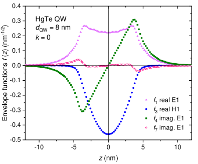
Figure 1: Envelope functions $f_{1}(z)$, $f_{3}(z)$, $f_{4}(z)$, and $f_{7}(z)$ at $k=0$ for E1 and H1 subbands in HgTe quatum well of 8 nm-width. The envelopes $f_{3}$ and $f_{6}=f_{3}$ correspond to the Kramer’s pair for the H1 subband, whereas $f_{1}$, $f_{4}$, $f_{7}$ and $f_{2}=-f_{1}$, $f_{5}=-f_{4}$, $f_{8}=f_{7}$ for the E1 subband with a relative weight 53.6, 45.9, and 0.5%, respectively. As seen, the values of $f_{j}$ are either real and symmetric or imaginary and antisymmetric in respect to the QW center at $z=0$.

II.2 Axial approximation

Figure 2 shows subband dispersions $E({\vec{k}})$ computed without and with the axial approximation for HgTe QW thicknesses 6 and 8  nm. A slight overestimation of the indirect gap by the axial approximation is visible for $d_{QW}=8$ nm. Since, however, the energy differences between ${\vec{k}}\|\langle 10\rangle$ and ${\vec{k}}\|\langle 11\rangle$ near valence band top are significantly smaller than the acceptor binding energies in Fig. 1(c) of the companion paper Dietl (2023a), the axial approximation holds.

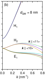
Figure 2: Verification of axial approximation. Subband dispersions for a HgTe QW of the thickness $d_{\text{QW}}=6$ nm (a) and $8$ nm (b) computed for ${\vec{k}}\|\langle 11\rangle$ (dashed lines), ${\vec{k}}\|\langle 10\rangle$ (dotted lines) and within the axial approximation (solid lines). Character of particular subbands at $k=0$ is also marked.

II.3 Strain effects

We use a conventional sign definition of biaxial epitaxial strain Bir (1974); O’Reilly (1989); Dietl and Ohno (2014), i.e., a positive value of $\epsilon_{xx}=\epsilon_{yy}$ corresponds to QW under the tensile strain. In particular, in the case of HgTe QW, $\epsilon_{xx}=0.31$% corresponds to strain for a CdTe substrate, whereas a Cd_1-xZn_xTe substrate generates a compressive strain Leubner et al. (2016), $\epsilon_{xx}<0$. The evolution of the QW band structure with biaxial strain is shown in Fig. 3 for HgTe QW of the thickness $d_{\text{QW}}=6$ nm and $\epsilon_{xx}=0.31$%, 0, and $-0.31$%.

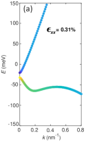
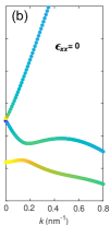
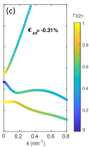
Figure 3: Effects of biaxial strain on band dispersion in HgTe QWs. (a) $\epsilon_{xx}=0.31$% (CdTe substrate); (b) $\epsilon_{xx}=0$; (c) $\epsilon_{xx}=-0.31$%. Colors describe the participation of the $p_{3/2,\pm 3/2}$ Kohn-Luttinger amplitude in the electronic wave function; HgTe QW thickness $d_{\text{QW}}=6$ nm.

The strain, and also temperature, shift the QW thickness corresponding to the topological phase transition ($E_{\text{g}}=0$), but the overall band picture remains intact, in agreement with previous conclusions Novik et al. (2005); Leubner et al. (2016); Kadykov et al. (2018).

II.4 Determination of acceptor level energies

To determine energies of levels brought about by charge dopants, we supplement the Hamiltonian by the Coulomb potential,

$$V(r)=-Ze^{2}/4\pi\epsilon_{0}\epsilon r,$$ (4)

and by the potential of image charges in the barriers Fraizzoli and Pasquarello (1991), for which the dielectric constant is $\epsilon_{\text{b}}=(1-x_{\text{b}})\epsilon+x_{\text{b}}\epsilon_{\text{e}}$, where in our case $\epsilon=19.5$, $\epsilon_{\text{e}}=10.5$, and $x_{\text{b}}=0.7$. We neglect central cell corrections and the image charge in the gate metal, which is typically more than 100 nm apart.

Furthermore, we replace the Bessel function $J_{|m_{j}|}(k\rho)$ in Eq. 2 by

$$J_{|m_{i}|}(k\rho)\rightarrow\rho^{|m_{i}|}\sum_{l=1}^{l_{\text{max}}}d^{(i)}_{l}\exp(-\rho/a_{l}),$$ (5)

where the coefficients $d^{(i)}_{l}$ are to be determined by the diagonalization procedure for a given set of ${a_{l}}$ values. We take ${a_{l}}$ as a geometrical series with a common ratio of $r=1.5$ and, for a typical number of exponential functions $l_{\text{max}}=15$, the starting value of $a_{1}=0.5$ nm. Since, the exponential functions with real exponents are not orthogonal, a generalized eigenvalue solver has been employed to obtain electronic energies. At the same time, the participation number serves to evaluate an effective in-plane localization radius $a^{*}$.

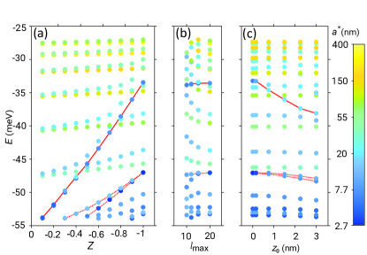
Figure 4: Example of the identification of acceptor levels $E_{3/2}$ $(m=1)$ degenerate with the QW band states. (a) Energy levels $E$ as a function of the center charge $Z$. (b) $E$ as a function of the number of exponential functions $l_{\text{max}}$ in Eq. 5 and for $n_{\text{max}}=25$ (Eq. 3). (c) $E$ as a function of the distance of acceptor to QW center $z_{0}$ for $l_{\text{max}}=15$ and $n_{\text{max}}=50$. Color scale depicts the magnitude of an effective in-plane Bohr radius $a^{*}$ in the logarithmic scale. Red solid lines show the ground state $E_{3/2}$ acceptor level; dotted lines represent examples of acceptor excited states. HgTe QW thickness $d_{\text{QW}}=6$ nm; no strain.

The presence of the impurity potential breaks the degeneracy of the states with respect to the quantum number $m$. However, due to time–reversal symmetry, the impurity levels remain at least doubly degenerate. The use of exponential functions (Eq. 5) is suitable for determining the localized levels but not for oscillating extended states. Accordingly, the values of band energies do not converge with increasing $l_{\text{max}}$.

In our case, identifying acceptor levels that overlap with the continuum of band states appears difficult Buczko and Bassani (1992); Zholudev et al. (2020). Figure 4 depicts level energies determined for $m=1$ in a HgTe QW with $d_{\text{QW}}=6$ nm. As shown, the magnitude of $a^{*}$, and the evolution of the level energies with $Z$ [Fig. (a)], $l_{\text{max}}$ [Fig. 4(b)], and with the acceptor location of the QW center [Fig. 4(c)] unambiguously tell the band and resonant impurity states. According to the result presented in the companion paper Dietl (2023a), the ground state corresponds to $m=0$ or $m=-1$, and is predominately built of the $p_{3/2,\pm 1/2}$ and $s_{1/2,\pm 1/2}$ Kohn-Luttinger amplitudes. Its energy is referred to as $E_{1/2}$.

II.5 Coulomb gap

The Efros-Shklovskii Coulomb gap Shklovskii and Efros (1984) of the width $E_{\text{C}}$ reaching 10 meV was observed in a single-layer of 1T’-WTe₂ with different coverage of surface by potassium Song et al. (2018). Furthermore, numerical simulations revealed the presence of the Coulomb gap for resonant donor states in HgSe:Fe Wilamowski et al. (1990).

In terms of 2D DOS of the acceptor band taken as $\nu_{2}=N_{\text{a}}/E_{\text{b}}$, where $E_{\text{b}}$ is the acceptor bandwidth Shklovskii and Efros (1984),

$$E_{\text{C}}=2\nu_{2}e^{4}/(4\pi\epsilon_{0}\epsilon)^{2}.$$ (6)

In the case of QWs, a non-zero $E_{\text{b}}$ originates from a dependence of the binding energy on the distance between the impurity and QW center. Figure 1(c) in the companion paper Dietl (2023a) shows this effect for acceptors in HgTe QWs, and demonstrates that the bandwidth extends down to a side maximum of the valence band characterized by a heavy mass. For a HgTe QW with $d_{\text{QW}}=8$ nm, where $E_{\text{b}}\simeq 20$ meV and the QW dielectric constant $\epsilon=19.5$, we obtain the value of $E_{\text{C}}=0.51$ meV for $N_{\text{a}}=10^{11}$ cm^-2. The magnitude of $E_{\text{C}}$ sets the temperature scale above which conductance quantization deteriorates and hole mobility $\mu_{h}$ decreases for QWs at the topological phase transition. Thus, the Coulomb gap model explains the stability of the QSHE up to 100 K in WTe₂ monolayers Wu et al. (2018), where – as mentioned above – $E_{\text{C}}$ attains 10 meV Song et al. (2018).

II.6 Electron-hole spin exchange

Taking into account previous insight that flip-flop transitions conserving total spin of edge electrons and, thus, due to spin-momentum locking edge current Tanaka et al. (2011), we are interested in determining the degree $r$ of axial symmetry breaking by the QW edge for the exchange interaction between topological edge electrons and acceptor holes in HgTe QWs. One of possible mechanisms could be kinetic exchange discussed in semiconductors in the context of $p$–$d$ coupling Kacman (2001) and the Kondo effect in quantum dots Pustilnik and Glazman (2004). However, we demonstrate here that the Bir–Pikus theory, originally developed for excitons Bir (1974), and later extended to the case of exchange coupling between band electrons and acceptor holes in bulk semiconductors Śliwa and Dietl (2008), satisfactorily explains the experimental results for HgTe QWs.

The wave function of helical states at the edge along the $x$-direction assumes the form,

$$\psi_{e}^{(+)}(\vec{r}) = \frac{\exp(ikx)}{\sqrt{L_{x}}}[f_{1}(\vec{\mathtt{r}})u_{1}+f_{4}(\vec{\mathtt{r}})u_{4}+f_{3}(\vec{\mathtt{r}})u_{3}];$$ (7)

$$\psi_{e}^{(-)}(\vec{r}) = {\mathcal{T}}\psi_{e}^{(+)}(\vec{r}),$$ (8)

where $L_{x}$ is the edge length; $f_{i}$ are electron envelope functions that depend on $\vec{\mathtt{r}}=(y,z)$; $u_{i}$ are the relevant Luttinger-Kohn amplitudes, and ${\mathcal{T}}=-i\sigma_{y}K$ is a time reversal operator. Similarly, for the acceptor ground state,

$$\psi_{h}^{(+)}(\vec{r}) = {\mathcal{C}}[F_{1h}(\vec{r})u_{1}+F_{4h}(\vec{r})u_{4}];$$ (9)

$$\psi_{h}^{(-)}(\vec{r}) = {\mathcal{T}}\psi_{h}^{(+)}(\vec{r}),$$ (10)

where ${\mathcal{C}}=\sigma_{y}K$ is a charge conjugation operator transforming the acceptor wave function from the electron representation, employed in previous sections for the determination of electronic states, to the hole representation relevant here. In contrast, in the case of edge states we consider electrons and, thus, the electron representation for the Fermi level both above and below the Dirac point.

With these wave functions we determine a long-range contribution to the electron-hole exchange Bir (1974); Śliwa and Dietl (2008). This interaction is nonlocal and represented, in the case under consideration, by the matrix elements,

$${\cal{H}}_{eh}^{\sigma,\sigma\prime;\mu,\mu\prime}=-\frac{\hbar^{2}}{m_{0}^{2}}\sum_{\alpha,\beta}\int d\vec{r}_{1}d\vec{r}_{2}\partial^{2}_{r_{1}^{(\alpha)}r_{2}^{(\beta)}}V(r_{12})$$

$$\cdot\langle\psi_{e}^{\sigma}(\vec{r}_{1})|p_{\alpha}|\psi_{h}^{\mu}(\vec{(}r_{1})\rangle_{\Omega}\langle\psi_{e}^{\sigma\prime}(\vec{r}_{2})|p_{\beta}|\psi_{h}^{\mu\prime}(\vec{(}r_{2})\rangle_{\Omega},$$ (11)

where $\sigma$ and $\mu=\pm$; $\alpha,\beta=x,y,z$; ${\vec{r}}_{12}=\vec{r}_{1}-\vec{r}_{2}$. Furthermore, in accord with the effective mass theory, internal matrix elements containing momentum operators $p_{\alpha}$ and $p_{\beta}$ are over the elementary cell volume $\Omega$ and involve the amplitudes $u_{i}$, whereas the envelope functions are assumed constant within this volume. As seen, non-vanishing matrix elements correspond to coupling of $s$-type and $p$-type edge states with $p$-type and $s$-type acceptor states, respectively. Neglecting electrostatic image charges, the Coulomb energy has a standard form,

$$V(r_{12})=\frac{e^{2}}{4\pi\epsilon_{0}\epsilon r_{12}}.$$ (12)

It is convenient to present a spatial function in the Coulomb term as a sum of the local monopole and non-local dipole components,

$$\partial^{2}_{r_{1}^{(\alpha)}r_{1}^{(\beta)}}r_{12}^{-1}=-\frac{4\pi}{3}\delta_{\alpha\beta}\delta(\vec{r}_{12})$$

$$-\frac{(r_{12})^{2}\delta_{\alpha\beta}-3\vec{r}_{12}^{(\alpha)}\vec{r}_{12}^{(\beta)}}{r_{12}^{5}}.$$ (13)

In the case of electrons at the bottom of the conduction band and holes localized on acceptor impurities in bulk zinc-blende semiconductors, the exchange coupling has a scalar (Heisenberg) form, ${\cal{H}}_{eh}=-{\cal{J}}\vec{s}\cdot\vec{j}$, where $j=3/2$ and ${\cal{J}}<0$ Śliwa and Dietl (2008). Since the QW and the edge break rotational symmetry, we expect, in the presence of intratomic spin-orbit coupling, a nonscalar form of the exchange interaction,

$${\cal{H}}_{eh}=-\sum_{\alpha,\beta}s_{\alpha}{\cal{J}}^{(\alpha,\beta)}j_{\beta},$$ (14)

where ${\cal{J}}^{(\alpha,\beta)}$ is a real tensor and, in a standard notation, ${\cal{J}}_{\alpha}={\cal{J}}^{(\alpha,\alpha)}$, and if $\alpha\neq\beta$, ${\cal{J}}_{\alpha,\beta}^{(s)}=({\cal{J}}^{(\alpha,\beta)}+{\cal{J}}^{(\beta,\alpha)}/2$; $D_{\alpha}=\sum_{\beta,\gamma}\epsilon_{\alpha\beta\gamma}{\cal{J}}^{(\beta,\gamma)}/2$, where $D_{\alpha}$ are vector components of the Dzyaloshinskii-Moriya (DM) contribution and $\epsilon_{\alpha\beta\gamma}$ is the antisymmetric Levi-Civita tensor.

By comparing matrix elements of Hamiltonians given in Eqs. 11 and 14, considering both monopole and dipole contributions of the long-range electron-hole exchange interaction (Eq. 13), and taking into account that ${\cal{H}}_{eh}=-{\cal{H}}_{ee}$, we arrive to final forms of non-zero exchange tensor components and a spin-independent part of the Fock energy $\Delta_{eh}$,

$${\cal{J}}_{x,y}=A\left(\frac{16\pi}{9}{\cal{M}}_{21}+\frac{4}{3}{\cal{M}}_{31}-3{\cal{M}}_{52}\pm{\cal{M}}_{51}\right);$$ (15)

$${\cal{J}}_{z}=A\left[\frac{8\pi}{9}({\cal{M}}_{11}-3{\cal{M}}_{12})+\frac{5}{3}{\cal{M}}_{41}+{\cal{M}}_{42}+2\sqrt{3}i{\cal{M}}_{63}\right];$$ (16)

$${\cal{J}}_{yz}^{(s)}=iA\left(\frac{8\sqrt{3}\pi}{9}{\cal{M}}_{13}-\frac{\sqrt{3}}{3}{\cal{M}}_{43}-\sqrt{3}{\cal{M}}_{53}\right);$$ (17)

$${\cal{D}}_{x}=-iA\left(\frac{8\sqrt{3}\pi}{9}{\cal{M}}_{13}+\frac{\sqrt{3}}{3}{\cal{M}}_{43}+\sqrt{3}{\cal{M}}_{53}\right);$$ (18)

$$\Delta_{eh}=A\left[\frac{2\pi}{3}({-\cal{M}}_{11}+{\cal{M}}_{12})-\frac{1}{4}{\cal{M}}_{41}-\frac{1}{4}{\cal{M}}_{42}-\frac{\sqrt{3}i}{2}{\cal{M}}_{63}\right].$$ (19)

In the above formulae the prefactor $A$ contains information about the strength of the Coulomb interaction and $\vec{k}\cdot\vec{p}$ coupling,

$$A=\frac{e^{2}}{4\pi\epsilon_{0}\epsilon}\frac{P^{2}}{E_{eh}^{2}L_{x}},$$ (20)

where $P$ is Kane’s $s$-$p$ momentum matrix element and $E_{he}$ is the energy distance between hole and electron states in question.

Particular matrix elements ${\cal{M}}_{ij}$ are given by

$${\cal{M}}_{ij}=\int d\vec{r}_{1}d\vec{r}_{2}g_{i}(\vec{r}_{1},\vec{r}_{2})O_{j}(\vec{r}_{1},\vec{r}_{2}),$$ (21)

where

$$g_{1}({\vec{r}_{1}},{\vec{r}_{2}}) = \delta(\vec{r}_{12});$$ (22)

$$g_{2}({\vec{r}_{1}},{\vec{r}_{2}}) = \cos[k(x_{1}+x_{2})]\delta(\vec{r}_{12});$$ (23)

$$g_{3}({\vec{r}_{1}},{\vec{r}_{2}}) = \cos[k(x_{1}+x_{2})](r_{12}^{2}-3z_{12}^{2})/r_{12}^{5};$$ (24)

$$g_{4}({\vec{r}_{1}},{\vec{r}_{2}}) = \cos[k(x_{1}-x_{2})](r_{12}^{2}-3z_{12}^{2})/r_{12}^{5};$$ (25)

$$g_{5}({\vec{r}_{1}},{\vec{r}_{2}}) = \cos[k(x_{1}+x_{2})](x_{12}^{2}-y_{12}^{2})/r_{12}^{5};$$ (26)

$$g_{6}({\vec{r}_{1}},{\vec{r}_{2}}) = \sin[k(x_{1}-x_{2})]x_{12}z_{12}/r_{12}^{5},$$ (27)

Overlap functions between edge-electron and acceptor-hole envelopes read

$$O_{1}(\vec{r}_{1},\vec{r}_{2})=[f_{4}(\vec{\mathtt{r}}_{1})F_{1h}(\vec{r}_{1})-f_{1}(\vec{\mathtt{r}}_{1})F_{4h}(\vec{r}_{1})]$$

$$\cdot[f_{4}(\vec{\mathtt{r}}_{2})F_{1h}(\vec{r}_{2})-f_{1}(\vec{\mathtt{r}}_{2})F_{4h}(\vec{r}_{2})];$$ (28)

$$O_{2}(\vec{r}_{1},\vec{r}_{2})=f_{3}(\vec{\mathtt{r}}_{1})F_{1h}(\vec{r}_{1})f_{3}(\vec{\mathtt{r}}_{2})F_{1h}(\vec{r}_{2});$$ (29)

$$O_{3}(\vec{r}_{1},\vec{r}_{2})=f_{3}(\vec{\mathtt{r}}_{1})F_{1h}(\vec{r}_{1})$$

$$\cdot[f_{4}(\vec{\mathtt{r}}_{2})F_{1h}(\vec{r}_{2})-f_{1}(\vec{\mathtt{r}}_{2})F_{4h}(\vec{r}_{2})],$$ (30)

where for the adopted phase convention, in accord with the results presented in Fig. 1, $f_{1}(\vec{\mathtt{r}}),f_{3}(\vec{\mathtt{r}})$, and $F_{1h}(\vec{r})$ are real, $f_{3}(\vec{\mathtt{r}})$ is negative, whereas $f_{4}(\vec{\mathtt{r}})$ and $F_{4h}(\vec{r})$ are imaginary and change sign as a function of $z$.

Inspection of the above equations shows that exchange integrals ${\cal{J}}_{\alpha}$ are negative, implying antiferromagnetic coupling between edge electrons and localized holes, which allows for the Kondo coupling. At the same time, the presence of terms breaking the axial symmetry leads to spin non-conserving transitions ($r\neq 0$) and, hence to net backscattering of edge electrons. The off-diagonal exchange tensor components ${\cal{J}}_{yz}^{(s)}$ and ${\cal{D}}_{x}$ are non-zero for both monopole and dipole coupling but only if the inversion symmetry is broken, i.e., the acceptor resides away of the QW center, so that the hole envelope functions $F_{1h}$ and $F_{4h}(\vec{r})$ cease to be symmetric and antisymmetric with respect to $z=0$, respectively. The presence of such terms was noted for dipole interactions of edge electrons with nuclear spins Lunde and Platero (2013) and for the Heisenberg interaction with magnetic impurities Kimme et al. (2016). However, in our case, even if inversion symmetry is maintained and, moreover, even if the $s$-type component in the hole wave function is negligible ($F_{1h}=0$), spin non-conserving transitions are still allowed by the edge-induced breaking of the axial symmetry, leading to ${\cal{J}}_{x}\neq{\cal{J}}_{y}$ in the dipole contribution.

For numerical evaluations, guided by theoretical results obtained for the edge states Lunde and Platero (2013); Papaj et al. (2016); Krishtopenko and Teppe (2018) and our data presented in Secs. II.1 and II.4, we assume the electron and hole envelope functions in an approximate form,

$$f_{1}(y,z)=2e_{s}\exp(-y/b)\Theta(y)\cos(\pi z/d_{\text{QW}})\Theta(d_{\text{QW}}/2-|z|)/(bd_{\text{QW}})^{1/2};$$ (31)

$$f_{4}(y,z)=2ie_{p}\exp(-y/b)\Theta(y)\sin(2\pi z/d_{\text{QW}})\Theta(d_{\text{QW}}/2-|z|)/(bd_{\text{QW}})^{1/2};$$ (32)

$$f_{3}(y,z)=2e_{H}\exp(-y/b)\Theta(y)\cos(\pi z/d_{\text{QW}})\Theta(d_{\text{QW}}/2-|z|)/(bd_{\text{QW}})^{1/2};$$ (33)

$$F_{1h}({\vec{r}})=h_{s}\exp[-(x^{2}+(y-y_{\text{m}})^{2})^{1/2}/a^{*}]\Theta(y)\cos[\pi(z-z_{\text{m}})/d_{\text{QW}}]\Theta(d_{\text{QW}}/2-|z|)/N_{\text{o}};$$ (34)

$$F_{4h}({\vec{r}})=ih_{p}\exp[-(x^{2}+(y-y_{\text{m}})^{2})^{1/2}/a^{*}]\Theta(y)\sin[2\pi(z-z_{\text{m}})/d_{\text{QW}}]\Theta(d_{\text{QW}}/2-|z|)/N_{\text{o}}.$$ (35)

Here $b$ describes the penetration length of the edge electron wave function into the QW; $\Theta(x)$ is the Heaviside step function, $y_{\text{m}}$ and $z_{\text{m}}$ are distances of a maximum of the hole wave function from the sample edge located at $y=0$ and the QW center residing at $z=0$, respectively, and $N_{\text{o}}$ is an in-plane normalization factor. We note that one expects $|z_{\text{m}}|<d_{\text{QW}}/2$ even for acceptors localized outside the QW, $|z_{0}|>d{\text{QW}}/2$. Making use of previous results Lunde and Platero (2013) as well as of our data presented in Secs. II.1 and II.4, we take $e_{s}=0.26$; $e_{p}=0.24$; $e_{H}=-0.93$; $h_{s}=0.31$; and $h_{p}=0.92$; as the factors determining the participation of particular orbital components in the total electron and hole wave functions. Furthermore, the computations have been performed for $d_{\text{QW}}=8$ nm and $a^{*}=5$ nm. A Monte Carlo method has been used to evaluate six dimensional integrals. Such a method minimizes systematic errors but necessarily leads to a statistical scatter of the results. The chosen number of evaluation points insures that the accuracy of the obtained data is better than one sigma.

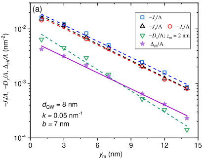
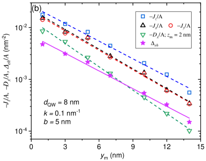
Figure 5: Computed values (points) of exchange integrals ${\cal{J}}_{\alpha}/A$, the Dzyaloshinskii-Moriya energy $D_{x}/A$, and the spin-independent term $\Delta_{eh}$ for coupling between edge electrons and acceptor holes in topological HgTe QW, plotted as a function of the distance $y_{\text{m}}$ between the acceptor wave function maximum and the edge; (a) the electron wavevector $k=0.05$ nm^-1 and the penetration of helical state into the QW, $b=7$ nm; (b) $k=0.1$ nm^-1 $b=5$ nm. The material constant $A$ is defined in Eq. 20. Lines are linear fits to the computed points.

Figure 5 presents exchange tensor components as a function of $y_{\text{m}}$ for two values of $k=0.05$ and 0.1 nm^-1 and the corresponding magnitudes of $b=7$ and 5 nm, respectively Lunde and Platero (2013); Papaj et al. (2016); Krishtopenko and Teppe (2018). As could be expected for the exchange interaction, ${\cal{J}}_{\alpha}/A$ exponentially decay with $y_{\text{m}}$ but, not surprisingly, this decay is weaker for $r_{xy}=[(2({\cal{J}}_{x}-{\cal{J}}_{y})/({\cal{J}}_{x}+{\cal{J}}_{y})]^{2}$, as shown in Fig. 6. The magnitude of $r_{xy}$ is independent of $A$ and unaffected by a shift of the acceptor away from the QW center. However, for $z_{\text{m}}\neq 0$, other axial symmetry breaking terms appear, ${\cal{J}}_{yz}$ and $D_{x}$, where $|{\cal{J}}_{yz}|\ll|D_{x}|$, and, for $z_{\text{m}}=d_{\text{QW}}/4$, $r_{Dx}=[(3D_{x}/({\cal{J}}_{x}+{\cal{J}}_{y}+{\cal{J}}_{z})]^{2}\gg r_{xy}$, as depicted in Fig. 6. In the subsequent two sections, the obtained values of ${\cal{J}}_{\alpha}/A$ and $r_{i}$ serve to estimate the magnitude of Kondo temperature and of the backscattering rate.

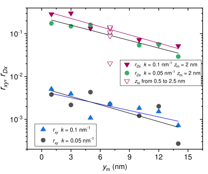
Figure 6: Computed magnitudes of exchange anisotropy ratio $r_{xy}=[(2({\cal{J}}_{x}-{\cal{J}}_{y})/({\cal{{\cal{J}}}}_{x}+{\cal{J}}_{y})]^{2}$ and $r_{Dx}=[(3D_{x}/({\cal{J}}_{x}+{\cal{J}}_{y}+{\cal{J}}_{z})]^{2}$ for edge electrons in topological HgTe QWs as a function of the distance $y_{\text{m}}$ between the acceptor wave function maximum and the edge, obtained for ${\cal{J}}_{\alpha}$ and $D_{x}$ values display in Fig. 5; the results are for two electron wavevectors $k=0.05$ and $0.1$ nm^-1, for which the penetration of helical state into the QW $b=7$ and $5$ nm, respectively. In the case of $r_{Dx}$, the distance between the QW center and the wave function maximum $z_{\text{m}}=2$ nm (full points) or varies between 0.5 and 2.5 nm with 0.5 nm step (empty triangles); $k=0.1$ nm^-1; $r_{Dx}(z_{\text{m}}=0)=0)$. Lines are linear fits to the computed points.

Finally, we comment on the spin-independent part of the Fock energy $\Delta_{eh}$, which together with Hartree terms originating from acceptor, edge, and gate charges, contribute to a self-consistent potential in the edge region, whose determination is beyond scope of the present work. Nevertheless, to have an idea about the energy scale involved, we evaluate a contribution to one-electron energy resulting from the Fock term in a self-consistent way making use of Eqs. 19 and 20, and summing up over all holes with the areal density $N_{h}$,

$$E_{eh}^{(\text{F})}=\left[\frac{e^{2}N_{\text{a}}P^{2}}{4\pi\epsilon_{0}\epsilon}\int dy|f(y)|^{2}\Delta_{eh}(y)/A\right]^{1/3}.$$ (36)

where the dependence $\Delta_{eh}(y)/A$ is displayed in Fig. 5 for two values of $k$ and $b$. Assuming $f(y)=\exp(-b/y)/\sqrt{b/2}$; $N_{\text{a}}=0.5\cdot 10^{11}$ cm^-2; $P=8.28\cdot 10^{-8}$ eVcm, and $\epsilon=19.5$ we obtain $E_{eh}^{(\text{F})}=4.8$ and $4.4$ meV for $b=5$ and 7 nm, respectively.

II.7 Kondo temperatures for acceptor holes and Mn spins

II.7.1 Acceptor holes

A Kondo collective state results from antiferromagnetic exchange coupling of Fermi liquid with a single spin localized at ${\vec{R}}_{i}$. An antiferromagnetic electron-hole interaction leads also to the Kondo effect, as in the electron picture it corresponds to antiferromagnetic coupling of a surplus localized electron with the electron Fermi liquid. To estimate an order of magnitude of Kondo temperatures $T_{\text{K}}$, we use a time-honored expression Daybell and Steyert (1968) costed to the form,

$$k_{\text{B}}T_{\text{K}}\simeq W\exp[-1/(L^{d}\nu_{d}|{\mathcal{J}}_{d}|)],$$ (37)

where $W$ is a energy width of carrier-containing states; $\nu_{d}$ is the carrier DOS per spin, and ${\cal{J}}_{d}$ represents the exchange energy of the antiferromagnetic interaction between spins of one carrier and a single localized paramagnetic center. Both $\nu_{d}$ and ${\mathcal{J}}_{d}$ correspond to values at the Fermi level, and depend on the dimensionality $d$ of the Fermi liquid residing in a structure of the volume $L^{d}$.

For the case under consideration, $\nu_{1}=1/2\pi\hbar v_{\text{F}}$, where $v_{\text{F}}=4\cdot 10^{5}$ m/s Lunde and Platero (2013); Papaj et al. (2016); Krishtopenko and Teppe (2018), and ${\cal{J}}_{1}=({\cal{J}}_{x}+{\cal{J}}_{y})/2$ at given $y_{\text{m}}$, $k$, $b$, and the energy of the acceptor hole with respect to the Fermi level, $E_{eh}$. Furthermore, together with $P$ and $\epsilon$ values quoted in previous sections, we take $W$ as a half of the bandgap, i.e., 15 meV for $T_{\text{K}}$ estimations.

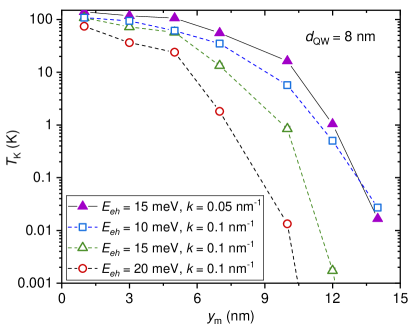
Figure 7: Calculated magnitudes (points) of Kondo temperatures, obtained for ${\cal{J}}_{x}$ and ${\cal{J}}_{y}$ values display in Fig. 5, for edge electrons in HgTe QWs containing holes bound to acceptors as a function of the distance $y_{\text{m}}$ between the acceptor wave function maximum and the edge calculated for various values of the electron-hole energy interval $E_{eh}$; full points: electron wavevector $k=0.05$ nm^-1 and the penetration of helical state into the QW, $b=7$ nm; open points: $k=0.1$ nm^-1 $b=5$ nm. Lines connect calculated points.

Several important conclusions emerge from $T_{\text{K}}$ magnitudes presented in Fig. 7 as a function of $y_{\text{m}}$. First, for acceptor holes localized close to the edge, $y_{\text{m}}<b$, $T_{\text{K}}$ reaches 100 K, indicating that the Kondo physics is relevant for the system of edge electrons and acceptor holes, making competing effects, such as exchange interactions between hole spins, irrelevant. Second, due to the exponential dependencies of $T_{\text{K}}$ on ${\cal{J}}_{\alpha}$ and ${\cal{J}}_{\alpha}$ on $y_{\text{m}}$ there is a sharp cut-off $y{\text{c}}$, beyond which strong coupling of holes and electrons vanishes. The magnitude of $y{\text{c}}$ depends on $b$ and $E_{eh}$, that is, also on the position of the Fermi level in the acceptor band. Third, a broad distribution of $T_{\text{K}}$ values means that at any experimentally relevant temperature, coupling of edge electrons and holes corresponds to a superposition of weak and strong coupling limits, including the crossover between them occurring at $T\simeq T_{\text{K}}$.

II.7.2 Kondo effect for Mn spins

For comparison, we evaluate also the magnitude of Kondo temperature for a transition metal impurity, such Mn, residing at $\vec{R}_{i}$ in a HgTe bulk sample or in a topological edge channel. A $p$-type part of the Bloch function is relevant, as the $p$–$d$ exchange integral $\beta$ is antiferromagnetic, whereas the $s$–$d$ integral $\alpha$ is ferromagnetic Dietl (1994). Accordingly, ${\cal{J}}_{d}$ appearing in Eq. 37 for $T_{\text{K}}$, can be written in a form,

$${\cal{J}}_{d}=\beta[|F_{3/2}(\vec{R}_{i})|^{2}+|F_{1/2}(\vec{R}_{i})|^{2}/3],$$ (38)

where $F_{jz}$ are envelope functions accompanying the Kohn-Luttinger amplitudes $p_{3/2,j_{z}}$. We see that an upper limit for the bulk case is ${\cal{J}}_{3}=\beta/{\cal{V}}$, where ${\cal{V}}$ is the sample volume. Similarly, for a Mn ion localized at a topological channel, where $\vec{R}_{i}=(x,0,0)$ and, thus, ${\cal{J}}_{1}=4\beta/(L_{x}bd_{\text{QW}})$.

Now, knowing that $N_{0}\beta=-0.7$ eV in HgTe Autieri et al. (2021), where $N_{0}=1.49\cdot 10^{22}$ cm^-3 is the cation concentration, we are in position to evaluate a lower limit of the exponent $w$ in Eq. 37 for $T_{\text{K}}$. For the bulk case, where $\nu_{3}=k_{\text{F}}m^{*}/2\pi^{2}\hbar^{2}$ and $m^{*}=0.45m_{0}$ Jȩdrzejczak and Dietl (1976), $w=-1.1\cdot 10^{3}$ for the hole concentration $p=10^{16}$ cm^-3 and $w=-49$ for $p=10^{20}$ cm^-3, implying $T_{\text{K}}\sim 10^{-20}$ K. For topological edge channels in HgTe QWs, taking $b=5$ nm, $d_{\text{QW}}=8$ nm, and $v_{\text{F}}=4\cdot 10^{5}$ m/s, we obtain $w=-350$.

Hence, it appears that for standard values of the $sp$-$df$ exchange integrals, no presence of the Kondo effect is expected for spins tightly localized on $d$ or $f$ shells in semiconductors with magnetic ions. The same conclusion holds for nuclear spins for which the hyperfine coupling constant is at least four orders of magnitude smaller compared to $N_{0}\beta$.

III Comparison to experimental results

III.1 Topological protection length: acceptor holes and Mn spins

III.1.1 Acceptor holes

Our approach to charge transport by topological edge channels in quantum spin Hall (QSH) materials is built on several pillars put previously forward by others, discussed in the companion paper Dietl (2023a), or elaborated in previous sections of the present paper. First, charge dopants determine pertinent properties of 2D topological systems, including the dependence of carrier density on the gate voltage $V_{\text{g}}$ and the magnitudes of electron and hole mobilities. Second, owing to a dependence of the dopant binding energy on the position with respect to the QW center, the acceptors form a band extending over the whole bandgap. The associated Coulomb gap in the acceptor hole spectrum controls a contribution of QW states to charge transport in the QSH regime Dietl (2023a). Third, due to a close energetic proximity, exchange interactions between edge channel electrons and acceptor holes are strong enough to bring the system to the Kondo regime (Sec. II.7). As known, spin-dephasing rate reaches a unitary limit in that regime Maciejko et al. (2009); Micklitz et al. (2006). Fourth, since the magnitude of Kondo temperature $T_{\text{K}}$ exponentially depends on the distance of the acceptor hole to the edge and on the energy interval to the Fermi level, $T_{\text{K}}$ values show a broad distribution covering the whole experimentally relevant temperature range (Sec. II.7). This effect determines also a spacial region from which acceptor holes contribute to spin-dephasing. Fifth, it has been emphasized by many authors Tanaka et al. (2011); Altshuler et al. (2013); Lunde and Platero (2013); Eriksson (2013); Kimme et al. (2016) that because of spin-momentum locking, spin-conserving transitions imply momentum conservation, i.e., no net backscattering between helical channels in 2D topological insulators. However, spin-orbit interactions can result in spin-nonconserving processes described by nonscalar terms in the exchange coupling between edge electrons and paramagnetic centers Tanaka et al. (2011); Altshuler et al. (2013); Lunde and Platero (2013); Eriksson (2013); Kimme et al. (2016). The magnitude of such terms has been determined in Sec. II.6 for the case of QW holes bound to acceptor impurities.

We are interested in the topological protection length $L_{\text{p}}=v_{\text{F}}/\gamma_{\text{b}}$, where $\gamma_{\text{b}}$ is a backscattering rate for helical states. To see its relation to the two terminal conductance $G=1/R$, we note that $R$ is non-zero due to the quantum contact resistance $R_{\text{q}}=h/2e^{2}$ and the backscattering term which, according to the Einstein relation, is given by $R_{\text{b}}=L^{2-d}\gamma_{\text{b}}(2e^{2}\nu_{d}v_{\text{F}}^{2}/d)^{-1}$. Hence, in our case, where $d=1$,

$$G=(2e^{2}/h)(1+L_{x}/L_{\text{p}})^{-1}.$$ (39)

To evaluate $\gamma_{\text{b}}$ we recall a form of the carrier spin-dephasing rate in Kondo systems,

$$\gamma_{s}=Cn_{S}f(T/T_{\text{K}})/2\pi\hbar\nu_{d},$$ (40)

where $C$ is a numerical coefficient close to one; $n_{S}$ in the concentration of magnetic impurities and $f(x)$ is a function obtained by the numerical renormalization group approach Micklitz et al. (2006); Costi et al. (2009) that is more accurate than the original Nagaoka-Suhl resummation result, $f(x)=a/[a+\ln^{2}(T/T_{\text{K}})]$, where $a=3\pi^{2}/4$. In either case, $f(0)=0$; $f(1)\simeq 1$, and $f(10)\simeq 0.6$.

It has been previously noted that compared to $\gamma_{s}$, the backscattering rate for helical channels is reduced by the exchange anisotropy ratio $r$, $\gamma_{b}=r\gamma_{s}$ Tanaka et al. (2011); Lunde and Platero (2013); Kimme et al. (2016). Thus, inverse $L_{\text{p}}$ can be written in an appealingly simple form Dietl (2023a),

$$L_{\text{p}}^{-1}(T)=\sum_{i}r^{(i)}f(T/T_{\text{K}}^{(i)})/L_{x},$$ (41)

where the summation is over all QW holes bound to acceptors for a given $V_{\text{g}}$. As shown in Fig. 6, the $r$ value is not universal, but varies with the hole position in respect to the edge and QW center, $y_{\text{m}}$ and $z_{\text{m}}$, respectively, and to a lesser degree with $k$ and $b$. Similarly, according to results presented in Fig. 7, the $T_{\text{K}}$ magnitude strongly depends on $y_{\text{m}}$ and also on $E_{eh}$ that is controlled by the Fermi level position and $z_{0}$, the distance of the acceptor to the QW center, as shown in Fig. 1 of Ref. Dietl, 2023a. However, just to see whether we are on the right track, we take the areal hole density as $N_{h}=0.5\cdot 10^{11}$ cm^-2, an average value of $r^{(i)}$ as $r_{Dx}(z_{\text{m}}=2$ nm) = 0.13 (see, Fig. 6), the cut-off length beyond which strong coupling of holes and electrons tends to vanish $y_{\text{c}}=2b=10$ nm (see, Fig. 7), and an average value of $f(T/T_{\text{K}})=0.4$. These numbers lead to the linear density $n_{h}=5/\mu$m of holes participating in backscattering and $L_{\text{p}}=4$ $\mu$m, the order of magnitude consistent with experimental findings König et al. (2007); Lunczer et al. (2019); Majewicz (2019). A small number of scattering centers has several important consequences, as discussed below.

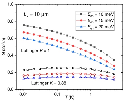
Figure 8: Configurationally averaged two-terminal conductance $G$ in the units $2e^{2}/h$ vs. temperature for a HgTe QW of the thickness $d_{\text{QW}}=8$ nm and length $L_{x}=10$ $\mu$m computed for various energy distance of the Fermi level to the acceptor state $E_{eh}$; $k=0.1$ nm^-1 $b=5$ nm; full points: no Luttinger liquid effects ($K=1$); empty points: Luttinger liquid effects taken into account ($K=0.88$). Lines connect calculated points.

Figure 8 shows the temperature dependence of two-terminal conductance $G$, as defined in Eq. 39, for a 10 $\mu$m long device of HgTe QW. The values of $G$ have been obtained by integrating $L_{\text{p}}^{-1}$ given in Eq. 41 in the $xy$ plane with the areal density of acceptor holes $N_{h}=0.5\cdot 10^{11}$ cm^-2. The latter changes with the gate voltage and its overall magnitude vary from sample to sample. However, typically, the gate voltage width corresponding to the gap region, $\Delta V_{\text{g}}$, implies the total acceptor density of the order of $10^{11}$ cm^-2. The theoretical results are presented for three values of $E_{eh}$ and $L_{x}$. As $r(y)$, we have used the values fitted to $r_{Dx}(z_{\text{m}}=2$ nm) in Fig. 6. Similarly, $T_{\text{K}}(y)$ is determined from fitted values of ${\cal{J}}_{x}$ and ${\cal{J}}_{y}$ shown by dashed lines in Fig. 5. Finally, the function $f(T/T_{\text{K}})$ has been obtained from the data in Fig. 3 for $d=1$ of Ref. Micklitz et al., 2006 and from the proposed there high-temperature extrapolation.

A number of worthwhile conclusions can be drawn from data in Fig. 8. In particular, lowering of temperature eliminates from backscattering spin centers with $T_{\text{K}}>T$, so that $L_{\text{p}}$ and $G$ are seen to steadily increase on cooling. However, the predicted recovery of $G=2e^{2}/h$ at $T\rightarrow 0$ Maciejko et al. (2009); Väyrynen et al. (2016) is not found, as at any temperature there are centers far away from the channel for which $T_{\text{K}}\gtrsim T$. Nevertheless our results are not in accord with experimental findings in a sense that no systematic increase of $G$ on decreasing $T$ has been observed. This disagreement can point to the onset of localization, predicted for disordered Kondo systems Altshuler et al. (2013) or to the presence of Tomonaga-Luttinger effects Maciejko et al. (2009); Väyrynen et al. (2016). In has been shown Väyrynen et al. (2016) that renormalization group equations combining Kondo and carrier correlation phenomena imply a growth of the exchange anisotropy ratio $r$ with lowering temperature down to $T^{*}$ according to,

$$r(T)=r(W)(W/k_{\text{B}}T)^{2}(1-K),$$ (42)

with

$$k_{\text{B}}T^{*}=W\left[\frac{L_{x}\nu_{1}|{\cal{J}}_{1}|}{\sqrt{2}(1-K)}\right]^{1/(1-K)},$$ (43)

where the Luttinger parameter $K<1$ for interacting 1D systems. As shown in Fig. 8, incorporation of $r(T)$ into our theory makes $G$ virtually independent of $T$ for a rather moderate interaction magnitude $K=0.88$. It should be, however, noted that at any temperature only a part of acceptor holes resides sufficiently far from the edge to satisfy the condition $T>T^{*}$.

Up to now, we have discussed configuration-averaged behavior of an acceptors’ containing system. However, a small number of acceptor holes involved in micron-size samples means that $G(V_{\text{g}})$ will show strong mesoscopic-like conductance fluctuations, as observed König et al. (2007); Grabecki et al. (2013); Shamim et al. (2021); Bubis et al. (2021). Furthermore, if at given $V_{\text{g}}$, acceptor holes close to the edge dominate for which $T_{\text{K}}>T$, $f(T/T_{\text{K}})$ will increase and, hence, $G(T)$ decrease with temperature. By contrast, for distance acceptors $T_{\text{K}}<T$, so that a falling down of $f(T/T_{\text{K}})$ with $T$ works together with the Tomonaga-Luttinger effects to result in an increase of $G(T)$ on heating. Such changes in sign of $dG(T)/dT$ with $V_{\text{g}}$ have been observed experimentally, though regions with $dG(T)/dT>0$ appear to prevail Bubis et al. (2021). According to Eq. 41 and many experimental observations, conductance quantization can be improved in short samples, $L_{x}\ll L_{\text{p}}$. However, a small number of relevant acceptors results in substantial conductance fluctuations. Charge traps biding two electrons in a singlet state might reduce backscattering and ensure pinning of the Fermi level in the QW band gap.

III.1.2 Backscattering by Mn spins and precessional spin dephasing

As there are typically $10^{4}$ more Mn spins with $S=5/2$ in Hg_0.99Mn_0.01Te compared with the number of acceptor holes, a question arises about the role of Mn-induced backscattering of edge electrons. As the number of Mn ions in the edge region is also much larger than the number of edge electrons, we consider Mn spins in a continuous and classical approximation. Such an approximation is not only employed in the description of static and dynamic spintronics functionalities of ferromagnetic metals but has also been found versatile and quantitatively accurate in the case of bound magnetic polarons and single quantum dot electrons immersed in a nuclear spin bath in semiconductors Dietl (2015) as well as when considering carrier-mediated ferromagnetism in DMSs Dietl and Ohno (2014). Within this approach, it is convenient to expand local magnetization $\vec{M}(\vec{r})$ into a Fourier series,

$$\vec{M}(\vec{r})=\sum_{\vec{q}}\vec{\eta}_{\vec{q}}\exp(i\vec{q}\cdot\vec{r})/\sqrt{{\cal{V}}}.$$ (44)

For a uniform distribution of Mn ions over the volume ${\cal{V}}$ encompassing the QW and under thermal equilibrium conditions, the fluctuation-dissipation theorem implies,

$$\langle\eta^{(\alpha)}_{\vec{q}}\eta^{(\beta)}_{\vec{q\prime}}\rangle=k_{\text{B}}T\chi_{\alpha,\beta}(\vec{q})\delta_{\vec{q},\vec{-q}\prime},$$ (45)

where in cubic systems and in the absence of a magnetic field, the magnetic susceptibility tensor $\chi_{\alpha,\beta}(\vec{q})=\delta_{\alpha,\beta}\chi_{\text{Mn}}(q,T)$. We then apply a standard weak-coupling procedure (Fermi’s golden rule) for spin-flip transitions between 1D helical states, $\psi_{e}^{(+)}(\vec{r})\rightarrow\psi_{e}^{(-)}(\vec{r})$, and adopt the form of $\psi_{e}^{(\pm)}(\vec{r})$ given in Eq. 8. The scattering rate becomes,

$$\gamma_{\text{Mn}}=\frac{k_{\text{B}}T\chi_{\text{Mn}}(T)}{2\hbar^{2}g^{2}\mu_{\text{B}}^{2}v_{\text{F}}}\int d\vec{\mathtt{r}}[\alpha^{2}|f_{1}(\vec{\mathtt{r}})|^{4}+\beta^{2}(|f_{3}(\vec{\mathtt{r}})|^{4}+|f_{4}(\vec{\mathtt{r}})|^{4})],$$ (46)

where we have assumed that inverse $k$ and characteristic carrier confinement lengths are much longer than an average distance between magnetic ions, so that the $q$-dependence of magnetic susceptibility can be neglected, and $g=2.0$ is the Landé factor of Mn spins. For a paramagnetic case and using the form of the envelope functions given in Eq. 35,

$$\gamma_{\text{Mn}}=\frac{S(S+1)xN_{0}}{4\hbar^{2}v_{\text{F}}bd_{\text{QW}}}[\alpha^{2}|e_{s}|^{4}+\beta^{2}(|e_{H}|^{4}+|e_{p}|^{4})].$$ (47)

For the $s$–$d$ exchange energy $N_{0}\alpha=0.3$ eV Autieri et al. (2021), $x=0.01$ and other parameter values quoted in the previous paragraphs, the topological protection length becomes, $L_{\text{p}}=7.2$ $\mu$m/$r_{\text{Mn}}$, where $r_{\text{Mn}}<1$ is a relevant exchange anisotropy ratio. In principle, $r_{\text{Mn}}\ll 1$ for magnetic ions with the orbital momentum $L=0$. There are however mechanisms that can enlarge $r_{\text{Mn}}$. In particular, Mn ions residing out of the QW center locally break the inversion symmetry, which leads to the appearance of anisotropic exchange Kimme et al. (2016), similarly to the case of spin scattering by acceptor holes (Sec. II.6). This mechanism should work at $x\rightarrow 0$.

However, beyond the limit $x\rightarrow 0$, interactions between magnetic ions is relevant. While the exchange mediated by edge electrons is weak Dietl and Ohno (2014), antiferromagnetic superexchange is significant. This interaction makes $\gamma_{\text{Mn}}$ to decrease with lowering temperature even stronger than $T\chi(T)$ implies because spin scattering becomes inelastic. In the spin-glass phase $T\leq T_{\text{g}}(x)$, Mn spins cease to contribute to quantum decoherence and, accordingly, a recovery of universal conductance fluctuations was found in nanostructures of Hg_0.93Mn_0.07Te at $T<T_{\text{g}}$ Jaroszyński et al. (1998). All that might mean that Mn spins play a minor role in backscattering.

Actually, it was noted that the presence of random Rashba fields effectively enhances the $r$ value Kimme et al. (2016). We argue that there are two other effects. First, as discussed in the next section, magnetic poloron formation around acceptor holes considerably weakness the Kondo effect and associated backscattering in Hg_1-xMn_xTe compared to HgTe. Secondly, we suggest that dephasing of carrier spins by a dense bath of interacting magnetic moments originates in semiconductors from a chain of spin precession events generated by local magnetization vectors rather than from flip-flop processes each involving a single magnetic ion.

In order to evaluate the precession-induced dephasing rate, we follow a time-honored Dykonov-Perel motional-narrowing approach to relaxation rates by spin-orbit fields, $\gamma_{\text{so}}\approx\tau_{\text{m}}\langle(g^{*}\mu_{\text{B}}B_{\text{so}}/2\hbar)^{2}/\rangle$, where, in the case under consideration, the motion time of the carrier wave packet extending over $\ell_{x}$, $\tau_{\text{m}}=\ell_{x}/v_{\text{F}}$ with $k^{-1}\gg\ell_{x}\gg(N_{0}x)^{-1/3}$. This approach assumes that dynamics of Mn spins is slow, $\tau_{\text{m}}(\ell_{x})<\tau_{\text{c}}(\ell_{x})$, where $\tau_{\text{c}}$ is the Mn correlation time. Qualitatively, the magnitude of local magnetization seen by a moving edge carrier,

$$\langle M_{\alpha}M_{\beta}\rangle=\delta_{\alpha\beta}k_{\text{B}}T\chi_{\text{Mn}}(T)\int d\vec{r}|\psi(\vec{r})|^{4}.$$ (48)

For the wavepacket,

$$\psi(\vec{r}) = \frac{2\exp(ikx-x^{2}/4\ell_{x}^{2}-y/b)\Theta(y)}{(2\pi)^{1/4}(\ell bd_{\text{QW}})^{1/2}}$$ (49)

$$\cdot\cos(\pi z/d_{\text{QW}}\Theta(|z|-d_{\text{QW}}/2),$$

and noting that spin splitting $\Delta={\cal{J}}_{sp-d}M/g\mu_{\text{B}}$ we arrive to,

$$\gamma_{\text{Mn}}=\frac{3S(S+1)xN_{0}{\cal{J}}_{sp-d}^{2}}{8\sqrt{\pi}\hbar^{2}v_{\text{F}}bd_{\text{QW}}}.$$ (50)

We see that within a numerical factor of the order of one, the precession approach leads to the same expression, as given in Eqs. 46 and 47. However, within such a model, similarly to the case of spin-transfer torque and electron precession around nuclear spins in a quantum dot, a change of carriers’ spin momentum associated with backscattering is absorbed by the ensemble of Mn spins, so that $r$ approaches 1. We conclude that backscattering by Mn spins may not be negligible in Hg_1-xMn_xTe QWs, even in the absence of Rashba fields.

Finally, we return to the role of spin dynamics. The magnitude of $\tau_{\text{c}}$ is controlled by Mn spin diffusion and relaxation, determined by scalar and non-scalar terms in the Mn-Mn interaction Hamiltonian, respectively Dietl et al. (1995). We note that the mechanisms accounting for finite $\tau_{\text{c}}$ weakens building up of Mn magnetization by electric current. Furthermore, it was suggested that spin dynamics could promote depining of edge carriers localized by Kondo impurities Altshuler et al. (2013).

III.2 Magnetic polaron gap and zero-field spin-splitting

We consider again isoelectronic magnetic impurities, such as Mn in II-VI compounds, in the paramagnetic phase. The presence of $sp$-$d$ exchange interactions affect, by the bound magnetic polaron (BMP) effect, donor electrons of acceptor holes even in the absence of macroscopic magnetization. Optical studies provided the evidence for the presence of the acceptor BMP in Hg_1-xMn_xTe Choi et al. (1990); Zhu et al. (2015). A contribution of the BMP to thermally activated band conductivity Jaroszyński et al. (1983) and to the Coulomb gap in the hoping region Terry et al. (1992) was found in Cd_1-xMn_xTe.

According to the analytical solution of the central spin problem, the polaron energy $\epsilon_{\text{p}}$ determines BMP energetics and thermodynamics in the absence of an external magnetic field Dietl and Spałek (1982),

$$\epsilon_{\text{p}}(T)={\cal{J}}_{sp-d}^{2}\chi_{\text{Mn}}(T)/[32(g\mu_{\text{B}}N_{0})^{2}\pi a_{\text{B}}^{3}],$$ (51)

where the magnitude of the exchange energy ${\cal{J}}_{sp-d}$ is given here by the values of the $s$–$d$ and $p$–$d$ exchange integrals $N_{0}\alpha$ and $N_{0}j_{z}\beta/3$, respectively, weighted by the corresponding orbital content of the acceptor wave function; $\chi_{\text{Mn}}(T)$ is the Mn susceptibility in the absence of acceptors; $a_{\text{B}}$ is the acceptor localization radius determined from the participation number. In the case of the doubly-occupied acceptor with $J=1$, $\epsilon_{\text{p}}(T)$ would be four times greater.

We identify the polaron gap between occupied and non-occupied acceptor centers, $E_{\text{P}}$, as the twice Fermi energy shift associated with the polaronic effect. For the doubly-degenerate acceptor state $E_{\text{P}}$ assumes the form Jaroszyński et al. (1983),

$$E_{\text{P}}=\epsilon_{\text{p}}+2k_{\text{B}}T\ln(1+\epsilon_{\text{p}}/k_{\text{B}}T).$$ (52)

For the $E_{3/2}$ state, ${\cal{J}}_{sp-d}=-0.7$ eV implying, neglecting antiferromagnetic interactions between Mn spins, $E_{\text{P}}=1.7$ meV at $T=2$ K, $x=0.024$, and $a_{\text{B}}=5$ nm. Similarly, for the more relevant $E_{1/2}$ case, ${\cal{J}}_{sp-d}=-0.24$ eV, for which $E_{\text{P}}=0.31$ meV. For the $x$ value in question there are about 500 Mn ions within the volume visited by the acceptor hole. We conclude that the formation of BMPs in Hg_1-xMn_xTe may substantially enhance the magnitude of the gap at the Fermi level in the acceptor band compared to the case of HgTe.

We are also interested in the magnitude of acceptor hole spin-splitting $\Delta$. If larger than $k_{\text{B}}T_{\text{K}}$, BMPs reduce spin dephasing in the Kondo regime and, thus, backscattering of edge electrons, which improves the precision of resistance quantization in the quantum spin Hall effect regime. The most probable magnitude of zero-field splitting $\bar{\Delta}$ is given by an implicit equation Dietl and Spałek (1982),

$$\bar{\Delta}^{2}-2\bar{\Delta}\epsilon_{\text{p}}(T)\tanh(\bar{\Delta}/2k_{\text{B}}T)-8\epsilon_{\text{p}}(T)k_{\text{B}}T=0.$$ (53)

For the parameters quoted above we obtain $\bar{\Delta}=2.7$ meV and 0.54 meV at 2 K for the $E_{3/2}$ and $E_{1/2}$ level, respectively.

In the particular case of the sample with $x=0.012$ studied in Ref. Shamim et al. (2021) and for the level $E_{1/2}$, $\bar{\Delta}\geq k_{B}T$ at $T\leq 3.5$ K. It is, therefore, clear that the presence of Mn, $via$ the formation of BMPs and the associated diminishing of the role played by the Kondo effect, can significantly reduce backscattering of edge electrons, leading to the recovery of quantized resistance at low temperature in magnetically doped QWs, as observed in a Hg_0.988Mn_0.012Te QW at 0.2 K Shamim et al. (2021).

IV Conclusions

The quantitative results presented here support the view that acceptor states play a crucial role in the physics of quantum spin Hall effect in HgTe quantum wells and related systems. On the one hand, the ionization of acceptors accounts for a non-zero width of the quantized plateaus and, on the other, the strong Kondo coupling of edge electrons and acceptor holes leads to the unitary limit of the spin-flip scattering rate. A non-zero orbital momentum specific to $p$-type Kohn-Luttinger amplitudes together with breaking of axial and inversion symmetry by the edge and off center hole location allows for flow of edge electron angular momentum to crystal orbital momentum and, thus, for efficient backscattering, despite spin-momentum locking. According to the present insight, lowering of temperature drives the topological edge electrons from the Fermi, to the Kondo, and finally to the Luttinger liquid. Interestingly, the formation of bound magnetic polarons in magnetically doped samples weakness Kondo scattering, which allows for a recovery of conductance quantization at low temperatures, as observed Shamim et al. (2021).

As discussed in the companion paper Dietl (2023a), the acceptor band model qualitatively elucidates several surprising properties in the vicinity of the topological phase transition, where $E_{\text{g}}\simeq 0$ and, thus, acceptor form resonant states. In particular, gate-induced discharging of the acceptor states explains an unexpectedly slow rise of the itinerant hole concentration with increasing negative gate voltage Shamim et al. (2020); Yahniuk et al. and unusually wide integer quantum Hall plateaus in the same gate region König et al. (2007); Yahniuk et al. (2019); Shamim et al. (2020). Furthermore, the presence of resonant bound magnetic polarons in magnetically doped samples diminishes Kondo scattering of electrons by acceptor holes and makes the Coulomb gap harder. We argue that these effects account for the hole mobility as large as $0.9\cdot 10^{6}$ cm²/Vs at hole density as low as $p=3.5\cdot 10^{9}$ cm^-2 in a Hg_0.98Mn_0.02Te QW at 20 mK Shamim et al. (2020). In the same way, the model qualitatively explains $\mu=20\cdot 10^{6}$ cm²/Vs at the electron concentration $n=2.5\cdot 10^{13}$ cm^-3 at 2 K in a bulk Hg_0.94Mn_0.06Te under hydrostatic pressure that made possible a fine tuning of the system to the topological phase transition Sawicki et al. (1983).

We have also examined backscattering of electrons in helical states by localized spins in DMSs. Our results indicate that precessional spin dephasing by magnetization spacial fluctuations leads to sizable backscattering even in the spin-momentum locking case, as the electron spin momentum is transferred to the magnetic subsystem rather than to an individual magnetic ion.

References

- König et al. (2007) M. König, S. Wiedmann, C. Brüne, A. Roth, H. Buhmann, L. W. Molenkamp, Xiao-Liang Qi, and Shou-Cheng Zhang, “Quantum spin Hall insulator state in HgTe quantum wells,” Science 318, 766–770 (2007).
- Kane and Mele (2005) C. L. Kane and E. J. Mele, “Quantum spin Hall effect in graphene,” Phys. Rev. Lett. 95, 226801 (2005).
- Bernevig et al. (2006) B. A. Bernevig, T. L. Hughes, and Shou-Cheng Zhang, “Quantum spin Hall effect and topological phase transition in HgTe quantum wells,” Science 314, 1757–1761 (2006).
- Roth et al. (2009) A. Roth, C. Brüne, H. Buhmann, L. W. Molenkamp, J. Maciejko, Xiao-Liang Qi, and Shou-Cheng Zhang, “Nonlocal transport in the quantum spin Hall state,” Science 325, 294–297 (2009).
- Fei et al. (2017) Zaiyao Fei, T. Palomaki, Sanfeng Wu, Wenjin Zhao, Xinghan Cai, Bosong Sun, Paul Nguyen, J. Finney, Xiaodong Xu, and D. H. Cobden, “Edge conduction in monolayer WTe2,” Nat. Phys. 13, 677–682 (2017).
- Wu et al. (2018) Sanfeng Wu, V. Fatemi, Q. D. Gibson, K. Watanabe, T. Taniguchi, R. J. Cava, and P. Jarillo-Herrero, “Observation of the quantum spin Hall effect up to 100 kelvin in a monolayer crystal,” Science 359, 76–79 (2018).
- Hsu et al. (2021) Chen-Hsuan Hsu, P. Stano, J. Klinovaja, and D. Loss, “Helical liquids in semiconductors,” Semicon. Sci. Technol. 36, 123003 (2021).
- Yevtushenko and Yudson (2022) O. M. Yevtushenko and V. I. Yudson, “Protection of edge transport in quantum spin Hall samples: spin-symmetry based general approach and examples,” New J. Phys. 24, 023040 (2022).
- Ström et al. (2010) Anders Ström, Henrik Johannesson, and G. I. Japaridze, “Edge dynamics in a quantum spin Hall state: Effects from Rashba spin-orbit interaction,” Phys. Rev. Lett. 104, 256804 (2010).
- Crépin et al. (2012) F. Crépin, J. C. Budich, F. Dolcini, P. Recher, and B. Trauzettel, “Renormalization group approach for the scattering off a single Rashba impurity in a helical liquid,” Phys. Rev. B 86, 121106(R) (2012).
- Lezmy et al. (2012) N. Lezmy, Y. Oreg, and M. Berkooz, “Single and multiparticle scattering in helical liquid with an impurity,” Phys. Rev. B 85, 235304 (2012).
- Pikulin and Hyart (2014) D. I. Pikulin and T. Hyart, “Interplay of exciton condensation and the quantum spin hall effect in bilayers,” Phys. Rev. Lett. 112, 176403 (2014).
- Wang et al. (2017) Jianhui Wang, Y. Meir, and Y. Gefen, “Spontaneous breakdown of topological protection in two dimensions,” Phys. Rev. Lett. 118, 046801 (2017).
- Novelli et al. (2019) P. Novelli, F. Taddei, A. K. Geim, and M. Polini, “Failure of conductance quantization in two-dimensional topological insulators due to nonmagnetic impurities,” Phys. Rev. Lett. 122, 016601 (2019).
- Maciejko et al. (2009) J. Maciejko, Chaoxing Liu, Y. Oreg, Xiao-Liang Qi, Congjun Wu, and Shou-Cheng Zhang, “Kondo effect in the helical edge liquid of the quantum spin Hall state,” Phys. Rev. Lett. 102, 256803 (2009).
- Altshuler et al. (2013) B. L. Altshuler, I. L. Aleiner, and V. I. Yudson, “Localization at the edge of a 2D topological insulator by Kondo impurities with random anisotropies,” Phys. Rev. Lett. 111, 086401 (2013).
- Väyrynen et al. (2014) J. I. Väyrynen, M. Goldstein, Y. Gefen, and L. I. Glazman, “Resistance of helical edges formed in a semiconductor heterostructure,” Phys. Rev. B 90, 115309 (2014).
- Hattori (2011) K. Hattori, “Quantized spin transport in magnetically-disordered quantum spin Hall systems,” J. Phys. Soc. Japan 80, 124712 (2011).
- Tanaka et al. (2011) Y. Tanaka, A. Furusaki, and K. A. Matveev, “Conductance of a helical edge liquid coupled to a magnetic impurity,” Phys. Rev. Lett. 106, 236402 (2011).
- Cheianov and Glazman (2013) V. Cheianov and L. I. Glazman, “Mesoscopic fluctuations of conductance of a helical edge contaminated by magnetic impurities,” Phys. Rev. Lett. 110, 206803 (2013).
- Kimme et al. (2016) L. Kimme, B. Rosenow, and A. Brataas, “Backscattering in helical edge states from a magnetic impurity and Rashba disorder,” Phys. Rev. B 93, 081301(R) (2016).
- Kurilovich et al. (2019) V. D. Kurilovich, P. D. Kurilovich, I. S. Burmistrov, and M. Goldstein, “Helical edge transport in the presence of a magnetic impurity: The role of local anisotropy,” Phys. Rev. B 99, 085407 (2019).
- Lunde and Platero (2013) A. M. Lunde and G. Platero, “Hyperfine interactions in two-dimensional HgTe topological insulators,” Phys. Rev. B 88, 115411 (2013).
- Hsu et al. (2017) Chen-Hsuan Hsu, P. Stano, J. Klinovaja, and D. Loss, “Nuclear-spin-induced localization of edge states in two-dimensional topological insulators,” Phys. Rev. B 96, 081405(R) (2017).
- Delplace et al. (2012) P. Delplace, Jian Li, and M. Büttiker, “Magnetic-field-induced localization in 2D topological insulators,” Phys. Rev. Lett. 109, 246803 (2012).
- Dietl (2023a) T. Dietl, “Effects of charge dopants in quantum spin Hall materials,” Phys. Rev. Lett. 130, 086202 (2023a).
- Shamim et al. (2020) S. Shamim, W. Beugeling, J. Böttcher, P. Shekhar, A. Budewitz, P. Leubner, L. Lunczer, E. M. Hankiewicz, H. Buhmann, and L. W. Molenkamp, “Emergent quantum Hall effects below 50 mT in a two-dimensional topological insulator,” Adv. Sci. 6, eaba4625 (2020).
- Bendias et al. (2018) K. Bendias, S. Shamim, O. Herrmann, A. Budewitz, P. Shekhar, P. Leubner, J. Kleinlein, E. Bocquillon, H. Buhmann, and L. W. Molenkamp, “High mobility HgTe microstructures for quantum spin Hall studies,” Nano Lett. 18, 4831–4836 (2018).
- Lunczer et al. (2019) L. Lunczer, P. Leubner, M. Endres, V. L. Müller, C. Brüne, H. Buhmann, and L. W. Molenkamp, “Approaching quantization in macroscopic quantum spin Hall devices through gate training,” Phys. Rev. Lett. 123, 047701 (2019).
- Väyrynen et al. (2016) J. I. Väyrynen, F. Geissler, and L. I. Glazman, “Magnetic moments in a helical edge can make weak correlations seem strong,” Phys. Rev. B 93, 241301(R) (2016).
- Shamim et al. (2021) S. Shamim, W. Beugeling, P. Shekhar, K. Bendias, L. Lunczer, J. Kleinlein, H. Buhmann, and L. W. Molenkamp, “Quantized spin Hall conductance in a magnetically doped two dimensional topological insulator,” Nat. Commun. 12, 3193 (2021).
- Novik et al. (2005) E. G. Novik, A. Pfeuffer-Jeschke, T. Jungwirth, V. Latussek, C. R. Becker, G. Landwehr, H. Buhmann, and L. W. Molenkamp, “Band structure of semimagnetic Hg1-yMnyTe quantum wells,” Phys. Rev. B 72, 035321 (2005).
- Fraizzoli and Pasquarello (1991) S. Fraizzoli and A. Pasquarello, “Infrared transitions between shallow acceptor states in GaAs-Ga1-xAlxAs quantum wells,” Phys. Rev. B 44, 1118–1127 (1991).
- Bir (1974) G. E. Bir, G. L. Pikus, Symmetry and strain-induced effects in semiconductors (John Wiley & Sons, New York, 1974).
- O’Reilly (1989) E. P. O’Reilly, “Valence band engineering in strained-layer structures,” Semicond. Sci. Techn. 4, 121–137 (1989).
- Dietl and Ohno (2014) T. Dietl and H. Ohno, “Dilute ferromagnetic semiconductors: Physics and spintronic structures,” Rev. Mod. Phys. 86, 187 (2014).
- Leubner et al. (2016) P. Leubner, L. Lunczer, C. Brüne, H. Buhmann, and L. W. Molenkamp, “Strain engineering of the band gap of HgTe quantum wells using superlattice virtual substrates,” Phys. Rev. Lett. 117, 086403 (2016).
- Kadykov et al. (2018) A. M. Kadykov, S. S. Krishtopenko, B. Jouault, W. Desrat, W. Knap, S. Ruffenach, C. Consejo, J. Torres, S. V. Morozov, N. N. Mikhailov, S. A. Dvoretskii, and F. Teppe, “Temperature-induced topological phase transition in HgTe quantum wells,” Phys. Rev. Lett. 120, 086401 (2018).
- Buczko and Bassani (1992) R. Buczko and F. Bassani, “Shallow acceptor resonant states in Si and Ge,” Phys. Rev. B 45, 5838–5847 (1992).
- Zholudev et al. (2020) M. S. Zholudev, D. V. Kozlov, N. S. Kulikov, A. A. Razova, V. I. Gavrilenko, and S. V. Morozov, “Calculation of wave functions of resonant acceptor states in narrow-gap CdHgTe compounds,” Semiconductors 54, 827–831 (2020).
- Shklovskii and Efros (1984) B. I. Shklovskii and A. L. Efros, Electronic Properties of Doped Semiconductors (Springer, Berlin, 1984) pp. 232-237.
- Song et al. (2018) Ye-Heng Song, Zhen-Yu Jia, Dongqin Zhang, Xin-Yang Zhu, Zhi-Qiang Shi, Huaiqiang Wang, Li Zhu, Qian-Qian Yuan, Haijun Zhang, Ding-Yu Xing, and Shao-Chun Li, “Observation of Coulomb gap in the quantum spin Hall candidate single-layer 1T’-WTe2,” Nat. Commun. 9, 04071 (2018).
- Wilamowski et al. (1990) Z. Wilamowski, K. Świa̧tek, T. Dietl, and J. Kossut, “Resonant states in semiconductors: A quantitative study of HgSe:Fe,” Solid State Commun. 74, 833–837 (1990).
- Kacman (2001) P. Kacman, “Spin interactions in diluted magnetic semiconductors and magnetic semiconductor structures,” Semicon. Sci. Techn. 16, R25–R39 (2001).
- Pustilnik and Glazman (2004) M. Pustilnik and L. Glazman, “Kondo effect in quantum dots,” J. Phys.: Condensed Matter 16, R513–R537 (2004).
- Śliwa and Dietl (2008) C. Śliwa and T. Dietl, “Electron-hole contribution to the apparent exchange interaction in III-V dilute magnetic semiconductors,” Phys. Rev. B 78, 165205 (2008).
- Papaj et al. (2016) M. Papaj, Ł. Cywiński, J. Wróbel, and T. Dietl, “Conductance oscillations in quantum point contacts of InAs/GaSb heterostructures,” Phys. Rev. B 93, 195305 (2016).
- Krishtopenko and Teppe (2018) S. S. Krishtopenko and F. Teppe, “Realistic picture of helical edge states in HgTe quantum wells,” Phys. Rev. B 97, 165408 (2018).
- Daybell and Steyert (1968) M. D. Daybell and W. A. Steyert, “Localized magnetic impurity states in metals: Some experimental relationships,” Rev. Mod. Phys. 40, 380–389 (1968).
- Dietl (1994) T. Dietl, Handbook on Semiconductors, edited by S. Mahajan, Vol. 3B (North-Holland, Amsterdam, 1994) pp. 1251–1342.
- Autieri et al. (2021) C. Autieri, C. Śliwa, R. Islam, G. Cuono, and T. Dietl, “Momentum-resolved spin splitting in Mn-doped trivial CdTe and topological HgTe semiconductors,” Phys. Rev. B 103, 115209 (2021).
- Jȩdrzejczak and Dietl (1976) A. Jȩdrzejczak and T. Dietl, “Thermomagnetie properties of n-type and p-type HgTe,” phys. stat. sol. (b) 76, 737–751 (1976).
- Micklitz et al. (2006) T. Micklitz, A. Altland, T. A. Costi, and A. Rosch, “Universal dephasing rate due to diluted Kondo impurities,” Phys. Rev. Lett. 96, 226601 (2006).
- Eriksson (2013) E. Eriksson, “Spin-orbit interactions in a helical luttinger liquid with a Kondo impurity,” Phys. Rev. B 87, 235414 (2013).
- Costi et al. (2009) T. A. Costi, L. Bergqvist, A. Weichselbaum, J. von Delft, T. Micklitz, A. Rosch, P. Mavropoulos, P. H. Dederichs, F. Mallet, L. Saminadayar, and C. Bäuerle, “Kondo decoherence: Finding the right spin model for iron impurities in gold and silver,” Phys. Rev. Lett. 102, 056802 (2009).
- Majewicz (2019) M. M. Majewicz, Nanostructure fabrication and electron transport studies in two-dimensional topological insulators (in Polish), Ph.D. thesis, Insitute of Physics, Polish Academy of Sciences (2019), unpublished.
- Grabecki et al. (2013) G. Grabecki, J. Wróbel, M. Czapkiewicz, Ł. Cywiński, S. Gierałtowska, E. Guziewicz, M. Zholudev, V. Gavrilenko, N. N. Mikhailov, S. A. Dvoretski, F. Teppe, W. Knap, and T. Dietl, “Nonlocal resistance and its fluctuations in microstructures of band-inverted HgTe/(Hg,Cd)Te quantum wells,” Phys. Rev. B 88, 165309 (2013).
- Bubis et al. (2021) A. V. Bubis, N. N. Mikhailov, S. A. Dvoretsky, A. G. Nasibulin, and E. S. Tikhonov, “Localization of helical edge states in the absence of external magnetic field,” Phys. Rev. B 104, 195405 (2021).
- Dietl (2015) T. Dietl, “Spin dynamics of a confined electron interacting with magnetic or nuclear spins: A semiclassical approach,” Phys. Rev. B 91, 125204 (2015).
- Jaroszyński et al. (1998) J. Jaroszyński, J. Wróbel, G. Karczewski, T. Wojtowicz, and T. Dietl, “Magnetoconductance noise and irreversibilities in submicron wires of spin-glass ,” Phys. Rev. Lett. 80, 5635–5638 (1998).
- Dietl et al. (1995) T. Dietl, P. Peyla, W. Grieshaber, and Y. Merle d’Aubigné, “Dynamics of spin organization in diluted magnetic semiconductors,” Phys. Rev. Lett. 74, 474–477 (1995).
- Choi et al. (1990) J. B. Choi, R. Mani, H. D. Drew, and P. Becla, “Resonant-acceptor-bound magnetic polarons in the zero-band-gap semimagnetic semiconductor Hg1-xMnxTe,” Phys. Rev. B 42, 3454–3460 (1990).
- Zhu et al. (2015) Liangqing Zhu, Jun Shao, Liang Zhu, Xiren Chen, Zhen Qi, Tie Lin, Wei Bai, Xiaodong Tang, and Junhao Chu, “Influence of local magnetization on acceptor-bound complex state in Hg1-xMnxTe single crystals,” J. Appl. Phys. 118, 045707 (2015).
- Jaroszyński et al. (1983) J. Jaroszyński, T. Dietl, M. Sawicki, and Janik E., “The exchange contribution to the binding energy of acceptors in CdMnTe,” Physica B+C 117-118, 473 – 475 (1983).
- Terry et al. (1992) I. Terry, T. Penney, S. von Molnár, and P. Becla, “Low-temperature transport properties of Cd0.91Mn0.09Te:In and evidence for a magnetic hard gap in the density of states,” Phys. Rev. Lett. 69, 1800–1803 (1992).
- Dietl and Spałek (1982) T. Dietl and J. Spałek, “Effect of fluctuations of magnetization on the bound magnetic polaron: Comparison with experiment,” Phys. Rev. Lett. 48, 355–358 (1982).
- (67) I. Yahniuk, A. Kazakov, B. Jouault, S. S. Krishtopenko, S. Kret, G. Grabecki, G. Cywiński, N. N. Mikhailov, S. A. Dvoretskii, J. Przybytek, V. I. Gavrilenko, F. Teppe, T. Dietl, and W. Knap, “HgTe quantum wells for QHE metrology under soft cryomagnetic conditions: permanent magnets and liquid 4He temperatures,” 10.48550/arXiv.2111.07581.
- Yahniuk et al. (2019) I. Yahniuk, S. S. Krishtopenko, G. Grabecki, B. Jouault, C. Consejo, W. Desrat, M. Majewicz, A. M. Kadykov, E. Spirin, V. I. Gavrilenko, N. N. Mikhailov, S. A. Dvoretsky, D. B. But, F. Teppe, J. Wróbel, G. Cywiński, S. Kret, T. Dietl, and W. Knap, “Magneto-transport in inverted HgTe quantum wells,” npj Quantum Mater. 4, 073903 (2019).
- Sawicki et al. (1983) M. Sawicki, T. Dietl, W. Plesiewicz, P. Sȩkowski, L. Śniadower, M. Baj, and L. Dmowski, in Application of High Magnetic Fields in Physics of Semiconductors, edited by G. Landwehr (Springer, Berlin, 1983) pp. 382-385.