Center-of-mass energy determination using
$\mathrm{e}^{+}\mathrm{e}^{-}$ $\rightarrow$ $\mu^{+}\mu^{-}(\gamma)$ events at future $\mathrm{e}^{+}\mathrm{e}^{-}$ colliders

Abstract

Methods for measuring the absolute center-of-mass energy, $\sqrt{s}$, and its distribution, are investigated for future $\mathrm{e}^{+}\mathrm{e}^{-}$ Higgs-factory colliders using in situ $\mathrm{e}^{+}\mathrm{e}^{-}$ collisions. We emphasize the potential of an estimator based on the measurement of muon momenta that we denote $\sqrt{s}_{p}$. It can be determined with high precision in $\mathrm{e}^{+}\mathrm{e}^{-}\to\mu^{+}\mu^{-}(\gamma)$ events while being sensitive to effects from beam energy spread, beamstrahlung, initial-state radiation (ISR), final-state radiation (FSR), crossing angle, and detector resolution. The measurement precision is enabled by a high-precision low-mass tracker; the reported performance estimates are based on full simulation of the tracker response of the ILD detector concept for the ILC operating at $\sqrt{s}=250$ GeV. The underlying statistical precision is 1.9 ppm for a 2.0 $\mathrm{ab}^{-1}$ dataset at ILC. The ultimate utility will depend largely on how well one can calibrate and maintain the tracker momentum scale.

Submitted to the Proceedings of the US Community Study
on the Future of Particle Physics (Snowmass 2021)

1 Introduction

Various $\mathrm{e}^{+}\mathrm{e}^{-}$ collider concepts are under investigation as a potential future “Higgs factory” to explore in detail the physics of the Higgs boson, make precision measurements in the electroweak and top sectors, and to explore potential new physics beyond the Standard Model. This precision $\mathrm{e}^{+}\mathrm{e}^{-}$ program is highly complementary to the continued exploitation in hadron collisions of the LHC that will be enabled with the HL-LHC. The $\mathrm{e}^{+}\mathrm{e}^{-}$ collider concepts vary in maturity, cost, and readiness for construction and include linear collider (ILC, CLIC, $\mathrm{C}^{3}$, HELEN, and ReLiC) and circular collider (CEPC, FCC-ee, and CERC) concepts. More details and links to documentation are given in [1] and [2]. A key element that enables the physics program of a future $\mathrm{e}^{+}\mathrm{e}^{-}$ collider is the control of the center-of-mass energy ($\sqrt{s}$) scale of the $\mathrm{e}^{+}\mathrm{e}^{-}$ collisions.

Higgs boson physics can start to be thoroughly explored at $\mathrm{e}^{+}\mathrm{e}^{-}$ colliders operating above the nominal ZH threshold of $\sqrt{s}=216.4$ GeV. In this energy regime, the classic technique of determining the circulating beam energies by measuring the electron/positron spin precession frequency by resonant depolarization is not expected to work for circular colliders due to the large beam energy spreads, and does not apply to linear colliders at any center-of-mass energy.

Some of the legacies of lower-energy $\mathrm{e}^{+}\mathrm{e}^{-}$ colliders, and prime examples of the utility of controlling the center-of-mass energy, are the precision determinations of the mass of the Z boson at the CERN LEP collider [5] and the mass of the $J/\psi$ particle at the Novosibirsk VEPP-4M collider [6]. Center-of-mass energy scans resulted in measurements of the line-shape of the cross-section leading to knowledge of the Z mass to 23 ppm and the $J/\psi$ mass to 1.9 ppm using resonant depolarization based beam energy calibration. However, already at LEP2, the resonant depolarization technique was not feasible at the center-of-mass energies associated with ${\mathrm{W}^{+}}{\mathrm{W}^{-}}$ production, and alternative techniques were needed. At the next generation high-energy $\mathrm{e}^{+}\mathrm{e}^{-}$ collider we expect further marked improvements on measurements of the masses of the Z, W, and Higgs bosons and the top quark; in each case understanding the center-of-mass energy scale can be key to the ultimate precision. Prospects for precision energy calibration at the Z and WW threshold using resonant depolarization are described in an FCC-ee study [4] in the context of a large circular collider. Examples of threshold scan based measurement prospects at linear colliders are described for the W mass in [7] and the top quark mass in [8]. ILC can be operated at the Z-pole [9] and how well one can control the center-of-mass energy using techniques such as discussed here is a key question for such operation for physics at linear colliders.

In this paper we discuss two primary center-of-mass energy measurement techniques to measure the center-of-mass energy using collision events with an emphasis on dimuon events. The first is an angles based estimator in radiative-return Z events, that we denote here as $\sqrt{s}_{\psi}$. This was first proposed in 1996 [10], written up briefly in [11], and used and applied to all fermion-pair channels at LEP2 [12, 13, 14, 15], mostly as a cross-check of accelerator measurements. A later study focused on linear colliders is documented in  [16], [17]. The second is a momentum based estimator, denoted $\sqrt{s}_{p}$, inspired by earlier work by Barklow [18] that was discussed in some detail in [19] and published in conference proceedings [20]. The over-arching idea for both techniques is to use the kinematics of $\mathrm{e}^{+}\mathrm{e}^{-}\rightarrow\mu^{+}\mu^{-}(\gamma)$ events and measurements of the final-state particles to measure the distribution of the center-of-mass energy of collisions. The $\sqrt{s}_{\psi}$ method relies on knowledge of $m_{\mathrm{Z}}$ for the absolute scale, and the $\sqrt{s}_{p}$ method requires excellent knowledge of the momentum scale of the tracker. In addition, we have just noticed a third related method which we denote, $\sqrt{s}_{m}$, based on mass and angles, that merits more investigation. These deceptively simple techniques appear feasible for all future $\mathrm{e}^{+}\mathrm{e}^{-}$ colliders over a large range of $\sqrt{s}$.

Our recent work has focused on the $\sqrt{s}_{p}$ estimator and is the main focus of this report, for reasons that will become clear. Studies are presented in the context of the ILC project [21] with the ILC accelerator operating initially at $\sqrt{s}=250$ GeV and using the ILD detector concept [22] to model the detector response.

We first describe in Section 2 the accelerator environment and the consequent beam energy and center-of-mass energy distributions expected. Here the focus is on characterizing the full energy peak region of the center-of-mass energy distribution that is sensitive to the absolute $\sqrt{s}$ scale. In Section 3 we discuss the use of dimuons under simplifying 3-body kinematics assumptions to reconstruct $\sqrt{s}$ by the three methods. Section 4 adds more realism to the application of the $\sqrt{s}_{p}$ approach including explicit allowance for crossing angle, beam energy difference, and massive recoil system. In Section 5 we assess the potential measurement precision of the new $\sqrt{s}_{p}$ based methodology using full simulations of the ILD detector concept. Finally we give an outlook and conclude.

2 $\mathrm{e}^{+}\mathrm{e}^{-}$ collider environment with focus on ILC

Currently established linear collider designs avoid arc-based synchrotron radiation losses that limit circular collider energy reach by being linear, but are single-pass, and in order to achieve very high luminosities per bunch crossing, need high bunch charges and nanometer sized beams. The intense electromagnetic fields of the colliding oppositely charged bunches lead to an increase in luminosity over the geometric luminosity due to the pinch effect, but also frequent energy loss especially from emission of energetic beamstrahlung photons. Beam-beam phenomena including beamstrahlung have been the subject of much study since linear colliders were first developed, as these impact accelerator, detector, and physics performance. A thorough introduction is given in [23].

A particular focus of past studies has been the development of methods to make measurements of the shape of the probability distribution of the center-of-mass energy using collision events. This is traditionally referred to as measurement of the luminosity spectrum, and involves measuring essentially what is akin to the structure function of each beam resulting from beam energy spread and beamstrahlung. The studied technique proposed by Frary and Miller [24] has been to use Bhabha scattering events which benefit from a substantial t-channel enhancement where the electron and positron are scattered at polar angles in the tracker acceptance (roughly $7^{\circ}$ for ILD). This allows precise angular measurements and reconstruction of the acollinearity angle or related variables and calorimetric measurements of the energies. The most recent extensive study along these lines is described in [25] as applied to CLIC at 3 TeV. This detailed paper has many references to the earlier literature including studies done previously for ILC at $\sqrt{s}=500$ GeV by Sailer (one of the authors). The expected calorimetric energy resolution is typically 2% for 125 GeV beam energy electrons. This contrasts with approximately 0.14% momentum resolution for 70.8 GeV muons with a $p_{T}$ of 45.6 GeV.

Details of the ILC accelerator are described elsewhere [26] and references therein, but of particular relevance here are the expected relative beam energy spread of 0.152% for positrons and 0.190% for electrons for operation at $\sqrt{s}=250$ GeV. Other parameters of interest are the horizontal crossing angle, $\alpha$, of $14\text{\,}\mathrm{mrad}$, the bunch length of $300\text{\,}\mathrm{\SIUnitSymbolMicro m}$, and the luminosity-weighted average beamstrahlung energy loss of each beam particleof 1.1%. These lead to a quoted 73% of the luminosity being at center-of-mass energies exceeding 99% of the nominal 250 GeV center-of-mass energy.

We show in Figure 1, the distribution at generator level of the positron beam energy ($E_{\mathrm{b}}^{+}$) vs the electron beam energy ($E_{\mathrm{b}}^{-}$), for events from the $\mathrm{e}^{+}\mathrm{e}^{-}\rightarrow\mu^{+}\mu^{-}(\gamma)$ process as modeled using the WHIZARD physics event generator [27],[28] for ILC operating at $\sqrt{s}=250$ GeV . This includes effects of beam energy spread and beamstrahlung as modeled using the Guinea-Pig beam-beam simulation [29] and represented numerically using the CIRCE2 interface of WHIZARD that builds on the work of [30]. This distribution illustrates the modeled uncorrelated bivariate Gaussian “peak” region, two “arm” regions where one of the beams undergoes significant energy loss from beamstrahlung, and a less populated “body” region where both beams have significant beamstrahlung energy loss. Here, 82% of events result from interactions where the energy of both beam particles exceeds 120 GeV.

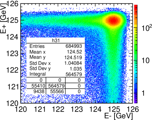
Figure 1: Distribution of the positron and electron beam energies at generator level for $\mathrm{e}^{+}\mathrm{e}^{-}\rightarrow\mu^{+}\mu^{-}(\gamma)$ events. The simulation includes the effects of beam energy spread and beamstrahlung.

Also shown in Figures 2,3,4,5 are the 1-d distributions at generator level of $E_{\mathrm{b}}^{+}$, $E_{\mathrm{b}}^{-}$, the center-of-mass energy, $\sqrt{s}$, and the distribution of ($E_{\mathrm{b}}^{-}-E_{\mathrm{b}}^{+}$)/2 for the same $\mathrm{e}^{+}\mathrm{e}^{-}\rightarrow\mu^{+}\mu^{-}(\gamma)$ events. The distributions have superimposed empirical fit models. Fit models are detailed in B.

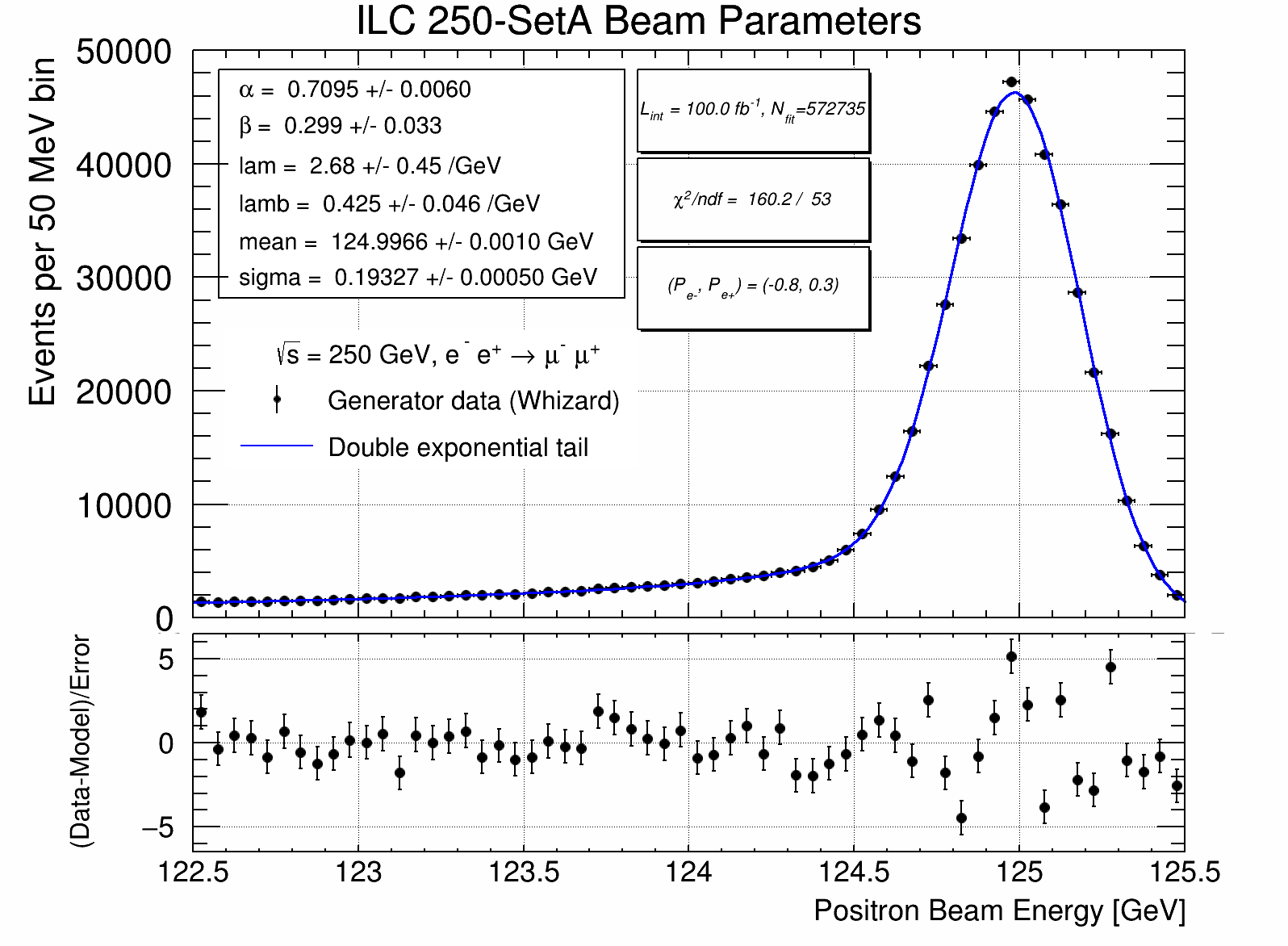
Figure 2: Distribution of the positron beam energy at generator level for $\mathrm{e}^{+}\mathrm{e}^{-}\rightarrow\mu^{+}\mu^{-}(\gamma)$ events with super-imposed 6-parameter fit. The simulation includes the effects of beam energy spread and beamstrahlung. Fit model details are discussed in B.

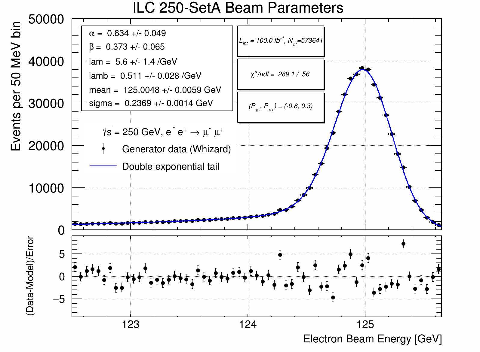
Figure 3: Distribution of the electron beam energy at generator level for $\mathrm{e}^{+}\mathrm{e}^{-}\rightarrow\mu^{+}\mu^{-}(\gamma)$ events with super-imposed 6-parameter fit. The simulation includes the effects of beam energy spread and beamstrahlung.

We see that the fitted Gaussian width parameters are roughly consistent with the expectations of 0.152% (positron) and 0.190% (electron). These beam energy fits don’t fit particularly well. Besides the possibility that the empirical model is inadequate, it is thought that there are at least two main underlying limitations in the degree of sophistication of the beam spectrum simulations that likely play a role in the poor fits. Firstly, the input beam energy distributions are truncated at about $\pm 3\sigma$. Secondly, the input beam energy distributions were sampled from a limited set of 80,000 particles per beam, so some of these particles have been used more than once. We have mitigated the effect of the former for now by limiting the maximum energy considered in these and other fits.

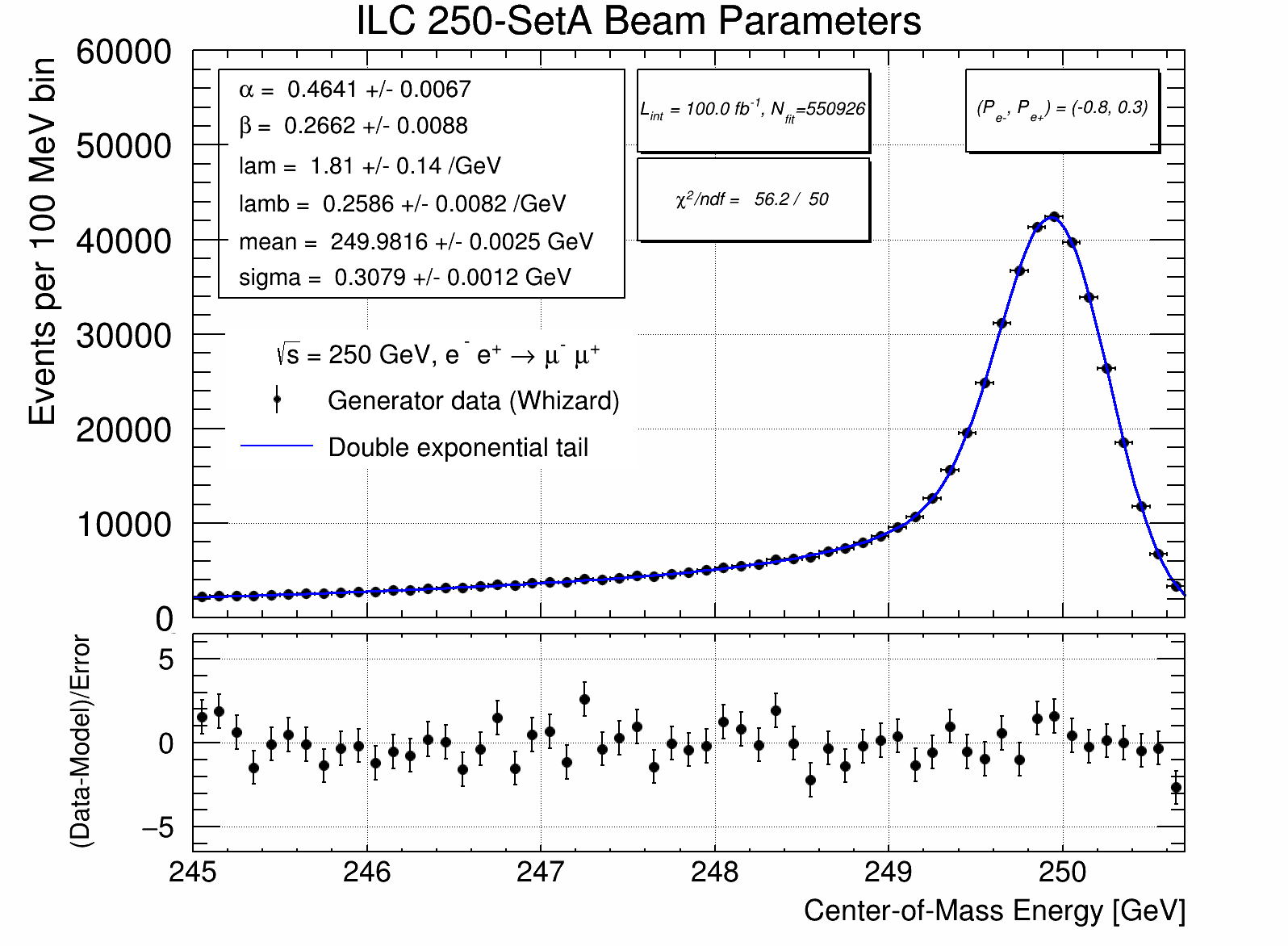
Figure 4: Generator level $\sqrt{s}$ distribution for $\mathrm{e}^{+}\mathrm{e}^{-}\rightarrow\mu^{+}\mu^{-}(\gamma)$ events with super-imposed 6-parameter fit.

By contrast the fit to the center-of-mass energy distribution (Figure 4) is very acceptable. It illustrates a fitted center-of-mass energy spread of 0.308 GeV namely, 0.123%, consistent with the expectation of 0.122%. Figure 5 shows that the modeled beam energy difference distribution is reasonably consistent with being symmetric. The overall width of the fitted central peak is about 22% larger than expected from simple Gaussian energy spread. This could be a consequence of the poor fit model, or maybe more likely a reflection that some of the 1-d peak in energy difference comes from the body of Figure 1 when both beams radiate beamstrahlung photons of similar energies. This distribution also makes clear that the electron and positron beam energies often differ by much more than an amount characteristic of simply the beam energy spread, leading to a mostly longitudinal boost to the actual collision in addition to the small horizontal transverse boost associated with the crossing angle. A key issue will be getting an experimental handle on these energy differences and it is expected that collision-based measurements of $\mathrm{e}^{+}\mathrm{e}^{-}\rightarrow\mu^{+}\mu^{-}(\gamma)$ events will also assist in the luminosity spectrum measurement.

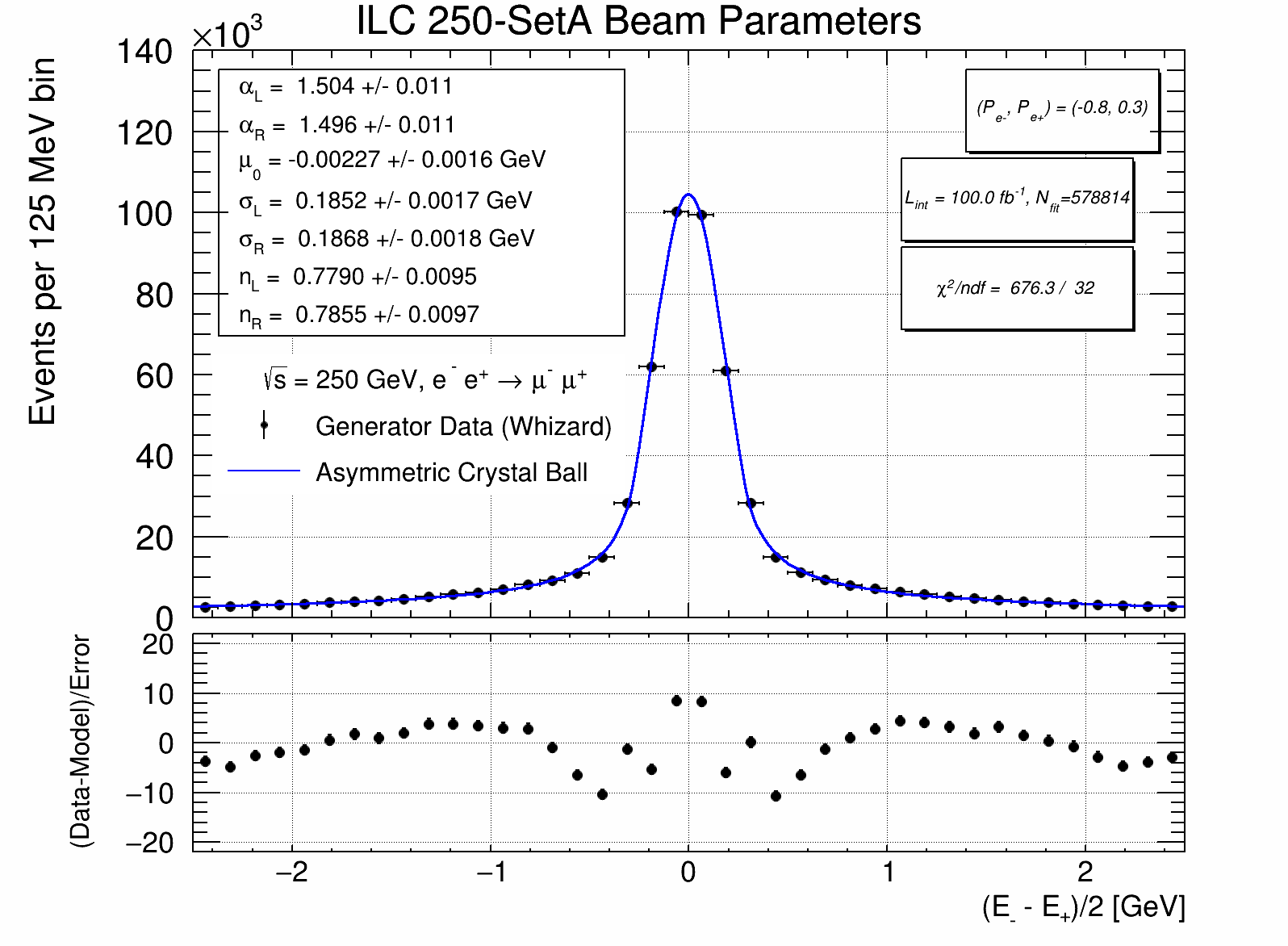
Figure 5: Generator level $\overline{\Delta E_{\mathrm{b}}}$ distribution for $\mathrm{e}^{+}\mathrm{e}^{-}\rightarrow\mu^{+}\mu^{-}(\gamma)$ events. We also super-imposed a two-sided Crystal Ball fit for illustration. We have used the general fit parametrization that allows for non-equal parameters on the left and right of the location parameter, $\mu_{0}$. Clearly in this case the observations are consistent with being symmetric. Note that for our current introductory purposes we are not concerned with parametrizing this distribution accurately.

3 Reconstructing $\sqrt{s}$ with muons

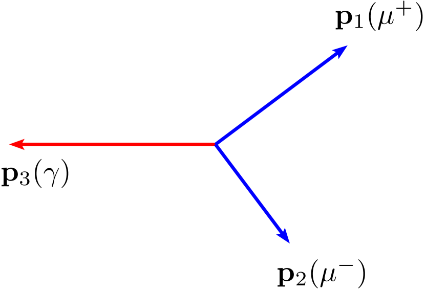
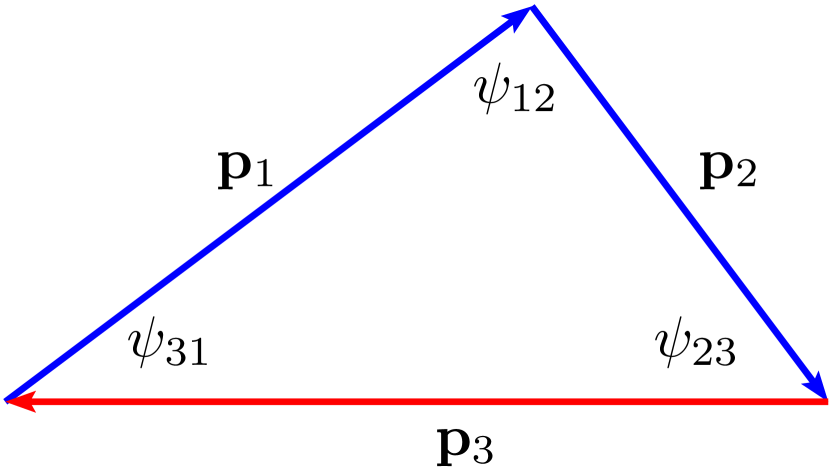
Figure 6: 3-body $\mu^{+}\mu^{-}\gamma$ final state with corresponding triangle construction obtained from 3-momentum conservation and the defined interior angles, $\psi_{12}$, $\psi_{23}$, $\psi_{31}$.

Before getting into details, we will present the basic underlying principles of the two methods. They were both initially developed very simplistically with the underlying assumption that the lab. system is the center-of-momentum system. Three-body kinematics are in fact rather special. When one has a final state consisting of three particles as in

$$\mathrm{e}^{+}\mathrm{e}^{-}\to{\mu_{1}}\!^{+}{\mu_{2}}\!^{-}\gamma\,_{3}\;\text{,}$$ (1)

under the assumption of 3-momentum conservation, and being in the center-of-momentum system, one can write the 3-momentum conservation equation, namely,

$$\mathrm{\mathbf{p}_{1}}+\mathrm{\mathbf{p}_{2}}+\mathrm{\mathbf{p}_{3}}=\mathrm{\mathbf{0}}\;\text{.}$$ (2)

One way of looking at this is to view this as a triangle as illustrated in Figure 6 with side lengths given by the magnitudes of each 3-momentum, $p_{1}$, $p_{2}$, $p_{3}$, and interior angles of the triangle, denoted, $\psi_{12}$, $\psi_{23}$, and $\psi_{31}$, where these necessarily satisfy, $\psi_{12}+\psi_{23}+\psi_{31}=\pi$. Each interior angle is the supplementary angle to the opening angle between each particle pair. The three opening angles can be calculated simply from the 3-vector scalar product, so we have

$$\psi_{12}\equiv\pi-\arccos\left(\frac{\mathrm{\mathbf{p}_{1}}\cdot\mathrm{\mathbf{p}_{2}}}{p_{1}\;p_{2}}\right),\psi_{23}\equiv\pi-\arccos\left(\frac{\mathrm{\mathbf{p}_{2}}\cdot\mathrm{\mathbf{p}_{3}}}{p_{2}\;p_{3}}\right),\psi_{31}\equiv\pi-\arccos\left(\frac{\mathrm{\mathbf{p}_{3}}\cdot\mathrm{\mathbf{p}_{1}}}{p_{3}\;p_{1}}\right)\;\text{.}$$ (3)

Given that we now have a triangle, we can apply a relationship between the sides and angles of the triangle, namely the triangle sine rule, resulting in,

$$\frac{p_{1}}{\sin{\psi_{23}}}=\frac{p_{2}}{\sin{\psi_{31}}}=\frac{p_{3}}{\sin{\psi_{12}}}\;\text{.}$$ (4)

We also define the center-of-mass scaled photon energy, $x_{\gamma}$. For this 3-body case this will satisfy

$$x_{\gamma}\equiv\frac{2E_{3}^{(*)}}{\sqrt{s}}=1-\frac{M_{12}^{2}}{s}\;\text{,}$$ (5)

where $M_{12}$ is the dimuon mass, $E_{3}$ is the photon energy, and we note with the ^(∗) notation that the photon energy needs to be evaluated in the center-of-momentum frame in general (as is the case here). Now using the energy conservation equation

$$E_{1}+E_{2}+E_{3}=\sqrt{s}\;\text{,}$$ (6)

or rather the version of this where we neglect the muon mass (the photon mass is of course zero),

$$p_{1}+p_{2}+p_{3}=\sqrt{s}\;\text{,}$$ (7)

with the triangle sine rule expressions we can now write each momentum magnitude in terms of $\sqrt{s}$ and functions of the measured interior angles by eliminating the other momenta,

$$\frac{p_{1}}{\sqrt{s}}=\frac{\sin{\psi_{23}}}{\sin{\psi_{12}}+\sin{\psi_{23}}+\sin{\psi_{31}}}\;\text{,}$$ (8)

$$\frac{p_{2}}{\sqrt{s}}=\frac{\sin{\psi_{31}}}{\sin{\psi_{12}}+\sin{\psi_{23}}+\sin{\psi_{31}}}\>\text{,}$$ (9)

$$\frac{p_{3}}{\sqrt{s}}=\frac{\sin{\psi_{12}}}{\sin{\psi_{12}}+\sin{\psi_{23}}+\sin{\psi_{31}}}\;\text{.}$$ (10)

With these three expressions we have at hand a very useful tool. With knowledge of $\sqrt{s}$ one can apply each expression to the prediction of the muon momentum scale and the photon energy scale relying only on the precise angular measurements.

Now turning to the direct utility for this paper. The dimuon invariant mass squared is

$$M_{12}^{2}=2(m^{2}+E_{1}E_{2}-p_{1}p_{2}\cos{\theta_{12}})\;\text{,}$$ (11)

where $\theta_{12}$ is the dimuon opening angle (ie. $\pi-\psi_{12}$). Again neglecting the muon mass, we get

$$M_{12}^{2}\approx 2p_{1}p_{2}(1-\cos{\theta_{12}})=2p_{1}p_{2}(1+\cos{\psi_{12}})\;\text{,}$$ (12)

and we can finally write

$$\frac{M_{12}^{2}}{s}=\frac{2p_{1}p_{2}(1+\cos{\psi_{12}})}{s}=\frac{2\sin{\psi_{23}}\sin{\psi_{31}}(1+\cos{\psi_{12}})}{(\sin{\psi_{12}}+\sin{\psi_{23}}+\sin{\psi_{31}})^{2}}\;\text{,}$$ (13)

There is scope to retain the fermion masses that were neglected in Equations 7 and 12. Such added complication does not seem warranted given that the correctable bias on $\sqrt{s}$ associated with this approximation for muons is only +2.9 ppm for $\mathrm{Z}\gamma$ with $M_{12}=m_{\mathrm{Z}}$ events at $\sqrt{s}=250$ GeV. Unsurprisingly, the bias for electrons is negligible (+70 ppb). It is more relevant for tau leptons, where the bias associated with omitting the mass is +0.08% (assuming perfect measurement of the tau lepton direction), and hadronic Z decays.

3.1 Angles method, $\sqrt{s}_{\psi}$

The angles method uses angular estimates of the square of the ratio of the di-fermion mass to the center of mass energy, such as Equation 13, in radiative return to the Z events, $\mathrm{e}^{+}\mathrm{e}^{-}\to\mathrm{Z}\gamma$, where the di-fermion mass is close to the Z mass. Given that $m_{\mathrm{Z}}$ is well known, one can rewrite this equation to construct an estimator for the center-of-mass energy, namely

$$\sqrt{s}_{\psi}=m_{\mathrm{Z}}\>\frac{\sin{\psi_{12}}+\sin{\psi_{23}}+\sin{\psi_{31}}}{\sqrt{2\sin{\psi_{23}}\>\sin{\psi_{31}}\>(1+\cos{\psi_{12}})}}\;\text{,}$$ (14)

where the fermion masses have been neglected, and one reconstructs the distribution of $\sqrt{s}_{\psi}$ under the assumption that the di-muon mass is actually $m_{\mathrm{Z}}$. A second-order polynomial parametrization for the statistical precision of this method vs $\sqrt{s}$ was reported in [17] for unpolarized beams for center-of-mass energies ranging from 250 to 1000 GeV. At $\sqrt{s}=250$ GeV, the statistical precision was found to be 28 MeV for 100 $\mathrm{fb}^{-1}$ corresponding to a relative statistical precision of 25 ppm for 2.0 $\mathrm{ab}^{-1}$ (unpolarized).

A similar expression for $x_{\gamma}$ can be formed using these angles. Other authors have used different conventions and notations for the angular measurements involved. We prefer this form for several reasons. Firstly, it retains a symmetry amongst the three particle pairs. Secondly, one of the interior angles is not explicitly eliminated using the $\psi_{12}+\psi_{23}+\psi_{31}=\pi$ constraint, and so one can use this as a test of the planarity assumption. Lastly, much of the literature has focused on using 3-body events in which the (ISR) photon is not in fact detected, and is assumed to be collinear with one of the beams. In this case with the beam $z$-axis defining the overall polar angle, it is then easy to confuse the polar angles of the muons with the angular separation of the muons from the photon.

The main perceived advantage of this method is that only precision angular measurements are required. There are four major limitations to this method.

1. It requires $\mathrm{Z}\gamma$ events. So it does not make use of full energy $\mathrm{e}^{+}\mathrm{e}^{-}\to\mu^{+}\mu^{-}$ events and will not be useful at $\sqrt{s}\approx m_{\mathrm{Z}}$.

2. It relies on knowledge of $m_{\mathrm{Z}}$. Currently this is 23 ppm. This will not be a limiting factor for anticipated measurements of $m_{\mathrm{t}}$ and $m_{\mathrm{H}}$, but current knowledge is a limiting factor for much improved measurements of $m_{\mathrm{W}}$ and especially $m_{\mathrm{Z}}$. On the other hand if $m_{\mathrm{Z}}$ were to be markedly improved for example by dedicated running at the Z-pole as envisaged for both FCC-ee [4] and ILC [9], this would be less of a factor for the utility of this method.

3. The intrinsic precision per $\mathrm{Z}\gamma$ event is reduced by the sizable contribution to the event-by-event estimates from the intrinsic width of the Z. The effective resolution per event on the center-of-mass energy from this source is $\Gamma_{\mathrm{Z}}/(\sqrt{2}m_{\mathrm{Z}})$ which equates to 1.9%.

4. At high center-of-mass energies, the large boost associated with $\mathrm{Z}\gamma$ events means that it is more and more difficult for each decay muon to be retained within the detector acceptance. Even at just $\sqrt{s}=500$ GeV both muons will have polar angles within $21^{\circ}$ of the beam axis.

3.2 Momentum method, $\sqrt{s}_{p}$

The overarching idea here is to just use the muon momenta, even if a photon is detected. For the simplifying assumption that the lab. system is the center-of-momentum system, independent of whether the $\mathrm{e}^{+}\mathrm{e}^{-}\rightarrow\mu^{+}\mu^{-}(\gamma)$ events are close to full energy $\mathrm{e}^{+}\mathrm{e}^{-}\to\mu^{+}\mu^{-}$ like events with no obvious evidence for photon radiation, or $\mathrm{e}^{+}\mathrm{e}^{-}\to\mu^{+}\mu^{-}\gamma$, one can construct an estimator of the center-of-mass energy under the assumption that the third particle system (the single photon in the previous discussion) is massless, by simply noting that Equation 2 can be re-expressed as

$$\mathrm{\mathbf{p}_{3}}=-(\mathrm{\mathbf{p}_{1}}+\mathrm{\mathbf{p}_{2}})\;\text{,}$$ (15)

and so the energy conservation equation (6), can be re-written simply as

$$E_{1}+E_{2}+|\mathrm{\mathbf{p}_{1}}+\mathrm{\mathbf{p}_{2}}|=\sqrt{s}\;\text{,}$$ (16)

retaining the fermion masses. Given that we are dealing with muons this results in the following estimator, that we denote, $\sqrt{s}_{p}$, where the equation has been rewritten to make the momentum dependence completely explicit for

$$\sqrt{s}_{p}=\sqrt{p_{1}^{2}+m_{\mu}^{2}}+\sqrt{p_{2}^{2}+m_{\mu}^{2}}+|\mathrm{\mathbf{p}_{1}}+\mathrm{\mathbf{p}_{2}}|\;\text{.}$$ (17)

The main advantage of this technique over the angles method is much better intrinsic precision per event presuming an ILC-like tracker. It does rely on knowing the tracker momentum scale with high precision. It also benefits from higher numbers of available events as it does not require $\mathrm{Z}\gamma$ events. One area of concern is that for events that are essentially 2-body events, namely, $\mathrm{e}^{+}\mathrm{e}^{-}\to\mu^{+}\mu^{-}$, the reconstruction method will always add in a third particle, a supposed photon, to balance the observed non-zero dimuon momentum that may arise simply from detector resolution. As we will see the statistical precision of this method for muons is an order of magnitude better than the angles method.

3.3 Mass method, $\sqrt{s}_{m}$

Given that we really do not want to necessarily assume the Z mass, but we have available the directly measured dimuon mass, with mass resolution much better than $\Gamma_{\mathrm{Z}}$, we can also rewrite Equation 13 simply as

$$\sqrt{s}_{m}=M_{12}\>\frac{\sin{\psi_{12}}+\sin{\psi_{23}}+\sin{\psi_{31}}}{\sqrt{2\sin{\psi_{23}}\>\sin{\psi_{31}}\>(1+\cos{\psi_{12}})}}\;\text{,}$$ (18)

where we measure the dimuon mass directly, including the mass terms, and use the angular measurements to infer the scaling to the center-of-mass energy for the radiated photon. This is hot off the press and it remains to be seen how complementary this approach is to $\sqrt{s}_{p}$. It looks less overtly a pure momentum-based measurement and appears to have exchanged a momentum-scale problem for a mass-scale problem, but we suspect this is naive given that the angles do also enter into Equation 17.

Some aspects of these methods are compared in Figure 7 based on generator level information in terms of the reconstructed $x_{\gamma}$ distributions either from muon angles or from knowledge of the mass of the dimuon and the actual center-of-mass energy. One expects a Breit-Wigner like peak centered at a photon energy of 108.4 GeV ($x_{\gamma}=0.8670$) for $\sqrt{s}=250$ GeV.

For the angles based method it is assumed that the photon is collinear with the beam particle that best accommodates momentum balance and is undetected. The simulation includes crossing angle effects so in principle these should be corrected for before measuring/calculating angles. A backward horizontal boost from the lab of $\beta=\sin(\alpha/2)$ is used in the green curve so that the newly calculated angles are in the nominal center-of-momentum frame. The black histogram neglects this correction. The blue and red histograms use the true dimuon mass directly, and the red histogram supplements this mass with any contributions from FSR photons as defined by the generator. The blue and red histograms also use the true center-of-mass energy. The width of the red histogram simply reflects the underlying Z width. Clearly there is some room for improvement by including FSR photons in the Z decay system. It is also apparent that the center-of-mass estimator with the angles-based method (green) will perform significantly worse than that implied by the intrinsic width of the Z alone unless more can be done to recuperate or correctly analyze the events that do not conform well to the assumptions.

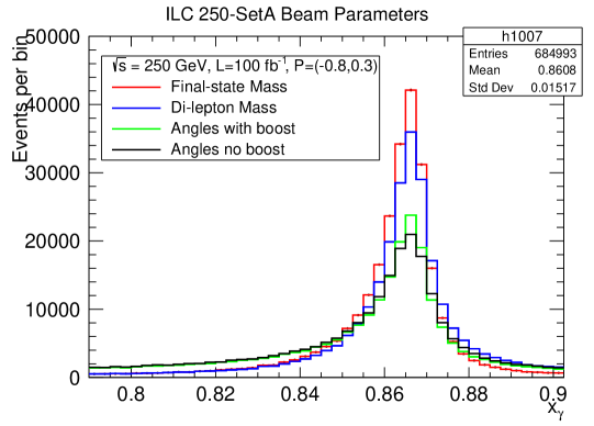
Figure 7: Comparison of different methods at generator level to reconstruct the peak in the center-of-mass scaled photon energy distribution of the assumed single photon in $\mathrm{Z}\gamma$ like dimuon events for $\sqrt{s}=250$ GeV. $x_{\gamma}$ is equivalent to $1-M_{12}^{2}/s$. The black and green histograms use angular reconstruction. The blue histogram uses the dimuon mass, and for the red histogram the mass estimate additionally includes contributions from FSR photons.

4 Realistic Kinematics for $\sqrt{s}_{p}$ Estimate

The main idea is again to use the kinematics of $\mathrm{e}^{+}\mathrm{e}^{-}\rightarrow\mu^{+}\mu^{-}(\gamma)$ events and measurements of the final-state particles to measure the distribution of the center-of-mass energy of collisions. The overall center-of-mass energy scale is provided by the tracker measurements of the muon momenta. In the real world, we need to add more realism to the picture of what happens in the collisions. Each line of the following adds more realism, but is still in some aspects idealized:

1. Nominal. Each beam is a delta function centered at a particular beam energy, and the lab. frame is the center-of-momentum frame.

2. Crossing Angle ($\alpha$). In practice beams will have a small net horizontal momentum that leads to the detector (ie lab.) reference frame never being the center-of-momentum frame.

3. Beam energy spread (BES). Each beam naturally has an energy spread that reflects the production, damping, transport, bunch compression, acceleration, and focusing associated with preparation of the beam for delivery to the interaction point. A simplifying assumption is to use a Gaussian energy distribution. More realistic models for ILC should include likely energy-$z$ correlations that can be modeled with an end-to-end accelerator simulation, and may be constrained with beam diagnostics. Additionally each beamline is independent so there is no expectation that the two beam energies are identical.

4. BES + Beamstrahlung (BS). The collective interaction of the two beams leads to radiation of photons referred to as beamstrahlung photons from the beams, resulting in a beamstrahlung-reduced center-of-mass energy.

5. BES + BS + Initial-state-radiation (ISR). All $\mathrm{e}^{+}\mathrm{e}^{-}$ physics processes may have ISR, where the invariant mass of the annihilating $\mathrm{e}^{+}\mathrm{e}^{-}$ and the resulting particle system (excluding the ISR photon(s)) is reduced compared with case 3 due to the emitted ISR photon(s).

We will be primarily concerned with evaluating the beamstrahlung-reduced center-of-mass energy. This is after beam energy spread and beamstrahlung radiation, but before emission of any ISR photons. We will allow for differences in the energy of each beam and for a beam crossing angle, $\alpha$, defined as the horizontal plane angle between the two beam lines. For ILC $\alpha$ is 14 mrad.

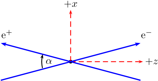
Figure 8: The $z$-axis is defined as the axis that bisects the outgoing electron beam-line axis and the negative of the incoming positron beam-line axis. The $x$-axis is the horizontal axis in the direction of the net horizontal momentum of the initial state.

There are a number of formulations of the kinematic problem that differ in what are the assumptions, the measurements, and the setup. We focus on the system of 4-vectors comprising the $\mathrm{e}^{+}\mathrm{e}^{-}$ after beamstrahlung emission as measured in the detector reference frame illustrated and defined in Figure 8. Note that given the crossing angle, this reference frame is not the center-of-momentum frame.

Let’s define the two beam energies (after beamstrahlung) as $E_{\mathrm{b}}^{-}$ and $E_{\mathrm{b}}^{+}$ for the electron and positron beam respectively, and define for simplicity, $s_{\alpha}=\sin(\alpha/2)$, $c_{\alpha}=\cos(\alpha/2)$ and $t_{\alpha}=\tan(\alpha/2)$. This leads to an initial-state energy-momentum 4-vector $(E,\>p_{x},p_{y},p_{z})$ consisting of

$$E =E_{\mathrm{b}}^{-}+E_{\mathrm{b}}^{+}\;\text{,}$$ (19)

$$p_{x} =(E_{\mathrm{b}}^{-}+E_{\mathrm{b}}^{+})\>s_{\alpha}\;\text{,}$$ (20)

$$p_{y} =0\;\text{,}$$ (21)

$$p_{z} =(E_{\mathrm{b}}^{-}-E_{\mathrm{b}}^{+})\>c_{\alpha}\;\text{,}$$ (22)

where we have neglected the electron mass.

The corresponding center-of-mass energy (the invariant mass of the initial-state 4-vector) is

$$\sqrt{s}=2\sqrt{E_{\mathrm{b}}^{-}E_{\mathrm{b}}^{+}}\>c_{\alpha}\;\text{.}$$ (23)

Hence if $\alpha$ is known, evaluation of the center-of-mass energy of this collision amounts to measuring the two beam energies. It is convenient to introduce the average of the two beam energies, $E_{\mathrm{ave}}$, and half of the beam energy difference, $\overline{\Delta E_{\mathrm{b}}}$,

$$E_{\mathrm{ave}}\equiv\frac{E_{\mathrm{b}}^{-}+E_{\mathrm{b}}^{+}}{2}\;\text{,}$$ (24)

$$\overline{\Delta E_{\mathrm{b}}}\equiv\frac{E_{\mathrm{b}}^{-}-E_{\mathrm{b}}^{+}}{2}\;\text{.}$$ (25)

With this notation

$$\sqrt{s}=2\sqrt{E_{\mathrm{ave}}^{2}-(\overline{\Delta E_{\mathrm{b}}})^{2}}\>c_{\alpha}\;\text{,}$$ (26)

$$p_{z}=2\;\overline{\Delta E_{\mathrm{b}}}\>c_{\alpha}\;\text{,}$$ (27)

and we can define the initial-state $\mathrm{e}^{+}\mathrm{e}^{-}$ system 4-vector components as

$$(E_{\mathrm{ini}},\mathrm{\mathbf{p}}_{\mathrm{ini}})\equiv 2(E_{\mathrm{ave}},\;E_{\mathrm{ave}}\;s_{\alpha},\;0,\;\overline{\Delta E_{\mathrm{b}}}\;c_{\alpha})\;\text{.}$$ (28)

Now let’s look at the final state of the $\mathrm{e}^{+}\mathrm{e}^{-}\rightarrow\mu^{+}\mu^{-}(\gamma)$ process. We will denote the $\mu^{+}$ as particle 1, the $\mu^{-}$ as particle 2, and the rest-of-the event as system 3. In the simple case of $\mathrm{e}^{+}\mathrm{e}^{-}\to\mu^{+}\mu^{-}$, with only two produced particles, the rest-of-the event is the null vector. In the case of one single photon, the rest-of-the-event is this one photon. In the case of multiple photons, the rest-of-the-event is this system of multiple photons, that may or may not have significant mass. The photons are often ISR photons that tend to be at forward angles and can be undetectable.

We can write this final-state system 4-vector as

$$(E_{1}+E_{2}+E_{3},\>\mathrm{\mathbf{p}}_{1}+\mathrm{\mathbf{p}}_{2}+\mathrm{\mathbf{p}}_{3})\;\text{.}$$ (29)

In general the rest-of-the-event system will not be fully detected and needs to be inferred using energy-momentum conservation or additional assumptions on especially its mass. In full generality let’s keep non-zero mass for the rest-of-the event mass, $M_{3}$. Then proceeding to apply energy-momentum conservation by equating the above to the initial-state 4-vector we obtain

$$E_{1}+E_{2}+\sqrt{p_{3}^{2}+M_{3}^{2}}=2\;E_{\mathrm{ave}}\;\text{,}$$ (30)

$$\mathrm{\mathbf{p}}_{1}+\mathrm{\mathbf{p}}_{2}+\mathrm{\mathbf{p}}_{3}=\mathrm{\mathbf{p}}_{\mathrm{ini}}=2(\;E_{\mathrm{ave}}\>s_{\alpha},\;0,\;\overline{\Delta E_{\mathrm{b}}}\>c_{\alpha})\;\text{.}$$ (31)

This represents the four equations of energy-momentum conservation and six unknowns, namely the three components of the rest-of-the-event 3-momentum, $\mathrm{\mathbf{p}}_{3}$, the two beam energy related quantities, $E_{\mathrm{ave}}$, $\overline{\Delta E_{\mathrm{b}}}$ and the rest-of-the-event mass $M_{3}$. Further progress needs additional assumptions. A general way to approach the problem is to solve for $E_{\mathrm{ave}}$ for various assumptions on $\overline{\Delta E_{\mathrm{b}}}$ and $M_{3}$. Specifically we will then focus on using the simplifying assumptions that $\overline{\Delta E_{\mathrm{b}}}=0$ and $M_{3}=0$. The $\overline{\Delta E_{\mathrm{b}}}$ assumption is a poor one event-by-event for the $p_{z}$ conservation component as can be deduced from Figure 5. In the following, we solve the general problem ($\overline{\Delta E_{\mathrm{b}}}$ and $M_{3}$ non-zero) and make no assumption on the direction of the rest-of-the event particles, apart from their total invariant mass.

We can write

$$\mathrm{\mathbf{p}}_{3}=\mathrm{\mathbf{p}}_{\mathrm{ini}}-(\mathrm{\mathbf{p}}_{1}+\mathrm{\mathbf{p}}_{2})\;\text{,}$$ (32)

and using

$$|\mathrm{\mathbf{a}}-\mathrm{\mathbf{b}}|=\sqrt{a^{2}+b^{2}-2\;\mathrm{\mathbf{a}}\cdot\mathrm{\mathbf{b}}}\;\text{,}$$ (33)

find

$$|\mathrm{\mathbf{p}}_{3}|=\sqrt{p_{\mathrm{ini}}^{2}+(p_{12})^{2}-4(p_{12}^{x})E_{\mathrm{ave}}\>s_{\alpha}-4(p_{12}^{z})\overline{\Delta E_{\mathrm{b}}}\>c_{\alpha}}\;\text{.}$$ (34)

Now using equation 30 we can write,

$$p_{3}^{2}=(2E_{\mathrm{ave}}-E_{1}-E_{2})^{2}-M_{3}^{2}\;\text{,}$$ (35)

and by equating this to the square of equation 34, we eliminate $\mathrm{\mathbf{p}}_{3}$,

$$(2E_{\mathrm{ave}}-E_{1}-E_{2})^{2}-M_{3}^{2}=p_{\mathrm{ini}}^{2}+(p_{12})^{2}-4(p_{12}^{x})E_{\mathrm{ave}}\>s_{\alpha}-4(p_{12}^{z})\overline{\Delta E_{\mathrm{b}}}\>c_{\alpha}\;\text{.}$$ (36)

Now inserting the components of $\mathrm{\mathbf{p}}_{\mathrm{ini}}$, we find,

$$(2E_{\mathrm{ave}}-E_{12})^{2}-M_{3}^{2}=4E_{\mathrm{ave}}^{2}s_{\alpha}^{2}+4\overline{\Delta E_{\mathrm{b}}}^{2}c_{\alpha}^{2}\\ +(p_{12})^{2}-4(p_{12}^{x})E_{\mathrm{ave}}s_{\alpha}-4(p_{12}^{z})\overline{\Delta E_{\mathrm{b}}}c_{\alpha}\;\text{.}$$ (37)

This is a quadratic

$$AE_{\mathrm{ave}}^{2}+BE_{\mathrm{ave}}+C=0\;\text{,}$$ (38)

in $E_{\mathrm{ave}}$ with coefficients (after simplification) of

$$A =c_{\alpha}^{2}\;\text{,}$$ (39)

$$B =-E_{12}\;+\;p_{12}^{x}\>s_{\alpha}\;\text{,}$$ (40)

$$C =(M_{12}^{2}-M_{3}^{2})/4\;+\;p_{12}^{z}\overline{\Delta E_{\mathrm{b}}}\>c_{\alpha}\;-\;\overline{\Delta E_{\mathrm{b}}}^{2}\>c_{\alpha}^{2}\;\text{.}$$ (41)

Based on this, there are three particular cases of interest which can be solved for $E_{\mathrm{ave}}$ with in the first instance, $M_{3}=0$,

1. Zero crossing angle, $\alpha=0$, and zero beam energy difference.

2. Crossing angle and zero beam energy difference.

3. Crossing angle and non-zero beam energy difference.

The original studies led to the relationship

$$\sqrt{s}=E_{1}+E_{2}+|\mathrm{\mathbf{p}}_{12}|\;\text{,}$$ (42)

and this arises of course essentially trivially in the first case. Explicitly for this case, we have

$$A=1,B=-E_{12},C=(M_{12}^{2})/4\;\text{,}$$ (43)

with a resulting discriminant of

$$B^{2}-4AC=E_{12}^{2}-M_{12}^{2}=p_{12}^{2}\;\text{,}$$ (44)

and solutions of

$$E_{\mathrm{ave}}=\frac{E_{12}\pm|\mathrm{\mathbf{p}}_{12}|}{2}\;\text{,}$$ (45)

leading to

$$\sqrt{s}=2\;E_{\mathrm{ave}}=E_{12}\pm|\mathrm{\mathbf{p}}_{12}|\;\text{.}$$ (46)

Only the positive solution is physical given that the $E_{3}$ contribution to the center-of-mass energy needs to be non-negative.

For cases, 2 and 3, the discriminant is always positive. It also seems that it is always the positive solution that yields the correct physical solution for $E_{\mathrm{ave}}$. Given that the crossing angle is small, and the expected energy differences are relatively small, it is not unexpected that the more complete cases find solutions similar to the most approximate one (case 1). We have also re-derived the result of case 2 as a quadratic directly in terms of $\sqrt{s}$. This alternative formulation is described in A for completeness, and leads explicitly to the observation that the case 2 estimate, can be viewed simply as

$$\sqrt{s}_{p}=E_{12}^{*}+|\mathrm{\mathbf{p}}_{12}^{*}|\;\text{.}$$ (47)

Figure 9 shows the generator level distribution of $\sqrt{s}_{p}$ evaluated with case 2 together with the same double exponential tail fit previously used for the true $\sqrt{s}$ distribution. Figure 10 shows the distribution of $\sqrt{s}_{p}$ evaluated with case 3 where one assumes one knows the true value of $\overline{\Delta E_{\mathrm{b}}}$. It is noteworthy that the degradation of the peak width under the $\overline{\Delta E_{\mathrm{b}}}=0$ assumption is recuperated by using the correct value for $\overline{\Delta E_{\mathrm{b}}}$. Similarly, Figure 11 shows the distribution of $\sqrt{s}_{p}$ evaluated with the usual equal beam energies assumption, but in this case imposing the true value of $M_{3}$ rather than the assumed value of zero. In this case the peak width is very similar to case 2 (3% smaller) indicating that the $M_{3}=0$ assumption by itself does not degrade the peak width substantially. However, one can see that significantly more events, that were previously undermeasured, are now found in the peak region.

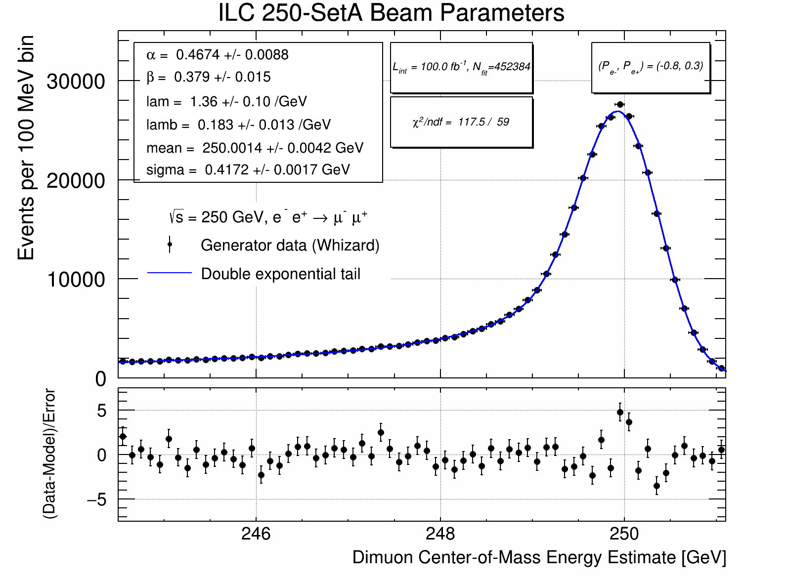
Figure 9: Generator level $\sqrt{s}_{p}$ distribution evaluated with generator-level muons for $\mathrm{e}^{+}\mathrm{e}^{-}\rightarrow\mu^{+}\mu^{-}(\gamma)$ events with super-imposed 6-parameter fit.

Figure 10: Generator level $\sqrt{s}_{p}$ distribution evaluated with generator-level muons for $\mathrm{e}^{+}\mathrm{e}^{-}\rightarrow\mu^{+}\mu^{-}(\gamma)$ events with super-imposed 6-parameter fit. In this case the true event-by-event value of the (halved) beam energy difference of Figure 5 is used, rather than assuming that it is zero.

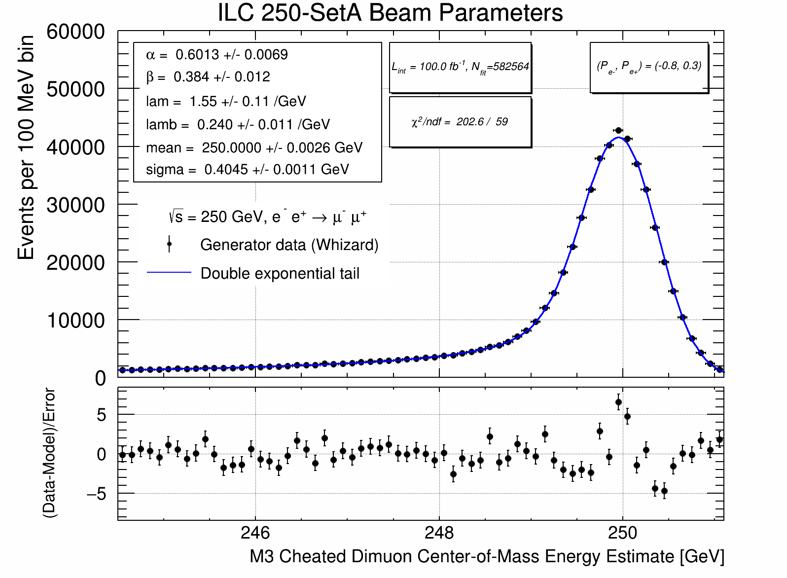
Figure 11: Generator level $\sqrt{s}_{p}$ distribution evaluated with generator-level muons for $\mathrm{e}^{+}\mathrm{e}^{-}\rightarrow\mu^{+}\mu^{-}(\gamma)$ events with super-imposed 6-parameter fit where the true event-by-event $M_{3}$ value is used.

Table 1 lists various kinematic quantities at generator-level for six illustrative events. As expected, when $M_{3}$ is small, the $\overline{\Delta E_{\mathrm{b}}}$ cheated $\sqrt{s}_{p}$ estimate is identical to the true $\sqrt{s}$ (Events 1,2,4,5,6). Additionally, when $\overline{\Delta E_{\mathrm{b}}}$ is also small, the $\sqrt{s}_{p}$ estimate agrees rather well with the true $\sqrt{s}$ for both radiative-return Z type events (Event 1) and full-energy events (Event 4). Events 2, 5, and 6 have large values of $|\overline{\Delta E_{\mathrm{b}}}|$ leading to large deviations in $\sqrt{s}_{p}$ from $\sqrt{s}$. In event 2, where there is no photon, the $\sqrt{s}_{p}$ estimator overestimates by about $2|\overline{\Delta E_{\mathrm{b}}}|$ over $M_{12}$ by adding a fictitious 10 GeV photon in the electron direction. While in events 5 and 6, the $\sqrt{s}_{p}$ estimator either largely overestimates or largely underestimates $\sqrt{s}$ depending on whether the inferred photonic system is in the same or opposite hemisphere to the direction of the initial state $\overline{\Delta E_{\mathrm{b}}}$ induced boost. The biases are obviously big for these two individual events, but the main effect is a tendency to broaden the estimated $\sqrt{s}$ since radiation of ISR photons should occur symmetrically for the electron and positron beams. Lastly, event 3 has a massive photonic system, and a substantial $|\overline{\Delta E_{\mathrm{b}}}|$ which is then problematic for both the $M_{3}=0$ and $\overline{\Delta E_{\mathrm{b}}}=0$ assumptions.

Event	1	2	3	4	5	6
$E_{\mathrm{b}}^{-}$	125.34	114.55	125.32	124.87	124.75	122.77
$E_{\mathrm{b}}^{+}$	124.82	124.64	121.08	124.49	116.24	110.12
$\overline{\Delta E_{\mathrm{b}}}$	$+0.26$	$-5.04$	$+2.12$	$+0.19$	$+4.26$	$+6.33$
$M_{12}$	92.55	238.97	94.62	249.30	82.34	92.26
$p_{12}$	108.41	10.22	104.74	1.73	101.66	105.43
$p_{12}^{x}$	$+18.82$	$+1.67$	$+1.25$	$+1.70$	$+0.92$	$+1.03$
$p_{12}^{y}$	$-14.54$	0.00	$+0.21$	$-0.01$	0.00	$-0.25$
$p_{12}^{z}$	$+105.77$	$-10.08$	$+104.73$	$+0.35$	$-101.65$	$+105.43$
$p_{3}$	107.62	0.00	100.49	0.06	110.17	92.78
$M_{3}$	0.00	0.00	31.27	0.00	0.55	0.00
$\sqrt{s}$	250.15	238.97	246.35	249.35	240.84	232.53
$E_{12}^{*}$ ($\beta_{x}$)	142.41	239.18	141.15	249.30	130.82	140.10
$p_{12}^{*}$ ($\beta_{x}$)	108.24	10.08	104.73	0.35	101.65	105.43
$\sqrt{s}_{p}$	250.65	249.26	245.88	249.65	232.47	245.53
$E_{12}^{*}$ ($\beta_{x},\beta_{z}$)	142.20	238.97	139.36	249.30	134.49	134.57
$p_{12}^{*}$ ($\beta_{x},\beta_{z}$)	107.96	0.00	102.32	0.06	106.34	97.96
$\sqrt{s}_{p}$ (true $\overline{\Delta E_{\mathrm{b}}}$)	250.15	238.97	241.60	249.35	240.84	232.53
$\sqrt{s}_{p}$ (true $M_{3}$)	250.65	249.26	250.45	249.65	232.47	245.53

Table 1: Generator-level kinematic quantities (GeV) for illustrative events. Energies and momenta are given in the lab. frame except for $E_{12}^{*}$ and $p_{12}^{*}=\sqrt{(E_{12}^{*})^{2}-M_{12}^{2}}$ which are the dimuon energy and momentum after boosting according to either the Case 2 $\sqrt{s}_{p}$ assumptions ($\beta_{x}$) or the correct Case 3 boost ($\beta_{x}$, $\beta_{z}$) as discussed in A.

5 Dimuon event selection and reconstruction

The event selection used is very simple given that it is not expected that backgrounds will be quantitatively important. Detector acceptance is the main limiting factor for overall efficiency and this is particularly true for reconstructing $\mathrm{e}^{+}\mathrm{e}^{-}\rightarrow\mu^{+}\mu^{-}(\gamma)$ events where the dimuon mass is very low. Quality of momentum reconstruction is very important for reconstructing $\sqrt{s}$ with this method and this is a strong function of polar angle. The generated $\mathrm{e}^{+}\mathrm{e}^{-}\rightarrow\mu^{+}\mu^{-}(\gamma)$ events are from two samples one using $P_{\mathrm{e^{-}}}=-1.0,P_{\mathrm{e^{+}}}=+1.0$ (LR) with a cross-section of 11.18 pb and one using $P_{\mathrm{e^{-}}}=+1.0,P_{\mathrm{e^{+}}}=-1.0$ (RL) with a cross-section of 8.80 pb. These are mixed together to form partially polarized (80%/30%) mixtures for the four helicity combinations (LR, RL, LL, RR) associated with the standard ILC running scenario with integrated luminosity fractions of (45%, 45%, 5%, 5%) respectively.

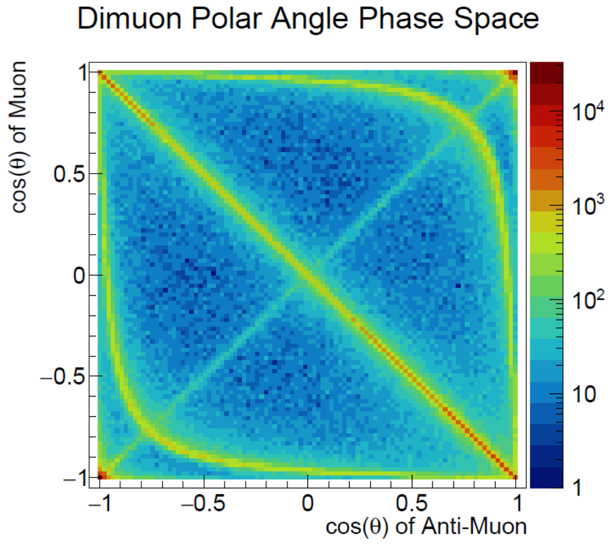
Figure 12: Generator level distribution of the cosines of the muon polar angles for $\sqrt{s}=250$ GeV for $\mathrm{e}^{+}\mathrm{e}^{-}\rightarrow\mu^{+}\mu^{-}(\gamma)$ with $P(\mathrm{e}^{-})=-0.8$ and $P(\mathrm{e}^{+})=+0.3$.

Figure 12 illustrates the distribution of the cosine of the muon polar angles at generator level for $\sqrt{s}=250$ GeV. The events include dimuons with $M_{\mu\mu}$ near “full-energy” of 250 GeV, the radiative-return to the Z events with $M_{\mu\mu}\approx m_{\mathrm{Z}}$ and radiative events with much lower $M_{\mu\mu}$ extending all the way to the threshold at $2m_{\mu}$. The full-energy events populate the collinear region of this figure where the two muons tend to be back-to-back in space (the descending diagonal). The radiative-return to the Z events populate the two relatively narrow hyperbola regions (the width is dictated partly by $\Gamma_{\mathrm{Z}}$). The lower-left/upper-right hyperbola regions correspond to emission of an approximately 108 GeV ISR photon by the electron/positron beam respectively. Additionally there are populated regions at the extreme lower-left and upper-right arising from radiative-return to very low mass where the dimuon system tends to be at very forward angle balancing an essentially beam energy ISR photon emitted preferentially close to the beam axis. Lastly the events on the ascending diagonal are (much rarer) events with rather low $M_{\mu\mu}$ where the beam energy photon is scattered at large polar angle, resulting in two muons of low mass but with dimuon energy close to the beam energy going in very similar directions.

The study uses the latest ILD full simulation and reconstruction samples based on the ILC accelerator model at $\sqrt{s}=250$ GeV for beam energy spread and beamstrahlung and the IDR-L detector model described in [22]. The event selection criteria applied are:

• Require exactly two reconstructed muon particle flow objects and require that they have opposite charge (84.1% pass).

• Require that the calculated uncertainty on $\sqrt{s}_{p}$ computed from the two muons be less than 0.8% of the nominal center-of-mass energy of 250 GeV (72.2% pass). This is based on propagating the track error matrices.

• Require that the two muons pass a common vertex fit with p-value exceeding 1% (70.4% pass). This reduces non-prompt backgrounds such as events where one of the muons is from a muonically decaying tau lepton. It also likely makes the $\sqrt{s}_{p}$ estimate more robust, and facilitates future studies of primary vertex position dependence of the luminosity spectrum.

Given above in parentheses are the fractions of LR mixture events surviving these sequential criteria. The reconstruction quality in terms of the calculated $\sqrt{s}_{p}$ uncertainty as a fraction of the nominal center-of-mass energy is used to define three dimuon event quality categories: gold, silver, and bronze for $<0.15$%, [0.15%, 0.30%], and [0.30%, 0.80%] respectively.

The overall efficiency including acceptance effects to pass all criteria is about 69.2% averaged over the helicity combinations. The (background) efficiency for selecting $\mathrm{e}^{+}\mathrm{e}^{-}\to\tau^{+}\tau^{-}(\gamma)$ events is small (about 0.15%). A detailed background study is beyond the scope of the current work.

Figure 13: Reconstruction level $\sqrt{s}_{p}$ distribution evaluated with muon particle flow objects for $\mathrm{e}^{+}\mathrm{e}^{-}\rightarrow\mu^{+}\mu^{-}(\gamma)$ events with super-imposed 6-parameter fit where the dimuon $\sqrt{s}_{p}$ resolution satisfies the gold quality criterion.

The reconstructed $\sqrt{s}_{p}$ distributions are shown in Figures 13, 14, and 15 for the gold, silver, and bronze categories, respectively. The empirical fit model (double exponential tail) works reasonably well; it manages to accommodate the combined effects from energy spread, beamstrahlung, detector resolution, ISR, and FSR. As expected the widths of the peaks degrade from gold to silver to bronze. A more refined analysis would try to exploit this per event resolution information at the event-to-event level, but for now we confine ourselves to estimates of the precision on the center-of-mass energy scale from these three separate categories. These are shown in Table 2 for the four different data-sets associated with the ILC standard run plan at $\sqrt{s}=250$ GeV as well as for unpolarized beams for comparison. Here we have fixed the shape parameters of the fits (based on the best fit) and only fit for the peak location parameter. We have done similar studies using the asymmetric Crystal Ball fit model and find essentially the same results for statistical precision, but appreciably different values of $\mu$ as may be expected. Both fit models are described in B. Overall the statistical uncertainty associated with the 2 $\mathrm{ab}^{-1}$ dataset is 1.9 ppm on the center-of-mass energy scale.

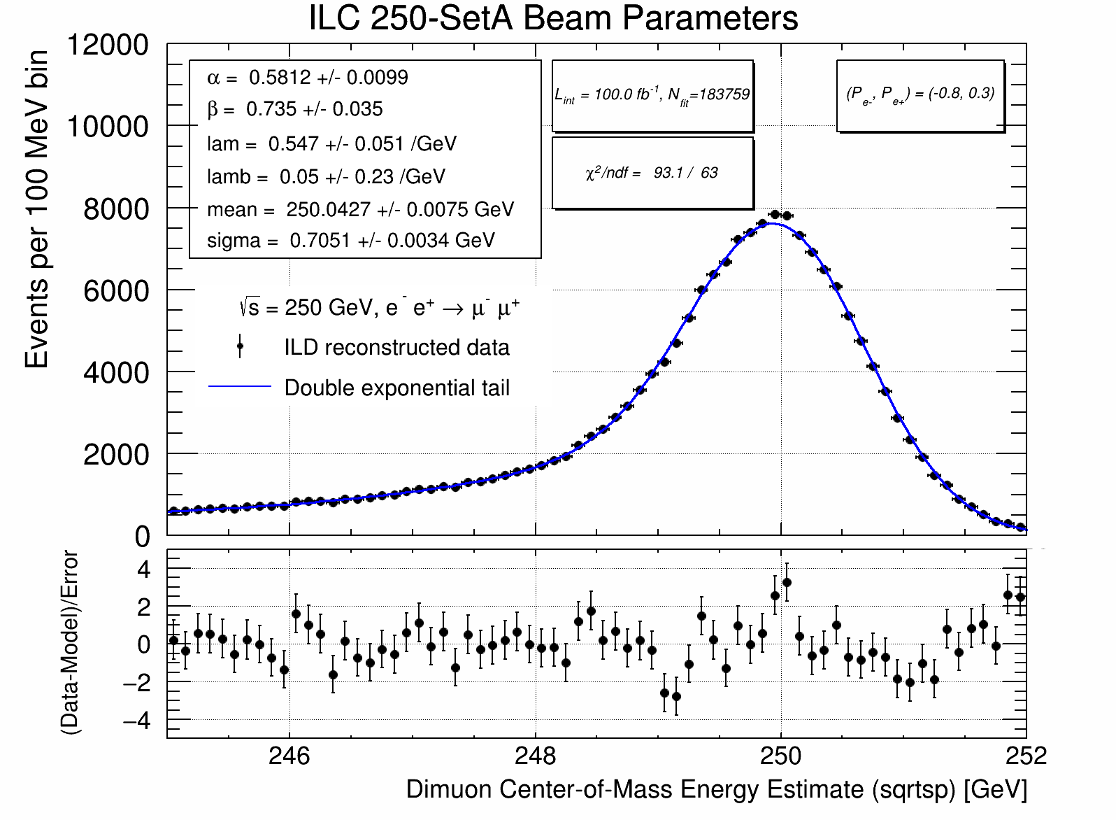
Figure 14: Reconstruction level $\sqrt{s}_{p}$ distribution evaluated with muon particle flow objects for $\mathrm{e}^{+}\mathrm{e}^{-}\rightarrow\mu^{+}\mu^{-}(\gamma)$ events with super-imposed 6-parameter fit where the dimuon $\sqrt{s}_{p}$ resolution satisfies the silver quality criterion.

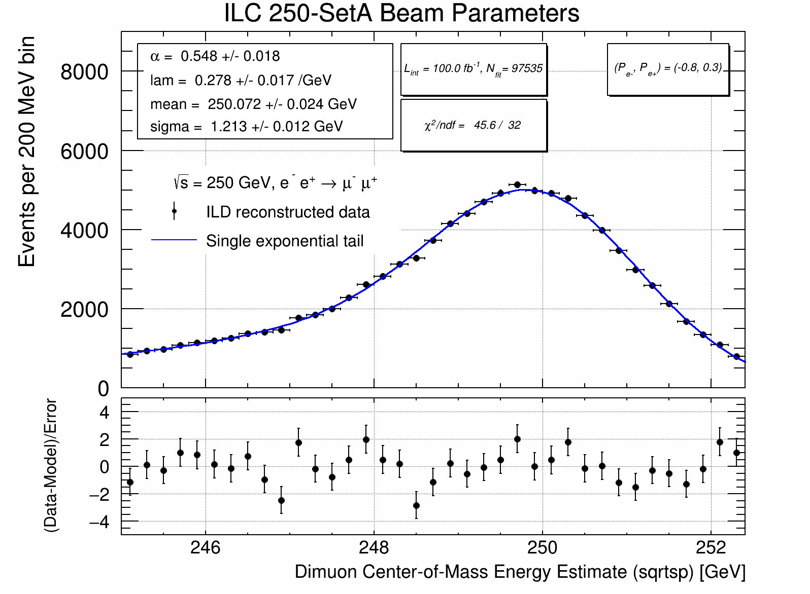
Figure 15: Reconstruction level $\sqrt{s}_{p}$ distribution evaluated with muon particle flow objects for $\mathrm{e}^{+}\mathrm{e}^{-}\rightarrow\mu^{+}\mu^{-}(\gamma)$ events with super-imposed 6-parameter fit where the dimuon $\sqrt{s}_{p}$ resolution satisfies the bronze quality criterion. In this case a single exponential tail component is sufficient.

$L_{\mathrm{int}}$ [ab-1]	Poln [%]	Efficiency [%]	Gold	Silver	Bronze	All categories
2.0	$0,0$	69.3	5.1	2.4	6.1	2.1
0.9	$-80,+30$	70.4	6.4	3.1	7.7	2.6
0.9	$+80,-30$	68.0	7.5	3.4	8.7	2.9
0.1	$-80,-30$	70.1	25	12	30	10
0.1	$+80,+30$	68.3	28	13	33	11
2.0	Combined	-	4.7	2.2	5.6	1.9

Table 2: Fractional statistical uncertainties in parts per million (ppm) on the mean parameter, $\mu$, of the Gaussian peak component of the measured $\sqrt{s}_{p}$ distribution for $\sqrt{s}=250$ GeV ILC running (4 data-sets with different beam polarizations) from fits to the gold, silver, and bronze categories of dimuons. These are 1-parameter fits where the model shape parameters are fixed to their best fit values. For gold and silver categories, the fit uses the double exponential tail function, while for bronze it uses the single exponential tail function. Fit ranges and binning are as indicated in Figures 13, 14, and 15. The all categories column shows the weighted statistical uncertainty assuming that all data-set columns are used in each weighted average. The last row shows the combination of the four 80%/30% polarization data-sets. Also shown for comparison in the first row is the result for unpolarized beams.

We justify focusing for now on this seemingly artificial single parameter fit because we expect the shape parameters to be much better measured using Bhabhas in the luminosity spectrum measurement, and they should also be constrained to some extent by accelerator diagnostics measurements. The main goal of the dimuon studies is to pin down the absolute center-of-mass energy scale that is of prime importance from the physics perspective. It is also expected that the shape sensitivity can be improved, (and the correlations on $\mu$ reduced), by widening the fit range.

Fits have also been performed where the peak mean and width are fitted with the other shape parameters fixed, leading to at most a 9% degradation in the precision of the scale parameter, $\mu$. It is expected that by applying $\sqrt{s}_{p}$ to Bhabha events and using in this case the tracker-based electron momentum measurement that a substantial increase in precision should also be feasible.

$L_{\mathrm{int}}$ [ab-1]	Poln [%]	Gold	Silver	Bronze
0.1	$-80,+30$	$249.9273\pm 0.0048$	$250.0422\pm 0.0023$	$250.0715\pm 0.0058$
0.1	$+80,-30$	$249.9335\pm 0.0056$	$250.0541\pm 0.0026$	$250.0972\pm 0.0066$

Table 3: Results of the 1-parameter fits to the reconstructed $\sqrt{s}_{p}$ distribution for the $\mu$ parameter in units of GeV for the three different categories for the two main helicity mixtures. This uses the same integrated luminosity as the figures (100 $\mathrm{fb}^{-1}$) rather than scaling these numbers to the ILC standard running scenario as done in Table 2.

We also show in Table 3 the fitted $\mu$ values for six of the fits. It is noteworthy that the fitted $\mu$ values depend markedly on dimuon reconstruction quality. We attribute some of this to the expectation that high-mass events with little missing momentum are liable to be over-measured as a result of momentum resolution. It is also the case that the relative fractions of radiative-return to the Z and high-energy events is a strong function of the $\sqrt{s}_{p}$ measurement uncertainty. It is expected that constrained kinematic fitting may assist with some of these issues.

$M_{\mu^{+}\mu^{-}}$ range [GeV]	$\mu(\sqrt{s})$ [GeV]	$\mu(\sqrt{s}_{p})$ [GeV]	$\mu(\sqrt{s}_{p})$ - $\mu(\sqrt{s})$ [MeV]
$M>150$	$249.9792\pm 0.0011$	$250.0337\pm 0.0013$	$+54.5\pm 1.7$
$50<M<150$	$249.9813\pm 0.0010$	$249.9602\pm 0.0017$	$-21.1\pm 2.0$
$M<50$	$249.9871\pm 0.0015$	$249.9633\pm 0.0028$	$-23.8\pm 3.2$
All	$249.9816\pm 0.0008$	$250.0014\pm 0.0010$	$+19.8\pm 1.2$

Table 4: Results of the 1-parameter fits for the $\mu$ parameter to the generator-level distributions of $\sqrt{s}$ and $\sqrt{s}_{p}$ for three different dimuon mass ranges for the 80%/30% LR helicity mixture. The statistical uncertainties of these tests reflect an integrated luminosity of 100 $\mathrm{fb}^{-1}$. The last column gives the difference in MeV of the fit parameters for the two distributions.

To address this we also tabulate in Table 4 the results of the fits to the $\sqrt{s}$ and $\sqrt{s}_{p}$ distributions at generator level for three dimuon mass ranges. One sees that even without detector resolution there is a tendency for high mass events to be over-measured, and for lower mass events to be under-measured. Looking back and comparing Figure 9 with Figure 10, it appears that indeed the $\overline{\Delta E_{\mathrm{b}}}=0$ assumption in the $\sqrt{s}_{p}$ estimate on average induces a $+40$ MeV upward shift in the estimate. Furthermore, the peak region of Figure 9 shows some evidence of substructure that may be related to these observations.

6 Outlook and future work

There are a number of promising topics that are very relevant to fully realizing the potential of the methods discussed here. Some are already investigated to an extent and should be written up in due course and others are appropriate for future work. Some in the latter category need collaborative developments with beam simulations, physics generators, and detector simulations. These topics include:

1. Constrained kinematic fits. For example one can test the consistency with the pure 2-body hypothesis of $\mathrm{e}^{+}\mathrm{e}^{-}\to\mu^{+}\mu^{-}$ while fitting for the two unmeasured parameters of $E_{\mathrm{ave}}$ and $\overline{\Delta E_{\mathrm{b}}}$, and also perform fits with the $\mathrm{e}^{+}\mathrm{e}^{-}\to\mu^{+}\mu^{-}\gamma\;$ hypothesis.

2. Extending the techniques to the $\mathrm{e}^{+}\mathrm{e}^{-}\to\mathrm{e}^{+}\mathrm{e}^{-}$ channel.

3. Exploiting fully events with detected photons.

4. Implementing complete end-to-end measurement scheme and understand how best to use different kinematic regimes and correct/mitigate observed biases.

5. Characterizing better the intrinsic limitations associated with beam energy spread, beamstrahlung, ISR, FSR, backgrounds, and detector acceptance and resolution. This includes studies with more specialized physics event generators such as KKMCee [31].

6. Tracker momentum scale studies using $J/\psi\to\mu^{+}\mu^{-}$, $\mathrm{K}^{0}_{\mathrm{S}}\to\pi^{+}\pi^{-}$, $\Lambda^{0}\to\mathrm{p}\pi^{-}$. One of us has developed further the technique advocated in [32] based on the Armenteros-Podolanski [33] construction. A novel aspect of this approach is that one can aspire to simultaneously improve the measurements of the $\mathrm{K}^{0}_{\mathrm{S}}$ and $\Lambda$ masses together with the momentum scale given that the masses of their decay products are very well known. A preliminary conceptual study reported in [34] found a statistical uncertainty of 2.5 ppm on the momentum scale per 10 M hadronically decaying Z events.

7. Understanding the relative merit of dimuons for luminosity spectrum determination compared with Bhabhas and integrating both techniques in a global analysis.

8. Characterizing further the scope for measuring accelerator parameters such as the crossing angle and beamstrahlung-induced correlations including the observed dependence of the beam energy spectrum on the longitudinal collision vertex. The latter has been shown to be easily measurable with vertex fits in $\mathrm{e}^{+}\mathrm{e}^{-}\rightarrow\mu^{+}\mu^{-}(\gamma)$ events.

7 Conclusions

We have discussed and developed a dimuon based estimator, denoted $\sqrt{s}_{p}$, for determining the center-of-mass energy at a future $\mathrm{e}^{+}\mathrm{e}^{-}$ Higgs-factory collider like ILC. It relies on the precision measurement of muon momenta, and we have placed this method in the context of established methods. The underlying statistical precision at ILC at $\sqrt{s}=250$ GeV is 1.9 ppm for a 2.0 $\mathrm{ab}^{-1}$ polarized dataset based on full simulation studies with the ILD detector concept. This statistical precision is an order of magnitude better than the “angles method” using muons. The $\sqrt{s}_{p}$ method gives a resolution almost commensurate with the beam energy spread, and can work for all masses of the dimuon not just $\mathrm{Z}\gamma$ events or full energy events, and can be applied at any $\sqrt{s}$ including at the Z pole and WW threshold. Realizing this great potential can lead to marked advances in the measurement of the masses of the W and Z boson, but will need more study of the evident underlying systematic issues that likely can be resolved. The ultimate utility will depend largely on how well one can calibrate and maintain the tracker momentum scale.

Appendix A Alternative formulation

Under the assumption of equal beam energies ($\overline{\Delta E_{\mathrm{b}}}=0$), one can also write the underlying equations directly in terms of a quadratic in $\sqrt{s}$. This started under the same assumptions of $p_{y}$ and $p_{z}$ balance, and again with no requirements on the directions of the rest-of-the-event particles. This is as case 2 in Section 4 but, more explicitly, the assumption of equal beam energies leads to

$$\sqrt{s}=2\;E_{\mathrm{ave}}\;c_{\alpha}\;\text{,}$$ (48)

and we can then rewrite the basic equations again retaining a potentially massive rest-of-the-event hypothesis as

$$E_{1}+E_{2}+\sqrt{p_{3}^{2}+M_{3}^{2}}=\frac{\sqrt{s}}{c_{\alpha}}\;\text{,}$$ (49)

$$\mathrm{\mathbf{p}}_{1}+\mathrm{\mathbf{p}}_{2}+\mathrm{\mathbf{p}}_{3}=(\sqrt{s}\;t_{\alpha},0,0)=\mathrm{\mathbf{p}}_{\mathrm{ini}}\;\text{.}$$ (50)

Eliminating $\mathrm{\mathbf{p}}_{3}$ from these two equations leads to a quadratic in $\sqrt{s}$, with known or measured coefficients, and assumed $M_{3}$, namely,

$$s\;+\;\frac{2[p_{12}^{x}s_{\alpha}-E_{12}]}{c_{\alpha}}\sqrt{s}\;+\;(M_{12}^{2}-M_{3}^{2})=0\;\text{.}$$ (51)

We started with four equations with five unknowns which can be solved for $\sqrt{s}$ if $M_{3}$ is specified and the dimuon system is measured. Examining the discriminant of this quadratic equation, we have been able to show that it must be non-negative for the particular case of $M_{3}=0$.

Looking more closely, the positive solution of the quadratic

$$\sqrt{s}_{+}=\frac{E_{12}-p_{12}^{x}s_{\alpha}}{c_{\alpha}}+\sqrt{\left(\frac{E_{12}-p_{12}^{x}s_{\alpha}}{c_{\alpha}}\right)^{2}+(M_{3}^{2}-M_{12}^{2})}\;\text{,}$$ (52)

can be understood physically as consisting of

$$\sqrt{s}_{+}=E_{12}^{*}+\sqrt{({E_{12}^{*}}^{2}-M_{12}^{2})+M_{3}^{2}}=E_{12}^{*}+\sqrt{{p_{12}^{*}}^{2}+M_{3}^{2}}=E_{12}^{*}+E_{3}^{*}\;\text{,}$$ (53)

where in the last step we use $\mathrm{\mathbf{p}}_{12}^{*}=-\mathrm{\mathbf{p}}_{3}^{*}$ and the dimuon energy in the center-of-momentum frame, $E_{12}^{*}$, is identified as,

$$E_{12}^{*}=\frac{E_{12}-p_{12}^{x}s_{\alpha}}{c_{\alpha}}=\gamma(E_{12}-\beta p_{12}^{x})\;\text{,}$$ (54)

with Lorentz boost factors of $\beta=s_{\alpha}$, $\gamma=1/c_{\alpha}$. This corresponds to a boost from the lab with crossing angle back to the center-of-momentum frame in the negative $x$ direction. As expected, the center-of-mass energy is the sum of the energies of the constituent components. Furthermore the dimuon and rest-of-the event term are as identified. Under the $M_{3}=0$ assumption, Equation 53 is essentially identical to the original naive formulation now that quantities are actually evaluated in the center-of-momentum frame, namely,

$$\sqrt{s}_{+}=E_{12}^{*}+|\mathrm{\mathbf{p}}_{12}^{*}|\;\text{.}$$ (55)

Similarly, one can also show for case 3, that the solution with the correct choice of $\overline{\Delta E_{\mathrm{b}}}$ (for the component of the boost along the $z$-axis), leads again to Equation 55 but in this case with,

$$E_{12}^{*}=\gamma(E_{12}-\beta_{x}p_{12}^{x}-\beta_{z}p_{12}^{z})\;\text{,}$$ (56)

where $\beta_{x}=s_{\alpha}$, $\beta_{z}=(\overline{\Delta E_{\mathrm{b}}}/E_{\mathrm{ave}})c_{\alpha}$ and $\gamma=(1-\beta_{x}^{2}-\beta_{z}^{2})^{-\frac{1}{2}}$.

Appendix B Fit models

We have used two main fit models to characterize observations and expected sensitivites to the center-of-mass energy scale parameter. In earlier work we had focused on the use of the well known Crystal Ball function, and we are now preferring to use a more physically motivated convolution based parametrization. We describe both here.

B.1 Asymmetric Crystal Ball

Our Crystal Ball implementation uses the RooCrystalBall probability density function from the RooFit framework [35]. This is an asymmetric double-sided Crystal Ball function with up to seven parameters. It is defined in four piece-wise regions of the scaled deviation from the mean parameter for the left and right Gaussian. Parameters 1-3 define the peak position and shape, and parameters 4-7 are related to the locations in number of standard deviations of the power-law transitions, and the exponents of the power-laws.

• 1. Location parameter ($\mu_{0}$)

• 2 and 3. Left/right Gaussian width, $\sigma_{L}$, $\sigma_{R}$

• 4 and 5. Left/right transition point, $\alpha_{L}$, $\alpha_{R}$ (in units of $\sigma_{L}$, $\sigma_{R}$)

• 6 and 7. Left/right exponents, $n_{L}$, $n_{R}$

We used this 7-parameter function for the fit to the energy difference distribution of Figure 5 where we wanted the flexibility to check for asymmetries. In our 5-parameter versions of this function that we have also used for most of the lossy energy distributions, we have effectively turned off the right tail parameters by fixing $n_{R}$ and fixing $\alpha_{R}$ to +100$\sigma_{R}$.

B.2 Double exponential tail

We essentially used the function described by equation 9 in [36] that was originally conceived to describe the convolution of a calorimetric energy loss function including retention of the full absorption peak with a Gaussian detector resolution response function. We chose this function for convenience because the convolution is analytically integrable (see equation 8 of Cheng). This contrasts with the traditional CIRCE function for the tail based on beta distributions described in [30] which is thought not to be analytically integrable [25] and necessitates numerical convolutions. We implemented this analytic equation for the probability density function adjusting for a different convention for the fractions in each exponential component. For completeness, the double exponential tail model we implemented is meant to correspond to the convolution integral

$$f(E;\mu,\sigma,\alpha,\beta,\lambda_{1},\lambda_{2})=\int_{0}^{\mu}(\alpha\delta(E^{\prime}-\mu)+(1-\alpha)[\beta f_{\mathrm{exp}}(E^{\prime};\lambda_{1})+\\ (1-\beta)f_{\mathrm{exp}}(E^{\prime};\lambda_{2})])\;G(E-E^{\prime};\sigma)dE^{\prime}\;\text{,}$$ (57)

where $E$ is the measured energy variable after convolution with the Gaussian response function, $E^{\prime}$ is the true unconvolved energy variable, and the limit in the convolution integral for the true energy goes from zero to the full energy, $\mu$. The Gaussian peak fraction is $\alpha$ and it is represented with a Dirac delta function that is non-zero for true energy, $\mu$. The Gaussian response function used for the beam energy spread is

$$G(E-E^{\prime};\sigma)=\frac{1}{\sqrt{2\pi\sigma^{2}}}\exp\left(-\frac{(E-E^{\prime})^{2}}{2\sigma^{2}}\right)\;\text{,}$$ (58)

which smears deviations from the true energy, $E^{\prime}$, of size, $E-E^{\prime}$, with resolution, $\sigma$. The tail has two exponential components, which themselves are also convolved with the response function. The first has fraction $(1-\alpha)\beta$ and constant $\lambda_{1}$, and the second has fraction $(1-\alpha)(1-\beta)$ with constant $\lambda_{2}$ (these fractions differ from Cheng equation 9). Rather than implementing the exponential as the distribution of energy loss, we followed the prescription in Cheng, where the “exponential” distribution appears to be defined as

$$f_{\mathrm{exp}}(E^{\prime};\lambda)=\lambda\exp(\lambda E^{\prime})\;\text{,}$$ (59)

where $\lambda$ is a positive parameter, $E^{\prime}$ is defined for $E^{\prime}\in[0,\mu]$, and the maximum of the distribution is attained at $E^{\prime}=\mu$. In the figures, the parameters labeled as mean, sigma, lam, and lamb are $\mu,\sigma,\lambda_{1}$, and $\lambda_{2}$, respectively. This fit function manages to describe the simulated data much better than the asymmetric Crystal Ball and we have adopted it as our current preferred empirical fit model.

B.3 Single exponential tail

In one of the fits we have removed the second exponential tail function corresponding to setting $\beta=1$ in Equation 57.

References

- [1] T. Roser et al. “Report of the Snowmass 2021 Collider Implementation Task Force,” arXiv:2208.06030 [physics.acc-ph].
- [2] J. A. Bagger et al. “Higgs Factory Considerations,” arXiv:2203.06164 [hep-ex].
- [3] R. H. Helm, M. J. Lee, P. L. Morton and M. Sands, “Evaluation of synchrotron radiation integrals,” IEEE Trans. Nucl. Sci. 20, 900-901 (1973).
- [4] A. Blondel et al. “Polarization and Centre-of-mass Energy Calibration at FCC-ee,” arxiv:1909.12245 [physics.acc-ph].
- [5] S. Schael et al. [ALEPH, DELPHI, L3, OPAL, SLD, LEP Electroweak Working Group, SLD Electroweak Group and SLD Heavy Flavour Group], “Precision electroweak measurements on the resonance,” Phys. Rept. 427, 257-454 (2006), arXiv:0509008 [hep-ex].
- [6] V. V. Anashin et al. “Final analysis of KEDR data on J/ and (2S) masses,” Phys.Lett.B 749, 50-56 (2015).
- [7] G. W. Wilson, “Updated Study of a Precision Measurement of the W Mass from a Threshold Scan Using Polarized and at ILC,” Proceedings of the International Workshop on Future Linear Colliders (LCWS2015), Whistler, Canada, arXiv:1603.06016 [hep-ex].
- [8] K. Seidel, F. Simon, M. Tesar and S. Poss, “Top quark mass measurements at and above threshold at CLIC,” Eur. Phys. J. C 73, no.8, 2530 (2013) Eur. Phys. J. C 73, 2530, (2013), arXiv:1303.3758 [hep-ex].
- [9] K. Yokoya, K. Kubo and T. Okugi, “Operation of ILC250 at the Z-pole,” arXiv:1908.08212 [physics.acc-ph].
- [10] G.W. Wilson, “Measuring the luminosity weighted average centre-of-mass energy with radiative events”, Talk presented in the ECFA/DESY Workshop on Physics and Detectors for a Linear Collider, MPI Munich, September 1996.
- [11] R. Brinkmann, G. Materlik, J. Rossbach and A. Wagner, “Conceptual design of a 500-GeV linear collider with integrated X-ray laser facility. Vol. 1-2,” DESY-97-048.
- [12] S. Schael et al. [ALEPH Collab.], “Measurement of the W boson mass and width in collisions at LEP,” Eur. Phys. J. C 47, 309-335 (2006), arXiv:0605011 [hep-ex].
- [13] G. Abbiendi et al. [OPAL Collab.], “Determination of the LEP beam energy using radiative fermion-pair events,” Phys. Lett. B 604, 31-47 (2004), arXiv:0408130 [hep-ex].
- [14] P. Achard et al. [L3 Collab.], “Measurement of the Z boson mass using events at center of mass energies above the Z pole,” Phys. Lett. B 585, 42-52 (2004), arXiv:0402001 [hep-ex].
- [15] J. Abdallah et al. [DELPHI Collab.], “A determination of the centre-of-mass energy at LEP2 using radiative 2-fermion events,” Eur. Phys. J. C 46, 295-305 (2006), arXiv:0602016 [hep-ex].
- [16] A. Hinze and K. Monig, “Measuring the beam energy with radiative return events,” eConf C050318, 1109 (2005), arXiv:0506115 [physics.ins-det].
- [17] A. Hinze, “Determination of beam energy at TESLA using radiative return events,” LC-PHSM-2005-001.
- [18] T. Barklow, “Physics Impact of Detector Performance” and “Measurement of the Beam Energy and Lumi Spectrum Using Mu Pairs”, Talks presented in the 2005 International Linear Collider Workshop (LCWS05), Stanford, March 2005.
- [19] G.W. Wilson, “Investigating in-situ determination with ”, Talk presented in the European Linear Collider Workshop (ECFA, LC2013), Hamburg, May 2013.
- [20] G.W. Wilson [ILD concept group], “Precision Electroweak Measurements with ILC250,” PoS ICHEP2020, 347 (2021)
- [21] A. Aryshev et al. [ILC International Development Team], “The International Linear Collider: Report to Snowmass 2021,” arXiv:2203.07622 [physics.acc-ph].
- [22] H. Abramowicz et al. [ILD Concept Group], “International Large Detector: Interim Design Report,” arXiv:2003.01116 [physics.ins-det].
- [23] K. Yokoya and P. Chen, “Beam-beam phenomena in linear colliders,” Lect. Notes Phys. 400, 415-445 (1992)
- [24] M. N. Frary and D. J. Miller, “Monitoring the luminosity spectrum,” in “ Collisions at 500 GeV. Part A: The Physics Potential”, pp 379-391, DESY-92-123A.
- [25] S. Poss and A. Sailer, “Luminosity Spectrum Reconstruction at Linear Colliders,” Eur. Phys. J. C 74, no.4, 2833 (2014), arXiv:1309.0372 [physics.ins-det].
- [26] P. Bambade et al. “The International Linear Collider: A Global Project,” arXiv:1903.01629 [hep-ex].
- [27] W. Kilian, T. Ohl and J. Reuter, “WHIZARD: Simulating Multi-Particle Processes at LHC and ILC,” Eur. Phys. J. C 71, 1742 (2011), arXiv:0708.4233 [hep-ph].
- [28] M. Moretti, T. Ohl and J. Reuter, “O’Mega: An Optimizing matrix element generator,” arXiv:0102195 [hep-ph].
- [29] D. Schulte, “Study of Electromagnetic and Hadronic Background in the Interaction Region of the TESLA Collider,”, Ph.D. Thesis, University of Hamburg (1996), DESY-TESLA-97-08.
- [30] T. Ohl, “CIRCE version 1.0: Beam spectra for simulating linear collider physics,” Comput. Phys. Commun. 101, 269-288 (1997), arXiv:9607454 [hep-ph].
- [31] S. Jadach, B. F. L. Ward, Z. Was, S. A. Yost and A. Siodmok, “Multi-photon Monte Carlo event generator KKMCee for lepton and quark pair production in lepton colliders,” arXiv:2204.11949 [hep-ph].
- [32] P. B. Rodríguez et al. “Calibration of the momentum scale of a particle physics detector using the Armenteros-Podolanski plot,” JINST 16, no.06, P06036 (2021), arXiv:2012.03620 [physics.ins-det].
- [33] J. Podolanski and R. Armenteros “III. Analysis of V-events,” The London, Edinburgh, and Dublin Philosophical Magazine and Journal of Science, 45:360, 13-30 (1953),
- [34] G.W. Wilson, “High Precision Tracker Momentum-Scale Calibration with Particle Decays at ILC”, Talk presented in the 2021 International Linear Collider Workshop (LCWS21), Europe (virtual), March 2021.
- [35] W. Verkerke and D. P. Kirkby, “The RooFit toolkit for data modeling,” eConf C0303241, MOLT007 (2003), arXiv:0306116 [physics.data-an].
- [36] J. H. Cheng et al. “Determination of the total absorption peak in an electromagnetic calorimeter,” Nucl. Instrum. Meth. A 827, 165-170 (2016), arXiv:1603.04433 [physics.ins-det].