Inverse modeling of nonisothermal multiphase poromechanics using physics-informed neural networks

Abstract

We propose a solution strategy for parameter identification in multiphase thermo-hydro-mechanical (THM) processes in porous media using physics-informed neural networks (PINNs). We employ a dimensionless form of the THM governing equations that is particularly well suited for the inverse problem, and we leverage the sequential multiphysics PINN solver we developed in previous work. We validate the proposed inverse-modeling approach on multiple benchmark problems, including Terzaghi’s isothermal consolidation problem, Barry-Mercer’s isothermal injection-production problem, and nonisothermal consolidation of an unsaturated soil layer. We report the excellent performance of the proposed sequential PINN-THM inverse solver, thus paving the way for the application of PINNs to inverse modeling of complex nonlinear multiphysics problems.

1 Introduction

Subsurface technologies like groundwater management [72, 29], geothermal energy production [56], seasonal storage of natural gas [41] and hydrogen [26], geologic carbon storage [36, 73] and geological waste disposal [77] rely on the injection and extraction of fluids underground. This, in turn, leads to evolving fluid pressures and temperature, as well as deformation and stress changes in the rock [18]. Such changes can lead to deleterious effects like surface subsidence [27], seismicity [58, 22, 46] and fluid leakage across caprocks and along geologic faults [10]. Thus, it is essential to develop quantitative models that enable understanding and prediction of these processes, to maximize the technology efficiency while minimizing hazards.

Mathematical models of these complex processes often take the form of coupled partial differential equations (PDEs), which describe (possibly nonisothermal and multiphase) flow through porous media and mechanics of geomaterials [18]. Over the past few decades, well-established computational methods have been developed for the numerical solution of these mathematical models [e.g., 51, 84, 5, 70, 75, 68, 39, 82, 40]. Solving the inverse problem and identifying the parameters of the PDEs, however, continues to pose exceptional challenges due to the nonlinear nature of the equations, their strong coupling, and the extremely high dimensionality of the problem due to medium heterogeneity [16, 19]. Given the ever-increasing availability of both static and dynamic data such as 3D seismic imaging, well logs, surface deformation from InSAR and GPS, well pressure and fluid compositions and downhole strain gauges, there is a growing interest in the direct integration of observation data in solution methods—and hence streamlined identification of PDE parameters, aiming to minimize the mismatch between sensor measurements and model predictions. Classical data assimilation and optimization techniques treat forward solvers as black-box estimators and therefore typically require an unfeasible number of forward simulations during the optimization. Physics-informed neural networks (PINNs), developed to extend the inherent capabilities of artificial neural networks to incorporate PDE constraints [64], offer the potential of a unified forward and inverse solver, and thus a framework to inherently combine measured data and model predictions. Here, we develop such a framework for forward and inverse modeling of THM problems using PINNs.

The inverse problem in groundwater flow, transport, and reservoir geomechanics has a long history [e.g., 15, 54, 16, 35]. Whether it is posed as a “history matching” problem [52, 34, 44, 2] or a “data assimilation” problem [76, 41], approaches are faced with fundamental challenges like ill-posedness, nonconvergence, and the “curse of dimensionality” [60, 35, 19]. The advent of machine learning (ML) tools that incorporate automatic differentiation [7], such as TensorFlow [1] and PyTorch [61], has made it possible to perform optimization on deep and complex neural network architectures, and to simulate the outcomes of physical laws. In particular, Raissi et al. [64] introduced PINNs—a framework that leverages automatic differentiation to incorporate PDE constraints into ML optimization. An inherent advantage of PINN for the solution of inverse problems is that the forward model and the optimizer exchange information directly, using the value of the loss function and its gradient.

As discussed in Karniadakis et al. [45], there are multiple bottlenecks associated with PINNs, including the training time of PINN forward solvers compared to classical methods, their suitability for large-scale problems with complex spatiotemporal domains, and their applicability to coupled nonlinear problems. The use of adaptive-weight strategies (e.g., [17, 79, 81, 80]) has significantly improved the training cost and the accuracy of multi-objective optimization, and the application of PINN solvers to complex domains has been addressed using time and space discretization methods using domain decomposition approaches [38, 37].

The PINN framework has been aggressively adopted and extensively explored for forward and inverse analysis and surrogate modeling of problems in fluid mechanics [42, 83, 14, 65, 53], solid mechanics [31, 66], heat transfer [13, 59], and reactive flow problems [50] (for a detailed review see [45, 20]). It has also been applied recently in the area of subsurface flow and mechanics [74, 25, 24, 23, 3, 71, 43, 8, 9, 55]. For example, Fuks and Tchelepi [25] and follow-up studies [3, 24, 23] tested PINN’s robustness for inversion and forward modeling of two-phase fluid flow in a rigid matrix with various flux functions. Bekele [9] identified the consolidation coefficient of Terzaghi’s problem, but the predicted pressure distribution for the Barry-Mercer problem was not accurate [8]. Based on single-phase fluid flow equation, Harp et al. [33] implemented a framework to manage the underground reservoir pressure by determining the fluid extraction rate.

The application to coupled processes (such as hydromechanical or thermo-hydromechanical) has been nevertheless limited, in large part due to the challenges posed by network training. This bottleneck was recently addressed for poroelasticity problems [32] and thermo-poroelasticity problems [4] by means of a sequential training strategy. These studies are the first to successfully and accurately solve the complex and nonlinear PDEs of (thermo-)poroelasticity using PINNs.

Here, we build on these previous works to develop a solution strategy for parameter identification in multiphase thermo-hydro-mechanical (THM) processes. To this end, we cast the coupled governing equations in an appropriate dimensionless form that is well suited for inverse problems. We show that the stress-split sequential training [32] works effectively for the solution of the inverse problem. We apply the method to identify the model parameters in three benchmark problems of thermo-poromechanics: Terzaghi’s consolidation problem, Barry-Mercer’s injection–production problem, and consolidation in a stratum under nonisothermal conditions.

2 Governing Equations

In this section, we present the governing equations of nonisothermal multiphase flow in poroelastic media, which include linear momentum balances, mass conservation for each fluid phase (assumed immiscible), and energy balance [18, 4]. Since machine-learning frameworks improve their performance when working with normalized data, we present a dimensionless form of these equations, discussed in [32, 4], and propose an adjustment that leads to a form that is more suitable for inverse problems. The dimensionless form of the equations effectively normalizes the unknown fields, i.e., displacement, fluid pressure, and temperature fields. The formulation for single-phase fluid flow is not presented for brevity, but it could be derived by setting the saturation to unity and ignoring the nonwetting phase.

2.1 Porous Media

Let us consider a porous matrix $\Omega\in\mathbb{R}^{D}$, with $D$ as the spatial dimension, with bulk volume $V$ and pore volume $V_{v}$. The porosity is the ratio of the volume of pores to the bulk volume, $\phi=V_{v}/V$. The connectivity of these pores plays an important role in the transport properties of the porous material. The connected pores of the matrix may be filled with wetting or non-wetting fluid phases. The amount of wetting or non-wetting fluids filling the pore space is described by their respective degrees of saturation, defined as $S_{w}=V_{w}/V_{v}$ and $S_{n}=V_{n}/V_{v}$. The density of the bulk is then evaluated as $\rho_{b}=(1-\phi)\rho_{s}+\phi(S_{w}\rho_{w}+S_{n}\rho_{n})$, where $\rho_{s},\rho_{w},\rho_{n}$ are solid, wetting fluid, and non-wetting fluid densities, respectively.

The porous matrix filled with a fluid mixture behaves mechanically as a composite material, and two extreme conditions can be considered. On one end, we may have drained conditions, where the pore fluid can move freely and an applied load on the matrix does not result in an increase in fluid pressure. In this case, the deformation of the matrix under the applied load is governed by the stiffness properties of the solid matrix, and in particular by the drained bulk modulus of the solid matrix $K_{dr}$. On the other end, the fluid cannot move freely and the bulk response of the system is governed by the bulk stiffness of both the solid matrix and the pore fluid, and controlled by the undrained bulk modulus $K_{u}=K_{dr}+\frac{K_{f}}{\phi}$ [78, 18].

2.2 Mechanics of the Solid Skeleton

Given a displacement field ${\boldsymbol{u}}$, under the assumption of small deformation, the matrix strain ${\boldsymbol{\varepsilon}}$ and its volumetric and deviatoric components, i.e., $\varepsilon_{v}$ and $\boldsymbol{e}$, are expressed as:

$${\boldsymbol{\varepsilon}} ={({\boldsymbol{\nabla}}{\boldsymbol{u}}+{\boldsymbol{\nabla}}{\boldsymbol{u}}^{T})}/{2},$$ (1)

$${\varepsilon_{v}} ={\text{tr}({\boldsymbol{\varepsilon}})},$$ (2)

$${\boldsymbol{e}} ={\boldsymbol{\varepsilon}}-\frac{\varepsilon_{v}}{3}{\mathbf{1}}.$$ (3)

According to Biot’s theory of thermo-poroelasticity, a change in the Cauchy stress tensor $\boldsymbol{\sigma}$ is expressed as a function of the strain tensor $\boldsymbol{\varepsilon}$ or equivalently its volumetric and deviatoric components, i.e, $\varepsilon_{v}$ and $\boldsymbol{e}$, a change in the equivalent pressure $p_{E}$, and a change in the temperature $T$ [11]. This is expressed mathematically as [18]

$${\delta\boldsymbol{\sigma}}={K_{dr}\varepsilon_{v}\mathbf{1}}+{3}\left({\frac{1-2\nu}{1+\nu}}\right){K_{dr}}{\boldsymbol{e}}-b\delta p_{E}\mathbf{1}-{\beta_{s}}{K_{dr}}{\delta T\mathbf{1}},$$ (4)

or equivalently:

$${\boldsymbol{\sigma}-\boldsymbol{\sigma_{0}}}={K_{dr}\varepsilon_{v}\mathbf{1}}+{3}\left(\frac{1-2\nu}{1+\nu}\right){K_{dr}}{\boldsymbol{e}}-{b}(p_{E}-p_{E0}){\mathbf{1}}-{\beta_{s}K_{dr}{(T-T_{0})}}{\mathbf{1}},$$ (5)

where $K_{dr}$ is the drained bulk modulus and $\nu$ is the Poisson ratio. ${p_{E}}$ is the equivalent pore pressure that results from the multiphase flow in the pores (as discussed later). ${\beta_{s}}$ denotes the thermal expansion coefficient of the solid skeleton. The volumetric part of the stress tensor is expressed as

$${\delta\sigma_{v}}={K_{dr}}{\varepsilon_{v}}-{b}\delta p_{E}-{\beta_{s}}{K_{dr}}{\delta T}.$$ (6)

The mechanical equilibrium of the system is governed by the linear momentum balance equation,

$${\boldsymbol{\nabla}}{\cdot}{\boldsymbol{\sigma}}+{\rho_{b}}{g}{\boldsymbol{d}}={\mathbf{0}},$$ (7)

where ${g}$ represents the gravity acceleration in the direction ${\boldsymbol{d}}$. The balance of angular momentum implies the symmetry of the Cauchy stress tensor, i.e., ${\boldsymbol{\sigma^{T}}=\boldsymbol{\sigma}}$. Substituting the constitutive relation (5) into (7), we can express the Navier relations of poroelasticity as

$$\begin{split}{K_{dr}}\boldsymbol{\nabla}{\varepsilon_{v}}+{\frac{1}{2}}\left({\frac{1-2\nu}{1+\nu}}\right){K_{dr}}{\boldsymbol{\nabla}{(\boldsymbol{\nabla}{\cdot}{\boldsymbol{u}})}}+{\frac{3}{2}}\left({\frac{1-2\nu}{1+\nu}}\right){K_{dr}}{\boldsymbol{\nabla}{\cdot}{(\boldsymbol{\nabla u})}}\\ -{b{\boldsymbol{\nabla}{p_{E}}}}-{\beta_{s}}{K_{dr}}{\boldsymbol{\nabla}{T}}+{\rho_{b}}{g}{\boldsymbol{d}}={\boldsymbol{0}}.\end{split}$$ (8)

2.3 Multiphase Flow in Porous Media

Considering ${m_{\alpha}}$ as the mass of fluid phase $\alpha$ per unit bulk volume, ${\boldsymbol{w}_{\alpha}}$ as the fluid mass flux of phase $\alpha$, and ${f_{\alpha}}$ as a volumetric source term for phase $\alpha$, the mass conservation law for each phase $\alpha$ takes the form [40]:

$${\frac{dm_{\alpha}}{dt}}+{\boldsymbol{\nabla}}{\cdot}{\boldsymbol{w}_{\alpha}}={\rho_{\alpha}}{f_{\alpha}},$$ (9)

in which $m_{\alpha}$ and mass flux $\boldsymbol{w}_{\alpha}$ are expressed as $m_{\alpha}=\rho_{\alpha}S_{\alpha}\phi(1+\varepsilon_{v})$ and ${\boldsymbol{w}_{\alpha}}={\rho_{\alpha}}{\boldsymbol{v}_{\alpha}}$, respectively, where ${\boldsymbol{v}_{\alpha}}$ is defined based on the multiphase extension of Darcy’s law as:

$${\boldsymbol{v}_{\alpha}}=-\frac{k}{\mu_{\alpha}}{k_{\alpha}^{r}}{({\boldsymbol{\nabla}{p_{\alpha}}}-{\rho_{\alpha}}{g}{\boldsymbol{d}})}.$$ (10)

Here, ${k}$ denotes the intrinsic permeability of the medium, $k_{\alpha}^{r}$ and $\mu_{\alpha}$ are the relative permeability and viscosity of fluid phase $\alpha$, and ${p}_{\alpha}$ represents the pressure of fluid phase $\alpha$.

As a constitutive relation, when a multiphase fluid occupies the pore space, the variation of fluid content of phase ${\alpha}$ is given as [18, 40]:

$${\left(\frac{\delta m}{\rho}\right)_{\alpha}}={b_{\alpha}}{\varepsilon_{v}}+\sum_{k}{N_{\alpha k}}{\delta p_{k}}-{\beta_{s,\alpha}}{\delta T},$$ (11)

in which

$${N_{nn}} =-{\phi}{\frac{\partial S_{w}}{\partial p_{c}}}+{\phi}{S_{n}}{c_{n}}+{S_{n}^{2}}{N},$$ (12)

$${N_{nw}} ={N_{wn}}={\phi}{\frac{\partial S_{w}}{\partial p_{c}}}+{S_{n}}{S_{w}}{N},$$ (13)

$${N_{ww}} =-{\phi}{\frac{\partial S_{w}}{\partial p_{c}}}+{\phi}{S_{w}}{c_{w}}+{S_{w}^{2}}{N},$$ (14)

$$N =(b-\phi)/{K_{s}},$$ (15)

$$\beta_{s,\alpha} =S_{\alpha}((b-\phi)\beta_{s}+\phi\beta_{\alpha}),$$ (16)

where $c_{\alpha}$ is the compressibility and $\beta_{\alpha}$ is the thermal expansion coefficient of fluid phase ${\alpha}$. Finally, the mass conservation equation of fluid phases can be obtained, substituting (11) into (9), as:

$${\sum_{k}{(N_{\alpha k}+\frac{b_{\alpha}b_{k}}{K_{dr}})}}{\frac{\partial p_{k}}{\partial t}}+{\frac{bS_{\alpha}}{K_{dr}}}{\frac{\partial\sigma_{v}}{\partial t}}-{\phi S_{\alpha}({\beta_{\alpha}}-{\beta_{s}})}{\frac{\partial T}{\partial t}}+{\boldsymbol{\nabla}}{\cdot}{\boldsymbol{v}_{\alpha}}-{f_{\alpha}}={0},$$ (17)

As discussed in [18], two common approaches are used to account for the effect of multiphase fluid pressure on the deformation of the porous medium: the saturation-averaged pore pressure and the equivalent pore pressure. Only the latter leads to a thermodynamically consistent (entropy stable) formulation [18, 49], so here we use the equivalent pore pressure, defined as:

$${p_{E}}={\sum_{\alpha}{S_{\alpha}}{p_{\alpha}}}-{U},$$ (18)

where $U$ is the interfacial energy, defined in incremental form as

$${\delta U=\sum_{\alpha}{p_{\alpha}}{\delta{S_{\alpha}}}}.$$ (19)

In addition, when two fluid phases—wetting ($w$) and nonwetting ($n$)—occupy the pore space, capillary pressure ${p_{c}}$ is introduced as the pressure difference of nonwetting and wetting fluid pressures, as

$${p_{c}}={p_{n}}-{p_{w}}.$$ (20)

The capillary pressure is commonly assumed to be a function of the wetting phase saturation, $p_{c}=p_{c}(S_{w})$.

2.4 Heat Transfer in Porous Media

As the last governing equation of THM processes in porous media, the energy balance equation is given as

$${\frac{d{m_{\theta}}}{dt}}+{\boldsymbol{\nabla}}{\cdot}{\boldsymbol{h}_{\theta}}={G_{\theta}},$$ (21)

in which ${m_{\theta}}$ is the energy per unit bulk volume, ${\boldsymbol{h}_{\theta}}$ represents the heat flux, and ${G_{\theta}}$ denotes the volumetric heat source. In addition, we have the following constitutive laws for the energy balance equation:

$${m_{\theta}}={(\rho C)_{\text{avg}}}{T},$$ (22)

$${\boldsymbol{h}_{\theta}}=({\rho_{n}}{C_{n}}{\boldsymbol{v}_{n}}+{\rho_{w}}{C_{w}}{\boldsymbol{v}_{w}}){T}-{\lambda_{\text{avg}}}{\boldsymbol{\nabla}}{T},$$ (23)

with ${(\rho C)_{\text{avg}}}$ as the average heat capacity and ${\lambda_{\text{avg}}}$ as the average thermal conductivity of the porous medium, given as:

$$(\rho C)_{\text{avg}}={(1-\phi)\rho_{s}C_{s}}+\sum_{\alpha}{\phi S_{\alpha}\rho_{\alpha}C_{\alpha}},$$ (24)

$${\lambda_{\text{avg}}}={(1-\phi)}{\lambda_{s}}+\sum_{\alpha}{\phi}{S_{\alpha}}{\lambda_{\alpha}}.$$ (25)

Here, $C_{s},\lambda_{s}$ and $C_{\alpha},\lambda_{\alpha}$ express the heat capacity and thermal conductivity of solid $s$ and fluid phase ${\alpha}$. The equation that describes the heat transfer in multiphase poroelasticity is finally expressed, by replacing (22) and (23) into (21), as:

$${(\rho C)_{\text{avg}}}\frac{\partial T}{\partial t}+{{(\rho_{n}C_{n}\boldsymbol{v}_{n}+\rho_{w}C_{w}\boldsymbol{v}_{w}){\cdot}{\boldsymbol{\nabla}}{T}}-{\boldsymbol{\nabla}}{\cdot}({\lambda_{\text{avg}}}{\boldsymbol{\nabla}{T}}})-{G_{\theta}}={0}.$$ (26)

2.5 Dimensionless Governing Relations

As discussed, machine learning tools are optimized to work with normalized data. Therefore, to facilitate the optimizer’s task of training a PINN solver, we normalize the unknown field variables and parameters, as discussed at length in our previous studies on forward PINN solutions of multiphysics problems [32, 4]. Since we are now focused on inverse PINN solvers, we found that a modification was needed to have normalized trainable parameters as PDE coefficients. Below, we propose a slight modification to the previously discussed relations that are more suitable for inverse problems.

We define the dimensionless variables (noted with an overbar) as:

$${\bar{t}}=\frac{t}{t^{*}},~{}~{}~{}{\bar{x}}=\frac{x}{x^{*}},~{}~{}~{}{\boldsymbol{\bar{u}}}=\frac{\boldsymbol{u}}{u^{*}},~{}~{}~{}{\bar{\boldsymbol{\varepsilon}}}=\frac{\boldsymbol{\varepsilon}}{{\varepsilon}^{*}},~{}~{}~{}{\bar{p}}_{\alpha}=\frac{p_{\alpha}}{p^{*}},~{}~{}~{}{\bar{\boldsymbol{\sigma}}}=\frac{\boldsymbol{\sigma}}{p^{*}},~{}~{}~{}{\bar{T}}=\frac{T}{T^{*}},$$ (27)

where, $t^{*},x^{*},u^{*},\varepsilon^{*},p^{*}$, and $T^{*}$ are characteristic (normalizing) factors for time, spatial dimension, displacement, strain, pore pressure and temperature, respectively. These normalizing variables are selected such that the problem is mapped to a domain close to unity. For instance, $t^{*}$ is selected as the final solution time; therefore dimensionless time $\bar{t}$ is mapped onto $[0,1]$. Additionally, let us introduce the new normalized THM parameters:

$$\begin{split}&{\bar{M}}=\frac{M}{{K^{*}_{dr}}},~{}~{}~{}{\bar{K}_{dr}}=\frac{K_{dr}}{{K^{*}_{dr}}},~{}~{}~{}{\bar{k}}=\frac{k}{k^{*}},~{}~{}~{}{\bar{\mu}_{\alpha}}=\frac{\mu_{\alpha}}{\mu^{*}},\\ &{\bar{\rho}_{\alpha}}=\frac{\rho_{\alpha}}{\rho^{*}},~{}~{}~{}{\bar{\lambda}}=\frac{\lambda}{\lambda^{*}},~{}~{}~{}{\bar{C}_{\alpha}}=\frac{C_{\alpha}}{{C^{*}}},~{}~{}~{}{\bar{N}_{\alpha k}}={N_{\alpha k}}{K^{*}_{dr}},\end{split}$$ (28)

where, $K^{*}_{dr},k^{*},\mu^{*},\rho^{*},\lambda^{*},\text{and}~{}C^{*}$ are some average and normalizing scalars for drained bulk modulus, intrinsic permeability, fluid viscosity, fluid density, thermal conductivity and heat capacity, respectively.

Note that in our previous work [32, 4], we derived these parameters by factorizing PDE coefficients after replacing the dimensionless variables (28) in the THM PDEs. Here, we normalize PDE parameters a priori so that their dimensionless (overbar) coefficients remain in the final PDE for inversion.

The dimensionless form of the linear momentum equation and stress–strain relation given in (8) are given as:

$$\begin{split}&{\bar{K}_{dr}}\boldsymbol{\bar{\nabla}}{\bar{\varepsilon}_{v}}+{\frac{1}{2}}\left({\frac{1-2\nu}{1+\nu}}\right){\bar{K}_{dr}}{\boldsymbol{\bar{\nabla}}}{(\boldsymbol{\bar{\nabla}}{\cdot}{\boldsymbol{\bar{u}}})}+{\frac{3}{2}}\left({\frac{1-2\nu}{1+\nu}}\right){\bar{K}_{dr}}{\boldsymbol{\bar{\nabla}}}{\cdot}{(\boldsymbol{\bar{\nabla}}{\boldsymbol{\bar{u}}})}-{b}{\sum_{\alpha}}{\boldsymbol{\bar{\nabla}}}{({S_{\alpha}}{\bar{p}_{\alpha}})}\\ &~{}~{}~{}~{}~{}~{}~{}~{}~{}~{}~{}~{}~{}~{}~{}~{}~{}~{}-{\bar{\beta}_{s}}{\bar{K}_{dr}}{N_{T}}{\boldsymbol{\bar{\nabla}}}{\bar{T}}+{\bar{\rho}_{b}}{N_{d}}{\boldsymbol{d}}=\boldsymbol{0},\end{split}$$ (29)

$$\begin{split}&{\boldsymbol{\bar{\sigma}}-\boldsymbol{{\bar{\sigma}}_{0}}}={\bar{K}_{dr}}{\bar{\varepsilon}_{v}}{\mathbf{1}}+3\left({\frac{1-2\nu}{1+\nu}}\right){\bar{K}_{dr}}{\boldsymbol{\bar{e}}}-{b}\sum_{\alpha}{S_{\alpha}({\bar{p}_{\alpha}}-{{\bar{p}_{\alpha 0}}})}{\mathbf{1}}\\ &~{}~{}~{}~{}~{}~{}~{}~{}~{}~{}~{}~{}~{}~{}~{}~{}~{}~{}-{\bar{\beta}_{s}}{\bar{K}_{dr}}{{N_{T}}{(\bar{T}-{\bar{T}}_{0})}}{\mathbf{1}},\end{split}$$ (30)

$${\delta{\bar{\sigma}}_{v}}={\bar{K}_{dr}}{\delta{\bar{\varepsilon}}_{v}}-{b}{\sum_{\alpha}}{S_{\alpha}}{\delta{\bar{p}_{\alpha}}}-{\bar{\beta}_{s}}{\bar{K}_{dr}}{N_{T}}{\delta{\bar{T}}}.$$ (31)

The mass conservation for fluid phases, relation (17), and Darcy’s law, relation (10), are expressed in dimensionless form as:

$$\begin{split}&{\sum_{k}({\bar{N}_{\alpha k}}+\frac{b_{\alpha}b_{k}}{\bar{K}_{dr}}){D^{*}}{\frac{\partial\bar{p}_{k}}{\partial\bar{t}}}}+{\frac{bS_{\alpha}}{\bar{K}_{dr}}}{D^{*}}\frac{\partial\bar{\sigma}_{v}}{\partial\bar{t}}-{\phi S_{\alpha}}\left({\bar{\beta}_{\alpha}}-{\bar{\beta}_{s}}\right){Q^{*}}\frac{\partial\bar{T}}{\partial\bar{t}}-{\boldsymbol{\bar{\nabla}}}\cdot{\bar{\boldsymbol{v}}_{\alpha}}-{f_{\alpha}^{*}}={{0}},\end{split}$$ (32)

$${\bar{\boldsymbol{v}}_{\alpha}}={\frac{\bar{k}}{\bar{\mu}_{\alpha}}}{k_{\alpha}^{r}}{({\boldsymbol{\bar{\nabla}}{\bar{p}_{\alpha}}}-{\bar{\rho}_{\alpha}}{N_{d}}{\boldsymbol{d}})}.$$ (33)

Finally, the energy balance equation (26) can be rewritten in the non-dimensional format as:

$${H^{*}}{\frac{\partial\bar{T}}{\partial\bar{t}}}+{J^{*}}{\left({\bar{\rho}_{n}}{\bar{C}_{n}}{\bar{\boldsymbol{v}}_{n}}+{\bar{\rho}_{w}}{\bar{C}_{w}}{\bar{\boldsymbol{v}}_{w}}\right)}{\cdot}{\boldsymbol{\bar{\nabla}}}{\bar{T}}-{F^{*}}{\boldsymbol{\bar{\nabla}}}{\cdot}{({{\bar{\lambda}_{\text{avg}}}}{\boldsymbol{\bar{\nabla}}}{\bar{T}})}-{G_{\theta}^{*}}={0},$$ (34)

Lastly, the dimensionless parameters are

$$\begin{split}&{u^{*}}={\frac{p^{*}}{K^{*}_{dr}}}{x^{*}},~{}{\varepsilon^{*}}={\frac{u^{*}}{x^{*}}},~{}{N_{T}}={\beta^{*}}{K^{*}_{dr}}\frac{T^{*}}{p^{*}},~{}{N_{d}}={\frac{x^{*}\rho^{*}}{p^{*}}}{g},\\ &{D^{*}}=\frac{{\mu^{*}}{x^{*}}^{2}}{K^{*}_{dr}{k^{*}}{t^{*}}},~{}{Q^{*}}=\frac{{\beta^{*}}T^{*}{\mu^{*}}{x^{*}}^{2}}{{t^{*}}{k^{*}}{p^{*}}},~{}{f_{\alpha}^{*}}={f_{\alpha}}\frac{\mu^{*}{x^{*}}^{2}}{k^{*}p^{*}},\\ &{H^{*}}={\frac{(\rho C)_{\text{avg}}}{\rho^{*}C^{*}}},~{}{J^{*}}={\frac{k^{*}{p^{*}}{t^{*}}}{\mu^{*}{x^{*}}^{2}}},~{}{F^{*}}=\frac{{t^{*}}{\lambda^{*}}}{{\rho^{*}C^{*}}{x^{*}}^{2}},~{}{G_{\theta}^{*}}={G_{\theta}}{\frac{{t^{*}}}{T^{*}{\rho^{*}C^{*}}}}.\end{split}$$ (35)

3 PINN-THM Forward and Inverse Solver

The physics-informed neural network framework used here to solve inverse poroelasticity problems is based on the sequential solution strategy proposed in Haghighat et al. [32]. In that study, we explored both simultaneous and sequential solvers, and we considered different neural network architectures as well as adaptive-weight schemes. Since most of the details remain almost the same, we skip re-writing the details and point the interested reader to the studies we reported in [32, 4] for solving HM and THM processes in porous media, and therefore, we only present the essential details for the completeness of our discussions.

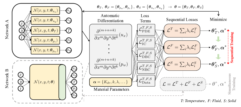
Figure 1: PINN–THM network architecture schematic. Two network types can be used: (A) separate networks for each solution variable (no parameter sharing), and (B) a single network with multiple outputs (shared parameters). The yellow colored boxes present the network parameters. Differential operators are evaluated using the automatic differentiation algorithm. Characterization parameters are listed in the trainable weights $\boldsymbol{\alpha}$. The loss residuals associated with the temperature (T), fluid (F), and solid (S) governing differential equations ($\mathcal{L}^{T,F,S}_{\text{PDE}}$), Dirichlet ($\mathcal{L}^{T,F,S}_{\text{DBC}}$) and Neumann ($\mathcal{L}^{T,F,S}_{\text{NBC}}$) boundary conditions, initial condition ($\mathcal{L}^{T,F,S}_{\text{IC}}$), and data ($\mathcal{L}^{T,F,S}_{\text{Data}}$) are evaluated on sampling points ($\textbf{X},\textbf{Y},\textbf{T}$). The temperature, fluid, and solid total losses $\mathcal{L}^{T,F,S}$ are finally evaluated as the weighted summation of individual loss terms. Minimizing the total loss results in the optimal network parameters. Sequential and simultaneous training strategies can be used. However, using network architecture A becomes mandatory for the sequential training strategy, in order to freeze one network during sequential iterations.

The PINN–THM network architecture is shown schematically in Fig. 1. Two network architectures can be used in general. Separate networks for each solution variable (Network A) or a single network with multiple outputs (Network B). We have explored these architectures in the past and found Network A to be a better strategy (see [31, 32] for details). Additionally, for a sequential training strategy, Network A becomes the only choice because one can freeze any set of parameters during sequential iterations. The trainable parameters of the PDEs (those that we are interested in characterizing given data) are listed in $\boldsymbol{\alpha}$. The automatic differentiation algorithm is used to evaluate differential operators on each solution variable. The loss terms are then evaluated on the collocation points $\textbf{X},\textbf{Y},\textbf{T}$. Total loss is then evaluated as the weighted summation of the individual loss terms. We explored, in details, different adaptive weight schemes for the PINN–THM solver [32] and found that GradNorm [17] results in the best accuracy and therefore is used in this study. The optimization is then performed using the ADAM optimizer.

We leverage the stress-split sequential optimization strategy proposed in [32, 4]. To this end, we first optimize for temperature field by freezing the displacement and pressure networks. We then use the temperature results to optimize for the pressure network. We finally optimize for displacements given temperature and fluid pressure distributions using the fixed-stress operator split formulation [48, 49]. We repeat this sequence until convergence. The algorithm searches for optimal network parameters as well as PDE parameters simultaneously. Therefore, the forward and inverse solvers remain almost identical—a clear advantage of PINN solvers. Accordingly, the sequential optimization problem can be summarized as:

$$\boldsymbol{\theta}_{T}^{i+1},\boldsymbol{\alpha}^{i+1}=\operatorname*{arg\,min}_{\boldsymbol{\theta}_{T},\boldsymbol{\alpha}}\mathcal{L}_{T}(\mathbf{X},\mathbf{Y},\mathbf{T},\bar{T};\hat{P}_{w}^{i},\hat{P}_{c}^{i},\hat{U}_{x}^{i},\hat{U}_{y}^{i},\boldsymbol{\alpha}^{i}),$$ (36)

$$\boldsymbol{\theta}_{F}^{i+1},\boldsymbol{\alpha}^{i+1}=\operatorname*{arg\,min}_{\boldsymbol{\theta}_{p_{w},p_{c}},\boldsymbol{\alpha}}\mathcal{L}_{F}(\mathbf{X},\mathbf{Y},\mathbf{T},\bar{P}_{w};\hat{T}^{i+1},\hat{U}_{x}^{i},\hat{U}_{y}^{i},\boldsymbol{\alpha}^{i+1}),$$ (37)

$$\boldsymbol{\theta}_{S}^{i+1},\boldsymbol{\alpha}^{i+1}=\operatorname*{arg\,min}_{\boldsymbol{\theta}_{S},\boldsymbol{\alpha}}\mathcal{L}_{S}(\mathbf{X},\mathbf{Y},\mathbf{T},\bar{U}_{x},\bar{U}_{y};\hat{T}^{i+1},\hat{P}_{w}^{i+1},\hat{P}_{c}^{i+1},\boldsymbol{\alpha}^{i+1}),$$ (38)

where, subscripts $T,F,S$ stand for thermal, fluid, and solid terms of the loss and network parameters, and $i$ represents the sequential iteration loop. The overbar terms $\bar{T},\bar{P_{w}},\bar{U}_{x},\bar{U_{y}}$ highlight any given data for the inverse solver. The vectors $\hat{T},\hat{P}_{w},\hat{P}_{c},\hat{U_{x}},\hat{U}_{y}$ represent the approximate network outputs at collocation points $\mathbf{X},\mathbf{Y},\mathbf{T}$, getting updated during sequential iterations. Note that compared to PINN forward solvers, PDE parameters, listed in $\boldsymbol{\alpha}$, are also trainable for an inverse solver and are optimized during the optimization. Here, we form the loss functions using the dimensionless relations (28)–(34).

Even though some problems, such as Terzaghi’s consolidation problem, are one-way coupled in their forward setup, they still require sequential iterations in their inverse analysis since their characteristic parameters are altered by all coupled processes.

4 Applications

In this section, we evaluate the performance of the proposed PINN inverse solver for the consolidation problem under (i) isothermal and (ii) nonisothermal conditions, and (iii) the Barry-Mercer’s injection-production problem. The parameters for characterization include permeability ${\bar{k}}$, drained bulk modulus ${\bar{K}_{dr}}$ and thermal conductivity ${\bar{\lambda}}$. We assume that Poison’s ratio is known a priori; therefore, one can evaluate Young’s modulus using isotropic elasticity relations. Since these are normalized variables, we select their initial values as 2, with their expected target values from optimization as 1. The dimensional form of these variables are, however, important ultimately and are calculated using relations (28).

With regard to the network and optimization hyper-parameters and implementation details, we use the ADAM optimizer of TensorFlow/Keras package using the SciANN API [30]. The batch size is set to 500 and each sequential training is performed using 5,000 epochs.

4.1 Terzaghi’s Consolidation Problem

As the first example, let us consider the one-dimensional Terzaghi’s consolidation problem. Consider a soil column of length $L=50$ m, constrained laterally and at the bottom, with no-flux condition on all sides except for the top face. The sample has a Young modulus $120~{}\text{MPa}$, drained Poisson’s ratio $0.25$, Biot coefficient $1.0$, and permeability of $10^{-12}~{}\mathrm{m}^{2}$. The sample is suddenly subjected to an overburden stress $q=0.1~{}\text{MPa}$. The Biot’s bulk modulus, ${M}$, expressed as $M^{-1}=\phi_{0}c_{f}+({b-\phi_{0}})/{K_{s}}$, is taken as $3\times 10^{5}~{}\text{MPa}$. The one-dimensional single phase governing relations are therefore written as:

$$\left(\frac{b^{2}}{\bar{K}_{dr}}+\frac{1}{\bar{M}}\right){D^{*}}\frac{\partial\bar{p}}{\partial\bar{t}}-{\frac{\bar{k}}{\bar{\mu}}}\frac{\partial^{2}\bar{p}}{\partial\bar{y}^{2}}=0,$$ (39)

$${\bar{K}_{dr}}\frac{\partial\bar{\varepsilon}_{v}}{\partial\bar{y}}+{\frac{1}{2}}\left({\frac{1-2\nu}{1+\nu}}\right){\bar{K}_{dr}}\frac{\partial^{2}\bar{u}}{\partial\bar{y}^{2}}+{\frac{3}{2}}\left({\frac{1-2\nu}{1+\nu}}\right){\bar{K}_{dr}}\frac{\partial^{2}\bar{u}}{\partial\bar{y}^{2}}-{b}\frac{\partial\bar{p}}{\partial\bar{y}}=0.$$ (40)

Here, we consider that the pressure and displacement data are given at two locations, one in the middle of the column for pressure, and another at the top for displacement, as shown in Fig. 2. The displacement and pressure networks are 100 neurons wide, each with 4 hidden layers and with hyperbolic-tangent activation function. A structured sampling grid of 41$\times$101 is used to train the problem.

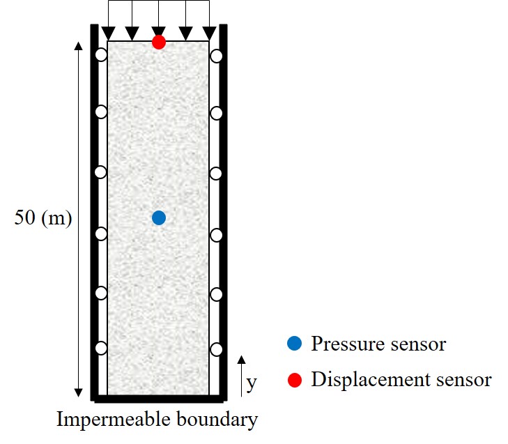
Figure 2: Terzaghi’s consolidation problem; geometry, boundary conditions, and location of pressure (blue) and displacement (red) sensors.

The results for displacement and pressure distributions are shown in Fig. 3, and the parameter identification results are plotted in Fig. 4 with each vertical line highlighting the sequential iterations. Following the forward PINN–Poroelasticity solver [32], we first invert for fluid flow, then use the output pressure to invert for solid deformation. Since parameters are unknown a priori, every sequential iteration may alter both solution variables and PDE parameters until convergence is reached.

As illustrated in Fig. 4, the permeability is first under-estimated due to the lack of information for the drained bulk modulus. With more accurate information on the drained bulk modulus, as a result of solving the solid PDE given the pressure distribution, this error is corrected during the following sequential iterations. The results show the remarkable performance of the sequential PINN solver for parameter identification in Terzaghi’s consolidation problem.

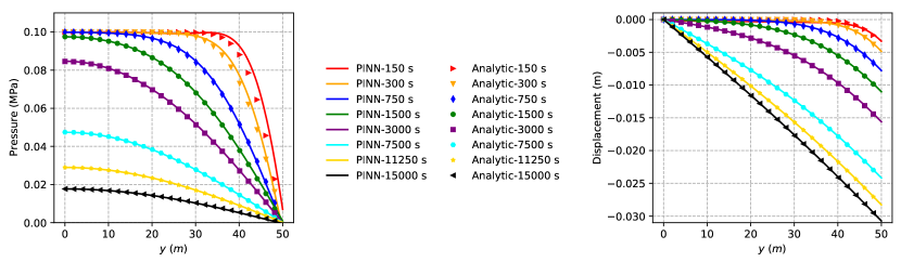
Figure 3: Terzaghi’s consolidation problem; (Left) PINN’s pressure solution, and (Right) PINN’s displacement solution at different time steps, compared against the analytical solution.

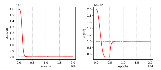
Figure 4: Terzaghi’s consolidation problem; The characterization results (inverse solution) for bulk compressibility ${K_{dr}}$ and permeability ${k}$, as a function of training epochs, with vertical lines highlighting the sequential iterations.

4.2 Barry–Mercer’s Injection–Production Problem

As the second example, we characterize the drained bulk modulus and the permeability of a rectangular domain, subjected to a time-dependent point fluid injection–production, known as Barry–Mercer problem [6]. We use the setup of [62, 63], with the injection/production well located at ${(x_{0},y_{0})=(0.25,0.25)}$, inside a two-dimensional domain of length and width as ${a=b=1\text{m}}$. The solid and fluid phases are incompressible, the Biot coefficient is ${b=1}$, the elastic modulus and Poisson ratio are ${E=4.67~{}\text{MPa}}$ and ${\nu=0.167}$, respectively, and the initial pressure and displacement are set to zero.

The injection/production function $f(t)$ is given as:

$$f(t)={2\beta}{\delta(x-x_{0})\delta(y-y_{0})}{\sin(\beta t)},$$ (41)

with $\beta=0.5~{}\text{s}^{-1}$, that is associated with ${k=10^{-10}~{}\text{m}^{2}}$ and ${\mu=10^{-3}~{}\text{Pa.s}}$, given ${\beta}$’s definition [62, 63, 32]. The Dirac delta function ${\delta}$ is approximated as ${\delta(x)}=\frac{1}{\alpha\sqrt{\pi}}{e^{-(x/\alpha)^{2}}}$, where we use ${\alpha=0.04}$. Similar to Barry and Mercer [6], we normalize the temporal domain by defining ${\hat{t}=\beta t}$, where ${\hat{t}\in[0,2\pi]}$ is the dimensionless time. The single-phase two-way coupled HM governing equations are then summarized as:

$$\frac{b^{2}}{\bar{K}_{dr}}{D^{*}}\frac{\partial\bar{p}}{\partial\bar{t}}+\frac{b}{\bar{K}_{dr}}{D^{*}}\frac{\partial\bar{\sigma}_{v}}{\partial\bar{t}}-{\frac{\bar{k}}{\bar{\mu}}}\bar{\boldsymbol{\nabla}}^{2}\bar{p}-{f^{*}}=0,$$ (42)

$${\bar{K}_{dr}}\boldsymbol{\bar{\nabla}}{\bar{\varepsilon}_{v}}+{\frac{1}{2}}\left({\frac{1-2\nu}{1+\nu}}\right){\bar{K}_{dr}}{\boldsymbol{\bar{\nabla}}}{(\boldsymbol{\bar{\nabla}}{\cdot}{\boldsymbol{\bar{u}}})}+{\frac{3}{2}}\left({\frac{1-2\nu}{1+\nu}}\right){\bar{K}_{dr}}{\boldsymbol{\bar{\nabla}}}{\cdot}{(\boldsymbol{\bar{\nabla}}{\boldsymbol{\bar{u}}})}-{b}{\boldsymbol{\bar{\nabla}}}{{\bar{p}}}=\boldsymbol{0}.$$ (43)

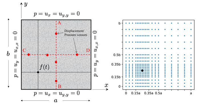
Figure 5: Barry–Mercer’s injection–production problem. All edges are subjected to zero-pressure condition, and they are fixed in their normal direction. A production/injection source term $f(t)$ is applied at $(x_{0},y_{0})$. Red points, located at $0.1,~{}0.4,~{}\text{and}~{}0.8$ relative to a and b, along AB and CD lines represent the location of the sensors providing pressure and displacement data. The collocation grid is shown in blue in the right figure. Due to the type of the injection/production delta function, we use a finer grid around the well location.

Although not restrictive, we assume that vertical and horizontal displacements, as well as pore pressure, are given at a total of 6 sensors located along AB and CD lines shown in Fig. 5. Additionally, since the injection and production source term is calculated based on a sharp Gaussian approximation of the Dirac delta function, with its spike localized near the injection well, we found that using more collocation points near the injection well increases the accuracy of the PINN solver. In Fig. 6 we present the obtained pressure and displacements at $(0.25,0.75)m$, $(0.75,0.75)m$, and $(0.75,0.25)~{}m$, all away from the AB and CD lines where sensor data are provided, and the results match the expected analytical curves remarkably well. The evolution of the inversion parameters are plotted in Fig. 7, with vertical lines highlighting the epoch of sequential iterations. Again, the first sequential iteration has the highest error, with each sequential iteration resulting in improved accuracy, until reaching very high accuracy at the fifth iteration of sequential training. The displacement and pressure networks are 100 neurons wide, each with 4 hidden layers and with hyperbolic-tangent activation function and with Fourier features. A structured sampling grid of 21$\times$21$\times$41 is used to train the problem.

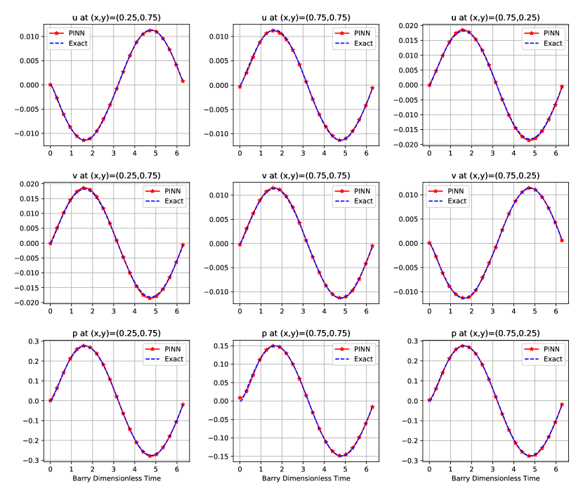
Figure 6: Barry–Mercer’s PINN solution; (Top) horizontal displacement; (Middle) vertical displacement; (Bottom) pore pressure. Each column represent a different location away from the injection–production well.

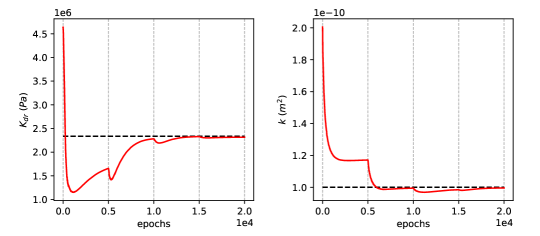
Figure 7: Barry–Mercer’s solution; evolution of characterization of bulk compressibility ${K_{dr}}$ and permeability ${k}$ as a function of training epochs, with vertical lines highlighting the sequential iterations.

4.3 Thermoelastic Consolidation of Unsaturated Stratum

As the last example, we consider a fully coupled THM problem under nonisothermal conditions: nonisothermal consolidation through an unsaturated elastic stratum. Here, we aim to characterize the drained bulk modulus $K_{dr}$, the permeability $k$, and the thermal conductivity $\lambda_{\text{avg}}$, under nonisothermal two-phase fluid flow. Many studies, including Dakshanamurthy and Fredlund [21], Gawin et al. [28], Schrefler et al. [69], and recently Khoei et al. [47] solved the forward problem under various conditions, including isothermal/nonisothermal, swelling/consolidation, and considering/ignoring the effect of phase change. We also recently solved the forward problem using PINNs [4], and here we address the inverse problem for the first time.

The problem setup is based on Khoei et al. [47], as follows. A ${{10}~{}\text{cm}}$ stratum with initial conditions of ${{p_{c}=280}~{}\text{kPa}}$, ${{p_{g}=102}~{}\text{kPa}}$, ${{T=10}~{}{{}^{\circ}}\text{C}}$ is subjected to ${{15}~{}{{}^{\circ}}\text{C}}$ and ${{140}~{}\text{kPa}}$ increase in temperature and capillary pressure, respectively. The boundary conditions of the top surface are ${{p_{c}=420}~{}\text{kPa}}$, ${{p_{g}=102}~{}\text{kPa}}$, and ${{T=25}~{}{{}^{\circ}}\text{C}}$. The bottom surface is impermeable to heat transfer and fluid flow, and has fixed displacements.

Material properties include the Young modulus ${E=60~{}\text{MPa}}$, the Poisson ratio ${{\nu}={0.2857}}$, the porosity ${\phi=0.5}$, and Biot modulus ${b=1}$. The bulk moduli are considered as ${K_{s}}=0.14\times 10^{10}~{}\text{Pa}$, ${K_{w}}=0.43\times 10^{13}~{}\text{Pa}$, and $K_{g}=0.1\times 10^{6}~{}\text{Pa}$ for solid, water, and gas phases, respectively. The fluid flow parameters are taken as $k={6}{\times}{10^{-15}~{}{\text{m}^{2}}}$ and ${\mu_{w}}={\mu_{g}}={10^{-3}}~{}{\text{Pa}\cdot\text{s}}$. The densities are ${\rho_{s}}={1800}~{}{\text{kg}/\text{m}^{3}}$, ${\rho_{w}}={1000}~{}{\text{kg}/\text{m}^{3}}$, and ${\rho_{g}}={1.22}~{}{\text{kg}/\text{m}^{3}}$. The thermal conductivity coefficient is considered as ${\lambda_{\text{avg}}}={0.458}~{}{\text{J}/\text{s}\cdot\text{m}\cdot{{}^{\circ}}\text{C}}$, with the heat capacity as ${C_{s}}={125460}~{}{\text{J}/\text{kg}\cdot{{}^{\circ}}\text{C}}$, ${C_{w}}={4182}~{}{\text{J}/\text{kg}\cdot{{}^{\circ}}\text{C}}$, and ${C_{g}}={1000}~{}{\text{J}/\text{kg}\cdot{{}^{\circ}}\text{C}}$. In addition, the thermal expansion coefficients are given as ${\beta_{s}}={9}{\times}{10^{-7}}~{}{1/{{}^{\circ}}\text{C}}$, ${\beta_{w}}={6.3}{\times}{10^{-6}}~{}{1/{{}^{\circ}}\text{C}}$, and ${\beta_{g}}={3.3}{\times}{10^{-3}}~{}{1/{{}^{\circ}}\text{C}}$. To describe the flow of two immiscible fluids through the porous medium, the Brooks–Corey [12] relations for capillary pressure and relative permeability of the fluid phases are used, as:

$${p_{c}}={p_{b}}{S_{e}}^{-1/\lambda},\quad{k_{rw}}={S_{e}}^{(2+3\lambda)/\lambda},\quad{k_{rg}}={(1-{S_{e}})^{2}}{(1-{S_{e}}^{(2+\lambda)/\lambda})},\quad{S_{e}}={\frac{S_{w}-S_{rw}}{1-{S_{rw}}}},$$ (44)

in which ${S_{e}}$ denotes the effective saturation, and ${k_{rw}}$ and ${k_{rg}}$ are the relative permeabilities of water and gas phases, respectively. Finally, the pore size distribution and the residual water saturation parameters are ${\lambda=2.308}$ and ${S_{rw}=0.3216}$, respectively, and the capillary entry pressure is taken as ${{p_{b}=133.813}~{}\text{kPa}}$.

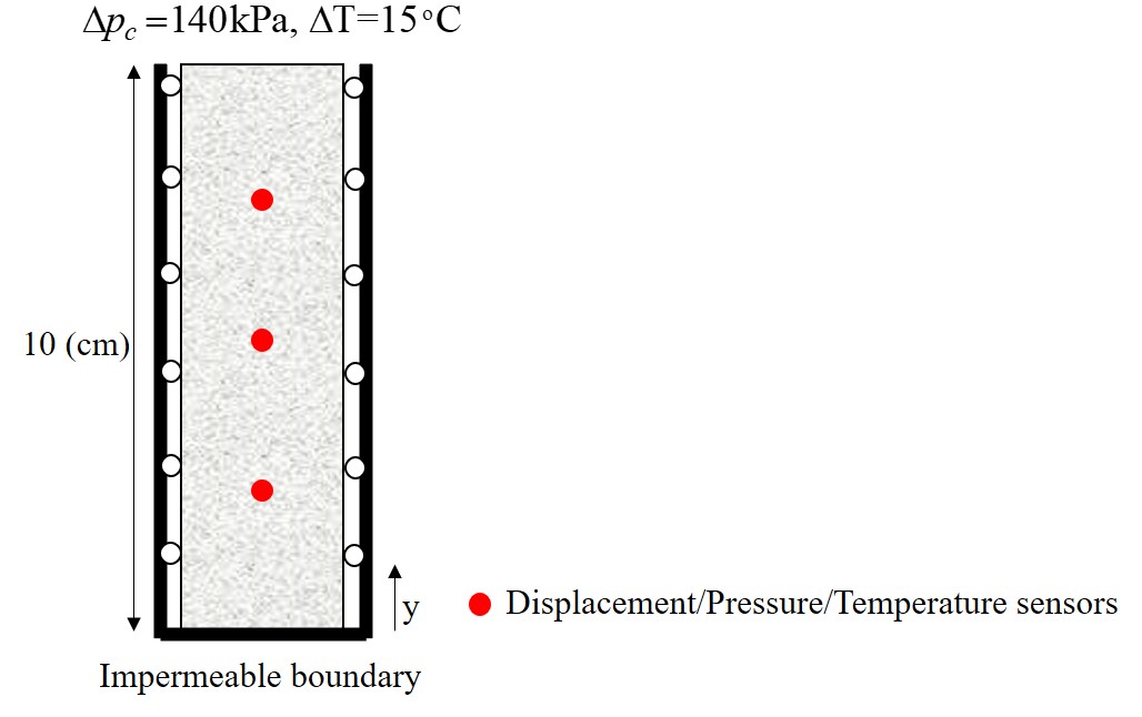
Figure 8: Thermoelastic consolidation of an unsaturated stratum; geometry, boundary conditions and sensor locations are highlighted in the figure.

Given the problem setup and material properties, we take the forward FEM solution for capillary pressure, displacement, and temperature from Khoei et al. [47], at the first, second, and third quarter of the stratum height, as shown in Fig. 8 as the “sensor” data. Given this data, we then attempt to identify the permeability, drained bulk modulus, and thermal conductivity of the stratum using the proposed inverse PINN–THM solver. With the mentioned material properties, the gas pressure variation is about 20 Pa, which is negligible in comparison to capillary and water pressure. Hence, we turn the general format of the equations into a form compatible for passive gas pressure in two-phase fluid flow systems [57, 67]. Therefore, given the constant gas pressure assumption, we can remove the gas fluid flow equation and only consider the capillary pressure as the main functional for the fluid flow, so the water pressure is defined based on the relation Eq. 20. Henceforth, the final form of the formulation used for this problem is expressed as:

$$\begin{split}&{\bar{K}_{dr}}\frac{\partial\bar{\varepsilon}_{v}}{\partial{\bar{y}}}+{2}\left({\frac{1-2\nu}{1+\nu}}\right){\bar{K}_{dr}}\frac{\partial^{2}\bar{u}}{\partial\bar{y}^{2}}-{b}{\sum_{\alpha}}\frac{\partial}{\partial\bar{y}}{({S_{\alpha}}{\bar{p}_{\alpha}})}-{\bar{\beta}_{s}}{\bar{K}_{dr}}{N_{T}}\frac{\partial\bar{T}}{\partial\bar{y}}={0},\end{split}$$ (45)

$$\begin{split}&-\frac{\bar{\mu}_{w}}{\bar{k}}{({\bar{N}_{ww}}+\frac{b_{w}b_{w}}{\bar{K}_{dr}}){D^{*}}{\frac{\partial\bar{p}_{c}}{\partial\bar{t}}}}+\frac{\bar{\mu}_{w}}{\bar{k}}{\frac{bS_{w}}{\bar{K}_{dr}}}{D^{*}}\frac{\partial\bar{\sigma}_{v}}{\partial\bar{t}}-\frac{\bar{\mu}_{w}}{\bar{k}}{\phi S_{w}}\left({\bar{\beta}_{w}}-{\bar{\beta}_{s}}\right){Q^{*}}\frac{\partial\bar{T}}{\partial\bar{t}}\\ &~{}~{}~{}~{}~{}~{}~{}~{}~{}~{}~{}~{}~{}~{}~{}~{}~{}~{}-\frac{\partial}{\partial\bar{y}}{{\left({k_{w}^{r}}\frac{\partial\bar{p}_{w}}{\partial\bar{y}}\right)}}={{0}},\end{split}$$ (46)

$${H^{*}}{\frac{\partial\bar{T}}{\partial\bar{t}}}-{J^{*}}{\left({\bar{\rho}_{w}}{\bar{C}_{w}}{k^{r}_{w}}\frac{\bar{k}}{\bar{\mu}_{w}}\frac{\partial\bar{p}_{w}}{\partial\bar{y}}\right)}\frac{\partial\bar{T}}{\partial\bar{y}}-{F^{*}}\frac{\partial}{\partial\bar{y}}{({{\bar{\lambda}_{\text{avg}}}}\frac{\partial\bar{T}}{\partial\bar{y}})}={0}.$$ (47)

By experimentation, we also realized that for characterization of permeability in this two-phase flow example, multiplying the fluid flow governing equation by ${\bar{\mu}_{w}}/{\bar{k}}$ results in more accurate parameters, i.e., Eq. 46. We associated this to the small diffusion term in the flow relation as a result of small value for ${k^{r}_{w}}$. Regarding the neural network hyperparameters, the displacement, pressure, and temperature networks are all built with 40 neurons width and with 8 hidden layers and tangent-hyperbolic activation function. A structured sampling grid of 41$\times$100 is used to train the problem.

The results of the sequential PINN–THM inverse solver are shown in Figs. 9 and 10. With initial values far from their true values, we find that the proposed solver results in highly accurate temperature, displacement, and capillary pressure spatio-temporal distributions compared with FEM results, as shown in Fig. 9. The evolution of the estimated parameter values, shown in Fig. 10, additionally highlights the success of sequential training for this complex inverse problem. Compared to the previous problems, this example exhibited the highest sensitivity with respect to the medium fluid-flow permeability and to the choices of optimization hyperparameters such as learning rate—a finding that is not entirely surprising given the complexity and nonlinearity of the coupled PDEs.

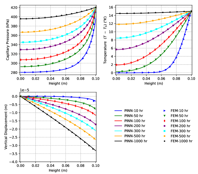
Figure 9: Thermoelastic consolidation of an unsaturated stratum; PINN solutions, i.e., capillary pressure, temperature, and vertical displacement (solid lines) and comparison against the FEM solutions reported by Khoei et al. [47] (symbols). The horizontal axis indicates the depth of the stratum. Different colors show the solution at different times.

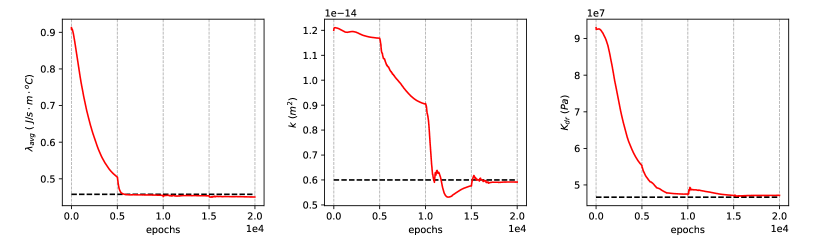
Figure 10: Thermoelastic consolidation of an unsaturated stratum; the evolution of characterization of average thermal conductivity $\lambda_{\text{avg}}$, permeability ${k}$, and bulk compressibility ${K_{dr}}$parameters evolution as a function of training epochs, with vertical lines highlighting the sequential iterations.

5 Conclusions

We investigated the application of sequential PINN–THM for the characterization of deforming fully and partially saturated porous media under isothermal and nonisothermal conditions. The proposed PINN framework features a dimensionless form of the THM governing PDEs suitable for inverse analysis, a sequential training strategy for the multi-physics THM processes in porous media, and adaptive weight methods to prevent unbalance convergence of loss terms. We validated our proposed framework on three reference problems of porous media, and reported remarkable performance of PINNs to simultaneously capture the solution variables and identify the PDE parameters.

Model inversion using classical methods is a nontrivial and computationally expensive task. Classical solvers such as FEM and FVM are well suited to simulate forward problems but an external optimization loop is needed to perform inversion. Each iteration of the optimization requires loss and gradient evaluation and, therefore, multiple forward solves are needed per optimization iteration to perform a parameter update. The inversion optimization can also suffer from the complex loss landscape associated with multidimensional, coupled and highly nonlinear PDEs. In this respect, the main advantage of PINN solvers is that they can be used for simultaneous forward and inverse modeling, as data incorporation, loss and gradient evaluations are naturally a part of PINN solvers. Therefore, while in general the performance of PINN forward solvers is far from optimal, we find that as inverse solvers they can in fact be competitive. Substantial performance improvements, however, are likely as PINN network architectures and optimization strategies continue to evolve.

The applications of our proposed PINN–THM inversion framework have so far been limited to synthetic problems on simple geometries. In the future, we plan to apply the framework to more complex problems with real-world, multifaceted datasets.

Data availability statement

All data, models, or code generated or used during the study are available in a repository online (https://github.com/sciann/sciann-applications/tree/master/SciANN-PoroElasticity) in accordance with funder data retention policies.

References

- Abadi et al. [2016] Martín Abadi, Paul Barham, Jianmin Chen, Zhifeng Chen, Andy Davis, Jeffrey Dean, Matthieu Devin, Sanjay Ghemawat, Geoffrey Irving, Michael Isard, et al. TensorFlow: a system for large-scale machine learning. In 12th USENIX symposium on operating systems design and implementation (OSDI 16), pages 265–283, 2016.
- Alghamdi et al. [2020] Amal Alghamdi, Marc A Hesse, Jingyi Chen, and Omar Ghattas. Bayesian poroelastic aquifer characterization from insar surface deformation data. part i: Maximum a posteriori estimate. Water Resources Research, 56(10):e2020WR027391, 2020.
- Almajid and Abu-Alsaud [2021] Muhammad M Almajid and Moataz O Abu-Alsaud. Prediction of porous media fluid flow using physics informed neural networks. Journal of Petroleum Science and Engineering, 208:109205, 2021.
- Amini et al. [2022] Danial Amini, Ehsan Haghighat, and Ruben Juanes. Physics-informed neural network solution of thermo-hydro-mechanical (THM) processes in porous media. Journal of Engineering Mechanics, 2022.
- Armero [1999] Francisco Armero. Formulation and finite element implementation of a multiplicative model of coupled poro-plasticity at finite strains under fully saturated conditions. Computer Methods in Applied Mechanics and Engineering, 171(3-4):205–241, 1999.
- Barry and Mercer [1999] S. I. Barry and G. N. Mercer. Exact Solutions for Two-Dimensional Time-Dependent Flow and Deformation Within a Poroelastic Medium. Journal of Applied Mechanics, 66(2):536–540, 1999.
- Baydin et al. [2017] A. G. Baydin, B. A. Pearlmutter, A. A. Radul, and J. M. Siskind. Automatic differentiation in machine learning: a survey. Journal of Machine Learning Research, 18(1):5595–5637, 2017.
- Bekele [2020] Yared W Bekele. Physics-informed deep learning for flow and deformation in poroelastic media. arXiv preprint arXiv:2010.15426, 2020.
- Bekele [2021] Yared W Bekele. Physics-informed deep learning for one-dimensional consolidation. Journal of Rock Mechanics and Geotechnical Engineering, 13(2):420–430, 2021.
- Bense et al. [2013] V. F. Bense, T. Gleeson, S. E. Loveless, O. Bour, and J. Scibek. Fault zone hydrogeology. Earth-Science Reviews, 127:171–192, 2013.
- Biot [1941] Maurice A Biot. General theory of three-dimensional consolidation. Journal of Applied Physics, 12(2):155–164, 1941.
- Brooks and Corey [1966] Royal Harvard Brooks and Arthur T Corey. Properties of porous media affecting fluid flow. Journal of the Irrigation and Drainage Division, 92(2):61–88, 1966.
- Cai et al. [2021] Shengze Cai, Zhicheng Wang, Sifan Wang, Paris Perdikaris, and George Em Karniadakis. Physics-informed neural networks for heat transfer problems. Journal of Heat Transfer, 143(6):060801, 2021.
- Cai et al. [2022] Shengze Cai, Zhiping Mao, Zhicheng Wang, Minglang Yin, and George Em Karniadakis. Physics-informed neural networks (PINNs) for fluid mechanics: A review. Acta Mechanica Sinica, pages 1–12, 2022.
- Carrera and Neuman [1986] J. Carrera and S. P. Neuman. Estimation of aquifer parameters under transient and steady state conditions: 1. Maximum likelihood method incorporating prior information. Water Resources Research, 22(2):199—210, 1986.
- Carrera et al. [2005] J. Carrera, A. Alcolea, A. Medina, J. Hidalgo, and L. J. Slooten. Inverse problem in hydrogeology. Hydrogeol. J., 13(1):206–222, 2005.
- Chen et al. [2018] Zhao Chen, Vijay Badrinarayanan, Chen-Yu Lee, and Andrew Rabinovich. Gradnorm: Gradient normalization for adaptive loss balancing in deep multitask networks. In International Conference on Machine Learning, pages 794–803. PMLR, 2018.
- Coussy [2004] Olivier Coussy. Poromechanics. John Wiley & Sons, 2004.
- Cui et al. [2014] T. Cui, J. Martin, Y. M. Marzouk, A. Solonen, and A. Spantini. Likelihood-informed dimension reduction for nonlinear inverse problems. Inverse Problems, 30(11):114015, 2014.
- Cuomo et al. [2022] Salvatore Cuomo, Vincenzo Schiano Di Cola, Fabio Giampaolo, Gianluigi Rozza, Maizar Raissi, and Francesco Piccialli. Scientific machine learning through physics-informed neural networks: Where we are and what’s next. Journal of Scientific Computing, 92(3):88, 2022.
- Dakshanamurthy and Fredlund [1981] V Dakshanamurthy and DG Fredlund. A mathematical model for predicting moisture flow in an unsaturated soil under hydraulic and temperature gradients. Water Resources Research, 17(3):714–722, 1981.
- Ellsworth [2013] W. L. Ellsworth. Injection-induced earthquakes. Science, 341:1225942, 2013.
- Fraces and Tchelepi [2021] Cedric G Fraces and Hamdi Tchelepi. Physics informed deep learning for flow and transport in porous media. In SPE Reservoir Simulation Conference, pages SPE–203934–MS. OnePetro, 2021.
- Fraces et al. [2020] Cedric G Fraces, Adrien Papaioannou, and Hamdi Tchelepi. Physics informed deep learning for transport in porous media. Buckley Leverett problem. arXiv preprint arXiv:2001.05172, 2020.
- Fuks and Tchelepi [2020] Olga Fuks and Hamdi A Tchelepi. Limitations of physics informed machine learning for nonlinear two-phase transport in porous media. Journal of Machine Learning for Modeling and Computing, 1(1):19–37, 2020.
- Gabrielli et al. [2020] P. Gabrielli, A. Poluzzi, G. J. Kramer, C. Spiers, M. Mazzotti, and M. Gazzani. Seasonal energy storage for zero-emissions multi-energy systems via underground hydrogen storage. Renewable and Sustainable Energy Reviews, 121:109629, 2020.
- Galloway and Burbey [2011] D. L. Galloway and T. J. Burbey. Regional land subsidence accompanying groundwater extraction. Hydrogeology Journal, 19(8):1459–1486, 2011.
- Gawin et al. [1996] Dariusz Gawin, Bernhard A Schrefler, and M Galindo. Thermo-hydro-mechanical analysis of partially saturated porous materials. Engineering Computations, 13(7):113–143, 1996.
- Gorelick and Zheng [2015] S. M. Gorelick and C. Zheng. Global change and the groundwater management challenge. Water Resources Research, 51(5):3031–3051, 2015.
- Haghighat and Juanes [2021] Ehsan Haghighat and Ruben Juanes. SciANN: A Keras/TensorFlow wrapper for scientific computations and physics-informed deep learning using artificial neural networks. Computer Methods in Applied Mechanics and Engineering, 373:113552, 2021.
- Haghighat et al. [2021] Ehsan Haghighat, Maziar Raissi, Adrian Moure, Hector Gomez, and Ruben Juanes. A physics-informed deep learning framework for inversion and surrogate modeling in solid mechanics. Computer Methods in Applied Mechanics and Engineering, 379:113741, 2021.
- Haghighat et al. [2022] Ehsan Haghighat, Danial Amini, and Ruben Juanes. Physics-informed neural network simulation of multiphase poroelasticity using stress-split sequential training. Computer Methods in Applied Mechanics and Engineering, 397:115141, 2022.
- Harp et al. [2021] Dylan Robert Harp, Dan O’Malley, Bicheng Yan, and Rajesh Pawar. On the feasibility of using physics-informed machine learning for underground reservoir pressure management. Expert Systems with Applications, 178:115006, 2021.
- Hesse and Stadler [2014] Marc A Hesse and Georg Stadler. Joint inversion in coupled quasi-static poroelasticity. Journal of Geophysical Research: Solid Earth, 119(2):1425–1445, 2014.
- Iglesias and McLaughlin [2012] Marco A Iglesias and Dennis McLaughlin. Data inversion in coupled subsurface flow and geomechanics models. Inverse Problems, 28(11):115009, 2012.
- IPCC [2005] IPCC. Special Report on Carbon Dioxide Capture and Storage, B. Metz et al. (eds.). Cambridge University Press, 2005.
- Jagtap and Karniadakis [2020] Ameya D Jagtap and George Em Karniadakis. Extended physics-informed neural networks (xPINNs): A generalized space-time domain decomposition based deep learning framework for nonlinear partial differential equations. Communications in Computational Physics, 28(5):2002–2041, 2020.
- Jagtap et al. [2020] Ameya D Jagtap, Ehsan Kharazmi, and George Em Karniadakis. Conservative physics-informed neural networks on discrete domains for conservation laws: Applications to forward and inverse problems. Computer Methods in Applied Mechanics and Engineering, 365:113028, 2020.
- Jha and Juanes [2007] Birendra Jha and Ruben Juanes. A locally conservative finite element framework for the simulation of coupled flow and reservoir geomechanics. Acta Geotechnica, 2(3):139–153, 2007.
- Jha and Juanes [2014] Birendra Jha and Ruben Juanes. Coupled multiphase flow and poromechanics: A computational model of pore pressure effects on fault slip and earthquake triggering. Water Resources Research, 50(5):3776–3808, 2014.
- Jha et al. [2015] Birendra Jha, Francesca Bottazzi, Rafal Wojcik, Martina Coccia, Noah Bechor, Dennis McLaughlin, Thomas Herring, Bradford H Hager, Stefano Mantica, and Ruben Juanes. Reservoir characterization in an underground gas storage field using joint inversion of flow and geodetic data. International Journal for Numerical and Analytical Methods in Geomechanics, 39(14):1619–1638, 2015.
- Jin et al. [2021] Xiaowei Jin, Shengze Cai, Hui Li, and George Em Karniadakis. NSFnets (Navier-Stokes flow nets): Physics-informed neural networks for the incompressible Navier-Stokes equations. Journal of Computational Physics, 426:109951, 2021.
- Kadeethum et al. [2020] T. Kadeethum, T. M. Jørgensen, and H. M. Nick. Physics-informed neural networks for solving nonlinear diffusivity and Biot’s equations. PLoS One, 15(5):e0232683, 2020.
- Kang et al. [2016] P. K. Kang, Y. Zheng, X. Fang, R. Wojcik, D. McLaughlin, S. Brown, M. C. Fehler, D. R. Burns, and R. Juanes. Sequential approach to joint flow-seismic inversion for improved characterization of fractured media. Water Resources Research, 52(2):903–919, 2016.
- Karniadakis et al. [2021] George Em Karniadakis, Ioannis G Kevrekidis, Lu Lu, Paris Perdikaris, Sifan Wang, and Liu Yang. Physics-informed machine learning. Nature Reviews Physics, 3(6):422–440, 2021.
- Keranen et al. [2014] K. M. Keranen, M. Weingarten, G. A. Abers, B. A. Bekins, and S. Ge. Sharp increase in central Oklahoma seismicity since 2008 induced by massive wastewater injection. Science, 345:448–451, 2014.
- Khoei et al. [2021] Amir R Khoei, Danial Amini, and S Mohammad S Mortazavi. Modeling non-isothermal two-phase fluid flow with phase change in deformable fractured porous media using extended finite element method. International Journal for Numerical Methods in Engineering, 122:4378–4426, 2021.
- Kim et al. [2011] Jihoon Kim, Hamdi A Tchelepi, and Ruben Juanes. Stability and convergence of sequential methods for coupled flow and geomechanics: Fixed-stress and fixed-strain splits. Computer Methods in Applied Mechanics and Engineering, 200(13-16):1591–1606, 2011.
- Kim et al. [2013] Jihoon Kim, Hamdi A Tchelepi, and Ruben Juanes. Rigorous coupling of geomechanics and multiphase flow with strong capillarity. SPE Journal, 18(06):1123–1139, 2013.
- Laubscher [2021] Ryno Laubscher. Simulation of multi-species flow and heat transfer using physics-informed neural networks. Physics of Fluids, 33(8):087101, 2021.
- Lewis and Schrefler [1998] Roland W Lewis and BA Schrefler. The finite element method in the static and dynamic deformation and consolidation of porous media. John Wiley & Sons, 1998.
- Lumley [2001] David E Lumley. Time-lapse seismic reservoir monitoring. Geophysics, 66(1):50–53, 2001.
- Mao et al. [2020] Zhiping Mao, Ameya D Jagtap, and George Em Karniadakis. Physics-informed neural networks for high-speed flows. Computer Methods in Applied Mechanics and Engineering, 360:112789, 2020.
- McLaughlin and Townley [1996] D. McLaughlin and L. R. Townley. A reassessment of the groundwater inverse problem. Water Resources Research, 32(5):1131–1161, 1996.
- Millevoi et al. [2022] Caterina Millevoi, Nicolo Spiezia, and Massimiliano Ferronato. On physics-informed neural networks architecture for coupled hydro-poromechanical problems. Available at SSRN 4074416, 2022.
- Milora and Tester [1976] S. L. Milora and J. W. Tester. Geothermal Energy as a Source of Electric Power: Thermodynamic and Economic Design Criteria. MIT Press, 1976.
- Mohammadnejad and Khoei [2013] T Mohammadnejad and AR Khoei. Hydro-mechanical modeling of cohesive crack propagation in multiphase porous media using the extended finite element method. International Journal for Numerical and Analytical Methods in Geomechanics, 37(10):1247–1279, 2013.
- National Research Council [2013] National Research Council. Induced Seismicity Potential in Energy Technologies. National Academy Press, Washington, DC, 2013. http://www.nap.edu/catalog.php?record_id=13355.
- Niaki et al. [2021] Sina Amini Niaki, Ehsan Haghighat, Trevor Campbell, Anoush Poursartip, and Reza Vaziri. Physics-informed neural network for modelling the thermochemical curing process of composite-tool systems during manufacture. Computer Methods in Applied Mechanics and Engineering, 384:113959, 2021.
- Oliver and Chen [2011] Dean S Oliver and Yan Chen. Recent progress on reservoir history matching: a review. Computational Geosciences, 15(1):185–221, 2011.
- Paszke et al. [2019] Adam Paszke, Sam Gross, Francisco Massa, Adam Lerer, James Bradbury, Gregory Chanan, Trevor Killeen, Zeming Lin, Natalia Gimelshein, Luca Antiga, et al. Pytorch: An imperative style, high-performance deep learning library. Advances in Neural Information Processing Systems (NeurIPS 2019), 32, 2019. URL https://proceedings.neurips.cc/paper/2019/file/bdbca288fee7f92f2bfa9f7012727740-Paper.pdf.
- Phillips and Wheeler [2007a] Phillip Joseph Phillips and Mary F Wheeler. A coupling of mixed and continuous galerkin finite element methods for poroelasticity i: the continuous in time case. Computational Geosciences, 11(2):131–144, 2007a.
- Phillips and Wheeler [2007b] Phillip Joseph Phillips and Mary F Wheeler. A coupling of mixed and continuous galerkin finite element methods for poroelasticity ii: the discrete-in-time case. Computational Geosciences, 11(2):145–158, 2007b.
- Raissi et al. [2019] Maziar Raissi, Paris Perdikaris, and George E Karniadakis. Physics-informed neural networks: A deep learning framework for solving forward and inverse problems involving nonlinear partial differential equations. Journal of Computational physics, 378:686–707, 2019.
- Rao et al. [2020] Chengping Rao, Hao Sun, and Yang Liu. Physics-informed deep learning for incompressible laminar flows. Theoretical and Applied Mechanics Letters, 10(3):207–212, 2020.
- Rao et al. [2021] Chengping Rao, Hao Sun, and Yang Liu. Physics-informed deep learning for computational elastodynamics without labeled data. Journal of Engineering Mechanics, 147(8):04021043, 2021.
- Schrefler [2002] BA Schrefler. Mechanics and thermodynamics of saturated/unsaturated porous materials and quantitative solutions. Appl. Mech. Rev., 55(4):351–388, 2002.
- Schrefler [2004] BA Schrefler. Multiphase flow in deforming porous material. International Journal for Numerical Methods in Engineering, 60(1):27–50, 2004.
- Schrefler et al. [1995] Bernard A Schrefler, Xiaoyong Zhan, and Luciano Simoni. A coupled model for water flow, airflow and heat flow in deformable porous media. International Journal of Numerical Methods for Heat & Fluid Flow, 5(6), 1995.
- Settari and Mourits [1998] Antonin Settari and FM Mourits. A coupled reservoir and geomechanical simulation system. SPE Journal, 3(03):219–226, 1998.
- Shokouhi et al. [2021] P. Shokouhi, V. Kumar, S. Prathipati, S. A. Hosseini, C. L. Giles, and D. Kifer. Physics-informed deep learning for prediction of CO2 storage site response. Journal of Contaminant Hydrology, page 103835, 2021.
- Sophocleous [2002] M. Sophocleous. Interactions between groundwater and surface water: the state of the science. Hydrogeology Journal, 10(1):52–67, 2002.
- Szulczewski et al. [2012] M. L. Szulczewski, C. W. MacMinn, H. J. Herzog, and R. Juanes. Lifetime of carbon capture and storage as a climate-change mitigation technology. Proc. Natl. Acad. Sci. U.S.A., 109(14):5185–5189, doi:10.1073/pnas.1115347109, 2012.
- Tartakovsky et al. [2020] Alexandre M Tartakovsky, C Ortiz Marrero, Paris Perdikaris, Guzel D Tartakovsky, and David Barajas-Solano. Physics-informed deep neural networks for learning parameters and constitutive relationships in subsurface flow problems. Water Resources Research, 56(5):e2019WR026731, 2020.
- Thomas et al. [2003] LK Thomas, LY Chin, RG Pierson, and JE Sylte. Coupled geomechanics and reservoir simulation. SPE Journal, 8(04):350–358, 2003.
- Vasco et al. [2001] DW Vasco, Kenzi Karasaki, and Kiyoshi Kishida. A coupled inversion of pressure and surface displacement. Water Resources Research, 37(12):3071–3089, 2001.
- Veil [2002] John A. Veil. Drilling waste management: Past, present, and future. In SPE Annual Technical Conference and Exhibition, pages SPE–77388–MS. OnePetro, 2002.
- Wang [2000] H. F. Wang. Theory of Linear Poroelasticity. Princeton University Press, 2000.
- Wang et al. [2021] Sifan Wang, Yujun Teng, and Paris Perdikaris. Understanding and mitigating gradient pathologies in physics-informed neural networks. SIAM Journal on Scientific Computing, 43(5):A3055–A3081, 2021.
- Wang et al. [2022a] Sifan Wang, Shyam Sankaran, and Paris Perdikaris. Respecting causality is all you need for training physics-informed neural networks. arXiv preprint arXiv:2203.07404, 2022a.
- Wang et al. [2022b] Sifan Wang, Xinling Yu, and Paris Perdikaris. When and why PINNs fail to train: A neural tangent kernel perspective. Journal of Computational Physics, 449:110768, 2022b.
- White and Borja [2008] Joshua A White and Ronaldo I Borja. Stabilized low-order finite elements for coupled solid-deformation/fluid-diffusion and their application to fault zone transients. Computer Methods in Applied Mechanics and Engineering, 197(49-50):4353–4366, 2008.
- Wu et al. [2018] Jin-Long Wu, Heng Xiao, and Eric Paterson. Physics-informed machine learning approach for augmenting turbulence models: A comprehensive framework. Physical Review Fluids, 3(7):074602, 2018.
- Zienkiewicz et al. [1999] O.C. Zienkiewicz, A.H.C. Chan, M. Pastor, B.A. Schrefler, and T. Shiomi. Computational Geomechanics with Special Reference to Earthquake Engineering. Wiley, 1999. ISBN 9780471982852.