Reactmine: a statistical search algorithm for inferring chemical reactions from time series data

Abstract

Inferring chemical reaction networks (CRN) from concentration time series is a challenge encouraged by the growing availability of quantitative temporal data at the cellular level. This motivates the design of algorithms to infer the preponderant reactions between the molecular species observed in a given biochemical process, and build CRN structure and kinetics models. Existing ODE-based inference methods such as SINDy resort to least square regression combined with sparsity-enforcing penalization, such as Lasso. However, we observe that these methods fail to learn sparse models when the input time series are only available in wild type conditions, i.e. without the possibility to play with combinations of zeroes in the initial conditions. We present a CRN inference algorithm which enforces sparsity by inferring reactions in a sequential fashion within a search tree of bounded depth, ranking the inferred reaction candidates according to the variance of their kinetics on their supporting transitions, and re-optimizing the kinetic parameters of the CRN candidates on the whole trace in a final pass. We show that Reactmine succeeds both on simulation data by retrieving hidden CRNs where SINDy fails, and on two real datasets, one of fluorescence videomicroscopy of cell cycle and circadian clock markers, the other one of biomedical measurements of systemic circadian biomarkers possibly acting on clock gene expression in peripheral organs, by inferring preponderant regulations in agreement with previous model-based analyses. The code is available at https://gitlab.inria.fr/julmarti/crninf/ together with introductory notebooks.

1 Introduction

With the automation of biological experiments and the increase of quality of cell measurements, automating the building of mechanistic models from data becomes conceivable and a necessity for many new applications. The structure of such models, e.g. gene regulatory networks (GRN) or chemical reaction networks (CRN), is classically built from an extensive review and compilation of the literature by the modeler. More recently, efforts have been made to develop model learning algorithms to assist modelers in order to partly automate the model building process, in particular when time series measurements are available.

Extensive literature is available in the context of GRN inference or unsupervised learning, partly motivated by knowledge discovery problems, such as presented in the DREAM series of challenges (Stolovitzky et al., 2007), or experiment design (King et al., 2004). A GRN consists in a directed graph $G=(W,E)$ of genes and edges $E_{ij}$ between genes, whenever a gene transcription factor $W_{i}$ binds to the promoter region of target gene $W_{j}$. GRN inference algorithms feature a wide range of machine learning methods, e.g. Decision Trees (Huynh-Thu and Geurts, 2018), Information Theory (Zoppoli et al., 2010) or Gaussian Processes (Aalto et al., 2020).

Less work concerns CRN inference, i.e. the problem of inferring both the structure and kinetics of chemical reactions between some molecular species observed with time series data about their concentrations. The structure of a CRN can be represented by a bipartite directed graph with edges from molecular species vertices to reaction vertices, representing the reactants of a reaction, and edges from reaction vertices to species representing their product. Of note, the indegree and outdegree of a reaction node can be above one, which allows for bimolecular reactions like complexations, e.g. $A+B\rightarrow C$, or catalyzed transformations, e.g. $A+B\rightarrow A+C$. Each reaction of a CRN is given with its kinetics, using reaction rate functions such as mass action law, Michaelis-Menten or Hill kinetics. The rate function of each reaction appears as a term in the ordinary differential equations (ODE) that govern the time evolution of the products and reactants of the reaction. Overall, both the difference of structure and the importance of the kinetics make the above GRN inference methods hardly applicable to CRN inference problems.

CRN inference may thus rely on the ODE semantics of a CRN to apply ODE inference methods from time series data, such as the state-of-the-art tool SINDy (Sparse Identification of Nonlinear Dynamics, Brunton et al. (2016)) with an appropriate library of kinetic functions. The main assumption is that the dynamics of each variable can be expressed using only a few functions of the observed variables, without introducing hidden variables, so that techniques like sparse regression can be used to determine the optimal members of the library for a given problem. Selecting the ground truth sparse set of predictors is however a task best achieved provided two hypotheses are satisfied: low correlations between the true predictors and the spurious ones, and low partial correlations among the set of true predictors (Zhao and Yu, 2006). These conditions can reasonably be met in datasets composed of multiple initial states with various combinations of absent and present species, possibly obtained by silencing genes of interest (i.e. knockout experiments) or exposure to targeted inhibitors. Such datasets containing time series in multiple conditions indeed allow the different reactions to be witnessed in an independent manner (Carcano et al., 2017). However, this is not always possible, and in many situations, like in the context of experimental time series data obtained from protein fluorescence microscopy Feillet et al. (2014), one has to work only with traces obtained in a wild type setting in which those hypotheses are not satisfied.

In this paper which extends (Martinelli et al., 2019), we present Reactmine, a bounded-depth tree search algorithm to infer CRNs from time series data, without any low correlation assumption. Sparsity is enforced by inferring reactions with their kinetics in a sequential fashion, with the depth of the search tree bounding the number of inferred reactions. At each node, the reaction candidates are ranked according to the variance of the kinetics inferred on their transition support, and the best candidates are used as choice points at that node. At each successor node, one selected reaction is added and its effect is subtracted from the trace. Each leaf in the search tree represents a CRN candidate. In a final pass, the kinetic parameters of the leaf CRNs are globally re-optimized on the whole trace transitions, and the CRN candidates are ranked according to the quadratic loss between the predicted and experimentally-observed temporal variations. As an example, Figure 1c shows the recovery by Reactmine of the chain CRN $A\xrightarrow{}B\xrightarrow{}C\xrightarrow{}D\xrightarrow{}E$ with mass action law kinetics and rate constants equal to one, from a single simulation trace of $A,B,C,D$ and $E$ with $A$ initially present.

Figure 1: Overview of Reactmine execution on one simulation trace of the chain CRN $A\overset{1}{\rightarrow}B$, $B\overset{1}{\rightarrow}C$, $C\overset{1}{\rightarrow}D$, $D\overset{1}{\rightarrow}E$. a Reactmine flowchart along one path of the search tree with final global re-optimization. b Input simulation trace with marking of the reaction supports of the best ranked CRN. c Part of the search tree corresponding to the 10 best ranked CRNs after global re-optimization (the best ranked CRN branch is in red).

On a benchmark of synthetic data obtained by simulation from a hidden CRN with standard initial conditions, we show the capability of Reactmine to recover either the hidden CRN, or a variant CRN capable of reproducing the simulation data in the same range of initial conditions, whereas SINDy fails to infer sparse ODE systems and even to reproduce the time series data on different initial conditions. In these examples, we analyze the sensitivity of the results to the number of time points and to the four hyperparameters of our algorithm: $\gamma$, the maximum number of reactions inferred (i.e. maximum depth of the search tree), $\beta$, the maximum number of reaction candidates (i.e. maximum branching factor of the search tree), $\delta_{\max}$, the maximum difference of concentration change between species taking part in a reaction candidate, and $\alpha$, the coefficient of variation acceptance threshold about the inferred kinetics on the supporting transitions.

Then, we apply Reactmine on two sets of real experimental data: one from protein fluorescence videomicroscopy of cell cycle and circadian clock markers in mammalian fibroblasts, and one from biomedical measurements of systemic circadian biomarkers possibly acting on clock gene expression in peripheral organs. We show that Reactmine succeeds in inferring meaningful interactions, interestingly in accordance with the main conclusions drawn from previous analyses of these datasets though ODE models built, respectively, using a temporal logic approach in  Traynard et al. (2016), and a different model learning approach in  Martinelli et al. (2021).

The rest of the article is organized as follows. In the Methods section, we present our CRN inference algorithm, its theoretical complexity and comparison to related work. In the Results section, we first evaluate its performance on synthetic data obtained by simulation of some hidden CRNs, and perform the above-mentioned sensitivity analyses. Then we show the results obtained with simulation data from the MAPK signaling CRN studied in Qiao et al. (2007). In all those instances, our results are shown to compare favorably to SINDy. Then, we present our results on the two real-world biological datasets of this study, and compare them to the previous models developed from those data. Finally, we conclude on the merits of this approach and its current limitations.

2 System and methods

In this article, bold lower (resp. upper) case letters denote vectors (resp. matrices). Unless stated otherwise, sets are represented with capital letters. For a matrix ${\bf{M}}$, ${\bf{M}}_{i,\bullet}$ (resp. ${\bf{M}}_{\bullet,j}$) stands for its $i^{\text{th}}$ row (resp. $j^{\text{th}}$ column).

2.1 Temporal data

We are given the temporal evolution of the concentrations of $m$ biological species at $n$ discrete time points $\{t_{i}\}_{1\leqslant i\leqslant n}$, stored in a matrix ${\bf{Y}}\in{\mathbb{R}}^{n\times m}$ coming from either a single experiment or multiple traces. We consider the matrix ${\bf{V}}\in{\mathbb{R}}^{n\times m}$ of concentration change velocities obtained by finite difference approximation of the derivatives: $v_{i,j}=\frac{y_{i+1,j}-y_{i,j}}{t_{i+1}-t_{i}}$ and $v_{i,j}=\frac{y_{i-1,j}-y_{i,j}}{{t_{i-1}-t_{i}}}$ for the last point of a trace, and more precisely the matrix of normalized concentration change velocities $\tilde{{\bf{V}}}$ defined by $\displaystyle{\tilde{v}_{i,j}=\frac{v_{i,j}}{\max_{i\in\{1,\dots,n\}}~{}\lvert v_{i,j}\rvert}}$.

2.2 Chemical Reaction Networks (CRN)

A chemical reaction is formally defined as a triple $(R,P,f)$, where $R$ (resp. $P$) is a multiset of reactant (resp. product) species and $f:{\mathbb{R}}^{n}_{+}\to{\mathbb{R}}_{+}$ is a rate function over molecular concentrations specifying the reaction kinetics. A reaction catalyst is a species in $R\cap P$. A chemical reaction network (CRN) is a finite set of reactions.

For the sake of simplicity in the presentation, we restrict ourselves to reactions with 0/1 stoichiometry only, and do not describe the handling of other reaction patterns such as autocatalysis. The stoichiometric change vector of a reaction is thus a vector ${\bf{s}}\in\{-1,0,1\}^{m}$ defined by $s_{j}=1\text{ if }j\in P\setminus R,-1\text{ if }j\in R\setminus P,0$ otherwise. A reaction with mass action law kinetics with rate constant $k$ is written $R\overset{k}{\rightarrow}P$. Michaelis-Menten and Hill kinetics are also considered in the inference algorithm.

2.3 Reactmine CRN inference algorithm

Reactmine is a bounded-depth tree search algorithm which, at each node of the search tree,

1. infers reaction candidates composed of the reactants and products with the highest change at some observed transitions called their support,

2. ranks the reaction candidates according to the variance of the ratio between the observed and the inferred kinetics on their support,

3. and selects the $\beta$ best reaction candidates by adding them as successor nodes and substracting their effect on the velocity matrix.

At the end, a global re-optimization of the kinetic parameters of the inferred CRNs at the leaves of the search tree is performed on the whole trace, in order to select the inferred CRN that minimizes the quadratic loss between the inferred and observed concentration change velocities on the data. Reactmine uses four hyperparameters:

• $\gamma$, the maximum depth of the search tree, i.e. the maximum number of inferred reactions in a CRN candidate,

• $\beta$, the maximum number of reaction candidates considered at a node,

• $\delta_{\text{max}}$, the maximum concentration change ratio allowed for inferring the reactants and products of one reaction at a given transition,

• $\alpha$, the maximum kinetics variance allowed on the support of a reaction.

The different phases of Reactmine are shown in Fig. 1 and detailed below.

2.3.1 Inference of reaction skeletons

Let $\overline{j}={\operatorname*{argmax}_{j\in\{1,\dots,m\}}}~{}\lvert\tilde{v}_{i,j}\rvert$ be the index of the species having the highest concentration change at time $t_{i}$. That species $\overline{j}$ is assumed to undergo the primary change that should be explained by one preponderant reaction at that time point.

We consider the set $r(i)=\{(R_{\delta}(i),P_{\delta}(i))~{}|~{}\delta\in\Delta\}$ of reaction skeletons involving reactants and products that have concentration changes similar to species $\overline{j}$ at time $t_{i}$, defined by

$$R_{\delta}(i)=\{j\in\{1,\dots,m\}~{}|~{}v_{i,j}<0,~{}\left\lvert{\frac{v_{i,{\overline{j}}}}{v_{i,j}}}\right\rvert\leq{\delta}\}$$ (1)

$$P_{\delta}(i)=\{j\in\{1,\dots,m\}~{}|~{}v_{i,j}>0,~{}\left\lvert{\frac{v_{i,{\overline{j}}}}{v_{i,j}}}\right\rvert\leq{\delta}\}$$

for a finite set $\Delta$ of $\delta$ ratios comprised between $1$ and $\delta_{\text{max}}$ hyperparameter value (typically 3). Note that species ${\overline{j}}$ belongs to the reaction skeleton. In the particular configuration $r_{\delta}(i)=(\emptyset,\{{\overline{j}}\})$, a synthesis reaction $\emptyset\rightarrow{\overline{j}}$ is obtained. Likewise $r_{\delta}(i)=(\{{\overline{j}}\},\emptyset)$ leads to a degradation reaction ${\overline{j}}\rightarrow\emptyset$. This setting allows us to infer several reaction skeleton candidates, e.g. for $\delta^{\prime}>\delta$ one could have $r_{\delta}(i)=(\{A\},\{{\overline{j}}\})$ and $r_{\delta^{\prime}}(i)=(\{A,B\},\{{\overline{j}}\})$. A value of $\delta$ significantly above 1 accounts for the fact that $v_{i,{\overline{j}}}$ may not be completely explained by one reaction only, but by some other reactions which will be discovered later on.

The support ${\mathcal{T}}(r)$ of a reaction skeleton $r=(R,P)$ is then defined as the set of time points indices where it is infered:

$${\mathcal{T}}(r)=\left\{i\in\{1,\dots,n\}~{}|~{}\exists\delta\in\Delta,~{}r_{\delta}(i)=(R,P)\right\}$$ (2)

2.3.2 Statistical inference of reaction kinetics

The next step consists in assigning a rate function to the reaction skeleton, to completely define one reaction. We here describe the process for mass action law reactions. Michaelis Menten and Hill kinetics reactions are covered in Supplementary Section S1.

$(R,P,f)$ follows the law of mass action with parameter $k$ if $\forall j\in R\cup P,~{}\forall i\in\{1,\dots,n\}$

$$v_{i,j}=s_{j}f({\bf{Y}}_{i,\bullet})=s_{j}k\prod_{u\in R}y_{i,u}$$ (3)

where we recall that $s_{j}$ is the stoichiometry of species $j$ in the reaction. Using the finite differences estimate ${\bf{V}}$ as well as the support set ${\mathcal{T}}(r)$ for the current reaction candidate $r=(R,P)$, one can provide an estimator of $k~{}\forall j\in R\cup P$:

$$\hat{k}_{j}=\frac{s_{j}}{\#{\mathcal{T}}(r)}\sum_{i\in{\mathcal{T}}(r)}\frac{v_{i,j}}{\prod_{u\in R}y_{i,u}}$$ (4)

This estimator is designed to realize an equality in mean across the support between observed kinetics and inferred kinetics. The former is represented by the numerator, the latter by the denominator times $\hat{k}_{j}$.

In order to compare reaction candidates between them, an interesting criterion to look at is certainly the statistical quality of the inferred kinetics on the support of the inferred reaction skeleton. The variance $\sigma_{j}$ of the mass action law coefficient estimate over the support of the reaction can be estimated itself for each species involved in the reaction: It is worth noticing however that there is a relationship between mean and variance when estimating the kinetics of different reactions: a slow reaction will tend to produce a low variance, compared to a faster reaction. We thus consider the coefficient of variation (CV), $\rho_{j}=\frac{\sigma_{j}}{\lvert\hat{k}_{j}\rvert}$ measured for each reactant or product of the reaction, and introduce more precisely the species index that minimizes it: $j^{*}=\underset{j\in R\cup P}{\operatorname*{argmin}}~{}\rho_{j}$ on which we rely to estimate $k$. The complete reaction is therefore $r=(R,P,\hat{f})$ with $\displaystyle{\hat{f}:{\bf{y}}\mapsto\hat{k}\prod_{u\in R}y_{u}}$ and $\hat{k}=\hat{k}_{j^{*}}$. This process is performed for all reaction skeleton candidates.

A reaction candidate $r$ is accepted if it satisfies $\rho(r)<\alpha$. A typically acceptable value for $\alpha$ is below 1, indicating that the variance of the estimator does not overcome the mean. In the event where the best reaction $r^{*}$ fails to satisfy that condition, the addition of a catalyst to the reaction candidate is tried. To that end, Equation (3) is modified:

$$v_{i,j}=s_{j}k\prod_{u\in R\cup\{c\}}y_{i,u}$$ (5)

$\forall j\in R\cup P$, and $c$ can be any species. The optimal catalyst $c^{*}$ for a particular reaction is the species providing the lowest CV, in which case $R\leftarrow c^{*}$ and $P\leftarrow c^{*}$. A catalyzed reaction is accepted if its associated CV is below $\alpha$.

The reaction are thus ranked according to their CV, the lowest CV corresponding to the best reaction. The $\beta$ best accepted reactions are returned, representing the maximum number of inferred candidates.

2.3.3 Update of the matrix of concentration change velocities

Once a candidate reaction $(R,P,f)$ is accepted and selected as successor node in the search tree, its effect on the velocity matrix is substracted at that node as follows:

$${\bf{V}}\leftarrow{\bf{V}}-\begin{pmatrix}f({\bf{Y}}_{1,\bullet})\\ \vdots\\ f({\bf{Y}}_{n,\bullet})\end{pmatrix}{\bf{s}}^{T}$$ (6)

It is worth remarking that that substraction operation can also be used in our approach in order to take into account prior knowledge consisting of reactions already known to act on the observed species, simply by applying it on the input traces as a preprocessing step.

2.3.4 Theoretical complexity

Proposition. The computational time complexity to infer one reaction $(R,P,f)$ is $\mathcal{O}(nmJ)$ where $n$ is the number of time points, $m$ the number of species, and $J=|R\cup P|$. The global time complexity of Reactmine is $\mathcal{O}(\beta^{\gamma}nmJ)$.

Proof. Inferring the reaction kinetics constant involves the computation of a mean for each species present in the reaction (Equation 4), which is $\mathcal{O}(nJ)$. In the worst-case, a lookup for a catalyst species is necessary, at a cost of $\mathcal{O}(nJm)$. The update of velocities performed in Equation (6) is $\mathcal{O}(nJ)$. Generating reaction skeletons requires the computation of the species displaying highest absolute variations for each time point, which is $\mathcal{O}(nm)$ After that, the sets $R_{\delta}(i)$ and $P_{\delta}(i)$ are obtained with a bounded number of $\delta$ values. The time complexity for the inference of one reaction is therefore $\mathcal{O}(nmJ)$.

Since the depth of the search tree is bounded by $\gamma$ and each node has at most $\beta$ children, the time complexity of Reactmine is thus $\mathcal{O}(\beta^{\gamma}nmJ)$.

2.3.5 Final global re-optimization of kinetic parameters

During search, the kinetics of the reactions are estimated on their limited support. At the end of the search, the kinetics parameters of each CRN candidate can be corrected by global re-optimization on the whole input trace for taking into account the effect of all reactions concurrently. Given an inferred CRN $\mathcal{R}=\{(R_{q},P_{q},f_{q})\}_{1\leqslant q\leqslant p}$ composed of $p$ reactions and data matrix ${\bf{Y}}$, one can construct a matrix ${\bf{F}}({\bf{Y}},{\bf{k}}):=(f_{q}({\bf{Y}}_{i,\bullet},{\bf{k}}))_{\begin{subarray}{c}1\leqslant i\leqslant n\\ 1\leqslant q\leqslant p\end{subarray}}\in{\mathbb{R}}^{n\times p}$ with $n$ the number of time points. The $q^{\text{th}}$ column of ${\bf{F}}({\bf{Y}},{\bf{k}})$ is a vector describing the rate of the reaction $(R_{q},P_{q},f_{q})$ at each time point, with k being the vector of reaction kinetic parameters. Combined with the stoichiometry matrix of the CRN ${\bf{S}}\in{\mathbb{R}}^{p\times m}$, we can formulate the optimization problem:

$${\bf{k}}=\underset{{\bf{k}}\in{\mathbb{R}}^{p}_{+}}{\operatorname*{argmin}}~{}\lVert{\bf{V}}-{\bf{F}}({\bf{Y}},{\bf{k}}){\bf{S}}\rVert_{F}^{2}$$ (7)

where $\lVert\cdot\rVert_{F}$ is the Frobenius norm. E.g. for a mass action law CRN,

$${\bf{F}}({\bf{Y}},{\bf{k}})=\begin{bmatrix}|&&|&&|\\ \underset{j\in R_{1}}{\prod}y_{i,j}&\dots&\underset{j\in R_{q}}{\prod}y_{i,j}&\dots&\underset{j\in R_{p}}{\prod}y_{i,j}\\ |&&|&&|\end{bmatrix}\text{diag}({\bf{k}})$$ (8)

The optimization starts with an initial guess set as k $=(k_{1},\dots,k_{p})^{T}$. It is worth noticing that the least squares term compares the inferred and observed derivatives, rather than the data measurements ${\bf{Y}}$ and a numerical integration of the inferred CRN, which allows avoiding the resolution of a non-convex optimization problem in the case of mass action law kinetics. Indeed, Equation (8) shows that the inferred velocities are written as a weighted linear combination of reaction effects, which makes the minimization problem convex. Furthermore, in order to take into account the fact that concentrations might span a wide range from one species to another, we normalize the $j^{\text{th}}$ column of the matrix $({\bf{V}}-{\bf{F}}({\bf{Y}},{\bf{k}}){\bf{S}})$ by $\underset{i\in 1\leq i\leq n}{\max}{\bf{V}}_{i,j}$, for all $j$, inducing equal importance for each species in the cost function. This final step of global optimization is performed for all CRN candidates at the leaves of the search tree. Reactmine returns the CRN which minimizes the loss function defined in Equation (7).

More globally, we use the same loss function to find values for the hyperparameters of Reactmine by gridsearch, as described in the forthcoming sensitivity analysis section.

2.4 Related work

Some methods originally designed to discover the dynamics of physical systems can be applied to our problem of inferring a CRN from time series data. Most notably, the SINDy system (Brunton et al., 2016), starting from temporal measurements, aims at providing a reconstruction of the velocities in the following way:

$${\bf{V}}={\bm{\Theta}}({\bf{Y}}){\bm{\Xi}}$$ (9)

${\bm{\Theta}}({\bf{Y}})\in{\mathbb{R}}^{n\times p}$ is a library of $p$ functions constructed from the input variables ${\bf{Y}}$ including, for instance, first to $m$-order polynomial interactions, e.g. ${\bf{Y}}_{\bullet,j}\odot{\bf{Y}}_{\bullet,j^{\prime}}$ the $\sin$ and $\cos$ functions, e.g. $\sin({\bf{Y}}_{\bullet,j})$, or even more sophisticated user-defined functions. The dynamics of each variable is then captured by a weighted combination of library members, the weights being encompassed in ${\bm{\Xi}}$. Because it is thought that the expression of the dynamics should be sparse within the library ${\bm{\Theta}}({\bf{Y}})$, SINDy proposes to obtain ${\bm{\Xi}}$ using sparse regression.

$${\bm{\Xi}}=\underset{{\bm{\Xi}}\in{\mathbb{R}}^{p\times m}}{\operatorname*{argmin}}~{}\lVert{\bf{V}}-{\bm{\Theta}}({\bf{Y}}){\bm{\Xi}}\rVert_{F}^{2}+\lambda\lVert{\bm{\Xi}}\rVert_{1}$$ (10)

$\lambda$ is an hyperparameter governing the tradeoff between goodness-of-fit and sparsity. For fair comparison within our CRN setup with mass action law and stoichiometry at most 1, ${\bm{\Theta}}({\bf{Y}})$ is here restricted to polynomials up to the second order, and a bias term. Hence $p=\left(1+\frac{m(m+1)}{2}\right)$.

$${\bm{\Theta}}({\bf{Y}}):=\begin{bmatrix}|&|&&|&|&&|\\ 1&{\bf{Y}}_{\bullet,1}&\dots&{\bf{Y}}_{\bullet,m}&{\bf{Y}}_{\bullet,1}{\bf{Y}}_{\bullet,2}&\dots&{\bf{Y}}_{\bullet,m-1}{\bf{Y}}_{\bullet,m}\\ |&|&&|&|&&|\end{bmatrix}$$ (11)

Associated to a positive weight, the bias term corresponds to a synthesis reaction. First order interactions translate to reactions such as $A\overset{k}{\rightarrow}B+C$ for $A\neq\emptyset$, with the special case $A\in\{B,C\}$ corresponding to a catalyzed synthesis. Second order interactions encompass reactions of the form $A+B\overset{k}{\rightarrow}C+D$ for $\{A,B\}\neq\emptyset$. Again, the case $A\veebar B\in\{C,D\}$ corresponds to a catalyzed reaction, with $\veebar$ referring to the exclusive OR. In our experiments, we use the pySINDy package with STLSQ optimizer, as the latter yielded the best results.

3 Results

Hidden CRN	CRN inferred by Reactmine	ODE system inferred by SINDy
Chain CRN $\textbf{A}\xrightarrow{1}B$ $B\xrightarrow{1}C$ $C\xrightarrow{1}D$ $D\xrightarrow{1}E$	${\color[rgb]{0.0,0.5,0.0}D\xrightarrow{1.00}E}$ ${\color[rgb]{0.0,0.5,0.0}C\xrightarrow{1.00}D}$ ${\color[rgb]{0.0,0.5,0.0}B\xrightarrow{1.00}C}$ ${\color[rgb]{0.0,0.5,0.0}A\xrightarrow{1.00}B}$	$\left\{\begin{array}[]{l}\begin{aligned} \dot{A}&={\color[rgb]{0.0,0.5,0.0}-1.00A}\\[-7.0pt] \dot{B}&={\color[rgb]{0.0,0.5,0.0}1.00A-1.00B}\\[-7.0pt] \dot{C}&={\color[rgb]{0.0,0.5,0.0}1.03B-1.03C}~{}{\color[rgb]{1,0,0}+0.01D-0.06AB}\\[-7.0pt] \dot{D}&={\color[rgb]{1,0,0}0.33B-0.64DE}\\[-7.0pt] \dot{E}&={\color[rgb]{0.0,0.5,0.0}1.00D}\end{aligned}\end{array}\right.$
MAPK CRN $\textbf{A}\xrightarrow{0.0045}Ap$ $Ap+\textbf{B}\xrightarrow{1000}ApB$ $ApB\xrightarrow{150}Ap+\textbf{B}$ $ApB\xrightarrow{150}Ap+Bp$ $Ap+Bp\xrightarrow{1000}ApBp$ $ApBp\xrightarrow{150}Ap+Bp$ $ApBp\xrightarrow{150}Ap+Bpp$	${\color[rgb]{0.0,0.5,0.0}A\xrightarrow{0.0045}Ap}$ ${\color[rgb]{1,0,0}Bp+Ap\xrightarrow{499.97}Bpp+Ap}$ ${\color[rgb]{1,.5,0}B+Ap\xrightarrow{500.01}Ap}$ ${\color[rgb]{0.0,0.5,0.0}ApB\xrightarrow{150.04}Ap+Bp}$ ${\color[rgb]{0.0,0.5,0.0}Ap+B\xrightarrow{501.19}ApB}$ ${\color[rgb]{0.0,0.5,0.0}ApB\xrightarrow{150.37}Ap+B}$ ${\color[rgb]{0.0,0.5,0.0}Ap+Bp\xrightarrow{517.78}ApBp}$ ${\color[rgb]{0.0,0.5,0.0}ApBp\xrightarrow{155.34}Ap+Bp}$ ${\color[rgb]{1,.5,0}Ap+B\xrightarrow{500.19}ApB+B}$	No sparse ODE system with a good loss function is inferred for any value of $\lambda$

Table 1: Results obtained by Reactmine and SINDy on the Chain and one level MAPK CRNs using a single simulation trace from one initial state containing the molecular species indicated in bold in the first column. The reactions learned by Reactmine are indicated in green if they belong to the hidden CRN structure, in yellow if they lead to equivalent terms of the associated ODEs, and in red otherwise. For the ODE systems inferred by SINDy on the Chain example, the terms are colored in green if they correspond to the kinetics of some hidden reactions, regardless of the precise kinetic constant value as long as the sign is exact, and in red otherwise. For the MAPK CRN, SINDy fails to learn the hidden dynamics (see Table S1 where other examples are given). The lower right panel reports the quadratic training loss (blue) and the number of nonzero terms in the library (red) found by SINDy, as a function of $\lambda$. The dashed red line represents the actual number of nonzero terms in the ground truth CRN. The dotted blue line stands for the quadratic loss value found by Reactmine. The left arrow shows that the ODE model inferred by SINDy matching the Reactmine loss contains too many terms, around 90, while the right arrow demonstrates that the sparse ODE systems inferred by SINDy are not able to fit the input trace.

3.1 Evaluation on simulation data from hidden CRNs

We first evaluate our algorithm on simulation data obtained from hidden CRNs, with which the inferred CRNs can be compared. For Reactmine, we report the reactions in the order of their inference along the search tree branch that gives the best CRN. For SINDy, we report the inferred ODE systems. In these experiments, numerical integration is performed using the Python package scipy.integrate.odeint with the default integrator lsoda. Simulations run for a time horizon $T=10$ and a time step $\Delta t=0.1$.

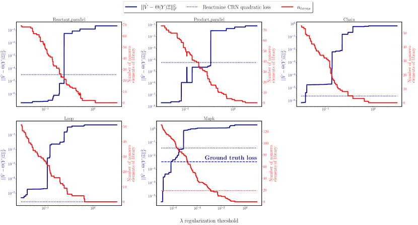
Figure S1: Quadratic training loss (blue) and number of nonzero terms in the library (red) found by SINDy as a function of $\lambda$ in our benchmark of reactant-parallel, product-parallel, chain, loop and MAPK CRNs. The dashed red line represents the actual number of nonzero terms in the ground truth ODE associated to each hidden CRN. The dashed darkblue line stands for the (non-zero due to numerical errors) quadratic loss value of the ground truth CRN.

Reactmine uses four hyperparameters which are optimized by grid search to minimize the quadratic loss criterion of Equation (7). For all the CRNs considered through the section, we search $\alpha\in[0.005,0.5],\beta\in\llbracket 4,8\rrbracket$ and $\gamma\in\llbracket 3,6\rrbracket$, except for the MAPK example where we search for $\alpha\in[0.0025,0.2],\beta\in\{6,8,10\}$ and $\gamma\in\llbracket 7,10\rrbracket$. We do not search for an optimal $\delta_{\max}$ and set its value to $3$ as a later shown sensibility analysis will demonstrate that this hyperparameter is quite unsensible. SINDy uses one hyperparameter, the sparsity-enforcing penalty coefficient $\lambda$. It turns out that in all the examples below, there is no value of $\lambda$ leading to both a good fit and a sparse model. In particular, there is no value of $\lambda$ for which the hidden dynamics are recovered, as illustrated by Fig. S1. For the sake of comparison to SINDy, we thus report the ODE system obtained using the (greatest) value of $\lambda$ that gives the same quadratic loss as Reactmine.

On the chain CRN example, Table 1 shows that Reactmine succeeds in recovering the hidden CRN by inferring $D\xrightarrow{1}E$ first, with the end of the trace as support, (Fig. 1c). Then the other reactions are learned in backward order, after successive derivative matrix updates, for subtracting the effects of each learned reaction. More details are given in Table S1 where we see that, in this example, the reactions are immediately inferred with the right kinetics and not changed by global re-optimization. Table S2 gives the hyperparameter settings used for the results reported in this section, the number of CRN candidates computed using the best hyperparameter setting found (here 128 chain CRN candidates) the learning time (here 0.31 seconds) and the hyperparameter grid search computation time (here 50 minutes).

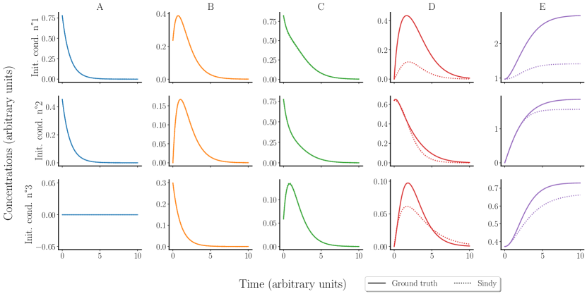
Figure S2: Simulation of the ODE model learned by SINDy in the Chain example using different initial conditions (doted line) compared with ground truth (solid line), showing erroneous dynamics for $D$ and $E$.

In this example, SINDy correctly infers the (ODE terms of the) hidden reaction $A\xrightarrow{1}B$, then a part of reaction $B\xrightarrow{1}C$ is present: $\dot{B}$ includes the term $-1.00B$, but only $0.18B$ can be found in $\dot{C}$ among several other terms that do not correspond to reactions. Likewise, the production of $E$ by the reaction $D\xrightarrow{1}E$ is correctly inferred, but the ODE associated with $D$ is $-0.37DE$ instead of $-1.00D$. Moreover, the learned ODEs are not able to generalize the dynamics of species $D$ and $E$ on traces that were not used during training (Fig. S2). It is worth noting in this respect that the chain CRN is composed of 8 ODE terms, whereas the SINDy library comprises $5\times(1+\frac{5\times 6}{2})=80$ terms in this example.

The second example concerns the MAPK signaling network, a ubiquitous CRN structure that is present in all eukaryote cells and in several copies. We consider the simplified two-stage (instead of three) CRN model composed of $7$ species and $7$ reactions of Qiao et al. (2007). The input species $A$ goes through a first stage of complexation and phosphorylation to produce the phosphorylated form $Ap$ which plays the role of a kinase on $B$ at the second stage to produce the doubly phosphorylated output species $Bpp$. Signal amplification is caused by the difference of concentrations by several orders of magnitude between the input and the output, (Fig. S3). For this example, we set trace parameters $T=100$ and $\Delta t=\frac{1}{3}$.

As shown in Table 1, Reactmine recovers $6$ out of $7$ reactions of the hidden CRN and $3$ other reactions: $ApB\xrightarrow{499.96}Bpp+Ap$, $B+Ap\xrightarrow{500.01}Ap$ and $Ap+B\xrightarrow{500.19}ApB+B$. It is worth remarking that by summing the ODE terms of the latter two reactions, we get the same effect as the already inferred reaction $Ap+B\xrightarrow{500}ApB$, but with the original rate constant value $1000$ by summing the two copies of the reaction. On the other hand, a variant of the missing reaction $ApBp\xrightarrow{150}Ap+Bpp$ is inferred by Reactmine, namely $Ap+Bp\xrightarrow{500}Ap+Bpp$, where the reactant complex, $ApBp$ replaced by its two components. Fig. S4 shows that this is a very good approximation of the ground truth dynamics, on the training trace, as well as on the other simulation traces obtained from different initial conditions.

On the other hand, the ODE system inferred by SINDy has no term close to the hidden CRN, contains two zero-valued differential functions for yet evolving species, and fails on sparsity with an average number of $15$ terms per non-zero ODE. A more detailed analysis presented in the lower right figure from Table 1 shows that SINDy is unable to produce sparse solutions displaying low error for any value of $\lambda$. In particular, the ODE systems associated with similar loss values as that of the CRN found by Reactmine involves 90 terms. It is worth remarking in that Figure that the loss of the ground truth CRN is not zero for the subtle reason that the loss is computed by an estimation of the derivative matrix by finite differences on a trace, produced by numerical integration with a more elaborate implicit method, and overfitted by SINDy for low values of $\lambda$. It is worth noting that the 7 ODEs of the MAPK CRN comprise a total of $20$ terms, whereas the SINDy library comprises $7\times(1+\frac{7\times 8}{2})=203$ terms. Likewise, for the chain CRN, this creates challenging sparse regression problems in the absence of strong independence properties between predictors (Zhao and Yu, 2006). The better results reported in (Mangan et al., 2016) may be explained by the recourse to multiple traces with different zeroes in the initial conditions, similarly to what has been shown in the context of Boolean models in (Carcano et al., 2017).

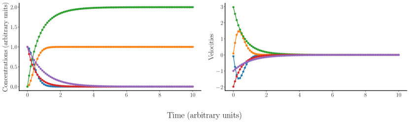
Figure S5: Learning trace and estimated derivatives for the Reactant-Parallel CRN.

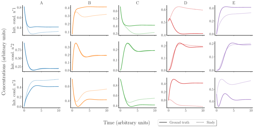
Figure S9: Simulation of the ODE model learned by SINDy in the Loop example using different initial conditions (doted line) compared with ground truth (solid line), showing erroneous dynamics on all species.

Table S1 summarizes the results obtained by Reactmine and SINDy on a benchmark of even smaller size CRNs presenting different kinds of difficulties. The learning traces used in those examples, also including the chain CRN, are detailed in Figs. S5–S8, together with their estimated velocities. The loop CRN adds a feedback reaction $E\xrightarrow{1}A$ to the chain CRN, leading to the stabilization of all molecular species on some common concentration value. Reactmine succeeds in recovering the hidden reactions in forward order, directly with the right kinetics. Here again, SINDy recovers some terms of the two first reactions and of the last reaction, but among many other overfitting terms which do not generalize to simulation traces obtained from different initial states,(Fig. S9).

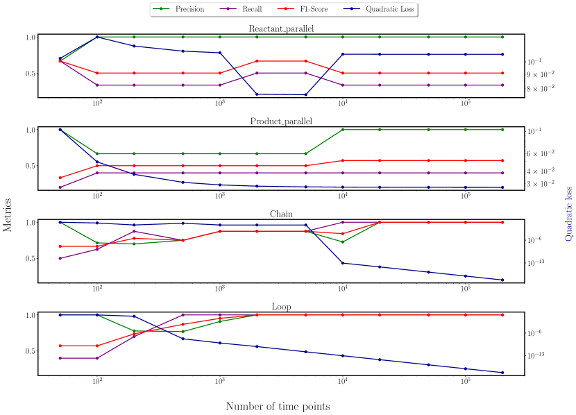
Figure S10: Sensitivity of SINDy to the number of time points with $\lambda$ selected to yield the highest binary $F_{1}$-Score (i.e. $F_{1}$-score with labels 1 for terms with non-zero coefficient in the ODEs, independently of their sign, and labels 0 for zero coefficient). Precision, recall, F1-score and quadratic loss are displayed as a function of the number of time points in the learning simulation trace used. With very high number of time points, SINDy succeeds in recovering the hidden chain and loop CRNs, but this is not the case for the reactant-parallel and product-parallel CRNs.

The reactant-parallel CRN is just composed of one catalytic reaction, $A+C\xrightarrow{1}B+C$, where the catalyst $C$ is produced by two concurrent reactions $D\xrightarrow{2}C$ and $E\xrightarrow{1}C$. Reactmine first infers the preponderant production of $C$ by $D$, then by $E$, after what the reaction catalyzed by $C$ is correctly inferred. One can notice that the rate constant first inferred for the reaction $E\xrightarrow{}C$ has a small value below its final value by two orders of magnitude. The reason is that right after the inference of $D\xrightarrow{}C$, reaction $E\xrightarrow{1.00}\emptyset$ is inferred prior to $E\xrightarrow{0.01}C$. The global re-optimization of rate constants has for effect in this case to set to $0$ the rate constant of the second reaction, in favor of the third reaction $E\xrightarrow{1}C$ which is thus finally recovered with the right kinetics. In this example, SINDy infers a wrong ODE system that does not reproduce the learning trace, even by increasing the number of time points (Fig. S10).

The product-parallel CRN is the symmetrical case of two concurrent consumptions of the catalyst $C$ with the production of species $D$ and $E$, on which SINDy similarly fails. Reactmine first infers the preponderant transformation of $C$ in $E$, then of $C$ in $D$ and then the correct catalyzed reaction with little correction of the rate constants by the global optimization phase, (Table S1).

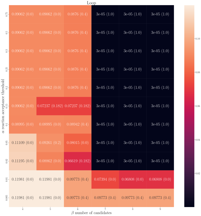
Figure 2: Sensitivity of Reactmine to $\alpha$ and $\beta$ hyperparameters for the loop CRN. Quadratic loss $\lVert{\bf{V}}-{\bf{F}}({\bf{Y}},{\bf{k}})\textbf{S}\rVert_{F}^{2}$ (lower, colored in black, is better) and F1-score (in parenthesis, higher is better). The colorbar levels relate to the quadratic loss. $\delta_{\text{max}}=3$ and $\gamma=6$.

3.2 Hyperparameter sensitivity analyses

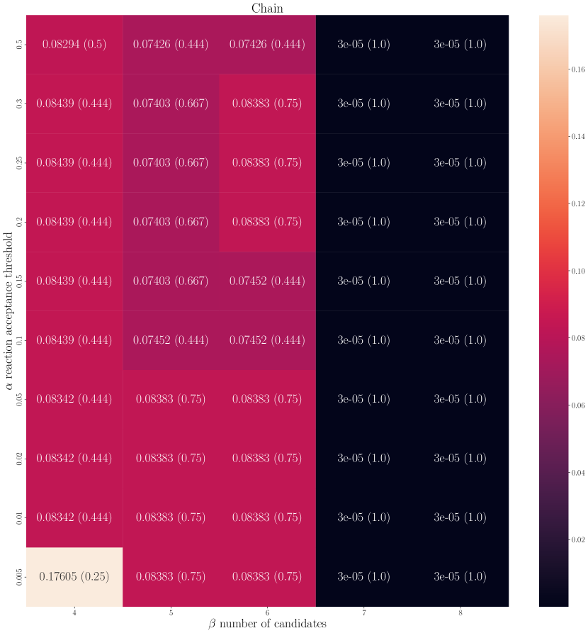
(a) Chain CRN

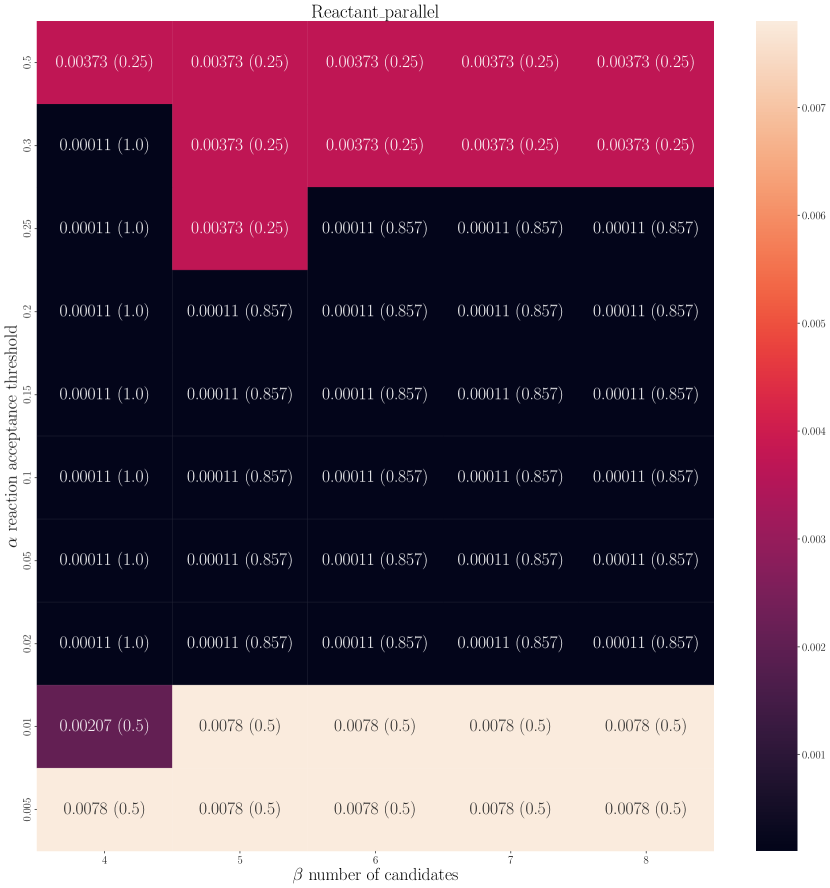
(b) Reactant Parallel CRN

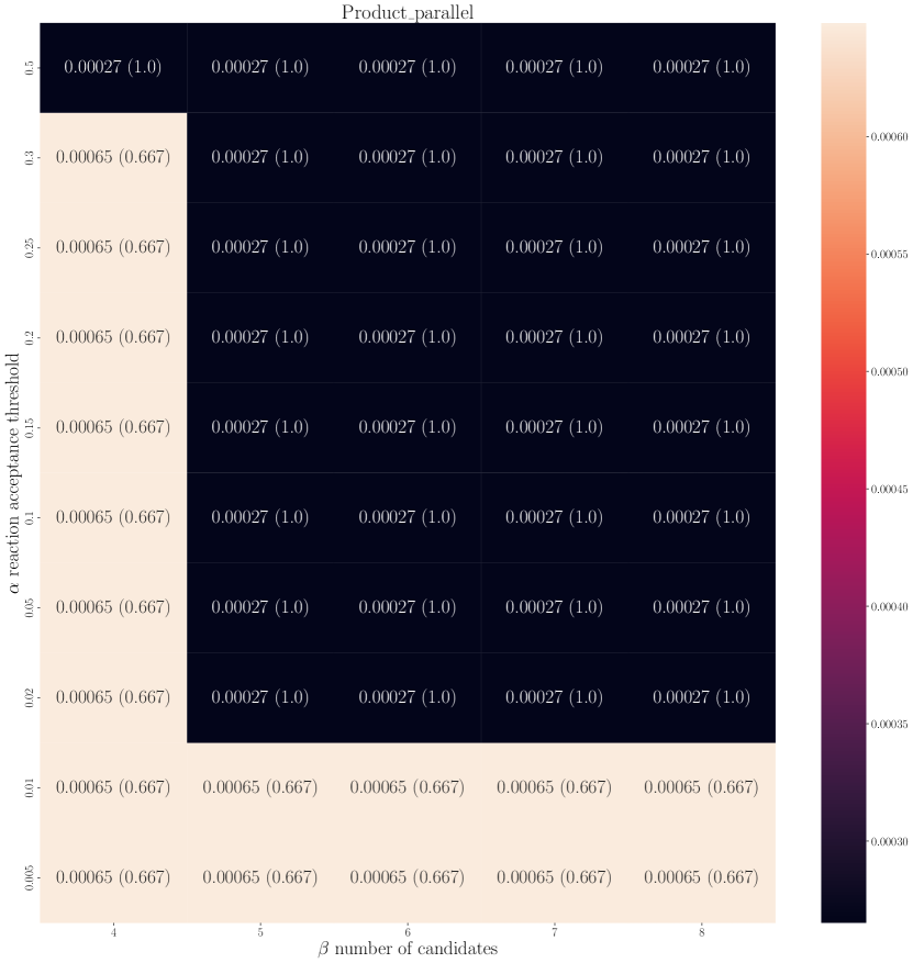
(c) Product Parallel CRN

Figure S11: Sensitivity of Reactmine to $\alpha$ and $\beta$ hyperparameters. Quadratic loss $\lVert{\bf{V}}-{\bf{F}}({\bf{Y}},{\bf{k}})\textbf{S}\rVert_{F}^{2}$ (lower is better) and F1-score (in parenthesis, higher is better). The colorbar levels relate to the quadratic loss. $\delta_{\text{max}}=3$ and $\gamma=6$ except for the reactant-parallel CRN where $\gamma=5$, as it yielded a better result.

In this section, we study the impact on the previous resuls of the hyperparameter values of Reactmine and of the number of time points. Reactine results are sensitive to both $\alpha$ and $\beta$ (Fig. 2 for the loop CRN, Fig. S11 for the other toy CRNs). In particular, there exist a region for which sufficiently many candidates are proposed and accepted (for the loop CRN, $\beta>6,\alpha>0.01$). Next, Fig. S12 also assesses the sensitivity with respect to $\gamma$ the maximal CRN size and $\delta_{\text{max}}$ the maximum absolute fold change between species variations in a reaction. Only the value of either $\delta_{\text{max}}$ or $\gamma$ is changed, the other hyperparameters are set to values leading to maximum $F_{1}$-score. $\gamma$ is a sensitive hyperparameter either in terms of quadratic loss value or $F_{1}$-score. This is expected as being the maximum CRN size, $\gamma$ has high impact on the flexibility of the network. One should remark that the $\gamma$ value associated with a perfect $F_{1}$-score is sometimes higher than the size of the hidden CRN. As previously mentioned in Section 3.1 for the case of the Reactant-Parallel CRN, this is due to the inference of reactions whose effect is later set to 0 upon global re-optimization. For this example, these steps were somewhat needed otherwise the ground truth CRN would have been recovered with $\gamma=3$. It is worth noticing that for all examples, the hyperparameter sets yielding the lowest quadratic loss are associated with highest F1-score for all CRNs, thus providing empirical evidence concerning the relevance of hyperparameter selection based on quadratic loss minimization.

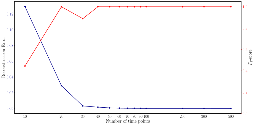
Figure S13: Sensitivity of Reactmine to the number of time points for the chain CRN with $\delta_{\text{max}}=3,\alpha=0.2,\beta=7,\gamma=5$. The time horizon of the simulation is $T=10$. The quadratic loss is reported in darkblue, the $F_{1}$-score in red. The x-axis is in log scale.

Now, the sensitivity to the number of time points in the trace is evaluated in Fig. S13 on the chain CRN. We observe an almost monotonic transition to high F1-score / low reconstruction error as the number of time points increases with optimal performance being reached above 40 time points only.

On the other hand, Fig. S10 shows that the failure of SINDy to recover the hidden CRNs persists independently of the number of time points for both the reactant and product-parallel examples. For these examples, increasing up to $2\times 10^{5}$ time points did not lead to perfect inference as can be seen from the $F_{1}$-score being different from $1$. The learned models display high precision but low recall, suggesting sparse but yet incomplete dynamics. However, the chain and loop CRN could be recovered using $10000$ and $500$ time points, respectively. This suggests that the problem of sparse regression in that approach rather comes from the high level of correlations observed in single CRN traces without the possibility to vary the zeroes in the initial conditions.

3.3 Evaluation on videomicroscopy data

Next, we apply Reactmine to time lapse videomicroscopy data in NIH-3T3 embryonic mouse fibroblasts (Feillet et al., 2014), used to develop a coupled model of the cell cycle and the circadian clock for this cell line (Traynard et al., 2016). The cell line was modified to include three fluorescent markers of the circadian clock and the cell cycle: the RevErb-$\alpha$::Venus clock gene reporter (Nagoshi et al., 2004) for measuring the expression of the circadian protein RevErb$\alpha$, and the Fluorescence Ubiquitination Cell Cycle Indicators (FUCCI), Cdt1 and Geminin, two cell cycle proteins which accumulate during the G1 and S/G2/M phases respectively, for measuring the cell cycle phases (Sakaue-Sawano et al., 2008). The cells were left to proliferate in vitro in standard culture medium supplemented with 20% of Fetal Bovine Serum. Fluorescence recording was performed in constant conditions with one image taken every 15 to 30 minutes during 72 hours.

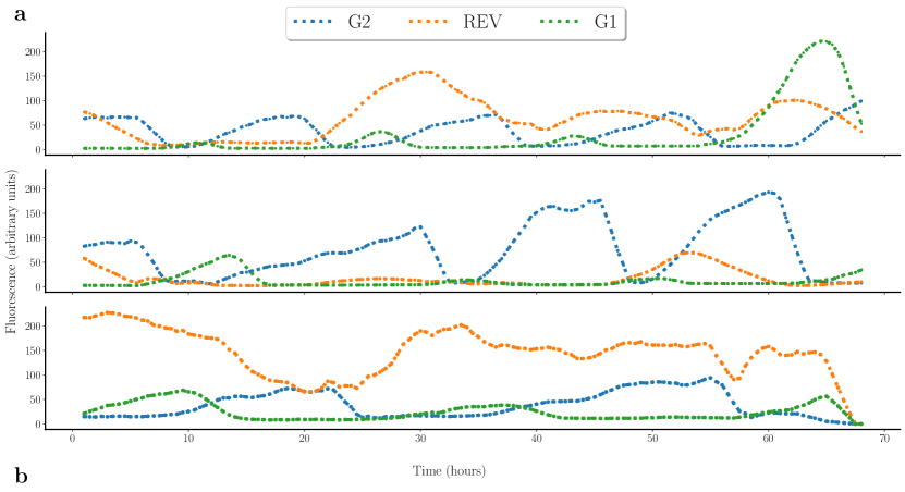
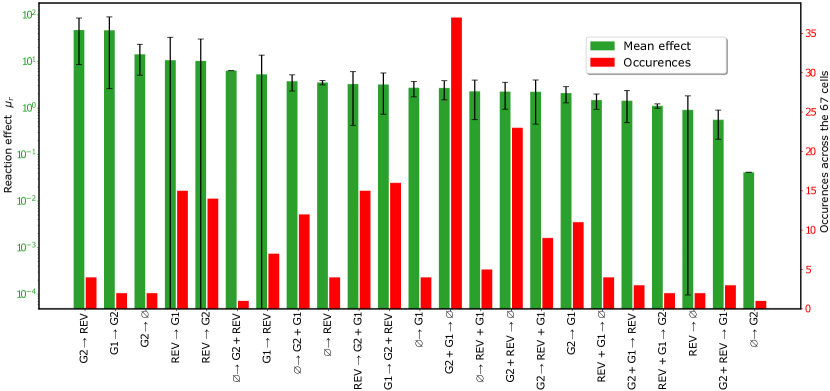
Figure 3: Results of Reactmine on fluorescence videomicroscopy dataset. a Plot of 3 cells among the 67 cells of the videomicroscopy data. Traces have been smoothed with a moving average. b Ranking of mean effect (green) and occurences (red) of inferred reactions on 67 cells. Bars in green report the mean effect of each reaction across time and cells in the videomicroscopy data. Standard deviation is computed across the cells.

A dataset of $67$ tracked cells was built from these experiments (Feillet et al., 2014), giving rise to fluorescence levels trajectories with high inter-cell variability and noise (Fig. 3a). Thus, our learning protocol will

• first smooth the curves with a sliding window of 2.5 h;

• apply Reactmine to infer a CRN for each cell individually, using Michaelis-Menten rate functions (as described in Section 2.3.2) in order to fit indirect effects, $\gamma=3$ in order to discover the main influences between the 3 variables, and the remaining three hyperparameters selected by grid search as mentioned in Section 2.3.5;

• then compute statistics on the number of reaction occurrences across the $C=67$ inferred CRNs (one per cell). Let $y_{i}^{(c)}$ be the fluorescence vector at time $t_{i}$ for cell $c$. We define the mean effect $\mu$ of a reaction $r=(R,P,f)$ on the derivative matrix as:

  $$\mu_{r}=\frac{1}{nC}\sum_{c=1}^{C}\sum_{i=1}^{n}f(y_{i}^{(c)})$$ (12)

Two reactions clearly stand out compared to the others in terms of effect (Fig. 3b). The first one , $G2\xrightarrow{}REV$, represents a possible effect of the cell cycle on the circadian clock through the activation of Rev-Erb$\alpha$ during the G2 phase, in agreement with the main surprising findings of the modeling study of (Traynard et al., 2016), using the same dataset. The second most impactful reaction effect-wise is $G1\xrightarrow{}G2$, the reaction accounting for the cell phase transition from G1 into S/G2/M. The reverse formal reaction $G1\xrightarrow{}G2$ which could perhaps be expected, is learned but ranked effect-wise behind several meaningless reactions. In terms of occurrence number, one can observe the predominance of a meaningless reaction $G2+G1\xrightarrow{}\emptyset$, present in 37 out of 67 cells, yet never inferred first, and with low rate constants.

3.4 Detection of systemic controls on clock gene transcription

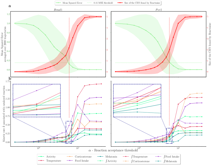
Figure 4: Inference of systemic drivers for Bmal1 and Per2 clock genes transcription by Reactmine. a Average and std for the mean square error (green) and number of reactions (red) for the CRNs inferred by Reactmine, as a function of $\alpha$ the reaction acceptance threshold. The statistics are computed over the $N=2000$ trajectories $\{y^{(j)}\}_{1\leq j\leq N}$ considered. The green dotted horizontal line represents a MSE threshold of 0.15, equivalent here to 15% of the variance left unexplained by the inferred CRN. The red dotted vertical line reveals that for both Bmal1 and Per2, CRNs with only two reactions are enough to reach a MSE below 0.15. b Mean rate constant associated to a catalyzed reaction reported as a function of $\alpha$. The mean is computed over the $N=2000$ trajectories $\{y^{(j)}\}_{1\leq j\leq N}$. The plot zoom corresponds to $\alpha\approx 6$, equivalent to an average number of two reactions per CRN.

In this section, we apply Reactmine to biological data measuring the circadian rhythms of five systemic regulators in mice: body temperature, rest-activity rhythms, food intake, plasma corticosterone and melatonin, as well as the circadian mRNA expression data in the mouse liver of two core clock genes: Bmal1 and Per2. These datasets have been analyzed in (Martinelli et al., 2021) to infer the preponderant systemic regulators on clock gene transcription through another model learning approach. Using an ODE-based model of the liver circadian clock (Hesse et al., 2021) as well as data from four mouse classes, transcription activation profiles $y$ were derived for each gene. These profiles were regressed on systemic regulators with the aim to infer the significant drivers of clock gene transcription. Let us now use Reactmine for this task and compare the results.

Since we are looking for an influence model rather than a reaction model properly speaking, we shall use the classical encoding of an influence by one formal reaction catalyzed by the source of the influence (Fages et al., 2018). We will thus enforce in Reactmine the search of influence reactions of the form $z\xrightarrow{k}z+y$ where $z$ is one systemic regulator, $y$ one transcription activation profile for a target gene. We shall assume mass action law kinetics representing influence forces.

Furthermore, it is assumed that a systemic regulator $z$ acts either directly, or indirectly though intermediate species by considering its integral counterpart $\int z$, but not both ways. The 5 systemic regulators thus lead to 10 possible influences on Bmal1 and Per2 genes. Reactmine hyperparameters $\gamma$ and $\beta$ can be set accordingly to 5 and 10. $\delta_{\max}=3$ as in previous experiments. Only $\alpha$, the influence acceptance threshold, needs to be searched in order to restrict ourselves to preponderant influences only. Fig. 4a shows the mean quadratic loss and number of influences of the CRNs inferred by Reactmine for different values of $\alpha$. For $\alpha=6$, the inferred CRNs with only two influences in average reach an MSE below 0.15 - or equivalently - explain more than $85\%$ of the variance.

Figure 4b recapitulates the mean kinetic rate constants of the inferred reactions obtained across the traces as a function of $\alpha$, with the zoom part corresponding to $\alpha=6$, for which the inferred CRNs contain 2 reactions in average. Remarkably, Reactmine discovers that Food Intake and Temperature are the main influencing factors of clock gene transcription, either in a direct or an indirect manner. Using $\alpha=6$, for Bmal1, the indirect action of Food Intake is deemed the most relevant regulator, followed by the indirect action of Temperature and the direct action of Corticosterone, in agreement with Martinelli et al. (2021). Concerning Per2, Food Intake and Temperature again stand out as most important systemic drivers. The recovered regulation importance ordering is the same as in (Martinelli et al., 2021) (Fig. 6B-C), except for one permutation between $\int$Corticosterone and $\int$Temperature.

4 Conclusion

Reactmine is an algorithm specially designed to infer biochemical reactions with kinetics, between molecular species observed in wild type time series data, i.e. without gene knock out nor other possibilities to put initial conditions to $0$ at will. On a benchmark of hidden CRNs of increasing difficulty, including one model of MAPK signal transduction levels (Qiao et al., 2007), we have shown that Reactmine is able to recover the hidden CRN, or an essentially equivalent form of it, from one single ODE simulation trace. On the opposite, the state-of-the-art sparse regression algorithm for non linear dynamical systems, SINDy Brunton et al. (2016), with appropriate function libraries for the examples, fails to infer sparse ODE systems in that setting, and even to reproduce the simulation traces obtained from different initial states.

The behavior of sparse regression algorithms is indeed conditional to assumptions about the low level of correlation between predictors (Zhao and Yu, 2006). Those hypotheses are not satisfied in the context of wild type time series data, specifically in a low data regime. The possibility of varying the traces by setting to 0 some initial conditions has a de-correlation effect which may explain the better results reported in Mangan et al. (2016), similarly to what has been shown for boolean models in Carcano et al. (2017). Those arguments are the subject of current work in the general context of sparse identification of non linear dynamics.

Reactmine solves those issues by not relying on sparse regression but on a statistical search algorithm with a bounded depth of reaction candidates which ensures sparsity by construction. Reactmine uses four hyperparameters. In all our examples, the maximum ratio $\delta_{\max}$ of variation between reactants and products for the inference of one reaction skeleton at a transition could be fixed to 3. On the other hand, sensitivity analysis shows that the other three hyperparameters are important and are currently determined by gridsearch in absence of better understanding of their sensitivty to the dimension and other characteristics of the time series data. When applied to real biological data of videomicroscopy data and systemic circadian controls of clock genes, we have shown that Reactmine is able to retrieve the main conclusions of the model-based analyses done respectively in Traynard et al. (2016) and Martinelli et al. (2021) on the same datasets.

These encouraging results should motivate applying Reactmine to new study cases on the one hand, possibly dropping the restriction of 0/1 stoichiometry for a limited number of reaction schemas, and on the other hand, generalizing Reactmine by introducing hidden variables in inconsistent transitions to deal with the further challenge of learning models with latent species.

Supplementary Material for Reactmine: a statistical search algorithm for inferring chemical reactions from time series data

S1 Extending Reactmine to Michaelis Menten and Hill Kinetics

Reactmine is also compatible with other forms of kinetics, provided that a measure of quality of reaction parameters can be computed, such as the coefficient of variation. A single-reactant reaction $(R,P,f)$ follows Michaelis Menten kinetics if $\forall j\in R\cup P,~{}\forall i\in\{1,\dots,n\}$

$$v_{i,j}=s_{j}f({\bf{Y}}_{i,\bullet})=s_{j}\nu_{\max}\frac{y_{i,u}}{y_{i,u}+K_{m}}$$ (13)

where $\nu_{\max}$ and $K_{m}$ are parameters, and $R=\{u\}$. Note that Michaelis Menten kinetics are not defined for bimolecular reactions.

As $y_{u}\to+\infty,~{}\lvert v_{j}\rvert\to\nu_{\max}$. Besides, $\lvert v_{j}\rvert$ being an increasing function of $y_{u}$, an estimator of $\nu_{\max}$ can be obtained as the highest observed derivative $\lvert v_{i,j}\rvert$ on the whole transitions: for all $j\in R\cup P$

$$\tilde{\nu}_{\max,j}=\underset{i\in\{1,\dots,n\}}{\max}\lvert v_{i,j}\rvert$$ (14)

Then, $K_{m}$ is defined as the value of reactant concentration for which the associated derivative is equal to $\frac{\nu_{\max}}{2}$. Since measurements are only available at discrete time points, one has

$$\hat{K}_{m,j}=y_{i^{*},u}\quad\text{ with }i^{*}=\underset{i\in\{1,\dots,n\}}{\operatorname*{argmin}}~{}\left\lvert\lvert v_{i,j}\rvert-\frac{\tilde{\nu}_{\max,j}}{2}\right\rvert$$ (15)

Once an estimator for $K_{m}$ has been provided, we apply the same principle as in Equation 4 from the main text, to obtain a new estimator of $\nu_{\max}~{}\forall j\in R\cup P$

$$\hat{\nu}_{\max,j}=\frac{s_{j}}{\#\mathcal{T}(r)}\sum_{i\in\mathcal{T}(r)}v_{i,j}\frac{\hat{K}_{m,j}+y_{i,u}}{y_{i,u}}$$ (16)

The computation described above also applies to Hill Kinetics of order $\eta$, $\forall j\in R\cup P,~{}\forall i\in\{1,\dots,n\}$

$$v_{i,j}=s_{j}f({\bf{Y}}_{i,\bullet})=s_{j}\nu_{\max}\frac{y_{i,u}^{\eta}}{y_{i,u}^{\eta}+K_{m}}$$ (17)

However, for Michaelis-Menten and Hill kinetics, the optimization of $\hat{K}_{m}$ constants leads to a non-convex problem with no convergence guarantees.

S2 Detailed results of Reactmine and SINDy

Computation times reported here have been obtained on a Macbook M1 2020 13" with 8 cores. For Reactmine, the grid search was parallelized. For SINDy (Brunton et al., 2016) we used the pysindy library with STLSQ (sequential least square thresholding) optimizer, as we observed that it yielded better results than Lasso or SR3. We chose to report in Table S1 and in the main text, the ODE system inferred by SINDy with a value of regularization hyperparameter $\lambda$ that leads to the quadratic loss (which is not zero due to numerical integration errors) of the ground truth CRN recovered by Reactmine.

Name	Hidden CRN	CRN inferred by Reactmine	ODE system inferred by SINDy
Chain	$\textbf{A}\xrightarrow{1}B$ $B\xrightarrow{1}C$ $C\xrightarrow{1}D$ $D\xrightarrow{1}E$	${\color[rgb]{0.0,0.5,0.0}D\xrightarrow[1.00041]{0.99869}E}$ ${\color[rgb]{0.0,0.5,0.0}C\xrightarrow[1.00071]{0.99836}D}$ ${\color[rgb]{0.0,0.5,0.0}B\xrightarrow[0.99753]{1.00102}C}$ ${\color[rgb]{0.0,0.5,0.0}A\xrightarrow[1.00107]{1.00069}B}$	$\left\{\begin{array}[]{l}\begin{aligned} \dot{A}&={\color[rgb]{0.0,0.5,0.0}-1.00A}\\[-7.0pt] \dot{B}&={\color[rgb]{0.0,0.5,0.0}1.00A-1.00B}\\[-7.0pt] \dot{C}&={\color[rgb]{0.0,0.5,0.0}1.03B-1.03C}~{}{\color[rgb]{1,0,0}+0.01D-0.06AB}\\[-7.0pt] \dot{D}&={\color[rgb]{1,0,0}0.33B-0.64DE}\\[-7.0pt] \dot{E}&={\color[rgb]{0.0,0.5,0.0}1.00D}\end{aligned}\end{array}\right.$
Loop	$\textbf{A}\xrightarrow{1}B$ $B\xrightarrow{1}C$ $C\xrightarrow{1}D$ $D\xrightarrow{1}E$ $E\xrightarrow{1}\textbf{A}$	${\color[rgb]{0.0,0.5,0.0}A\xrightarrow[1.00005]{0.99958}B}$ ${\color[rgb]{0.0,0.5,0.0}B\xrightarrow[0.99243]{0.99748}C}$ ${\color[rgb]{0.0,0.5,0.0}C\xrightarrow[0.99156]{0.99772}D}$ ${\color[rgb]{0.0,0.5,0.0}D\xrightarrow[0.92045]{0.99771}E}$ ${\color[rgb]{0.0,0.5,0.0}E\xrightarrow[1.00007]{0.99758}A}$	$\left\{\begin{array}[]{l}\begin{aligned} \dot{A}&={\color[rgb]{0.0,0.5,0.0}-1.00A+1.03E}~{}{\color[rgb]{1,0,0}-0.006D-0.07AE-0.06DE}\\[-7.0pt] \dot{B}&={\color[rgb]{0.0,0.5,0.0}1.00A-1.00B}~{}{\color[rgb]{1,0,0}+0.004C+0.001AB-0.211AC-0.092BC}\\[-7.0pt] \dot{C}&={\color[rgb]{0.0,0.5,0.0}1.14B-1.18C}~{}{\color[rgb]{1,0,0}-0.002D-0.17AB+0.39CD}\\[-7.0pt] \dot{D}&={\color[rgb]{1,0,0}0.35B-0.35E}\\[-7.0pt] \dot{E}&={\color[rgb]{1,0,0}0.39C+0.457E-4.21AE}\end{aligned}\end{array}\right.$
Reactant Parallel	$\textbf{A}+C\xrightarrow{3}B+C$ $\textbf{D}\xrightarrow{2}C$ $\textbf{E}\xrightarrow{1}C$	${\color[rgb]{0.0,0.5,0.0}D\xrightarrow[1.97698]{2.00109}C}$ ${\color[rgb]{0.0,0.5,0.0}E\xrightarrow[0.00526]{1.00101}C}$ ${\color[rgb]{0.0,0.5,0.0}A+C\xrightarrow[2.95790]{2.94380}B+C}$	$\left\{\begin{array}[]{l}\begin{aligned} \dot{A}&={\color[rgb]{1,0,0}-1.12A-510000276790.32C-0.87AB+1.03AD}\\[-7.0pt] &\quad+{\color[rgb]{0.0,0.5,0.0}510000276788.57AC}~{}{\color[rgb]{1,0,0}+510000276790.32BC-0.04DC}\\[-5.0pt] \dot{B}&={\color[rgb]{1,0,0}1.12A+510000276790.24C+0.87AB-1.04AD}\\[-7.0pt] &\quad{\color[rgb]{0.0,0.5,0.0}-510000276788.49AC}~{}{\color[rgb]{1,0,0}-510000276790.24BC+0.04DC}\\[-5.0pt] \dot{C}&={\color[rgb]{0.0,0.5,0.0}-2.20D}~{}{\color[rgb]{1,0,0}+0.02E-0.19AD+0.40DE}\\[-7.0pt] \dot{D}&={\color[rgb]{1,0,0}0.07A}~{}{\color[rgb]{0.0,0.5,0.0}+1.96D+1.02E}~{}{\color[rgb]{1,0,0}-0.06DE}\\[-7.0pt] \dot{E}&={\color[rgb]{0.0,0.5,0.0}-1.00E}\end{aligned}\end{array}\right.$
Product Parallel	$\textbf{A}+\textbf{C}\xrightarrow{1}B+\textbf{C}$ $\textbf{C}\xrightarrow{2}D$ $\textbf{C}\xrightarrow{3}E$	${\color[rgb]{0.0,0.5,0.0}C\xrightarrow[3.12657]{2.93602}E}$ ${\color[rgb]{0.0,0.5,0.0}C\xrightarrow[2.08438]{1.95735}D}$ ${\color[rgb]{0.0,0.5,0.0}A+C\xrightarrow[1.04002]{0.96372}B+C}$	$\left\{\begin{array}[]{l}\begin{aligned} \dot{A}&={\color[rgb]{1,0,0}-0.93C}\\[-7.0pt] \dot{B}&={\color[rgb]{1,0,0}0.93C}\\[-7.0pt] \dot{C}&={\color[rgb]{1,0,0}68364.34-84189.93A+32887.73C+14190.64D}\\[-7.0pt] &\quad{\color[rgb]{1,0,0}+21285.97E-17066.849AC-40273.85AE+990.87CD}\\[-7.0pt] &\quad{\color[rgb]{1,0,0}+990.83CD+1486.24CE+7919.89DE}\\[-5.0pt] \dot{D}&={\color[rgb]{0.0,0.5,0.0}3.73C}~{}{\color[rgb]{1,0,0}-1.84AC}\\[-7.0pt] \dot{E}&={\color[rgb]{1,0,0}65012.55A-60751.24C-77885.60E-4258.48AC}\\[-7.0pt] &\quad{\color[rgb]{1,0,0}-10214.65CE-27068.38DE}\end{aligned}\end{array}\right.$
MAPK	$\textbf{A}\xrightarrow{0.0045}Ap$ $Ap+\textbf{B}\xrightarrow{1000}ApB$ $ApB\xrightarrow{150}Ap+\textbf{B}$ $ApB\xrightarrow{150}Ap+Bp$ $Ap+Bp\xrightarrow{1000}ApBp$ $ApBp\xrightarrow{150}Ap+Bp$ $ApBp\xrightarrow{150}Ap+Bpp$	${\color[rgb]{0.0,0.5,0.0}A\xrightarrow[0.0045]{0.00449}Ap}$ ${\color[rgb]{1,0,0}Bp+Ap\xrightarrow[499.96702]{499.96702}Bpp+Ap}$ ${\color[rgb]{1,.5,0}B+Ap\xrightarrow[500.01476]{500.01476}Ap}$ ${\color[rgb]{0.0,0.5,0.0}ApB\xrightarrow[150.03923]{150.04220}Ap+Bp}$ ${\color[rgb]{0.0,0.5,0.0}Ap+B\xrightarrow[501.19119]{501.19113}ApB}$ ${\color[rgb]{0.0,0.5,0.0}ApB\xrightarrow[150.36767]{150.37064}Ap+B}$ ${\color[rgb]{0.0,0.5,0.0}Ap+Bp\xrightarrow[517.78581]{517.78303}ApBp}$ ${\color[rgb]{0.0,0.5,0.0}ApBp\xrightarrow[155.32578]{155.33508}Ap+Bp}$ ${\color[rgb]{1,.5,0}Ap+B\xrightarrow[500.18851]{500.18846}ApB+B}$	$\left\{\begin{array}[]{l}\begin{aligned} \dot{Bpp}&={\color[rgb]{1,0,0}11764.89-9818.81Bpp-21809.21Ap-64774.82ApBp-9881.63Bp}\\[-5.0pt] &\quad{\color[rgb]{1,0,0}+109653.06ApB-10102.57B-23028.83A+23087.90Bpp\times Ap}\\[-5.0pt] &\quad{\color[rgb]{1,0,0}+47383.24Bpp\times ApBp+0.01Bpp\times Bp-94598.54Bpp\times ApB}\\[-5.0pt] &\quad{\color[rgb]{1,0,0}+0.05Bpp\times B+24104.25Bpp\times A+58119.14Ap\times Bp}\\[-5.0pt] &\quad{\color[rgb]{1,0,0}+117674.08Ap\times B+68314.42ApBp\times Bp+239788.36ApBp\times B}\\[-5.0pt] &\quad{\color[rgb]{1,0,0}-171491.97Bp\times ApB+0.03Bp\times B+45027.82Bp\times A+118690.34B\times A}\\[-5.0pt] \dot{Ap}&={\color[rgb]{1,0,0}0.003Bp-0.001Bpp\times Bp-0.004Bpp\times B-0.002Bp\times B}\\[-5.0pt] \dot{ApBp}&={\color[rgb]{1,0,0}-0.002Bp+0.001Bpp\times Bp+0.004Bpp\times B+0.002Bp\times B}\\[-5.0pt] \dot{Bp}&={\color[rgb]{1,0,0}-11345.814+9469.53Bpp+20253.98Ap}~{}{\color[rgb]{0.0,0.5,0.0}+62939.32ApBp}\\[-5.0pt] &\quad{\color[rgb]{1,0,0}+9525.97Bp-105529.77ApB+9401.39B+22299.11A}\\[-5.0pt] &\quad{\color[rgb]{1,0,0}-21772.25Bpp\times Ap-45730.13Bpp\times ApBp-0.01Bpp\times Bp}\\[-5.0pt] &\quad{\color[rgb]{1,0,0}+91003.53Bpp\times ApB-0.05Bpp\times B-23476.51Bpp\times A}\\[-5.0pt] &\quad{\color[rgb]{0.0,0.5,0.0}-56249.34Ap\times Bp}~{}{\color[rgb]{1,0,0}+996.55Ap\times B-64537.43ApBp\times Bp}\\[-5.0pt] &\quad{\color[rgb]{1,0,0}-113908.83ApBp\times B+163092.38Bp\times ApB-0.03Bp\times B}\\[-5.0pt] &\quad{\color[rgb]{1,0,0}-42276.50Bp\times A+113704.11ApB\times B-763.549B\times A}\\[-5.0pt] \dot{ApB}&=0\\[-5.0pt] \dot{B}&={\color[rgb]{1,0,0}-668.78+557.83Bpp+1724.07Ap+2552.29ApBp}\\[-5.0pt] &\quad{\color[rgb]{1,0,0}+564.79Bp-5063.51ApB+551.20B+784.94A}\\[-5.0pt] &\quad{\color[rgb]{1,0,0}-1609.99Bpp\times Ap+-1960.37Bpp\times ApBp-0.001Bpp\times Bp}\\[-5.0pt] &\quad{\color[rgb]{1,0,0}+4399.19Bpp\times ApB-0.01Bpp\times B-827.38Bpp\times A}\\[-5.0pt] &\quad{\color[rgb]{1,0,0}-3441.84Ap\times Bp+543.68Ap\times B-4279.75ApBp\times Bp}\\[-5.0pt] &\quad{\color[rgb]{1,0,0}-8537.02ApBp\times B+10869.45Bp\times ApB}~{}{\color[rgb]{0.0,0.5,0.0}-0.003Bp\times B}\\[-5.0pt] &\quad{\color[rgb]{1,0,0}-3146.138Bp\times A+6610.523ApB\times B+1384.463B\times A}\\ \dot{A}&=0\end{aligned}\end{array}\right.$

Table S1: Results obtained by Reactmine and SINDy on hidden CRNs using a single simulation trace from one initial state containing the molecular species indicated in bold in the first column. The learned reactions are indicated in green if they belong to the hidden CRN, in yellow if they lead to equivalent terms of the associated ODEs, and in red otherwise. For a learned reaction, the number written underneath the arrow is the initial rate constant value learned with the reaction, before global re-optimization. For the ODE systems inferred by SINDy, the terms are coloured in green if they correspond to the kinetics of some hidden reactions, regardless of the precise kinetic constant value as long as the sign is exact, and in red otherwise.

CRN	Hyperparameters $(\alpha,\ \beta,\ \delta_{\max},~{}\gamma)$	Computation time in seconds	Number of inferred CRNs	Grid search values for $(\alpha,\ \beta,~{}\delta_{\max},\ \gamma)$	Computation time with grid search
Chain	(0.02, 7, 3, 4)	0.31	128	$\alpha\in\{0.005,0.01,0.02,0.05,0.1,0.15,0.2,0.25,0.3,0.5\}$ $\beta\in\{4,5,6,7,8\}$ $\delta_{\max}=3$ $\gamma\in\{3,4,5,6\}$	3035.95
Loop	(0.02, 7, 3, 6)	40.78	4198	$\alpha\in\{0.005,0.01,0.02,0.05,0.1,0.15,0.2,0.25,0.3,0.5\}$ $\beta\in\{4,5,6,7,8\}$ $\delta_{\max}=3$ $\gamma\in\{3,4,5,6\}$	30643.19
Reactant-Parallel	(0.02, 4, 3, 5)	1.81	265	$\alpha\in\{0.005,0.01,0.02,0.05,0.1,0.15,0.2,0.25,0.3,0.5\}$ $\beta\in\{4,5,6,7,8\}$ $\delta_{\max}=3$ $\gamma\in\{3,4,5,6\}$	970.23
Product-Parallel	(0.02, 5, 3, 3)	0.13	24	$\alpha\in\{0.005,0.01,0.02,0.05,0.1,0.15,0.2,0.25,0.3,0.5\}$ $\beta\in\{4,5,6,7,8\}$ $\delta_{\max}=3$ $\gamma\in\{3,4,5,6\}$	334.06
MAPK	(0.02, 7, 3, 10)	3012.85	33104	$\alpha\in\{0.0025,0.005,0.0075,0.01,0.015,0.02,0.025,0.03,0.04,0.05,0.1,0.2\}$ $\beta\in\{6,8,10\}$ $\delta_{\max}=3$ $\gamma\in\{7,8,9,10\}$	77179.92

Table S2: Reactmine computation times and hyperparameter values used for the results reported in Table S1. The best hyperparameter settings indicated in the second column for each example, are found by grid search with a range of values reported in the third column, and a computation time given in the last column. The CRN learning computation times in these settings are given in the third column, with the number of generated CRN candidates in the fourth column.

${\color[rgb]{0.8901960784313725,0.4666666666666667,0.7607843137254902}A}\xrightarrow{0.0045}{\color[rgb]{1.0,0.4980392156862745,0.054901960784313725}Ap}$
${\color[rgb]{1.0,0.4980392156862745,0.054901960784313725}Ap}+{\color[rgb]{0.5490196078431373,0.33725490196078434,0.29411764705882354}B}\xrightarrow{1000}{\color[rgb]{0.5803921568627451,0.403921568627451,0.7411764705882353}ApB}$
${\color[rgb]{0.5803921568627451,0.403921568627451,0.7411764705882353}ApB}\xrightarrow{150}{\color[rgb]{1.0,0.4980392156862745,0.054901960784313725}Ap}+{\color[rgb]{0.5490196078431373,0.33725490196078434,0.29411764705882354}B}$
${\color[rgb]{0.5803921568627451,0.403921568627451,0.7411764705882353}ApB}\xrightarrow{150}{\color[rgb]{1.0,0.4980392156862745,0.054901960784313725}Ap}+{\color[rgb]{0.8392156862745098,0.15294117647058825,0.1568627450980392}Bp}$
${\color[rgb]{1.0,0.4980392156862745,0.054901960784313725}Ap}+{\color[rgb]{0.8392156862745098,0.15294117647058825,0.1568627450980392}Bp}\xrightarrow{1000}{\color[rgb]{0.17254901960784313,0.6274509803921569,0.17254901960784313}ApBp}$
${\color[rgb]{0.17254901960784313,0.6274509803921569,0.17254901960784313}ApBp}\xrightarrow{150}{\color[rgb]{1.0,0.4980392156862745,0.054901960784313725}Ap}+{\color[rgb]{0.8392156862745098,0.15294117647058825,0.1568627450980392}Bp}$
${\color[rgb]{0.17254901960784313,0.6274509803921569,0.17254901960784313}ApBp}\xrightarrow{150}{\color[rgb]{1.0,0.4980392156862745,0.054901960784313725}Ap}+{\color[rgb]{0.12156862745098039,0.4666666666666667,0.7058823529411765}Bpp}$

Figure S3: Learning trace and estimated derivatives for the MAPK CRN. The lower panel shows the same plots with concentrations and derivatives normalized by their maximal values along the trace for visualization purposes.

Figure S4: Reproduction of the MAPK CRN simulation traces obtained from different initial conditions using the CRN inferred by Reactmine. Time-resolved species concentrations are normalized to their maximal value across the trace. $y_{0}^{(1)}=(2,0,0,0,0,0.5,0.01);y_{0}^{(2)}=(0,0,0,0,0,1,0.1);y_{0}^{(3)}=(0,0,0,0,0,1.5,0.001)$. The second column displays the loss between the simulation traces of the MAPK CRN and the CRN inferred by Reactmine.

${\color[rgb]{0.12156862745098039,0.4666666666666667,0.7058823529411765}A}+{\color[rgb]{0.17254901960784313,0.6274509803921569,0.17254901960784313}C}\xrightarrow{3}{\color[rgb]{1.0,0.4980392156862745,0.054901960784313725}B}+{\color[rgb]{0.17254901960784313,0.6274509803921569,0.17254901960784313}C}$
${\color[rgb]{0.8392156862745098,0.15294117647058825,0.1568627450980392}D}\xrightarrow{2}{\color[rgb]{0.17254901960784313,0.6274509803921569,0.17254901960784313}C}$
${\color[rgb]{0.5803921568627451,0.403921568627451,0.7411764705882353}E}\xrightarrow{1}{\color[rgb]{0.17254901960784313,0.6274509803921569,0.17254901960784313}C}$

${\color[rgb]{0.12156862745098039,0.4666666666666667,0.7058823529411765}A}+{\color[rgb]{0.17254901960784313,0.6274509803921569,0.17254901960784313}C}\xrightarrow{1}{\color[rgb]{1.0,0.4980392156862745,0.054901960784313725}B}+{\color[rgb]{0.17254901960784313,0.6274509803921569,0.17254901960784313}C}$
${\color[rgb]{0.17254901960784313,0.6274509803921569,0.17254901960784313}C}\xrightarrow{2}{\color[rgb]{0.8392156862745098,0.15294117647058825,0.1568627450980392}D}$
${\color[rgb]{0.17254901960784313,0.6274509803921569,0.17254901960784313}C}\xrightarrow{3}{\color[rgb]{0.5803921568627451,0.403921568627451,0.7411764705882353}E}$

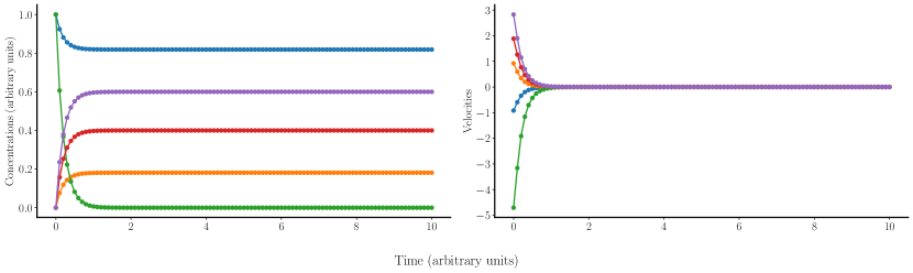
Figure S6: Learning trace and estimated derivatives for the Product-Parallel CRN.

${\color[rgb]{0.12156862745098039,0.4666666666666667,0.7058823529411765}A}\xrightarrow{1}{\color[rgb]{1.0,0.4980392156862745,0.054901960784313725}B}\xrightarrow{1}{\color[rgb]{0.17254901960784313,0.6274509803921569,0.17254901960784313}C}\xrightarrow{1}{\color[rgb]{0.8392156862745098,0.15294117647058825,0.1568627450980392}D}\xrightarrow{1}{\color[rgb]{0.5803921568627451,0.403921568627451,0.7411764705882353}E}$

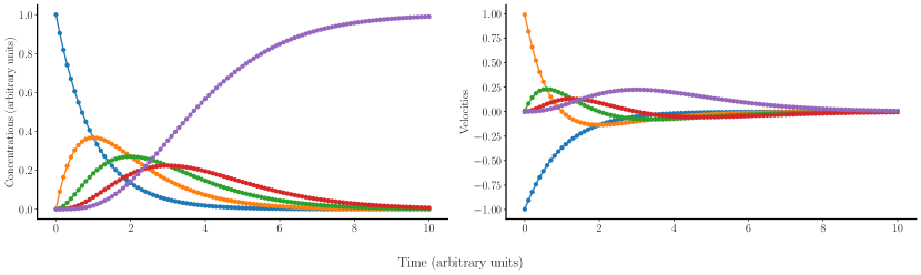
Figure S7: Learning trace and estimated derivatives for the Chain CRN.

${\color[rgb]{0.12156862745098039,0.4666666666666667,0.7058823529411765}A}\xrightarrow{1}{\color[rgb]{1.0,0.4980392156862745,0.054901960784313725}B}\xrightarrow{1}{\color[rgb]{0.17254901960784313,0.6274509803921569,0.17254901960784313}C}\xrightarrow{1}{\color[rgb]{0.8392156862745098,0.15294117647058825,0.1568627450980392}D}\xrightarrow{1}{\color[rgb]{0.5803921568627451,0.403921568627451,0.7411764705882353}E}\xrightarrow{1}{\color[rgb]{0.12156862745098039,0.4666666666666667,0.7058823529411765}A}$

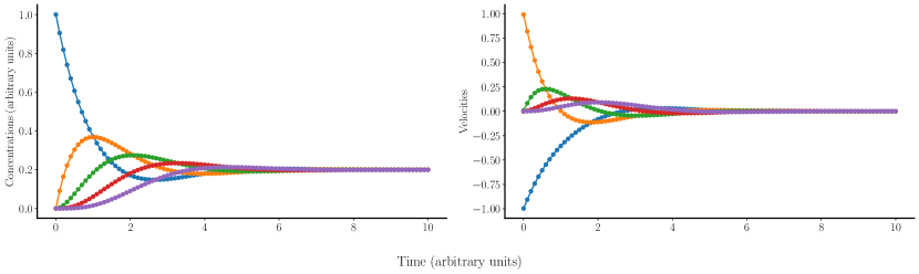
Figure S8: Learning trace and estimated derivatives for the Loop CRN.

Figure S12: Sensitivity of Reactmine to $\delta_{\max}$ and $\gamma$ hyperparameters. The quadratic loss is reported in darkblue, the $F_{1}$-score in red, negated for visualization purposes.

References

- Aalto et al. (2020) Aalto, A., Viitasaari, L., Ilmonen, P., Mombaerts, L., and Gonçalves, J. (2020). Gene regulatory network inference from sparsely sampled noisy data. Nature Communications, 11(1).
- Brunton et al. (2016) Brunton, S. L., Proctor, J. L., and Kutz, J. N. (2016). Discovering governing equations from data by sparse identification of nonlinear dynamical systems. Proceedings of the National Academy of Sciences, pages 3932–3937.
- Carcano et al. (2017) Carcano, A., Fages, F., and Soliman, S. (2017). Probably Approximately Correct Learning of Regulatory Networks from Time-Series Data. In CMSB’17: Proceedings of the fifteenth international conference on Computational Methods in Systems Biology, volume 10545, pages 74–90.
- Fages et al. (2018) Fages, F., Martinez, T., Rosenblueth, D., and Soliman, S. (2018). Influence networks compared with reaction networks: Semantics, expressivity and attractors. IEEE/ACM Transactions on Computational Biology and Bioinformatics.
- Feillet et al. (2014) Feillet, C., Krusche, P., Tamanini, F., Janssens, R. C., Downey, M. J., Martin, P., Teboul, M., Saito, S., Lévi, F., Bretschneider, T., van der Horst, G. T. J., Delaunay, F., and Rand, D. A. (2014). Phase locking and multiple oscillating attractors for the coupled mammalian clock and cell cycle. Proceedings of the National Academy of Sciences of the United States of America, 111(27), 9928–9833.
- Hesse et al. (2021) Hesse, J., Martinelli, J., Aboumanify, O., Ballesta, A., and Relógio, A. (2021). A mathematical model of the circadian clock and drug pharmacology to optimize irinotecan administration timing in colorectal cancer. Computational and Structural biology, 19, 5170–5183.
- Huynh-Thu and Geurts (2018) Huynh-Thu, V. A. and Geurts, P. (2018). dynGENIE3: dynamical GENIE3 for the inference of gene networks from time series expression data. Scientific Reports, 8.
- King et al. (2004) King, R. D., Whelan, K. E., Jones, F. M., Reiser, P. G. K., Bryant, C. H., Muggleton, S. H., Kell, D. B., and Oliver, S. G. (2004). Functional genomic hypothesis generation and experimentation by a robot scientist. Nature, 427(6971), 247–252.
- Mangan et al. (2016) Mangan, N. M., Brunton, S. L., Proctor, J. L., and Kutz, J. N. (2016). Inferring biological networks by sparse identification of nonlinear dynamics. IEEE Transactions on Molecular, Biological and Multi-Scale Communications, 2(1), 52–63.
- Martinelli et al. (2019) Martinelli, J., Grignard, J., Soliman, S., , and Fages, F. (2019). On inferring reactions from data time series by a statistical learning greedy heuristics. In CMSB’19: Proceedings of the seventeenth Int. Conf. on Computational Methods in Systems Biology, volume 11773 of Lecture Notes in BioInformatics. Springer-Verlag.
- Martinelli et al. (2021) Martinelli, J., Dulong, S., Li, X.-M., Teboul, M., Soliman, S., Lévi, F., Fages, F., and Ballesta, A. (2021). Model learning to identify systemic regulators of the peripheral circadian clock. Bioinformatics, 37(1), i401–i409.
- Nagoshi et al. (2004) Nagoshi, E., Saini, C., Bauer, C., Laroche, T., Naef, F., and Schibler, U. (2004). Circadian gene expression in individual fibroblasts: cell-autonomous and self-sustained oscillators pass time to daughter cells. Cell, 119, 693–705.
- Qiao et al. (2007) Qiao, L., Nachbar, R. B., Kevrekidis, I. G., and Shvartsman, S. Y. (2007). Bistability and oscillations in the huang-ferrell model of mapk signaling. PLOS Computational Biology, 3(9), 1–8.
- Sakaue-Sawano et al. (2008) Sakaue-Sawano, A., Kurokawa, H., Morimura, T., Hanyu, A., Hama, H., Osawa, H., Kashiwagi, S., Fukami, K., Miyata, T., Miyoshi, H., Imamura, T., Ogawa, M., Masai, H., and Miyawaki, A. (2008). Visualizing spatiotemporal dynamics of multicellular cell-cycle progression. Cell, 132(3), 487–498.
- Stolovitzky et al. (2007) Stolovitzky, G., Monroe, D., and Califano, A. (2007). Dialogue on reverse-engineering assessment and methods: the DREAM of high-throughput pathway inference. Annals of the New York Academy of Sciences, 1115(1), 1–22.
- Traynard et al. (2016) Traynard, P., Feillet, C., Soliman, S., Delaunay, F., and Fages, F. (2016). Model-based investigation of the circadian clock and cell cycle coupling in mouse embryonic fibroblasts: Prediction of reverb up-regulation during mitosis. Biosystems, 149, 59–69.
- Zhao and Yu (2006) Zhao, P. and Yu, B. (2006). On model selection consistency of lasso. Journal of Machine Learning Research, 7, 2541–2563.
- Zoppoli et al. (2010) Zoppoli, P., Morganella, S., and Ceccarelli, M. (2010). Timedelay-aracne: Reverse engineering of gene networks from time-course data by an information theoretic approach. BMC Bioinformatics.