Pixel-Level Equalized Matching for Video Object Segmentation

Abstract

Feature similarity matching, which transfers the information of the reference frame to the query frame, is a key component in semi-supervised video object segmentation. If surjective matching is adopted, background distractors can easily occur and degrade the performance. Bijective matching mechanisms try to prevent this by restricting the amount of information being transferred to the query frame, but have two limitations: 1) surjective matching cannot be fully leveraged as it is transformed to bijective matching at test time; and 2) test-time manual tuning is required for searching the optimal hyper-parameters. To overcome these limitations while ensuring reliable information transfer, we introduce an equalized matching mechanism. To prevent the reference frame information from being overly referenced, the potential contribution to the query frame is equalized by simply applying a softmax operation along with the query. On public benchmark datasets, our proposed approach achieves a comparable performance to state-of-the-art methods.

Figure 1: Visualized comparison of various feature matching mechanisms. When reference frame information is overly transferred, bijective matching discards uncertain matches to obtain bijectiveness. By contrast, equalized matching can deal with this situation naturally, as all reference frame information is forced to contribute to the query frame equally.

1 Introduction

Semi-supervised video object segmentation (VOS) is one of the most important and fundamental tasks in understanding videos. Owing to their strong abilities in tracking and segmenting designated objects, VOS models are widely used in many real-world applications, such as autonomous driving, robotics, sports analytics, and video editing.

In semi-supervised VOS, information about the target objects, i.e., segmentation masks, is only given at the frames where those objects appear for the first time. By utilizing the given information, all designated objects should be segmented over the subsequent frames of a video. A very straightforward approach to achieve this is to find the best-matching pixels of the unannotated pixels (query frame pixels) among the annotated pixels (reference frame pixels), such as in FEELVOS [38] and CFBI [47]. Once the optimal matches from the query frame to the reference frame are obtained, a query frame segmentation mask can be predicted by transferring reference frame information to the query frame. This matching mechanism is called surjective matching, as only the query frame options are considered, while those of the reference frame are not.

In surjective matching, the matching is performed flexibly as there are no restrictions on the matching process. This allows surjective matching to deal with visually different frames well but also makes it susceptible to background distractions. For example, if the query frame contains some background distractors that look similar to the target object, they will erroneously get high foreground scores as the information about the target object in the reference frame will be allocated to them too. To prevent this, KMN [35] and BMVOS [5] introduce bijective matching mechanisms to capture the locality of a video. The key strategy of those methods involves limiting the number of chances of each reference frame pixel to be referenced by the query frame pixels. To this end, KMN uses Gaussian kernelling based on a reference-wise argmax operation, while BMVOS employs a reference-wise top K selection. By strictly restricting the conditions for feature matching, they can handle cases with background distractions.

Although these methods can relieve the limitations of surjective matching, they suffer from two limitations. First, as the existing bijective matching methods are based on discrete functions (an argmax or a top K operation) that obstruct stable network training, they are only applied at test time substituting surjective matching. This prevents a full utilization of surjective matching that has different advantages to bijective matching. Second, as they are very sensitive to hyper-parameters, they need to be tuned manually at test time to determine the optimal settings.

To overcome these limitations, we introduce an equalized matching mechanism. When connecting the query frame pixels and the reference frame pixels, we first equalize the influence of every reference frame pixel by applying a softmax operation to each reference frame pixel. Through this, confusing reference frame pixels (usually background distractors) that are referenced too often will lower their matching scores as all matching scores should divide up the same pie. This makes equalized matching robust against background distractors, which accords with the objective of bijective matching. While being robust, it does not suffer from the issues faced by existing bijective matching methods, as it is end-to-end learnable, can stand alone, and does not have any hyper-parameters. We visualize the comparison of surjective matching, bijective matching, and the proposed equalized matching in Figure Pixel-Level Equalized Matching for Video Object Segmentation.

On public benchmark datasets, we thoroughly validate our proposed equalized matching mechanism. If used alone, it shows comparable performance to bijective matching methods that are carefully tuned for the optimal performance. If used jointly with surjective matching, it outperforms existing bijective matching methods by a significant margin, thanks to complementary properties of surjective matching and equalized matching (flexibility and reliability). By simply plugging an equalized matching branch to the baseline model, we achieve a comparable performance to state-of-the-art methods.

Our main contributions can be summarized as follows:

• We introduce an equalized matching mechanism to overcome the limitations of existing bijective matching methods, while sustaining the same advantages.

• The proposed equalized matching can easily be plugged into any existing networks, as well as used as an independent branch or jointly with surjective matching.

• On public benchmark datasets, we achieve competitive performance through a simple and intuitive approach.

2 Related Work

Feature similarity matching. Considering the target objects are not pre-defined, most existing VOS methods are built based on feature similarity matching. VideoMatch [12] produces foreground and background similarity maps by comparing the embedded features of the initial frame and the query frame at the pixel level. Extending VideoMatch, FEELVOS [38] and CFBI [47] use the previous as well as the initial frame for the query frame prediction. To fully exploit all past frames for prediction, STM [31] proposes a memory network-based architecture. As storing all past frames in external memory increases memory consumption and computational cost, GC [20] stores an updatable key–value relation instead of storing key and value, while AFB-URR [22] selectively stores useful features instead of storing all the extracted features. Similarly, RDE-VOS [18] proposes a recurrent dynamic embedding to build a memory bank with a constant size, and SWEM [25] proposes a sequential weighted expectation-maximization network to reduce the redundancy of memory features. Considering the lack of details when only employing high-level feature matching, HMMN [36] proposes a novel hierarchical matching mechanism to capture small objects as well. To relieve potential errors that can be caused by employing a pixel-level template, AOC [46] employs an adaptive proxy-level template, and TBD [6] employs both pixel-level and object-level templates simultaneously.

Bijective matching. As conventional surjective matching only considers the options for the query frame, it is naturally susceptible to background distractions. To better deal with them, bijective matching methods are proposed for a stabler information transfer. KMN [35] captures the bijectiveness of the feature matching using Gaussian kernelling based on a reference-wise argmax operation. After identifying the best-matching query frame pixel for a reference frame pixel, a Gaussian kernel is applied centered on the selected query frame pixel. Through this, the matching scores for the pixels distant from the kernel center can be reduced. Pursuing a similar objective, i.e., suppressing background distractions, BMVOS [5] uses a reference-wise top K selection. By limiting the number of reference frame pixels to be referenced by the query frame pixels, the foreground information can be prevented from being transferred to the background distractors. However, as the existing bijective matching methods are based on discrete functions that destabilize the network training, they are only applied at the testing stage replacing surjective matching. Therefore, they cannot be used with surjective matching that has different advantages to bijective matching. In addition, as they have hyper-parameters to be carefully tuned, test-time manual tuning is required. To overcome these limitations, we design a novel equalized matching mechanism.

3 Approach

3.1 Problem Formulation

Using the target object information in the reference frame, the goal of semi-supervised VOS is to predict the query frame segmentation mask. To transfer the information from the reference frame to the query frame, we use the feature similarity matching between the reference frame features and the query frame features. Let us denote the RGB image, embedded features, and predicted (or ground truth) segmentation mask at frame $i$ as $I^{i}\in[0,255]^{3\times H0\times W0}$, $X^{i}\in\mathbb{R}^{C\times H\times W}$, and $M^{i}\in[0,1]^{2\times H0\times W0}$, respectively. A downsampled version of $M^{i}$ is also prepared as $m^{i}\in[0,1]^{2\times H\times W}$. Each channel in $M$ and $m$ indicates background or foreground probability map. Given that frame $k$ is the reference frame and frame $i$ is the query frame to be processed, the objective can be written as inferring $M^{i}$ using $X^{k}$, $m^{k}$, and $X^{i}$. Based on the dense correspondence between $X^{k}$ and $X^{i}$, target object information $m^{k}$ is transferred to the query frame.

3.2 Surjective Matching

A straightforward approach to transfer information of the reference frame to the query frame is to find the best matches from the query frame to the reference frame. Once the best matches are found, reference frame information, i.e., the reference frame segmentation mask, is transferred to the query frame for query frame mask prediction. To this end, we first compute the dense correspondence scores between the reference frame and query frame features. If $p$ and $q$ are the single pixel locations of the embedded features extracted from the reference frame $k$ and the query frame $i$, their feature similarity can be obtained using

$$sim\left(p,q\right)=\frac{\mathcal{N}\left(X^{k}_{p}\right)\cdot\mathcal{N}\left(X^{i}_{q}\right)+1}{2}~{},$$ (1)

where $\cdot$ denotes matrix inner product and $\mathcal{N}$ denotes channel L2 normalization. Note that $H$ and $W$ of the reference frame are notated as $H^{\prime}$ and $W^{\prime}$ for a better clarity. Instead of using a naive cosine similarity calculation, we apply linear normalization to force the scores to be in the same range as the mask scores. After calculating the similarities between every $p$ and $q$ in the reference and query frames, the affinity matrix $A\in[0,1]^{H^{\prime}W^{\prime}\times HW}$ can be obtained. To embody the target object information, the segmentation mask is multiplied to $A$ as

$$A_{BG}=A\odot M^{k}_{0}$$

$$A_{FG}=A\odot M^{k}_{1}~{},$$ (2)

where $\odot$ indicates Hadamard product. After that, by applying query-wise maximum operation to $A_{BG}$ and $A_{FG}$, the matching score maps of the background and foreground can be obtained. By concatenating those score maps along channel, the final score map for frame $i$ can be defined as $S^{i}\in[0,1]^{2\times H\times W}$. The visualized pipeline of the surjective matching is also described in Figure 2 (a).

As surjective matching only considers the query frame options, the matching can be performed flexibly. This enables surjective matching to transfer information effectively between visually different frames, i.e., temporally-distant frames, but makes it vulnerable to background distractors that need to be handled strictly.

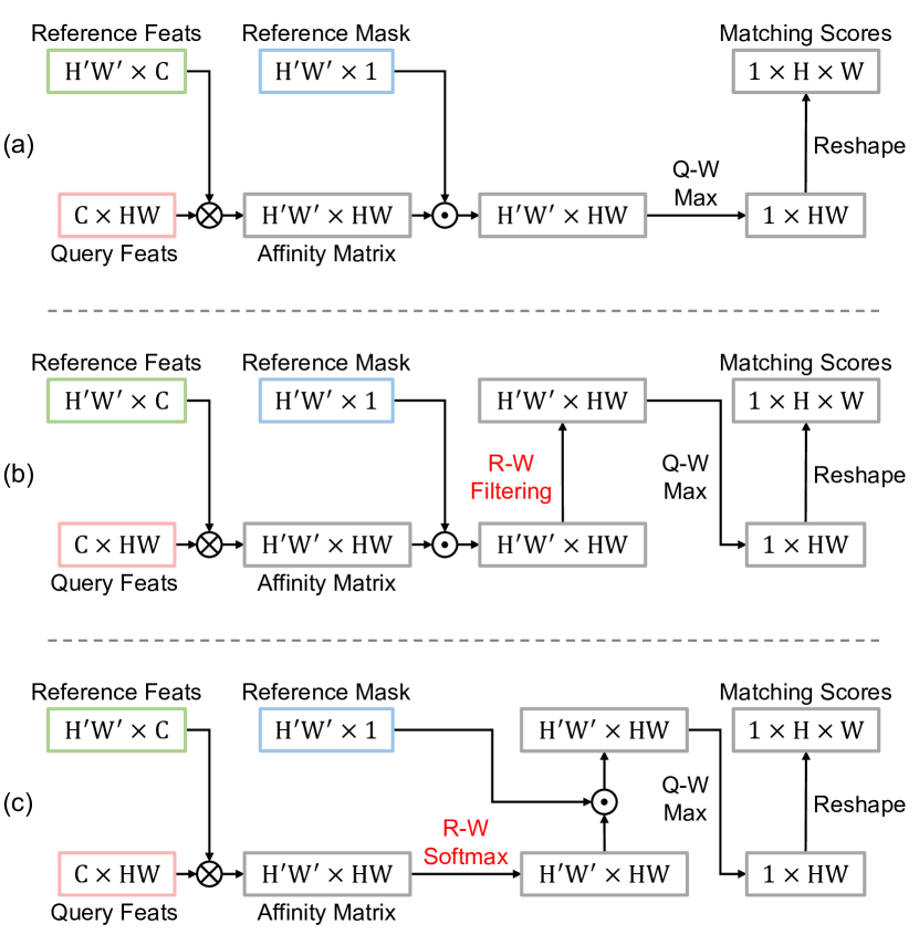
Figure 2: Comparison between (a) surjective matching, (b) bijective matching, and (c) equalized matching. Q-W and R-W indicate query-wise and reference-wise operations, respectively.

3.3 Bijective Matching

Instead of providing absolute options to the query frame, the options of both the reference frame and the query frame should be considered to better deal with the background distractions. To this end, KMN [35] and BMVOS [5] introduce bijective matching methods that dynamically restrict the query frame options for stricter and more reliable information transfer. Before the query-wise maximum operation, a pre-defined filtering map, such as a Gaussian kernel or a top K mask, is multiplied to the class-embodied affinity matrix $B$, i.e., $A_{BG}$ or $A_{FG}$, as

$$B_{p}\leftarrow f(p)\odot B_{p}~{},$$ (3)

where $f$ indicates the filter generation function that outputs the values from 0 to 1. As the query frame options are now partial rather than absolute, the matching scores can be implemented to follow the pre-defined design goals, e.g., excluding distant pixels from the best-matching pixel or discarding pixels except best-matching K pixels. The pipeline of bijective matching is also visualized in Figure 2 (b).

Although bijective matching methods can reflect reference frame options in the feature similarity scores, they can only be adopted at the testing stage replacing surjective matching, as they are based on discrete functions that restrain stable network training. Therefore, they cannot be used jointly with surjective matching that has different advantages to bijective matching. Furthermore, test-time manual tuning is required for searching the optimal hyper-parameter settings.

3.4 Equalized Matching

To overcome these limitations of the existing bijective matching methods while maintaining the same objective, we design a novel matching method that is totally independent to surjective matching and still can capture bijectiveness during feature matching. Here, we introduce an equalized matching mechanism that is fully differentiable, and therefore, can stand alone as a bold branch or be used with surjective matching simultaneously. As in surjective matching and bijective matching, feature similarity between $p$ and $q$ is first computed as

$$sim\left(p,q\right)=X^{k}_{p}\cdot X^{i}_{q}~{}.$$ (4)

Based on the feature similarity, the affinity matrix $A$ can be calculated as before. Then, to impress the bijectiveness in the affinity matrix itself, a softmax operation is performed along the query dimension as

$$A_{p}\leftarrow Softmax(A_{p})~{}.$$ (5)

Through this process, the sum of all query frame pixels’ scores becomes 1 for each reference frame pixel, i.e., all reference frame pixels have the same contribution to the query frame prediction. Therefore, if a reference frame pixel is referenced a lot, its scores will be lowered as they should divide up the same pie. Considering that such confusing reference frame pixels may cause critical errors, strictly suppressing their matching scores is an effective strategy for minimizing visual distractions. After modulating the affinity matrix $A$, the remaining process is implemented just as in surjective matching, as described in Figure 2 (c).

Unlike existing bijective matching methods, the proposed equalized matching mechanism does not contain discrete functions, so it can be stably learned during the network training stage as an independent branch. It can play the same role as bijective matching methods but does not suffer from the same problems as them. First, it can be flexibly plugged on top of surjective matching as well as used alone, enabling a full exploitation of surjective matching. Second, test-time manual tuning is not required as no hyper-parameters are needed.

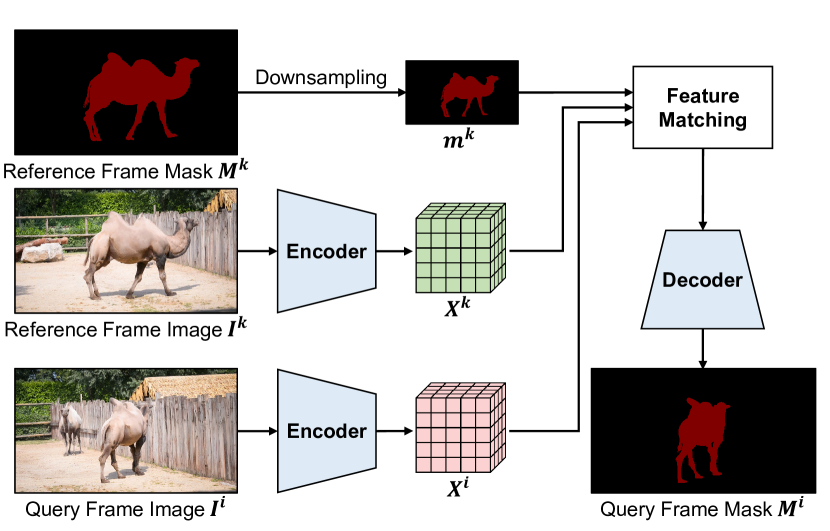
Figure 3: Architecture of our proposed method. The query frame is matched to the reference frame using the selected matching method. For simplicity and better understanding, mask propagation and skip connections are omitted in the illustration.

3.5 Network Architecture

Our network is based on a simple encoder–decoder architecture as illustrated in Figure 3. At the query frame, embedded features are first extracted from an image using an encoder. Then, those features are compared to the reference frame features via feature similarity matching. As reference frames, initial frame and previous adjacent frames are selected. For feature matching, we use surjective matching and equalized matching simultaneously, instead of transforming surjective matching to bijective matching at test time. This enables our network to capture flexibility as well as reliability through a visual matching process. Finally, by decoding the embedded features with the generated four score maps, query frame mask can be inferred.

3.6 Implementation Details

Encoder. We use DenseNet-121 [13], which is pre-trained on ImageNet [17], as our backbone network. It can be broadly divided into three blocks, which output 1/4-, 1/8-, and 1/16-scaled feature maps compared to the input image resolution. Only the 1/16-scaled feature maps are used for feature similarity matching.

Decoder. The decoder is designed identically to TBD [6]. It consists of convolutional layers that fuse and refine different features, and deconvolutional layers [49] that upscale the refined features. For fast decoding, every deconvolutional layer outputs only two channels to reduce the computational complexity. Before every deconvolutional layer, CBAM [41] is added to reinforce feature representations.

Table 1: Quantitative evaluation on the DAVIS 2016 validation set. OL denotes online learning. (+S) denotes the use of static image datasets during the network training.

Method	OL	fps	$\mathcal{G}_{\mathcal{M}}$	$\mathcal{J}_{\mathcal{M}}$	$\mathcal{F}_{\mathcal{M}}$
STCNN (+S) [43]		0.26	83.8	83.8	83.8
FEELVOS (+S) [38]		2.22	81.7	80.3	83.1
RANet (+S) [40]		30.3	85.5	85.5	85.4
DTN (+S) [51]		14.3	83.6	83.7	83.5
STM (+S) [31]		6.25	86.5	84.8	88.1
DIPNet (+S) [11]		0.92	86.1	85.8	86.4
CFBI (+S) [47]		5.56	86.1	85.3	86.9
GC (+S) [20]		25.0	86.6	87.6	85.7
KMN (+S) [35]		8.33	87.6	87.1	88.1
STG-Net (+S) [26]		-	85.7	85.4	86.0
RMNet (+S) [42]		11.9	81.5	80.6	82.3
HMMN (+S) [36]		10.0	89.4	88.2	90.6
EMVOS (+S)		49.8	88.4	87.9	88.9
RANet [40]		30.3	-	73.2	-
FRTM [34]	✓	21.9	81.7	-	-
BMVOS [5]		45.9	82.2	82.9	81.4
EMVOS		49.8	86.0	86.7	85.3

3.7 Network Training

Pre-training on static images. Following the existing VOS solutions [40, 31, 20, 22, 36], we simulate videos by augmenting static images to obtain diverse network training samples. To this end, an image segmentation dataset COCO [24] is used. For each image sample, simulated video sequence is generated by augmenting the source image. The simulated video sequence has 5 frames, i.e., a source image and 4 sequentially-augmented images.

Main training on videos. After pre-training the network on the simulated samples, the network is trained on either the DAVIS 2017 [33] training set or the YouTube-VOS 2018 [44] training set depending on the target testing dataset. During this main training stage, we randomly sample 10 consecutive frames.

Detailed settings. In all training stages, video frames are randomly cropped to have 384$\times$384 resolution. For stable network training, balanced random cropping is adopted as in CFBI [47] and TBD [6]. To provide challenging but natural training samples, the swap-and-attach augmentation is applied with a probability of 20%, as in TBD. The learning rate is set to 1e-4 without learning rate decay, and Adam optimizer [16] is used. Batch normalization layers [14] are also frozen following common protocol.

Table 2: Quantitative evaluation on the DAVIS 2017 validation set. OL denotes online learning. (+S) denotes the use of static image datasets during the network training.

Method	OL	fps	$\mathcal{G}_{\mathcal{M}}$	$\mathcal{J}_{\mathcal{M}}$	$\mathcal{F}_{\mathcal{M}}$
STCNN (+S) [43]		0.26	61.7	58.7	64.6
FEELVOS (+S) [38]		2.22	69.1	65.9	72.3
DMM-Net (+S) [50]		-	70.7	68.1	73.3
AGSS-VOS (+S) [23]		10.0	67.4	64.9	69.9
RANet (+S) [40]		30.3	65.7	63.2	68.2
DTN (+S) [51]		14.3	67.4	64.2	70.6
STM (+S) [31]		6.25	71.6	69.2	74.0
DIPNet (+S) [11]		0.92	68.5	65.3	71.6
LWL (+S) [2]	✓	14.0	74.3	72.2	76.3
CFBI (+S) [47]		5.56	74.9	72.1	77.7
GC (+S) [20]		25.0	71.4	69.3	73.5
KMN (+S) [35]		8.33	76.0	74.2	77.8
AFB-URR (+S) [22]		4.00	74.6	73.0	76.1
STG-Net (+S) [26]		-	74.7	71.5	77.9
RMNet (+S) [42]		11.9	75.0	72.8	77.2
LCM (+S) [10]		8.47	75.2	73.1	77.2
SSTVOS (+S) [8]		-	78.4	75.4	81.4
HMMN (+S) [36]		10.0	80.4	77.7	83.1
EMVOS (+S)		49.8	79.0	76.9	81.2
AGSS-VOS [23]		10.0	66.6	63.4	69.8
STM [31]		6.25	43.0	38.1	47.9
FRTM [34]	✓	21.9	68.8	66.4	71.2
TVOS [52]		37.0	72.3	69.9	74.7
JOINT [30]	✓	4.00	78.6	76.0	81.2
BMVOS [5]		45.9	72.7	70.7	74.7
EMVOS		49.8	75.6	73.8	77.5

4 Experiments

The datasets and evaluation metrics used in this study are described in Section 4.1. Quantitative comparison to the state-of-the-art VOS solutions can be found in Section 4.2. To validate our proposed approach, we analyze each proposed component thoroughly in Section 4.3. Note that our method is abbreviated as EMVOS and all our experiments are implemented on a single GeForce RTX 2080 Ti GPU.

4.1 Experimental Setup

Datasets. We use the DAVIS [32, 33] and YouTube-VOS [44] datasets to validate our proposed approach. DAVIS 2016 and DAVIS 2017 respectively contain 50 and 120 video sequences having 24 fps. YouTube-VOS 2018 is the largest dataset for VOS, comprising 3,945 video sequences having 30 fps. All frames are annotated in the DAVIS datasets, while every five frames are annotated in the YouTube-VOS dataset.

Evaluation metrics. We use intersection-over-union (IoU) to evaluate the segmentation performance. $\mathcal{J}$ measure denotes the IoU for the entire region of an object, while $\mathcal{F}$ measure denotes the IoU for only the boundaries of an object. $\mathcal{G}$ measure, which is the average of $\mathcal{J}$ and $\mathcal{F}$, is used as the primary measure for evaluating VOS performance.

Table 3: Quantitative evaluation on the DAVIS 2017 test-dev set. OL denotes online learning. (+S) denotes the use of static image datasets during the network training.

Method	OL	fps	$\mathcal{G}_{\mathcal{M}}$	$\mathcal{J}_{\mathcal{M}}$	$\mathcal{F}_{\mathcal{M}}$
OSVOS-S (+S) [29]	✓	0.22	57.5	52.9	62.1
CNN-MRF (+S) [1]	✓	0.03	67.5	64.5	70.5
DyeNet (+S) [19]	✓	0.43	68.2	65.8	70.5
PReMVOS (+S) [28]	✓	0.03	71.6	67.5	75.7
FEELVOS (+S) [38]		2.22	54.4	51.2	57.5
AGSS-VOS (+S) [23]		10.0	57.2	54.8	59.7
RANet (+S) [40]		30.3	55.3	53.4	57.2
STG-Net (+S) [26]		-	63.1	59.7	66.5
EMVOS (+S)		49.8	67.5	65.4	69.6
AGSS-VOS [23]		10.0	54.3	51.5	57.1
TVOS [52]		37.0	63.1	58.8	67.4
BMVOS [5]		45.9	62.7	60.7	64.7
EMVOS		49.8	64.0	61.9	66.1

4.2 Quantitative Results

DAVIS. We compare our method to other state-of-the-art methods on the DAVIS [32, 33] datasets in Table 1, Table 2, and Table 3. On all datasets, the inference speed is calculated on the DAVIS 2016 validation set, and 480p resolution is used. If static image datasets are used for network training, EMVOS achieves the second place on the DAVIS 2016 validation set and DAVIS 2017 validation set. On the DAVIS 2017 test-dev set, it is only outperformed by the online learning-based DyeNet [19] and PReMVOS [28], which are significantly slower than our method. If only the DAVIS training set is used for network training, EMVOS outperforms all other methods on the DAVIS 2016 validation set and DAVIS 2017 test-dev set. Considering its high inference speed of 49.8 fps, EMVOS shows the best speed–accuracy trade-off among all existing VOS methods on the DAVIS datasets.

Table 4: Quantitative evaluation on the YouTube-VOS 2018 validation set. (+S) denotes the use of static image datasets during the network training.

Method	fps	$\mathcal{G}_{\mathcal{M}}$	$\mathcal{J}_{\mathcal{S}}$	$\mathcal{J}_{\mathcal{U}}$	$\mathcal{F}_{\mathcal{S}}$	$\mathcal{F}_{\mathcal{U}}$
STM (+S) [31]	-	79.4	79.7	72.8	84.2	80.9
SAT (+S) [3]	39.0	63.6	67.1	55.3	70.2	61.7
LWL (+S) [2]	-	81.5	80.4	76.4	84.9	84.4
EGMN (+S) [27]	-	80.2	80.7	74.0	85.1	80.9
CFBI (+S) [47]	-	81.4	81.1	75.3	85.8	83.4
GC (+S) [20]	-	73.2	72.6	68.9	75.6	75.7
KMN (+S) [35]	-	81.4	81.4	75.3	85.6	83.3
RMNet (+S) [42]	-	81.5	82.1	75.7	85.7	82.4
LCM (+S) [10]	-	82.0	82.2	75.7	86.7	83.4
GIEL (+S) [9]	-	80.6	80.7	75.0	85.0	81.9
SwiftNet (+S) [39]	-	77.8	77.8	72.3	81.8	79.5
SSTVOS (+S) [8]	-	81.7	81.2	76.0	-	-
JOINT (+S) [30]	-	83.1	81.5	78.7	85.9	86.5
HMMN (+S) [36]	-	82.6	82.1	76.8	87.0	84.6
AOT-T (+S) [48]	41.0	80.2	80.1	74.0	84.5	82.2
AOT-L (+S) [48]	16.0	83.8	82.9	77.7	87.9	86.5
STCN (+S) [4]	-	83.0	81.9	77.9	86.5	85.7
RPCMVOS (+S) [45]	-	84.0	83.1	78.5	87.7	86.7
EMVOS (+S)	28.6	79.7	79.3	74.3	83.4	81.7
RVOS [37]	22.7	56.8	63.6	45.5	67.2	51.0
A-GAME [15]	-	66.1	67.8	60.8	-	-
AGSS-VOS [23]	12.5	71.3	71.3	65.5	76.2	73.1
CapsuleVOS [7]	13.5	62.3	67.3	53.7	68.1	59.9
STM [31]	-	68.2	-	-	-	-
FRTM [34]	-	72.1	72.3	65.9	76.2	74.1
TVOS [52]	37.0	67.8	67.1	63.0	69.4	71.6
STM-cycle [21]	43.0	69.9	71.7	61.4	75.8	70.4
BMVOS [5]	28.0	73.9	73.5	68.5	77.4	76.0
EMVOS	28.6	78.6	78.5	73.1	82.5	80.3

YouTube-VOS. The comparison of our method and other state-of-the-art methods on YouTube-VOS 2018 [44] validation set is presented in Table 4. If external training data is adopted, heavy networks with a growing memory pool, such as RPCMVOS [45], AOT [48], JOINT [30], and STCN [4], show notable performance. EMVOS achieves a comparable inference speed and segmentation accuracy to a lite version of AOT, with 28.6 fps and a $\mathcal{G}$ score of 79.7%. Under the constraint of not using the external datasets, EMVOS outperforms all previous methods by a large margin, with a $\mathcal{G}$ score of 78.6%. This supports the exceptional generalization ability of EMVOS; performance degradation is only 1.1% while that of STM [31] is 11.2%.

Table 5: Comparison of various model versions with various feature matching methods. SM, BM, and EM indicate surjective matching, bijective matching, and equalized matching, respectively. K1 and K2 indicate the hyper-parameters (kernel standard deviation or number of pixels to be filtered) for bijective matching with the initial and previous adjacent frames. The models are tested on the DAVIS 2017 validation set.

Version	Matching	K1	K2	$\mathcal{G}_{\mathcal{M}}$
Baseline	SM	-	-	75.7
1	SM $\rightarrow$ BM (Kernel)	16	32	76.5
1	SM $\rightarrow$ BM (Kernel)	32	32	77.5
1	SM $\rightarrow$ BM (Kernel)	64	32	76.5
1	SM $\rightarrow$ BM (Kernel)	32	16	77.3
1	SM $\rightarrow$ BM (Kernel)	32	64	77.3
6	SM $\rightarrow$ BM (Top K)	64	16	74.4
6	SM $\rightarrow$ BM (Top K)	128	16	76.2
6	SM $\rightarrow$ BM (Top K)	256	16	75.9
6	SM $\rightarrow$ BM (Top K)	128	8	74.5
6	SM $\rightarrow$ BM (Top K)	128	32	75.9
11	EM	-	-	77.9
12	SM + EM	-	-	79.0

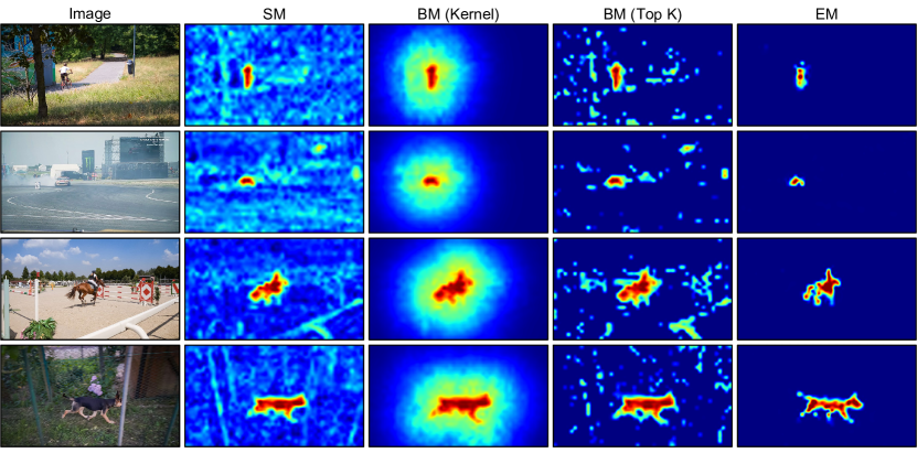
Figure 4: Comparison of the feature matching results obtained by various matching methods. SM, BM, and EM indicate surjective matching, bijective matching, and equalized matching, respectively. For a clear visualization, the values in each score map are linearly normalized to be in the same range.

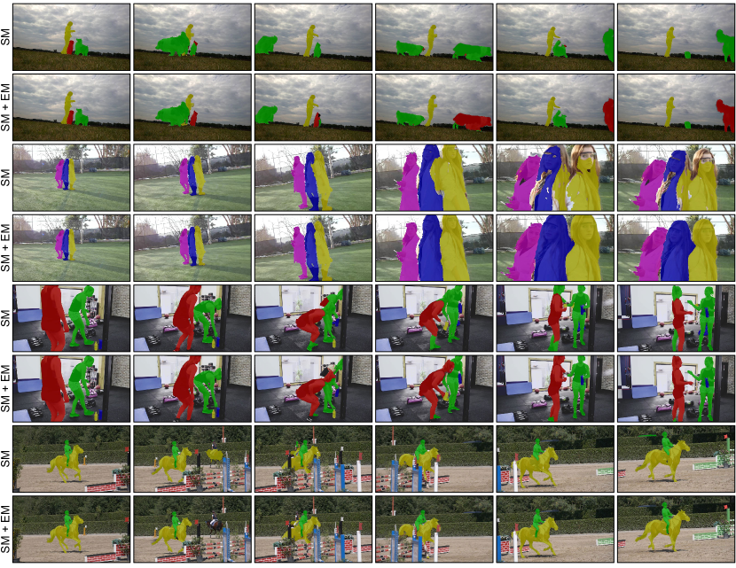
Figure 5: Qualitative segmentation mask comparison of the models using various matching methods. SM and EM indicate surjective matching and equalized matching, respectively.

4.3 Analysis

Qualitative matching comparison. To validate the effectiveness of our proposed equalized matching mechanism, we qualitatively compare the matching score maps of various matching methods in Figure 4. As a naive surjective matching only considers the query frame options, all query frame pixels can make their best choices. Therefore, background distractions as well as the foreground object have high matching scores, which prevents a clear distinction between foreground and background. For a better separation of foreground and background, bijective matching methods apply some filtering strategies to surjective matching at test time. The kernel-based bijective matching method [35] can restrict the search area by applying a Gaussian kernel, but the score maps are quite coarse and blurred because of the nature of the kernelling. The top K-based bijective matching method [5] can suppress the background scores to some extent, but still suffers from noisy background distractors. By contrast, our proposed equalized matching method can clearly distinguish foreground objects from the background while maintaining fine details. Specifically, in the third and the fourth sequences, the thin parts of the horse and dog (tails and legs) are not well captured in surjective matching, kernel-based bijective matching, and top K-based bijective matching. However, in equalized matching, they can be well captured as information transfer is performed in a more strict and reliable manner.

Quantitative mask comparison. We also compare various matching methods with respect to their final segmentation performance. In Table 5, various model versions with various matching methods are quantitatively compared. The baseline model is a model employing naive surjective matching. It achieves a $\mathcal{G}$ score of 75.7%. By adopting Gaussian kernelling or a top K selection to the baseline model at test time, further improvements can be achieved. The kernel-based bijective matching can bring up to 1.8% performance improvement, and the top K-based bijective matching can boost up to 0.5% on $\mathcal{G}$ metric. However, as can be seen from the table, bijective matching methods are quite sensitive to the hyper-parameter values. Consequently, they require an extra process for searching optimal hyper-parameters via test-time manual tuning, but this makes the solution less elegant and efficient. The proposed equalized matching method achieves a $\mathcal{G}$ score of 77.9%, which surpasses the optimal performance of the bijective matching methods without the need for manual tuning. As well as being able to stand alone, it can also be used on top of surjective matching. If surjective matching and equalized matching are used together, the performance exceeds all other matching methods by a large margin, demonstrating the effectiveness of their joint use.

Qualitative mask comparison. In Figure 5, output segmentation masks of model versions with various matching methods are qualitatively compared. The baseline model only uses surjective matching, while our final model leverages both surjective matching and equalized matching. In the first and the third sequences, the baseline model misses the red object because red and green objects look similar. As there is no limitation to the information-referencing process in surjective matching, the red object can get a high ”green object score”, which leads to the red object getting missed. In the second sequence, where the three target objects are visually similar, the baseline model fails to accurately segment the objects, especially for boundaries of the objects. This is because surjective matching is susceptible to confusing information, so the boundary regions that have relatively unclear features are not handled well. In the fourth sequence, wrong detection of the background distractors is also observed, as they have similar appearance to the target objects. Only employing surjective matching is proven to make the network vulnerable to the visual distractions. By contrast, our final model can effectively deal with all these sequences, thanks to its strong ability to distinguish foreground objects from the background via reliable and stable information propagation.

5 Conclusion

To improve the conventional surjective matching mechanism for VOS, bijective matching methods have been proposed, but these have certain limitations as well. To overcome them while maintaining the same objective, we introduce an equalized matching mechanism. The effectiveness of the proposed equalized matching mechanism is thoroughly validated via extensive experiments. By simply adopting surjective matching and equalized matching with a naive encoder–decoder architecture, we achieve the best speed–accuracy trade-off on public benchmark datasets. We believe our approach will be widely used in future research.

References

- [1] Linchao Bao, Baoyuan Wu, and Wei Liu. Cnn in mrf: Video object segmentation via inference in a cnn-based higher-order spatio-temporal mrf. In Proceedings of the IEEE conference on computer vision and pattern recognition, pages 5977–5986, 2018.
- [2] Goutam Bhat, Felix Järemo Lawin, Martin Danelljan, Andreas Robinson, Michael Felsberg, Luc Van Gool, and Radu Timofte. Learning what to learn for video object segmentation. In European Conference on Computer Vision, pages 777–794. Springer, 2020.
- [3] Xi Chen, Zuoxin Li, Ye Yuan, Gang Yu, Jianxin Shen, and Donglian Qi. State-aware tracker for real-time video object segmentation. In Proceedings of the IEEE/CVF Conference on Computer Vision and Pattern Recognition, pages 9384–9393, 2020.
- [4] Ho Kei Cheng, Yu-Wing Tai, and Chi-Keung Tang. Rethinking space-time networks with improved memory coverage for efficient video object segmentation. Advances in Neural Information Processing Systems, 34, 2021.
- [5] Suhwan Cho, Heansung Lee, Minjung Kim, Sungjun Jang, and Sangyoun Lee. Pixel-level bijective matching for video object segmentation. In Proceedings of the IEEE/CVF Winter Conference on Applications of Computer Vision, pages 129–138, 2022.
- [6] Suhwan Cho, Heansung Lee, Minhyeok Lee, Chaewon Park, Sungjun Jang, Minjung Kim, and Sangyoun Lee. Tackling background distraction in video object segmentation. arXiv preprint arXiv:2207.06953, 2022.
- [7] Kevin Duarte, Yogesh S Rawat, and Mubarak Shah. Capsulevos: Semi-supervised video object segmentation using capsule routing. In Proceedings of the IEEE/CVF International Conference on Computer Vision, pages 8480–8489, 2019.
- [8] Brendan Duke, Abdalla Ahmed, Christian Wolf, Parham Aarabi, and Graham W Taylor. Sstvos: Sparse spatiotemporal transformers for video object segmentation. In Proceedings of the IEEE/CVF Conference on Computer Vision and Pattern Recognition, pages 5912–5921, 2021.
- [9] Wenbin Ge, Xiankai Lu, and Jianbing Shen. Video object segmentation using global and instance embedding learning. In Proceedings of the IEEE/CVF Conference on Computer Vision and Pattern Recognition, pages 16836–16845, 2021.
- [10] Li Hu, Peng Zhang, Bang Zhang, Pan Pan, Yinghui Xu, and Rong Jin. Learning position and target consistency for memory-based video object segmentation. In Proceedings of the IEEE/CVF Conference on Computer Vision and Pattern Recognition, pages 4144–4154, 2021.
- [11] Ping Hu, Jun Liu, Gang Wang, Vitaly Ablavsky, Kate Saenko, and Stan Sclaroff. Dipnet: Dynamic identity propagation network for video object segmentation. In Proceedings of the IEEE/CVF Winter Conference on Applications of Computer Vision, pages 1904–1913, 2020.
- [12] Yuan-Ting Hu, Jia-Bin Huang, and Alexander G Schwing. Videomatch: Matching based video object segmentation. In Proceedings of the European conference on computer vision (ECCV), pages 54–70, 2018.
- [13] Gao Huang, Zhuang Liu, Laurens Van Der Maaten, and Kilian Q Weinberger. Densely connected convolutional networks. In Proceedings of the IEEE conference on computer vision and pattern recognition, pages 4700–4708, 2017.
- [14] Sergey Ioffe and Christian Szegedy. Batch normalization: Accelerating deep network training by reducing internal covariate shift. arXiv preprint arXiv:1502.03167, 2015.
- [15] Joakim Johnander, Martin Danelljan, Emil Brissman, Fahad Shahbaz Khan, and Michael Felsberg. A generative appearance model for end-to-end video object segmentation. In Proceedings of the IEEE Conference on Computer Vision and Pattern Recognition, pages 8953–8962, 2019.
- [16] Diederik P Kingma and Jimmy Ba. Adam: A method for stochastic optimization. arXiv preprint arXiv:1412.6980, 2014.
- [17] Alex Krizhevsky, Ilya Sutskever, and Geoffrey E Hinton. Imagenet classification with deep convolutional neural networks. Communications of the ACM, 60(6):84–90, 2017.
- [18] Mingxing Li, Li Hu, Zhiwei Xiong, Bang Zhang, Pan Pan, and Dong Liu. Recurrent dynamic embedding for video object segmentation. In Proceedings of the IEEE/CVF Conference on Computer Vision and Pattern Recognition, pages 1332–1341, 2022.
- [19] Xiaoxiao Li and Chen Change Loy. Video object segmentation with joint re-identification and attention-aware mask propagation. In Proceedings of the European Conference on Computer Vision (ECCV), pages 90–105, 2018.
- [20] Yu Li, Zhuoran Shen, and Ying Shan. Fast video object segmentation using the global context module. In European Conference on Computer Vision, pages 735–750. Springer, 2020.
- [21] Yuxi Li, Ning Xu, Jinlong Peng, John See, and Weiyao Lin. Delving into the cyclic mechanism in semi-supervised video object segmentation. Advances in Neural Information Processing Systems, 33:1218–1228, 2020.
- [22] Yongqing Liang, Xin Li, Navid Jafari, and Jim Chen. Video object segmentation with adaptive feature bank and uncertain-region refinement. Advances in Neural Information Processing Systems, 33:3430–3441, 2020.
- [23] Huaijia Lin, Xiaojuan Qi, and Jiaya Jia. Agss-vos: Attention guided single-shot video object segmentation. In Proceedings of the IEEE International Conference on Computer Vision, pages 3949–3957, 2019.
- [24] Tsung-Yi Lin, Michael Maire, Serge Belongie, James Hays, Pietro Perona, Deva Ramanan, Piotr Dollár, and C Lawrence Zitnick. Microsoft coco: Common objects in context. In European conference on computer vision, pages 740–755. Springer, 2014.
- [25] Zhihui Lin, Tianyu Yang, Maomao Li, Ziyu Wang, Chun Yuan, Wenhao Jiang, and Wei Liu. Swem: Towards real-time video object segmentation with sequential weighted expectation-maximization. In Proceedings of the IEEE/CVF Conference on Computer Vision and Pattern Recognition, pages 1362–1372, 2022.
- [26] Daizong Liu, Shuangjie Xu, Xiao-Yang Liu, Zichuan Xu, Wei Wei, and Pan Zhou. Spatiotemporal graph neural network based mask reconstruction for video object segmentation. In Proceedings of the AAAI Conference on Artificial Intelligence, volume 35, pages 2100–2108, 2021.
- [27] Xiankai Lu, Wenguan Wang, Martin Danelljan, Tianfei Zhou, Jianbing Shen, and Luc Van Gool. Video object segmentation with episodic graph memory networks. In Computer Vision–ECCV 2020: 16th European Conference, Glasgow, UK, August 23–28, 2020, Proceedings, Part III 16, pages 661–679. Springer, 2020.
- [28] Jonathon Luiten, Paul Voigtlaender, and Bastian Leibe. Premvos: Proposal-generation, refinement and merging for video object segmentation. In Asian Conference on Computer Vision, pages 565–580. Springer, 2018.
- [29] K-K Maninis, Sergi Caelles, Yuhua Chen, Jordi Pont-Tuset, Laura Leal-Taixé, Daniel Cremers, and Luc Van Gool. Video object segmentation without temporal information. IEEE transactions on pattern analysis and machine intelligence, 41(6):1515–1530, 2018.
- [30] Yunyao Mao, Ning Wang, Wengang Zhou, and Houqiang Li. Joint inductive and transductive learning for video object segmentation. In Proceedings of the IEEE/CVF International Conference on Computer Vision, pages 9670–9679, 2021.
- [31] Seoung Wug Oh, Joon-Young Lee, Ning Xu, and Seon Joo Kim. Video object segmentation using space-time memory networks. In Proceedings of the IEEE/CVF International Conference on Computer Vision, pages 9226–9235, 2019.
- [32] Federico Perazzi, Jordi Pont-Tuset, Brian McWilliams, Luc Van Gool, Markus Gross, and Alexander Sorkine-Hornung. A benchmark dataset and evaluation methodology for video object segmentation. In Proceedings of the IEEE Conference on Computer Vision and Pattern Recognition, pages 724–732, 2016.
- [33] Jordi Pont-Tuset, Federico Perazzi, Sergi Caelles, Pablo Arbeláez, Alexander Sorkine-Hornung, and Luc Van Gool. The 2017 davis challenge on video object segmentation. arXiv:1704.00675, 2017.
- [34] Andreas Robinson, Felix Jaremo Lawin, Martin Danelljan, Fahad Shahbaz Khan, and Michael Felsberg. Learning fast and robust target models for video object segmentation. In Proceedings of the IEEE/CVF Conference on Computer Vision and Pattern Recognition, pages 7406–7415, 2020.
- [35] Hongje Seong, Junhyuk Hyun, and Euntai Kim. Kernelized memory network for video object segmentation. In European Conference on Computer Vision, pages 629–645. Springer, 2020.
- [36] Hongje Seong, Seoung Wug Oh, Joon-Young Lee, Seongwon Lee, Suhyeon Lee, and Euntai Kim. Hierarchical memory matching network for video object segmentation. In Proceedings of the IEEE/CVF International Conference on Computer Vision, pages 12889–12898, 2021.
- [37] Carles Ventura, Miriam Bellver, Andreu Girbau, Amaia Salvador, Ferran Marques, and Xavier Giro-i Nieto. Rvos: End-to-end recurrent network for video object segmentation. In Proceedings of the IEEE/CVF Conference on Computer Vision and Pattern Recognition, pages 5277–5286, 2019.
- [38] Paul Voigtlaender, Yuning Chai, Florian Schroff, Hartwig Adam, Bastian Leibe, and Liang-Chieh Chen. Feelvos: Fast end-to-end embedding learning for video object segmentation. In Proceedings of the IEEE/CVF Conference on Computer Vision and Pattern Recognition, pages 9481–9490, 2019.
- [39] Haochen Wang, Xiaolong Jiang, Haibing Ren, Yao Hu, and Song Bai. Swiftnet: Real-time video object segmentation. In Proceedings of the IEEE/CVF Conference on Computer Vision and Pattern Recognition, pages 1296–1305, 2021.
- [40] Ziqin Wang, Jun Xu, Li Liu, Fan Zhu, and Ling Shao. Ranet: Ranking attention network for fast video object segmentation. In Proceedings of the IEEE international conference on computer vision, pages 3978–3987, 2019.
- [41] Sanghyun Woo, Jongchan Park, Joon-Young Lee, and In So Kweon. Cbam: Convolutional block attention module. In Proceedings of the European conference on computer vision (ECCV), pages 3–19, 2018.
- [42] Haozhe Xie, Hongxun Yao, Shangchen Zhou, Shengping Zhang, and Wenxiu Sun. Efficient regional memory network for video object segmentation. In Proceedings of the IEEE/CVF Conference on Computer Vision and Pattern Recognition, pages 1286–1295, 2021.
- [43] Kai Xu, Longyin Wen, Guorong Li, Liefeng Bo, and Qingming Huang. Spatiotemporal cnn for video object segmentation. In Proceedings of the IEEE/CVF Conference on Computer Vision and Pattern Recognition, pages 1379–1388, 2019.
- [44] Ning Xu, Linjie Yang, Yuchen Fan, Dingcheng Yue, Yuchen Liang, Jianchao Yang, and Thomas Huang. Youtube-vos: A large-scale video object segmentation benchmark. arXiv preprint arXiv:1809.03327, 2018.
- [45] Xiaohao Xu, Jinglu Wang, Xiao Li, and Yan Lu. Reliable propagation-correction modulation for video object segmentation. In Proceedings of the AAAI Conference on Artificial Intelligence, volume 36, pages 2946–2954, 2022.
- [46] Xiaohao Xu, Jinglu Wang, Xiang Ming, and Yan Lu. Towards robust video object segmentation with adaptive object calibration. arXiv preprint arXiv:2207.00887, 2022.
- [47] Zongxin Yang, Yunchao Wei, and Yi Yang. Collaborative video object segmentation by foreground-background integration. In European Conference on Computer Vision, pages 332–348. Springer, 2020.
- [48] Zongxin Yang, Yunchao Wei, and Yi Yang. Associating objects with transformers for video object segmentation. Advances in Neural Information Processing Systems, 34, 2021.
- [49] Matthew D Zeiler, Graham W Taylor, and Rob Fergus. Adaptive deconvolutional networks for mid and high level feature learning. In 2011 International Conference on Computer Vision, pages 2018–2025. IEEE, 2011.
- [50] Xiaohui Zeng, Renjie Liao, Li Gu, Yuwen Xiong, Sanja Fidler, and Raquel Urtasun. Dmm-net: Differentiable mask-matching network for video object segmentation. In Proceedings of the IEEE/CVF International Conference on Computer Vision, pages 3929–3938, 2019.
- [51] Lu Zhang, Zhe Lin, Jianming Zhang, Huchuan Lu, and You He. Fast video object segmentation via dynamic targeting network. In Proceedings of the IEEE/CVF International Conference on Computer Vision, pages 5582–5591, 2019.
- [52] Yizhuo Zhang, Zhirong Wu, Houwen Peng, and Stephen Lin. A transductive approach for video object segmentation. In Proceedings of the IEEE/CVF Conference on Computer Vision and Pattern Recognition, pages 6949–6958, 2020.