Physical configurations of a cell doublet with line tension, a theoretical study.
Fabrice Delbary
Collège de France, 11 Place Marcelin-Berthelot, 75231 Paris Cedex 05, France
1 Introduction
Although being a very simple configuration, a cell doublet can appear to be very useful in force inference. First when studying microcsopy images of cell doublets. After segmentation, measurements of the angles at the cells junction allow to have estimates of the cell surface tensions (up to a common scaling factor). Second, instead of measuring the different quantities after segmentation, one can use an adjoint method where using an iterative scheme, the cell doublet is segmented while imposing the physical equation verified by the cells, this method allows to get more precise estimates of the tensions. For these practical applications, exact formulae or at least as precise as possible are needed. Finally, the cell doublet can also be used as a toy model to test more general force inference algorithms by using quasi exact data coming from the cell doublet. In this framework, it is important to be able to compute the solution(s) to the cell doublet very precisely, these data can then be pertubated with artificial noise in order to estimate which level of error makes the general force inference algorithms fail. Changing the parameters of the toy model can also allow to exhibit problematic configurations for the force inference algorithm. For a cell doublet with surface tensions only, it is well-known that simple considerations of geometry give the angles between forces [2, 4, 7, 10, 14]. Thus, no hard work is required to test some force inference algorithms on exact data. Things are diferent if one is now also interested in the height of the cells junction for instance, since it depends on the tensions and the model constraints (e.g. volume contraints); the same holds for the cell centre positions. Hence, it is quite interesting to get an anlytical formula for these other configuration parameters. The first part of this work is dedicated to this problem. Although almost the different results for a cell doublet with surface tensions are known, we choose to present them in this document. It allows us to introduce the polynomial way to formulate the problem, which appears particularly useful in the third part of this work when a line tension is introduced. Thus, for a better understanding, we prove the different results by starting from scratch. More precisely, considering a cell doublet defined by its geometrical parameters, we derive the Young-Laplace and Young-Dupré laws by minimizing its surface energy under volume constraints, the angles between forces are then uniquely defined. The other geometrical parameters of the configuration (height of the cell junction and position of the centres) can then be found using the volume equations. Finally, obtaining precisely the parameters of the cell doublet configuration is not such a hard task since it only sums up to solve a small optimization problems with four parameters and two volume constraints which can be done very efficently and very precisely in a numerical way. Moreover, since the energy of the constrained system has a unique minimum, optimization algorithms converge to it even the initial guess is slightly changed. As previously mentioned though, anaytical formulae can be convenient to get extremely precise data, specially close the limit cases where optimization algorithms may be slow to converge.
In a second part, we show how to compute the geometrical parameters of a cell doublet with surface tensions when the pressures instead of the volumes are known. This case does not present any difficulty since the Young-Laplace and Young-Dupré laws immmediately give simple relations between the geometrical parameters and the tensions and pressures.
In the third part of this document, we consider a cell doublet with surface tensions and a line tension. At first sight, it is not obvious if the system has only one or several energy minima. Hence, if there are several, an optimization algorithm would end at only one of them and the computed minimum would highly depends on the initial guess. Moreover, if no information on the number of local minima is known, it makes difficult the task to find the global minimum. Somewhat in between the case of a unique minimum and the case of several minima, we study in a quantitative way, a cell doublet with line tension and volume constraints, which has the property to have three obvious local minima (when the cell junction disappears) and apparently a unique other local minimum (if the tensions allow it) which is a critical point of the energy.
2 Description
We consider two cells and joined by an interface and want to study the configuration of the system at minimum energy. The cell surfaces are modelized as three spherical caps , , with respective centers , , , where defines the interface and where the surface of cell is given by . We consider the oriented axis whose origin is the center of the base circle of and whose direction is given by the vector . We denote by (respectively ), the unit circle (respectively unit disk) of center orthogonal to .
For and , we denote by the spherical cap with base circle and apex . is defined as the disk . The surfaces are then given by , , for with .
Remark 2.1.
For , define the same spherical caps, hence the same configuration of the cell doublet, but it is more convenient to keep it this way than restraining .
One might want to introduce the radii of the spherical caps as well as their aperture in order to express in a more common way the force balance. Hence, we define for
| (1) |
For sake of simplicity, the cosines and sines are abbreviated for as
| (2) |
We then have for
| (3) |
The tension of each surface is respectively denoted by . Note that the angles of tension forces with respect to the axis are respectively biven by , . The volumes of cells and are respectively given by
| (4) | ||||
| (5) |
Which can also be written with the vaiables as
| (6) | ||||
| (7) |
Or with the vaiables as
| (8) | ||||
| (9) |
We define the difference of angles by
| (10) |
Where indices are considered modulo (in ), that is , etc.. These angles satisfy
| (11) |

3 Configuration at minimum energy under volume constraints
For constrained volumes, the pressure forces exert no work under a change of configuration and the energy of the system is simply given by the sum of surface tensions times the spherical caps areas, that is
| (12) |
That is
| (13) |
Where
| (14) |
Note that the energy can also be written using the or variables and we have
| (15) |
| (16) |
3.1 Equations for the critical points of the constrained energy
Since the problem of finding the critical points of the energy is purely algebraic (all the equations are given by polynomials), although not mandatory, it is interesting to describe it in an algebraic way. You can refer to [5, 12, 15, 16], but as a quick reminder, and rougly speaking, an affine variety is an implicit manifold whose defining equations are polynomials. It can happen that the affine variety has singularities (it is not a manifold at these points), the dimension of an affine variety is however defined as its maximal dimension at regular points when viewed as a manifold. To end this very short, incomplete and non exhaustive presentation, an ideal is a set of polynomials which is a group for the sum and such that the multiplication of a polynomial in the ideal by any other polynomial (not necessary in the ideal) is sill in the ideal. Hence, zeros of a polynomial system can also be characterized as the zeros of the ideal generated by the polynomials of the system (smallest ideal containing the polynomials).
We consider the problem of finding the minimizer of the energy (or equivalently ) under volume constraints and , where , that is, we want to find the minimizer of the polynomial on the affine variety of dimension of defined by the ideal where are given by
| (17) | ||||
| (18) |
Where for , . We also denote and . Note that is implicitely imposed by the volume constraints.
Remark 3.1.
An homothety of the surface tensions does not change the configuration of the system at minimum energy. Similarly, an homothety of factor of the volumes simply scales the spatial coordinates of the system at minimum energy by a factor , thus, the angles remain unchanged.
Remark 3.2.
It is an easy task to solve numerically the problem and find the configuration of the double cell. However, we would like to have explicit formulae that could be used directly. Since the problem has been written in terms of a minimization of a polynomial on an affine variety, the solution will hence be given as the solution to polynomial system. Using a Gröbner basis [15] (computed for instance with a Computer Algebra System like Singular [8]), the solution is then simply given by taking the successive roots of polynomials whose coefficients depend on the previous parameters given by the previous polynomials. However, note that although semi-explicit, this way of solving the system is not the most appropriate for numerical applications since Gröbner basis often give large polynomial coefficients which can dramatically destroy the precision. Nonetheless, in our simple case of a double cell, we can easily find an univariate polynomial whose only real root is one of the parameter . The other parameters are then given by Möbius transformations depending on the surface tensions and can be computed using the volumes and the parameters.
Remark 3.3.
For , the polynomial has a unique real root given by
| (19) |
Which can also be written
| (20) |
Where
| (21) |
Hence, can be easily paramaterized using and one of the other three variabes , indeed, is any of the set of points respectively defined by
| (22a) | |||
| (22b) | |||
| (22c) | |||
The limit is well-defined as , giving in fact parameterizations of the closed subvariety of of points with (algebraic curve of the hyperplane ), that is, the points such that
The respective parameterizations are given by
| (23) | ||||
| (24) | ||||
| (25) |
Remark that is a positive definite quadratic form of and is closed, hence the minimum on is reached at some point. Moreover, it can be easily checked that the singular locus of is empty, thus the minimum of on is a critical point. The singular locus of is the set points of which are singular, that is points such that is not a differentiable manifold at these locations, the tangent plane has not dimension anymore, that is, if we denote by and by the Jacobian of (basis of the orthogonal to the tangent plane), these points vanish the minors of and of course the polymomials of since the points have to be on the variety. The ideal generated by these polynomials can then be written
| (26) |
That is
| (27) | ||||
We can see that the zeros of are quadruples such that for a couple , hence .
We now want to find the critical points of the constrained energy. These points are characterized as those such that the gradient of the energy is orthogonal to tangent plane to , that is, the gradient of the energy lies in the space generated by . This is exactly what is done when working with the Lagrangian . Deriving it, we search for the points and the coefficients (pressures) such that can be written as a combination of the vectors in the orthogonal of the tangent place, that is .
We can also proceed by searching for the points of vanishing the minors of the gradient of , the critical ideal of the volume constrained energy (polynomials whose zeros are the critical points of the constrained energy) is then given by
| (28) |
That is
| (29) | ||||
Hence, the algebraic degree of the problem is (number of zeros of the critical ideal in ), however, most of critical points are without interest for our considerations since they are either complex or do not correspond to a minimum of the constrained energy but to a maximum or a saddle point. But we can already see that for , any critical point of the constrained energy has to verify the volume constraints and
| (30) | ||||
| (31) |
That is
| (32) | ||||
| (33) |
Which is the force balance on the junction circle (Young-Dupré law) [2, 4, 7, 10, 14]. It shows in particular that , , can not have the same sign (no non-physical moon-shape configuration for the system). Geometrically speaking, since the sum of tension forces is , they form a triangle whose lengths are . This implies that is uniquely determined up to a minus sign. In addition, since we have because of volume constraints (cell on the left and cell on the right), we then have and which determines the sign of . Moreover, as we will detail later, the tensions have to fulfill the triangle inequalities.


Still considering a possible critical point with , the triangle formed by the tension forces has angles , and the law of cosines (dot product of each couple of forces) gives for
| (34) | ||||
| (35) |
The law of sines gives for
| (36) | ||||
| (37) |
For , denoting , we thus get the law of cotangents
| (38) |
Remark 3.4.
For , we have , so that we recover the well-known property asserting that the tension forces at the junction circle form angles.
Remark 3.5.
For , the condition of criticality is given by
That is
As intuitively expected, we will see that only one of the first three conditions correspond to a configuration of minimum energy, namely exclusion or inclusion which happens when one of the surface tension is greater than the sum of the two others.
3.2 A more physical but equivalent way to proceed: the Lagrangian
In fact, physics laws may appear more clearly when working (equivalently) with Lagrange multipliers as mentioned earlier, indeed, reaches its minimum in at a point vanishing the gradient of the Lagrangian where are Lagrange multipliers (relative pressures inside each cell). Assuming and deriving with respect to and , we easily get the pressures.
| (39) | ||||
| (40) |
Giving respectively the Young-Laplace law for the spherical caps and [2, 4, 7, 10, 14]. Deriving with respect to and and replacing by the values of and , we get as previously the force balance on the junction circle (30) giving (32) when expressed in terms of angles. Note that the sine relation of (32) also gives the Young-Laplace law for the spherical cap and the property . Finally, finding the minimum of the energy under volume constraints amounts to seek for the solutions of the following system with unknown
| (41a) | ||||
| (41b) | ||||
| (41c) | ||||
| (41d) | ||||
And to seek for the minimum of the constrained energy for . One of the points is then the global minimizer.
3.3 Externalization and internalization
Consider a critical point of the constrained energy and assume that . Then the force balance at the cells junction (41a,41b) implies that the three tension forces form a triangle whose lengths are , which can only occur if these lengths fulfill the triangle inequalities for all . In fact, the inequalities are strict, indeed, if for a , then the force balance implies which is forbidden by the volume constraints.
Hence, if for a given , the tension satisfies , then the constrained energy has no critical point in and the global minimum, as well as any local minimum, is reached on . In fact, we can intuitively guess that the tension pulls until surface completely disappears, which leads to internalization of cell in cell if , to internalization of cell in cell if and to externalization if . Mathematically speaking, we will prove that the constrained energy has no other minimizer than the externalized/internalized configuration corresponding to the triangle inequality which is violated (mutually exclusive cases). We will also prove that these configurations are not local minimizers of the constrained energy on when the triangle inequalities are fulfilled.
Remark 3.6.
The three triangle inequalities for all can be written more concisely as
Where we recall that . It can also be written in the following way, for a chosen
In this case, the similar inequalities fulfilled by the other are a consequence of the previous one.
Keep on considering general . First, on , the only minimizers of the energy are the points given by or or , that is, the points defined by
| (42a) | ||||
| (42b) | ||||
| (42c) | ||||
Indeed, on , considering for instance the parameterization in given in (23), we have with defined for by
| (43) |
For , we have ( is concave on each interval) and for , . Hence, on , the energy has local minima only at the points . Since , at least one of these points is a global minimizer of the energy on , hence also on if .
Second, using the Hessian of the constrained energy, one can see which points are possible minimizers. Using the parameterizations of given in (22a), we have
Hence, for , can be a local minimizer on only if and is for sure one if inequality is strict. Thus, if , none of the points can be a local minimizer of the energy on , hence neither a global one. Moreover, for , since the energy has its global minimizer among and since the conditions on the tensions are mutually exclusive, it has only one local minimizer on which is also the global one.
Remark 3.7.
The latter holds if for , . In this case, the Hessian matrix at is positive but not definite, however, since the Hessian matrices at and are not positive and since the global minimizer of the energy is among , it is necessarily .
To summarize, we have
-
•
If , the energy on has no local minimizer located on .
- •
If , then reaches its global minimum at (which is also the unique minimizer), corresponding to the configuration of cell internalized in cell . We then have , , .

Figure 3: Cell internalized in cell . - •
If , then reaches its global minimum at (which is also the unique minimizer), corresponding to the configuration of cell internalized in cell . We then have , , .

Figure 4: Cell internalized in cell . - •
If , then reaches its global minimum at (which is also the unique minimizer), corresponding to the configuration of separated cells and . We then have , , .

Figure 5: Separated cells and . - •
Remark 3.8.
For all , if the point is not the global minimizer of the constrained energy, then it is a saddle point. The energy has two other critical points for that we did not take into account since they are not minimizers. As it can be seen with the function defined in (43), one of these critical point is such that and the other one is such that . In can be easily checked that these points are local maxima of the energy.
3.4 Non-degenerate case
As previously mentioned, for , any local minimizer of the constrained energy is a critical point in . Hence, consider a critical point of the energy in and . We will prove that can be uniquely written in terms of , that can be uniquely written in terms of , and that is the root of a degree polynomial. We will then prove that the polynomial has a unique real root which shows that the constrained energy has a unique critical point (up to the sign of which does not change the doublet configuration) which is also the unique local and global minimizer.
For convenience, we define a notation of the volumes, similar to the difference of angles.
First, from the volume constraints, we have
| (44) |
Second, since , are obtained by Möbius transformations of
Moreover, from volume constraints, we have
Hence, replacing by their expression in terms of we get where the polynomial is defined by
| (45) |
Where and are defined by
| (46) | ||||
| (47) |
In the following, for sake of simplicity in the notations, for a chosen , we simply denote . The variables with subscript are denoted with a subscript, that is .
3.4.1 Uniqueness of the local/global minimum
Since the polynomial defined in (45) has roots in , there are a priori five critical points of the energy under volume constraints, one of them being the global minimum. However, as we are going to prove, the polynomial has a unique real root so that the energy has a unique critical point which is also its global minimizer. The other parameters of the configuration at minimum energy are then given by
Theorem 3.9.
The polynomial defined in (45) has a unique real root.
Proof.
, hence for , if and only if
That is, if and only if
| (48) |
Where and the rational fraction is defined by
| (49) |
Where the polynomials (with no root in ) are defined by
The derivative of is given by
Where the polynomial is defined by
Where
Since , we have , thus for all , we have so that is a strictly increasing function. Moreover . Thus, is a bijection from to , that is, for all , there exists a unique such that . In particular, taking proves the theorem. ∎
Remark 3.10.
Theorem 3.9 also proves that for strictly positive volumes (what we assume), the unique real root of has multiplicity . Indeed, the only possible roots having multiplicity larger than are . Since , is a proper Möbius transform (not constant) and the unique respective preimages of and are and which are not roots of .
We can summarize the different cases which can appear in a double cell with constrained volumes by the fact that there always exists a unique local minimum of the energy, which is then the global minimum of the system. When the tensions fulfill the triangle inequality, the configuration of the system can be found by solving a degree equation which has a unique real root. For the cases where the tensions do not fulfill the triange inequality, one of the surfaces disappear depending on which tension is larger than the sum of the two others. These results can be visualized on the following graph.

Remark 3.11.
We cannot expect a closed fomula in terms of radicals giving the roots of defined in (45) (in particular the real one). Indeed, it is well-known that there is no solution in radicals to general polynomial equations of degree [6]. To check that is not a special polynomial which can be solved by radicals, consider as indeterminates and as an element of . and are coprime in , hence also and are. Moreover, hence is irreducible in . Since is monic in , from Gauss lemma, is irreducible in , hence in . Thus the Galois group of is a transitive subgroup of . can be computed with a computer algebra system and we have exactly so that is not solvable by radicals. Hence, from Hilbert irreducibility theorem, polynomials obtained by specializing in for are “almost always” irreducible. In fact, a consequence of this theorem is that the Galois group of the specialized polynomial is “almost always” isomorphic to the Galois group of over which is so that the specialization is not solvable by radicals.
Consider the simple case where , in this case we specialize the polynomial in . Then denote , that is
Reasoning as previously shows that is irreducible in and that its Galois group is as well, so that the polynomials obtained by specializing in for are “almost always” irreducible and that the Galois group of the specialized polynomial is “almost always” isomorphic to the Galois group of over which is , so that the specialization is not solvable by radicals. In fact, in this particular case, all specializations such that is irreducible in produce as Galois group. Moreover, the values of for which is reducible can be explicitely determined, they are the values of for which has a rational root. Indeed, if for , factorizes as polynomials of respective degree and , has obviously a rational root. Now , if for , factorizes as polynomials of respective degree and in , one can check that we have necessarily (it corresponds to or ) and
In particular, has a rational root.
The values of such that has a root in can be easily expressed since is linear in , they are
And in this case
It is in fact possible to get closed formulae for the roots of a general polynomial of degree , one has however to use a Tschirnhaus transformation [17] to write the quintic in its principal form or in its Bring-Jerrard form [3, 9]. In the first case, one has to solve the associated icosahedral equation [11, 13] whose roots can be expressed in terms of hypergeometric functions [1]. In the second case, the roots can be written in terms of Jacobi theta functions or hypergeometric functions [1]. However, although theoretically interesting, these formulae are quite cumbersome and are often not the most appropriate way to solve the problem for numerical applications.
3.4.2 A few words about infering the tensions
Consider the problem of expressing (up to a common scaling factor) in terms of the angles . We present here some laws which can be useful for force inference. Generally well-known, some of them are quite obvious, some others a bit more complicated. If we consider the law of sines (36), then defining by the circumradius of the triangle defined by the tension forces, we have
So that for
Which is in fact Lamé law when expressed without the factor
| (50) |
We immediately get a similar relations for the cosines simply by writing for , . We can also write the tensions using the three angles and the perimeter by using the following expression linking the circumradius, the perimeter and the three angles
We then get for
Where
Lamé law again follows by dividing each by for . A similar expression for the cosines immediately follows, but we can also get it from the law of cosines (34) and we have for
This gives in terms of sines of the half angles, for
The relation for the cosines of the half angles immediately follows. We can also write the tensions in terms of the perimeter using the law of cotangents (38) and we have all .
3.4.3 Configuration of the cell doublet for given pressures
We propose now to express the parameters of a cell doublet when the surface tensions veryfing the triangle equation and when the pressures are known. Then from the Young-Laplace law and the sine relation of the Young-Dupré law
| (51) | |||
| (52) | |||
| (53) |
Where . Hence, the cosine relation of the Young-Dupré law implies that
| (55) |
Hence
| (56) |
Since fulfill the triangle inequality, the right hand side is always positive. Choosing , we then have
| (57) |
The parameters can then be otained by solving the sine relations (51), giving
| (58) | ||||
| (59) | ||||
| (60) |
Note that we do not have continuity to when in the coordinate if the minus sign is chosen, we have instead . Remark also that the signs can not be chosen independently since have to fulfill the cosine relation
| (61) |
More precisely, denoting by
| (62) |
We have two possible triples of solutions for , denoted by and . They are given by
| (63) | ||||
| (64) | ||||
| (65) |
Where the posible solution is the one such that the third coordinate lacks continuity to as . We will see that the triple does not solve the problem anyway. To solve it, the first coordinate of the triple should be negative, the second one should be positive and the third one between both. We already know that and since they respectively have the sign of and . Now, we have
| (66) | ||||
| (67) | ||||
| (68) | ||||
| (69) |
Moreover
| (70) | |||
| (71) |
Hence, we always have whereas when , we have and when , we have . Thus, for all positive surface tensions fulfilling the triangle inequality and for all positive pressures , there exists a configration of the cell doublet, this configuration is unique and given by the parameters previously computed.
4 Cell doublet with line tension
We consider the same problem as in section 3 except that we now assume that the system has a line tension along the junction circle. Then, the energy is now defined as
Where is the line tension and we recall, . We now restrict the problem to (otherwise we can put an absolute value in the energy). is positive and , moreover, the semialgebraic set is closed, hence reaches its minimum on , either at a critical point on or on .
4.1 Equations for the critical points of the constrained energy
With the same notations as in section 3.1, the critical ideal of the energy on the affine variety is given by
| (73) | ||||
The algebraic degree of the problem is . We can see that the energy has no critical point such that . However, since is now the boundary of the domain of the constrained energy, points such that do not need to be critical points to be local extrema. The zeros of the critical ideal fufill the modified Young-Dupré law
| (74) | ||||
| (75) |
And the volumes contraints. One can again work the Lagrangian of the energy to recover this results. Making the derivatives of with respect to vanish, we get the Laplace law on the surfaces
| (76) | ||||
| (77) | ||||
| (78) |
And the modified Young-Dupré law previously mentioned. Before tackling the local extrema of the energy such that , consider first the case of points such that (points in ). Points which are local minima of the energy on are of course the same as in the problem 3.3 without line tension and they are those corresponding to internalization or externalization. In the presence of line tension, the three points are local minima of the energy, indeed, using the parameterizations of given in (22a), we have
| (79) | ||||
| (80) | ||||
| (81) |
We now want to find the local extrema of the energy of for . We need to solve the following system with known to find the critical points of the constrained energy
| (82) | ||||
| (83) | ||||
| (84) | ||||
| (85) |
In the case without line tension, the system is easier to solve because the three forces form a triangle whose angles are uniquely defined by its sides (surface tensions). However, we now have four forces forming a quadrilateral whose angles are not uniquely defined by its sides so that the two constraints equations play a role in the angles. As previously explained, we want to be sure to find the global minimum of the energy and the local minima as well, so the system can not be solved with Newton method. Computer Algebra Systems show some difficulties in finding a Gröbner basis for this system but as previously mentioned, they are often not the best solution. Hence, instead, we propose to solve the system using Polynomial Homotopy Continuation and to this end we use PHCpack [18]. We give the following polynomial system to the software
| (86a) | ||||
| (86b) | ||||
| (86c) | ||||
| (86d) | ||||
With unknowns , and where
| (87) |
One can also define
| (88) |
And solve the following system of unknowns instead
| (89) | ||||
Remark 4.1.
can be easily removed from the unknowns by using the value given by the first equation and replace in the two last equations. One then works with the three last equations and the unknowns . Note also that the two last equations can also be written as
Once the critical points are known, we need to determine if they are local minima, saddle points or local maxima. To this end, we use the Hessian of the Lagrangian with respect to . Indeed, consider a critical point , its associated Lagrange multipliers and the Hessian of with respect to the geometry taken at . Denote the tangent space to at , that is , where denotes the orthogonal.
-
•
If is a local maximum of the constrained energy, then for all .
If for all , then is a local maximum of the constrained energy. -
•
If changes sign for , then is a saddle point of the constrained energy.
-
•
If is a local minimum of the constrained energy, then for all
If for all , then is a local minimum of the constrained energy. -
•
If the Hessian is negative but not definite on the tangent space , more analysis is required to know if is a local maximum or a saddle point. Similarly, if the Hessian is positive but not definite on the tangent space , more analysis is required to know if is a local minimum or a saddle point.
Comparing the energy at the local minima and at the points , , one can find the global minimum of the constrained energy. To test the extremality of the critical points, we need the tangent space and the Hessian matrix . We recall that
| (90) |
Hence the following vectors form a basis of .
| (91) |
The Hessian matrix is simply given by
| (92) |
Hence, the Hessian matrix in the basis writes
| (93) |
Where
| (94) |
Thus, the matrix is positive if and only if its trace and its determinant are positive. The trace of is given by
| (95) |
And its determinant by
| (96) |
Where the determinant of is given by
| (97) |
We recall that the three local minima of for are given by (42a), (42b), (42c)
| (98) | ||||
| (99) | ||||
| (100) |
The energy at these points is
| (101) | ||||
| (102) | ||||
| (103) |
4.2 Theoretical and numerical results, observations
Remark first that like in the case of surface tensions only, different relations can be obtained from the balances of forces. More precisely, we have the following lemma
Lemma 4.2.
Assume that a volume constrained cell doublet with tensions and geometric parameters is at a local minimum of energy, then we recall that equations (86a) and (86b) are fulfilled (balances of forces).
We recall that for , we denote . Then for all
| (104a) | ||||
| (104b) | ||||
In particular, from (104a), we get
| (105) |
And for
| (106) |
That is
| (107) |
Proof.
4.2.1 Inequalities for tensions and volumes
We first propose to show an obvious inequality between the tensions and the inverse of the junction height .
Lemma 4.3.
If a cell doublet with tensions and geometric parameters is at a local minimum of energy, then, the balance of forces (equations (86a), (86b)) implies that three of the triangle inequalites the triangle inequality of the doublet without line tension is replaced by the quadrilateral inequality.
| (108) |
Proof.
We now propose to show a necessary condition on the tensions and volumes in order to have solutions to the system (86).
Lemma 4.4.
Proof.
Assume that the system (86) has a real solution . For , denote , then where for all
is symmetric, increasing on and decreasing on . Moreover, for all , , hence
Where we recall that . Hence
is positive on so that necessarily fulfills (110). Denote by and by the function . Since , then where
Hence . Moreover, reaches its maximum at where
Thus , with , that is
With
That is . Finally
Prove now the second inequality on the tensions. Consider and assume that . Then, using (104a), we have
The function is decreasing on , in addition, we have , hence
So that the second inequality is proved. ∎
4.2.2 Uniqueness of the interior minimum
After computing the critical points for a grid of parameters , there seems to be at most six critical points in the considered domain, more precisely, there are , , or . However, is seems that there is no local minimum when there are less than six critical points, whereas there is exactly one minimum when there are six critical points. Consequently, since when exists, the interior minimum is unique, a minimization algorithm could fit to search for the latter. However, there could be some difficulties to avoid the algorithm to converge to one of the three minima on the boundary of the domain (). This could probably be avoided by an appropriate choice of the initial guess. One can also remark that even when the energy has an interior minimum, this one is not mandatorily the global minimum of the system. In these cases, the global minimum is reached when , that is when for one of .
4.2.3 Energy and singularities
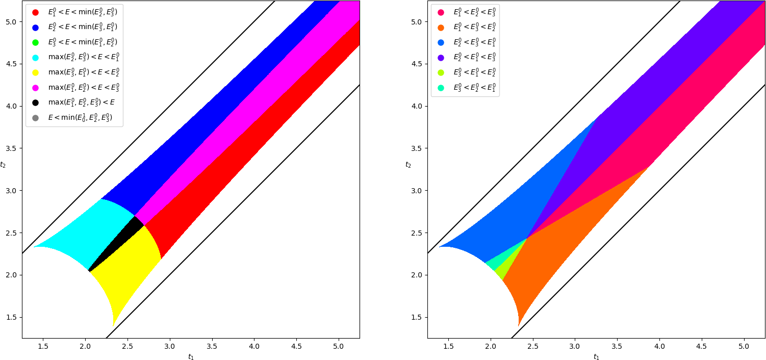
The singularities of the system are the critical points such that the determinant of the matrix (93) is , that is, the solutions to the system (86) such that Jacobian has determinant . For sake of simplicity, considering the reduced system (89), one can choose one of the parameters as being a new unknown (for instance ) and add the equation of vanishing Jacobian determinant to the system. Solving this new system for chosen tensions gives the singular points for these parameters as well as the corresponding volumes . However, not all singularities are of interest in our problem since they might occur for parameters which are not located at the boundary of the region where local minima are possible. Moreover, once computed, it is not convenient to check if a singularity is of interest or not.
Hence, for our numerical study, we proceed differently. Consider some parameters as fixed, for instance, like in the following, . Then, each couple of angles (that is ) uniquely determines such that the system (86) is fulfilled and the computation of these parameters is straightforward, indeed
| (112) | ||||
| (113) | ||||
| (114) | ||||
| (115) |
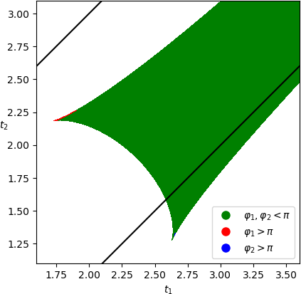
We have of course and . Then, if and and if the configuration is a local minimum, the couple can be recorded as being in the domain of existence of local minima for the energy. Processing a lot of couples of angles allow to have a fairly precise knowledge of the set of couples such that the energy has a local minimum.
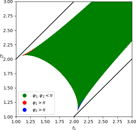
As a first example, we consider a surface tension and for different line tensions , we observe which surface tensions give rise to an interior minimum.
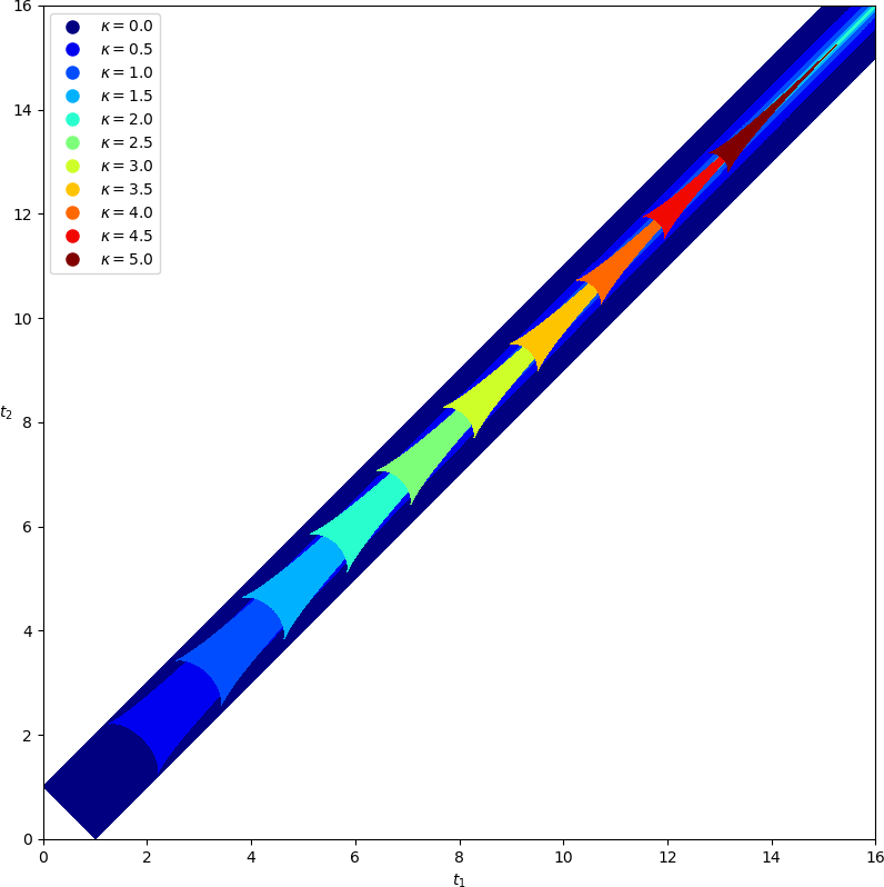
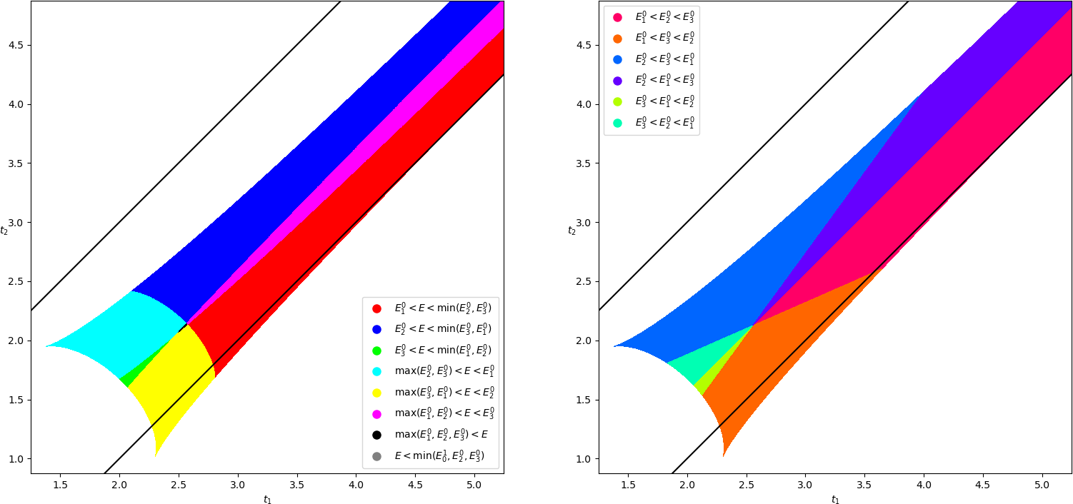
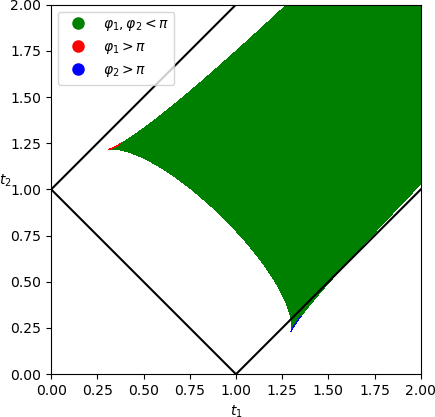
Fron sections 3.4 and 3.4.1, we already knew that for a doublet with only surface tensions, the domain of existence of a configuration does not depend on the volumes but only on the tensions (they have to fulfill the triangle inequalities). As expected, we can see that this is not true anymore for a doublet with line tension. Increasing the line tension also shrinks this domain. First unbounded, the domain becomes bounded when the line tension increases too much and then disappears when it is too high. When the cell volumes are not equal, we can also see that increasing the line tension slightly rotates the domain of existence of a configuration. We can observe these behaviours more into details and look at the value of the energy at the local minima. We still consider and we first consider equal volumes. For different values of the line tension , we again observe which surface tensions give rise to an interior minimum. For these local minima, we compare their energy to those of the three minima on the boundary. We denote by , the energy at .
Both on the domain of existence of a local minimum, the figure on the right shows the order of and the figure on the left compares the energy at the local minima to . For comparison with a doublet without line tension, the black solid line represents the location of tensions where the triangle inequalities are violated. As a reminder, this is the same plot as in figure 6. Inside the domain , a cell doublet without line tension has a unique configuration of minimum energy with junction height different than . Otherwise we either have internalization or externalization.
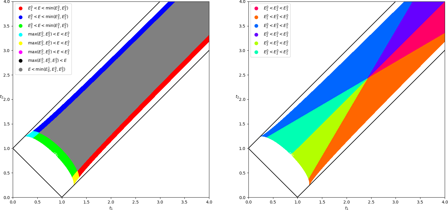
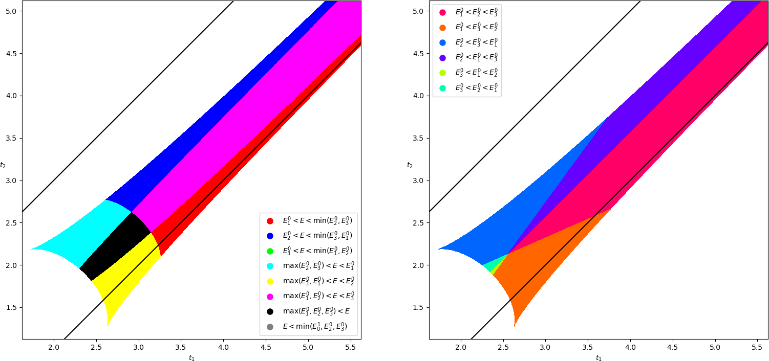
Hence, in this case, we can see that most of local minima are also global ones. However, things might be different, increasing the line tension makes the grey area become bounded and then decrease its size.
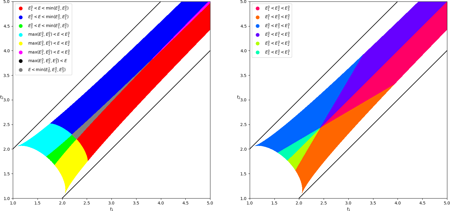
It finally disappears so that in these cases, despite the existence of a local minimum such that , the global minimum of the energy is always one of .
On the previous figures, the domain of tensions where a local minimum exists is in fact unbounded so that can be chosen arbitrarily large if they do not differ too much. The same holds true for a cell doublet without line tension. However, in the presence of line tension, the domain becomes bounded if increases too much. Precisely, in the case we are considering now (), it happens when
| (116) |
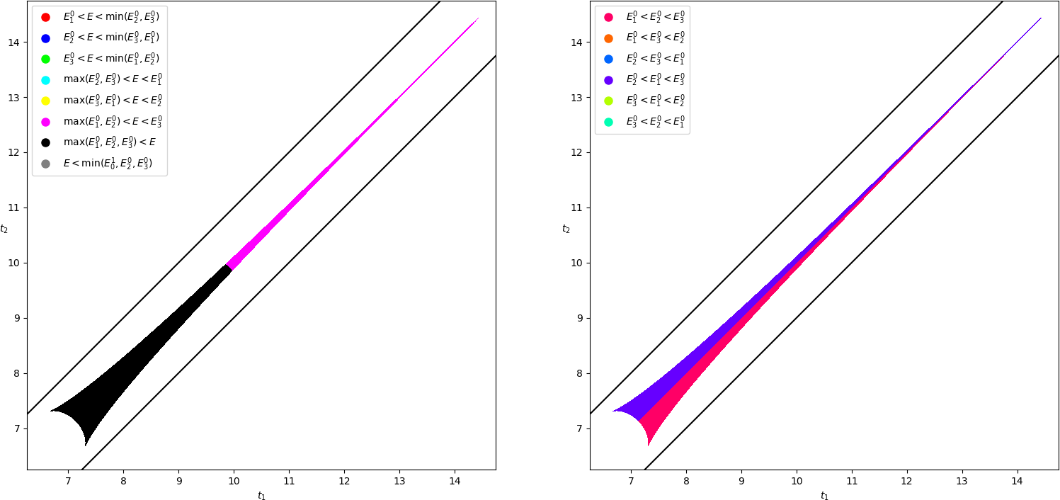
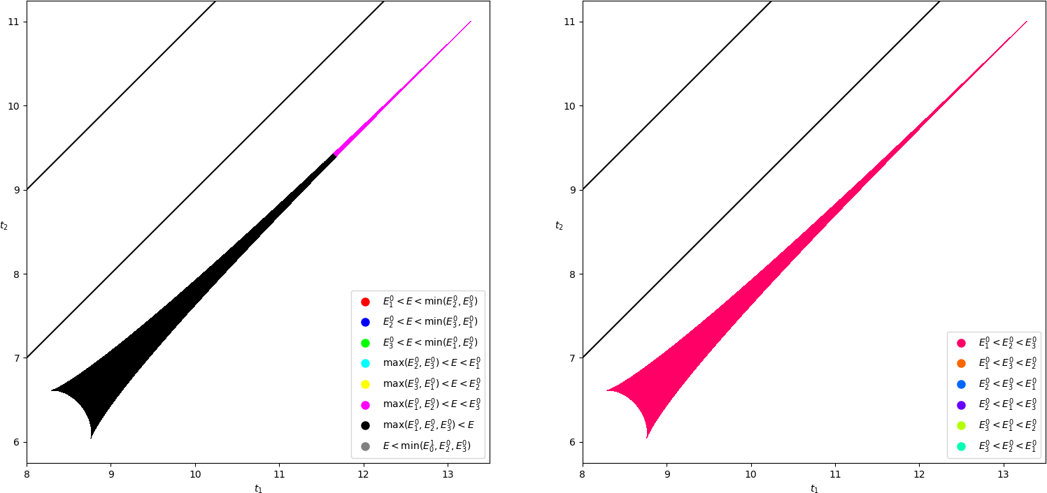
If increases more, then the energy of any local minimum is higher than the three energies for .
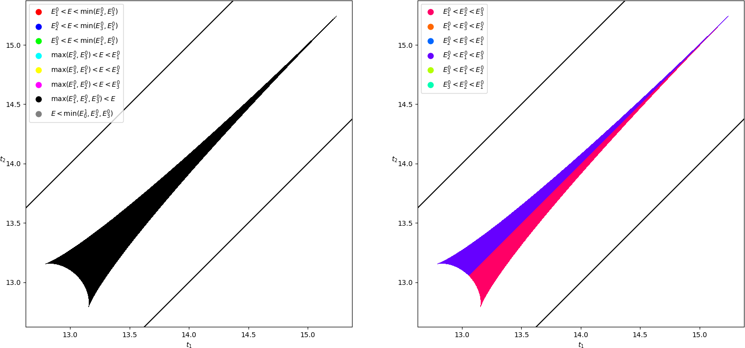
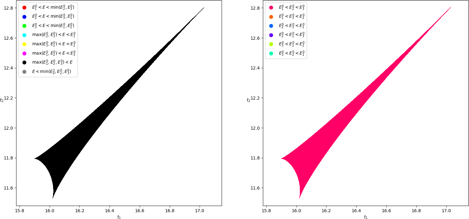
As increases, the set of couples such that the energy of a cell doublet has a local minimum is getting smaller and there is no more local minimum when is too large, more precisely when
| (117) |
Where we still consider the case . The common value of at the singularity (when equality holds in (117)) is given by
| (118) |
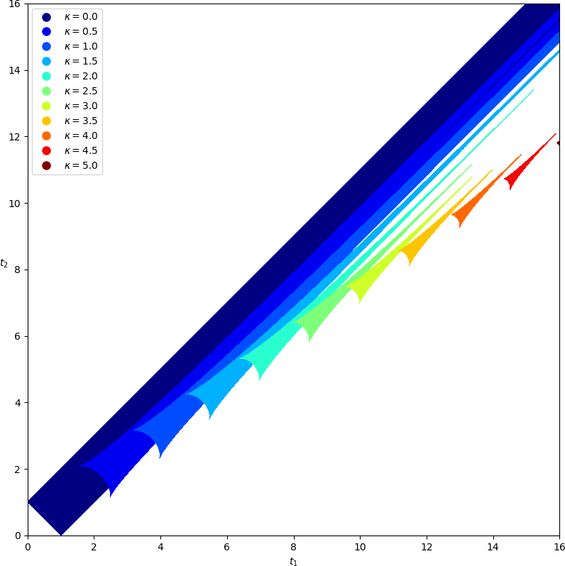
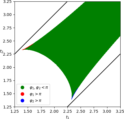
In all previous cases, the existence of a local minimum is implying that the surface tensions fulfill the triangle inequalities. However, there is a priori no reason for this fact to be true in general since we now have four forces (). Precisely, as already mentioned and seen on figure 7, contrary to the case of a doublet without line tension where singularities are independent of the volumes, they play a role if a line tension exists. Hence, to illustrate what happens in this case, consider for instance and, as previously, a constant surface tension and the same values of the line tension . We then get the following plots (the scales are different and have been chosen to fit the region of local minima in the best way).
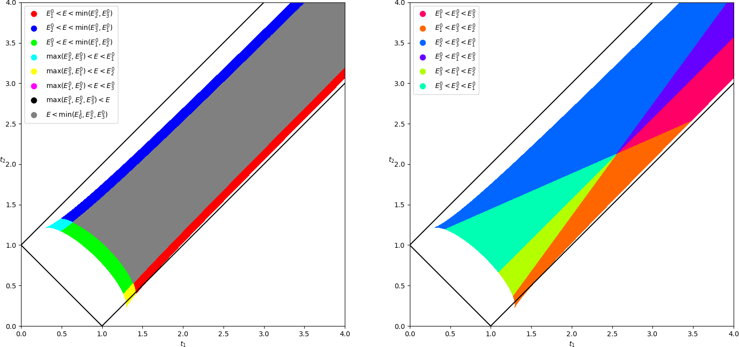
We can already remark that for some local minima, the surface tensions do not fulfill the triangle inequalities (the region of local minima is slightly “rotated”). This fact is even more obvious as the line tension increases.
For the two previous figures (“low” line tension ), besides the “rotation”, we can also remark that the region of local minima is slightly narrower compared to the previous case of equal volumes. This fact becomes more visible when increases. For , we get
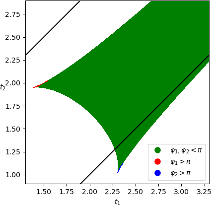
Now the surface tensions in the region of local minima never fulfill the triangle inequalities. Moreoever, the line tension for which the region becomes bounded has decreased compared to the equal volumes case. This value of can be expressed as the root of a polynomial but it is probably not possible to express it in terms of radicals though. Now, considering , we can again remark that the region of local minima is much smaller.
As in the equal volumes case, when increases enough, there is no more region of local minima. However, it happens for a lower line tension than in the equal volumes case. As previously mentionned, it may not be possible to express the location of this singularity in terms of radicals but it can be written as a root of a polynomial.
4.2.4 Bulging
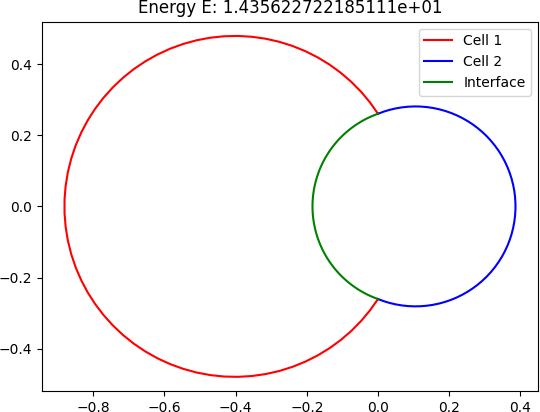
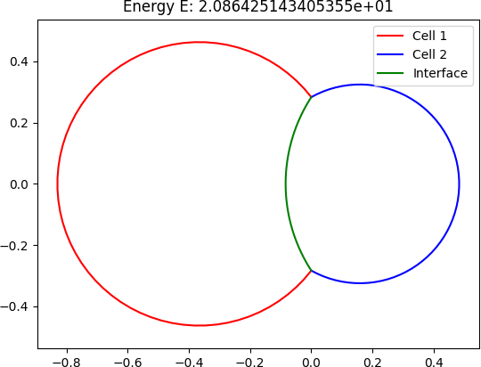
For a cell doublet without line tension, we necessarily have for all . It is possible to have (but with ) for a if the surface tension is small compared to the others. For instance, with equal volumes, we get the following configurations when two of the tensions are twenty times larger than the last one.
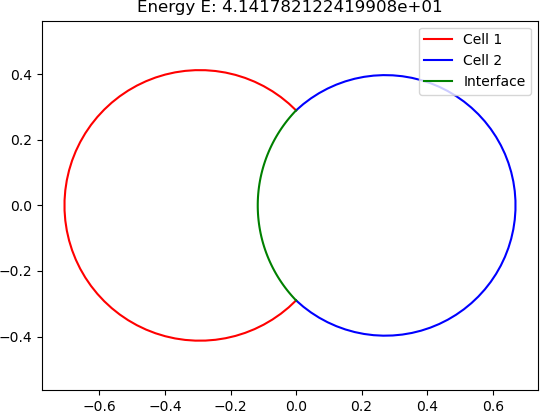
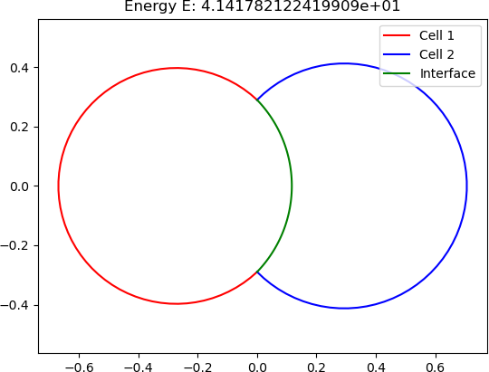
Now, this does not hold true anymore in the presence of line tension. Whereas we still have , one of the other angles may be slightly larger then . The cell doublet then looks like “bulged”. On the following figures, we can see for which tensions bulging happens. Consider the same examples as previously, first with equal volumes.
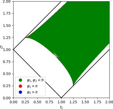
The area of bulging is rather small and located close to the boundary of the domain. For larger there is no more possible bulging. Since the region of bulging is very small and located close to the singularities, one can wonder if the previous results are not due to numerical errors. In order to be sure that this is not the case, one can check that the region of local minima can contain solutions such that or so that a slight modification of the tensions can lead to or . To do so, the system (86) can easily be solved exactly when assuming for instance . Indeed, we then have and the system writes
| (119) | ||||
| (120) | ||||
| (121) | ||||
| (122) |
Hence we immediately get
| (123) |
Replacing in the other equations, the first two can be used to find and the last one gives a condition on . We have
| (124) |
With
| (125) |
And
| (126) |
For equal volumes, , and (where bulging seems to happen), is then the largest real positive root of where
| (127) | ||||
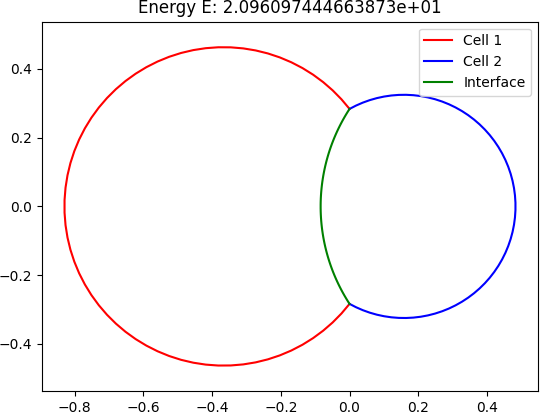
Using a Computer Algebra System, the different quantities can then be evaluated with arbitrary high precision. We get , , , , . The trace of the Hessian matrix is given by
and it determinant by . The configuration is then a local minimizer. By slightly decreasing ( maximum) or slightly increasing ( maximum), one then obtains a configuration such that which is a local minimizer. If we now look at what happens for different volumes (, ), we have similar results.
For larger , the area disappears first (it has almost disappeared for ), then the area disappears as well.
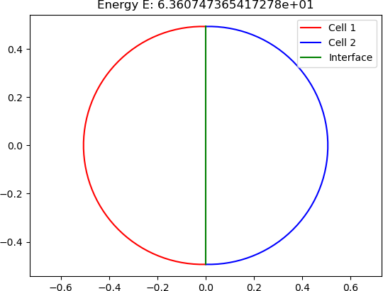
Running several computations with a large number of parameters, it seems that bulging is limited to about above flat angle. More important bulging which can be observed during some experiments may fit with the model though. Indeed, the case studied here is only a double cell and some things way differ when observing an early embryo for instance. We can also remark that the constaints (volume constraints here) play an important role in the configurations which can be observed. Different constraints may possibly lead to more important bulging. To end up with these remarks, bulging remarked in experiments can be due to other physical phenomenoms and/or combined effects of line tension studied here with something else. On the next figure, we can see how a double cell with maximum bulging appears. Precisely, we have .
4.2.5 Tension inference
As we have seen in section 3.4.2, for a doublet with only surface tensions, it is possible to infer the tensions (up to a common scaling factor). Moreover, from the previous section 4.2.4, line tensions have effects which make a configuration possibly differ from one without line tension. Thus, one can wonder if infering the tensions is possible in this more general case. In fact it seems to be an impossible task in general. Indeed, consider a doublet with parameters at local minimum. Of course, as in the case of double cells with only surface tensions, common scaling of the tensions does not change the configuration, but we have more since we have now four tensions and still only two equations involving the tensions which have to be fulfilled by the configuration parameters, namely, for a given configuration at local minimum, we have
This means that we have a vector plane (space of dimension in the space of dimension ) of tensions fulfilling these two equations. More precisely, we have
With and such that . have also to be such that the configuration is not only a critical point but also a local minimum, a necessary condition being that (95) and (96) are non positive. If the inequalities are strict for , then there always exists a neighborhood of of such that and the corresponding configuration is a local minimum for and .
The specially interesting case of this non uniqueness is when we take (that is ), then the solutions are simply the tensions verifying the Lamé law (50)
| (128) |
Consider for instance the following example
Angles are given by
| (129) | ||||
| (130) | ||||
| (131) |
Then the double cell with surface tensions , , and with the same volumes , has exactly the same configuration as the previous doublet with line tension.
So, though line tensions can produce typical bulginf configurations, they mainly produce classical configurations which are geometrically indistinguishable from a doublet without line tension (the pressures differ though).
References
- [1] Milton Abramowitz and Irene A. Stegun. Handbook of mathematical functions with formulas, graphs, and mathematical tables, volume 55 of National Bureau of Standards Applied Mathematics Series. For sale by the Superintendent of Documents, U.S. Government Printing Office, Washington, D.C., 1964.
- [2] Jean-Louis Barrat and J.-P. Hansen. Basic concepts for simple and complex liquids. Physics Today, 58:56–57, 01 2005.
- [3] F. Brioschi. Sulla risoluzione delle equazioni del quinto grado. Annali di Matematica Pura ed Applicata, 1858.
- [4] P. M. Chaikin and T. C. Lubensky. Principles of Condensed Matter Physics. Cambridge University Press, Cambridge, 1995.
- [5] David Cox, Bernd Sturmfels, Dinesh Manocha, Thomas Sederberg, Z. Kramer, R. Laubenbaches, and R. Thomas. Applications of Computational Algebraic Geometry. 03 2015.
- [6] David A. Cox. Galois theory [2nd ed.]. Wiley, New Jersey, 2nd ed. edition, 2012.
- [7] P.-G. de Gennes, F. Brochard-Wyart, and D. Quéré. Gouttes, bulles, perles et ondes. Échelles. Belin, 2002.
- [8] Wolfram Decker, Gert-Martin Greuel, Gerhard Pfister, and Hans Schönemann. Singular 4-3-0 — A computer algebra system for polynomial computations. http://www.singular.uni-kl.de, 2022.
- [9] C. Hermite. Sur la résolution de l’équation du cinquième degré. In Œuvres de Charles Hermite. pages 5–12, 2009.
- [10] J. N. Israelachvili. Intermolecular and Surface Forces, 3rd Edition. Elsevier Academic Press Inc, 525 B Street, Suite 1900, San Diego, CA 92101-4495 USA, 2011.
- [11] Felix Christian Klein and George Gavin Morrice. Lectures on the icosahedron and the solution of equations of the fifth degree. 2003.
- [12] Mateusz Michałek and Bernd Sturmfels. Invitation to nonlinear algebra. Number 211 in Graduate studies in mathematics. American Mathematical Society, Providence, Rhode Island, 2021.
- [13] Oliver Nash. On Klein’s icosahedral solution of the quintic. Expositiones Mathematicae, 32(2):99–120, 2014.
- [14] Samuel A. Safran. Statistical thermodynamics of surfaces, interfaces, and membranes. 1994.
- [15] Bernd Sturmfels. Gröbner bases and convex polytopes. 1995.
- [16] Bernd Sturmfels. Solving systems of polynomial equations. In American Mathematical Society, CBMS Regional Conferences series, no 97, 2002.
- [17] Ehrenfried Tschirnhaus and R. Green. A method for removing all intermediate terms from a given equation. ACM Sigsam Bulletin, 37:1–3, 03 2003.
- [18] Jan Verschelde. Algorithm 795: PHCpack: A general-purpose solver for polynomial systems by homotopy continuation. ACM Trans. Math. Softw., 25(2):251–276, jun 1999.