Fundamentals of Differential and All-Sky Aperture
Photometry Analysis for an Open Cluster

Abstract

This article provides detailed description on the fundamentals of aperture photometry analysis. The differential and all-sky aperture photometry techniques are described thoroughly to depict the difference between the two techniques and their selection for determining the stars’ magnitudes and their respective magnitude errors. The crucial calibration parameters required for the all-sky photometry analysis such as atmospheric extinction-coefficient, air-mass, zero point, color term and color index are discussed comprehensively with their extraction from the Sloan Digital Sky Survey (SDSS) archive. The all-sky aperture photometry technique is applied on the stars of an open cluster NGC 2420 to determine their calibrated magnitudes and magnitude errors in the g, r, and i bands. The images required for the analysis are extracted from data release DR12 of SDSS III archive. Herein, the photometry analysis is performed by the Makali’i: SUBARU Image Processor, a Windows-based software. This software has a simple yet effective GUI and it provides the starlight minus the background sky light value with a single click. This article would aid in providing the insight into the physics of aperture photometry by manually scanning the astronomical images. In addition, the g, r, and i magnitudes are transformed to B, V, and R band magnitudes of Johnson-Cousins UBVRI photometric system. The color magnitude diagram for both the standard photometry systems are also provided.

Introduction

Astronomical images are significant in the field of astronomy as various parameters of the celestial objects could be determined from them by performing different analysis at multi- and/or broad-wavelengths, say from radio wave to gamma rays. These astronomical images are investigated through techniques such as digital image processing and analysis, photometry, astrometry, spectrometry, and polarimetry [Berry, R. et al., 2000], which would help in determining various phenomena such as shapes and formation of star, distance, temperature, life time (age) of a star, metallicity, supernova explosion, structure of galaxies, gamma ray bursts, activity in galactic nucleus, presence of black holes/naked singularity, presence of dark matter/dark energy, and what stars are made up of, among others. The astronomical images have digital file format known as flexible image transport system (FITS) [Hanisch, R.J. et al., 2001]. Astronomical data taken by the scientists at different wavelengths are stored, transmitted and processed in FITS digital file format which includes multi-dimensional arrays, images, table, and quantitative information to name a few. The latest version of the FITS format, standard and other related information could be obtained from the “FITS Support Office” at https://fits.gsfc.nasa.gov/.

The most significant information of any celestial object is its energy that is received at the receiving station as an electromagnetic radiation. The observational science of studying the amount of energy received from any celestial object is known as photometry. The astronomical photometry [Romanishin, W., 2006] is one which involves the study of an astronomical object by measuring the energy flux or intensity of the light coming from it. The brightness of any celestial object is measured with respect to its ‘Magnitude’ [Romanishin, W., 2006, Warner, B.D., 2006] and if the magnitude of celestial body is known then most of the stellar parameters could be determined. There are different astronomical photometry techniques, viz., aperture photometry, point-spread-function (PSF) photometry and image subtraction, through which photometry analysis is performed [Warner, B.D., 2006, Beck, S.J. et al, 2014, Gallaway, M., 2016]. PSF photometry is utilized for the analysis of crowded star fields- the globular galactic clusters [Allison, M., 2006]. On the other hand, the aperture photometry is considered for analyzing the open galactic clusters [Allison, M., 2006]. Further, these two photometry techniques utilizes either differential or all-sky photometry to determine the magnitude of the celestial object [Berry, R. et al., 2000].

Herein, an old open cluster NGC 2420 [Cannon, R.D. et al., 1970, McClure, R.D. et al., 1974, Anthony-Twarog, B.J. et al., 1990] is selected to provide the details on the procedure of performing differential and all-sky aperture photometry for the amateur astronomers. The open cluster is selected because it is crucial for investigating the stellar evolution, age, metallicity, temperature, and mass of the Galactic disc [Oralhan, I.A. et al., 2015]. Many articles are presented in the literature which provides the photometry analysis of the open clusters. These analysis are based on ”IRAF Data Reduction and Analysis System” [Tody, D., 1986, Grisetti, R., 2006] which is a Linux based analysis procedure. Another approach to perform photometry is to use Python based package “ASTROPY” [Robitaille, T.P. et al., 2013]. For the non-professionals these prevailing techniques could be difficult to understand and perform as well as to install them. Hence, this article presents the photometry analysis by utilizing a Windows-based software, viz., Makali’i: SUBARU Image Processor [Horaguchi, T. et al., 2006]. This software has simple yet effective GUI to perform aperture photometry which would help the amateurs to get the insight into the physics of differential and all-sky aperture photometry. The g, r, and i magnitudes and magnitude errors of 192 stars in NGC 2420 are calculated using all-sky aperture photometry method through Makali’i software which are then compared with their respective standard catalog magnitudes and the magnitude errors. Further, the g, r, and i magnitudes are transformed into the B, V, and R magnitudes of the Johnson-Cousins UBVRI standard photometric system. The images utilized are extracted from the data release DR12 of the SDSS. In addition, the in-depth description on extracting the significant calibration parameters for all-sky photometry from the Sloan Digital Sky Survey (SDSS) archive is presented along with the inclusion of the criteria to select the standard stars in case of differential photometry [Palmer, J. et al., 2001].

This paper is organized as follows: Section 2 provides the details on the observational data. In Section 3, the aperture photometry is described in depth. Section 4 presents the work description with the Concluding remarks in Section 5.

1. Observational Data

The aperture photometry analysis presented here is performed on an open cluster NGC 2420 which is located in Gemini constellation. The other names for NGC 2420 are Cr 154 and Mel 69. The celestial coordinates of NGC 2420 taken from WEBDA (https://webda.physics.muni.cz/) are: RA (J2000) = 07h 38m 23s or 114.596°and Dec (J2000) = +21° 34 24or 21.573°. The image of NGC 2420 is presented in Fig.  1 with North up and East left.

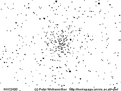
Figure 1: NGC 2420 (Image Credit: WEBDA)

For the all-sky photometry analysis, the calibrated images of NGC 2420 are utilized which are taken from the final Data Release 12 (DR12) of the SDSS-III (https://dr12.sdss.org/). In order to perform photometry on all the 192 stars, five images at different RA and DEC are selected under each g, r, and i band. Further, the ’tsfield’ file for the respective five set of images at different celestial coordinates are taken to extract the parameters for the calibration of magnitudes and also for determining the corresponding magnitude errors. The SDSS archive has images taken from 2.5-m f/5 modified Ritchey-Chrétien altitude-azimuth telescope located at Apache Point Observatory, in south east New Mexico. The five images of the NGC 2420 in g band having angular size of 10and the exposure time of 53.907 sec are presented in Fig.  2.

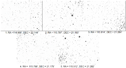
Figure 2: g band images of NGC 2420 at different RA and DEC

2. Aperture Photometry

The concept of stellar magnitudes was first brought in by the Greek astronomer Hipparchus in B.C 130. He classified stars based on their visual brightness (here on wards Magnitude) on a scale that ranged from 1 to 6. According to his classification system, the brightest starts fall under first class while stars with least brightness corresponds to the sixth category. With the advent of telescope and with the realization that the human eye has a logarithmic response to light, new magnitude scale has been introduced by Norman Pogson. In this system, over an increasing magnitude scale, any particular star is 100 times brighter than its sixth higher magnitude star [Budding, E. et al., 2007].

The photometry involves measurement of a stars’ brightness in form of magnitude from the digital image. When an image of a star is taken then that image would not only have light from the star but it also includes the light from the background sky. This causes the light from a star to spread into wider area. Thus, it is essential to distinguish starlight from the background sky light. This could be done in different ways, of which one of the most popular technique being aperture photometry. It should also to be noted that prior to measuring the magnitudes from the images various instrumental effects should be removed from them. Some of the image calibrations requirements are de-biasing, flat-fielding, and removal of the bad pixels effects and cosmic-ray events [Palmer, J. et al., 2001].

In aperture photometry, pixels that contain starlight are covered by a small circular patch known as aperture. The background sky light is then captured by a doughnut shaped patch, also named as annulus, whose center radius is larger than that of the star aperture. Fig.  3(a) shows the star aperture and the sky annulus. The light from the background sky is then eliminated by subtracting pixels in background sky annulus from the star aperture [Berry, R. et al., 2000, Beck, S.J. et al, 2014]. The best way to select appropriate star radius is to first find the full width half maximum (FWHM) of the star brightness curve or find its Gaussian sigma ($\sigma$). Then the radius of star aperture is selected as $\sigma$ or half of the FWHM value. However, to capture the starlight in totality the best practice is to set star radius five times the $\sigma$ radius. Whereas, the inner radius of the background sky aperture should be set at least twice that of the star aperture. This would prevent the inclusion of any starlight into the sky annulus. The Fig.  3(b) depicts the brightness profile of a star located at RA = 114.346°and DEC = 21.676°in NGC 2420 which is obtained through Makali’i software. The FWHM and $\sigma$ are related by the Eq. (1).

$$FWHM = 2.37\sigma$$ (1)

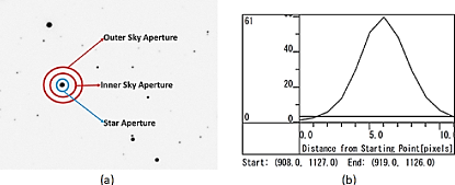
Figure 3: (a) Star aperture and sky annulus, and (b) Brightness profile of a star located at RA = 114.346°and DEC = 21.676°in NGC 2420 obtained through Makali’i software

Once the photometric observations are achieved, they could be fitted to the theoretical isochrones to determine the essential stellar parameters such as metallicity, stellar reddening, distance and ages. The isochrones are the mathematical models which represents the Hertzsprung–Russell (HR) diagram for a particular metallicity and age [Fatima, H. et al., 2016]. For instance, the surface temperature of an object could be determined by fitting the color-magnitude diagram (CMD) with the HR diagram. Thus, different isochrones are overlapped with the photometric observations and the best fit isochrones are selected for the determination of the above mentioned parameters. The database for isochrones could be found at the website of Padova database (http://pleiadi.pd.astro.it/).

The magnitude of a star is obtained by accessing the pixel values present in the star aperture and the sky annulus. These pixel values are also known as “pixel count” and the magnitude obtained from these pixel counts is known as “instrumental magnitude”. There are various ways to obtain instrumental magnitude from the star aperture counts and the background sky aperture count [Berry, R. et al., 2000, Palmer, J. et al., 2001]. One of the relationships between them is shown in Eq. (2) [Berry, R. et al., 2000]:

$$m_{ins} = -2.5\left(\frac{C_{apt}-n_{apt}\left(\frac{C_{apt}}{n_{ann}}\right)}{t}\right)+\Lambda$$ (2)

In the relation (2), the $C_{apt}$ and $n_{apt}$ are the sum of pixel values and number of pixels in the star aperture, respectively, $n_{ann}$ is the number of pixels in the background sky annulus, and $\Lambda$ is an arbitrary constant. The arbitrary constant, $\Lambda$, is added to the instrumental magnitudes so that color difference becomes equal to zero [Berry, R. et al., 2000, Palmer, J. et al., 2001].

2.1. Differential Aperture Photometry

In the differential aperture photometry, the apparent magnitude of the target star is obtained from the instrumental magnitude by comparing the target star with the standard star (also known as comparison star) that is present in the same field of view (FOV). In this technique, the target star has the same FOV, same observation time, also it is observed through same filter and same atmosphere as that of the standard star. Hence, all the atmospheric and equipment parameters affecting the brightness are cancelled out when the difference between the standard and target star is taken. The only significant parameter to be taken into account is the difference of the target and the standard star. The apparent magnitude of the target star in this case is obtained by the Eq. (3) [Warner, B.D., 2006].

$$M_{t} = \left(m_{ins\_t}-m_{c}\right)+M_{c}$$ (3)

In the Eq. (3), $M_{t}$ and $m_{ins\_t}$ are the apparent and instrumental magnitude of the target star, respectively, while the standard and the instrumental magnitude of the standard (comparison) star is represented by $M_{c}$ and $m_{c}$, respectively. The selection of standard star is crucial while performing the differential photometry as the magnitude obtained here is solely dependent on the difference of the standard and target star. Thus, the standard star magnitude should be accurately determined in this technique. The points that should be taken care of while selecting the standard star for comparison are as follows [Beck, S.J. et al, 2014, Palmer, J. et al., 2001]:

1. It should be a non-variable star.

2. It should not be a saturated star

3. It should lie near to the target star but not near any edges of the image.

4. It should be a discrete star not blended with other star/s.

5. All the comparison stars should have similar wavelength (color).

6. It should not be a very blue or very red star.

7. It should have at least 100 signal-to-noise ratio (SNR) value.

8. It should have the magnitude near to the target star so that the magnitude error is similar.

Herein, the Makali’i software is utilized to obtain the star count and the background sky count pixels values for the determination of instrumental magnitude. Makali’i software provides the “Result count” by a single click on the image (g, r, and i images of the NGC 2420 in FITS file format) at the location of the target/comparison star. The results generated on the software could be stored as CSV file format which is then used to obtain the magnitude of the target and the standard stars. The instrumental magnitude is obtained by substituting ”Result count” in the Eq. (4). Then to this instrumental magnitude, the standard magnitude value of the comparison star (obtained from the catalog) and its pixel count are added (Ref. Eq. (6)) to obtain the apparent magnitude.

$$m = -2.5\log_{10}{(count)}$$ (4)

$$m_{target}-m_{comp} = -2.5\log_{10}{\left(count_{target}\right)}-\left(-2.5log_{10}{(count_{comp})}\right)$$ (5)

$$m_{target} = -2.5log_{10}{\left(\frac{count_{target}}{count_{comp}}\right)}+m_{comp}$$ (6)

Although, the differential photometry is easy but to determine the magnitude of any target star, the standard magnitude of the comparison star should be known beforehand. Also, the comparison star should be on the same FOV as that of the target star. If the comparison star is located out of the FOV then the magnitude is obtained by the all-sky aperture photometry technique. The differential photometry is employed, in general, when it is required to investigate any change in the ”target” over certain interval of time. In this technique, accuracy of the apparent magnitude depends on the selection of the comparison star and on the exactness of the target and comparison star difference.

2.2. All-Sky Aperture Photometry

All-sky photometry provides the magnitude of the target directly from the images taken at known atmosphere and system from a set of standard stars. This technique is applied when the standard stars are outside the FOV, when the images are taken at different time, through different filters and atmosphere. Hence, the all-sky photometry requires meticulous observations that are subjected to thorough and careful data reductions. This section presents the procedures, in-detail, to obtain the values for the calibration parameters, viz., atmospheric extinction-coefficient, air-mass, zero point, color term and color index. In addition, the steps to calculate the error magnitude is presented.

The procedure to find the instrumental magnitude of the star in this technique is similar to that of the differential photometry. The formula for determining the instrumental magnitude is defined by the Eq. (7).

$$m_{ins} = -2.5\log_{10}{(count_{target})}+\Lambda$$ (7)

Eventually, the instrumental magnitude is converted into calibrated magnitude. The calibrated magnitude takes into account of effects of atmospheric extinction coefficient (k), air-mass(X), color correction term (C), and color index (CI), to determine a magnitude which is tied to the standard photometric system [Bessell, M.S., 2005]. The calibrated magnitude is defined by the Eq. (8) [Berry, R. et al., 2000, Warner, B.D., 2006, Gallaway, M., 2016, Palmer, J. et al., 2001].

$$M=m_{ins}-\Lambda+ZP+kX+C\times CI$$ (8)

The following section presents the steps to obtain the values of the above mentioned calibration parameters [Berry, R. et al., 2000, Warner, B.D., 2006, Gallaway, M., 2016, Palmer, J. et al., 2001] from the observed images.

0.0.1 2.2.1 Air-mass(X):

Air-mass is known as the length of the air-path which starlight travels through. As the light travels through some distance of the atmosphere, some fixed portion of light gets attenuated. Thus, it is necessary to find out what amount of light is lossed due to a particular unit of the air-mass. The air-mass (length of air-path) depends solely on the zenith distance, $z_{L}$. The zenith distance is obtained from the Eq. (9) [Palmer, J. et al., 2001].

$$X=sec(z_{L}) = \frac{1}{(sin\phi)(sin\delta)+(cos\phi)(cos\delta)(cosh)}$$ (9)

In the above relationship, $\phi$ is the latitude of observation, $\delta$ and $h$ are the Declination and the hour angle of the observed target, respectively. The Right Ascension ($\alpha$) of the observed target and the local sidereal time ($s$) are related to the hour angle by the Eq. (10).

$$h = s-\alpha$$ (10)

0.0.2 2.2.2 Atmospheric Extinction Coefficient (k):

The atmospheric extinction is defined as the dimming of a starlight as it passes through the atmosphere. It has the units of magnitudes/air-mass. As the air-path increases, the extinction also increases.

There are various methods to attain extinction coefficient. One of the widely used method to determine the atmospheric extinction is to observe the same non-variable star during the night with any of the suitable filter at various intervals as well as at different zenith angles. The observed magnitude of the observed star is then plotted against the calculated air-mass. The graph thus, plotted should have a straight line where the slope is equal to the extinction. The atmospheric extinction depends strongly on the wavelength. For instance, extinction is lower for red band than for the blue. Thus, in order to neutralize the extinction precisely, the color of the star has to be included. The extinction is then represented by the Eq. (11).

$$k = k^{{}^{\prime}}-k^{{}^{\prime\prime}}(CI)$$ (11)

$k^{{}^{\prime}}$ is the first order extinction in the particular color filter, $k^{{}^{\prime\prime}}$ is the second order extinction for that filter, CI is the standard color index. $k^{{}^{\prime\prime}}$ has the units of magnitudes/air-mass /magnitude of CI. Theoretically, $k^{{}^{\prime\prime}}$ is 0 for the V filter and for the following CI: U–B and B–V. Practically, the value of $k^{{}^{\prime\prime}}$ is very small and is hard to measure, hence it is ignored. However, to find $k^{{}^{\prime\prime}}$, one could refer [Warner, B.D., 2006]. The magnitude after the compensation of extinction is represented with a suffix ‘o’, it indicates that extinction effects have been removed from the magnitude. Sometimes, this magnitude is also known as exoatmospheric magnitude and is represented by the Eq.(12)

$$m_{o} = m-k^{{}^{\prime}}X-k^{{}^{\prime\prime}}X(CI)$$ (12)

0.0.3 2.2.3 Color Index (CI) and Color-Correction Term (C):

The system response for a particular band of color filter may not be identical to that of the standard photometric system. Thus, the color index and color correction terms are included to remove any color dependency. The color term is determined by obtaining the difference of the adjacent color filter band. For instance, B-V, V-R, g-r, and r-i, to name a few. The change in the response between the system under consideration and the standard photometric system is linear for a particular color band (Ref. Fig.  5). Hence, the color correction term is obtained in a manner similar to that applied for obtaining $k$. That is, observing the star for certain interval of time throughout the night at different $z_{L}$ and then the best values for $k$ and $C$ are determined by fitting the Eq. (13) using the method of least square.

$$M = m_{ins}-\Lambda+kX+C\times{CI}$$ (13)

0.0.4 2.2.4 Zero Point (ZP):

Eventually, the exoatmospheric magnitude obtained from the above calibration process is transformed to a magnitude that is tied to a standard photometric system. For the determination of the zero point it is essential to observe a primary or secondary standard star. The zero point is determined from the exoatmospheric standard star magnitude. The zero point magnitude is then calculated from Eq(14).

$$m_{zp} = m_{std}-m_{ostd}$$ (14)

In the above equation, $m_{zp}$ is the zero-point magnitude, $m_{std}$ is the catalog standard magnitude and $m_{ostd}$ is the exoatmosphric instrumental magnitude of the standard star.

2.3. Error Magnitude

Because of the Poisson statistic behaviour of the detected photon there is a inherent error in the photometry magnitude. The two ways to represent this error or uncertainty are the signal-to-noise ratio and the standard deviation present in the calculated magnitude of the star. The magnitude error, $\sigma_{m}$, for a star is defined by the Eq(15). This formula determines that if $S/N$ is $x$, then there is $x\%$ of error in the measured magnitude [Berry, R. et al., 2000, Howell, S.B., 2000].

$$\sigma_{m} = \frac{1.086}{S/N}$$ (15)

There is single signal source while there are several sources of noise such as noises from the sky as well as noises from the detector. The noise sources taken into account are readout noise, dark current, quantization noise, noise due to star background count, to name a few. The signal-to-noise ratio is thus defined by the Eq. (15) [Howell, S.B., 2000].

$$\frac{S}{N} = \frac{N_{*}}{\sqrt{N_{*}+n_{pix}(N_{S}+N_{D}+N_{R}^{2})}}$$ (16)

The numerator in the above equation, $N_{\**}$, is the total number of photons detected from the target. The terms in denominator of the Eq(16) are defined as $n_{pix}$ is the number of pixels present in the target, $N_{S}$ is the total number of photons per pixel from the background sky, $N_{D}$ is the total number of dark current electrons per pixel, and $N_{R}^{2}$ is the total number of electrons per pixel resulting from the readout noise. The further details on the magnitude error could be found in [Howell, S.B., 2000].

3. WORK DESCRIPTION

The all-sky photometry is performed on the 192 stars lying within and near the radius of 6from the center of NGC 2420. The stars are selected on the basis of brightness perceived through naked eyes. The selected region and the star numbers are adopted from [Cannon, R.D. et al., 1970]. As mentioned in Section 1, five different images are extracted for each g, r, and i bands to cover all the 192 stars. The combined g band image with the selected 192 stars is presented in Fig.  4 (North up and East left) and their celestial coordinates are presented in Table 1. Each of these fifteen images are then analyzed through Makali’i software to convert the raw counts of the selected stars into the raw instrumental magnitudes. As the NGC 2420 is an old open cluster, hence the values for air-mass ($X$), atmospheric extinction ($k$), and zero points ($ZP$) are obtained from the ’tsfield’ file present in the SDSS archive. The values of these calibration parameters are depicted in Table 2.

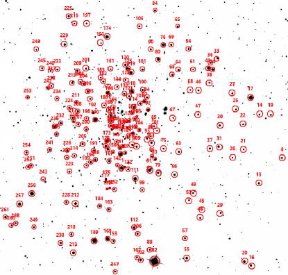
Figure 4: g-band image of NGC 2420 with the 192 selected stars

Table 1: Celestial coordinates of the 192 selected stars in NGC 2420

Star No.	RA(°)	DEC(°)	Star No.	RA(°)	DEC(°)	Star No.	RA(°)	DEC(°)	Star No.	RA(°)	DEC(°)
8	114.464	21.544	84	114.572	21.661	138	114.600	21.567	199	114.630	21.539
10	114.473	21.579	85	114.572	21.569	140	114.601	21.548	200	114.630	21.568
13	114.483	21.524	86	114.574	21.546	141	114.601	21.553	201	114.630	21.615
14	114.483	21.578	87	114.574	21.556	142	114.603	21.539	204	114.632	21.603
16	114.490	21.459	88	114.575	21.561	143	114.603	21.564	205	114.633	21.556
17	114.490	21.592	89	114.575	21.473	144	114.604	21.601	206	114.635	21.604
20	114.495	21.463	90	114.575	21.630	145	114.604	21.557	207	114.637	21.572
21	114.497	21.551	91	114.576	21.535	146	114.604	21.569	208	114.637	21.582
22	114.497	21.571	92	114.577	21.583	147	114.605	21.455	209	114.638	21.613
25	114.503	21.583	93	114.578	21.560	149	114.605	21.563	211	114.639	21.589
26	114.506	21.545	94	114.578	21.593	152	114.605	21.520	212	114.639	21.509
27	114.506	21.595	97	114.580	21.589	153	114.606	21.479	213	114.640	21.470
28	114.507	21.480	99	114.582	21.519	155	114.607	21.585	214	114.640	21.547
29	114.515	21.500	100	114.582	21.598	156	114.608	21.550	215	114.640	21.650
30	114.517	21.570	101	114.582	21.614	157	114.608	21.568	216	114.641	21.574
31	114.518	21.554	102	114.583	21.464	158	114.608	21.574	217	114.642	21.577
33	114.519	21.623	103	114.584	21.588	159	114.609	21.578	218	114.642	21.484
34	114.523	21.614	104	114.585	21.567	160	114.609	21.570	219	114.642	21.604
36	114.524	21.619	105	114.585	21.648	161	114.609	21.615	223	114.644	21.534
37	114.525	21.552	106	114.586	21.485	162	114.609	21.521	224	114.644	21.585
38	114.526	21.603	107	114.587	21.467	163	114.610	21.504	225	114.645	21.656
40	114.526	21.623	108	114.587	21.577	164	114.610	21.594	226	114.646	21.552
41	114.526	21.615	109	114.587	21.553	166	114.611	21.583	227	114.646	21.545
45	114.533	21.496	110	114.588	21.569	167	114.611	21.543	228	114.647	21.510
46	114.535	21.598	111	114.588	21.528	169	114.611	21.480	229	114.648	21.634
47	114.535	21.578	112	114.589	21.490	170	114.611	21.520	230	114.651	21.478
48	114.535	21.493	113	114.589	21.576	171	114.612	21.552	232	114.652	21.573
49	114.539	21.516	114	114.590	21.585	172	114.612	21.596	233	114.654	21.615
51	114.540	21.614	115	114.590	21.564	173	114.612	21.558	234	114.655	21.592
53	114.542	21.511	116	114.590	21.555	174	114.613	21.640	235	114.655	21.564
54	114.541	21.633	117	114.590	21.580	175	114.612	21.528	236	114.657	21.570
55	114.544	21.466	118	114.592	21.598	176	114.613	21.554	237	114.659	21.608
57	114.546	21.481	119	114.592	21.612	177	114.613	21.526	238	114.660	21.602
58	114.547	21.596	120	114.593	21.563	180	114.615	21.586	240	114.660	21.613
63	114.551	21.549	121	114.594	21.593	182	114.616	21.605	241	114.661	21.551
64	114.552	21.614	122	114.593	21.535	183	114.617	21.608	242	114.663	21.600
65	114.552	21.648	123	114.594	21.574	184	114.618	21.507	245	114.667	21.615
66	114.555	21.531	124	114.595	21.561	188	114.622	21.544	248	114.672	21.630
67	114.556	21.576	125	114.595	21.615	189	114.622	21.479	249	114.674	21.491
68	114.557	21.610	126	114.595	21.568	190	114.622	21.575	250	114.676	21.517
69	114.558	21.634	127	114.596	21.538	191	114.624	21.551	251	114.676	21.539
75	114.564	21.552	128	114.597	21.606	192	114.625	21.581	252	114.679	21.538
76	114.564	21.634	129	114.597	21.549	193	114.618	21.635	253	114.680	21.593
79	114.568	21.533	130	114.597	21.618	194	114.626	21.542	254	114.680	21.549
80	114.569	21.623	132	114.598	21.595	195	114.627	21.591	257	114.686	21.509
81	114.570	21.566	133	114.598	21.570	196	114.629	21.597	258	114.689	21.494
82	114.571	21.463	134	114.599	21.568	197	114.650	21.650	260	114.693	21.492
83	114.571	21.543	135	114.599	21.554	198	114.630	21.576	261	114.698	21.499

Table 2: Calibration parameters obtained from the ’tsfield’ files of the respective five different set of images

Set of Images	air mass	Zero Point	Extinction Factor
1	1.2068	23.818	0.414
2	1.1815	23.507	0.4176
3	1.1805	23.507	0.4176
4	1.0657	23.521	0.4467
5	1.0651	23.526	0.4467

The final calibrated magnitudes and the magnitude errors for the selected stars in g, r, and i bands are obtained by substituting the values of the calibration parameters from the Table 2 into the relations described in Section 2.2 and Section 2.3, respectively. The excel spreadsheets are utilized for finding out the results from the respective equations. The SAOImage DS9 [Joye, W. et al., 2020] software is used to locate and assign numbers to the selected stars. The calculated calibrated magnitudes and error magnitudes for the first 30 stars are depicted in Table 3, which are also compared with their respective catalog values. The SDSS DR12 catalog [SDSS catalog] is referred for comparing the calculated results.

Table 3: Calculated calibrated magnitudes and error magnitudes for the first 30 stars in g, r, and i bands

Stars	Calculated Calibrated Magnitudes			Calculated Magnitude Error			Catalog Magnitudes			Catalog Magnitudes Errors
	g	r	i	e_g	e_r	e_i	g	r	i	e_g	e_r	e_i
8	13.695	13.823	14.070	0.0014	0.0015	0.0016	14.866	14.653	14.608	0.003	0.004	0.004
10	14.408	14.422	14.617	0.0019	0.0019	0.0021	15.566	15.245	15.143	0.003	0.004	0.004
13	13.437	13.261	14.128	0.0012	0.0011	0.0017	14.663	14.206	14.241	0.003	0.008	0.005
14	14.165	14.066	14.217	0.0017	0.0016	0.0017	15.332	14.902	14.747	0.003	0.004	0.004
16	13.147	13.277	13.943	0.0011	0.0011	0.0016	14.362	14.162	13.27	0.003	0.004	0.003
17	12.444	12.842	13.568	0.0008	0.0009	0.0013	11.787	11.654	11.686	0.001	0.001	0.001
20	13.355	13.416	14.282	0.0012	0.0012	0.0018	15.024	14.751	14.973	0.01	0.011	0.012
21	14.189	14.202	14.406	0.0017	0.0017	0.0019	15.36	15.049	14.934	0.003	0.004	0.004
22	14.361	13.936	13.963	0.0019	0.0015	0.0016	15.52	14.761	14.475	0.003	0.004	0.004
25	13.990	13.819	13.935	0.0016	0.0014	0.0015	15.159	14.651	14.462	0.003	0.004	0.004
26	14.472	14.380	14.533	0.0020	0.0019	0.0020	15.643	15.205	15.054	0.003	0.004	0.004
27	13.462	13.552	13.785	0.0012	0.0013	0.0014	14.631	14.388	14.315	0.003	0.004	0.004
28	14.333	14.441	14.685	0.0019	0.0020	0.0022	15.541	15.316	15.259	0.003	0.004	0.004
29	13.528	13.256	14.010	0.0013	0.0011	0.0016	14.744	14.215	14.177	0.003	0.008	0.005
30	13.105	13.035	13.983	0.0010	0.0010	0.0016	14.373	13.964	13.959	0.003	0.006	0.004
31	13.639	13.675	13.877	0.0013	0.0014	0.0015	14.803	14.508	14.396	0.003	0.004	0.004
33	13.466	13.549	13.787	0.0012	0.0013	0.0014	14.63	14.384	14.316	0.003	0.004	0.004
34	12.860	13.217	13.600	0.0009	0.0011	0.0013	15.438	15.319	14.789	0.012	0.012	0.012
36	13.833	13.958	14.213	0.0015	0.0015	0.0017	15.003	14.793	14.738	0.003	0.004	0.004
37	13.546	13.226	13.934	0.0013	0.0011	0.0015	14.809	14.707	15.601	0.003	0.011	0.013
38	14.063	14.136	14.358	0.0016	0.0017	0.0019	15.235	14.965	14.884	0.003	0.004	0.004
40	14.541	14.621	14.846	0.0020	0.0021	0.0024	15.714	15.458	15.374	0.004	0.004	0.004
41	12.813	13.103	13.479	0.0009	0.0010	0.0012	15.507	14.945	14.756	0.012	0.011	0.012
45	15.494	15.455	15.619	0.0032	0.0032	0.0035	16.649	16.257	16.134	0.004	0.004	0.005
46	14.287	14.358	14.590	0.0018	0.0019	0.0021	15.451	15.195	15.114	0.003	0.004	0.004
47	14.384	14.461	14.696	0.0019	0.0020	0.0022
48	14.117	14.256	14.488	0.0017	0.0018	0.0020	15.278	15.07	15.017	0.003	0.004	0.004
49	13.839	13.966	14.211	0.0015	0.0016	0.0017	14.99	14.775	14.719	0.003	0.004	0.004
51	14.512	14.469	14.646	0.0020	0.0020	0.0021	15.669	15.307	15.166	0.004	0.004	0.004
53	14.025	13.328	14.267	0.0016	0.0012	0.0018	15.175	14.145	14.22	0.003	0.004	0.002

Further, these g, r, and i magnitudes are the transformed into the B, V, and R band magnitudes of Johnson-Cousins UBVRI standard photometric system by using transform equations: Eqs. (17) to (19) [Lupton, R., 2005]. The calculated B, V, and R, magnitudes are presented in the Table 4. These calculated B, V, and R magnitudes are compared with the NOMAD-1 catalog magnitudes [NOMAD-1 catalog]. Also, the color magnitude diagram (CMD) prepared from the calculated calibrated magnitudes of the 192 selected stars for both the standard photometry systems are presented in Fig.  5.

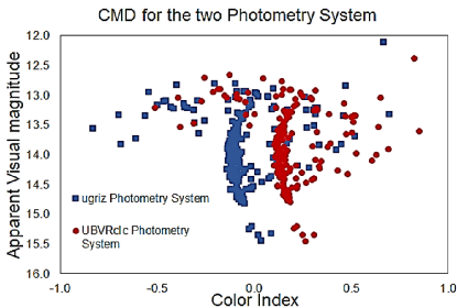
Figure 5: The color magnitude diagram for the $ugriz$ and $UBVR_{c}I_{c}$ standard photometry system

$$B = g_{cal}+0.3130\times{(g_{cal}-r_{cal})}+0.2271$$ (17)

$$V = g_{cal}-0.5784\times{(g_{cal}-r_{cal})}-0.0038$$ (18)

$$R = r_{cal}-0.2936\times{(r_{cal}-i_{cal})}-0.1439$$ (19)

Table 4: Transformed B, V, and R magnitudes

Stars	Calculated Calibrated Magnitudes			Catalog Magnitudes			Stars	Calculated Calibrated Magnitudes			Catalog Magnitude
	B	V	R	B	V	R		B	V	R	B	V	R
8	13.882	13.766	13.752	14.44	14.54	14.39	31	13.855	13.656	13.590	14.23	14.50	13.99
10	14.631	14.412	14.335	15.86	17.97	14.90	33	13.667	13.510	13.475	14.23	14.41	14.10
13	13.720	13.332	13.372	14.30	14.22	13.78	34	12.976	13.063	13.186	13.46	17.97	11.77
14	14.424	14.104	13.966	14.71	15.29	14.28	36	14.021	13.901	13.889	15.19	14.78	14.75
16	13.334	13.219	13.329	14.09	14.08	13.99	37	13.873	13.357	13.290	14.52	14.21	13.90
17	12.547	12.671	12.911	12.02	11.38	10.95	38	14.267	14.101	14.057	14.54	14.85	14.71
20	13.563	13.387	13.527	16.37	17.78	13.06	40	14.743	14.584	14.543	15.02	14.62	15.33
21	14.412	14.193	14.118	15.14	15.02	14.90	41	12.949	12.977	13.070	15.22	15.05	15.01
22	14.721	14.112	13.800	15.13	14.89	13.83	45	15.734	15.468	15.359	16.27	15.99	16.35
25	14.270	13.887	13.709	14.78	14.62	14.40	46	14.492	14.324	14.282	15.22	15.05	15.01
26	14.727	14.415	14.281	15.31	15.21	15.10	47	14.587	14.425	14.386	15.23	15.22	15.07
27	13.661	13.510	13.476	14.23	14.30	14.21	48	14.300	14.194	14.180	14.65	14.71	15.06
28	14.526	14.392	14.369	15.17	15.27	15.18	49	14.026	13.909	13.894	14.44	14.86	14.22
29	13.840	13.367	13.333	14.39	14.17	13.55	51	14.752	14.483	14.377	15.29	14.96	15.01
30	13.354	13.060	13.169	13.99	13.94	13.73	53	14.470	13.618	13.460	15.10	14.42	13.93

It is observed that there is certain deviation between the calculated and standard magnitudes. This is due to the accuracy with which the software counts the star minus background sky counts, accuracy of detecting the aperture center and the aperture parameters set while performing the aperture photometric analysis through Makali’i software. In addition, it is noted that the Makali’i softwar is capable of providing best results for the bright stars only. It is analyzed that the Makali’i software is effective for the stars which have star minus background sky count value of 500 or greater. For the validation of this statement, some of the dim stars are considered whose celestial coordinates are presented in Table 5. In this analysis, the star celestial coordinates and their respective numbers are adopted from [Ciroi, S. et al., 2009, Rafanelli, P., et al. 2011]. The reason for selecting these stars is that most of these are the dim stars in the g-band and are good candidates for dim star analysis by Makali’i software. On analyzing the g-band images, it is observed that some dim stars have the result counts below 500 and for some stars the result counts are even zero. For these star the instrumental magnitude would not be accurate. Hence, it could be said that although the Makali’i software is simple and user friendly software but it is unable to detect and provide results counts for very faint stars. This software provides effective output for the bright stars.

Table 5: Celestial coordinates for the analysis of dim stars in the g-band images of NGC 2420

Undetectable Stars			Stars having Result Count less than 500
Star No.	RA(°)	DEC(°)	Star No.	RA(°)	DEC(°)
II	114.651	21.486	XV	114.834	21.335
III	114.654	21.529	XVI	114.811	21.427
V	114.492	21.529	XVII	114.821	21.546
VI	114.501	21.452	XX	114.694	21.496
VII	114.353	21.243	XXIII	114.382	21.230
IX	114.393	21.279	XXV	114.214	21.695
X	114.361	21.547	XXVI	114.374	21.682
XIV	114.792	21.636	XXVII	114.681	21.967
XXI	114.502	21.350	XXVIII	114.674	21.947
XXII	114.535	21.444	XXIX	114.751	21.612
XXIV	114.331	21.473

Conclusion

This article provides the insight into the physics of differential and all-sky aperture photometry by manually scanning the astronomical images. The astronomical images of NGC 2420 are analyzed through a Windows based software: Makali’i. The g, r, and i magnitudes and error magnitudes of 192 selected stars present in an old open cluster NGC 2420 is calculated and then compared with the respective standard magnitudes and error magnitudes of the catalog. It is analytically observed that the Makali’i software does effective photometry analysis for the bright stars. However, for the faint star the software is unable to obtain the photon counts. It is noted that for count value (star minus background sky) of less than 500, the instrumental magnitude is not accurate. To overcome this deviation instead of using Makali’i software one could utilize aperture photometry tool (APT). Further, all the calibration parameters required for obtaining the calibrated magnitude is described in detail which are then used to obtain the calibrated instrumental magnitude. In addition, the calibrated instrumental magnitudes are transformed into the B, V, and R band magnitudes of Johnson-Cousins UBVRI standard photometric system. Also, the color magnitude diagrams for both $ugriz$ and $UBVR_{c}I_{c}$ standard photometric systems are presented which are obtained from the calculated calibrated magnitude. Thus, this article aids the non-professionals to familiarize with the fundamentals of the differential and the all-sky aperture photometry.

Acknowledgments: The authors are grateful to Dr. Rucha Desai (Associate Professor, PDPIAS, CHARUSAT), Dr. Dipanjan Dey (Assistant Professor, ICC, CHARUSAT) and Mr. Parth Bambhaniya (Research Scholar, ICC, CHARUSAT) for their valuable suggestions in the completion of this work.

References

- [Allison, M., 2006] Allison, M., 2006, Star Clusters and How to Observe Them, Springer.
- [Anthony-Twarog, B.J. et al., 1990] Anthony-Twarog, B.J., Kaluzny, J., Shara, M.M., Twarog, B.A., 1990,The Astronomical Journal, pp.1504-1535, 99.
-
[Beck, S.J. et al, 2014]
Beck, S.J., Henden, A.A., Templeton, M.R., 2014, The AAVSO Guide to CCD Photometry, AAVSO, Cambridge, MA.
(https://www.aavso.org/sites/default/files/publications_files/ccd_photometry_guide/
CCDPhotometryGuide.pdf) - [Berry, R. et al., 2000] Berry, R., Burnell, J., 2000, The Handbook of Astronomical Image Processing, Willmann-Bell. Inc., Richmond, Virginia, USA.
- [Bessell, M.S., 2005] Bessell, M.S., 2005,Annu. Rev. Astron. Astrophys., pp.293-336, 43.
- [Budding, E. et al., 2007] Budding, E., Demircan, O., 2007, Introduction to astronomical photometry , Cambridge University Press.
- [Cannon, R.D. et al., 1970] Cannon, R.D., Lloyd, C., 1970, Monthly Notices of the Royal Astronomical Society, pp.279-297, 150.
- [Ciroi, S. et al., 2009] Ciroi, S., Di Mille, F., Rafanelli, P., 2009,Proceedings of the International Astronomical Union, 5, S260.
- [Fatima, H. et al., 2016] Fatima, H., Mushtaq, M., Rahman, S.F.U., 2016,Journal of GeoSpace Science, pp.1-13 (arXiv: 1609.02480).
- [Gallaway, M., 2016] Gallaway, M., 2016, An Introduction to Observational Astrophysics, Springer.
-
[Grisetti, R., 2006]
Grisetti, R., 2006, A Student’s Guide to CCD Photometry Data Processing using IRAF, University of Central Florida.
(http://zeus.asu.cas.cz/koci/x/ourmanual.pdf) - [Hanisch, R.J. et al., 2001] Hanisch, R.J., Farris, A., Greisen, E.W., Pence, W.D., Schlesinger, B.M., Teuben, P.J., Thompson, R.W., Warnock, A., 2001,Astronomy & Astrophysics, pp.359-380, 376, 1.
- [Horaguchi, T. et al., 2006] Horaguchi, T., Furusho, R., Agata, H., Wg, P., 2006,Astronomical Data Analysis Software and Systems, p. 544, 351.
- [Howell, S.B., 2000] Howell, S.B., 2000, Handbook of CCD Astronomy, Cambridge University Press.
- [Joye, W. et al., 2020] Joye, W., Mandel, E, Murray, S., 2020, SAOImage DS9. Vers. 8.0. 1. Computer software. Future Directions for Astronomical Image Display.
-
[Lupton, R., 2005]
Lupton, R., 2005, Transformations between SDSS magnitudes and other systems
(https://www.sdss.org/dr12/algorithms/sdssUBVRITransform/#Lupton2005) - [McClure, R.D. et al., 1974] McClure, R.D., Forrester, W.T., Gibson, J., 1974,The Astrophysical Journal, p.409, 189.
-
[NOMAD-1 catalog]
NOMAD-1 catalog (Zacharias et al. 2005)
(http://vizier.u-strasbg.fr/viz-bin/VizieR?-source=I/297&-to=3) - [Oralhan, I.A. et al., 2015] Oralhan, I.A., Karataş, Y., Schuster, W.J., Michel, R., Chavarría, C., 2015,New Astronomy, pp.195-210, 34.
- [Palmer, J. et al., 2001] Palmer, J., Davenhall, A.C., 2001, The CCD Photometric Calibration Cookbook, Starlink Cookbook.
-
[Rafanelli, P., et al. 2011]
Rafanelli, P., Ciroi, S., Cracco, V., Frassati, A., Spiga, R., 2011, The Sky as a Laboratory, Book_2012.
(http://www.astro.unipd.it/progettoeducativo/Tesine/2011-12/relazioni/book_2012
.pdf) - [Robitaille, T.P. et al., 2013] Robitaille, T.P., Tollerud, E.J., Greenfield, P., Droettboom, M., Bray, E., Aldcroft, T., Davis, M., Ginsburg, A., Price-Whelan, A.M., Kerzendorf, W.E., Conley, A., et al., 2013,Astronomy & Astrophysics, p.A33, 558.
-
[Romanishin, W., 2006]
Romanishin, W., 2006, An Introduction to Astronomical Photometry Using CCDs, University of Oklahoma.
(http://hildaandtrojanasteroids.net/wrccd22oct06.pdf) -
[SDSS catalog]
The SDSS Photometric catalog, Release 12
(http://vizier.u-strasbg.fr/viz-bin/VizieR?-source=V/147&-to=3) - [Tody, D., 1986] Tody, D., 1986,Instrumentation in Astronomy, pp. 733-748, 627.
- [Warner, B.D., 2006] Warner, B.D., 2006, A practical Guide to Lightcurve Photometry and Analysis, Springer.