Quantitative probing: Validating causal models with quantitative domain knowledge

Abstract

We present quantitative probing as a model-agnostic framework for validating causal models in the presence of quantitative domain knowledge. The method is constructed as an analogue of the train/test split in correlation-based machine learning and as an enhancement of current causal validation strategies that are consistent with the logic of scientific discovery. The effectiveness of the method is illustrated using Pearl’s sprinkler example, before a thorough simulation-based investigation is conducted. Limits of the technique are identified by studying exemplary failing scenarios, which are furthermore used to propose a list of topics for future research and improvements of the presented version of quantitative probing. The code for integrating quantitative probing into causal analysis, as well as the code for the presented simulation-based studies of the effectiveness of quantitative probing is provided in two separate open-source Python packages.

1 Introduction

The topic of causal inference has been a focus of extensive research in statistics, economics and artificial intelligence. [1, 2, 3, 4, 5, 6] In contrast to more traditional statistics, methods of causal inference allow predicting the behavior of a system not only in situations where we passively observe certain evidence, but also in situations where we actively intervene in the data generating process. Prior to the rise of causal inference, ruling out confounding in such predictions required performing costly and possibly harmful randomized controlled trials [7]. Causal inference, on the contrary, provides the methodology to infer the effect of hypothetical actions from passively collected observational data and additional assumptions, which can be encoded in graphs [1] or conditional independence statements [3]. The benefits of evaluating a wide range of possible actions without actually having to perform them are obvious in fields including medical treatment, industrial manufacturing or governmental policy design. However, in contrast to correlation-based prediction techniques, such as linear regression models, support vector machines or neural networks, which can all be validated using the well-known train/test split [8], the challenge of validating the causal models responsible for the predictions of interest is still unsolved. Without having validated the causal model, the promising perspective of predicting the behavior of a system under interventions from purely observational data is compromised by our uncertainty about the validity of the underlying model. This gap in the methodology needs to be filled, before decision makers in the above-mentioned application domains can leverage the powerful methods of causal inference, in order to complement, enhance or even replace the costly current method of randomized controlled trials. In this paper, we present quantitative probing, a novel approach for validating causal models, which applies the logic of scientific discovery [9] to the task of causal inference. Both, the code for integrating quantitative probing into causal analysis and the code for simulation-based studies of the effectiveness of quantitative probing are provided in two separate open-source Python packages [10, 11]. The article is structured as follows: Chapter 2 reviews the train/test split as the classical method for validating correlation-based statistical models, and explains why it is not possible to directly transfer the method to the field of causal models. Chapter 3 presents different approaches to the validation of causal models and discusses the limitations of the currently available validation techniques. Chapter 4 briefly clarifies the notion of a causal model and introduces causal end-to-end analysis as a model that generalizes other types of causal models. Chapter 5 synthesizes the idea of quantitative probing from the observations in the previous chapters, and relates the approach to the established method of scientific discovery. The concept is illustrated using Pearl’s well-known Sprinkler example [1] and assumptions are explicitly stated, in order to define the current scope of the quantitative probing approach. Chapter 6 provides simulation-based evidence for the effectiveness of quantitative probing as a validation technique. Special cases where the method fails to detect misspecified models are investigated in detail, in order to identify limitations and future enhancements. Chapter 7 concludes the article by summarizing the main points and proposes concrete questions for future research.

2 The role of the i.i.d. assumption in model validation

In order to gauge the difficulty of the challenge that validation poses for causal inference procedures, it is worth taking a step back and recapitulating the reasoning behind the predominant strategy for validating traditional correlation-based statistical learning methods. These methods, which encompass both classification and regression algorithms, such as linear regression, support vector machines or numerous variations of deep learning with neural networks, have one crucial assumption in common [8]: Every sample that we have observed in fitting the model, as well as every sample that we will need to feed into the final model for classification or regression, is drawn from the same distribution, and they all are drawn independently of each other. This assumption is commonly referred to as the i.i.d. assumption, which stands for independent and identically distributed. However, it is seldomly explicitly mentioned because of how deeply ingrained it is in all correlation-based thinking about machine learning. The two parts of the term i.i.d. have important consequences for how we train or validate machine learning models:

The independence assumption is the implicit foundation of the current practices for model training: If we did not assume that all samples are drawn independently from each other, the likelihood

$$p(X,Y|\theta)=\prod_{i=1}^{n}p(x_{i},y_{i}|\theta)$$ (1)

of observing samples with features $X$ and labels $Y$ for a given parameter $\theta$ would not factorize over all the samples $(x_{i},y_{i})$. The consequence would be that the commonly used error metrics, e.g. the mean squared error or mean absolute error, would lose their theoretical backing: All of them are based on summing up independently computed prediction errors of the model for each sample, which is justified precisely by the factorization property of the likelihood (or equivalently the summation property of the log-likelihood).

The assumption of identical distribution enables the use of the train/test split for model validation: If all the samples that we will ever need to classify stem from the same distribution as the observed labelled data, we can fit our model on the observed data and be confident that the obtained model will also be suitable for classifying the new incoming data. Even the thereby caused risk of overfitting, i.e. learning overly specific characteristics of the training data that fail to generalize and lead to a worse performance on new data, can be mitigated using the same distributional assumption: If we do not train the model on all the labelled data, but only on a subset of it (the training set), we can evaluate its performance on the rest of it (the test set), given that the correct labels for the test set are available to us. Additionally, we have not used the test set for model training and it is statistically identical to the new data that we will have to classify in the actual task, because it is drawn from the same distribution. Therefore, the expected value of the prediction error for any unseen sample is equal to the mean error on the test set. In summary, we can base our confidence in the predictions of the model on its performance on the test data, which is enabled precisely by the assumption of identical distribution.

If we now try to transfer these techniques to the training and validation of causal models, we will inevitably face severe problems. The observational data that we use to train our causal models can very well follow the i.i.d. assumption. The notion of using test samples from the same distribution to evaluate how well the model performs on hypothetical queries, however, is diametrically opposed to the task of causal inference: We want to predict what happens under certain interventions, and an intervention is precisely the act of changing the data generating process. A change in the data generating process, of course, generally entails a change in the distribution from which the samples are drawn. Since we are given only observational data, we need to use something other than the pure data to gauge the usefulness of our model for the task of predicting the behavior of the system under interventions.

3 State of the art

In recent years, others have already tackled the challenging question of how to validate causal models. One common approach is to accept that the model is likely to have flaws. If these can be identified and bounded, we can still use this knowledge to obtain error bounds around the estimates of the model in the spirit of a sensitivity analysis [12, 13, 14, 15] . As an example, if we are unsure about the direction of one edge in the causal graph, we can perform the identification and estimation of the target effect for both versions of the causal graph and use the difference of the resulting estimates as an uncertainty measure. A similar approach can be used for all other parts of the causal analysis, such as choosing an estimator, hyperparameters, or treatment and outcome models. These methods are easy to implement, but they depend on the specifics of creating the causal model. Another drawback is that they do not tell us how close our model is to the correct one. Quite on the contrary, they expect us to know in which ways and how far we have deviated from the true model, in order to plug these deviations into the different variants of sensitivity analysis. For complex models, it is unlikely for researchers to take care of all possible deviations, which then leads us to doubt not only our candidate model, but also the sensitivity analysis that was supposed to be the answer to these doubts.

A second stream of research [16] takes a more straightforward approach to dealing with the unknown ground truth for the behavior of the system under interventions: We take the same algorithm that is used to create our causal model, but instead of applying it to our real data, we use simulated data. If the simulation environment can also generate data for the interventional scenarios of interest, we can then compare the predictions of the model to the simulated ground truth. While the advantages of this convenient approach are obvious, it rests on several critical assumptions that are hard to verify. First, we cannot choose any simulated data at will to gauge the performance of our model on the real data. It is clear that the data generating process in the simulation scenario must be similar to the data generating process in the actual scenario of interest. However, this requires knowledge about the scenario of interest, which we might not have. If we fully understood the data generating process, then we would not have to perform a causal analysis in the first place. A second problem is that we are not directly evaluating the performance of a model that we want to use for the real task, but we are evaluating the performance of a different model that is trained on the simulated data. The two models of interest are linked by the algorithm that is used to create them, but it is not clear to which extent the performance of one model will transfer to the performance of the other via this link.

A third approach [17] tries to employ refutation tests to probe candidate models. These tests serve as a filter to refute implausible models. An example would be to replace the data for the treatment or outcome variable by random data, which is independent of all other variables. If the model predicts a non-zero causal effect, it should clearly be refuted. Other tests include the synthetic addition of random and unobserved common causes, as well as replacing the original dataset by a subset or a bootstrapped version of itself. The idea of such checks is well in line with the scientific method [9]: A scientific theory cannot be proven, but only be falsified. If all our falsification attempts fail, the theory gains credibility. In the same sense, we have no means of directly proving our causal model right, so we try proving it wrong by the refutation tests. A drawback of the method is that these generic tests might be too weak a filter for distinguishing the correct model from plausible, but incorrect models. It is our goal to establish quantitative probing as a general validation framework that provides more powerful problem-specific refutation tests.

4 Types of causal models

In order to formulate and evaluate validation strategies for causal models, we need to specify more clearly what is meant by a causal model. In the context of validating correlation-based models, the model can be seen as a black box that answers certain queries. In the classification setting, the query could be: "Given that we have observed the following features, what class does the sample belong to?" Similarly, in the regression setting, we can ask the model: "Given that we have observed the following features, what is the value of the target variable for this sample?" Note that the above-presented train/test split strategy for validating these models does not require any knowledge about what is happening inside of the black box. We only need to be able to answer the queries for the samples in our test set, which makes the strategy applicable to a wide range of classification and regression models. Following this observation, a strategy for evaluating causal models should also be applicable to many different variants of causal analysis strategies, regardless of their implementation details. Therefore, we will use a very general definition of a causal model: We call everything a causal model that answers interventional queries, i.e. that estimates probabilities of the form $p(y|do(x=v))$ to calculate the average treatment effect (ATE)

$$\tau=p(y=1|do(x=1))-p(y=1|do(x=0))$$ (2)

from observational data. For the remainder of the article, we will restrict our studies to these ATEs in the binary data setting. Extensions to other types of causal effects, such as conditional average treatment effects [18], natural direct effects and natural indirect effects [1] are possible, but not necessary to illustrate the central ideas of our validation strategy. In the same spirit, we refrain from leaving the binary data setting, although all the arguments readily transfer to more general discrete, categorical and continuous datasets.

The considered causal model could be

• A fully parameterized causal Bayesian network [1, 19], i.e. a causal graph together with a conditional probability distribution (CPD) over each of the $n$ nodes $x_{i}$, given its respective parents $\Pi_{i}$ in the causal graph: For a given target effect, we set the treatment variable to a fixed value $v$ and multiply the CPDs

  $$p(x_{i}|\Pi_{i}=\pi_{i})$$ (3)

  of the non-treatment nodes with the delta distribution for the treatment node $x_{t}$, in order to obtain the resulting interventional distribution

  $$p(x_{1}=v_{1},...,x_{n}=v_{n}|do(x_{t}=v))=\begin{cases}\prod_{i\neq t}p(x_{i}=v_{i}|\Pi_{i}=\pi_{i})&\text{if }v_{t}=v\\ 0&\text{else.}\end{cases}$$ (4)

  The interventional mean over the outcome variable under the given treatment can then be obtained by a marginalization of the interventional distribution.

• The combination of a causal graph, Pearl’s do-calculus [1], observational data and a fixed estimation strategy: The do-calculus allows us to recover an unbiased statistical estimand for any interventional mean from the causal graph. This estimand is built purely from do-free expressions, such as ordinary conditional probabilities, which can subsequently be estimated from the observational data using the fixed estimation strategy.

• The combination of qualitative domain knowledge, a causal discovery algorithm [20, 21], Pearl’s do-calculus, observational data and a fixed estimation strategy: The procedure is the same as for method b), except we first need to use the causal discovery algorithm to recover the causal graph from our qualitative domain knowledge and the observational data.

• Any model that does not rely on graphs for the encoding of qualitative domain knowledge, e.g. a model that is based on the potential outcomes framework [3]. Due to our limited experience with these models, we will focus on graph-based causal models for the remainder of the article. However, as long as the model can answer multiple causal queries, it is suitable for validation by quantitative probing.

The enumeration shows that causal inference can be a complex pipeline of multiple analysis steps. Model b) is clearly a special case of model c), where we assume an omniscient causal discovery algorithm. In the same vein, model a) is a special case of model b), where we fit the CPDs from our observational data, assuming that we know the functional form of each CPD. Applying the do-calculus is no more necessary if the CPDs are available. In order to consider a general scenario without any restrictive assumptions about the underlying data generating process, we introduce the following graph-based causal model type that covers many simpler types of causal analysis as special cases.

By causal end-to-end analysis, we mean the following procedure for a given dataset and a given target effect.

• We preprocess the data by deleting, adding, rescaling or combining variables.

• We pass qualitative domain knowledge by specifying which edges must or must not be part of the causal graph.

• We run a causal discovery algorithm that respects the qualitative domain knowledge.

• We postprocess the proposed causal graph by deleting, adding, reversing or orienting a subset of edges in the causal discovery result.

• We identify an unbiased statistical estimand for the target effect and validation effects by applying the do-calculus to the causal graph.

• We estimate the estimands by a method of our choice.

5 Quantitative probing

Validation strategies often assume that we want to predict a single target (causal) effect, once the causal graph has been specified. We will refer to both the treatment variable and outcome variable of the target causal effect as target variables for ease of notation. All the other variables in the dataset, which we will call non-target variables, usually are either ignored or treated as confounders, based on the structure of the causal graph. In either case, they are taken care of by methods like do-calculus and we do not have to inspect their quantitative causal relationships with any of the target or non-target variables. However, not taking into account these non-target effects means wasting our domain knowledge: Just as we can pass parts of the causal graph to a causal discovery algorithm as a form of qualitative domain knowledge, we can use our expectations about selected non-target effects as supplementary quantitative domain knowledge. Analogously to communicating that we expect an edge between two variables in the causal graph, we can specifiy that we expect a certain non-target effect to be close to a given value. There is a key difference between passing qualitative and quantitative domain knowledge. The qualitative domain knowledge can be explicitly accepted as an input by a causal discovery algorithm, meaning that the procedure actively uses the knowledge in recovering the correct causal graph from the observational data [22]. For quantitative knowledge, on the other hand, it is not even clear where to pass these desiderata about the causal model and its predictions. Should we pass them to the estimation procedure and use them for hyperparameter tuning? Or could it be that the hyperparameters are correct, even when the model fails to reproduce the expected effect? Think for instance of a failure that can be attributed to a misspecification of the causal graph in the preceding discovery step. It is even conceivable that the expectations have not been met because of a mistake in data preprocessing, and changing the causal discovery or estimation steps will lead to an inferior estimate of the target effect. Such considerations make it clear that the quantitative knowledge can hardly be tied to a specific step in the end-to-end causal analysis. However, we can always use the knowledge in the following way: If we are sure that a given non-target effect must come close to a specific value, but our analysis fails to reproduce this outcome, something must have gone wrong. We do not know exactly what it is, but we cannot exclude that the same error has also affected the estimation of our target effect. Such a failure to reproduce our expectations should therefore diminish our confidence in our estimate of the target effect. Conversely, if we specify many different expected non-target effects and all of them are reproduced by our analysis, our confidence in the estimation of the target effect by the very same analysis should increase. As previously mentioned in the discussion of causal validation via refutation tests [17], such a strategy is in line with the general logic of establishing scientific theories [9]. Failing to falsify a candidate model by probing its estimates of non-target effects against previously stated expectations about their values increases our trust in the model. Consequently, we will refer to the specified non-target effects as quantitative probes or simply probes and to the presented validation strategy as quantitative probing. In the remainder of this article, we will present simulation-based evidence for this line of reasoning.

5.1 Sprinkler example

Before we step into the technical discussion, let us illustrate the presented motivation for quantitative probing using the well-known sprinkler example [1]. Suppose that we are interested in estimating the ATE of activating a garden sprinkler on the slipperiness of our lawn. Estimating this target effect from observational data is the reason why we are performing the causal end-to-end analysis. For this hands-on example, we generate data using pgmpy, an open source Python package for probabilistic graphical models [23]. The subsequent analysis is performed using cause2e, an open source Python package for causal end-to-end analysis [10]. The data consists of $m=10000$ samples, each holding values for $n=5$ variables:

• What was the season on the day of the observation?

• Was the sprinkler turned on on the day of the observation?

• Was it raining on the day of the observation?

• Was the lawn wet on the day of the observation?

• Was the lawn slippery on the day of the observation?

All of the variables are binary, except for the season variable. For simplicity, we also binarize the season variable in a preprocessing step: We encode ’Winter’ as zero, ’Spring’ as one and discard the observations that were made in summer or autumn. After preprocessing, the involved variables can no longer change and we want to leverage our quantitative domain knowledge about them by creating two quantitative probes:

• We expect that turning on the sprinkler will make the lawn wetter, so we expect the ATE of ’Sprinkler’ on ’Wet’ to be greater than zero.

• We expect that making the lawn wetter will also make it more slippery, so we expect the ATE of ’Wet’ on ’Slippery’ to be greater than zero.

Note that these two probes do not directly imply specific edges in the causal graph, as the influence could also be mediated via one of the other variables. In addition to our quantitative domain knowledge, we can now specify qualitative domain knowledge about the underlying causal graph. For demonstrative purposes, we choose a configuration that enables the causal discovery algorithm to recover the causal graph that was used for generating the data:

• We forbid all edges that originate from ’Slippery’.

• We forbid all edges that go into ’Season’.

• We forbid the edges ’Sprinkler’ $\rightarrow$ ’Rain’ and ’Season’ $\rightarrow$ ’Wet’.

• We require the edges ’Sprinkler’ $\rightarrow$ ’Wet’ and ’Rain’ $\rightarrow$ ’Wet’.

Note that this configuration still leaves 9 edges whose presence in the graph is neither required nor forbidden, but needs to be decided by the causal discovery algorithm. If we run fast greedy equivalence search [24], an optimized version of the standard greedy equivalence search [25], as a causal discovery algorithm, we see that we recover the true causal graph from the data generating process (cf. Figure 1).

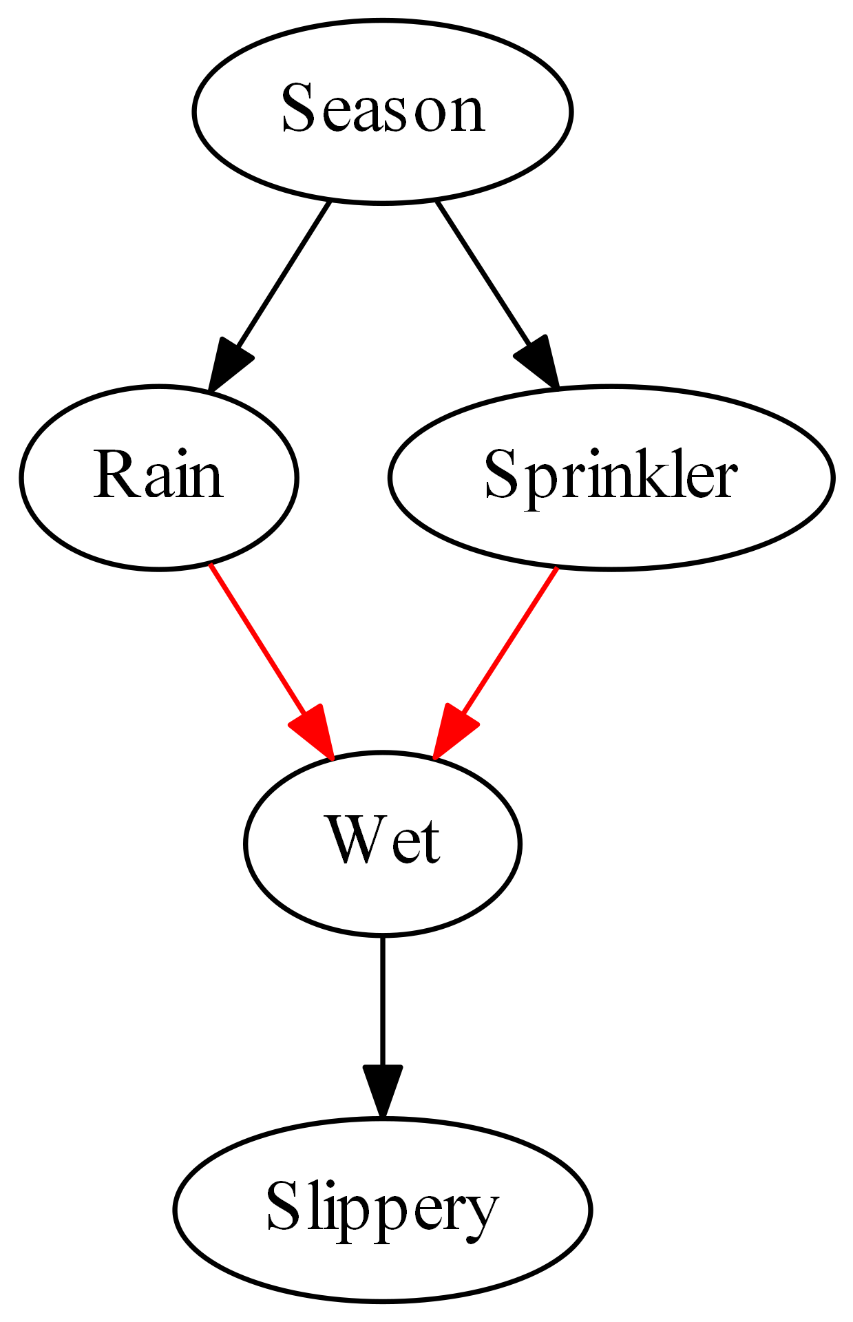
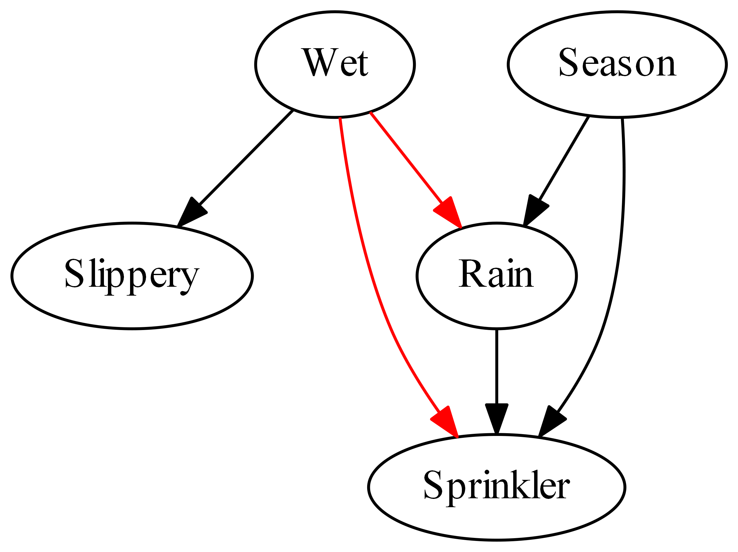
Figure 1: The recovered graphs correctly (left) or incorrectly (right) represent the data generating process. Edges prescribed by the respective sets of domain knowledge are marked in red, the rest of them has been added by the causal discovery algorithm.

In the next step, we estimate the target effect and our quantitative probes from the causal graph and the data via linear regression. We recover a target effect of $0.52$, but in principle, we have no idea whether this is a reasonable estimate or not. However, the analysis shows that the ATE of ’Sprinkler’ on ’Wet’ is $0.62$ and the ATE of ’Wet’ on ’Slippery’ is $0.81$. Therefore, our expectations about the known causal effects have been met by the predictions of the model, which increases our trust in the model and therefore also in the estimate of the target effect.

As a contrast, let us see how our probes help us detect flawed causal models: For this purpose, we intentionally communicate wrong assumptions about the causal graph to the causal discovery algorithm. For each edge that we have required in the above example, we now require the corresponding reversed edge. The same applies to the forbidden edges, which are also reversed. These flawed inputs lead to a flawed causal discovery result, as can be seen in Figure 1 (right).

If we now use the incorrect graph and the data to estimate the three ATE’s via linear regression, we observe a target effect of $0$ because there is no directed path from ’Sprinkler’ to ’Slippery’. The ATE of ’Wet’ on ’Slippery’ is again $0.81$ in accordance with our expectations. However, the ATE of ’Sprinkler’ on ’Wet’ is $0$, even though we expect it to be a positive number. We can use this failed validation as evidence that something in our end-to-end analysis must have gone wrong, and therefore the estimate of the target effect should not be trusted either. In practice, this could lead us to reexamine the qualitative domain knowledge that we have passed, which would then result in a causal discovery result that is closer to the true causal graph. Another possibility would be the examination of the estimation strategy that was used to compute the numerical estimate from the statistical estimand and the data. In our case, this would not lead to a correct estimate of the target effect because the error in the model lies in the graph, not in the estimation procedure. A third possibility would be a reexamination of our quantitative expectations, e.g. if we notice that our expectations were actually about the natural direct effect instead of the ATE. In any case, formulating our explicit quantitative knowledge about certain causal effects in the model, followed by an automated validation at the end of the end-to-end analysis, serves as a valuable evaluation step that can help us detect modelling errors.

5.2 Assumptions

In the previous example, we have made several implicit assumptions that are necessary to leverage the power of quantitative probing for causal model validation.

• We need to have quantitative knowledge about some causal effects between the observed variables, otherwise we cannot validate the corresponding expectations after the analysis. However, note that these expectations can be stated with any desired precision: We can demand an effect to be simply non-zero, to be positive, to be above a certain threshold or even to be situated within a narrow neighborhood of an exact target value.

• Estimating the probes should not be excessively complicated to perform in addition to the estimation of the target effect. In our example, we could reuse the causal graph that we had already constructed for target effect estimation, in order to identify unbiased statistical estimands for the probes. The estimation itself only required fitting linear regression models and reading off the respective coefficients for each probe. In a setting where the estimation of the probes is more costly, the benefit of using quantitative probing could be overshadowed by the required additional effort.

• The parts of the data generating process that are responsible for the target effect must be in some way related to the parts that are responsible for the probes. An example would be that all variables in the target effect and in the probes belong to the same connected component of the causal graph. Otherwise, our model might be perfectly accurate for the component that holds all the probes, but flawed in the separate component that produces the target effect.

6 Simulation study

In this chapter, we provide experimental backing for the concept of quantitative probing as a method of validating causal models.

6.1 Simulation setup

In order to have access to both a ground truth and easy parameterization of the experiments, we chose a setup consisting of the repeated execution and evaluation of the following parameterized simulation run:

• Choose $n$ (number of nodes), $p_{edge}$, (edge probability), $m$ (number of samples), $p_{hint}$ (hint probability), $p_{probe}$ (probe probability) and $\epsilon_{probe}$ (probe tolerance).

• Draw a random directed acyclic graph (DAG) with $n$ nodes $x_{1},...,x_{n}$. Random means that for each of the $n^{2}$ possible directed edges, we include the edge with a probability $p_{edge}$. After all the edges have been selected, check whether the result is a DAG. If not, repeat the procedure.

• Draw a random binary CPD for each node $x_{i}$. The entries $p(x_{i}=1|\Pi_{i}=\pi_{i})$, which fully determine the CPD, are sampled from a uniform distribution on $[0,1]$.

• Draw $m$ samples from the resulting joint distribution over $(x_{1},...,x_{n})$.

• Select a proportion $p_{hint}$ of all the edges (rounded down) in the causal graph and add their presence to the qualitative domain knowledge.

• Randomly choose a nontrivial target effect and $p_{probe}\cdot n^{2}$ (rounded down) other treatment-outcome pairs that will serve as quantitative probes. By nontrivial, we mean that there exists a directed path from the treatment to the outcome in the causal graph, because otherwise any causal effect is trivially zero.

• Calculate the corresponding ATEs for the target effect and the probes from the fully specified causal Bayesian network, in order to obtain a ground truth.

• Run a causal end-to-end analysis, using the $m$ observational samples and the qualitative domain knowledge, and report the discovered causal graph, the estimate of the target effect and the hit rate for the quantitative probes. The hit rate is defined as the proportion of probes that have been correctly recovered by the analysis. In order to account for numerical errors and statistical fluctuations, we allow an absolute deviation of $\epsilon_{probe}$ from the true value for a probe estimate to be considered successful.

• Report the number of edges that differ between the true and the discovered graph, as well as the absolute and relative error of the target effect estimate.

In this article, we report the results for experiments with $n=7$ nodes, an edge probability of $p_{edge}=0.1$, $m=1000$ samples per DAG, $p_{hint}=0.3$, meaning that we suppose that we know $30$% (rounded down) of the correct causal edges, $p_{probe}=0.5$, meaning that we use half of the possible causal effects as quantitative probes, and $\epsilon_{probe}=0.1$, meaning that we consider probe estimates successful if they deviate no more than $0.1$ from the true value on an additive scale. As in the previous example, the causal discovery was performed using fast greedy equivalence search [24] and all ATEs were estimated using linear regression. Our hypothesis is that an end-to-end analysis that results in a high hit rate for the quantitative probes is more likely to have found both the true causal graph and the true target effect.

6.2 Used software

The programmatic implementation of the simulation relies on several open-source Python packages: At the beginning of the pipeline, the networkx package [26] was used for sampling DAGs based on the edge probability $p_{edge}$. The pgmpy package [23] enabled us to build a probabilistic graphical model from the given DAG by adding random CPDs for each node. The resulting model was then used to sample data for creating the observational dataset, as well as for obtaining the true ATEs by simulating data from interventional distributions. The causal end-to-end analysis and the validation of the quantitative probes were executed with the help of cause2e [10]. All plots were generated using Matplotlib [27]. In order to make the setup reusable, easily parametrizable and open for extension by other researchers, an open-source Python package for quantitative probing was developed around the above software setup (see Chapter 9).

6.3 Results

In order to support the above hypothesis, we plot the aggregated results of 1378 runs. Figure 2 shows the information for every single run as a separate data point: The $x$-coordinate indicates the hit rate of the run in each of the four plots, whereas the $y$-coordinate describes varying quantities of interest:

• The plot to the upper left shows the absolute difference between the estimated and the true value of the target effect.

• The plot to the upper right shows the relative difference $\lvert\frac{\hat{\tau}-\tau}{\tau}\rvert$ between the estimated value $\hat{\tau}$ and the true value $\tau$ of the target effect. Note that no division by zero happens, since all target effects were chosen to be nontrivial.

• The plot to the lower left shows the structural hamming distance [28] between the true and the discovered graph. This includes both, edges that are present in only one of the graphs, as well as reversed edges.

• The plot to the lower right is the only aggregation: It shows the absolute frequencies of the hit rates over all runs.

As we can see, the data in the upper plots does not seem to support our hypothesis at all: We expect to see the points following a trend from the upper left (few successful probes, large estimation error) to the lower right (many successful probes, small estimation error), but there seems to be no downward trend. On the contrary, Figure 2 (upper left) even shows a higher number of significant estimation errors when the hit rate is high. At least the second concern can be resolved by a look at the hit rate frequencies in Figure 2 (lower right): Almost all of the runs show a hit rate of at least $0.8$. The high ratio of successful probes is likely connected to the fact that many of the randomly chosen treatment-outcome-pairs in the probes are not connected by a directed path in the true graph. Even if the discovered graph is not completely correct, it is sufficient not to introduce a directed path by mistake, in order to estimate the probe successfully. Therefore, the higher number of significant relative estimation errors in the plot can be explained by the higher number of data points for the corresponding hit rates. Similarly, the above-mentioned apparent lack of a downward trend is simply due to visualization problems caused by the high number of data points. In order to resolve this issue, we replace the many single data points for each hit rate by one data point whose $y$-coordinate is the mean value over the plotted quantity for the given hit rate. The results are shown in Figure 3: Since the plots are derived from the same runs as before, the hit rate histogram in Figure 3 (bottom right) is unchanged. The other three plots now show the expected downward trend for the regions that contain a sufficient number of samples, indicating that runs with a higher hit rate performed better at estimating the target effect and recovering the causal graph from data and domain knowledge. It even seems that the relationship between the hit rate and the other variables is approximately linear, but a theoretical foundation for this observation could not be established.

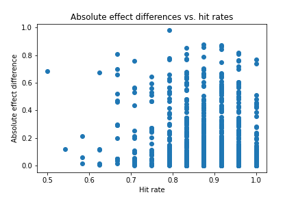
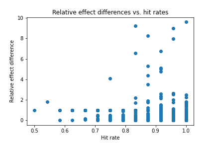
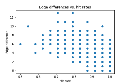
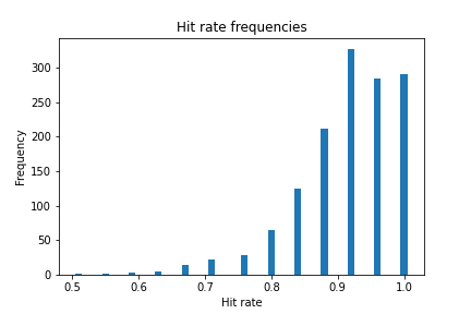
Figure 2: The top row shows plots of the absolute (left) and relative (right) differences between the true target effect and the estimated result against the hit rate. The bottom row shows a plot of the structural hamming distance between the true causal graph and the causal discovery result against the hit rate (left), as well as a histogram of the observed hit rates (right).

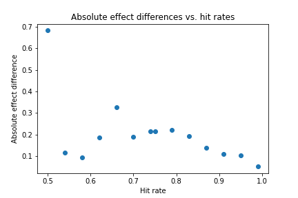
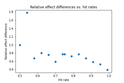
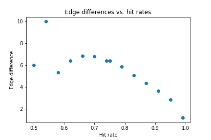
Figure 3: Aggregated results: The top row shows plots of the mean absolute (left) and relative (right) difference between the true target effect and the estimated result against the hit rate. The bottom row shows a plot of the mean structural hamming distances between the true causal graph and the causal discovery result against the hit rate (left), as well as a histogram of the observed hit rates (right).

6.4 Outlier analysis

The results indicate that the probability of having recovered both, the true causal graph and the correct target effect, from observational data and domain knowledge increases with the amount of correctly estimated quantitative probes, i.e. the hit rate. However, the presented evidence only supports this in a probabilistic manner and even a perfect estimation of all probes does not guarantee a successful causal analysis. This contrast is reflected in the above plots: On the one hand, the mean errors in Figure 3 approach $0$, as the hit rate approaches $1$. On the other hand, the non-aggregated plots in Figure 2 show numerous data points with a hit rate of $1$ and considerable errors in both, graph and target effect recovery. More precisely, our data contains $14$ runs that simultaneously have a perfect hit rate of $1$ and an absolute estimation error of at least $0.2$. In order to understand the thereby evidenced limitations of the quantitative probing approach, we look at some of these outliers more closely.

6.4.1 Connectivity

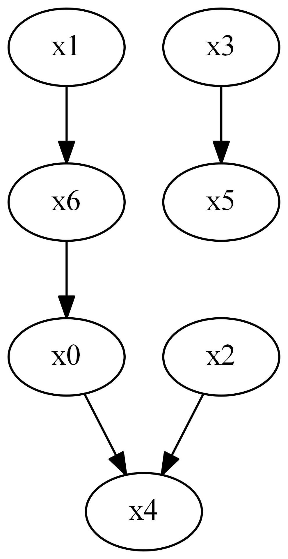
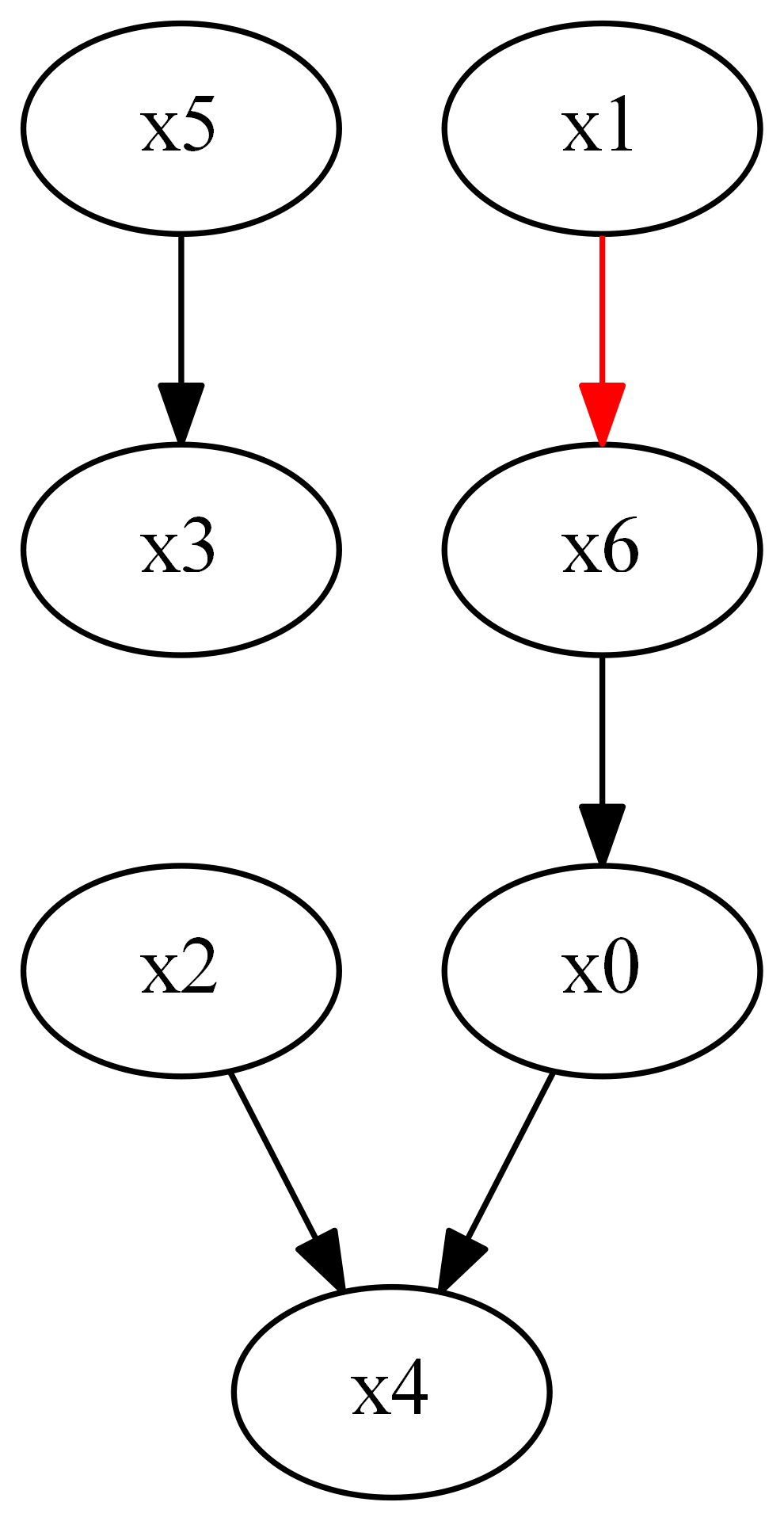
Figure 4: Plot of the true (left) and discovered (right) causal graphs for an outlier run with treatment $x_{3}$ and outcome $x_{5}$. In the discovered graph, the red edge $x_{1}\rightarrow x_{6}$ has been required by domain knowledge. The edge $x_{3}\rightarrow x_{5}$ has been oriented incorrectly.

Consider the run depicted in Figure 4: The target effect was the ATE of $x_{3}$ on $x_{5}$, which has been incorrectly estimated to be $0$ instead of $0.5$, although all of the probes have been correctly estimated. An examination of the graph structures immediately explains the phenomenon. The true graph and the discovered graph are identical, except for one edge between $x_{3}$ and $x_{5}$, which has been reversed by the causal discovery algorithm. This is not surprising, as the two structures are Markov equivalent and could only have been discerned by passing the correct orientation of the edge as domain knowledge. However, the only edge included in the domain knowledge is the edge between $x_{1}$ and $x_{6}$ (red). As a result, all of the probes have been estimated correctly, leading to a perfect hit rate of $1$. Of course, the perfect performance in one connected component of the causal graph has no benefits for a task that relates only to the other component of the graph, such as the estimation of our target causal effect. These findings illustrate that it is not only important to correctly recover the probes, but also to select helpful probes in the first place. Given that we have not enforced any connectivity constraints during DAG generation, it is plausible that the proposed validation technique has encountered problems in graphs with multiple connected components.

In order to confirm these explanations, we filter out all experiment runs where the true causal graph consists of more than one connected component, and recreate Figures 2 and 3 from the reduced dataset of 653 runs. The resulting Figures 5 and 6 indeed show fewer deviations from the bottom right, indicating that a sizeable proportion of the runs where our validation approach failed were linked to the problem of disconnected graphs. If we apply the above outlier filter, we are left with only $4$ runs with perfect hit rate and an absolute estimation error of over $0.2$. In practice, this suggests that we should choose probes that we suspect to be in the same component of the causal graph as the target variables. It seems plausible that even within one component, the probes that are closer to the target effect will be more useful for judging the correctness of the model.

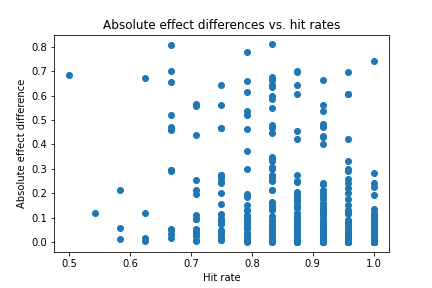
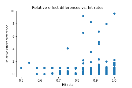
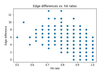
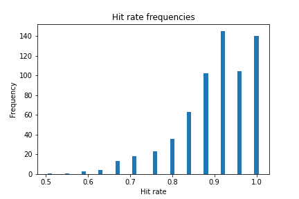
Figure 5: Results for all runs with connected causal graphs: The top row shows plots of the absolute (left) and relative (right) differences between the true target effect and the estimated result against the hit rate. The bottom row shows a plot of the number of structural hamming distances between the true causal graph and the causal discovery result against the hit rate (left), as well as a histogram of the observed hit rates (right).

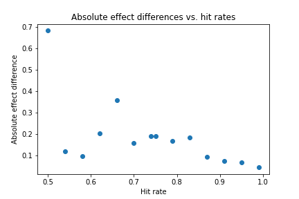
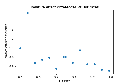
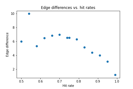
Figure 6: Aggregated results for all runs with connected causal graphs: The top row shows plots of the mean absolute (left) and relative (right) difference between the true target effect and the estimated result against the hit rate. The bottom row shows a plot of the mean structural hamming distances between the true causal graph and the causal discovery result against the hit rate (left), as well as a histogram of the observed hit rates (right).

6.4.2 Probe coverage

In order to understand the remaining outliers, we offer two explanations: The first one is related to the probe coverage. Given that in most applications, it is unrealistic to assume that the analyst knows all causal effects except for the target effect, we have selected only $24$ of the $7\cdot 7=49$ causal effects as probes. This suggests that some of the erroneous analyses in the outlier runs could have been captured by increasing the number of probes, as is illustrated in Figure 7: The estimation of the ATE of $x_{5}$ on $x_{6}$ has yielded a result of $0$ instead of the true value $0.28$, although all the probes have been correctly estimated. A closer look at the 24 probes reveals that the ATE of $x_{3}$ on $x_{6}$ has not been used as a probe. This probe could have detected the incorrect graph, since its effect is trivially zero in the discovered graph, but non-zero in the true graph.

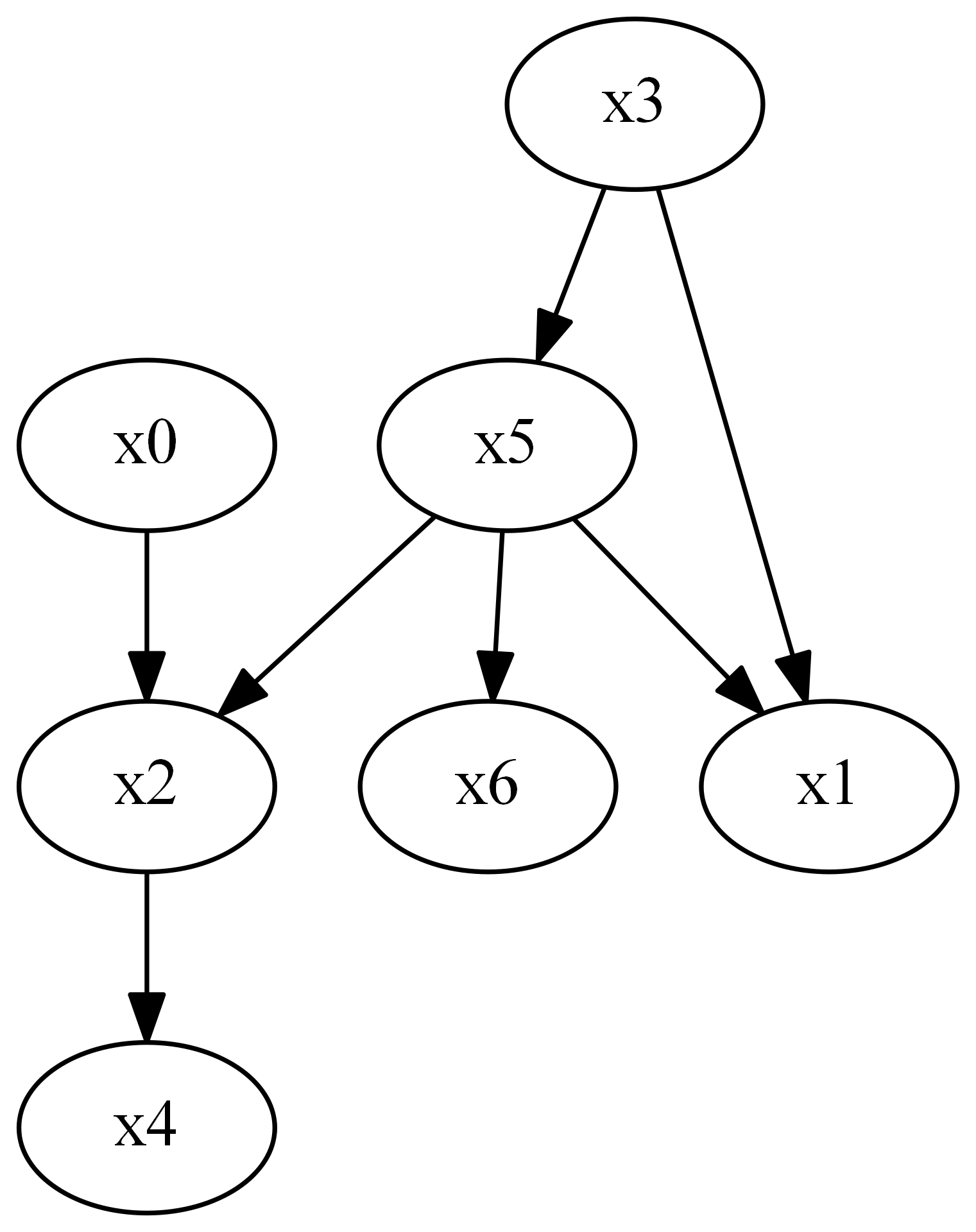
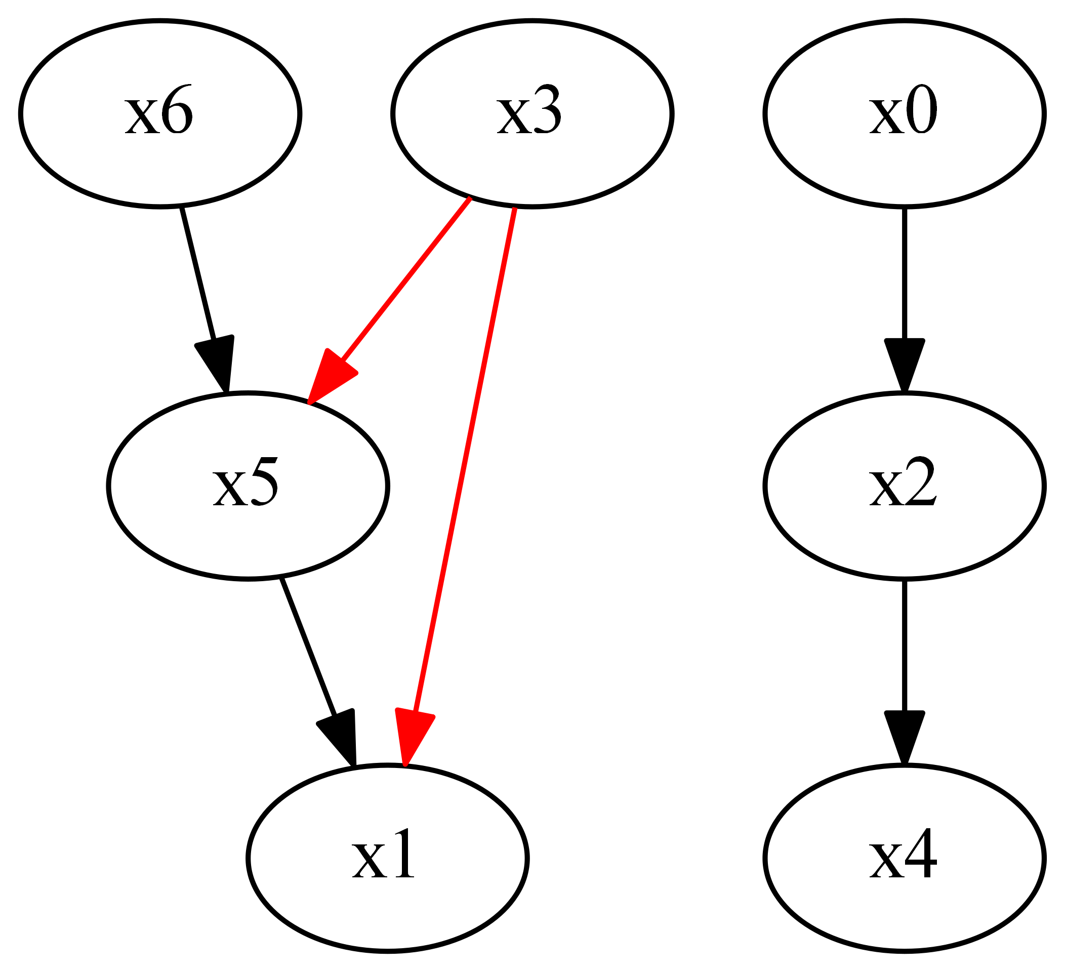
Figure 7: Plot of the true (left) and discovered (right) causal graphs for an outlier run with treatment $x_{5}$ and outcome $x_{6}$. In the discovered graph, the red edges $x_{3}\rightarrow x_{5}$ and $x_{3}\rightarrow x_{1}$ have been required by domain knowledge. The edge $x_{5}\rightarrow x_{6}$ has been oriented incorrectly and the edge $x_{5}\rightarrow x_{2}$ is missing.

6.4.3 Probe tolerance

The second explanation focusses on the definition of the hit rate, which is clearly a deciding factor for marking a run as an outlier. The hit rate is high if many probes have been correctly estimated, and "correctly" means that the estimate has to lie within some reasonable bounds around the true effect. While this seems straightforward, the problem lies in the definition of the bounds: Should we specify an absolute error margin that applies to all of the probes? Or should we specify a relative margin that depends on the size of each of the probe effects? Using an absolute margin of $\epsilon_{probe}=0.1$ to both sides, as we did in our experiments, can be a good fit for a true effect size of $1$, but it might be dangerous for a true effect size of $0.001$ (underreject) or $1000$ (overreject).

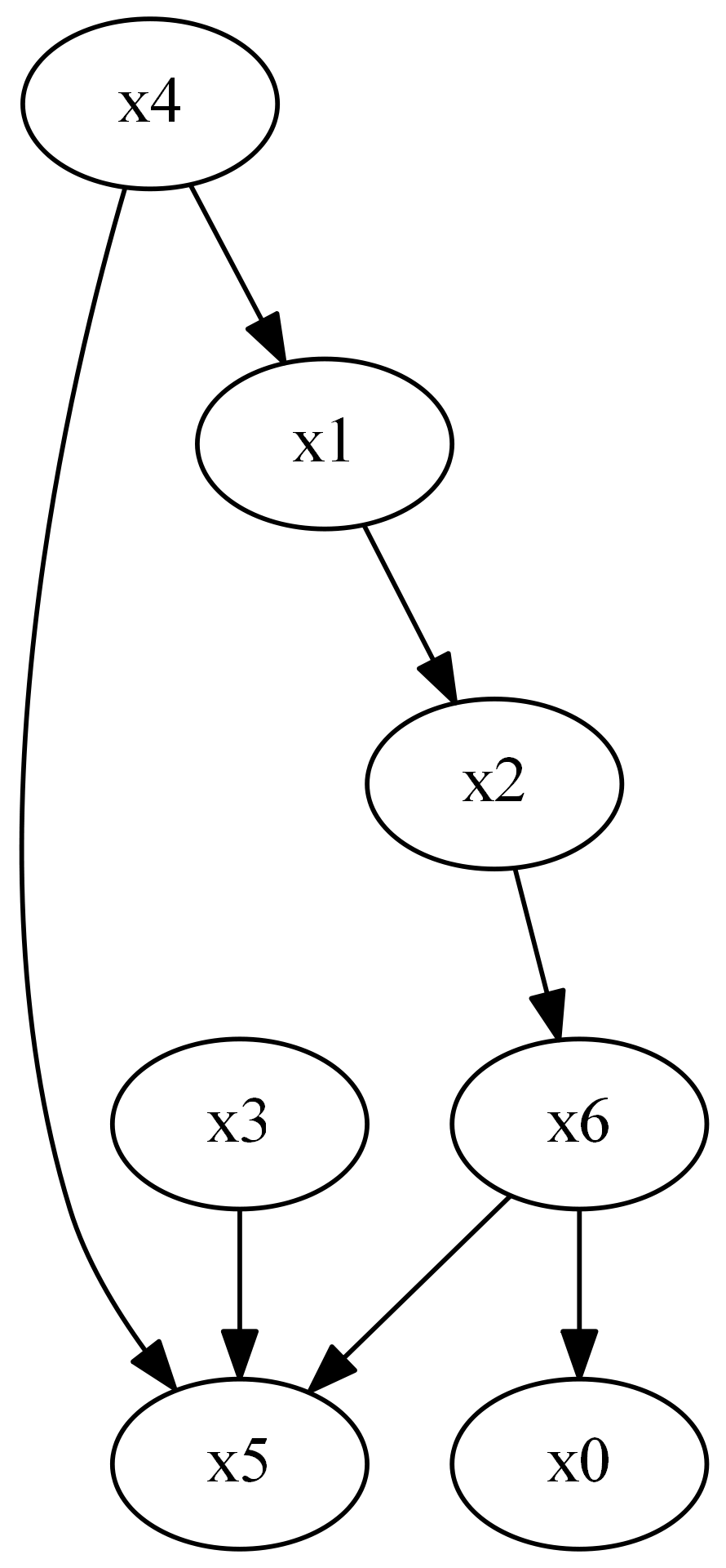
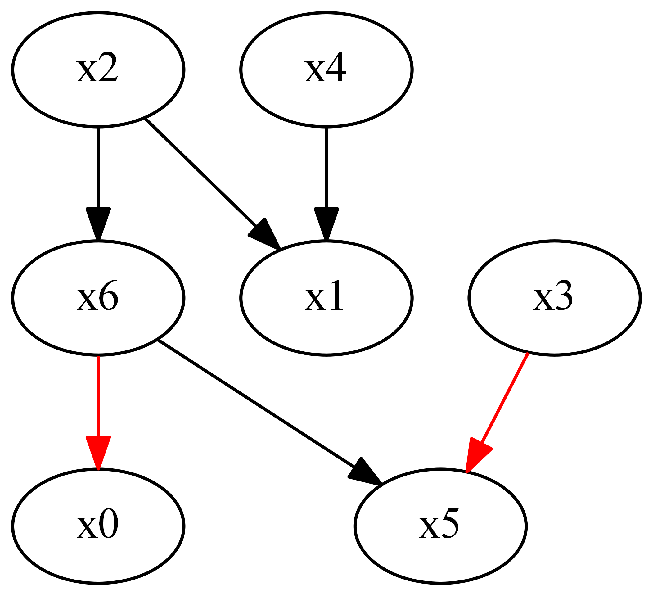
Figure 8: Plot of the true (left) and discovered (right) causal graphs for an outlier run with treatment $x_{1}$ and outcome $x_{2}$. In the discovered graph, the red edges $x_{6}\rightarrow x_{0}$ and $x_{3}\rightarrow x_{5}$ have been required by domain knowledge. The edge $x_{1}\rightarrow x_{2}$ has been oriented incorrectly and the edge $x_{4}\rightarrow x_{5}$ is missing.

To illustrate this line of thought, we look at the run in Figure 8: The ATE of $x_{1}$ on $x_{2}$ was erroneously estimated to be $0$ instead of $-0.24$, although all of the probes were estimated correctly. In this case, it is remarkable that the ATE of $x_{4}$ and $x_{2}$ was one of the probes. This probe is trivially $0$ in the discovered graph, as there is no directed path from $x_{4}$ to $x_{2}$. In the true graph, however, it can only vanish in the degenerate case. Indeed, the true effect is $0.07$. Given our generic bounds determined by $\epsilon_{probe}=0.1$, the incorrect estimate of $0$ falls within the acceptance interval $[-0.03,0.17]$ and the error goes unnoticed. This could have been avoided by specifying proper bounds for each of the probes, a task whose feasibility in practice depends on the available domain knowledge. It is worth noting that all the inspected outliers either show a true or an estimated target effect that is trivially $0$. The absence of more subtle estimation problems where the directed path exists in both, the true and the recovered graph, but the estimation is jeopardized by a difference in backdoor paths, is probably due to the low number of variables in the generated DAGs. However, quantitative probing is applicable without any modifications to more complicated graph structures.

7 Conclusion and outlook

In summary, we have introduced the method of quantitative probing for validating causal models. We identified the additional difficulties in validating causal models when compared to traditional correlation-based machine learning models by reviewing the role of the i.i.d. assumption. In analogy to the model-agnostic train/test split, we proposed a validation strategy that allows us to treat the underlying causal model as a black box that answers causal queries. The strategy was put into context as an extension of the already existing technique of using refutation checks, which is in line with the established logic of scientific discovery. After illustrating the motivation behind the concept of quantitative probing using Pearl’s sprinkler example, we presented and discussed the results of a thorough simulation study. While being mostly supportive of our hypothesis that quantitative probes can be used as an indicator for model fitness, the study also revealed shortcomings of the method, which were further analyzed using exemplary failing runs.

To conclude the article, we revisit the assumptions from Chapter 5.2 and the ideas from Chapter 6.4, in order to identify topics for future research.

• Is there a way to explain the roughly linear association between the hit rate and the edge/effect differences in Figure 3? Answering this question would provide a solid theoretical backing for the quantitative probing method, in addition to the simulation-based evidence presented in this article.

• Can we quantify the "usefulness" of each employed quantitative probe for detecting wrong models? An example would be to plot the results for a single fixed hit rate, but each data point could represent runs that used only specific probes, e.g. only those whose variables lie within a maximum distance from the target variables. What other criteria could make a specific probe useful? Answering this question would aid practitioners in eliciting specific quantitative knowledge from domain experts.

• Given the probe coverage issue in Figure 7, is there a way to model how the effectiveness of the method depends on the number of used quantitative probes? Answering this question would aid practitioners in gauging the amount of required quantitative domain knowledge for model validation.

• Given the probe tolerance issues in Figure 8, how much more useful do the probes become for detecting wrong models if we narrow the allowed bounds in the validation effects? How can we determine ideal bounds to avoid overreject and underreject? Answering this question would provide important guidance to both researchers and practitioners, as the bounds must be actively chosen by the investigator in each application of quantitative probing.

Similarly to how qualitative knowledge by domain experts can assist causal discovery procedures in recovering the correct causal graph from observational data, we believe that quantitative probing can serve as a natural method of incorporating quantitative domain knowledge into causal analyses. By answering the above questions, the proposed validation strategy can evolve into a tool that builds trust in causal models, thereby facilitating the adoption of causal inference techniques in various application domains.

8 Acknowledgments

We are grateful for the support of our colleagues at ams OSRAM and the University of Regensburg. Sebastian Imhof helped sharpen the idea of using known causal effects for model validation during multiple fruitful conversations. Other validation approaches for causal models were compared in several meetings of our causal inference working group [29]. The idea of different degrees of usefulness for different types of quantitative probes was brought up in a discussion with members of the Department of Statistical Bioinformatics at the University of Regensburg. Heribert Wankerl deserves special credit for proofreading the paper.

9 Code and data availability

All of the above results can be reproduced by running two notebooks in the companion GitHub repository of this article, which also contains the open-source qprobing Python package [11]. The qprobing package relies on the open-source cause2e Python package for performing the causal end-to-end analysis, which is hosted in a separate GitHub repository [10].

References

- [1] Judea Pearl. Causality. Cambridge University Press, Cambridge, UK, 2nd edition, 2009.
- [2] Joshua D. Angrist, Guido W. Imbens, and Donald B. Rubin. Identification of causal effects using instrumental variables. Journal of the American Statistical Association, 91(434):444–455, 1996.
- [3] Donald B Rubin. Causal inference using potential outcomes. Journal of the American Statistical Association, 100(469):322–331, 2005.
- [4] P. Spirtes, C. Glymour, and R. Scheines. Causation, Prediction, and Search. MIT press, 2nd edition, 2000.
- [5] J. Peters, D. Janzing, and B. Schölkopf. Elements of Causal Inference - Foundations and Learning Algorithms. Adaptive Computation and Machine Learning Series. The MIT Press, Cambridge, MA, USA, 2017.
- [6] Paul W. Holland. Statistics and causal inference. Journal of the American Statistical Association, 81(396):945–960, 1986.
- [7] J. M. Kendall. Designing a research project: randomised controlled trials and their principles. Emergency Medicine Journal, 20(2):164–168, 2003.
- [8] Trevor Hastie, Robert Tibshirani, and Jerome H. Friedman. The Elements of Statistical Learning: Data Mining, Inference, and Prediction, 2nd Edition. Springer Series in Statistics. Springer, 2009.
- [9] K. R. Popper. The Logic of Scientific Discovery. Hutchinson, London, 1934.
- [10] Daniel Grünbaum. cause2e: A python package for causal end-to-end analysis, 2021. Available at https://github.com/MLResearchAtOSRAM/cause2e.
- [11] Daniel Grünbaum. qprobing: A python package for evaluating the effectiveness of quantitative probing for causal model validation, 2022. Available at https://github.com/MLResearchAtOSRAM/qprobing.
- [12] Andrew Jesson, Sören Mindermann, Yarin Gal, and Uri Shalit. Quantifying ignorance in individual-level causal-effect estimates under hidden confounding. arXiv:2103.04850, 2021.
- [13] Carlos Cinelli and Chad Hazlett. Making sense of sensitivity: extending omitted variable bias. Journal of the Royal Statistical Society Series B, 82(1):39–67, 2020.
- [14] Victor Chernozhukov, Carlos Cinelli, Whitney Newey, Amit Sharma, and Vasilis Syrgkanis. Long story short: Omitted variable bias in causal machine learning. arXiv:2112.13398, 2021.
- [15] Victor Veitch and Anisha Zaveri. Sense and sensitivity analysis: Simple post-hoc analysis of bias due to unobserved confounding. In H. Larochelle, M. Ranzato, R. Hadsell, M.F. Balcan, and H. Lin, editors, Advances in Neural Information Processing Systems, volume 33, pages 10999–11009. Curran Associates, Inc., 2020.
- [16] Brady Neal, Chin-Wei Huang, and Sunand Raghupathi. Realcause: Realistic causal inference benchmarking. arXiv:2011.15007, 2020.
- [17] Amit Sharma, Vasilis Syrgkanis, Cheng Zhang, and Emre Kıcıman. Dowhy: Addressing challenges in expressing and validating causal assumptions. arXiv:2108.13518, 2021.
- [18] Jason Abrevaya, Yu-Chin Hsu, and Robert P. Lieli. Estimating conditional average treatment effects. Journal of Business & Economic Statistics, 33(4):485–505, 2015.
- [19] David Heckerman. A bayesian approach to learning causal networks. In Proceedings of the Eleventh Conference on Uncertainty in Artificial Intelligence, UAI’95, page 285–295, San Francisco, CA, USA, 1995. Morgan Kaufmann Publishers Inc.
- [20] Clark Glymour, Kun Zhang, and Peter Spirtes. Review of causal discovery methods based on graphical models. Frontiers in Genetics, 10, 2019.
- [21] Matthew J. Vowels, Necati Cihan Camgoz, and Richard Bowden. D’ya like dags? a survey on structure learning and causal discovery, 2021.
- [22] Christopher Meek. Causal inference and causal explanation with background knowledge. In Proceedings of the Eleventh Conference on Uncertainty in Artificial Intelligence, UAI’95, page 403–410, San Francisco, CA, USA, 1995. Morgan Kaufmann Publishers Inc.
- [23] Ankur Ankan and Abinash Panda. pgmpy: Probabilistic graphical models using python. In Proceedings of the 14th Python in Science Conference (SCIPY 2015), 2015.
- [24] Joseph Ramsey, Madelyn Glymour, Ruben Sanchez-Romero, and Clark Glymour. A million variables and more: the fast greedy equivalence search algorithm for learning high-dimensional graphical causal models, with an application to functional magnetic resonance images. International Journal of Data Science and Analytics, 3, 03 2017.
- [25] David Maxwell Chickering. Optimal structure identification with greedy search. J. Mach. Learn. Res., 3:507–554, March 2003.
- [26] Aric A. Hagberg, Daniel A. Schult, and Pieter J. Swart. Exploring network structure, dynamics, and function using networkx. In Gaël Varoquaux, Travis Vaught, and Jarrod Millman, editors, Proceedings of the 7th Python in Science Conference, pages 11 – 15, Pasadena, CA USA, 2008.
- [27] J. D. Hunter. Matplotlib: A 2d graphics environment. Computing in Science & Engineering, 9(3):90–95, 2007.
- [28] Ioannis Tsamardinos, Laura E. Brown, and Constantin F. Aliferis. The max-min hill-climbing bayesian network structure learning algorithm. Mach. Learn., 65(1):31–78, oct 2006.
- [29] Daniel Grünbaum. Causal inference working group. Available at https://gitlab.com/causal-inference/working-group/-/wikis/home.