Flow Straight and Fast:
Learning to Generate and Transfer Data with Flow

Abstract

We present rectified flow, a surprisingly simple approach to learning (neural) ordinary differential equation (ODE) models to transport between two empirically observed distributions ${\pi}_{0}$ and ${\pi}_{1}$, hence providing a unified solution to generative modeling and domain transfer, among various other tasks involving distribution transport. The idea of rectified flow is to learn the ODE to follow the straight paths connecting the points drawn from ${\pi}_{0}$ and ${\pi}_{1}$ as much as possible. This is achieved by solving a straightforward nonlinear least squares optimization problem, which can be easily scaled to large models without introducing extra parameters beyond standard supervised learning. The straight paths are special and preferred because they are the shortest paths between two points, and can be simulated exactly without time discretization and hence yield computationally efficient models. We show that the procedure of learning a rectified flow from data, called rectification, turns an arbitrary coupling of ${\pi}_{0}$ and ${\pi}_{1}$ to a new deterministic coupling with provably non-increasing convex transport costs. In addition, recursively applying rectification allows us to obtain a sequence of flows with increasingly straight paths, which can be simulated accurately with coarse time discretization in the inference phase. In empirical studies, we show that rectified flow performs superbly on image generation, image-to-image translation, and domain adaptation. In particular, on image generation and translation, our method yields nearly straight flows that give high quality results even with a single Euler discretization step.

1 Introduction

Compared with supervised learning, the shared difficulty of various forms of unsupervised learning is the lack of paired input/output data with which standard regression or classification tasks can be invoked. The gist of most unsupervised methods is to find, in one way or another, meaningful correspondences between points from two distributions. For example, generative models such as generative adversarial networks (GAN) and variational autoencoders (VAE) [e.g., 19, 32, 14] seek to map data points to latent codes following a simple elementary (Gaussian) distribution with which the data can be generated and manipulated. Representation learning rests on the idea that if a sufficiently smooth function can map a structured data distribution to an elementary distribution, it can (likely) be endowed with certain semantically meaningful interpretation and useful for various downstream learning tasks. On the other hand, domain transfer methods find mappings to transfer points from two different data distributions, both observed empirically, for the purpose of image-to-image translation, style transfer, and domain adaption [e.g., 100, 16, 79, 59]. All these tasks can be framed unifiedly as finding a transport map between two distributions:

The Transport Mapping Problem Given empirical observations of two distributions $X_{0}\sim{\pi}_{0},X_{1}\sim{\pi}_{1}$ on $\mathbb{R}^{d}$, find a transport map $T\colon\mathbb{R}^{d}\to\mathbb{R}^{d}$ (hopefully nice or optimal in certain sense), such that $Z_{1}\coloneqq T(Z_{0})\sim{\pi}_{1}$ when $Z_{0}\sim{\pi}_{0}$, that is, $(Z_{0},Z_{1})$ is a coupling (a.k.a transport plan) of ${\pi}_{0}$ and ${\pi}_{1}$.

Several lines of techniques have been developed depending on how to represent and train the map $T$. In traditional generative models, $T$ is parameterized as a neural network, and trained with either GAN-type minimax algorithms or (approximate) maximum likelihood estimation (MLE). However, GANs are known to suffer from numerically instability and mode collapse issues, and require substantial engineering efforts and human tuning, which often do not transfer well across different model architecture and datasets. On the other hand, MLE tends to be intractable for complex models, and hence requires approximate variational or Monte Carlo inference techniques such as those used in variational auto-encoders (VAE), or special model structures such as normalizing flow and auto-regressive models, to yield tractable likelihood, causing difficult trade-offs between expressive power and computational cost.

Recently, advances have been made by representing the transport plan implicitly as a continuous time process, such as flow models with neural ordinary differential equations (ODEs) [e.g., 6, 56] and diffusion models by stochastic differential equations (SDEs) [e.g., 73, 23, 80, 11, 82]; in these models, a neural network is trained to represent the drift force of the processes and a numerical ODE/SDE solver is used to simulate the process during inference. The key idea is that, by leveraging the mathematical structures of ODEs/SDEs, the continuous-time models can be trained efficiently without resorting to minimax or traditional approximate inference techniques. The most notable examples are the recent score-based generative models [71, 72, 73] and denoising diffusion probabilistic models (DDPM) [23], which we call denoising diffusion methods collectively. These methods allow us to train large-scale diffusion/SDE-based generative models that surpass GANs on image generation in both image quality and diversity, without the instability and mode collapse issues [e.g., 12, 53, 61, 64]. The learned SDEs can be converted into deterministic ODE models for faster inference with the method of probability flow ODEs [73] and DDIM [70].

However, compared with the traditional one-step models like GAN and VAE, a key drawback of continuous-times models is the high computational cost in inference time: drawing a single point (e.g., image) requires to solve the ODE/SDE with a numerical solver that needs to repeatedly call the expensive neural drift function. In addition, the existing denoising diffusion techniques require substantial hyper-parameter search in an involved design space and are still poorly understood both empirically and theoretically [29].

In existing approaches, generative modeling and domain transfer are typically treated separately. It often requires to extend or customize a generative learning techniques to solve domain transfer problems; see e.g., Cycle GAN [100] and diffusion-based image-to-image translation [e.g., 75, 97]. One framework that naturally unifies both domains is optimal transport (OT) [e.g., 85, 2, 15, 59], which endows a collection of techniques for finding optimal couplings with minimum transport costs of form $\mathbb{E}[c(Z_{1}-Z_{0})]$ w.r.t. a cost function $c\colon\mathbb{R}^{d}\to\mathbb{R}$, yielding natural applications to both generative and transfer learning. However, the existing OT techniques are slow for problems with high dimensional and large volumes of data [59]. Furthermore, as the transport costs do not perfectly align with the actual learning performance, methods that faithfully find the optimal transport maps do not necessarily have better learning performance [34].

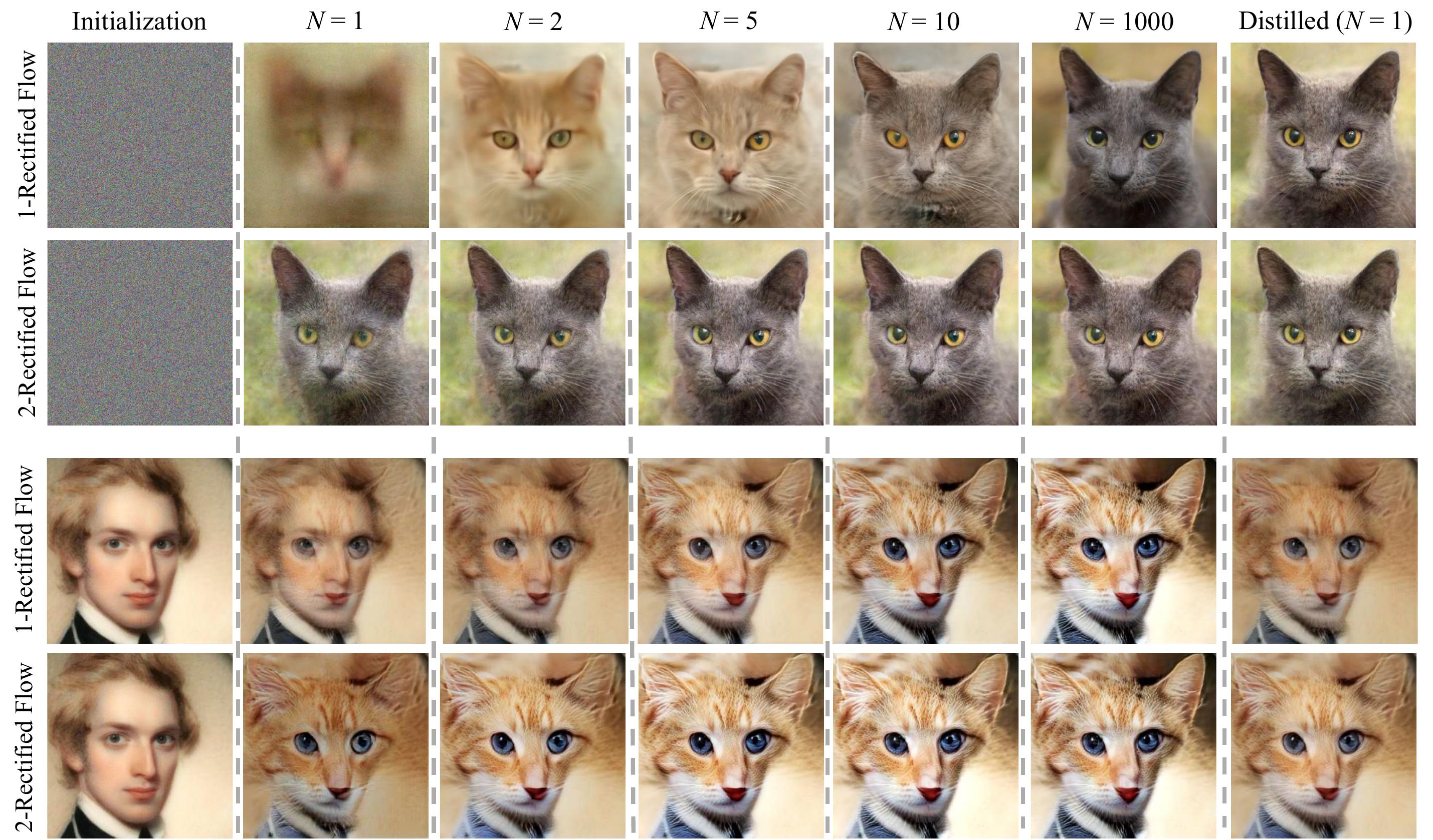
Figure 1: The trajectories of rectified flows for image generation (${\pi}_{0}$: standard Gaussian noise, ${\pi}_{1}$: cat faces, top two rows), and image transfer between human and cat faces (${\pi}_{0}$: human faces, ${\pi}_{1}$: cat faces, bottom two rows), when simulated using Euler method with step size $1/N$ for $N$ steps. The first rectified flow induced from the training data (1-rectified flow) yields good results with a very small number (e.g., $\geq 2$) of steps; the straightened reflow induced from 1-rectified flow (denoted as 2-rectified flow) has nearly straight line trajectories and yield good results even with one discretization step.

Contribution

We introduce rectified flow, a surprisingly simple approach to the transport mapping problem, which unifiedly solves both generative modeling and domain transfer. The rectified flow is an ODE model that transport distribution ${\pi}_{0}$ to ${\pi}_{1}$ by following straight line paths as much as possible. The straight paths are preferred both theoretically because it is the shortest path between two end points, and computationally because it can be exactly simulated without time discretization. Hence, flows with straight paths bridge the gap between one-step and continuous-time models.

Algorithmically, the rectified flow is trained with a simple and scalable unconstrained least squares optimization procedure, which avoids the instability issues of GANs, the intractable likelihood of MLE methods, and the subtle hyper-parameter decisions of denoising diffusion models. The procedure of obtaining the rectified flow from the training data has the attractive theoretical property of 1) yielding a coupling with non-increasing transport cost jointly for all convex cost $c$, and 2) making the paths of flow increasingly straight and hence incurring lower error with numerical solvers. Therefore, with a reflow procedure that iteratively trains new rectified flows with the data simulated from the previously obtained rectified flow, we obtain nearly straight flows that yield good results even with the coarsest time discretization, i.e., one Euler step. Our method is purely ODE-based, and is both conceptually simpler and practically faster in inference time than the SDE-based approaches of [23, 73, 70].

Empirically, rectified flow can yield high-quality results for image generation when simulated with a very few number of Euler steps (see Figure 1, top row). Moreover, with just one step of reflow, the flow becomes nearly straight and hence yield good results with a single Euler discretization step (Figure 1, the second row). This substantially improves over the standard denoising diffusion methods. Quantitatively, we claim a state-of-the-art result of FID (4.85) and recall (0.51) on CIFAR10 for one-step fast diffusion/flow models [5, 48, 91, 99, 47]. The same algorithm also achieves superb result on domain transfer tasks such as image-to-image translation (see the bottom two rows of Figure 1) and transfer learning.

2 Method

We provide a quick overview of the method in Section 2.1, followed with some discussion and remarks in Section 2.2. We introduce a nonlinear extension of our method in Section 2.3, with which we clarify the connection and advantages of our method with the method of probability flow ODEs [73] and DDIM [70].

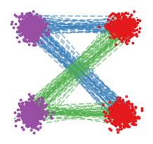
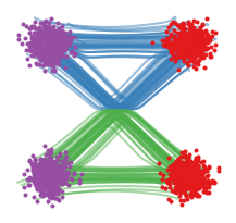
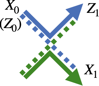
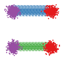
(a) Linear interpolation $X_{t}=tX_{1}+(1-t)X_{0}$	(b) Rectified flow $Z_{t}$ induced by $(X_{0},X_{1})$	(c) Linear interpolation $Z_{t}=tZ_{1}+(1-t)Z_{0}$	(d) Rectified flow $Z^{\prime}_{t}$ induced by $(Z_{0},Z_{1})$

Figure 2: (a) Linear interpolation of data input $(X_{0},X_{1})\sim{\pi}_{0}\times{\pi}_{1}$. (b) The rectified flow $Z_{t}$ induced by $(X_{0},X_{1})$; the trajectories are “rewired” at the intersection points to avoid the crossing. (c) The linear interpolation of the end points $(Z_{0},Z_{1})$ of flow $Z_{t}$. (d) The rectified flow induced from $(Z_{0},Z_{1})$, which follows straight paths.

2.1 Overview

Rectified flow

Given empirical observations of $X_{0}\sim{\pi}_{0},X_{1}\sim{\pi}_{1}$, the rectified flow induced from $(X_{0},X_{1})$ is an ordinary differentiable model (ODE) on time $t\in[0,1]$,

$$\mathrm{d}Z_{t}=v(Z_{t},t)\mathrm{d}t,$$

which converts $Z_{0}$ from ${\pi}_{0}$ to a $Z_{1}$ following ${\pi}_{1}$. The drift force $v\colon\mathbb{R}^{d}\to\mathbb{R}^{d}$ is set to drive the flow to follow the direction $(X_{1}-X_{0})$ of the linear path pointing from $X_{0}$ to $X_{1}$ as much as possible, by solving a simple least squares regression problem:

$$\min_{v}\int_{0}^{1}\mathbb{E}\left[\left\lVert(X_{1}-X_{0})-v\big{(}X_{t},\leavevmode\nobreak\ t\big{)}\right\rVert^{2}\right]\mathrm{d}t,\leavevmode\nobreak\ \leavevmode\nobreak\ \leavevmode\nobreak\ \leavevmode\nobreak\ \leavevmode\nobreak\ \text{with}\leavevmode\nobreak\ \leavevmode\nobreak\ \leavevmode\nobreak\ \leavevmode\nobreak\ X_{t}=tX_{1}+(1-t)X_{0},$$ (1)

where $X_{t}$ is the linear interpolation of $X_{0}$ and $X_{1}$. Naviely, $X_{t}$ follows the ODE of $\mathrm{d}X_{t}=(X_{1}-X_{0})\mathrm{d}t,$ which is non-causal (or anticipating) as the update of $X_{t}$ requires the information of the final point $X_{1}$. By fitting the drift $v$ with $X_{1}-X_{0}$, the rectified flow causalizes the paths of linear interpolation $X_{t}$, yielding an ODE flow that can be simulated without seeing the future.

In practice, we parameterize $v$ with a neural network or other nonlinear models and solve (1) with any off-the-shelf stochastic optimizer, such as stochastic gradient descent, with empirical draws of $(X_{0},X_{1})$. See Algorithm 1. After we get $v$, we solve the ODE starting from $Z_{0}\sim{\pi}_{0}$ to transfer ${\pi}_{0}$ to ${\pi}_{1}$, backwardly starting from $Z_{1}\sim{\pi}_{1}$ to transfer ${\pi}_{1}$ to ${\pi}_{0}$. Specifically, for backward sampling, we simply solve $\mathrm{d}\tilde{X}_{t}=-v(\tilde{X}_{t},t)\mathrm{d}t$ initialized from $\tilde{X}_{0}\sim{\pi}_{1}$ and set $X_{t}=\tilde{X}_{1-t}$. The forward and backward sampling are equally favored by the training algorithm, because the objective in (1) is time-symmetric in that it yields the equivalent problem if we exchange $X_{0}$ and $X_{1}$ and flip the sign of $v$.

Flows avoid crossing

A key to understanding the method is the non-crossing property of flows: the different paths following a well defined ODE $\mathrm{d}Z_{t}=v(Z_{t},t)\mathrm{d}t$, whose solution exists and is unique, cannot cross each other at any time $t\in[0,1)$. Specifically, there exists no location $z\in\mathbb{R}^{d}$ and time $t\in[0,1)$, such that two paths go across $z$ at time $t$ along different directions, because otherwise the solution of the ODE would be non-unique. On the other hand, the paths of the interpolation process $X_{t}$ may intersect with each other (Figure 2a), which makes it non-causal. Hence, as shown in Figure 2b, the rectified flow rewires the individual trajectories passing through the intersection points to avoid crossing, while tracing out the same density map as the linear interpolation paths due to the optimization of (1). We can view the linear interpolation $X_{t}$ as building roads (or tunnels) to connect ${\pi}_{0}$ and ${\pi}_{1}$, and the rectified flow as traffics of particles passing through the roads in a myopic, memoryless, non-crossing way, which allows them to ignore the global path information of how $X_{0}$ and $X_{1}$ are paired, and rebuild a more deterministic pairing of $(Z_{0},Z_{1})$.

Rectified flows reduce transport costs

If (1) is solved exactly, the pair $(Z_{0},Z_{1})$ of the rectified flow is guaranteed to be a valid coupling of ${\pi}_{0},{\pi}_{1}$ (Theorem 3.3), that is, $Z_{1}$ follows ${\pi}_{1}$ if $Z_{0}\sim{\pi}_{0}$. Moreover, $(Z_{0},Z_{1})$ guarantees to yield no larger transport cost than the data pair $(X_{0},X_{1})$ simultaneously for all convex cost functions $c$ (Theorem 3.5). The data pair $(X_{0},X_{1})$ can be an arbitrary coupling of ${\pi}_{0},{\pi}_{1}$, typically independent (i.e., $(X_{0},X_{1})\sim{\pi}_{0}\times{\pi}_{1}$) as dictated by the lack of meaningfully paired observations in practical problems. In comparison, the rectified coupling $(Z_{0},Z_{1})$ has a deterministic dependency as it is constructed from an ODE model. Denote by $(Z_{0},Z_{1})=\mathtt{Rectify}((X_{0},X_{1}))$ the mapping from $(X_{0},X_{1})$ to $(Z_{0},Z_{1})$. Hence, $\mathtt{Rectify}(\cdot)$ converts an arbitrary coupling into a deterministic coupling with lower convex transport costs.

Straight line flows yield fast simulation

Following Algorithm 1, denote by ${\boldsymbol{Z}}=\mathtt{RectFlow}((X_{0},X_{1}))$ the rectified flow induced from $(X_{0},X_{1})$. Applying this operator recursively yields a sequence of rectified flows ${\boldsymbol{Z}}^{k+1}=\mathtt{RectFlow}((Z_{0}^{k},Z_{1}^{k}))$ with $(Z_{0}^{0},Z_{1}^{0})=(X_{0},X_{1})$, where ${\boldsymbol{Z}}^{k}$ is the $k$-th rectified flow, or simply $k$-rectified flow, induced from $(X_{0},X_{1})$.

This reflow procedure not only decreases transport cost, but also has the important effect of straightening paths of rectified flows, that is, making the paths of the flow more straight. This is highly attractive computationally as flows with nearly straight paths incur small time-discretization error in numerical simulation. Indeed, perfectly straight paths can be simulated exactly with a single Euler step and is effectively a one-step model. This addresses the very bottleneck of high inference cost in existing continuous-time ODE/SDE models.

Algorithm 1 Flow: Main Algorithm

  Procedure: ${\boldsymbol{Z}}={\mathtt{RectFlow}((X_{0},X_{1}))}$:

     Inputs: Draws from a coupling $(X_{0},X_{1})$ of ${\pi}_{0}$ and ${\pi}_{1}$; velocity model $v_{\theta}\colon\mathbb{R}^{d}\to\mathbb{R}^{d}$ with parameter $\theta.$

    Training: $\displaystyle\hat{\theta}=\operatorname*{arg\,min}_{\theta}\mathbb{E}\left[\left\lVert X_{1}-X_{0}-v(tX_{1}+(1-t)X_{0},\leavevmode\nobreak\ t)\right\rVert^{2}\right],$ with $t\sim\textrm{Uniform}([0,1])$.

    Sampling: Draw $(Z_{0},Z_{1})$ following $\mathrm{d}Z_{t}=v_{\hat{\theta}}(Z_{t},t)\mathrm{d}t$ starting from $Z_{0}\sim{\pi}_{0}$ (or backwardly $Z_{1}\sim{\pi}_{1}$).

    Return: ${\boldsymbol{Z}}=\{Z_{t}\colon t\in[0,1]\}$.

  Reflow (optional): ${\boldsymbol{Z}}^{k+1}=\mathtt{RectFlow}((Z_{0}^{k},Z_{1}^{k}))$, starting from $(Z^{0}_{0},Z^{0}_{1})=(X_{0},X_{1})$.

  Distill (optional): Learn a neural network $\hat{T}$ to distill the $k$-rectified flow, such that $Z^{k}_{1}\approx\hat{T}(Z^{k}_{0})$.

2.2 Main Results and Properties

We provide more in-depth discussions on the main properties of rectified flow. We keep the discussion informal to highlight the intuitions in this section and defer the full course theoretical analysis to Section 3.

First, for a given input coupling $(X_{0},X_{1})$, it is easy to see that the exact minimum of (1) is achieved if

$$v^{X}(x,t)=\mathbb{E}[X_{1}-X_{0}\leavevmode\nobreak\ |\leavevmode\nobreak\ X_{t}=x],$$ (2)

which is the expectation of the line directions $X_{1}-X_{0}$ that pass through $x$ at time $t$. We discuss below the property of rectified flow $\mathrm{d}Z_{t}=v^{X}(Z_{t},t)\mathrm{d}t$ with $Z_{0}\sim{\pi}_{0}$, assuming that the ODE has an unique solution.

Marginal preserving property

[Theorem 3.3] The pair $(Z_{0},Z_{1})$ is a coupling of ${\pi}_{0}$ and ${\pi}_{1}$. In fact, the marginal law of $Z_{t}$ equals that of $X_{t}$ at every time $t$, that is, $\mathrm{Law}(Z_{t})=\mathrm{Law}(X_{t}),\forall t\in[0,1]$.

Intuitively, this is because, by the definition of $v^{X}$ in (2), the expected amount of mass that passes through every infinitesmal volume at all location and time are equal under the dynamics of $X_{t}$ and $Z_{t}$, which ensures that they trace out the same marginal distributions:

$$\text{ Flow in $\&$ out}\!\left(\vbox{\hbox{\includegraphics[height=25.83325pt]{arxiv_figures/arrow11_new.png}}}\right)\!\!=\text{Flow in $\&$ out}\!\left(\vbox{\hbox{\includegraphics[height=25.83325pt]{arxiv_figures/arrow22_new.png}}}\right)\!,\leavevmode\nobreak\ \forall\text{time $\&$ location} \implies \mathrm{Law}(Z_{t})=\mathrm{Law}(X_{t}),\forall t.$$

On the other hand, the joint distributions of the whole trajectory of $Z_{t}$ and that of $X_{t}$ are different in general. In particular, $X_{t}$ is in general a non-causal, non-Markov process, with $(X_{0},X_{1})$ a stochastic coupling, and $Z_{t}$ causalizes, Markovianizes and derandomizes $X_{t}$, while preserving the marginal distributions at all time.

Reducing transport costs

[Theorem 3.5] The coupling $(Z_{0},Z_{1})$ yields lower or equal convex transport costs than the input $(X_{0},X_{1})$ in that $\mathbb{E}[c(Z_{1}-Z_{0})]\leq\mathbb{E}[c(X_{1}-X_{0})]$ for any convex cost $c\colon\mathbb{R}^{d}\to\mathbb{R}$.

The transport costs measure the expense of transporting the mass of one distribution to another following the assignment relation specified by the coupling and is a central topic in optimal transport [e.g., 84, 85, 65, 59, 15]. Typical examples are $c(\cdot)=\left\lVert\cdot\right\rVert^{\alpha}$ with $\alpha\geq 1$. Hence, $\mathtt{Rectify}(\cdot)$ yields a Pareto descent on the collection of all convex transport costs, without targeting any specific $c$. This distinguishes it from the typical optimal transport optimization methods, which are explicitly framed to optimize a given $c$. As a result, recursive application of $\mathtt{Rectify}(\cdot)$ does not guarantee to attain the $c$-optimal coupling for any given $c$, with the exception in the one-dimensional case when the fixed point of $\mathtt{Rectify}(\cdot)$ coincides with the unique monotonic coupling that simultaneously minimizes all non-negative convex costs $c$; see Section 3.4.

Intuitively, the convex transport costs are guaranteed to decrease because the paths of the rectified flow $Z_{t}$ is a rewiring of the straight paths connecting $(X_{0},X_{1})$. To give an illustration, consider the simple case of $c(\cdot)=\left\lVert\cdot\right\rVert$ when transport costs $\mathbb{E}[\left\lVert X_{0}-X_{1}\right\rVert]$ and $\mathbb{E}[\left\lVert Z_{0}-Z_{1}\right\rVert]$ are the expected length of the straight lines connecting the end points. The inequality can be proved graphically as follows:

$$\text{ $\mathbb{E}[\left\lVert Z_{0}-Z_{1}\right\rVert]$ $=$ Length$\left(\vbox{\hbox{\includegraphics[height=25.83325pt]{arxiv_figures/=.png}}}\right)$ $\overset{\scriptsize(*)}{\leq}$ Length$\left(\vbox{\hbox{\includegraphics[height=25.83325pt]{arxiv_figures/v2.png}}}\right)$ $\overset{\scriptsize(**)}{=}$ Length$\left(\vbox{\hbox{\includegraphics[height=25.83325pt]{arxiv_figures/x.png}}}\right)$ $=$ ${\mathbb{E}[\left\lVert X_{0}-X_{1}\right\rVert]}$ },$$

where $\overset{\scriptsize(*)}{\leq}$ uses the triangle inequality, and $\overset{\scriptsize(**)}{=}$ holds because the paths of $Z_{t}$ is a rewiring of the straight paths of $X_{t}$, following the construction of $v^{{\boldsymbol{X}}}$ in (2). For general convex $c$, a similar proof using Jensen’s inequality is shown in Section 3.2.

Reflow, straightening, fast simulation

As shown in Figure 3, when we recursively apply the procedure ${\boldsymbol{Z}}^{k+1}=\mathtt{RectFlow}((Z_{0}^{k},Z_{1}^{k}))$, the paths of the $k$-rectified flow ${\boldsymbol{Z}}^{k}$ are increasingly straight, and hence easier to simulate numerically, as $k$ increases. This straightening tendency can be guaranteed theoretically.

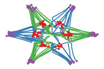
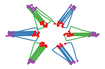
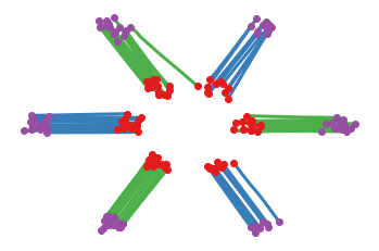
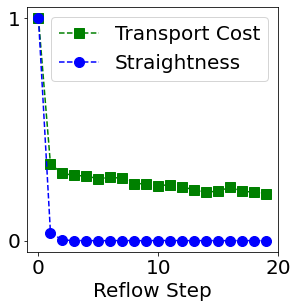
(a)The 1st rectified flow ${\boldsymbol{Z}}^{1}$ ${\boldsymbol{Z}}^{1}=\mathtt{RectFlow}((X_{0},X_{1}))$	(b) Reflow ${\boldsymbol{Z}}^{2}$ ${\boldsymbol{Z}}^{2}=\mathtt{RectFlow}((Z_{0}^{1},Z_{1}^{1}))$	(c) Reflow ${\boldsymbol{Z}}^{3}$ ${\boldsymbol{Z}}^{3}=\mathtt{RectFlow}((Z_{0}^{2},Z_{1}^{2}))$	(d) Transport cost, Straightness

Figure 3: (a)-(c) Samples of trajectories drawn from the reflows on a toy example (${\pi}_{0}$: purple dots, ${\pi}_{1}$: red dots; the green and blue lines are trajectories connecting different modes of ${\pi}_{0},{\pi}_{1}$). (d) The straightness and the relative L2 transport cost v.s. the reflow steps; the values are scaled into $[0,1]$, so 0 corresponds to straight lines and $L_{2}$ optimal transport; see Section 5.1 for more information. We use the non-parametric model in (5) with bandwidth $h=0.1$.

Specifically, we say that a flow $\mathrm{d}Z_{t}=v(Z_{t},t)\mathrm{d}t$ is straight if we have almost surely that $Z_{t}=tZ_{1}+(1-t)Z_{0}$ for $\forall t\in[0,1]$, or equivalently $v(Z_{t},t)=Z_{1}-Z_{0}=const$ following each path. (More precisely, “straight” here refers to straight with a constant speed.) Such straight flows are highly attractive computationally as it is effective a one-step model: a single Euler step update $Z_{1}=Z_{0}+v(Z_{0},0)$ calculates the exact $Z_{1}$ from $Z_{0}$. Note that the linear interpolation ${\boldsymbol{X}}=\{X_{t}\}$ is straight by this definition but it is not a (causal) flow and hence can not be simulated without an oracle assess to draws of both ${\pi}_{0}$ and ${\pi}_{1}$. In comparison, it is non-trivial to make a flow $\mathrm{d}Z_{t}=v(Z_{t},t)\mathrm{d}t$ straight, because if so $v$ must satisfy the inviscid Burgers’ equation $\partial_{t}v+(\partial_{z}v)v=0$:

$$\frac{\mathrm{d}}{\mathrm{d}t}v(Z_{t},t)=\partial_{z}v(Z_{t},t)\dot{Z}_{t}+\partial_{t}v(Z_{t},t)=\partial_{z}v(Z_{t},t)v(Z_{t},t)+\partial_{t}v(Z_{t},t)=0.$$

More generally, we can measure the straightness of any continuously differentiable process ${\boldsymbol{Z}}=\{Z_{t}\}$ by

$$S({\boldsymbol{Z}})=\int_{0}^{1}\mathbb{E}\left[\left\lVert(Z_{1}-Z_{0})-\dot{Z}_{t}\right\rVert^{2}\right]\mathrm{d}t.$$ (3)

$S({\boldsymbol{Z}})=0$ means exact straightness. A flow whose $S({\boldsymbol{Z}})$ is small has nearly straight paths and hence can be simulated accurately using numerical solvers with a small number of discretization steps. Section 3.3 shows that applying rectification recursively provably decreases $S({\boldsymbol{Z}})$ towards zero.

[Theorem 3.7] Let ${\boldsymbol{Z}}^{k}$ be the $k$-th rectified flow induced from $(X_{0},X_{1})$. Then

$$\min_{k\in\{0\cdots K\}}S({\boldsymbol{Z}}^{k})\leq\frac{\mathbb{E}[\left\lVert X_{1}-X_{0}\right\rVert^{2}]}{K}.$$

As shown Figure 1, applying one step of reflow can already provide nearly straight flows that yield good performance when simulated with a single Euler step. It is not recommended to apply too many reflow steps as it may accumulate estimation error on $v^{X}$.

Distillation

After obtaining the $k$-th rectified flow ${\boldsymbol{Z}}^{k}$, we can further improve the inference speed by distilling the relation of $(Z_{0}^{k},Z_{1}^{k})$ into a neural network $\hat{T}$ to directly predict $Z_{1}^{k}$ from $Z_{0}^{k}$ without simulating the flow. Given that the flow is already nearly straight (and hence well approximated by the one-step update), and the distillation can be done efficiently. In particular, if we take $\hat{T}(z_{0})=z_{0}+v(z_{0},0)$, then the loss function for distilling ${\boldsymbol{Z}}^{k}$ is $\mathbb{E}\left[\left\lVert(Z_{1}^{k}-Z_{0}^{k})-v(Z_{0}^{k},0)\right\rVert^{2}\right]$, which is the term in (1) when $t=0$.

We should highlight the difference between distillation and rectification: distillation attempts to faithfully approximate the coupling $(Z_{0}^{k},Z_{1}^{k})$ while rectification yields a different coupling $(Z_{0}^{k+1},Z_{1}^{k+1})$ with lower transport cost and more straight flow. Hence, distillation should be applied only in the final stage when we want to fine-tune the model for fast one-step inference.

On the velocity field $v^{X}$

If $X_{0}$ yields a conditional density function $\rho(x_{0}\leavevmode\nobreak\ |\leavevmode\nobreak\ x_{1})$ when conditioned on $X_{1}=x_{1},$ then the optimal velocity field $v^{X}(z,t)=\mathbb{E}[X_{1}-X_{0}|X_{t}=z]$ can be represented by

$$v^{X}(z,t)=\mathbb{E}\left[\frac{X_{1}-z}{1-t}\eta_{t}(X_{1},z)\right], \eta_{t}(X_{1},z)={\rho\left(\frac{z-tX_{1}}{1-t}\leavevmode\nobreak\ \bigg{|}\leavevmode\nobreak\ X_{1}\right)}\bigg{/}{\mathbb{E}\left[\rho\left(\frac{z-tX_{1}}{1-t}\leavevmode\nobreak\ \bigg{|}\leavevmode\nobreak\ X_{1}\right)\right]},$$ (4)

where the expectation $\mathbb{E}\left[\cdot\right]$ is taken w.r.t. $X_{1}\sim{\pi}_{1}$. This can be seen by noting that $X_{0}=\frac{z-tX_{1}}{1-t}$ and $X_{1}-X_{0}=\frac{X_{1}-z}{1-t}$, when conditioned on $X_{t}=z$. Hence, if $\rho$ is positive and continuous everywhere, then $v^{X}$ is well defined and continuous on $\mathbb{R}^{d}\times[0,1)$. Further, if $\log\eta_{t}$ is continuously differentiable w.r.t. $z$, we can show that

$$\nabla_{z}v^{X}(z,t)=\frac{1}{1-t}\mathbb{E}\left[\left(({X_{1}-z})\nabla_{z}\log\eta_{t}(X_{1},z)-1\right)\eta_{t}(X_{1},z)\right].$$

Note that $\mathrm{d}Z_{t}=v^{X}(Z_{t},t)\mathrm{d}t$ is guaranteed to have a unique solution if $v^{X}$ is uniformly Lipschitz continuous on $[0,a]$ for any $a<1$.

If $X_{0}|X_{1}=x_{1}$ does not yield a conditional density function, $v^{X}(z,t)$ may be undefined or discontinuous, making the ODE $\mathrm{d}Z_{t}=v^{X}(Z_{t},t)\mathrm{d}t$ ill-behaved. A simple fix is to add $X_{0}$ with a Gaussian noise $\xi\sim\mathcal{N}(0,\sigma^{2}I)$ independent of $(X_{0},X_{1})$ to yield a smoothed variable $\tilde{X}_{0}=X_{0}+\xi$, and transfer $\tilde{X}_{0}$ to $X_{1}$ using rectified flow. This would effectively give a randomized mapping of form $T(X_{0}+\xi)$ transporting ${\pi}_{0}$ to ${\pi}_{1}$.

Smooth function approximation

Following (4), we can exactly calculate $v^{X}$ if the conditional density function $\rho(\cdot|x_{1})$ exists and is known, and ${\pi}_{1}$ is the empirical measure of a finite number of points (whose expectation can be evaluated exactly). In this case, running the rectified flow forwardly would precisely recover the points in ${\pi}_{1}$. This, however, is not practically useful in most cases as it completely overfits the data. Hence, it is both necessary and beneficial to fit $v^{X}$ with a smooth function approximator such as neural network or non-parametric models, to obtain smoothed distributions with novel samples that are practically useful.

Deep neural networks are no doubt the best function approximators for large scale problems. For low dimensional problems, the following simple Nadaraya–Watson style non-parametric estimator of $v^{X}$ can yield a good approximation to the exact rectified flow without knowing the conditional density $\rho$:

$$v^{X,h}(z,t)=\mathbb{E}\left[\frac{X_{1}-z}{1-t}\omega_{h}(X_{t},z)\right],$$ (5)

where $\omega_{h}(X_{t},z)=\frac{\kappa_{h}(X_{t},z)}{\mathbb{E}\left[\kappa_{h}(X_{t},z)\right]}$, and $\kappa_{h}(x,z)$ is a smoothing kernel with a bandwith parameter $h>0$ that measures the similarity between $z$ and $x$. Taking the Gaussian RBF kernel $\kappa_{h}(x,z)=\exp(-\left\lVert x-z\right\rVert^{2}/2h^{2})$, then when $h\to 0^{+}$, it can be shown that $v^{X,h}(z,t)$ converges to $v^{X}(z,t)=\mathbb{E}\left[\frac{X_{1}-z}{1-t}\leavevmode\nobreak\ |\leavevmode\nobreak\ X_{t}=z\right]$ on points $z$ that can be attained by $X_{t}$ (i.e., the conditional expectation $\mathbb{E}\left[\cdot\leavevmode\nobreak\ |\leavevmode\nobreak\ X_{t}=z\right]$ exists. ). On points $z$ that $X_{t}$ can not attain, $v^{X,h}(z,t)$ extrapolates the value by finding the $X_{t}$ that is close to $z$. In practice, we replace the expectations in (5) with empirical averaging. We find that $v^{X,h}$ performs well in practice because it is a mixture of linear functions that always point to a point in the support of ${\pi}_{1}$.

2.3 A Nonlinear Extension

We present a nonlinear extension of rectified flow in which the linear interpolation $X_{t}$ is replaced by any time-differentiable curve connecting $X_{0}$ and $X_{1}$. Such generalized rectified flows can still transport ${\pi}_{0}$ to ${\pi}_{1}$ (Theorem 3.3), but no longer guarantee to decrease convex transport costs, or have the straightening effect. Importantly, the method of probability flows [73] and DDIM [70] can be viewed (approximately) as special cases of this framework, allows us to clarify the connection with and the advantages over these methods.

Let ${{\boldsymbol{X}}}=\{X_{t}\colon t\in[0,1]\}$ be any time-differentiable random process that connects $X_{0}$ and $X_{1}$. Let $\dot{X}_{t}$ be the time derivative of $X_{t}$. The (nonlinear) rectified flow induced from ${\boldsymbol{X}}$ is defined as

$$\mathrm{d}Z_{t}=v^{{\boldsymbol{X}}}(Z_{t},t)\mathrm{d}t,\leavevmode\nobreak\ \leavevmode\nobreak\ \leavevmode\nobreak\ \text{with}\leavevmode\nobreak\ \leavevmode\nobreak\ \leavevmode\nobreak\ \leavevmode\nobreak\ Z_{0}=X_{0},\leavevmode\nobreak\ \leavevmode\nobreak\ \leavevmode\nobreak\ \leavevmode\nobreak\ \text{and}\leavevmode\nobreak\ \leavevmode\nobreak\ \leavevmode\nobreak\ \leavevmode\nobreak\ v^{{\boldsymbol{X}}}(z,t)=\mathbb{E}\left[\dot{X}_{t}\leavevmode\nobreak\ |\leavevmode\nobreak\ X_{t}=t\right].$$

We can estimate $v^{{\boldsymbol{X}}}$ by solving

$$\min_{v}\int_{0}^{1}\mathbb{E}\left[w_{t}\left\lVert v(X_{t},\leavevmode\nobreak\ t)-\dot{X}_{t}\right\rVert^{2}\right]\mathrm{d}t,$$ (6)

where $w_{t}\colon(0,1)\to(0,+\infty)$ is a positive weighting sequence ($w_{t}=1$ by default). When using the linear interpolation $X_{t}=tX_{1}+(1-t)X_{0}$, we have $\dot{X}_{t}=X_{1}-X_{0}$ and (6) with $w_{t}=1$ reduces to (1). As we show in Theorem 3.3, the flow ${\boldsymbol{Z}}$ given by this method still preserves the marginal laws of ${\boldsymbol{X}}$, that is, $\mathrm{Law}(Z_{t})=\mathrm{Law}(X_{t})$, $\forall t\in[0,1]$, and hence $(Z_{0},Z_{1})$ remains to be a coupling of ${\pi}_{0},{\pi}_{1}$. However, if ${\boldsymbol{X}}$ is not straight, $(Z_{0},Z_{1})$ no longer guarantees to decrease the convex transport costs over $(X_{0},X_{1})$. More importantly, the reflow procedure no longer straightens the paths of $Z_{t}$.

A simple class of interpolation processes is $X_{t}=\alpha_{t}X_{1}+\beta_{t}X_{0}$ where $\alpha_{t}$ and $\beta_{t}$ are two differentiable sequences that satisfy $\alpha_{1}=\beta_{0}=1$ and $\alpha_{0}=\beta_{1}=0$ to ensure that the process equals $X_{0},X_{1}$ at the starting and end points. In this case, we have $\dot{X}_{t}=\dot{\alpha}_{t}X_{1}+\dot{\beta}_{t}X_{0}$ in (6) where $\dot{\alpha}_{t}$ and $\dot{\beta}_{t}$ are the time derivatives of $\alpha_{t}$ and $\beta_{t}$. The shape of the curve is controlled by the relation of $\alpha_{t}$ and $\beta_{t}$. If we take $\beta_{t}=1-\alpha_{t}$ for all $t$, then $X_{t}$ have straight paths but does not travel at a constant speed; it can be viewed as a time-changed variant of the canonical case $X_{t}=tX_{1}+(1-t)X_{0}$ when $t$ is reparameterized to $\alpha_{t}$. When $\beta_{t}\neq 1-\alpha_{t}$, the paths of $X_{t}$ are not straight lines except some special cases (e.g., $\dot{\alpha}_{t}X_{1}=0$ or $\dot{\beta}_{t}X_{0}=0$, or $X_{1}=aX_{1}$ for some $a\in\mathbb{R}$).

2.3.1 Probability Flow ODEs and DDIM

The probability flow ODEs (PF-ODEs) [73] and denoising diffusion implicit models (DDIM) [70] are methods for learning ODE-based generative models of ${\pi}_{1}$ from a spherical Gaussian initial distribution ${\pi}_{0}$, derived by converting a SDE learned by denoising diffusion methods to an ODE with equivalent marginal laws. In [73], three types of PF-ODEs are derived from three types of SDEs learned as score-based generative models, including variance-exploding (VE) SDE, variance-preserving (VP) SDE, and sub-VP SDE, which we denote by VE ODE, VP ODE, and sub-VP ODE, respectively. VP ODE is equivalent to the continuous time limit of DDIM, which is derived from the denoising diffusion probability model (DDPM) [23]. As the derivations of PF-ODEs and DDIM require advanced tools in stochastic calculus, we limit our discussion on the final algorithmic procedures suggested in [73, 23], which we summarize in Section 3.5. The readers are referred to [73, 70] for the details.

[Proposition 3.11] All variants of PF-ODEs can be viewed as instances of (6) when using $X_{t}=\alpha_{t}X_{1}+\beta_{t}\xi$ for some $\alpha_{t},\beta_{t}$ with $\alpha_{1}=1,\beta_{1}=0$, where $\xi\sim\mathcal{N}(0,I)$ is a standard Gaussian random variable.

Here we need to use introduce $\xi$ to replace $X_{0}$ because the choices of $\alpha_{t}$ and $\beta_{t}$ suggested in [73, 70, 23] do not satisfy the boundary condition of $\alpha_{0}=0$ and $\beta_{0}=1$ at $t=0$, and hence $X_{0}\neq\xi$. Instead, in these methods, the initial distribution $X_{0}\sim{\pi}_{0}$ is implicitly defined as $X_{0}=\alpha_{0}X_{1}+\beta_{0}\xi$, which is approximated by $X_{0}\approx\beta_{0}\xi$ by making $\alpha_{0}X_{1}\ll\beta_{0}\xi$. Hence, ${\pi}_{0}$ is set to be $\mathcal{N}(0,\beta_{0}^{2}I)$ in these methods. Viewed through our framework, there is no reason to restrict $\xi$ to be $\mathcal{N}(0,\beta_{0}^{2}I)$, or not set $\alpha_{0}=0,\beta_{0}=1$ to avoid the approximation.

Rectified flow	VP ODE	sub-VP ODE
($\alpha_{t}=t$, $\beta_{t}=1-t$)	($\alpha_{t}$ in (7), $\beta_{t}=\sqrt{1-\alpha_{t}^{2}}$)	($\alpha_{t}$ in (7), $\beta_{t}={1-\alpha_{t}^{2}}$)
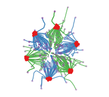
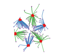
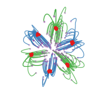
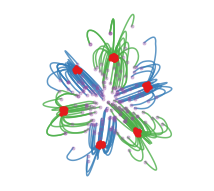
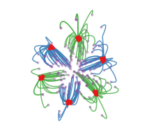
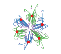
1-Rectified Flow 2-Rectified Flow	1-Rectified Flow 2-Rectified Flow	1-Rectified Flow 2-Rectified Flow

Figure 4: Comparing rectified flow with VP ODE and sub-VP ODE when ${\pi}_{0}=\mathcal{N}(0,I)$ (purple dots) and ${\pi}_{1}$ is a low variance Gaussian mixture shown as the red dots. The linear rectified flow yields nearly straight trajectories with one step of reflow. But the trajectories of VP ODE and sub-VP ODE are curved and can not be straightened by reflowing.

Time-Discretization	Rectified Flow	VP ODE	sub-VP ODE	VP ODE (const speed)
Steps $N$	$\alpha_{t}=t,\beta_{t}=1-t$	$\alpha_{t}$ in (7), $\beta_{t}=\sqrt{1-\alpha_{t}^{2}}$	$\alpha_{t}$ in (7), $\beta_{t}={1-\alpha_{t}^{2}}$	$\alpha_{t}=t$, $\beta_{t}=\sqrt{1-\alpha_{t}^{2}}$
$N=1$
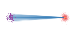
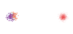
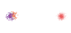
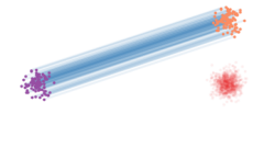
$N=2$
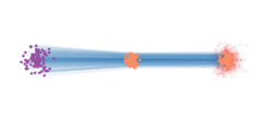
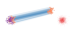
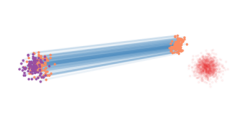
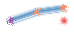
$N=5$
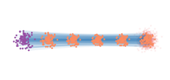
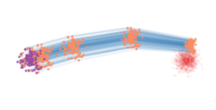
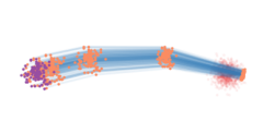
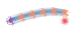
$N=100$

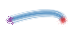
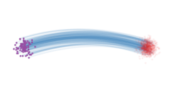
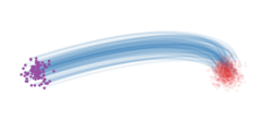
Figure 5: Trajectories of different methods when varying the number of discretization steps $N$ (purple dots: ${\pi}_{0}$; red dots: ${\pi}_{1}$; orangle dots: intermediate steps; blue curves: flow trajectories). The rectified flow travels in straight lines and progresses uniformly in time; it generates the mean of ${\pi}_{1}$ when simulated with a single Euler step, and quickly covers the whole distribution ${\pi}_{1}$ with more steps (in this case $N=2$ is sufficient). In comparison, VP ODE and sub-VP ODE travel in curves with non-uniform speed: they tend to be slow in the beginning and speed up in the later phase (much of the update happens when $t{\scriptstyle\gtrapprox}0.5$). The non-uniform speed can be avoided by setting $\alpha_{t}=t$ (see the last column).

VP ODE and sub-VP ODE

The VP ODE and sub-VP ODE of [73] use the following shared $\alpha_{t}$:

$$\text{(sub-)VP ODE:}\leavevmode\nobreak\ \leavevmode\nobreak\ \leavevmode\nobreak\ \leavevmode\nobreak\ \alpha_{t}=\exp\left(-\frac{1}{4}a(1-t)^{2}-\frac{1}{2}b(1-t)\right); a=19.9 b=0.1$$ default values: , , (7)

where the default values of $a,b$ are chosen to match the continuous time limit of the shared training procedure of DDIM and DDPM. The difference of VP ODE and sub-VP ODE is on the choice of $\beta_{t}$, given as follows:

$$\text{VP ODE:\leavevmode\nobreak\ \leavevmode\nobreak\ \leavevmode\nobreak\ }\beta_{t}=\sqrt{1-\alpha_{t}^{2}}, \text{sub-VP ODE:\leavevmode\nobreak\ \leavevmode\nobreak\ \leavevmode\nobreak\ }\beta_{t}={1-\alpha_{t}^{2}}.$$ (8)

As $\beta_{0}\approx 1$ in both VP and sub-VP ODE, the ${\pi}_{0}$ in both cases are taken as $\mathcal{N}(0,I)$.

The choices of $\alpha_{t},\beta_{t}$ above are the consequence of the SDE-based derivation in [73]. However, they are not well-motivated when we exam the path properties of the induced ODEs:

$\bullet$ Non-straight paths: Due to choices of $\beta_{t}$ in (8), the trajectories of VP ODE and sub-VP ODE are curved in general, and can not be straightened by the reflow procedure. We should choose $\beta_{t}=1-\alpha_{t}$ to induce straight paths.

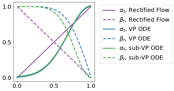
Figure 6: $t$ vs. $\alpha_{t},\beta_{t}$ of different methods.

$\bullet$ Non-uniform speed: The exponential form of $\alpha_{t}$ in (7) is a consequence of using Ornstein–Uhlenbeck processes in the derivation of SDE models [73, 23]. However, there is no clear advantage of using (7) for ODEs. As shown in Figure 5, the $\alpha_{t}$ and $\beta_{t}$ of VP and sub-VP ODE change slowly in the early phase ($t{\scriptstyle\lessapprox}0.5$). As a result, the flow also moves slowly in beginning and hence most of the updates are concentrated in the later phase. Such non-uniform update speed, in addition to the non-straight paths, make VP ODE and sub-VP ODE perform sub-optimally when using large step sizes, even for transport between simple spherical Gaussian distributions (see Figure 5). As we show in the last column of Figure 5, changing the exponential $\alpha_{t}$ to the linear function $\alpha_{t}=t$ in VP ODE allows us to get a uniform update speed while preserving the same continuous-time trajectories.

VE ODE

The VE ODE of [73] uses $\alpha_{t}=1$ and $\beta_{t}=\sigma_{\min}\sqrt{r^{2(1-t)}-1}$ where $\sigma_{\min}=0.01$ by default $r$ is set such that $\sigma_{\max}\coloneqq r\sigma_{\min}$ is as large as the maximum Euclidean distance between all pairs of training data points from ${\pi}_{1}$ (Technique 1 of [72]). Assume that $\sigma_{\max}^{2}$ is much larger than both $\sigma_{\min}^{2}$ and the variance of $X_{1}$, then $X_{0}=X_{1}+\beta_{0}\xi\approx\sigma_{\max}\xi$, and we can set the initial distribution to be ${\pi}_{0}\sim\mathcal{N}(0,\sigma_{\max}^{2}I)$, which has much larger variance than ${\pi}_{1}$. Hence, VE ODE can not be applied to (and not shown in) the toys in Figure 4 and Figure 5. As the case of (sub-)VP ODE, the restriction on $\xi$ is in fact unnecessary and requirement that $\sigma_{\max}$ is unnatural viewed from our framework. On the other hand, the trajectories of $X_{t}$ in VE ODE are indeed straight lines, because the direction of $\dot{X}_{t}=\dot{\beta}_{t}\xi$ is always the same as $\xi$. However, the choice of $\beta_{t}$ causes a non-uniform speed issue similar to that of (sub-)VP ODE.

Following [73, 23], a line of works have been proposed to improve the choices of $\alpha_{t},\beta_{t}$, but remain to be constrained by the basic design space from the SDE-to-ODE derivation; see for example [54, 29, 95].

To summarize, the simple nonlinear rectified flow framework in (6) both simplifies and extends the existing framework, and sheds a number of importance insights:

$\bullet$ Learning ODEs can be considered directly and independently without resorting to diffusion/SDE methods;

$\bullet$ The paths of the learned ODEs can be specified by any smooth interpolation curve $X_{t}$ of $X_{0}$ and $X_{1}$;

$\bullet$ The initial distribution ${\pi}_{0}$ can be chosen arbitrarily, independent with the choice of the interpolation $X_{t}$.

$\bullet$ The canonical linear interpolation $X_{t}=tX_{1}+(1-t)X_{0}$ should be recommended as a default choice.

On the other hand, non-linear choices of $X_{t}$ can be useful when we want to incorporate certain non-Euclidan geometry structure of the variable, or want to place certain constraints on the trajectories of the ODEs. We leave this for future works.

3 Theoretical Analysis

We present the theoretical analysis for rectified flow. The results are summarized as follows.

$\bullet$ [Section 3.1] All nonlinear rectified flows with any interpolation $X_{t}$ preserve the marginal laws.

$\bullet$ [Section 3.2] The rectified flow (with the canonical linear interpolation) reduces convex transport costs.

$\bullet$ [Section 3.3] Reflow guarantees to straighten the (linear) rectified flows.

$\bullet$ [Section 3.4] We clarify the relation between straight couplings and $c$-optimal couplings.

$\bullet$ [Section 3.5] We establish PF-ODEs as instances of nonlinear rectified flows.

3.1 The Marginal Preserving Property

The marginal preserving property that $\mathrm{Law}(Z_{t})=\mathrm{Law}(X_{t})$ for $\forall t$ is a general property of the nonlinear rectified flows in (6), regardless whether the interpolation $X_{t}$ is straight or not.

Definition 3.1.

For a path-wise continuously differentiable random process ${{\boldsymbol{X}}}=\{X_{t}\colon t\in[0,1]\}$, its expected velocity $v^{{\boldsymbol{X}}}$ is defined as

$$v^{{\boldsymbol{X}}}(x,t)=\mathbb{E}[\dot{X}_{t}\leavevmode\nobreak\ |\leavevmode\nobreak\ X_{t}=x],\leavevmode\nobreak\ \leavevmode\nobreak\ \leavevmode\nobreak\ \leavevmode\nobreak\ \leavevmode\nobreak\ \forall x\in\mathrm{supp}(X_{t}).$$

For $x\not\in\mathrm{supp}(X_{t})$, the conditional expectation is not defined and we set $v^{{\boldsymbol{X}}}$ arbitrarily, say $v^{{\boldsymbol{X}}}(x,t)=0$.

Definition 3.2.

We call that ${\boldsymbol{X}}$ is rectifiable if $v^{{\boldsymbol{X}}}$ is locally bounded and the solution of the integral equation below exists and is unique:

$$Z_{t}=Z_{0}+\int_{0}^{t}v^{{\boldsymbol{X}}}(Z_{t},t)\mathrm{d}t,\leavevmode\nobreak\ \leavevmode\nobreak\ \leavevmode\nobreak\ \leavevmode\nobreak\ \forall t\in[0,1],\leavevmode\nobreak\ \leavevmode\nobreak\ \leavevmode\nobreak\ \leavevmode\nobreak\ Z_{0}=X_{0}.$$ (9)

In this case, ${\boldsymbol{Z}}=\{Z_{t}\colon t\in[0,1]\}$ is called the rectified flow induced from ${\boldsymbol{X}}$.

Theorem 3.3.

Assume ${\boldsymbol{X}}$ is rectifiable and ${\boldsymbol{Z}}$ is its rectified flow. Then $\mathrm{Law}(Z_{t})=\mathrm{Law}(X_{t})$ for $\forall t\in[0,1]$.

Proof.

For any compactly supported continuously differentiable test function $h\colon\mathbb{R}^{d}\to\mathbb{R}$, we have

$$\frac{\mathrm{d}}{\mathrm{d}t}\mathbb{E}[h(X_{t})]=\mathbb{E}[\nabla h(X_{t})^{\top}\dot{X}_{t}]=\mathbb{E}[\nabla h(X_{t})^{\top}v^{{\boldsymbol{X}}}(X_{t},t)],$$ (10)

where we used $v^{{\boldsymbol{X}}}(X_{t},t)=\mathbb{E}[\dot{X}_{t}|X_{t}]$. By definition, this is equivalent to that ${\pi}_{t}\coloneqq\mathrm{Law}(X_{t})$ solves in the sense of distributions the continuity equation with drift $v_{t}^{{\boldsymbol{X}}}\coloneqq v^{{\boldsymbol{X}}}(\cdot,t)$:

$$\dot{\pi}_{t}+\nabla\cdot(v_{t}^{{\boldsymbol{X}}}{\pi}_{t})=0.$$ (11)

To see the equivalence of (10) and (11), we can multiply (11) with $h$ and integrate both sides:

$$0=\int h(\dot{\pi}_{t}+\nabla\cdot(v_{t}^{{\boldsymbol{X}}}{\pi}_{t}))=\int h\dot{\pi}_{t}-\nabla h^{\top}v_{t}^{{\boldsymbol{X}}}{\pi}_{t}=\frac{\mathrm{d}}{\mathrm{d}t}\mathbb{E}[h(X_{t})]-\mathbb{E}[\nabla h(X_{t})^{\top}v^{{\boldsymbol{X}}}(X_{t},t)],$$

where we use integration by parts that $\int h\nabla\cdot(v^{{\boldsymbol{X}}}_{t}{\pi}_{t})=-\int\nabla h^{\top}(v^{{\boldsymbol{X}}}_{t}{\pi}_{t})$.

Because $Z_{t}$ is driven by the same velocity field $v^{{\boldsymbol{X}}}$, its marginal law $\mathrm{Law}(Z_{t})$ solves the very same equation with the same initial condition ($Z_{0}=X_{0}$). Hence, the equivalence of $\mathrm{Law}(Z_{t})$ and $\mathrm{Law}(X_{t})$ follows if the solution of (11) is unique, which is equivalent to the uniqueness of the solution of $\mathrm{d}Z_{t}=v^{{\boldsymbol{X}}}(Z_{t},t)$ following Corollary 1.3 of Kurtz [37] (see also Theorem 4.1 of Ambrosio and Crippa [1]). ∎

3.2 Reducing Convex Transport Costs

The fact that $(Z_{0},Z_{1})$ yields no larger convex transport costs than $(X_{0},X_{1})$ is a consequence of using the special linear interpolation $X_{t}=tX_{1}+(1-t)X_{0}$ as the geodesic of Euclidean space.

Definition 3.4.

A coupling $(X_{0},X_{1})$ is called rectifiable if its linear interpolation process ${\boldsymbol{X}}=\{tX_{1}+(1-t)X_{0}\colon t\in[0,1]\}$ is rectifiable. In this case, the ${\boldsymbol{Z}}=\{Z_{t}\colon t\in[0,1]\}$ in (9) is called the rectified flow of coupling $(X_{0},X_{1})$, denoted as ${\boldsymbol{Z}}=\mathtt{RectFlow}((X_{0},X_{1}))$, and $(Z_{0},Z_{1})$ is called the rectified coupling of $(X_{0},X_{1})$, denoted as $(Z_{0},Z_{1})=\mathtt{Rectify}((X_{0},X_{1})).$

Theorem 3.5.

Assume $(X_{0},X_{1})$ is rectifiable and $(Z_{0},Z_{1})=\mathtt{Rectify}((X_{0},X_{1}))$. Then for any convex function $c\colon\mathbb{R}^{d}\to\mathbb{R}$, we have

$$\mathbb{E}[c(Z_{1}-Z_{0})]\leq\mathbb{E}[c(X_{1}-X_{0})].$$

Proof.

The proof is based on elementary applications of Jensen’s inequality.

$$\mathbb{E}\left[c(Z_{1}-Z_{0})\right] =\mathbb{E}\left[c\left(\int_{0}^{1}v^{{\boldsymbol{X}}}(Z_{t},t)\mathrm{d}t\right)\right]\leavevmode\nobreak\ \leavevmode\nobreak\ \leavevmode\nobreak\ \leavevmode\nobreak\ \leavevmode\nobreak\ \leavevmode\nobreak\ \leavevmode\nobreak\ \text{{\color[rgb]{1,0,1}//as $\mathrm{d}Z_{t}=v^{{\boldsymbol{X}}}(Z_{t},t)\mathrm{d}t$}}$$

$$\leq\mathbb{E}\left[\int_{0}^{1}c\left(v^{{\boldsymbol{X}}}(Z_{t},t)\right)\mathrm{d}t\right]\leavevmode\nobreak\ \leavevmode\nobreak\ \leavevmode\nobreak\ \leavevmode\nobreak\ \leavevmode\nobreak\ \leavevmode\nobreak\ \leavevmode\nobreak\ \text{{\color[rgb]{1,0,1}//convexity of $c$, Jensen's inequality}}$$

$$=\mathbb{E}\left[\int_{0}^{1}c\left(v^{{\boldsymbol{X}}}(X_{t},t)\right)\mathrm{d}t\right]\leavevmode\nobreak\ \leavevmode\nobreak\ \leavevmode\nobreak\ \leavevmode\nobreak\ \leavevmode\nobreak\ \leavevmode\nobreak\ \leavevmode\nobreak\ \text{{\color[rgb]{1,0,1}//$X_{t}$ and $Z_{t}$ shares the same marginals}}$$

$$=\mathbb{E}\left[\int_{0}^{1}c\left(\mathbb{E}\left[(X_{1}-X_{0})\leavevmode\nobreak\ |\leavevmode\nobreak\ X_{t}\right]\right)\mathrm{d}t\right]\leavevmode\nobreak\ \leavevmode\nobreak\ \leavevmode\nobreak\ \leavevmode\nobreak\ \leavevmode\nobreak\ \leavevmode\nobreak\ \leavevmode\nobreak\ \text{{\color[rgb]{1,0,1}//definition of $v^{{\boldsymbol{X}}}$}}$$

$$\leq\mathbb{E}\left[\int_{0}^{1}\mathbb{E}\left[c\left(X_{1}-X_{0}\right)|\leavevmode\nobreak\ X_{t}\right]\mathrm{d}t\right]\leavevmode\nobreak\ \leavevmode\nobreak\ \leavevmode\nobreak\ \leavevmode\nobreak\ \leavevmode\nobreak\ \leavevmode\nobreak\ \leavevmode\nobreak\ \text{{\color[rgb]{1,0,1}//convexity of $c$, Jensen's inequality}}$$

$$=\int_{0}^{1}\mathbb{E}\left[c\left(X_{1}-X_{0}\right)\right]\mathrm{d}t\leavevmode\nobreak\ \leavevmode\nobreak\ \leavevmode\nobreak\ \leavevmode\nobreak\ \leavevmode\nobreak\ \leavevmode\nobreak\ \leavevmode\nobreak\ \text{{\color[rgb]{1,0,1}//$\mathbb{E}[\mathbb{E}[(X_{1}-X_{0})|X_{t}]]=\mathbb{E}[(X_{1}-X_{0})]$}}$$

$$=\mathbb{E}\left[c\left(X_{1}-X_{0}\right)\right].$$

∎

If $X_{t}$ is straight but with positive non-constant speed, that is, $X_{t}=\alpha_{t}X_{1}+\beta_{t}X_{0}$ with $\beta_{t}=1-\alpha_{t}$ and $\dot{\alpha}_{t}\geq 0$, then we still have $\mathbb{E}[c(Z_{1}-Z_{0})]\leq\mathbb{E}[c(X_{1}-X_{0})]$ if $c$ is convex and $m$-homogeneous in that $c(ax)=\left\lvert a\right\rvert^{m}c(x)$ for $\forall a\in\mathbb{R},x\in\mathbb{R}^{d}$, with some constant $m\in(0,1]$.

3.3 The Straightening Effect

A coupling $(X_{0},X_{1})$ is said to be straight (or fully rectified) if it is a fixed point of the $\mathtt{Rectify}(\cdot)$ mapping. It is desirable to obtain a straight coupling because its rectified flow is straight and hence can be simulated exactly with one step using numerical solvers. In this section, we first characterize the basic properties of straight couplings, showing that a coupling is straight iff its linear interpolation paths do not intersect with each other. Then, we prove that recursive rectification straightens the coupling and its related flow with a ${O}{\left(1/k\right)}$ rate, where $k$ is the number of rectification steps.

Theorem 3.6.

Assume $(X_{0},X_{1})$ is rectifiable. Let $X_{t}=tX_{1}+(1-t)X_{0}$ and ${\boldsymbol{Z}}=\mathtt{RectFlow}((X_{0},X_{1}))$. Then $(X_{0},X_{1})$ is a straight coupling iff the following equivalent statements hold.

1. There exists a strictly convex function $c\colon\mathbb{R}^{d}\to\mathbb{R}$, such that $\mathbb{E}[c(Z_{1}-Z_{0})]=\mathbb{E}[c(X_{1}-X_{0})]$.

2. $(X_{0},X_{1})$ is a fixed point of $\mathtt{Rectify}(\cdot)$, that is, $(X_{0},X_{1})=(Z_{0},Z_{1})$.

3. The rectified flow coincides with the linear interpolation process: ${\boldsymbol{X}}={\boldsymbol{Z}}$.

4. The paths of the linear interpolation ${\boldsymbol{X}}$ do not intersect:

   $$V((X_{0},X_{1})):=\int_{0}^{1}\mathbb{E}\left[\left\lVert X_{1}-X_{0}-\mathbb{E}\left[X_{1}-X_{0}\leavevmode\nobreak\ |\leavevmode\nobreak\ X_{t}\right]\right\rVert^{2}\right]\mathrm{d}t=0,$$ (12)

   where $V((X_{0},X_{1}))=0$ indicates that $X_{1}-X_{0}=\mathbb{E}[X_{1}-X_{0}|X_{t}]$ almost surely when $t\sim\textrm{Uniform}([0,1])$, meaning that the lines passing through each $X_{t}$ is unique, and hence no linear interpolation paths intersect.

Proof.

$3\to 2\to 1$: Obvious.

$1\to 4$: If $\mathbb{E}[c(Z_{1}-Z_{0})]=\mathbb{E}[c(X_{1}-X_{0})]$, the two applications of Jensen’s inequality in the proof of Theorem 3.5 are tight. Because $c$ is strictly convex, the second Jensen’s inequality in the proof implies that $X_{1}-X_{0}=\mathbb{E}[X_{1}-X_{0}\leavevmode\nobreak\ |\leavevmode\nobreak\ X_{t}]$ almost surely w.r.t. $X$ and $t\sim\textrm{Uniform}([0,1]),$ which implies that $V({\boldsymbol{X}})=0.$

$4\to 3$: If $V({\boldsymbol{X}})=0$, we have $\int_{0}^{s}(X_{1}-X_{0})\mathrm{d}t=\int_{0}^{s}\mathbb{E}[X_{1}-X_{0}|X_{t}]\mathrm{d}t=\int_{0}^{s}v^{X}(X_{t},t)\mathrm{d}t$ for $s\in(0,1]$. Hence

$$X_{t}=X_{0}+\int_{0}^{t}(X_{1}-X_{0})\mathrm{d}t=X_{0}+\int_{0}^{t}v^{X}(X_{t},t)\mathrm{d}t.$$

Because ${\boldsymbol{Z}}$ satisfies the same equation (9), we have ${\boldsymbol{X}}={\boldsymbol{Z}}$ by the uniqueness of the solution.

∎

${O}{\left(1/K\right)}$ convergence rate

We now show that as we apply rectification recursively, the rectified flows become increasingly straight and the linear interpolation of the couplings becomes increasingly non-intersecting.

Theorem 3.7.

Let ${\boldsymbol{Z}}^{k}$ the $k$-th rectified flow of $(X_{0},X_{1})$, that is, ${\boldsymbol{Z}}^{k+1}=\mathtt{RectFlow}((Z_{0}^{k},Z_{1}^{k}))$ and $(Z_{0}^{0},Z_{1}^{0})=(X_{0},X_{1})$. Assume each $(Z_{0}^{k},Z_{1}^{k})$ is rectifiable for $k=0,\ldots,K$.

Then

$$\sum_{k=0}^{K}S({\boldsymbol{Z}}^{k+1})+V((Z^{k}_{0},Z^{k}_{1}))\leq\mathbb{E}\left[\left\lVert X_{1}-X_{0}\right\rVert^{2}\right].$$

Hence, $\mathbb{E}[\left\lVert X_{1}-X_{0}\right\rVert^{2}]<+\infty$, we have $\min_{k\leq K}(S({\boldsymbol{Z}}^{k})+V((Z_{0}^{k},Z_{1}^{k}))={O}{\left(1/K\right)}$.

Proof.

Taking $c(x)=\left\lVert x\right\rVert^{2}$ in the proof of Theorem 3.5, we can obtain that

$$\mathbb{E}\left[\left\lVert X_{1}-X_{0}\right\rVert\right]-\mathbb{E}\left[\left\lVert Z_{1}-Z_{0}\right\rVert\right]=S({\boldsymbol{Z}})+V((X_{0},X_{1})).$$ (13)

Applying it to each rectification step yields

$$\mathbb{E}\left[\left\lVert Z^{k}_{1}-Z^{k}_{0}\right\rVert^{2}\right]-\mathbb{E}\left[\left\lVert Z^{k+1}_{1}-Z^{k+1}_{0}\right\rVert^{2}\right]=S({\boldsymbol{Z}}^{k+1})+V((Z_{0}^{k},Z_{1}^{k})).$$

A telescoping sum on $k=0,\ldots,K$ gives the result.

∎

3.4 Straight vs. Optimal Couplings

A coupling $(X_{0},X_{1})$ is called $c$-optimal if it achieves the minimum of $\mathbb{E}[c(X_{1}-X_{0})]$ among all couplings that share the same marginals. Understanding and computing the optimal couplings have been the main focus of optimal transport [e.g., 84, 2, 15, 59]. Straight couplings is a different desirable property. In the following, we show that straightness is a necessary but not sufficient condition of being $c$-optimal for a strictly convex function $c$, except in the one dimensional case when the two concepts coincides. Hence, it is “easier” to find a straight coupling than a $c$-optimal couplings.

Theorem 3.8.

If a rectifiable coupling $(X_{0},X_{1})$ is $c$-optimal for some strictly convex cost function $c$, then $(X_{0},X_{1})$ is a straight coupling.

Proof.

Let $(Z_{0},Z_{1})=\mathtt{Rectify}((X_{0},X_{1}))$. If $(X_{0},X_{1})$ is $c$-optimal, we must have $\mathbb{E}[c(Z_{1}-Z_{0})]=\mathbb{E}[c(X_{1}-X_{0})]$. This implies Statement 1 in Theorem 3.6 and hence that $(X_{0},X_{1})$ is straight. ∎

1D Case

For any ${\pi}_{0},{\pi}_{1}$ on $\mathbb{R}$, there exists an unique coupling $(X_{0}^{*},X_{1}^{*})$ that is simultaneously optimal for all non-negative convex cost functions $c$. This coupling is uniquely characterized by a monotonic property: for every $(x_{0},x_{1})$ and $(x_{0}^{\prime},x_{1}^{\prime})$ in the support of $(X_{0}^{*},X_{1}^{*})$, if $x_{0}<x_{0}^{\prime}$, then $x_{1}\leq x_{1}^{\prime}$. Furthermore, if ${\pi}_{0}$ is absolutely continuously w.r.t. the Lebesgue measure, then $(X_{0}^{*},X_{1}^{*})$ must be deterministic in that there exists a mapping $T\colon\mathbb{R}\to\mathbb{R}$ such that $X_{1}^{*}=T(X_{0}^{*})$. See [65].

In the following, we show that straight couplings on $\mathbb{R}$ coincides with the deterministic monotonic coupling $(X_{0}^{*},X_{1}^{*})$ and hence is unique and simultaneously optimal for all convex $c$ when ${\pi}_{0}$ is absolutely continuous. The idea is that, in $\mathbb{R}$, a coupling is monotonic iff its linear interpolation paths do not intersect, a characteristic feature of straight couplings.

Lemma 3.9.

A coupling on $\mathbb{R}$ is straight iff it is deterministic and monotonic.

Theorem 3.10.

For any ${\pi}_{0},{\pi}_{1}$ on $\mathbb{R}$, there exists either no straight coupling, or a unique straight coupling. Further, if exists, the unique straight coupling is deterministic and monotonic, and jointly optimal w.r.t. all convex cost functions $c\colon\mathbb{R}^{d}\to[0,+\infty)$ for which the minimum value of $\mathbb{E}\left[c(X_{1}-X_{0})\right]$ exists and is finite.

Proof of Lemma 3.9.

If $(X_{0},X_{1})$ on $\mathbb{R}$ is straight, then it coincides with its rectified coupling $(Z_{0},Z_{1})=\mathtt{Rectify}((X_{0},X_{1})).$ But because $(Z_{0},Z_{1})$ is induced from the rectified flow $\mathrm{d}Z_{t}=v^{X}(Z_{t},t)\mathrm{d}t$, it is obviously deterministic. It is also monotonic due to the non-crossing property of flows. Specifically, if $(Z_{0},Z_{1})$ is not monotonic, there exists $(z_{0},z_{1})$ and $(z_{0}^{\prime},z_{1}^{\prime})$ in the support of $(Z_{0},Z_{1})$ such that $z_{0}<z_{0}^{\prime}$ and $z_{1}>z_{1}^{\prime}$. If this happens, there must exists $t_{0}\in(0,1)$, such that $z_{t_{0}}=z_{t_{0}}^{\prime}$. But by the uniqueness of the solution, we have $z_{t}=z_{t}$ for $t\geq t_{0}$, which is conflicting with $z_{1}>z_{1}^{\prime}$.

Assume $(X_{0},X_{1})$ is deterministic and monotonic. Due to the monotonicity, there exists no $x_{0}$ and $x_{0}^{\prime}$ in the support of ${\pi}_{0}$, such that $x_{0}\neq x_{0}^{\prime}$ and $x_{t_{0}}=x_{t_{0}}^{\prime}$ for some $t_{0}<1$. This suggests that $X_{1}-X_{0}=\mathbb{E}[X_{1}-X_{0}\leavevmode\nobreak\ |\leavevmode\nobreak\ X_{t}]=v^{X}(X_{t},t)$ for $t\in(0,1)$, and hence $\mathrm{d}X_{t}=(X_{1}-X_{0})\mathrm{d}t=v^{X}(X_{t})\mathrm{d}t$, which is the ODE of the rectified flow. In addition, $X_{t}$ is obviously the unique solution of this ODE. Hence $(X_{0},X_{1})$ is rectifiable and straight following Statement 3 of Theorem 3.6. ∎

Proof of Theorem 3.10.

This is the result of Lemma 3.9 combined with the fact that the monotonic coupling is unique and jointly optimal for all convex $c$ for which the optimal coupling exists, following Lemma 2.8 and Theorem 2.9 of [65]. ∎

Multi-dimensional cases

On the other hand, on $\mathbb{R}^{d}$ with $d\geq 2$, the different cost functions $c$ do not share a common optimal coupling in general, and a straight coupling is not guaranteed to optimize a specific $c$; this is expected because the $\mathtt{Rectify}(\cdot)$ procedure does not depend on a particular choice of $c$. Hence, one must modify the $\mathtt{Rectify}(\cdot)$ procedure to tailor it to a specific $c$ of interest.

In a recent work [30], it was conjectured that the couplings $(Z_{0},Z_{1})$ induced from VP ODE (equivalently DDIM) yields an optimal coupling w.r.t. the quadratic loss, which was proved to be false in [39, 78]. Here we show that even straight couplings are not guaranteed to be optimal, not to mention that VP ODE does not follow straight paths by design.

We explore this in a separate work [42] that is devoted to modifying rectified flow to find $c$-optimal couplings; a result from [42] that can be easily stated is that the optimal coupling w.r.t. the quadratic cost $c(\cdot)=\left\lVert\cdot\right\rVert^{2}$ can be achieved as the fixed point of $\mathtt{Rectify}(\cdot)$ if $v$ is restricted to be a gradient field of form $v(x,t)=\nabla f(x,t)$ when solving (1). Restricting $v$ to be a gradient field removes the rotational component of the velocity field $v^{{\boldsymbol{X}}}$ that causes sub-optimal transport cost.

3.5 Denoising Diffusion Models and Probability Flow ODEs

We prove that the probability flow ODEs (PF-ODEs) of [73] can be viewed as nonlinear rectified flows in (6) with $X_{t}=\alpha_{t}X_{1}+\beta_{t}\xi.$ We start with introducing the algorithmic procedures of the denoising diffusion models and PF-ODEs, and refer the readers to the original works [73, 23, 70] for the theoretical derivations.

The denoising diffusion methods learn to generative models by constructing an SDE model driven by a standard Brownian motion $W_{t}$:

$$\mathrm{d}U_{t}=b(U_{t},t)\mathrm{d}t+\sigma_{t}\mathrm{d}W_{t},\leavevmode\nobreak\ \leavevmode\nobreak\ \leavevmode\nobreak\ U_{0}\sim{\pi}_{0},$$ (14)

where $\sigma_{t}\colon[0,1]\to[0,+\infty)$ is a (typically) fixed diffusion coefficient, $b$ is a trainable neural network, and the initial distribution ${\pi}_{0}$ is restricted to a spherical Gaussian distribution determined by hyper-parameter setting of the algorithm. The idea is to first collapse the data into an (approximate) Gaussian distribution using a diffusion process, mostly an Ornstein-Uhlenbeck (OU) process, and then estimate the generative diffusion process (14) as the time reversal [e.g., 3] of the collapsing process.

Without diving into the derivations, the training loss of the VE, VP, sub-VP SDEs for $b$ in [73] can be summarized as follows:

$$\min_{v}\int_{0}^{1}\mathbb{E}\left[w_{t}\left\lVert v(V_{t},t)-Y_{t}\right\rVert^{2}_{2}\right]\mathrm{d}t, V_{t}=\alpha_{t}X_{1}+\beta_{t}\xi_{t}, Y_{t}=-\eta_{t}V_{t}-\frac{\sigma_{t}^{2}}{\beta_{t}}\xi_{t},$$ (15)

where $\xi_{t}$ is a diffusion process satisfying $\xi_{t}\sim\mathcal{N}(0,I)$, and $\eta_{t},\sigma_{t}$ are the hyper-parameter sequences of the algorithm, and $\alpha_{t},\beta_{t}$ are determined by $\eta_{t},\sigma_{t}$ via

$$\alpha_{t}=\exp\left(\int_{t}^{1}\eta_{s}\mathrm{d}s\right),\leavevmode\nobreak\ \leavevmode\nobreak\ \leavevmode\nobreak\ \leavevmode\nobreak\ \leavevmode\nobreak\ \beta_{t}^{2}=\int_{t}^{1}\exp\left(2\int_{t}^{s}\eta_{r}\mathrm{d}r\right)\sigma_{s}^{2}\mathrm{d}s.$$ (16)

The relation in (16) is derived to make $\tilde{V}_{t}=V_{1-t}=\alpha_{1-t}X_{1}+\beta_{1-t}\xi_{t}$ follow the Ornstein-Uhlenbeck (OU) processes $\mathrm{d}\tilde{V}_{t}=\eta_{1-t}\tilde{V}_{t}\mathrm{d}t+\sigma_{1-t}\mathrm{d}W_{t}$.

VE SDE, which is equivalent to SMLD in [71, 72], takes $\eta_{t}=0$ and hence has $\alpha_{t}=1$. (sub-)VP SDE takes $\eta_{s}$ to be a linear function of $s$, yielding the exponential $\alpha_{t}$ in (7). VP SDE (which is equivalent to DDPM [23]) takes $\eta_{t}=-\frac{1}{2}\sigma_{t}^{2}$ which yields that $\alpha_{t}^{2}+\beta_{t}^{2}=1$ as shown in (8). In DDPM, it was suggested to write $b(x,t)=-\eta_{t}x-\frac{\sigma_{t}^{2}}{\beta_{t}}\epsilon(x,t)$ , and estimate $\epsilon$ as a neural network that predicts $\xi_{t}$ from $(V_{t},t)$.

Theoretically, the SDE in (14) with $b$ solving (15) is ensured to yield $\mathrm{Law}(U_{1})=\mathrm{Law}(X_{1})={\pi}_{1}$ when initialized from $U_{0}=\alpha_{0}X_{1}+\beta_{0}\xi_{0}$, which can be approximated by $U_{0}\approx\beta\xi_{0}$ when $\alpha_{0}X_{1}\ll\beta_{0}\xi_{0}$.

By using the properties of Fokker-Planck equations, it was observed in [73, 70] that the SDE in (14) with $b$ trained in (15) can be converted into an ODE that share the same marginal laws:

$$\mathrm{d}Z_{t}=\tilde{b}(Z_{t},t)\mathrm{d}t,\leavevmode\nobreak\ \leavevmode\nobreak\ \leavevmode\nobreak\ \leavevmode\nobreak\ \text{with}\leavevmode\nobreak\ \leavevmode\nobreak\ \leavevmode\nobreak\ \leavevmode\nobreak\ \tilde{b}(z,t)=\frac{1}{2}(b(z,t)-\eta_{t}z),\leavevmode\nobreak\ \leavevmode\nobreak\ \leavevmode\nobreak\ \leavevmode\nobreak\ \text{starting from\leavevmode\nobreak\ \leavevmode\nobreak\ }Z_{0}=U_{0}=\alpha_{0}X_{1}+\beta_{0}\xi_{0}.$$ (17)

Equivalently, we can regard $\tilde{b}$ as the solution of

$$\min_{v}\int_{0}^{1}\mathbb{E}\left[w_{t}\left\lVert v(V_{t},t)-\tilde{Y}_{t}\right\rVert^{2}_{2}\right]\mathrm{d}t, V_{t}=\alpha_{t}X_{1}+\beta_{t}\xi_{t}, \tilde{Y}_{t}=-\eta_{t}V_{t}-\frac{\sigma_{t}^{2}}{2\beta_{t}}\xi_{t},$$ (18)

which defers from (14) only by a factor of $1/2$ in the second term of $Y_{t}$. This simple equivalence holds only when (14) and (17) use the special initialization of $Z_{0}=U_{0}=\alpha_{0}X_{1}+\beta_{0}\xi_{0}$.

In the following, we are ready to prove that (18) is can be viewed as the nonlinear rectified flow objective in (6) using $X_{t}=\alpha_{t}X_{1}+\beta_{t}\xi$ with $\xi\sim\mathcal{N}(0,I)$. We mainly need to show that $\tilde{Y}_{t}$ is equivalent to $\dot{X}_{t}$ by eliminating $\eta_{t}$ and $\sigma_{t}$ using the relation in (16).

Proposition 3.11.

Assume (16) hold. Then (18) is equivalent to (6) with $X_{t}=\alpha_{t}X_{1}+\beta_{t}\xi$.

Proof.

First, note that we can take $\xi_{t}=\xi$ for all time $t$, as the correlation structure of $\xi_{t}$ does not impact the result. Hence, we have $V_{t}=X_{t}=\alpha_{t}X_{1}+\beta_{t}\xi$. To show the equivalence of (18) and (6), we just need to verify that $\dot{X}_{t}=\tilde{Y}_{t}$.

$$\tilde{Y}_{t} =-\eta_{t}X_{t}+\frac{\sigma_{t}^{2}}{2\beta_{t}^{2}}(\alpha_{t}X_{1}-X_{t})$$

$$=-\dot{\eta}_{t}\left(\alpha_{t}X_{1}+\beta_{t}\xi\right)+\frac{\sigma_{t}^{2}}{2\beta_{t}}\xi$$

$$=-\dot{\eta}\alpha_{t}X_{1}+\left(-\dot{\eta}_{t}\beta_{t}+\frac{\sigma_{t}^{2}}{2\beta_{t}}\right)\xi$$

$$\overset{(*)}{=}\dot{\alpha}_{t}X_{1}+\dot{\beta}_{t}\xi$$

$$=\dot{X}_{t}.$$

where in $\overset{(*)}{=}$ we used that $\eta_{t}=-\frac{\dot{\alpha}_{t}}{\alpha_{t}}$ and ${\sigma_{t}^{2}}=2\beta_{t}^{2}\left(\frac{\dot{\alpha}_{t}}{\alpha_{t}}-\frac{\dot{\beta}_{t}}{\beta_{t}}\right)$ which can be derived from (16). ∎

4 Related Works and Discussion

Learning one-step models

GANs [19, 4, 43], VAEs [32], and (discrete-time) normalizing flows [62, 13, 14] have been three classical approaches for learning deep generative models. GANs have been most successful in terms of generation qualities (for images in particular), but suffer from the notorious training instability and mode collapse issues due to use of minimax updates. VAEs and normalizing flows are both trained based on the principle of maximum likelihood estimation (MLE) and need to introduce constraints on the model architecture and/or special approximation techniques to ensure tractable likelihood computation: VAEs typically use a conditional Gaussian distribution in addition to the variational approximation of the likelihood; normalizing flows require to use specially designed invertible architectures and need to copy with calculating expensive Jacobian matrices.

The reflow+distillation approach in this work provides another promising approach to training one-step models, avoiding the minimax issues of GANs and the intractability issues of the likelihood-based methods.

Learning ODEs: MLE and PF-ODEs

There are two major approaches for learning neural ODEs: the PF-ODEs/DDIM approach discussed in Section 2.3, and the more classical MLE based approach of [6].

$\bullet$ The MLE approach. In [6], neural ODEs are trained for learning generative models by maximizing the likelihood of the distribution of the ODE outcome $Z_{1}$ at time $t=1$ under the data distribution ${\pi}_{1}$. Specifically, with observations from ${\pi}_{1}$, it estimates a neural drift $v$ of an ODE $\mathrm{d}Z_{t}=v(Z_{t},t)\mathrm{d}t$ by

$$\max_{v}\mathbb{D}({\pi}_{1};\leavevmode\nobreak\ \leavevmode\nobreak\ \rho^{v,{\pi}_{0}}),$$ (19)

where $\mathbb{D}(\cdot;\leavevmode\nobreak\ \cdot)$ denotes KL divergence (or other discrepancy measures), and $\rho^{v,{\pi}_{0}}$ is the density of $Z_{1}$ following $\mathrm{d}Z_{t}=v(Z_{t},t)\mathrm{d}t$ from $Z_{0}\sim{\pi}_{0}$; the density of ${\pi}_{0}$ should be known and tractable to calculate.

By using an instantaneous change of variables formula, it was observed in [6] that the likelihood of neural ODEs are easier to compute than the discrete-time normalizing flow without constraints on the model structures. However, this MLE approach is still computationally expensive for large scale models as it requires repeated simulation of the ODE during each training step. In addition, as the optimization procedure of MLE requires to backpropagate through time, it can easily suffer the gradient vanishing/exploding problem unless proper regularization is added.

Another fundamental problem is that the MLE (19) of neural ODEs is theoretically under-specified, because MLE only concerns matching the law of the final outcome $Z_{1}$ with the data distribution ${\pi}_{1}$, and there are infinitely many ODEs to achieve the same output law of $Z_{1}$ while traveling through different paths. A number of works have been proposed to remedy this by adding regularization terms, such as these based on transport costs, to favor shorter paths; see [54, 55]. With a regularization term, the ODE learned by MLE would be implicitly determined by the initialization and other hyper-parameters of the optimizer used to solve (19).

$\bullet$ Probability Flow ODEs. The method of PF-ODEs [73] and DDIM [70] provides a different approach to learning ODEs that avoids the main disadvantages of the MLE approach, including the expensive likelihood calculation, training-time simulation of the ODE models, and the need of backpropagation through time. However, because PF-ODEs and DDIM were derived as the side product of learning the mathematically more involved diffusion/SDE models, their theories and algorithm forms were made unnecessarily restrictive and complicated. The nonlinear rectified flow framework shows that the learning of ODEs can be approached directly in a very simple way, allowing us to identify the canonical case of linear rectified flow and open the door of further improvements with flexible and decoupled choices of the interpolation curves $X_{t}$ and initial distributions ${\pi}_{0}.$

Viewed through the general non-linear rectified flow framework, the computational and theoretical drawbacks of MLE can be avoided because we can simply pre-determines the “roads” that the ODEs should travel through by specifying the interpolation curve $X_{t}$, rather than leaving it for the algorithm to figure out implicitly. It is theoretically valid to pre-specify any interpolation $X_{t}$ because the neural ODE is highly over-parameterized as a generative model: when $v$ is a universal approximator and ${\pi}_{0}$ is absolutely continuous, the distribution of $Z_{1}$ can approximate any distribution given any fixed interpolation curve $X_{t}$. The idea of rectified flow is to the simplest geodesic paths for $X_{t}$.

Learning SDEs with denoising diffusion

Although the scope of this work is limited to learning ODEs, the score-based generative models [71, 72, 73, 74] and denoising diffusion probability models (DDPM) [23] are of high relevance as the basis of PF-ODEs and DDIM. The diffusion/SDE models trained with these methods have been found outperforming GANs in image synthesis in both quality and diversity [12]. Notably, thanks to the stable and scalable optimization-based training procedure, the diffusion models have successfully used in huge text-to-image generation models with astonishing results [e.g., 53, 61, 64]. It has been quickly popularized in other domains, such as video [e.g., 24, 92, 21], music [51], audio [e.g., 33, 40, 60], and text [41, 88], and more tasks such as image editing [97, 50]. A growing literature has been developed for improving the inference speed of denoising diffusion models, an example of which is the PF-ODEs/DDIM approach which gains speedup by turning SDEs into ODEs. We provide below some examples of recent works, which is by no mean exhaustive.

$\bullet$ Improved training and inference. A line of works focus on improving the inference and sampling procedure of denoising diffusion models. For example, [54] presents a few simple modifications of DDPM to improve the likelihood, sampling speed, and generation quality. [29] systematic exams the design space of diffusion generative models with empirical studies and identifies a number of training and inference recipes for better generative quality with fewer sampling steps. [94] proposes a diffusion exponential integrator sampler for fast sampling of diffusion models. [46] provides a customized high order solver for PF-ODEs. [5] provides an analytic estimate of the optimal diffusion coefficient.

$\bullet$ Combination with other methods. Another direction is to speed up diffusion models by combining them with GANs and other generative models. DDPM Distillation [47] accelerates the inference speed by distilling the trajectories of a diffusion model into a series of conditional GANs. The truncated diffusion probabilistic model (TDPM) of [99] trains a GAN model as $\pi_{0}$ so that the diffusion process can be truncated to improve the speed; the similar idea was explored in [48, 18], and [18] provides an analysis on the optimal truncation time. [68, 89, 81] learns a denoising diffusion model in the latent spaces and combines it with variational auto-encoders. These methods can be potentially applied to rectified flow to gain similar speedups for learning neural ODEs.

$\bullet$ Unpaired Image-to-Image translation. The standard denoising diffusion and PF-ODEs methods focus on the generative task of transferring a Gaussian noise (${\pi}_{0}$) to the data (${\pi}_{1}$). A number of works have been proposed to adapt it to transferring data between arbitrary pairs of source-target domains. For example, SDEdit [50] synthesizes realistic images guided by an input image by first adding noising to the input and then denoising the resulting image through a pre-trained SDE model. [8] proposes a method to guide the generative process of DDPM to generate realistic images based on a given reference image. [75] leverages two two PF-ODEs for image translation, one translating source images to a latent variable, and the other constructing the target images from the latent variable. [97] proposes an energy-guided approach that employs an energy function pre-trained on the source and target domains to guide the inference process of a pretrained SDE for better image translation. In comparison, our framework shows that domain transfer can be achieved by essentially the same algorithm as generative modeling, by simply setting ${\pi}_{0}$ to be the source domain.

$\bullet$ Diffusion bridges. Some recent works [57, 44] show that the design space of denoising diffusion models can be made highly flexible with the assistant of diffusion bridge processes that are pinned to a fixed data point at the end time. This reduces the design of denoising diffusion methods to constructing a proper bridge processes. The bridges in Song et al. [73] are constructed by a time-reversal technique, which can be equivalently achieved by Doob’s $h$-transform as shown in [57, 44], and more general construction techniques are discussed in [44, 90]. Despite the significantly extended design spaces, an unanswered question is what type of diffusion bridge processes should be preferred. This question is made challenging because the presence of diffusion noise and the need of advanced stochastic calculus tools make it hard to intuit how the methods work. By removing the diffusion noise, our work makes it clear that straight paths should be preferred. We expect that the idea can be extended to provide guidance on designing optimal bridge processes for learning SDEs.

$\bullet$ Schrodinger bridges. Another body of works [87, 11, 7, 82] leverages Schrodinger bridges (SB) as an alternative approach to learning diffusion generative models. These approaches are attractive theoretically, but casts significant computational challenges for solving the Schrodinger bridge problem.

Re-thinking the role of diffusion noise

The introduction of diffusion noise was consider essential due to the key role it plays in the derivations of the successful methods [73, 23]. However, as rectified flow can achieve better or comparable results with a ODE-only framework, the role of diffusion mechanisms should be re-examed and clearly decoupled from the other merits of denoising diffusion models. The success of the denoising diffusion models may be mainly attributed to the simple and stable optimization-based training procedure that allows us to avoid the instability issues and the need of case-by-case tuning of GANs, rather than the presence of diffusion noises.

Because our work shows that there is no need to invoke SDE tools if the goal is to learn ODEs, the remaining question is whether we should learn an ODE or an SDE for a given problem. As already argued by a number of works [73, 70, 29], ODEs should be preferred over SDEs in general. Below is a detailed comparison between ODEs and SDEs.

$\bullet$ Conceptual simplicity and numerical speed. SDEs are more mathematically involved and are more difficult to understand. Numerical simulation of ODEs are simpler and faster than SDEs.

$\bullet$ Time reversibility. It is equally easy to solve the ODEs forwardly and backwardly. In comparison, the time reversal of SDEs [e.g., 3, 22, 17] is more involved theoretically and may not be computationally tractable.

$\bullet$ Latent spaces. The couplings $(Z_{0},Z_{1})$ of ODEs are deterministic and yield low transport cost in the case of rectified flows, hence providing a good latent space for representing and manipulating outputs. Introducing diffusion noises make $(Z_{0},Z_{1})$ more stochastic and hence less useful. In fact, the $(Z_{0},Z_{1})$ given by DDPM  [23] and the SDEs of [73] and hence useless for latent presentation.

$\bullet$ Training difficulty. There is no reason to believe that training an ODE is harder, if not easier, than training an SDE sharing the same marginal laws: the training loss of both cases would share the distributions of covariant and differ only on the targets. In the setting of [73], the two loss functions (15) and (18) are equivalent upto a linear reparameterization.

$\bullet$ Expressive power. As every SDE can be converted into an ODE that has the same marginal distribution using the techniques in [70, 73] (see also [84]), ODEs are as powerful as SDEs for representing marginal distributions, which is what needed for the transport mapping problems considered in this work. On the other hand, SDEs may be preferred if we need to capture richer time-correlation structures.

$\bullet$ Manifold data. When equipped with neural network drifts, the outputs of ODEs tend to fall into a smooth low dimensional manifold, a key inductive for structured data in AI such as images and text. In comparison, when using SDEs to model manifold data, one has to carefully anneal the diffusion noise to obtain smooth outcomes, which causes slow computation and a burden of hyperparameter tuning. SDEs might be more useful in for modeling highly noisy data in areas like finance and economics, and in areas that involve diffusion processes physically, such as molecule simulation.

Optimal vs. straight transport

Optimal transport has been extensively explored in machine learning as a powerful way to compare and transfer between probability measures. For the transport mapping problem considered in this work, a natural approach is to finding the optimal coupling $(Z_{0},Z_{1})$ that minimizes a transport cost $\mathbb{E}[c(Z_{1}-Z_{0})]$ for a given $c$. The most common choice of $c$ is the quadratic cost $c(\cdot)=\left\lVert\cdot\right\rVert^{2}$.

However, finding the optimal couplings, especially for high dimensional continuous measures, is highly challenging computationally and is the subject of active research; see for example [67, 34, 35, 49, 63, 10]. In addition, although the optimal couplings are known to have nice smoothness and other regularity properties, it is not necessary to accurately find the optimal coupling because the transport cost do not exactly align with the learning performance of individual problems; see e.g., [34].

In comparison, our reflow procedure finds a straight coupling, which is not optimal w.r.t. a given $c$ (see Section 3.4). From the perspective of fast inference, all straight couplings are equally good because they all yield straight rectified flows and hence can be simulated with one Euler step.

5 Experiments

We start by studying the impact of reflow on toy examples. After that, we demonstrate that with multiple times of reflow, rectified flow achieves state-of-the-art performance on CIFAR-10. Moreover, it can also generate high-quality images on high-resolution image datasets. Going beyond unconditioned image generation, we apply our method to unpaired image-to-image translation tasks to generate visually high-quality image pairs.

Algorithm

We follow the procedure in Algorithm 1. We start with drawing $(X_{0},X_{1})\sim{\pi}_{0}\times{\pi}_{1}$ and use it to get the first rectified flow ${\boldsymbol{Z}}^{1}$ by minimizing (1). The second rectified flow ${\boldsymbol{Z}}^{2}$ is obtained by the same procedure except with the data replaced by the draws from $(Z_{0}^{1},Z_{1}^{1})$, obtained by simulating the first rectified flow ${\boldsymbol{Z}}^{1}$. This process is repeated for $k$ times to get the $k$-rectified flow ${\boldsymbol{Z}}^{k}$. Finally, we can further distill the $k$-rectified flow ${\boldsymbol{Z}}^{k}$ into a one step model $z_{1}=z_{0}+v(z_{0},0)$ by fitting it on draws from $(Z_{0}^{k},Z_{1}^{k})$.

By default, the ODEs are simulated using the vanilla Euler method with constant step size $1/N$ for $N$ steps, that is, $\hat{Z}_{t+1/N}=\hat{Z}_{t}+v(\hat{Z}_{t},t)/N$ for $t\in\{0,\ldots,N\}/N$. We use the Runge-Kutta method of order 5(4) from Scipy [86], denoted as RK45, which adaptively decide the step size and number of steps $N$ based on user-specified relative and absolute tolerances. In our experiments, we stick to the same parameters as [73].

5.1 Toy Examples

To accurately illustrate the theoretical properties, we use the non-parametric estimator $v^{X,h}(z,t)$ in (5) in the toy examples in Figure 2, 3, 4, 5. In practice, we approximate the expectation in (5) an nearest neighbor estimator: given a sample $\{x_{0}^{(i)},x_{1}^{(i)}\}_{i}$ drawn from $(X_{0},X_{1})$, we estimate $v^{X}$ by

$$v^{X,h}(z,t)\approx\!\!\!\sum_{i\in\mathrm{knn}(z,m)}\!\!\!\frac{x_{1}^{(i)}-z}{1-t}\omega_{h}(x_{t}^{(i)},z)\leavevmode\nobreak\ \leavevmode\nobreak\ /\!\!\!\sum_{i\in\mathrm{knn}(z,m)}\!\!\!\!\!\omega_{h}(x_{t}^{(i)},z), x_{t}^{(i)}=tx_{1}^{(i)}+(1-t)x_{0}^{(i)},$$

where $\mathrm{knn}(z,m)$ denotes the top $m$ nearest neighbors of $z$ in $\{x_{t}^{(i)}\}_{i}$. We find that the results are not sensitive to the choice of $m$ and the bandwidth $h$ (see Figure 7). We use $h=1$ and $m=100$ by default. The flows are simulated using Euler method with a constant step size of $1/N$ for $N$ steps. We use $N=100$ steps unless otherwise specified.

Alternatively, $v^{X}$ can be parameterized as a neural network and trained with stochastic gradient descent or Adam. Figure 7 shows an example of when $v^{X}$ is parameterized as an 2-hidden-layer fully connected neural network with 64 neurons in both hidden layers. We see that the neural networks fit less perfectly with the linear interpolation trajectories (which should be piece-wise linear in this toy example). As shown in Figure 7, we find that enhancing the smoothness of the neural networks (by increasing the L2 regularization coefficient during training) can help straighten the flow, in addition to the rectification effect.

1-Rectified Flow	2-Rectified Flow	3-Rectified Flow	1-Rectified Flow	2-Rectified Flow	3-Rectified Flow
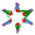
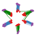
L2 Penalty=0			$h=0.01$
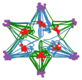
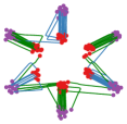
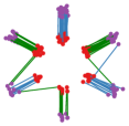
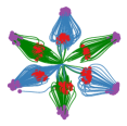
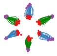
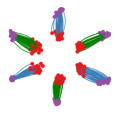
L2 Penalty$=0.01$			$h=1$

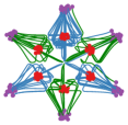
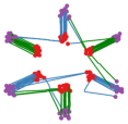
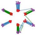
Figure 7: Rectified flows fitted with neural networks trained with different L2 penalty (left), and kernel estimator with different bandwidth $h$ (right). ${\pi}_{0}$: red dots; ${\pi}_{1}$: purple dots.

In Figure 3 of Section 2.2, the straightness is calculated as the empirical estimation of (3) based on the simulated trajectories. The relative transport cost is calculated based on $\{z_{0}^{(i)},z_{1}^{(i)}\}_{i=1}^{n}$ drawn from $(Z_{0},Z_{1})$ by simulating the flow, as $\frac{1}{n}\sum_{i=1}^{n}\left\lVert z_{1}^{(i)}-z_{0}^{(i)}\right\rVert^{2}-\left\lVert z_{1}^{(i^{*})}-z_{0}^{(i)}\right\rVert^{2}$, where $z_{1}^{(i^{*})}$ is the optimal L2 assignment of $z_{0}^{(i)}$ obtained by solving the discrete L2 optimal transport problem between $\{z_{0}^{(i)}\}$ and $\{z_{1}^{(i)}\}$. We should note that this metric is only useful in low dimensions, as it tends to be identically zero in high dimensional cases even $v^{X}$ is set to be a random neural network. This misleading phenomenon is what causes [30] to make the false hypothesis that DDIM yields L2 optimal transport.

5.2 Unconditioned Image Generation

We test rectified flow for unconditioned image generation on CIAFR-10 and a number of high resolution datasets. The methods are evaluated by the quality of generated images by Fréchet inception distance (FID) and inception score (IS), and the diversity of the generated images by the recall score following [38].

Experiment settings

For the purpose of generative modeling, we set ${\pi}_{0}$ to be the standard Gaussian distribution and ${\pi}_{1}$ the data distribution. Our implementation of rectified flow is modified upon the open-source code of  [73]. We adopt the U-Net architecture of DDPM++ [73] for representing the drift $v^{X}$, and report in Table 1 (a) and Figure 8 the results of our method and the (sub)-VP ODE from [73] using the same architecture. Other recent results using different network architectures are shown in Table 1 (b) for reference. More detailed settings can be found in the Appendix.

Method NFE($\downarrow$) IS ($\uparrow$) FID ($\downarrow$) Recall ($\uparrow$) ODE One-Step Generation (Euler solver, N=1) 1-Rectified Flow (+Distill) 1 1.13 (9.08) 378 (6.18) 0.0 (0.45) 2-Rectified Flow (+Distill) 1 8.08 (9.01) 12.21 (4.85) 0.34 (0.50) 3-Rectified Flow (+Distill) 1 8.47 (8.79) 8.15 (5.21) 0.41 (0.51) VP ODE [73] (+Distill) 1 1.20 (8.73) 451 (16.23) 0.0 (0.29) sub-VP ODE [73] (+Distill) 1 1.21 (8.80) 451 (14.32) 0.0 (0.35) ODE Full Simulation (Runge–Kutta (RK45), Adaptive $N$) 1-Rectified Flow 127 9.60 2.58 0.57 2-Rectified Flow 110 9.24 3.36 0.54 3-Rectified Flow 104 9.01 3.96 0.53 VP ODE [73] 140 9.37 3.93 0.51 sub-VP ODE [73] 146 9.46 3.16 0.55 SDE Full Simulation (Euler solver, N=2000) VP SDE [73] 2000 9.58 2.55 0.58 sub-VP SDE [73] 2000 9.56 2.61 0.58

Method NFE($\downarrow$) IS ($\uparrow$) FID ($\downarrow$) Recall ($\uparrow$) GAN One-Step Generation SNGAN [52] 1 8.22 21.7 0.44 StyleGAN2 [28] 1 9.18 8.32 0.41 StyleGAN-XL [66] 1 - 1.85 0.47 StyleGAN2 + ADA [28] 1 9.40 2.92 0.49 StyleGAN2 + DiffAug [98] 1 9.40 5.79 0.42 TransGAN + DiffAug [26] 1 9.02 9.26 0.41 GAN with U-Net One-step Generation TDPM (T=1) [99] 1 8.65 8.91 0.46 Denoising Diffusion GAN (T=1) [91] 1 8.93 14.6 0.19 ODE One Step Generation (Euler solver, N=1) DDIM Distillation [47] 1 8.36 9.36 0.51 NCSN++ (VE ODE) [73] (+Distill) 1 1.18 (2.57) 461 (254) 0.0 (0.0) ODE Full Simulation (Runge–Kutta (RK45), Adaptive $N$) NCSN++ (VE ODE) [73] 176 9.35 5.38 0.56 SDE Full Simulation (Euler solver) DDPM [23] 1000 9.46 3.21 0.57 NCSN++ (VE SDE) [73] 2000 9.83 2.38 0.59

(a) Results using the DDPM++ architecture.

(b) Recent results with different architectures reported in literature.

Table 1: Results on CIFAR10 unconditioned image generation. Fréchet Inception Distance (FID) and Inception Score (IS) measure the quality of the generated images, and recall score [38] measures diversity. The number of function evaluation (NFE) denotes the number of times we need to call the main neural network during inference. It coincides with the number of discretization steps $N$ for ODE and SDE models.

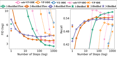
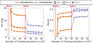
(a) FID and Recall vs. Number of Euler discretization steps $N$	(b) FID and Recall vs. Training Iterations

Figure 8: (a) Results of rectified flows and (sub-)VP ODE on CIFAR10 with different number $N$ of Euler discretization steps. (b) The FID and recall during different reflow and training steps. In (a), $k$-Distilled refers to the one-step model distilled from $k$-Rectified Flow for $k=1,2,3$.

Results

$\bullet$ Results of fully solved ODEs. As shown in Table 1 (a), the 1-rectified flow trained on the DDPM++ architecture, solved with RK45, yields the lowest FID ($2.58$) and highest recall ($0.57$) among all the ODE-based methods. In particular, the recall of 0.57 yields a substantial improvement over existing ODE and GAN methods. Using the same RK45 ODE solver, rectified flows require fewer steps to generate the images compared with VE, VP, sub-VP ODEs. The results are comparable to the fully simulated (sub-)VP SDE, which yields simulation cost.

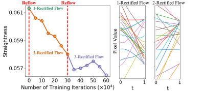
Figure 9: The straightening effect on CIFAR10. Left: the straightness measure on different reflow steps and training iterations. Right: trajectories of randomly sampled pixels following 1- and 2-rectified flow.

$\bullet$ Results on few and single step generation. As shown in Figure 8, the reflow procedure substantially improves both FID and recall in the small step regime (e.g., $N{\scriptsize\lessapprox}80$), even though it worsens the results in the large step regime due to the accumulation of error on estimating $v^{x}$. Figure 8 (b) show that each reflow leads to a noticeable improvement in FID and recall. For one-step generation $(N=1)$, the results are further boosted by distillation (see the stars in Figure 8 (a)). Overall, the distilled $k$-Rectified Flow with $k=1,2,3$ yield one-step generative models beating all previous ODEs with distillation; they also beat the reported results of one-step models with similar U-net type architectures trained using GANs (see the GAN with U-Net in Table 1 (b)).

In particular, the distilled 2-rectified flow achieves an FID of $4.85$, beating the best known one-step generative model with U-net architecture, $8.91$ (TDPM, Table 1 (b)). The recalls of both 2-rectified flow ($0.50$) and 3-rectified flow ($0.51$) outperform the best known results of GANs ($0.49$ from StyleGAN2+ADA) showing an advantage in diversity. We should note that the reported results of GANs have been carefully optimized with special techniques such as adaptive discriminator augmentation (ADA) [28], while our results are based on the vanilla implementation of rectified flow. It is likely to further improve rectified flow with proper data augmentation techniques, or the combination of GANs such as those proposed by TDPM [99] and denoising diffusion GAN [91].

$\bullet$ Reflow straightens the flow. Figure 9 shows the reflow procedure decreases improves the straightness of the flow on CIFAR10. In Figure 10 visualizes the trajectories of 1-rectified flow and 2-rectified flow on the AFHQ cat dataset: at each point $z_{t}$, we extrapolate the terminal value at $t=1$ by $\hat{z}_{1}^{t}=z_{t}+(1-t)v(z_{t},t)$; if the trajectory of ODE follows a straight line, $\hat{z}_{1}^{t}$ should not change as we vary $t$ when following the same path. We observe that $\hat{z}_{1}^{t}$ is almost independent with $t$ for 2-rectified flow, showing the path is almost straight. Moreover, even though 1-rectified flow is not straight with $\hat{z}_{1}^{t}$ over time, it still yields recognizable and clear images very early ($t\approx 0.1$). In comparison, it is need $t\approx 0.6$ to get a clear image from the extrapolation of sub-VP ODE.

High-resolution image generation

Figure 11 shows the result of 1-rectified flow on image generation on high-resolution ($256\times 256$) datasets, including LSUN Bedroom [93], LSUN Church [93], CelebA HQ [27] to AFHQ Cat [9]. We can see that it can generate high quality results across the different datasets. Figure 1 & 10 show that 1-(2-)rectified flow yields good results within one or few Euler steps.

Figure 12 shows a simple example of image editing using 1-rectified flow: We first obtain an unnatural image $z_{1}$ by stitching the upper and lower parts of two natural images, and then run 1-rectified flow backwards to get a latent code $z_{0}$. We then modify $z_{0}$ to increase its likelihood under ${\pi}_{0}$ (which is $\mathcal{N}(0,I)$) to get more naturally looking variants of the stitched image.

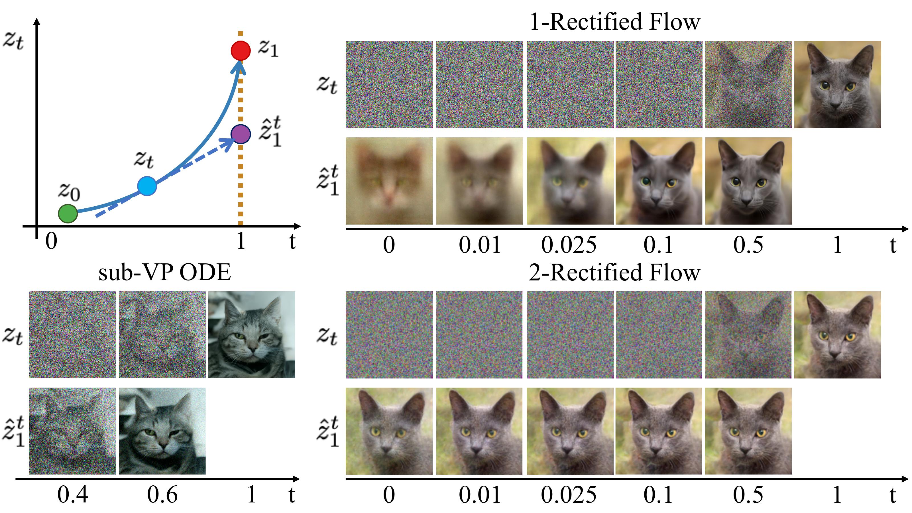
Figure 10: Sample trajectories $z_{t}$ of different flows on the AFHQ Cat dataset, and the extrapolation $\hat{z}_{1}^{t}=z_{t}+(1-t)v(z_{t},t)$ from different $z_{t}$. The same random seed is adopted for all three methods. The $\hat{z}_{1}^{t}$ of 2-rectified flow is almost independent with $t$, indicating that its trajectory is almost straight.

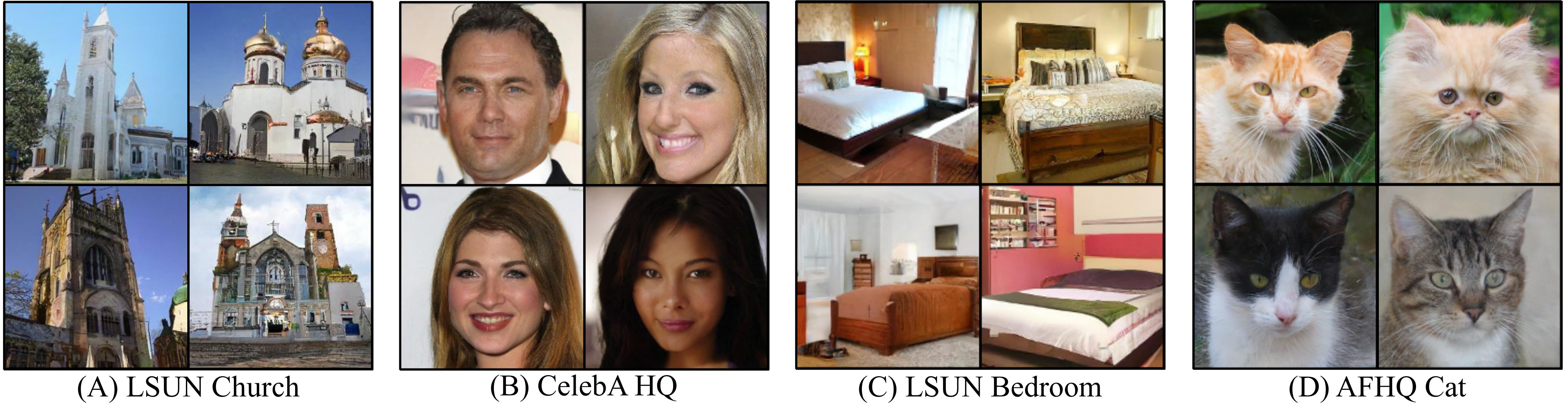
Figure 11: Examples of $256\times 256$ images generated by 1-rectified flow.

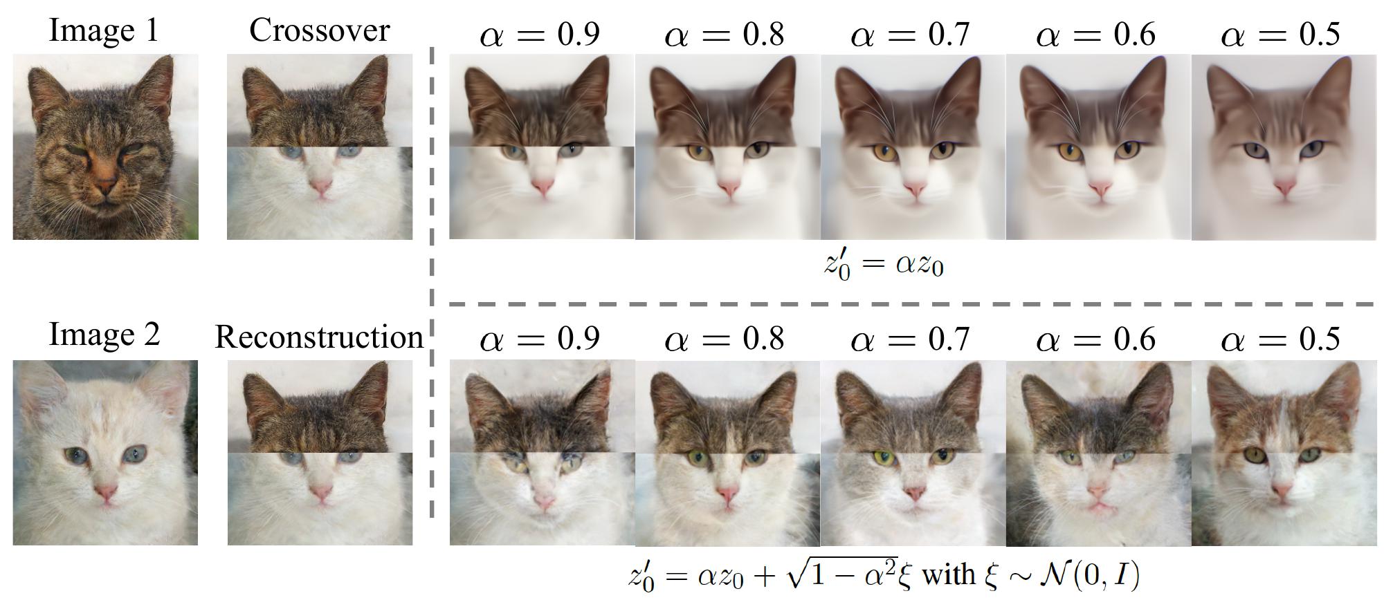
Figure 12: An example of image editing using 1-rectified flow. Here, we stitch the images of a white cat and a black cat into an unnatural image (denoted as $z_{1}$). We simulate the ODE reversely from $z_{1}$ to get the latent code $z_{0}$. Because $z_{1}$ is not a natural image, $z_{0}$ should have low likelihood under ${\pi}_{0}=\mathcal{N}(0,I)$. Hence, we move $z_{0}$ towards the high probability region of ${\pi}_{0}$ to get $z_{0}^{\prime}$ and solve the ODE forwardly to get a more realistically looking image $z_{1}^{\prime}$. The modification can be done deterministically by improving the ${\pi}_{0}$-likelihood via $z_{0}^{\prime}=\alpha z_{0}$ with $\alpha\in(0,1)$, or stochastically by Langevin dynamics, which yields a formula of $z^{\prime}_{0}=\alpha z_{0}+\sqrt{1-\alpha^{2}}\xi$ with $\xi\sim\mathcal{N}(0,I)$.

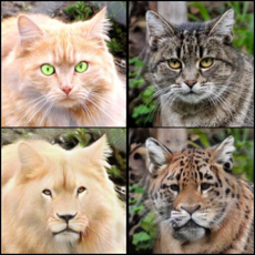
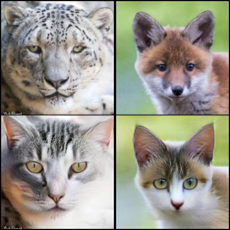
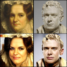
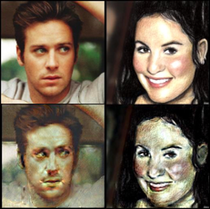
(A) Cat $\rightarrow$ Wild Animals	(B) Wild Animals $\rightarrow$ Cat	(C) MetFace $\rightarrow$ CelebA Face	(D) CelebA Face $\rightarrow$ MetFace

Figure 13: Samples of 1-rectified flow simulated with $N=100$ Euler steps between different domains.

Initialization	1-Rectified Flow	2-Rectified Flow	1-Rectified Flow	2-Rectified Flow
	$N=100$	$N=100$	$N=1$	$N=1$

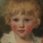
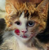
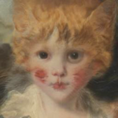
Figure 14: Samples of results of 1- and 2-rectified flow simulated with $N=1$ and $N=100$ Euler steps.

5.3 Image-to-Image Translation

Assume we are given two sets of images of different styles (a.k.a. domains), whose distributions are denoted by ${\pi}_{0},{\pi}_{1}$, respectively. We are interested in transferring the style (or other key characteristics) of the images in one domain to the other domain, in the absence of paired examples. A classical approach to achieving this is cycle-consistent adversarial networks (a.k.a. CycleGAN) [100, 25], which jointly learns a forward and backward mapping $F,G$ by minimizing the sum of adversarial losses on the two domains, regularized by a cycle consistency loss to enforce $F(G(x))\approx x$ for all image $x$.

By constructing the rectified flow of ${\pi}_{0}$ and ${\pi}_{1}$, we obtain a simple approach to image translation that requires no adversarial optimization and cycle-consistency regularization: training the rectified flow requires a simple optimization procedure and the cycle consistency is automatically in flow models satisfied due to reversibility of ODEs.

As the main goal here is to obtain good visual results, we are not interested in faithfully transferring $X_{0}\sim{\pi}_{0}$ to an $X_{1}$ that exactly follows ${\pi}_{1}$. Rather, we are interested in transferring the image styles while preserving the identity of the main object in the image. For example, when transferring a human face image to a cat face, we are interested in getting a unrealistic face of human-cat hybrid that still “looks like” the original human face.

To achieve this, let $h(x)$ be a feature mapping of image $x$ representing the styles that we are interested in transferring. Let $X_{t}=tX_{1}+(1-t)X_{0}$. Then $H_{t}=h(X_{t})$ follows an ODE of $\mathrm{d}H_{t}=\nabla h(X_{t})^{\top}(X_{1}-X_{0})\mathrm{d}t.$ Hence, to ensure that the style is transferred correctly, we propose to learn $v$ such that $H_{t}^{\prime}=h(Z_{t})$ with $\mathrm{d}Z_{t}=v(Z_{t},t)\mathrm{d}t$ approximates $H_{t}$ as much as possible. Because $\mathrm{d}H_{t}^{\prime}=\nabla h(Z_{t})^{\top}v(Z_{t},t)\mathrm{d}t$, we propose to minimize the following loss:

$$\min_{v}\int_{0}^{1}\mathbb{E}\left[\left\lVert\nabla h(X_{t})^{\top}(X_{1}-X_{0}-v(X_{t},t))\right\rVert_{2}^{2}\right]\mathrm{d}t, X_{t}=tX_{1}+(1-t)X_{0}.$$ (20)

In practice, we set $h(x)$ to be latent representation of a classifier trained to distinguish the images from the two domains ${\pi}_{0},{\pi}_{1}$, fine-tuned from a pre-trained ImageNet [77] model. Intuitively, $\nabla_{x}h(x)$ serves as a saliency score and re-weights coordinates so that the loss in (20) focuses on penalizing the error that causes significant changes on $h$.

	1-Rectified Flow
	2-Rectified Flow
	1-Rectified Flow
	2-Rectified Flow
(a) 1-rectified flow between different domains	(b) 1- and 2-rectified flow for MetFace $\rightarrow$ Cat.

Figure 15: (a) Samples of trajectories $z_{t}$ of 1- and 2-rectified flow for transferring between different domains.

Experiment settings

We set the domains ${\pi}_{0},{\pi}_{1}$ to be pairs of the AFHQ [9], MetFace [28] and CelebA-HQ [27] dataset. For each dataset, we randomly select $80\%$ as the training data and regard the rest as the test data; and the results are shown by initializing the trained flows from the test data. We resize the image to $512\times 512$. The training and network configurations generally follow the experiment settings in Section 5.2. See the appendix for detailed descriptions.

Results

Figure 1, 13, 14, 15 show examples of results of 1- and 2-rectified flow simulated with Euler method with different number of steps $N$. We can see that rectified flows can successfully transfer the styles and generate high quality images. For example, when transferring cats to wild animals, we can generate diverse images with different animal faces, e.g., fox, lion, tiger and cheetah. Moreover, with one step of reflow, 2-rectified flow returns good results with a single Euler step ($N=1$). See more examples in Appendix.

5.4 Domain Adaptation

A key challenge of applying machine learning to real-world problems is the domain shift between the training and test datasets: the performance of machine learning models may degrade significantly when tested on a novel domain different from the training set. Rectified flow can be applied to transfer the novel domain (${\pi}_{0}$) to the training domain (${\pi}_{1}$) to mitigate the impact of domain shift.

Experiment settings

We test the rectified flow for domain adaptation on a number of datasets. DomainNet [58] is a dataset of common objects in six different domain taken from DomainBed [20]. All domains from DomainNet include 345 categories (classes) of objects such as Bracelet, plane, bird and cello. Office-Home [83] is a benchmark dataset for domain adaptation which contains 4 domains where each domain consists of 65 categories. To apply our method, first we map both the training and testing data to the latent representation from final hidden layer of the pre-trained model, and construct the rectified flow on the latent representation. We use the same DDPM++ model architecture for training. For inference, we set the number of steps of our flow model as $100$ using uniform discretization. The methods are evaluated by the prediction accuracy of the transferred testing data on the classification model trained on the training data.

Results

As demonstrated in Table 2, the 1-rectified flow shows state-of-the-art performance on both DomainNet and OfficeHome. It is better or on par with the previous best approach (Deep CORAL [76]), while sustainably improve over all other methods.

Method	ERM	IRM	ARM	Mixup	MLDG	CORAL	Ours
OfficeHome	$66.5\pm 0.3$	$64.3\pm 2.2$	$64.8\pm 0.3$	$68.1\pm 0.3$	$66.8\pm 0.6$	$68.7\pm 0.3$	$\bf 69.2\pm 0.5$
DomainNet	$40.9\pm 0.1$	$33.9\pm 2.8$	$35.5\pm 0.2$	$39.2\pm 0.1$	$41.2\pm 0.1$	$\bf 41.5\pm 0.2$	$\bf 41.4\pm 0.1$

Table 2: The accuracy of the transferred testing data using different methods, on the OfficeHome and DomainNet dataset. Higher accuracy means the better performance.

Algorithm 2 Train(Data)

# Input: Data={x0, x1}
# Output: Model $v(x,t)$ for the rectified flow
initialize Model
for x0, x1 in Data: # x0, x1: samples from ${\pi}_{0}$, ${\pi}_{1}$
    Optimizer.zero_grad()
    t = torch.rand(batchsize)  # Randomly sample $t\in$ [0,1]
    Loss = ( Model(t*x1+(1-t)*x0, t) - (x1-x0) ).pow(2).mean()
    Loss.backward()
    Optimizer.step()
return Model

Algorithm 3 Sample(Model, Data)

# Input: Model $v(x,t)$ of the rectified flow
# Output: draws of the rectified coupling $(Z_{0},Z_{1})$
coupling = []
for x0, _ in Data: # x0: samples from ${\pi}_{0}$ (batchsize$\times$dim)
    x1 = model.ODE_solver(x0)
    coupling.append((x0, x1))
return coupling

Algorithm 4 Reflow(Data)

# Input: Data={x0, x1}
# Output: draws of the $K$-th rectified coupling
Coupling = Data
for $k=1,\ldots,K$:
    Model = Train(Coupling)
    Coupling = sample(Model, Data)
return Coupling

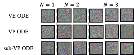
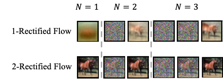
Figure 16: Few-step generation with different ODEs. Compared with VE,VP,sub-VP ODE, 1-rectified flow can generate blurry images using only 1,2,3 steps. After one time of rectification, 2-rectified flow can generate clear images with 1,2,3 steps.

Appendix A Additional Experiment Details

Experiment Configuration on CIFAR10

We conduct unconditional image generation with the CIFAR-10 dataset [36]. The resolution of the images are set to $32\times 32$. For rectified flow, we adopt the same network structure as DDPM++ in [73]. The training of the network is smoothed by exponential moving average as in [73], with a ratio of $0.999999$. We adopt Adam [31] optimizer with a learning rate of $2e-4$ and a dropout rate of $0.15$.

For reflow, we first generate 4 million pairs of $(z_{0},z_{1})$ to get a new dataset $D$, then fine-tune the $i$-rectified flow model for $300,000$ steps to get the $(i+1)$-rectified flow model. We further distill these rectified flow models for few-step generation. To get a $k$-step image generator from the $i$-rectified flow, we randomly sample $t\in\{0,1/k,\cdots,(k-1)/k\}$ during fine-tuning, instead of randomly sampling $t\in[0,1]$. Specifically, for $k=1$, we replace the L2 loss function with the LPIPS similarity [96] since it empirically brings better performance.

Expreiment Configuration on Image-to-Image Translation

In this experiment, we also adopt the same U-Net structure of DDPM++ [73] for representing the drift $v^{X}$. We follow the procedure in Algorithm 1. For the purpose of generative modeling, we set ${\pi}_{0}$ to be one domain dataset and ${\pi}_{1}$ the other domain dataset. For optimization, we use AdamW [45] optimizer with $\beta$ $(0.9,0.999)$, weight decay $0.1$ and dropout rate $0.1$. We train the model with a batch size of $4$ for $1,000$ epochs. We further apply exponential moving average (EMA) optimizer with coefficient $0.9999$. We perform grid-search on the learning rate from $\{5\times 10^{-4},2\times 10^{-4},5\times 10^{-5},2\times 10^{-5},5\times 10^{-6}\}$ and pick the model with the lowest training loss.

We use the AFHQ [9], MetFace [28] and CelebA-HQ [27] dataset. Animal Faces HQ (AFHQ) is an animal-face dataset consisting of 15,000 high-quality images at $512\times 512$ resolution. The dataset includes three domains of cat, dog, and wild animals, each providing 5000 images. MetFace consists of 1,336 high-quality PNG human-face images at $1024\times 1024$ resolution, extracted from works of art. CelebA-HQ is a human-face dataset which consists of 30,000 images at $1024\times 1024$ resolution. We randomly select $80\%$ as the training data and regard the rest as the test data, and resize the image to $512\times 512$.

Experiment Configuration on Domain Adaptation

For training the model, we apply AdamW [45] optimizer with batch size $16$, number of iterations $50$k, learning rate $10^{-4}$, weight decay $0.1$ and OneCycle [69] learning rate schedule.

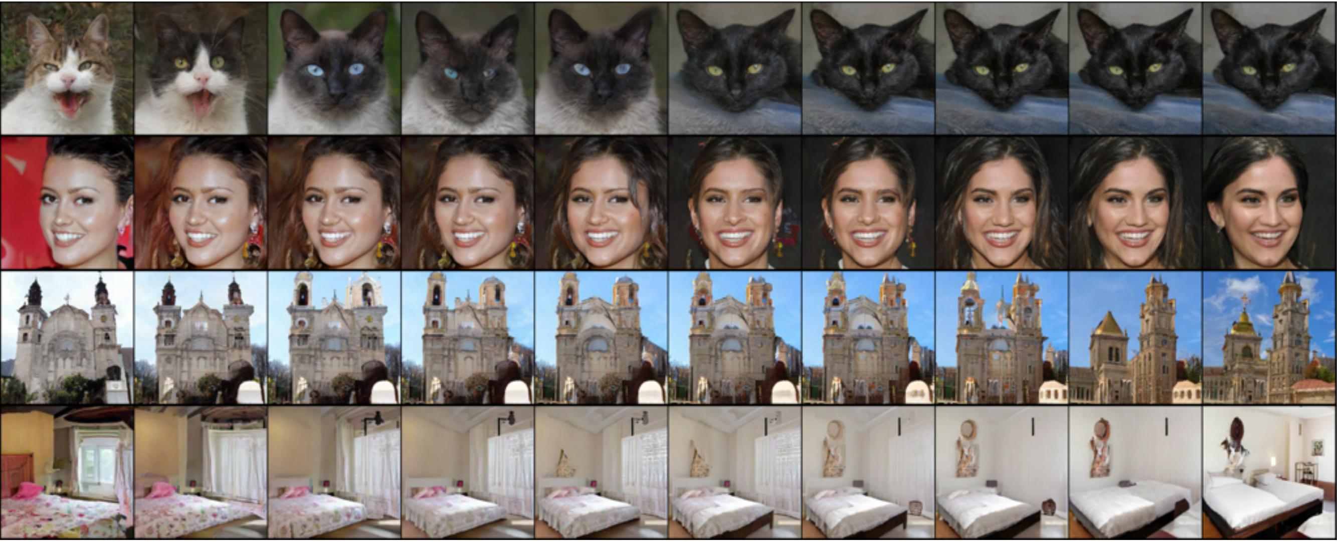
Figure 17: To visualize the latent space, we randomly sample $z_{0}$ and $z_{1}$ from $\mathcal{N}(0,I)$, and show the generated images of $\sqrt{\alpha}z_{0}+\sqrt{1-\alpha}z_{1}$ for $\alpha\in[0,1]$.

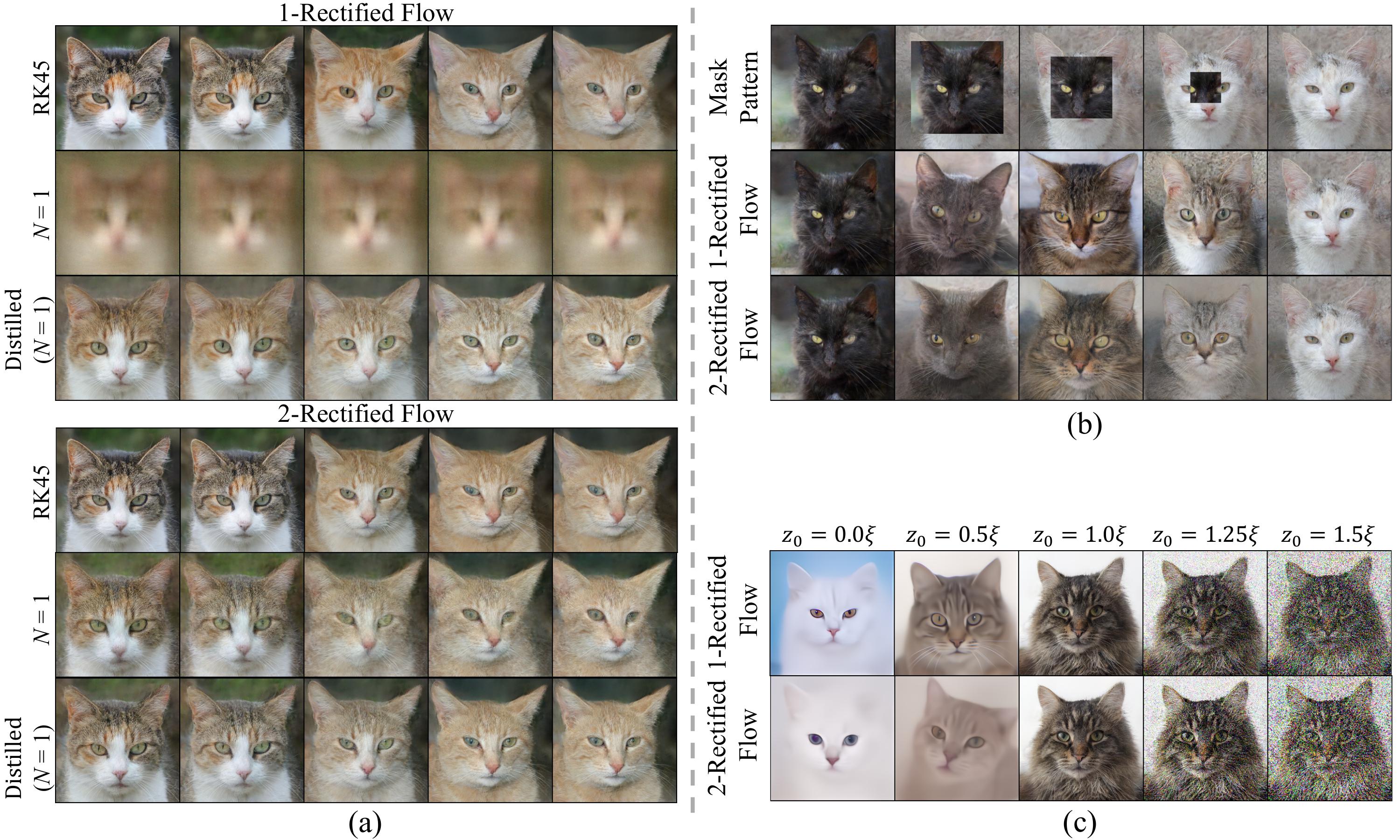
Figure 18: (a) We compare the latent space between Rectified Flow (0) and (1) using different sampling strategies with the same random seeds. We observe that (i) both 1-Rectified Flow and 2-Rectified Flow can provide a smooth latent interpolation, and their latent spaces look similar; (ii) when using one-step sampling ($N=1$), 2-Rectified Flow can still provide visually recognizable interpolation, while 1-Rectified Flow cannot; (iii) Distilled one-step models can also continuously interpolate between the images, and their latent spaces have little difference with the original flow. (b) We composite the latent codes of two images by replacing the boundary of a black cat with a white cat, then visualize the variation along the trajectory. The black cat turns into a grey cat at first, then a cat with mixing colors, and finally a white cat. (c) We randomly sample $\xi\sim\mathcal{N}(0,I)$, then generate images with $\alpha\xi$ to examine the influence of $\alpha$ on the generated images. We find $\alpha<1$ results in overly smooth images, while $\alpha>1$ leads to noisy images.

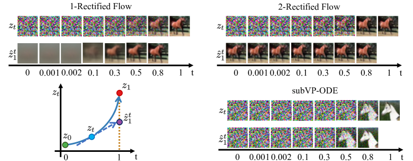
Figure 19: Sample trajectories $z_{t}$ of different flows on the CIFAR10 dataset, and the extrapolation $\hat{z}_{1}^{t}=z_{t}+(1-t)v(z_{t},t)$ from different $z_{t}$. The same random seed is adopted for all three methods. The $\hat{z}_{1}^{t}$ of 2-rectified flow is almost independent with $t$, indicating that its trajectory is almost straight.

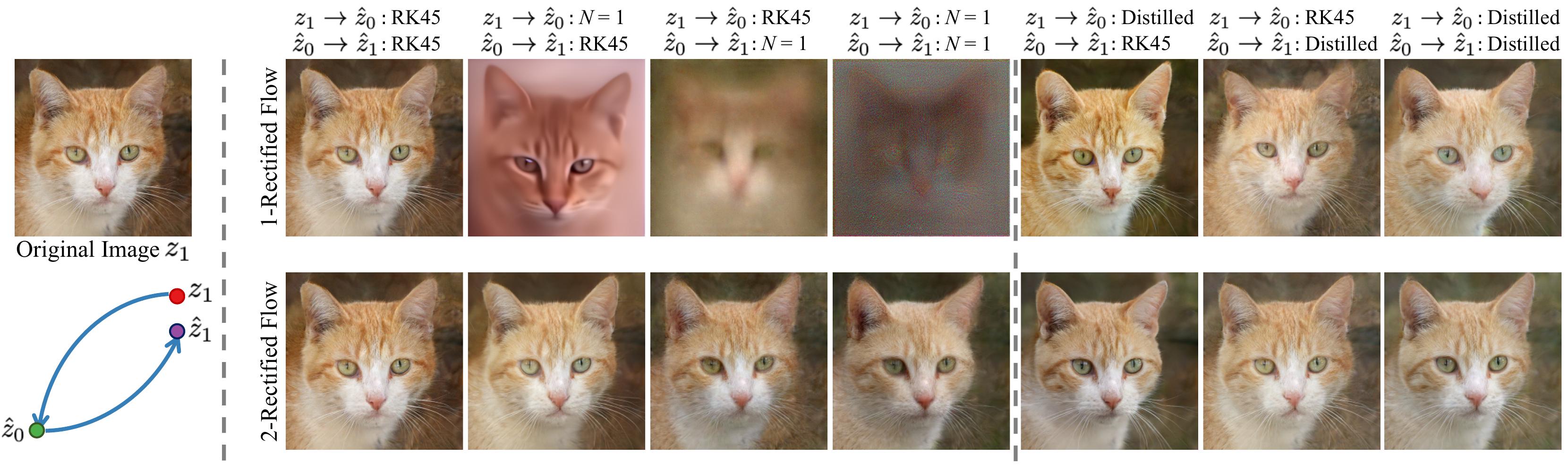
Figure 20: We perform latent space embedding / image reconstruction here. Given an image $z_{1}$, we use an reverse ODE solver to get a latent code $\hat{z}_{0}$, then use a forward ODE solver to get a reconstruction $\hat{z}_{1}$ of the image. The columns in the figure are reverse ODE solver (forward ODE solver). (i) Thanks to the‘straightening’ effect, 2-rectified flow can get meaningful latent code with only one reverse step. It can also generate recognizable images using one forward step. (ii) With the help of distilled models, one-step embedding and reconstruction is significantly improved.

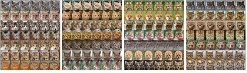
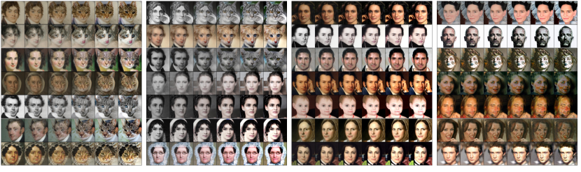
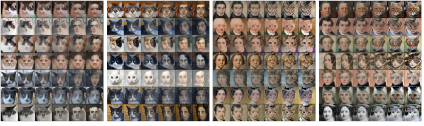
Figure 21: More results for image-to-image translation between different domains. The images in each row are time-uniformly sampled from the trajectory of 1-rectified flow solved $N=100$ Euler steps with constant step size.

References

- Ambrosio and Crippa [2008] Luigi Ambrosio and Gianluca Crippa. Existence, uniqueness, stability and differentiability properties of the flow associated to weakly differentiable vector fields. In Transport equations and multi-D hyperbolic conservation laws, pages 3–57. Springer, 2008.
- Ambrosio et al. [2021] Luigi Ambrosio, Elia Brué, and Daniele Semola. Lectures on optimal transport. Springer, 2021.
- Anderson [1982] Brian DO Anderson. Reverse-time diffusion equation models. Stochastic Processes and their Applications, 12(3):313–326, 1982.
- Arjovsky et al. [2017] Martin Arjovsky, Soumith Chintala, and Léon Bottou. Wasserstein generative adversarial networks. In International conference on machine learning, pages 214–223. PMLR, 2017.
- Bao et al. [2022] Fan Bao, Chongxuan Li, Jun Zhu, and Bo Zhang. Analytic-DPM: an analytic estimate of the optimal reverse variance in diffusion probabilistic models. arXiv preprint arXiv:2201.06503, 2022.
- Chen et al. [2018] Ricky TQ Chen, Yulia Rubanova, Jesse Bettencourt, and David K Duvenaud. Neural ordinary differential equations. Advances in neural information processing systems, 31, 2018.
- Chen et al. [2021] Tianrong Chen, Guan-Horng Liu, and Evangelos A Theodorou. Likelihood training of Schrödinger bridge using forward-backward sdes theory. arXiv preprint arXiv:2110.11291, 2021.
- Choi et al. [2021] Jooyoung Choi, Sungwon Kim, Yonghyun Jeong, Youngjune Gwon, and Sungroh Yoon. Ilvr: Conditioning method for denoising diffusion probabilistic models. arXiv preprint arXiv:2108.02938, 2021.
- Choi et al. [2020] Yunjey Choi, Youngjung Uh, Jaejun Yoo, and Jung-Woo Ha. StarGAN v2: Diverse image synthesis for multiple domains. In Proceedings of the IEEE/CVF conference on computer vision and pattern recognition, pages 8188–8197, 2020.
- Daniels et al. [2021] Max Daniels, Tyler Maunu, and Paul Hand. Score-based generative neural networks for large-scale optimal transport. Advances in neural information processing systems, 34:12955–12965, 2021.
- De Bortoli et al. [2021] Valentin De Bortoli, James Thornton, Jeremy Heng, and Arnaud Doucet. Diffusion Schrödinger bridge with applications to score-based generative modeling. Advances in Neural Information Processing Systems, 34, 2021.
- Dhariwal and Nichol [2021] Prafulla Dhariwal and Alexander Nichol. Diffusion models beat GANs on image synthesis. Advances in Neural Information Processing Systems, 34, 2021.
- Dinh et al. [2014] Laurent Dinh, David Krueger, and Yoshua Bengio. Nice: Non-linear independent components estimation. arXiv preprint arXiv:1410.8516, 2014.
- Dinh et al. [2016] Laurent Dinh, Jascha Sohl-Dickstein, and Samy Bengio. Density estimation using real nvp. arXiv preprint arXiv:1605.08803, 2016.
- Figalli and Glaudo [2021] Alessio Figalli and Federico Glaudo. An Invitation to Optimal Transport, Wasserstein Distances, and Gradient Flows. 2021.
- Flamary et al. [2016] R Flamary, N Courty, D Tuia, and A Rakotomamonjy. Optimal transport for domain adaptation. IEEE Trans. Pattern Anal. Mach. Intell, 1, 2016.
- Föllmer [1985] Hans Föllmer. An entropy approach to the time reversal of diffusion processes. In Stochastic Differential Systems Filtering and Control, pages 156–163. Springer, 1985.
- Franzese et al. [2022] Giulio Franzese, Simone Rossi, Lixuan Yang, Alessandro Finamore, Dario Rossi, Maurizio Filippone, and Pietro Michiardi. How much is enough? a study on diffusion times in score-based generative models. arXiv preprint arXiv:2206.05173, 2022.
- Goodfellow et al. [2014] Ian Goodfellow, Jean Pouget-Abadie, Mehdi Mirza, Bing Xu, David Warde-Farley, Sherjil Ozair, Aaron Courville, and Yoshua Bengio. Generative adversarial nets. Advances in neural information processing systems, 27, 2014.
- Gulrajani and Lopez-Paz [2020] Ishaan Gulrajani and David Lopez-Paz. In search of lost domain generalization. arXiv preprint arXiv:2007.01434, 2020.
- Harvey et al. [2022] William Harvey, Saeid Naderiparizi, Vaden Masrani, Christian Weilbach, and Frank Wood. Flexible diffusion modeling of long videos. arXiv preprint arXiv:2205.11495, 2022.
- Haussmann and Pardoux [1986] Ulrich G Haussmann and Etienne Pardoux. Time reversal of diffusions. The Annals of Probability, pages 1188–1205, 1986.
- Ho et al. [2020] Jonathan Ho, Ajay Jain, and Pieter Abbeel. Denoising diffusion probabilistic models. Advances in Neural Information Processing Systems, 33:6840–6851, 2020.
- Ho et al. [2022] Jonathan Ho, Tim Salimans, Alexey Gritsenko, William Chan, Mohammad Norouzi, and David J Fleet. Video diffusion models. arXiv preprint arXiv:2204.03458, 2022.
- Isola et al. [2017] Phillip Isola, Jun-Yan Zhu, Tinghui Zhou, and Alexei A Efros. Image-to-image translation with conditional adversarial networks. In Proceedings of the IEEE conference on computer vision and pattern recognition, pages 1125–1134, 2017.
- Jiang et al. [2021] Yifan Jiang, Shiyu Chang, and Zhangyang Wang. TransGAN: Two pure transformers can make one strong GAN, and that can scale up. Advances in Neural Information Processing Systems, 34, 2021.
- Karras et al. [2018] Tero Karras, Timo Aila, Samuli Laine, and Jaakko Lehtinen. Progressive growing of GANs for improved quality, stability, and variation. In International Conference on Learning Representations, 2018.
- Karras et al. [2020] Tero Karras, Miika Aittala, Janne Hellsten, Samuli Laine, Jaakko Lehtinen, and Timo Aila. Training generative adversarial networks with limited data. Advances in Neural Information Processing Systems, 33:12104–12114, 2020.
- Karras et al. [2022] Tero Karras, Miika Aittala, Timo Aila, and Samuli Laine. Elucidating the design space of diffusion-based generative models. arXiv preprint arXiv:2206.00364, 2022.
- Khrulkov and Oseledets [2022] Valentin Khrulkov and Ivan Oseledets. Understanding DDPM latent codes through optimal transport. arXiv preprint arXiv:2202.07477, 2022.
- Kingma and Ba [2014] Diederik P Kingma and Jimmy Ba. Adam: A method for stochastic optimization. arXiv preprint arXiv:1412.6980, 2014.
- Kingma and Welling [2013] Diederik P Kingma and Max Welling. Auto-encoding variational bayes. arXiv preprint arXiv:1312.6114, 2013.
- Kong et al. [2020] Zhifeng Kong, Wei Ping, Jiaji Huang, Kexin Zhao, and Bryan Catanzaro. Diffwave: A versatile diffusion model for audio synthesis. In International Conference on Learning Representations, 2020.
- Korotin et al. [2021] Alexander Korotin, Lingxiao Li, Aude Genevay, Justin M Solomon, Alexander Filippov, and Evgeny Burnaev. Do neural optimal transport solvers work? a continuous wasserstein-2 benchmark. Advances in Neural Information Processing Systems, 34:14593–14605, 2021.
- Korotin et al. [2022] Alexander Korotin, Daniil Selikhanovych, and Evgeny Burnaev. Neural optimal transport. arXiv preprint arXiv:2201.12220, 2022.
- Krizhevsky et al. [2009] Alex Krizhevsky, Geoffrey Hinton, et al. Learning multiple layers of features from tiny images. 2009.
- Kurtz [2011] Thomas G Kurtz. Equivalence of stochastic equations and martingale problems. In Stochastic analysis 2010, pages 113–130. Springer, 2011.
- Kynkäänniemi et al. [2019] Tuomas Kynkäänniemi, Tero Karras, Samuli Laine, Jaakko Lehtinen, and Timo Aila. Improved precision and recall metric for assessing generative models. Advances in Neural Information Processing Systems, 32, 2019.
- Lavenant and Santambrogio [2022] Hugo Lavenant and Filippo Santambrogio. The flow map of the fokker–planck equation does not provide optimal transport. Applied Mathematics Letters, page 108225, 2022.
- Lee and Han [2021] Junhyeok Lee and Seungu Han. Nu-wave: A diffusion probabilistic model for neural audio upsampling. arXiv preprint arXiv:2104.02321, 2021.
- Li et al. [2022] Xiang Lisa Li, John Thickstun, Ishaan Gulrajani, Percy Liang, and Tatsunori B Hashimoto. Diffusion-lm improves controllable text generation. arXiv preprint arXiv:2205.14217, 2022.
- Liu [2022] Qiang Liu. On rectified flow and optimal coupling. preprint, 2022.
- Liu et al. [2021] Xingchao Liu, Chengyue Gong, Lemeng Wu, Shujian Zhang, Hao Su, and Qiang Liu. Fusedream: Training-free text-to-image generation with improved clip+ gan space optimization. arXiv preprint arXiv:2112.01573, 2021.
- Liu et al. [2022] Xingchao Liu, Lemeng Wu, Mao Ye, and Qiang Liu. Let us build bridges: Understanding and extending diffusion generative models. arXiv preprint arXiv:2208.14699, 2022.
- Loshchilov and Hutter [2017] Ilya Loshchilov and Frank Hutter. Decoupled weight decay regularization. arXiv preprint arXiv:1711.05101, 2017.
- Lu et al. [2022] Cheng Lu, Yuhao Zhou, Fan Bao, Jianfei Chen, Chongxuan Li, and Jun Zhu. DPM-solver: A fast ODE solver for diffusion probabilistic model sampling in around 10 steps. arXiv preprint arXiv:2206.00927, 2022.
- Luhman and Luhman [2021] Eric Luhman and Troy Luhman. Knowledge distillation in iterative generative models for improved sampling speed. arXiv preprint arXiv:2101.02388, 2021.
- Lyu et al. [2022] Zhaoyang Lyu, Xudong Xu, Ceyuan Yang, Dahua Lin, and Bo Dai. Accelerating diffusion models via early stop of the diffusion process. arXiv preprint arXiv:2205.12524, 2022.
- Makkuva et al. [2020] Ashok Makkuva, Amirhossein Taghvaei, Sewoong Oh, and Jason Lee. Optimal transport mapping via input convex neural networks. In International Conference on Machine Learning, pages 6672–6681. PMLR, 2020.
- Meng et al. [2021] Chenlin Meng, Yang Song, Jiaming Song, Jiajun Wu, Jun-Yan Zhu, and Stefano Ermon. Sdedit: Image synthesis and editing with stochastic differential equations. arXiv preprint arXiv:2108.01073, 2021.
- Mittal et al. [2021] Gautam Mittal, Jesse Engel, Curtis Hawthorne, and Ian Simon. Symbolic music generation with diffusion models. arXiv preprint arXiv:2103.16091, 2021.
- Miyato et al. [2018] Takeru Miyato, Toshiki Kataoka, Masanori Koyama, and Yuichi Yoshida. Spectral normalization for generative adversarial networks. In International Conference on Learning Representations, 2018.
- Nichol et al. [2021] Alex Nichol, Prafulla Dhariwal, Aditya Ramesh, Pranav Shyam, Pamela Mishkin, Bob McGrew, Ilya Sutskever, and Mark Chen. Glide: Towards photorealistic image generation and editing with text-guided diffusion models. arXiv preprint arXiv:2112.10741, 2021.
- Nichol and Dhariwal [2021] Alexander Quinn Nichol and Prafulla Dhariwal. Improved denoising diffusion probabilistic models. In International Conference on Machine Learning, pages 8162–8171. PMLR, 2021.
- Onken et al. [2021] Derek Onken, Samy Wu Fung, Xingjian Li, and Lars Ruthotto. Ot-flow: Fast and accurate continuous normalizing flows via optimal transport. In Proceedings of the AAAI Conference on Artificial Intelligence, volume 35, pages 9223–9232, 2021.
- Papamakarios et al. [2021] George Papamakarios, Eric T Nalisnick, Danilo Jimenez Rezende, Shakir Mohamed, and Balaji Lakshminarayanan. Normalizing flows for probabilistic modeling and inference. J. Mach. Learn. Res., 22(57):1–64, 2021.
- Peluchetti [2021] Stefano Peluchetti. Non-denoising forward-time diffusions. 2021.
- Peng et al. [2019] Xingchao Peng, Qinxun Bai, Xide Xia, Zijun Huang, Kate Saenko, and Bo Wang. Moment matching for multi-source domain adaptation. In Proceedings of the IEEE/CVF international conference on computer vision, pages 1406–1415, 2019.
- Peyré et al. [2019] Gabriel Peyré, Marco Cuturi, et al. Computational optimal transport: With applications to data science. Foundations and Trends® in Machine Learning, 11(5-6):355–607, 2019.
- Popov et al. [2021] Vadim Popov, Ivan Vovk, Vladimir Gogoryan, Tasnima Sadekova, and Mikhail Kudinov. Grad-tts: A diffusion probabilistic model for text-to-speech. In International Conference on Machine Learning, pages 8599–8608. PMLR, 2021.
- Ramesh et al. [2022] Aditya Ramesh, Prafulla Dhariwal, Alex Nichol, Casey Chu, and Mark Chen. Hierarchical text-conditional image generation with clip latents. arXiv preprint arXiv:2204.06125, 2022.
- Rezende and Mohamed [2015] Danilo Rezende and Shakir Mohamed. Variational inference with normalizing flows. In International conference on machine learning, pages 1530–1538. PMLR, 2015.
- Rout et al. [2021] Litu Rout, Alexander Korotin, and Evgeny Burnaev. Generative modeling with optimal transport maps. arXiv preprint arXiv:2110.02999, 2021.
- Saharia et al. [2022] Chitwan Saharia, William Chan, Saurabh Saxena, Lala Li, Jay Whang, Emily Denton, Seyed Kamyar Seyed Ghasemipour, Burcu Karagol Ayan, S Sara Mahdavi, Rapha Gontijo Lopes, et al. Photorealistic text-to-image diffusion models with deep language understanding. arXiv preprint arXiv:2205.11487, 2022.
- Santambrogio [2015] Filippo Santambrogio. Optimal transport for applied mathematicians. Birkäuser, NY, 55(58-63):94, 2015.
- Sauer et al. [2022] Axel Sauer, Katja Schwarz, and Andreas Geiger. StyleGAN-XL: Scaling StyleGAN to large diverse datasets. In Special Interest Group on Computer Graphics and Interactive Techniques Conference Proceedings, pages 1–10, 2022.
- Seguy et al. [2017] Vivien Seguy, Bharath Bhushan Damodaran, Rémi Flamary, Nicolas Courty, Antoine Rolet, and Mathieu Blondel. Large-scale optimal transport and mapping estimation. arXiv preprint arXiv:1711.02283, 2017.
- Sinha et al. [2021] Abhishek Sinha, Jiaming Song, Chenlin Meng, and Stefano Ermon. D2C: Diffusion-decoding models for few-shot conditional generation. Advances in Neural Information Processing Systems, 34:12533–12548, 2021.
- Smith and Topin [2019] Leslie N Smith and Nicholay Topin. Super-convergence: Very fast training of neural networks using large learning rates. In Artificial intelligence and machine learning for multi-domain operations applications, volume 11006, pages 369–386. SPIE, 2019.
- Song et al. [2020a] Jiaming Song, Chenlin Meng, and Stefano Ermon. Denoising diffusion implicit models. In International Conference on Learning Representations, 2020a.
- Song and Ermon [2019] Yang Song and Stefano Ermon. Generative modeling by estimating gradients of the data distribution. Advances in Neural Information Processing Systems, 32, 2019.
- Song and Ermon [2020] Yang Song and Stefano Ermon. Improved techniques for training score-based generative models. Advances in neural information processing systems, 33:12438–12448, 2020.
- Song et al. [2020b] Yang Song, Jascha Sohl-Dickstein, Diederik P Kingma, Abhishek Kumar, Stefano Ermon, and Ben Poole. Score-based generative modeling through stochastic differential equations. In International Conference on Learning Representations, 2020b.
- Song et al. [2021] Yang Song, Conor Durkan, Iain Murray, and Stefano Ermon. Maximum likelihood training of score-based diffusion models. Advances in Neural Information Processing Systems, 34, 2021.
- Su et al. [2022] Xuan Su, Jiaming Song, Chenlin Meng, and Stefano Ermon. Dual diffusion implicit bridges for image-to-image translation. arXiv preprint arXiv:2203.08382, 2022.
- Sun and Saenko [2016] Baochen Sun and Kate Saenko. Deep coral: Correlation alignment for deep domain adaptation. In European conference on computer vision, pages 443–450. Springer, 2016.
- Tan and Le [2019] Mingxing Tan and Quoc Le. Efficientnet: Rethinking model scaling for convolutional neural networks. In International conference on machine learning, pages 6105–6114. PMLR, 2019.
- Tanana [2021] Anastasiya Tanana. Comparison of transport map generated by heat flow interpolation and the optimal transport brenier map. Communications in Contemporary Mathematics, 23(06):2050025, 2021.
- Trigila and Tabak [2016] Giulio Trigila and Esteban G Tabak. Data-driven optimal transport. Communications on Pure and Applied Mathematics, 69(4):613–648, 2016.
- Tzen and Raginsky [2019] Belinda Tzen and Maxim Raginsky. Theoretical guarantees for sampling and inference in generative models with latent diffusions. In Conference on Learning Theory, pages 3084–3114. PMLR, 2019.
- Vahdat et al. [2021] Arash Vahdat, Karsten Kreis, and Jan Kautz. Score-based generative modeling in latent space. Advances in Neural Information Processing Systems, 34:11287–11302, 2021.
- Vargas et al. [2021] Francisco Vargas, Pierre Thodoroff, Austen Lamacraft, and Neil Lawrence. Solving Schrödinger bridges via maximum likelihood. Entropy, 23(9):1134, 2021.
- Venkateswara et al. [2017] Hemanth Venkateswara, Jose Eusebio, Shayok Chakraborty, and Sethuraman Panchanathan. Deep hashing network for unsupervised domain adaptation. In Proceedings of the IEEE conference on computer vision and pattern recognition, pages 5018–5027, 2017.
- Villani [2009] Cédric Villani. Optimal transport: old and new, volume 338. Springer, 2009.
- Villani [2021] Cédric Villani. Topics in optimal transportation, volume 58. American Mathematical Soc., 2021.
- Virtanen et al. [2020] Pauli Virtanen, Ralf Gommers, Travis E. Oliphant, Matt Haberland, Tyler Reddy, David Cournapeau, Evgeni Burovski, Pearu Peterson, Warren Weckesser, Jonathan Bright, Stéfan J. van der Walt, Matthew Brett, Joshua Wilson, K. Jarrod Millman, Nikolay Mayorov, Andrew R. J. Nelson, Eric Jones, Robert Kern, Eric Larson, C J Carey, İlhan Polat, Yu Feng, Eric W. Moore, Jake VanderPlas, Denis Laxalde, Josef Perktold, Robert Cimrman, Ian Henriksen, E. A. Quintero, Charles R. Harris, Anne M. Archibald, Antônio H. Ribeiro, Fabian Pedregosa, Paul van Mulbregt, and SciPy 1.0 Contributors. SciPy 1.0: Fundamental Algorithms for Scientific Computing in Python. Nature Methods, 17:261–272, 2020. doi: 10.1038/s41592-019-0686-2.
- Wang et al. [2021] Gefei Wang, Yuling Jiao, Qian Xu, Yang Wang, and Can Yang. Deep generative learning via Schrödinger bridge. In International Conference on Machine Learning, pages 10794–10804. PMLR, 2021.
- Wang et al. [2022] Rose E Wang, Esin Durmus, Noah Goodman, and Tatsunori Hashimoto. Language modeling via stochastic processes. arXiv preprint arXiv:2203.11370, 2022.
- Wehenkel and Louppe [2021] Antoine Wehenkel and Gilles Louppe. Diffusion priors in variational autoencoders. arXiv preprint arXiv:2106.15671, 2021.
- Wu et al. [2022] Lemeng Wu, Chengyue Gong, Xingchao Liu, Mao Ye, and Qiang Liu. Diffusion-based molecule generation with informative prior bridges. arXiv preprint, 2022.
- Xiao et al. [2021] Zhisheng Xiao, Karsten Kreis, and Arash Vahdat. Tackling the generative learning trilemma with denoising diffusion GANs. arXiv preprint arXiv:2112.07804, 2021.
- Yang et al. [2022] Ruihan Yang, Prakhar Srivastava, and Stephan Mandt. Diffusion probabilistic modeling for video generation. arXiv preprint arXiv:2203.09481, 2022.
- Yu et al. [2015] Fisher Yu, Ari Seff, Yinda Zhang, Shuran Song, Thomas Funkhouser, and Jianxiong Xiao. Lsun: Construction of a large-scale image dataset using deep learning with humans in the loop. arXiv preprint arXiv:1506.03365, 2015.
- Zhang and Chen [2022] Qinsheng Zhang and Yongxin Chen. Fast sampling of diffusion models with exponential integrator. arXiv preprint arXiv:2204.13902, 2022.
- Zhang et al. [2022] Qinsheng Zhang, Molei Tao, and Yongxin Chen. gDDIM: Generalized denoising diffusion implicit models. arXiv preprint arXiv:2206.05564, 2022.
- Zhang et al. [2018] Richard Zhang, Phillip Isola, Alexei A Efros, Eli Shechtman, and Oliver Wang. The unreasonable effectiveness of deep features as a perceptual metric. In Proceedings of the IEEE conference on computer vision and pattern recognition, pages 586–595, 2018.
- Zhao et al. [2022] Min Zhao, Fan Bao, Chongxuan Li, and Jun Zhu. EGSDE: Unpaired image-to-image translation via energy-guided stochastic differential equations. arXiv preprint arXiv:2207.06635, 2022.
- Zhao et al. [2020] Shengyu Zhao, Zhijian Liu, Ji Lin, Jun-Yan Zhu, and Song Han. Differentiable augmentation for data-efficient GAN training. Advances in Neural Information Processing Systems, 33:7559–7570, 2020.
- Zheng et al. [2022] Huangjie Zheng, Pengcheng He, Weizhu Chen, and Mingyuan Zhou. Truncated diffusion probabilistic models. arXiv preprint arXiv:2202.09671, 2022.
- Zhu et al. [2017] Jun-Yan Zhu, Taesung Park, Phillip Isola, and Alexei A Efros. Unpaired image-to-image translation using cycle-consistent adversarial networks. In Proceedings of the IEEE international conference on computer vision, pages 2223–2232, 2017.