A Computationally Efficient algorithm to estimate the Parameters of a Two-Dimensional Chirp Model with the product term

Abstract

Chirp signal models and their generalizations have been used to model many natural and man-made phenomena in signal processing and time series literature. In recent times, several methods have been proposed for parameter estimation of these models. These methods however are either statistically sub-optimal or computationally burdensome, specially for two dimensional (2D) chirp models. In this paper, we consider the problem of parameter estimation of 2D chirp models and propose a computationally efficient estimator and establish asymptotic theoretical properties of the proposed estimators. And the proposed estimators are observed to have the same rates of convergence as the least squares estimators (LSEs). Furthermore, the proposed estimators of chirp rate parameters are shown to be asymptotically optimal. Extensive and detailed numerical simulations are conducted, which support theoretical results of the proposed estimators.

 
 
Keywords: 2D Chirp model, least squares estimators, stationary linear process, consistency, asymptotic normality.

1 Introduction

This paper addresses the problem of parameter estimation of a 2D chirp signal model defined as follows:

$$y(m,n) =A^{0}\cos(\alpha^{0}m+\beta^{0}m^{2}+\gamma^{0}n+\delta^{0}n^{2}+\mu^{0}mn)$$

$$+B^{0}\sin(\alpha^{0}m+\beta^{0}m^{2}+\gamma^{0}n+\delta^{0}n^{2}+\mu^{0}mn)+X(m,n),$$ (1)

$$\hskip 15.0ptm=1,2,\ldots,M,n=1,2,\ldots,N.$$

Here, $y(m,n)$ is the observed real valued signal and $X(m,n)$ is the additive noise term. $A^{0},B^{0}$ are amplitude parameters, $\alpha^{0},\gamma^{0}$ are frequency parameters, $\beta^{0},\delta^{0}$ are frequency rates or chirp rates, and $\mu^{0}$ is the coefficient of product term. $\mathrm{\bm{\xi}}^{0}=(\alpha^{0},\beta^{0},\gamma^{0},\delta^{0},\mu^{0})^{\top}\hskip 2.0pt$ represents vector of non-linear parameters. This model can be used to describe signals having constant amplitude with frequency to be a linear function of spatial co-ordinates. The product term $mn$ in such chirp models (1), is an important characteristic of numerous measurement interferometric signals or radar signal returns.
 
The parameter estimation problem for model (1) is encountered in many real-life applications such as 2D-homomorphic signal processing, magnetic resonance imaging (MRI), optical imaging, interferometric synthetic aperture radar (INSAR), modeling non-homogeneous patterns in the texture image captured by a camera due to perspective or orientation ( see e.g., [6],[8], [9] and the references cited therein). 2D chirps have been used as a spreading function in digital watermarking which is also helpful in data security, medical safety, fingerprinting, and observing content manipulations, see [23]. 2D chirp signals have also been used to model Newton’s rings [13]. These rings are predominantly used in testing spherical and flatting optical surface and curvature radius measurement.
 
Many algorithms based on different approaches have been put forward in the literature to solve such problems. Polynomial phase differencing (PD) operator was introduced in [6] as an extension of the polynomial phase transform proposed in [20]. Several works [7], [8] and [9] utilized PD operator to develop computationally efficient algorithms for estimating similar polynomial phase signals. Cubic phase function (CPF) proposed in [19], was extended in [22] for similar 2D chirp signal modelling. Further, CPF was utilized to estimate 2D cubic phase signal using genetic algorithm in [3]. Consistency and asymptotic normality of LSEs for a general 2D polynomial phase signal (PPS) model have been derived in [16]. A finite step computationally efficient procedure for a similar 2D chirp signal model proposed in [14] was proved asymptotically equivalent to LSEs. Quasi-Maximum Likelihood (QML) algorithm [4] proposed for 1D PPS, was generalized for 2D PPS in [5]. Further approximate least squares estimators (ALSEs) proposed in [11] have been proved to be asymptotically equivalent to LSEs. An efficient estimation procedure based on fixed dimension technique, presented in [12] was shown to be equivalent to the optimal LSEs, for a 2D chirp model without the product term $mn$.
 
Estimators based on phase differencing strategies or high order ambiguity function (HAF) or some of their modifications are computationally easier to obtain. However, the performance of estimation deteriorate below a relatively high signal-to-noise ratio (SNR) threshold and are sub-optimal. Methods that use PD in the steps of estimation, usually estimate coefficients of the highest degree first, and then subsequently estimate the coefficients of a lower degree from the demodulated or de-chirped signal. Therefore, the estimation error of highest degree coefficients accumulates and affects estimation accuracy of lower degree coefficients quite seriously. For more details, one can refer to [1], [5] and [21]. Till date, there is no detailed study of the theoretical properties of the estimators such as CPF and QML, such as strong consistency and asymptotic normality. Recently, optimal estimators for a simpler 2D chirp model without the interaction term have been developed in [12]. However, the results in [12] cannot be generalized directly for the underlying model (1). It may be noted that the model considered in this paper is more general, as it takes into account the interaction term $\mu^{0}mn$. Due to the presence of this interaction term coefficient $\mu^{0}$, the estimation becomes more difficult as the estimators of $\alpha^{0}$ and $\gamma^{0}$ are no longer independent (as in the case for [12]), and hence making their computation as well as study of theoretical analysis becomes more challenging. The problem becomes more complicated under the assumption of general stationary linear process error assumption.
 
The main contributions of this paper are; providing a computationally efficient algorithm to estimate the parameters of the model defined in (1), and further establishing theoretical asymptotic properties of the proposed estimators. The proposed algorithm is motivated by the fact that a 2D chirp model with five non-linear parameters can be viewed through a number of 1D chirp models with two non-linear parameters and hence computational complexity of 2D models can be reduced.
 
The key attributes of the proposed method are that it is computationally faster than the conventional optimal methods such as LSEs, maximum likelihood estimators, or ALSEs and at the same time, having desirable statistical properties such as, attaining same rates of convergence as the optimal LSEs. In fact, the proposed estimators of the chirp rate parameters, then these have the same asymptotic variance as that of the traditional LSEs, and hence are statistically optimal.
 
The rest of the paper is organised as follows: the methodology to obtain the proposed estimators is presented in Section 2. The model assumptions and the asymptotic theoretical results are given in Section 3. In Section 4, the finite sample performance of the proposed estimators is demonstrated through simulation studies. In this section, a comparison of the performance of the proposed estimators with the state-of-the-art methods such as least squares method, approximate least squares method, and 2D multilag HAF method is also presented. Finally, Section 5 concludes the paper, followed by detailed proofs in appendices.

2 Estimation Methodology

In this section, we present the proposed method of estimation. Let the data matrix for model (1) be denoted as

$$\bm{Y}=\begin{bmatrix}y(1,1)&y(1,2)&\ldots&y(1,N)\\ y(2,1)&y(2,2)&\ldots&y(2,N)\\ \vdots&\vdots&\ddots&\vdots\\ y(M,1)&y(M,2)&\ldots&y(M,N)\end{bmatrix}_{M\times N}.$$

The proposed algorithm uses the fact that for each fixed column (or row) of $\bm{Y}$, the 2D chirp model breaks down to a cascade of 1D chirp models.
 
Realise that if we fix one dimension say $n=n_{0}$ in (1), then the 2D chirp can be seen as 1-D chirp for $m=1,2,\ldots,M$, as follows:

$$y(m,n_{0})=A^{0}(n_{0})\cos\big{(}(\alpha^{0}+n_{0}\mu^{0})m+\beta^{0}m^{2}\big{)} +B^{0}(n_{0})\sin\big{(}(\alpha^{0}+n_{0}\mu^{0})m+\beta^{0}m^{2}\big{)}$$

$$+X(m,n_{0}),$$ (2)

$$\text{where, }\hskip 10.0ptA^{0}(n_{0}) =A^{0}\cos(\gamma^{0}n_{0}+\delta^{0}n_{0}^{2})+B^{0}\sin(\gamma^{0}n_{0}+\delta^{0}n_{0}^{2}),$$

$$\hskip 45.0ptB^{0}(n_{0}) =-A^{0}\sin(\gamma^{0}n_{0}+\delta^{0}n_{0}^{2})+B^{0}\cos(\gamma^{0}n_{0}+\delta^{0}n_{0}^{2}).$$

Similarly, for a fixed $m=m_{0}$, we have 1-D chirp for $n=1,2,\ldots,N,$

$$y(m_{0},n)=\widetilde{A}^{0}(m_{0})\cos\big{(}(\gamma^{0}+m_{0}\mu^{0})n+\delta^{0}n^{2}\big{)} +\widetilde{B}^{0}(m_{0})\sin\big{(}(\gamma^{0}+m_{0}\mu^{0})n+\delta^{0}n^{2}\big{)}$$

$$+X(m_{0},n).$$ (3)

Equation (2) represents 1-D chirp signal model with $\alpha^{0}+n_{0}\mu^{0}$ and $\beta^{0}$ as the frequency and frequency rate parameters respectively. Similarly, equation (2) represents 1-D chirp signal model with $\gamma^{0}+m_{0}\mu^{0}$ and $\delta^{0}$ as the frequency and frequency rate parameters respectively.
 
Hence, our methodology is developed by estimating parameters of these 1D chirps based on a particular column (or row) vector of data matrix, rather than estimating the whole 2D chirp parameters based on the full data matrix. Therefore this procedure reduces computational burden to estimate model parameters drastically. Further suppose column vector $\bm{Y}_{Mn_{0}}$ denotes the $n_{0}^{th}$ column of data matrix $\bm{Y}$ and column vector $\bm{Y}_{m_{0}N}$ denotes the transpose of $m_{0}^{th}$ row of data matrix $\bm{Y}$. Define $Z_{k}(\alpha_{1},\alpha_{2})$ matrix as

$$Z_{k}(\alpha_{1},\alpha_{2})=\begin{bmatrix}\cos(\alpha_{1}+\alpha_{2})&\sin(\alpha_{1}+\alpha_{2})\\ \cos(\alpha_{1}2+\alpha_{2}2^{2})&\sin(\alpha_{1}2+\alpha_{2}2^{2})\\ \vdots&\vdots\\ \cos(\alpha_{1}k+\alpha_{2}k^{2})&\sin(\alpha_{1}k+\alpha_{2}k^{2})\\ \end{bmatrix}_{k\times 2}.$$ (4)

We need to estimate the model parameters of (2) which is a 1D chirp model, so we use LSEs to estimate the parameters. We obtain LSEs of non-linear parameters in model (2) for a fixed $n_{0}$ by defining following reduced sum of squares, see [12]:

$$R_{Mn_{0}}(\alpha_{1},\alpha_{2})=\bm{Y}_{Mn_{0}}^{T}\Big{(}I_{M\times M}-P_{Z_{M}}(\alpha_{1},\alpha_{2})\Big{)}\bm{Y}_{Mn_{0}},$$ (5)

where, $P_{Z_{M}}(\alpha_{1},\alpha_{2})=Z_{M}(\alpha_{1},\alpha_{2})\Big{(}Z_{M}(\alpha_{1},\alpha_{2})^{\top}Z_{M}(\alpha_{1},\alpha_{2})\Big{)}^{-1}Z_{M}(\alpha_{1},\alpha_{2})^{\top}$ and $I_{M\times M}$ is the $M\times M$ identity matrix. Then,

$$(\widehat{\alpha}_{n_{0}},\widehat{\beta}_{n_{0}})^{\top}={\displaystyle\operatorname*{arg\,min}_{\alpha_{1},\alpha_{2}}}R_{Mn_{0}}(\alpha_{1},\alpha_{2})$$ (6)

is the proposed estimator of $(\alpha^{0}+n_{0}\mu^{0},\beta^{0})^{\top}$ based on minimizing the sum of squares corresponding to $n_{0}^{th}$ column of the data matrix $\bm{Y}$. Similarly, we can obtain LSEs of parameters in model (2) by defining

$$R_{m_{0}N}(\alpha_{1},\alpha_{2})=\bm{Y}_{m_{0}N}^{T}\Big{(}I_{N\times N}-P_{Z_{N}}(\alpha_{1},\alpha_{2})\Big{)}\bm{Y}_{m_{0}N},$$ (7)

where, $P_{Z_{N}}(\alpha_{1},\alpha_{2})=Z_{N}(\alpha_{1},\alpha_{2})\Big{(}Z_{N}(\alpha_{1},\alpha_{2})^{\top}Z_{N}(\alpha_{1},\alpha_{2})\Big{)}^{-1}Z_{N}(\alpha_{1},\alpha_{2})^{\top}$ and $I_{N\times N}$ is the $N\times N$ identity matrix. Then,

$$(\widehat{\gamma}_{m_{0}},\widehat{\delta}_{m_{0}})^{\top}={\displaystyle\operatorname*{arg\,min}_{\alpha_{1},\alpha_{2}}}R_{m_{0}N}(\alpha_{1},\alpha_{2})$$ (8)

will be the proposed estimator of $(\gamma^{0}+m_{0}\mu^{0},\delta^{0})^{\top}$ based on minimizing the sum of squares corresponding to $m_{0}^{th}$ row of data matrix $\bm{Y}$.
 
We observe that for each fixed column, we get an estimate of the same chirp rate parameter $\beta^{0}$ in (6), and also an estimate of frequency parameter which is a linear combination of $\alpha^{0}$ and $\mu^{0}$. Similarly, estimates of $\delta^{0}$ and a linear combination of $\gamma^{0}$ and $\mu^{0}$ for a fixed row in (8) has been obtained. It is important to note that the linearity of parameters of 1D-chirp models plays a crucial role in getting proposed estimators of $\alpha^{0},\gamma^{0}$ and $\mu^{0}$ by fitting a linear regression model as follows.
 
Once the parameters corresponding to each $(M+N)$ 1-D chirp models have been estimated. We apply the following three steps to obtain final estimates of parameters of the model (1):

1. Let $\bm{\Gamma}^{\top}=\begin{bmatrix}1&1&\cdots&1&0&0&\cdots&0\\ 0&0&\cdots&0&1&1&\cdots&1\\ 1&2&\cdots&N&1&2&\cdots&M\end{bmatrix}$, and $\bm{\Lambda}^{\top}=\begin{bmatrix}\widehat{\alpha}_{1}&\widehat{\alpha}_{2}&\cdots&\widehat{\alpha}_{N}&\widehat{\gamma}_{1}&\widehat{\gamma}_{2}&\cdots&\widehat{\gamma}_{M}\end{bmatrix}$.
   Combine the obtained estimates as follows:

   $$\bm{\Lambda}=\bm{\Gamma}\begin{bmatrix}\alpha\\ \gamma\\ \mu\end{bmatrix}.$$ (9)

   Then estimate of $(\alpha^{0},\gamma^{0},\mu^{0})^{\top}$ is $\Big{(}\bm{\Gamma}^{\top}\bm{\Gamma}\Big{)}^{-1}\bm{\Gamma}^{\top}\bm{\Lambda}$.

2. The estimates of $\beta^{0}$ and $\delta^{0}$ are simply the averages $\displaystyle\widehat{\beta}=\cfrac{1}{N}\sum_{n=1}^{N}\widehat{\beta}_{n}$ and $\displaystyle\widehat{\delta}=\cfrac{1}{M}\sum_{m=1}^{M}\widehat{\delta}_{m}$,
   respectively.

3. After getting estimates of non-linear parameters, $\widehat{\mathrm{\bm{\xi}}}=(\widehat{\alpha},\widehat{\beta},\widehat{\gamma},\widehat{\delta},\widehat{\mu})^{\top}\hskip 2.0pt$, the amplitude parameter estimates can be provided as follows:

$$\begin{bmatrix}\widehat{A}\\ \widehat{B}\end{bmatrix}=\begin{bmatrix}\cfrac{2}{{MN}}\displaystyle\sum_{m=1}^{M}\sum_{n=1}^{N}y(m,n)\cos\widehat{\phi}\\ \cfrac{2}{{MN}}\displaystyle\sum_{m=1}^{M}\sum_{n=1}^{N}y(m,n)\sin\widehat{\phi}\end{bmatrix}.$$ (10)

3 Theoretical Results

In this section, we first state the model assumptions required to derive the theoretical asymptotic properties explicitly. These are as follows:

Assumption 1.

$X(m,n)$ can be expressed as a linear combination of a double array sequence of independently and identically distributed (i.i.d.) random variables $\{\epsilon(m,n)\}$ with mean $0$, variance $\sigma^{2}$ and finite fourth moment.

$$X(m,n)=\displaystyle{\sum_{i=-\infty}^{\infty}\sum_{j=-\infty}^{\infty}}a(i,j)\epsilon(m-i,n-j),$$ (11)

such that

$$\hskip 5.0pt\displaystyle{\sum_{i=-\infty}^{\infty}\sum_{j=-\infty}^{\infty}}|a(i,j)|<\infty.$$ (12)

Assumption 2.

True parameter $\mathrm{\bm{\theta}}^{0}=(A^{0},B^{0},\alpha^{0},\beta^{0},\gamma^{0},\delta^{0},\mu^{0})^{\top}$ is an interior point of parameter space $\Theta$, where $\Theta=(-\infty,\infty)\times(-\infty,\infty)\times[0,2\pi]\times[0,\pi/2]\times[0,2\pi]\times[0,\pi/2]\times[0,2\pi]$, and $A^{0^{2}}+B^{0^{2}}>0$.

Assumption 1 puts the model under a very general set-up of noise contamination as it includes the dependent relationship too. Assumption 2 is taken to assure the absence of any identifiability problem and non-zero deterministic part of the signal. Under these general assumptions, we have derived strong consistency and asymptotic normality of the estimators. The obtained results are stated in the following theorems.

Theorem 1.

Under assumptions 1 and 2, the proposed estimator of parameter $\mathrm{\bm{\theta}}^{0}$ is strongly consistent, i.e.,

$$\widehat{\mathrm{\bm{\theta}}}\xrightarrow{a.s.}\mathrm{\bm{\theta}}^{0}\mbox{\hskip 10.0pt as }\min\{M,N\}\xrightarrow{}\infty.$$

Proof.

Please see Appendix A for the proof. ∎

Theorem 2.

Under assumptions 1 and 2, the proposed estimators of $\mathrm{\bm{\theta}}^{0}$ is asymptotically normally distributed.

$$\bm{D}^{-1}(\widetilde{\mathrm{\bm{\theta}}}-\mathrm{\bm{\theta}}^{0})\xrightarrow{d}\mathcal{N}_{7}(0,\displaystyle\bm{\Sigma})\mbox{\hskip 10.0pt as }M=N\rightarrow\infty,$$

where $c=\displaystyle{\sum_{i=-\infty}^{\infty}\sum_{j=-\infty}^{\infty}}a(i,j)^{2}$,   $\bm{D}^{-1}=diag(M^{\frac{1}{2}}N^{\frac{1}{2}},\hskip 5.0ptM^{\frac{1}{2}}N^{\frac{1}{2}},\hskip 5.0ptM^{\frac{3}{2}}N^{\frac{1}{2}},\hskip 5.0ptM^{\frac{5}{2}}N^{\frac{1}{2}},\hskip 5.0ptM^{\frac{1}{2}}N^{\frac{3}{2}},\hskip 5.0ptM^{\frac{1}{2}}N^{\frac{5}{2}},\hskip 5.0ptM^{\frac{3}{2}}N^{\frac{3}{2}}\hskip 5.0pt)$, and

$$\bm{\Sigma}=\cfrac{c\sigma^{2}}{(A^{0^{2}}+B^{0^{2}})}\begin{bmatrix}2A^{0^{2}}+187B^{0^{2}}&-185A^{0}B^{0}&-378B^{0}&60B^{0}&-378B^{0}&60B^{0}&612B^{0}\\ -185A^{0}B^{0}&2B^{0^{2}}+187A^{0^{2}}&378A^{0}&-60A^{0}&378A^{0}&-60A^{0}&-612A^{0}\\ -378B^{0}&378A^{0}&996&-360&612&0&-1224\\ 60B^{0}&-60A^{0}&-360&360&0&0&0\\ -378B^{0}&378A^{0}&612&0&996&-360&-1224\\ 60B^{0}&-60A^{0}&0&0&-360&360&0\\ 612B^{0}&-612A^{0}&-1224&0&-1224&0&2448\end{bmatrix}.$$

Here $diag(a_{1},a_{2},...,a_{k})$ represents $k\times k$ diagonal matrix with elements $a_{1},a_{2},...,a_{k}$ in the principal diagonal and $\mathcal{N}_{k}(\bm{\mathcal{M}},\bm{\mathcal{S}})$ represents the $k$-variate normal distribution with mean vector $\bm{\mathcal{M}}$ and variance-covariance matrix $\bm{\mathcal{S}}$.

Proof.

Please see Appendix B for the proof. ∎

Although Theorem 2 has been proved for the increasing sample size assuming $M=N\rightarrow\infty$, however asymptotic normality will still hold even if $M/N\rightarrow p$ as $M,N\rightarrow\infty$, for some $p>0$. It is interesting to note that the asymptotic properties of the proposed estimators of chirp rates $\beta^{0},\delta^{0}$ will remain the same even if we take $\min\{M,N\}\xrightarrow{}\infty$. The asymptotic variance-covariance matrix of $(\alpha^{0},\gamma^{0},\mu^{0})$ will however change depending on the value of $p$ among non-linear parameters.
 
If we further assume that the errors in (1) are i.i.d. Gaussian distributed random variables, then it can be observed that the proposed estimators of chirp rates parameters $\beta^{0}$ and $\delta^{0}$, asymptotically attain Cramer-Rao lower bound (CRLB). CRLB for estimators of other non-linear parameters $\alpha^{0}$, $\gamma^{0}$, and $\mu^{0}$ are $\cfrac{456c\sigma^{2}}{(A^{0^{2}}+B^{0^{2}})}$,    $\cfrac{456c\sigma^{2}}{(A^{0^{2}}+B^{0^{2}})}$    and    $\cfrac{288c\sigma^{2}}{(A^{0^{2}}+B^{0^{2}})}$, see [16].

4 Simulation Results

Simulation studies done in this paper are divided into three parts. The first part demonstrates the evaluation of finite sample size performance of proposed estimators. We compare the performance of the proposed estimators with the asymptotically optimal estimators such as LSEs, and ALSEs, and fast but sub-optimal 2D-multilag-HAF estimators. The second part shows the lower computational cost of the proposed estimators as compared to the LSEs. Finally, the third part exemplifies the ability of the proposed estimators to extract original gray-scale texture from one contaminated with noise and reproduce the original texture. We have performed simulations on the complex counterpart of the model (1), (see [2]) for comparison purposes.

4.1 Finite Sample Performance

To provide a detailed assessment of the performance of proposed estimators, we have chosen sample sizes $M=N=20,40,60,80$ and 100. The fixed values of all parameters to obtain complex-valued chirp data are:

$$A^{0}=1,\hskip 7.0pt\alpha^{0}=0.4,\hskip 12.0pt\beta^{0}=0.1429,\hskip 7.0pt\gamma^{0}=0.25,\hskip 7.0pt\delta^{0}=0.1250,\hskip 7.0pt\mu^{0}=0.1667.$$ (13)

Obtained data from the model is then contaminated with noise $X(m,n)$. We consider two distinct noise structures for our simulations. These are:

• Independently and identically distributed (i.i.d.) normal errors with mean 0 and variance $\sigma^{2}$;

• Autoregressive moving average (ARMA) errors with following representation:

  $$X(m,n)= 0.06X(m-1,n-1)-0.054X(m,n-1)+0.087X(m-1,n)+$$

  $$\epsilon(m,n)+.01\epsilon(m-1,n-1)+0.035\epsilon(m,n-1)+0.042\epsilon(m-1,n).$$ (14)

  where $\epsilon(m,n)$ is a sequence of i.i.d. Gaussian random variables with mean 0 and variance $\sigma^{2}$.

We have obtained the estimates for 1000 replications for a fixed sample size $M=N$, under a particular error structure with fixed $\sigma^{2}$. The estimators do not have any explicit closed form expression, so we use Nelder–Mead algorithm ( using “optim” function in R software) for optimization of the objective function and to obtain the estimators. Mean square errors (MSEs) obtained under 1000 replications are displayed in the figures 1a, 1b, 2a and 2b for four different values of $\sigma$ = 0.1,0.5,0.9,1. The MSEs are plotted on negative logarithmic scale. The findings of these simulation results can be summarized as follows:

• MSEs of the proposed estimators decrease rapidly as sample size increases, which supports the consistency property of the estimators. Further, as sample size increases, the gap between the MSEs of the proposed estimators and LSEs decreases.

• The obtained MSEs of proposed estimators of $\beta^{0}$ and $\delta^{0}$, are at par with those of LSEs and ALSEs.

4.2 Time Comparison

The computational advantage of the proposed estimators over the conventional LSEs is quite significant. In order to compare the two methods, we measure their computational complexities in terms of the number of points in the grid that are needed to find the initial guesses of these estimators. Once we have the precise initial guesses, applying an iterative algorithm like Nelder-Mead is a matter of seconds. “gridSearch” function from the package “NMOF” is used to calculate the initial guesses. We report observed time to get the estimates for a fixed sample size and the total number of grid points over which cost function evaluations are required, in table 1. The choice of parameters is same as in (13) along-with i.i.d. normal errors with mean 0 and standard deviation $\sigma=0.9$. For a fixed sample size $M=N$, the order of computation for LSEs is $M^{4}N^{4}=M^{8}$, but for the proposed method, the order of computation is $M^{3}N+N^{3}M=2M^{4}$. The numerical experiments for comparing time efficiency were performed on a system with processor: Intel(R) Core(TM) i3-5005U CPU @ 2.00GHz 2.00GHz; installed memory(RAM): 4.00 GB; and system type: 64-bit Operating System. Codes were written and run in R version 4.0.4 (2021-02-15) – “Lost Library Book”, a free software environment for statistical computing and graphics.

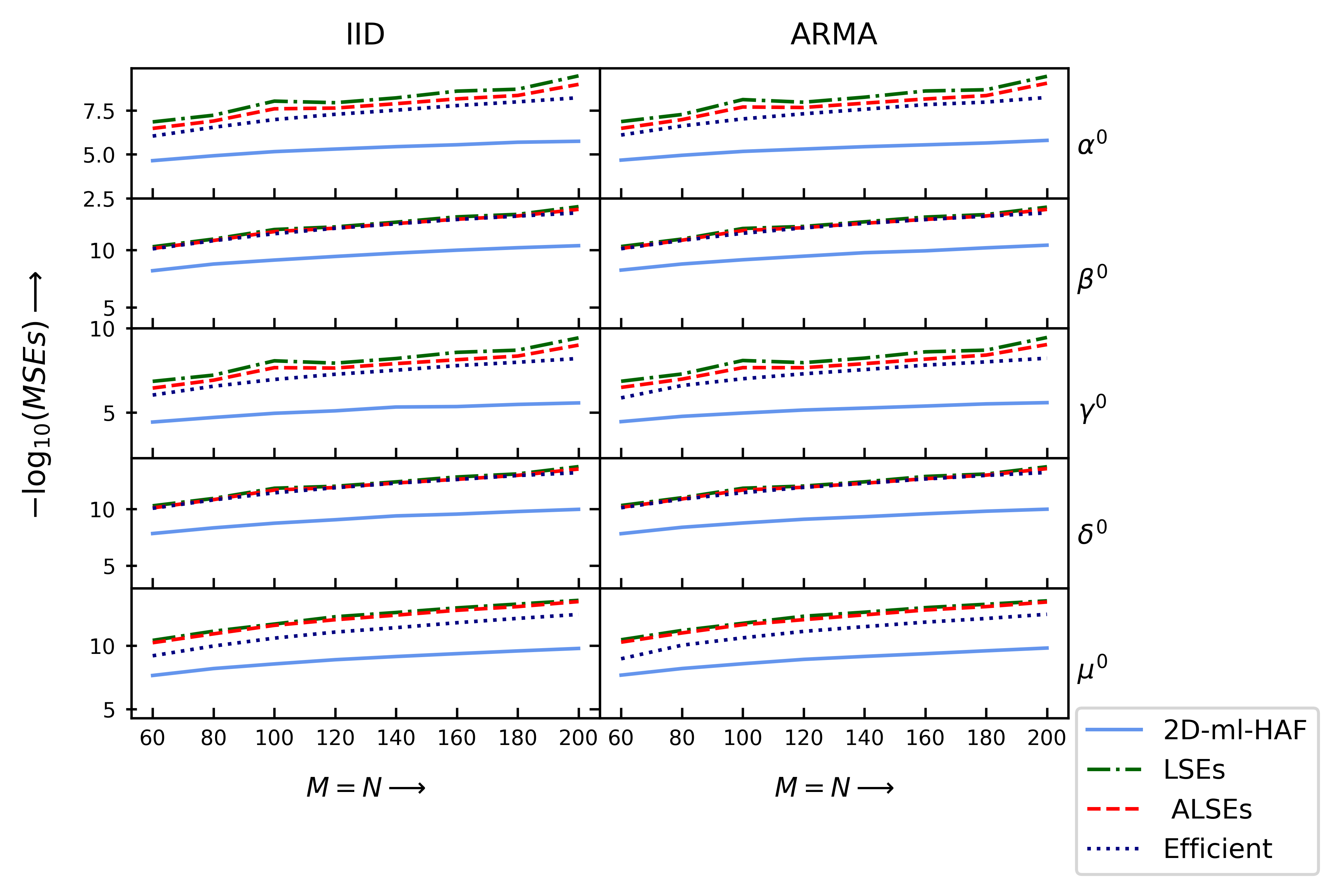
(a) Standard deviation of $\epsilon(m,n)$ is $\sigma=0.1$

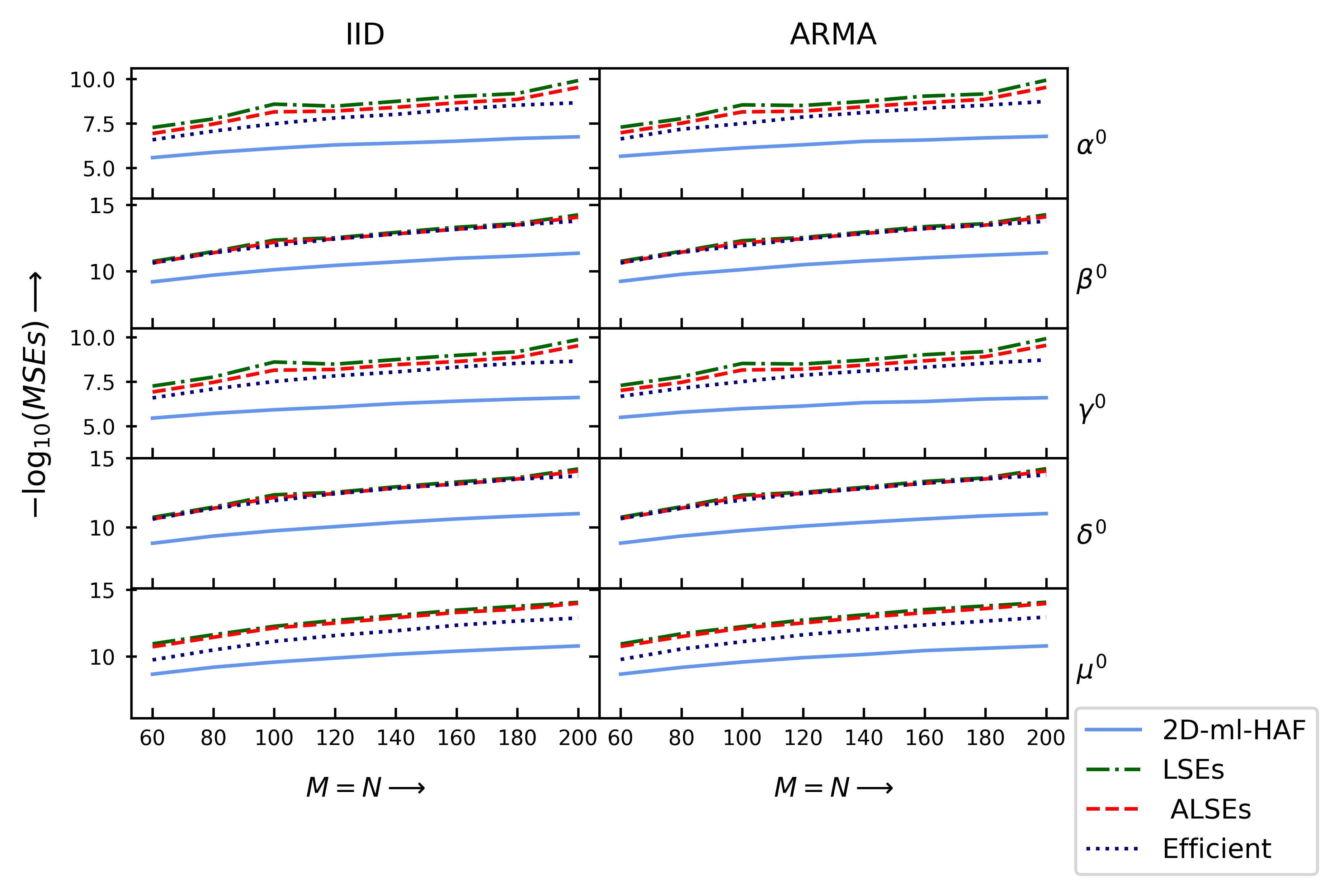
(b) Standard deviation of $\epsilon(m,n)$ is $\sigma=0.5$

Figure 1: Plots of $-\log(\mbox{MSEs})$ versus the sample size for estimators of non-linear parameters.

(a) Standard deviation of $\epsilon(m,n)$ is $\sigma=0.9$

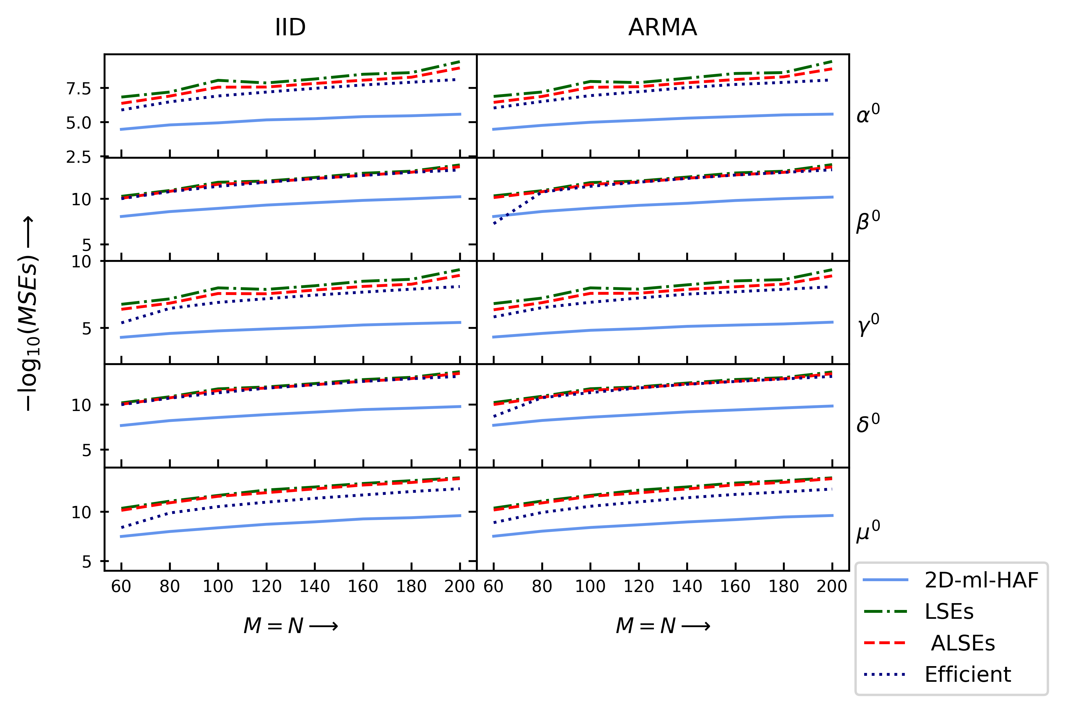
(b) Standard deviation of $\epsilon(m,n)$ is $\sigma=1$

Figure 2: Plots of $-\log(\mbox{MSEs})$ versus the sample size for estimators of non-linear parameters.

Table 1: Time and number of grid points taken to compute the estimates

Sample Size	Efficient		LSEs
$M=N$	Time(seconds)	Total No. of grid points	Time(seconds)	Number of grid points
2	0.044	12	0.128	27
3	0.041	96	0.308	2048
4	0.069	360	4.101	30375
5	0.119	960	34.609	221184
6	0.173	2100	198.038	1071875
7	0.250	4032	856.375	3981312

For the considered machine, it was not feasible to perform grid-search to get LSEs for more than $M=N=7$. When we plot sample size $M(=N)$ against the time to compute initial guess for LSEs, then it is observed to be linear. So, to get an idea of the time deviation of LSEs with that of proposed estimates at larger sample sizes, we predict time to obtain LSEs based on grid-search by fitting a simple linear regression model between $\log$ of sample size and $\log$ of time to get LSEs. From the results in Table 2, we can clearly observe the massive time difference of getting proposed estimates and LSEs. For example, if we go for sample size, say $M=N=40$, then it will take more than 20 years to obtain LSEs using grid-search over the same machine (even if we assume a large amount of RAM in a machine), while it took less than 10 minutes to obtain the proposed estimates.

Table 2: Comparing Time efficiency with Predicted time for LSEs

Sample Size	Efficient		LSEs
$M=N$	Computed Time	Total No. of grid points	Predicted Time	Number of grid points
8	0.530 sec	7.06E+03	32.165 min	1.23E+07
9	0.734 sec	1.15E+04	1.375 hr	3.28E+07
10	1.545 sec	1.78E+04	3.195 hr	7.86E+07
15	5.831 sec	9.41E+04	3.411 days	2.20E+09
20	26.479 sec	3.03E+05	34.070 days	2.29E+10
25	1.015 min	7.49E+05	203.051 days	1.40E+11
30	2.443 min	1.56E+06	2.392 yr	6.11E+11
35	5.369 min	2.91E+06	8.209 yr	2.12E+12
40	8.525 min	4.99E+06	23.888 yr	6.22E+12
45	14.530 min	8.02E+06	61.288 yr	1.61E+13
50	24.243 min	1.22E+07	142.37 yr	3.75E+13

4.3 Texture Pattern Estimation

2D-chirp signals create interesting gray-scale texture patterns. In order to analyze the effectiveness of the proposed estimators for estimating texture patterns accurately, we generate data from the complex counterpart of the model with same set of parameters as in (13). Then real and imaginary part of the obtained data is contaminated independently with i.i.d. normal errors having mean 0 and variance $\sigma^{2}=0.09$. The data matrix obtained is of size $100\times 100$. We analyze this data using the proposed estimator, the optimal LSEs, ALSEs, and also with the 2D-multilag-HAF method. Note that we have used true values as initial guess for obtaining optimal estimators, LSEs and ALSEs because of the computational complexity and grid-search method for obtaining 2D-multilag-HAF estimators and proposed estimators.
 
Plugging these estimators in the deterministic part of the model, we get estimated texture patterns as the real part of the reproduced data. We also present real part of the original dataset to compare the original and estimated textures. It is clear from the figures that texture pattern obtained using the proposed method is visually the same as that obtained using optimal LSEs and ALSEs, while the 2D-multilag-HAF estimator gives a slightly different pattern than the original one.

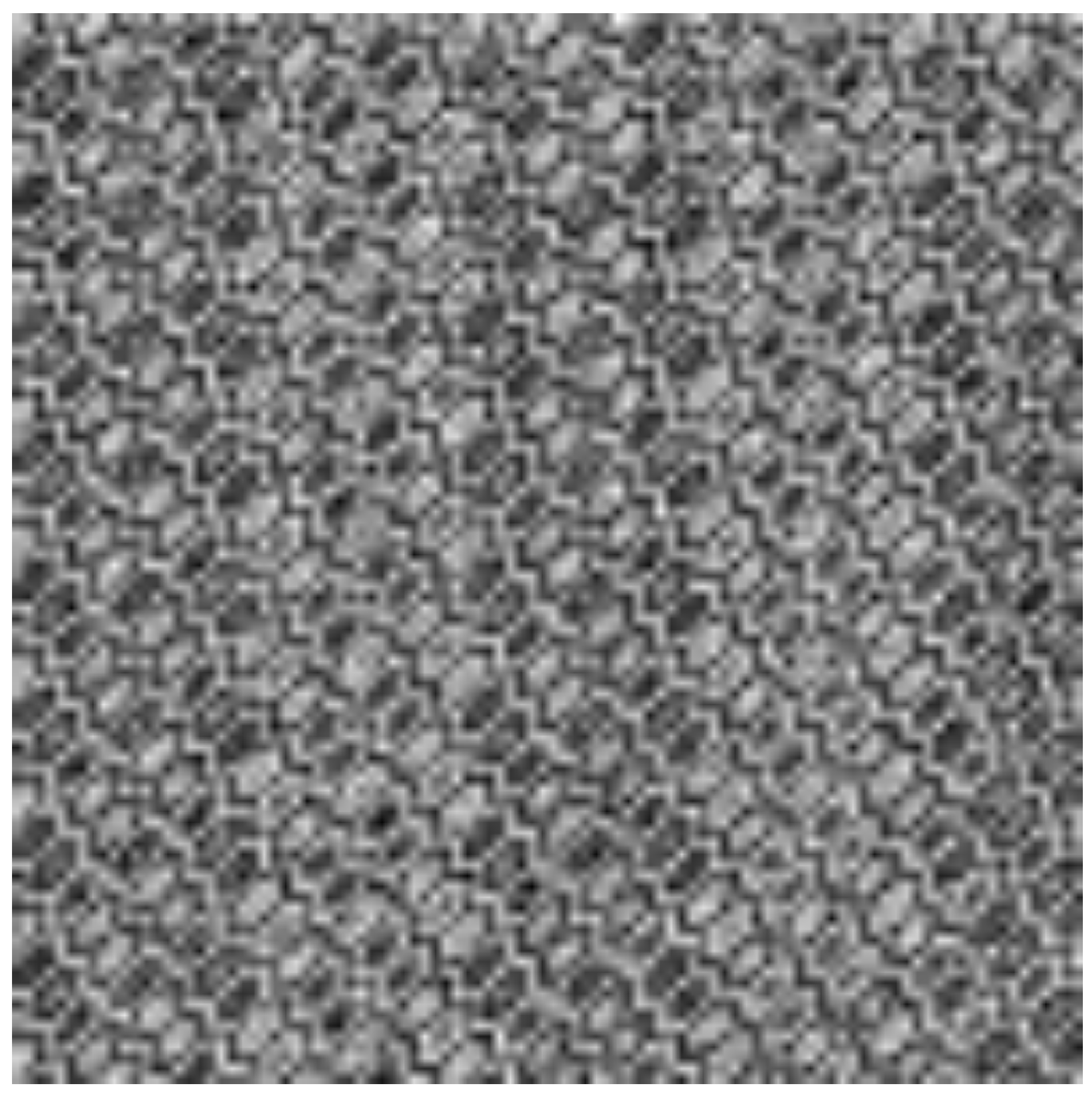
(a) Contaminated Texture

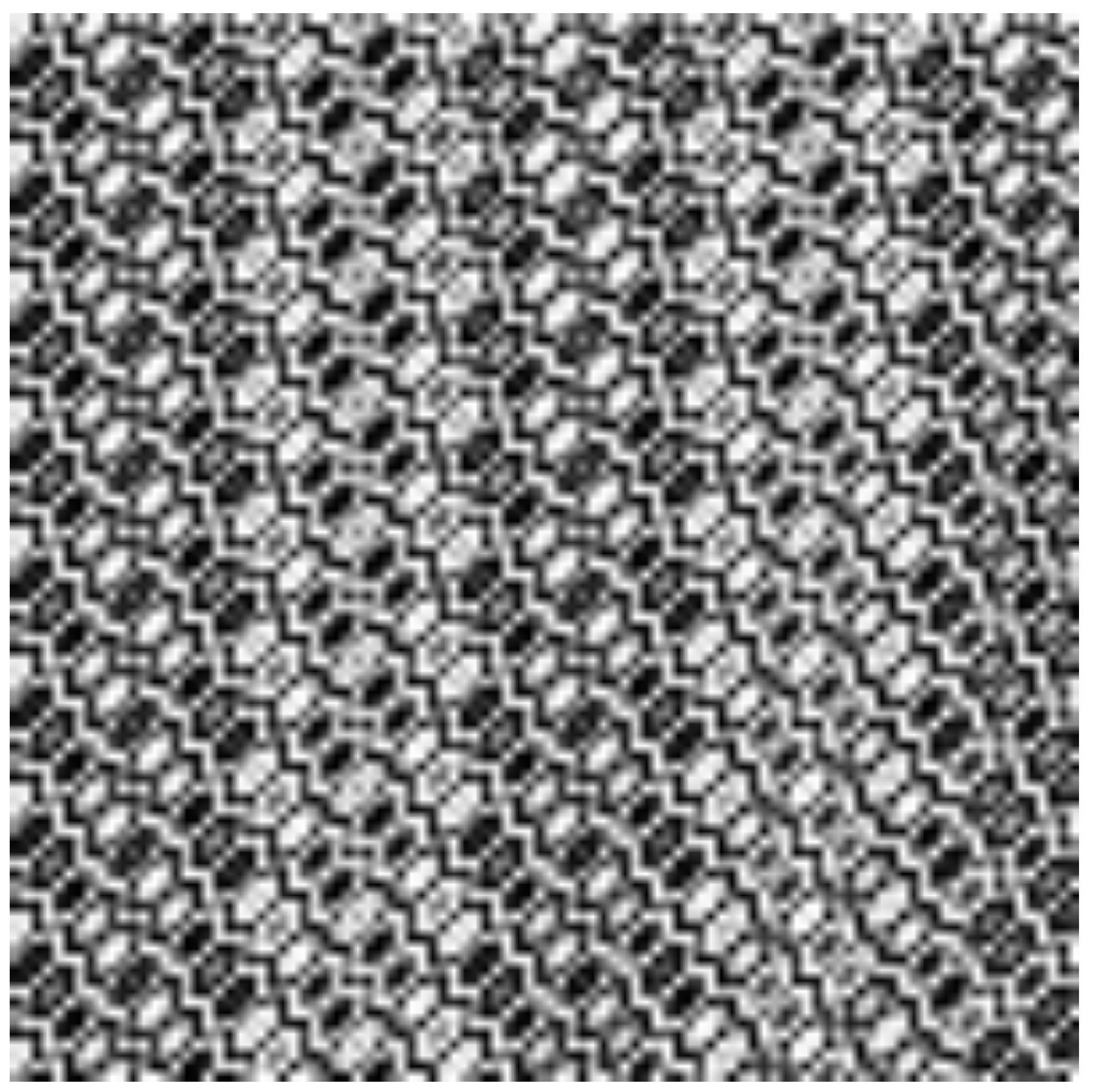
(b) Original Texture

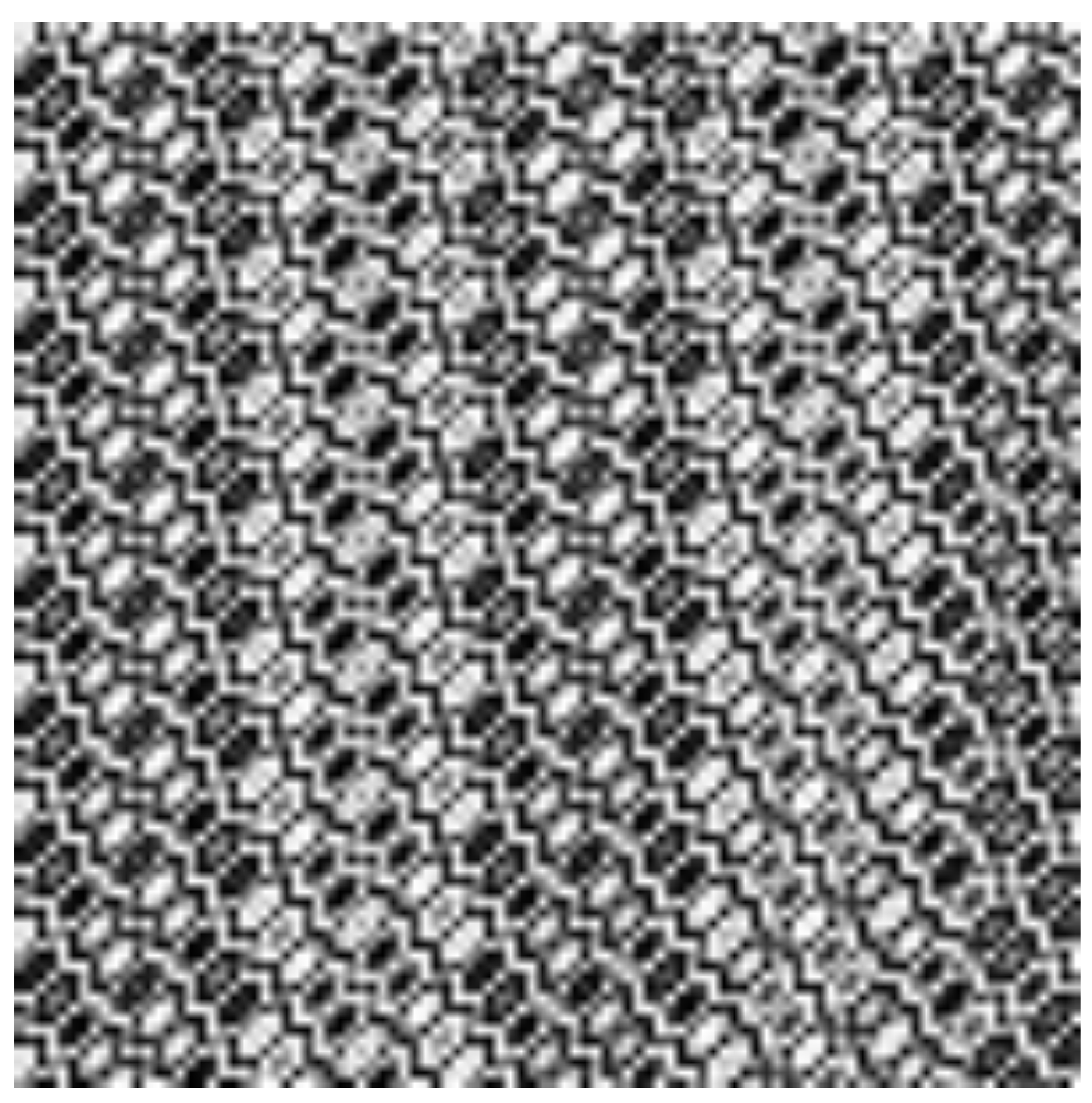
(c) Texture estimated
     using LSEs

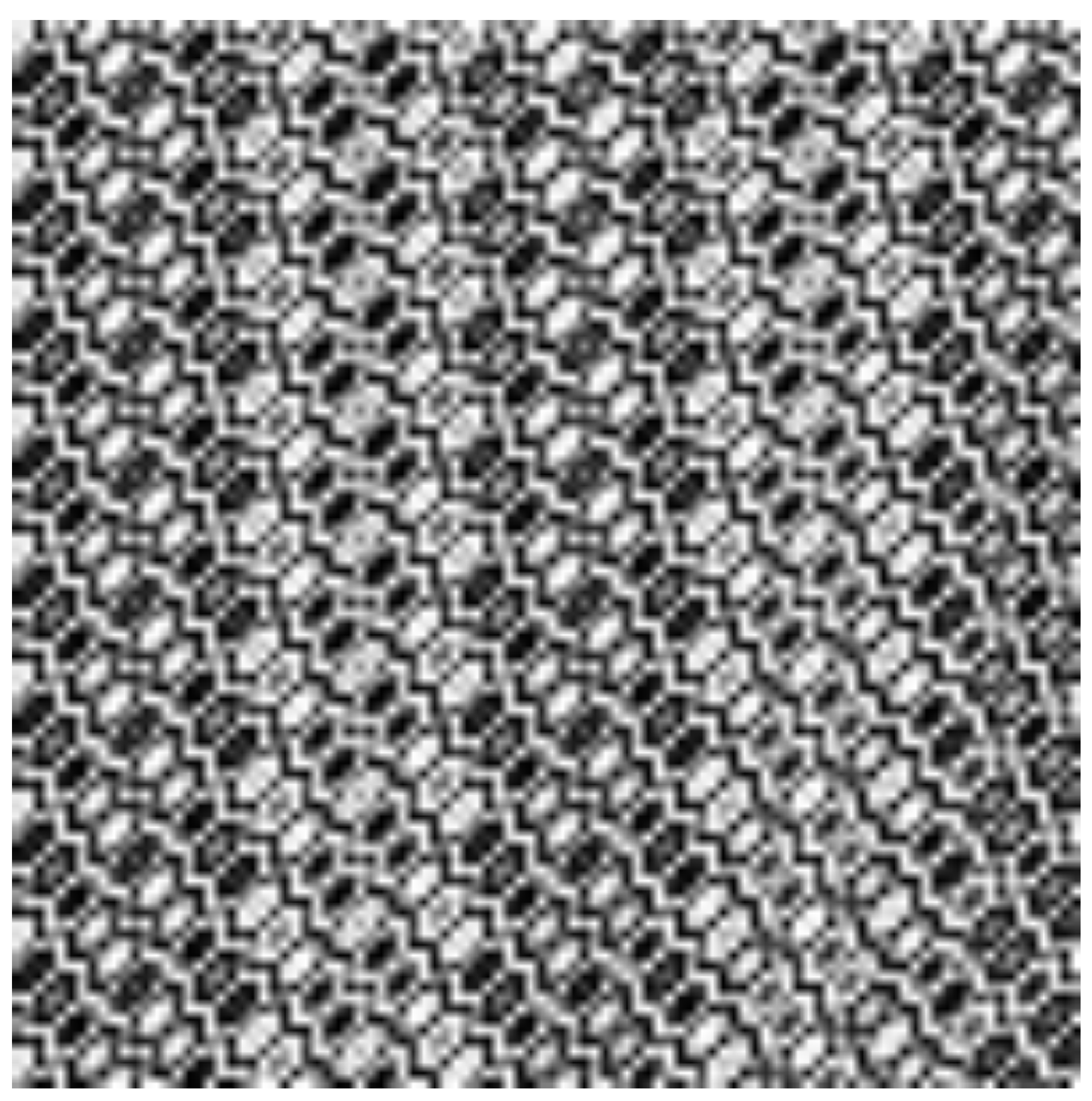
(d) Texture estimated
     using ALSEs

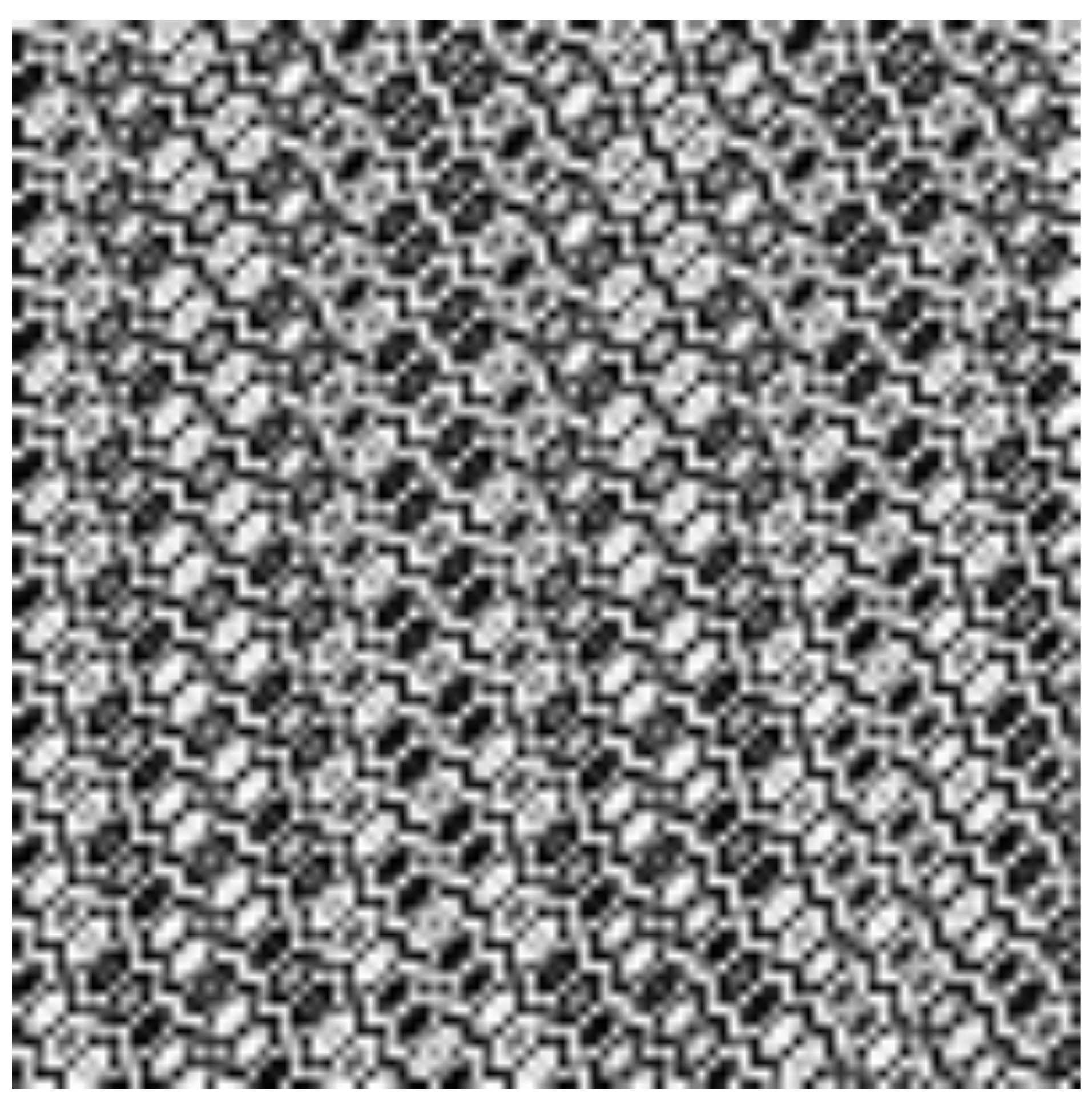
(e) Texture estimated
    using 2D-multilag-HAF
    method

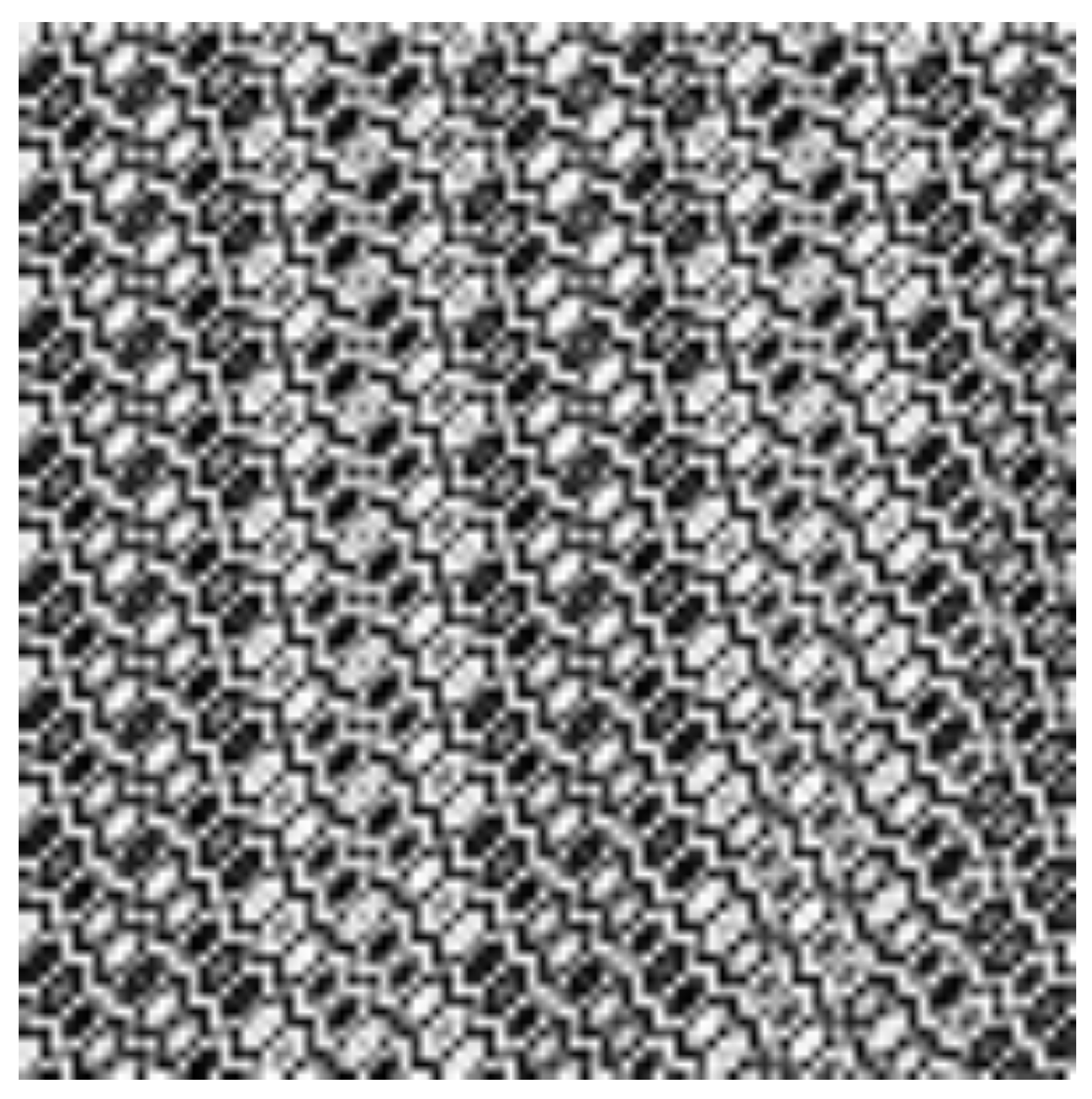
(f) Texture estimated
using proposed method

Figure 3: A comparison of estimated textures using LSEs, ALSEs, 2D-multilag-HAF and the proposed estimators.

5 Conclusion

The paper proposes a computationally efficient method that produces estimators having the same rate of convergence as the LSEs or ALSEs. The key idea is to develop a strategy by disintegrating the 2D model into several 1D chirp models and then design an optimal estimation method to obtain estimates of the 2D model. We believe that this idea can lead to several other computationally efficient algorithms which can be used to estimate higher order polynomial phase signals’ parameters also. The proposed estimators are not only asymptotically unbiased but also have an asymptotic normal distribution and same rate of convergence as that of the LSEs. Furthermore, the estimators converge strongly to the true value of the parameters. Extensive numerical simulations firmly support the theoretical results and also unveil the gigantic gap between time required for obtaining proposed estimates and the LSEs. Synthetic data analysis illustrates effectiveness of the proposed estimators to recover 2D gray-scale textures contaminated with noise.

Declarations

• Funding: Part of the work of the third author has been supported by a research grant from the Science and Engineering Research Board, Government of India.

• Conflict of interest/Competing interests (check journal-specific guidelines for which heading to use): Not applicable.

• Ethics approval: Not applicable.

• Consent to participate: Not applicable.

• Consent for publication: Not applicable.

• Availability of data and materials: Not applicable.

• Code availability: The authors can share the code used for simulations, on individual requests.

• Authors’ contributions: All authors contributed to study the conceptualization, methodology, review and editing. Formal analysis of proofs and simulations analysis were performed by Abhinek Shukla. The first draft of the manuscript was written by Abhinek Shukla and all authors commented on revising the previous versions of the manuscript. All authors read and approved the final manuscript. Amit Mitra and Debasis Kundu had supervised the whole research project.

Appendix A

Proof of Theorem 1: Given the data matrix $\bm{Y}$, we compute the LSEs of $\alpha^{0}+n_{0}\mu^{0}$ and $\beta^{0}$ corresponding to $n_{0}^{th}$ column vector of $\bm{Y}$. We denote the obtained estimators by $\widehat{\alpha}_{n_{0}}$ and $\widehat{\beta}_{n_{0}}$ to emphasize that these depend on $n_{0}$. Similarly, for fixed $m_{0}^{th}$ row of $\bm{Y}$, we have denoted the LSEs of $\gamma^{0}+m_{0}\mu^{0}$ and $\delta^{0}$ by $\widehat{\gamma}_{m_{0}}$ and $\widehat{\delta}_{m_{0}}$. Under assumptions that $X(m_{0},n_{0})$ are stationary (11) and (12), see [18], we have

$$\widehat{\beta}_{n_{0}} =\beta^{0}+o\bigg{(}\cfrac{1}{M^{2}}\bigg{)},\hskip 15.0pt\widehat{\alpha}_{n_{0}}=\alpha^{0}+n_{0}\mu^{0}+o\bigg{(}\cfrac{1}{M}\bigg{)},$$ (15)

$$\widehat{\gamma}_{m_{0}} =\gamma^{0}+m_{0}\mu^{0}+o\bigg{(}\cfrac{1}{N}\bigg{)},\hskip 15.0pt\widehat{\delta}_{m_{0}}=\delta^{0}+o\bigg{(}\cfrac{1}{N^{2}}\bigg{)}.$$ (16)

The final estimator of $\beta^{0}$ given by

$$\widehat{\beta}=\cfrac{\displaystyle\sum_{n_{0}=1}^{N}\widehat{\beta}_{n_{0}}}{N}$$

is strongly consistent estimate of $\beta^{0}$ which is observed by (15) and also that $\widehat{\beta}_{n_{0}}$ is strongly consistent for $\beta^{0}$ as $M\xrightarrow{}\infty$. For proof, one may refer to [15].
 
Similarly $\widehat{\delta}=\displaystyle\cfrac{1}{M}\sum_{m_{0}=1}^{M}\widehat{\delta}_{m_{0}}$ is strongly consistent estimator of $\delta^{0}$.
Denote $\bm{\tau}^{\top}=\begin{bmatrix}\makebox[0.0pt][l]{$\smash{\underbrace{\phantom{\begin{matrix}o\bigg{(}\cfrac{1}{M}\bigg{)}&\ldots&o\bigg{(}\cfrac{1}{M}\bigg{)}\end{matrix}}}_{\text{$\mbox{ $N$ times }$}}}$}o\bigg{(}\cfrac{1}{M}\bigg{)}&\ldots&o\bigg{(}\cfrac{1}{M}\bigg{)}&\makebox[0.0pt][l]{$\smash{\underbrace{\phantom{\begin{matrix}o\bigg{(}\cfrac{1}{N}\bigg{)}&\ldots&o\bigg{(}\cfrac{1}{N}\bigg{)}\end{matrix}}}_{\text{$\mbox{ $M$ times }$}}}$}o\bigg{(}\cfrac{1}{N}\bigg{)}&\ldots&o\bigg{(}\cfrac{1}{N}\bigg{)}\end{bmatrix}_{1\times(M+N)}.$
 
 
We now prove the consistency of the frequency parameter estimators $\widehat{\alpha},\widehat{\gamma}$, and that of $\widehat{\mu}$, estimator of the interaction term parameter. From (15) and (16), we have the following:

$$\begin{bmatrix}\widehat{\alpha}\\ l\widehat{\gamma}\\ \widehat{\mu}\end{bmatrix}=\Big{(}\bm{\Gamma}^{\top}\bm{\Gamma}\Big{)}^{-1}\bm{\Gamma}^{\top}\bm{\Lambda}=(\bm{\Gamma}^{\top}\bm{\Gamma})^{-1}\bm{\Gamma}^{\top}\bigg{(}\bm{\Gamma}\begin{bmatrix}\alpha^{0}\\ \gamma^{0}\\ \mu^{0}\end{bmatrix}+\bm{\tau}\bigg{)},\\$$ (17)

where $\bm{\Gamma}^{\top}=\begin{bmatrix}1&1&\cdots&1&0&0&\cdots&0\\ 0&0&\cdots&0&1&1&\cdots&1\\ 1&2&\cdots&N&1&2&\cdots&M\end{bmatrix}_{3\times(M+N)}$, and $\bm{\Lambda}^{\top}=\begin{bmatrix}\widehat{\alpha}_{1}&\widehat{\alpha}_{2}&\cdots&\widehat{\alpha}_{N}&\widehat{\gamma}_{1}&\widehat{\gamma}_{2}&\cdots&\widehat{\gamma}_{M}\end{bmatrix}$.
 
This implies that

$$\begin{bmatrix}\widehat{\alpha}\\ \widehat{\gamma}\\ \widehat{\mu}\end{bmatrix}=\begin{bmatrix}\alpha^{0}\\ \gamma^{0}\\ \mu^{0}\end{bmatrix}+(\bm{\Gamma}^{\top}\bm{\Gamma})^{-1}\begin{bmatrix}N\times o\bigg{(}\cfrac{1}{M}\bigg{)}\\ M\times o\bigg{(}\cfrac{1}{N}\bigg{)}\\ \cfrac{N(N+1)}{2}\times o\bigg{(}\cfrac{1}{M}\bigg{)}+\cfrac{M(M+1)}{2}\times o\bigg{(}\cfrac{1}{N}\bigg{)}\end{bmatrix}.$$ (18)

Now we look at the first element $a_{1}+a_{2}-a_{3}$ of the following matrix

$$(\bm{\Gamma}^{\top}\bm{\Gamma})^{-1}\begin{bmatrix}N\times o\bigg{(}\cfrac{1}{M}\bigg{)}\\ M\times o\bigg{(}\cfrac{1}{N}\bigg{)}\\ \cfrac{N(N+1)}{2}\times o\bigg{(}\cfrac{1}{M}\bigg{)}+\cfrac{M(M+1)}{2}\times o\bigg{(}\cfrac{1}{N}\bigg{)}\end{bmatrix}.$$

where,

$$a_{1} =\bigg{(}MK-\cfrac{M^{2}(M+1)^{2}}{4}\bigg{)}N\times o\bigg{(}\cfrac{1}{M}\bigg{)}/\Xi,$$

$$a_{2} =\cfrac{MN(M+1)(N+1)}{4}M\times o\bigg{(}\cfrac{1}{N}\bigg{)}/\Xi,$$

$$a_{3} =\cfrac{MN(N+1)}{2}\Bigg{(}\cfrac{N(N+1)}{2}\times o\bigg{(}\cfrac{1}{M}\bigg{)}+\cfrac{M(M+1)}{2}\times o\bigg{(}\cfrac{1}{N}\bigg{)}\Bigg{)}/\Xi,$$

and

$$\Xi=\cfrac{MN}{12}\bigg{(}N(N^{2}-1)+M(M^{2}-1)\bigg{)},K=\cfrac{N(N+1)(2N+1)}{6}+\cfrac{M(M+1)(2M+1)}{6}.$$

Now we look at $a_{1},a_{2}$ and $a_{3}$ individually and compute their limits.

$$a_{1} =\bigg{(}MK-\cfrac{M^{2}(M+1)^{2}}{4}\bigg{)}N\times o\bigg{(}\cfrac{1}{M}\bigg{)}/\Xi$$

$$=N\times\cfrac{o(1)}{\Xi}\times\bigg{(}\cfrac{N(N+1)(2N+1)}{6}+\cfrac{M(M+1)(M-1)}{12}\bigg{)}$$

$$=\cfrac{o(1)}{M}\times\cfrac{\bigg{(}2N(N+1)(2N+1)+M(M^{2}-1)\bigg{)}}{\bigg{(}N(N^{2}-1)+M(M^{2}-1)\bigg{)}}.$$

$\mbox{ This implies that }a_{1}\xrightarrow{a.s.}0\mbox{ as }\min\{M,N\}\rightarrow\infty.$ Here,

$$a_{2} =\cfrac{MN(M+1)(N+1)}{4}M\times o\bigg{(}\cfrac{1}{N}\bigg{)}/\Xi=o(1)\times\cfrac{M(M+1)}{\bigg{(}N(N^{2}-1)+M(M^{2}-1)\bigg{)}}.$$

$\mbox{ This implies that }a_{2}\xrightarrow{a.s.}0\mbox{ as }\min\{M,N\}\rightarrow\infty.$

$$a_{3} =\cfrac{MN(N+1)}{2}\Bigg{(}\cfrac{N(N+1)}{2}\times o\bigg{(}\cfrac{1}{M}\bigg{)}+\cfrac{M(M+1)}{2}\times o\bigg{(}\cfrac{1}{N}\bigg{)}\Bigg{)}/\Xi$$

$$=\cfrac{(N+1)}{2\Xi}\Bigg{(}N^{2}(N+1)\times o(1)+M^{2}(M+1)\times o(1)\Bigg{)}.$$

$\mbox{ This implies that }a_{3}\xrightarrow{a.s.}0\mbox{ as }\min\{M,N\}\rightarrow\infty.$ Hence, $\widehat{\alpha}$ is strongly consistent estimate of $\alpha^{0}$. Similarly strong consistency of $\widehat{\gamma}$ for $\gamma^{0}$ can be derived.
 
Now, the third element of $(\bm{\Gamma}^{\top}\bm{\Gamma})^{-1}\begin{bmatrix}N\times o\bigg{(}\cfrac{1}{M}\bigg{)}\\ M\times o\bigg{(}\cfrac{1}{N}\bigg{)}\\ \cfrac{N(N+1)}{2}\times o\bigg{(}\cfrac{1}{M}\bigg{)}+\cfrac{M(M+1)}{2}\times o\bigg{(}\cfrac{1}{N}\bigg{)}\end{bmatrix}$ can be written as $-b_{1}-b_{2}+b_{3}$, where

$$b_{1} =\cfrac{MN(N+1)}{2}\times N\times o\bigg{(}\cfrac{1}{M}\bigg{)}/\Xi=o(1)\cfrac{N(N+1)}{M\big{(}N(N^{2}-1)+M(M^{2}-1)\big{)}}.$$

$\mbox{ This implies that }b_{1}\xrightarrow{a.s.}0\mbox{ as }\min\{M,N\}\rightarrow\infty.$

$$b_{2} =\cfrac{NM(M+1)}{2}\times M\times o\bigg{(}\cfrac{1}{N}\bigg{)}/\Xi=o(1)\times\cfrac{M(M+1)}{N\big{(}N(N^{2}-1)+M(M^{2}-1)\big{)}}.$$

$\mbox{ This implies that }b_{2}\xrightarrow{a.s.}0\mbox{ as }\min\{M,N\}\rightarrow\infty.$

$$b_{3} =MN\times\bigg{(}\cfrac{N(N+1)}{2}\times o\bigg{(}\cfrac{1}{M}\bigg{)}+\cfrac{M(M+1)}{2}\times o\bigg{(}\cfrac{1}{N}\bigg{)}\bigg{)}/\Xi$$

$$=\bigg{(}\cfrac{N(N+1)}{\big{(}N(N^{2}-1)+M(M^{2}-1)\big{)}}\times o\bigg{(}\cfrac{1}{M}\bigg{)}+\cfrac{M(M+1)}{\big{(}N(N^{2}-1)+M(M^{2}-1)\big{)}}\times o\bigg{(}\cfrac{1}{N}\bigg{)}\bigg{)}.$$

Hence $b_{3}\xrightarrow{a.s.}0\mbox{ as }\min\{M,N\}\rightarrow\infty$. Hence, $\widehat{\mu}$ is a strongly consistent estimate of $\mu^{0}$. The strong consistency of estimators of amplitude parameters follows from the continuity mapping theorem.

Appendix B

Proof of Theorem 2: Suppose $\bm{\kappa}^{\top}=(A,B,\alpha,\beta)$ and
$\bm{\kappa}^{0^{\top}}=(A^{0}(n_{0}),B^{0}(n_{0}),\alpha^{0}+n_{0}\mu^{0},\beta^{0})$. We define sum of squares as follows:

$$Q_{n_{0}}(\bm{\kappa})=\displaystyle\sum_{m_{0}=1}^{M}\bigg{(}y(m_{0},n_{0})-A\cos(\alpha m_{0}+\beta m_{0}^{2})-B\sin(\alpha m_{0}+\beta m_{0}^{2})\bigg{)}^{2}.$$

Let $\widehat{\bm{\kappa}}$ be the minimizer of $Q_{n_{0}}(\bm{\kappa})$, then using Taylor Series expansion on the first derivative vector $Q_{n_{0}}^{\prime}(\bm{\kappa})$ around the point $\bm{\kappa}^{0}$, we get:

$$\bm{Q}_{n_{0}}^{\prime}(\widehat{\bm{\kappa}})-\bm{Q}_{n_{0}}^{\prime}(\bm{\kappa}^{0})=\bm{Q}_{n_{0}}^{\prime\prime}(\breve{\bm{\kappa}})(\widehat{\bm{\kappa}}-\bm{\kappa}^{0}),$$ (19)

where $\breve{\bm{\kappa}}$ is a point between $\widehat{\bm{\kappa}}$ and $\bm{\kappa}^{0}$. Also $\bm{Q}_{n_{0}}^{\prime}(\widehat{\bm{\kappa}})=0$ as $\widehat{\bm{\kappa}}$ is LSE of $\bm{\kappa}^{0}$.
Let us denote $\bm{D}_{1}^{-1}=diag(M^{1/2},M^{1/2},M^{3/2},M^{5/2})$. Then on multiplying $\bm{D}_{1}^{-1}$ both sides of equation (19), it gives:

$$-\big{[}\bm{D_{1}}\bm{Q}_{n_{0}}^{\prime\prime}(\breve{\bm{\kappa}})\bm{D_{1}}\big{]}^{-1}\bm{\Sigma}_{n_{0}}\displaystyle\bm{\Sigma}_{n_{0}}^{-1}\bm{D_{1}}\bm{Q}_{n_{0}}^{\prime}(\bm{\kappa}^{0}), =\bm{D_{1}}^{-1}(\widehat{\bm{\kappa}}-\bm{\kappa}^{0})$$ (20)

$$\mbox{where }\lim\limits_{M\rightarrow\infty}\big{[}\bm{D_{1}}\bm{Q}_{n_{0}}^{\prime\prime}(\breve{\bm{\kappa}})\bm{D_{1}}\big{]}^{-1}\bm{\Sigma}_{n_{0}} =I_{4\times 4},$$

and

$$\displaystyle\bm{\Sigma}_{n_{0}}^{-1}=\cfrac{2}{A^{0^{2}}+B^{0^{2}}}\begin{bmatrix}\cfrac{A^{0^{2}}(n_{0})+9B^{0^{2}}(n_{0})}{2}&-4A^{0}(n_{0})B^{0}(n_{0})&-18B^{0}(n_{0})&15B^{0}(n_{0})\\ -4A^{0}(n_{0})B^{0}(n_{0})&\cfrac{9A^{0^{2}}(n_{0})+B^{0^{2}}(n_{0})}{2}&18A^{0}(n_{0})&-15A^{0}(n_{0})\\ -18B^{0}(n_{0})&18A^{0}(n_{0})&96&-90\\ 15B^{0}(n_{0})&-15A^{0}(n_{0})&-90&90\end{bmatrix}.$$

The expression of $\bm{\Sigma}_{n_{0}}^{-1}$ can be obtained by proof of Theorem 2 shown in [15]. By using equation (20) and above expression of $\bm{\Sigma}_{n_{0}}^{-1}$, we get following asymptotically equivalent (a.e.) expression of the third element of vector $\bm{D_{1}}^{-1}(\widehat{\bm{\kappa}}-\bm{\kappa}^{0})$ as:

$$\begin{bmatrix}M^{3/2}\big{(}\widehat{\alpha}_{n_{0}}-(\alpha^{0}+n_{0}\mu^{0})\big{)}\end{bmatrix} \stackrel{{\scriptstyle\mathclap{\mbox{a.e.}}}}{{=}}\cfrac{4}{A^{0^{2}}+B^{0^{2}}}\Bigg{[}18\displaystyle\sum_{m}\cfrac{\eta(m_{0},n_{0})}{\sqrt{M}}-96\displaystyle\sum_{m_{0}}\cfrac{m_{0}\eta(m_{0},n_{0})}{M\sqrt{M}}+90\displaystyle\sum_{m_{0}}\cfrac{m_{0}^{2}\eta(m_{0},n_{0})}{M^{2}\sqrt{M}}\Bigg{]},$$ (21)

where, $\eta(m_{0},n_{0})=X(m_{0},n_{0})\big{(}A^{0}\sin\phi(m_{0},n_{0},\bm{\xi}^{0})-B^{0}\cos\phi(m_{0},n_{0},\bm{\xi}^{0})\big{)}$,
$\phi(m_{0},n_{0},\bm{\xi}^{0})=\alpha^{0}m_{0}+\beta^{0}m_{0}^{2}+\gamma^{0}n_{0}+\delta^{0}n_{0}^{2}+\mu^{0}m_{0}n_{0}$. We have used these notations for brevity. Similarly expressions of fourth, fifth and sixth element of $\bm{D_{1}}^{-1}(\widehat{\bm{\kappa}}-\bm{\kappa}^{0})$ can be written as in equations (22), (23) and (24) respectively:

$$\begin{bmatrix}M^{5/2}\big{(}\widehat{\beta}_{n_{0}}-\beta^{0}\big{)}\end{bmatrix} \stackrel{{\scriptstyle\mathclap{\mbox{a.e.}}}}{{=}}\cfrac{4}{A^{0^{2}}+B^{0^{2}}}\Bigg{[}-15\displaystyle\sum_{m_{0}}\cfrac{\eta(m_{0},n_{0})}{\sqrt{M}}+90\displaystyle\sum_{m_{0}}\cfrac{m_{0}\eta(m_{0},n_{0})}{M\sqrt{M}}-90\displaystyle\sum_{m_{0}}\cfrac{m_{0}^{2}\eta(m_{0},n_{0})}{M^{2}\sqrt{M}}\Bigg{]},$$ (22)

$$\begin{bmatrix}N^{3/2}\big{(}\widehat{\gamma}_{m_{0}}-(\gamma^{0}+m_{0}\mu^{0})\big{)}\end{bmatrix} \stackrel{{\scriptstyle\mathclap{\mbox{a.e.}}}}{{=}}\cfrac{4}{A^{0^{2}}+B^{0^{2}}}\Bigg{[}18\displaystyle\sum_{n_{0}}\cfrac{\eta(m_{0},n_{0})}{\sqrt{N}}-96\displaystyle\sum_{n_{0}}\cfrac{n_{0}\eta(m_{0},n_{0})}{N\sqrt{N}}+90\displaystyle\sum_{n_{0}}\cfrac{n_{0}^{2}\eta(m_{0},n_{0})}{N^{2}\sqrt{N}}\Bigg{]},$$ (23)

$$\begin{bmatrix}N^{5/2}\big{(}\widehat{\delta}_{m_{0}}-\delta^{0}\big{)}\end{bmatrix} \stackrel{{\scriptstyle\mathclap{\mbox{a.e.}}}}{{=}}\cfrac{4}{A^{0^{2}}+B^{0^{2}}}\Bigg{[}-15\displaystyle\sum_{n_{0}}\cfrac{\eta(m_{0},n_{0})}{\sqrt{N}}+90\displaystyle\sum_{n_{0}}\cfrac{n_{0}\eta(m_{0},n_{0})}{N\sqrt{N}}-90\displaystyle\sum_{n_{0}}\cfrac{n_{0}^{2}\eta(m_{0},n_{0})}{N^{2}\sqrt{N}}\Bigg{]}.$$ (24)

From equations (22) and (24) above, we can see that estimators $\widehat{\beta}$ and $\widehat{\delta}$ of $\beta^{0}$ and $\delta^{0}$ are asymptotically equivalent to the LSEs as they have same asymptotic variances by applying central limit theorem for stationary linear processes, see [10]. So now, remaining is to show asymptotic properties of estimators $(\widehat{\alpha},\widehat{\gamma},\widehat{\mu})^{\top}$.
 
The expression of proposed estimators of $(\alpha^{0},\gamma^{0},\mu^{0})^{\top}$ obtained is:

$$\begin{bmatrix}\widehat{\alpha}\\ \widehat{\gamma}\\ \widehat{\mu}\end{bmatrix}=\begin{bmatrix}\bigg{(}MK-\cfrac{M^{2}\big{(}M+1\big{)}^{2}}{4}\bigg{)}c_{\alpha}+\cfrac{MN(M+1)(N+1)}{4}c_{\gamma}-\cfrac{MN(N+1)}{2}c_{\alpha\gamma}\\ \leavevmode\nobreak\ \\ \cfrac{MN(M+1)(N+1)}{4}c_{\alpha}+\bigg{(}KN-\cfrac{N^{2}(N+1)^{2}}{4}\bigg{)}c_{\gamma}-\cfrac{NM(M+1)}{2}c_{\alpha\gamma}\\ \leavevmode\nobreak\ \\ -\cfrac{MN(N+1)}{2}c_{\alpha}-\cfrac{NM(M+1)}{2}c_{\gamma}+MNc_{\alpha\gamma}\end{bmatrix}/|\bm{\Gamma}^{\top}\bm{\Gamma}|,$$ (25)

$$c_{\alpha}=\displaystyle\sum_{n_{0}=1}^{N}\widehat{\alpha}_{n_{0}},c_{\gamma}=\displaystyle\sum_{m_{0}=1}^{M}\widehat{\gamma}_{m_{0}},c_{\alpha\gamma}=\displaystyle\sum_{n_{0}=1}^{N}n_{0}\widehat{\alpha}_{n_{0}}+\displaystyle\sum_{m_{0}=1}^{M}m_{0}\widehat{\gamma}_{m_{0}},$$

$$K=\cfrac{N(N+1)(2N+1)}{6}+\cfrac{M(M+1)(2M+1)}{6},\big{|}\bm{\Gamma}^{\top}\bm{\Gamma}\big{|}=\cfrac{MN}{12}\bigg{(}N(N^{2}-1)+M(M^{2}-1)\bigg{)}.$$

From (25), we get:

$$M^{3/2}N^{1/2}\big{(}\widehat{\alpha}-\alpha^{0}\big{)} =\bigg{(}\cfrac{2N(N+1)(2N+1)+M(M^{2}-1)}{N(N^{2}-1)+M(M^{2}-1)}\bigg{)}\cfrac{1}{\sqrt{N}}\displaystyle\sum_{n_{0}=1}^{N}M^{3/2}\big{(}\widehat{\alpha}_{n_{0}}-(\alpha^{0}+n_{0}\mu^{0})\big{)}$$

$$+\bigg{(}\cfrac{3M^{2}(M+1)}{N(N^{2}-1)+M(M^{2}-1)}\bigg{)}\cfrac{1}{\sqrt{M}}\displaystyle\sum_{m_{0}=1}^{M}N^{3/2}\big{(}\widehat{\gamma}_{m_{0}}-(\gamma^{0}+m_{0}\mu^{0})\big{)}$$

$$-\bigg{(}\cfrac{6M^{3/2}N^{1/2}(N+1)}{N(N^{2}-1)+M(M^{2}-1)}\bigg{)}\bigg{[}\displaystyle\sum_{n_{0}=1}^{N}n_{0}\big{(}\widehat{\alpha}_{n_{0}}-(\alpha^{0}+n_{0}\mu^{0})\big{)}$$

$$+\displaystyle\sum_{m_{0}=1}^{M}m_{0}\big{(}\widehat{\gamma}_{m_{0}}-(\gamma^{0}+m_{0}\mu^{0})\big{)}\bigg{]}.$$

For sufficiently large $M$ and $N$, we have:

$$M^{3/2}N^{1/2}\big{(}\widehat{\alpha}-\alpha^{0}\big{)} =\bigg{(}\cfrac{4N^{3}+M^{3}}{N^{3}+M^{3}}\bigg{)}\cfrac{1}{\sqrt{N}}\displaystyle\sum_{n_{0}=1}^{N}M^{3/2}\big{(}\widehat{\alpha}_{n_{0}}-(\alpha^{0}+n_{0}\mu^{0})\big{)}$$

$$+\bigg{(}\cfrac{3M^{3}}{N^{3}+M^{3}}\bigg{)}\cfrac{1}{\sqrt{M}}\displaystyle\sum_{m_{0}=1}^{M}N^{3/2}\big{(}\widehat{\gamma}_{m_{0}}-(\gamma^{0}+m_{0}\mu^{0})\big{)}$$

$$-\bigg{(}\cfrac{6N^{3}}{N^{3}+M^{3}}\bigg{)}\cfrac{1}{N^{3/2}}\displaystyle\sum_{n_{0}=1}^{N}n_{0}M^{3/2}\big{(}\widehat{\alpha}_{n_{0}}-(\alpha^{0}+n_{0}\mu^{0})\big{)}$$

$$-\bigg{(}\cfrac{6M^{3}}{N^{3}+M^{3}}\bigg{)}\cfrac{1}{M^{3/2}}\displaystyle\sum_{m_{0}=1}^{M}m_{0}N^{3/2}\big{(}\widehat{\gamma}_{m_{0}}-(\gamma^{0}+m_{0}\mu^{0})\big{)}.$$ (26)

Asymptotic normality of the estimators for $M=N\rightarrow\infty$ with given rates of convergence follows by applying central limit theorem for stationary processes [10].

We now present some important results which will be used to find the asymptotic variance-covariance matrix of the proposed estimators of non-linear parameters. Using equations (21) and (23) in the paper, we have the following observations:

1. $AsyVar\bigg{(}\cfrac{1}{2\sqrt{N}}\displaystyle\sum_{n_{0}=1}^{N}M^{3/2}\big{(}\widehat{\alpha}_{n_{0}}-(\alpha^{0}+n_{0}\mu^{0})\big{)}\bigg{)}=\cfrac{c\sigma^{2}96}{A^{0^{2}}+B^{0^{2}}}$,

2. $AsyVar\bigg{(}\cfrac{1}{2\sqrt{M}}\displaystyle\sum_{m_{0}=1}^{M}N^{3/2}\big{(}\widehat{\gamma}_{m_{0}}-(\gamma^{0}+m_{0}\mu^{0})\big{)}\bigg{)}=\cfrac{c\sigma^{2}96}{A^{0^{2}}+B^{0^{2}}}$,

3. $AsyVar\bigg{(}\cfrac{1}{2N^{3/2}}\displaystyle\sum_{n_{0}=1}^{N}n_{0}M^{3/2}\big{(}\widehat{\alpha}_{n_{0}}-(\alpha^{0}+n_{0}\mu^{0})\big{)}\bigg{)}=\cfrac{c\sigma^{2}32}{A^{0^{2}}+B^{0^{2}}}$,

4. $AsyVar\bigg{(}\cfrac{1}{2M^{3/2}}\displaystyle\sum_{m_{0}=1}^{M}m_{0}N^{3/2}\big{(}\widehat{\gamma}_{m_{0}}-(\gamma^{0}+m_{0}\mu^{0})\big{)}\bigg{)}=\cfrac{c\sigma^{2}32}{A^{0^{2}}+B^{0^{2}}}$,

5. $AsyCovar\bigg{(}\cfrac{1}{2\sqrt{N}}\displaystyle\sum_{n_{0}=1}^{N}M^{3/2}\big{(}\widehat{\alpha}_{n_{0}}-(\alpha^{0}+n_{0}\mu^{0})\big{)},\cfrac{1}{2\sqrt{M}}\displaystyle\sum_{m_{0}=1}^{M}N^{3/2}\big{(}\widehat{\gamma}_{m_{0}}-(\gamma^{0}+m_{0}\mu^{0})\big{)}\bigg{)}=0$,

6. $AsyCovar\bigg{(}\cfrac{1}{2\sqrt{N}}\displaystyle\sum_{n_{0}=1}^{N}M^{3/2}\big{(}\widehat{\alpha}_{n_{0}}-(\alpha^{0}+n_{0}\mu^{0})\big{)},\cfrac{1}{2N^{3/2}}\displaystyle\sum_{n_{0}=1}^{N}n_{0}M^{3/2}\big{(}\widehat{\alpha}_{n_{0}}-(\alpha^{0}+n_{0}\mu^{0})\big{)}\bigg{)}=\cfrac{c\sigma^{2}48}{A^{0^{2}}+B^{0^{2}}}$,

7. $AsyCovar\bigg{(}\cfrac{1}{2\sqrt{N}}\displaystyle\sum_{n_{0}=1}^{N}M^{3/2}\big{(}\widehat{\alpha}_{n_{0}}-(\alpha^{0}+n_{0}\mu^{0})\big{)},\cfrac{1}{2M^{3/2}}\displaystyle\sum_{m_{0}=1}^{M}m_{0}N^{3/2}\big{(}\widehat{\gamma}_{m_{0}}-(\gamma^{0}+m_{0}\mu^{0})\big{)}\bigg{)}=0$,

8. $AsyCovar\bigg{(}\cfrac{1}{2\sqrt{M}}\displaystyle\sum_{m_{0}=1}^{M}N^{3/2}\big{(}\widehat{\gamma}_{m_{0}}-(\gamma^{0}+m_{0}\mu^{0})\big{)},\cfrac{1}{2N^{3/2}}\displaystyle\sum_{n_{0}=1}^{N}n_{0}M^{3/2}\big{(}\widehat{\alpha}_{n_{0}}-(\alpha^{0}+n_{0}\mu^{0})\big{)}\bigg{)}=0$,

9. $AsyCovar\bigg{(}\cfrac{1}{2\sqrt{M}}\displaystyle\sum_{m_{0}=1}^{M}N^{3/2}\big{(}\widehat{\gamma}_{m_{0}}-(\gamma^{0}+m_{0}\mu^{0})\big{)},\cfrac{1}{2M^{3/2}}\displaystyle\sum_{m_{0}=1}^{M}m_{0}N^{3/2}\big{(}\widehat{\gamma}_{m_{0}}-(\gamma^{0}+m_{0}\mu^{0})\big{)}\bigg{)}=\cfrac{c\sigma^{2}48}{A^{0^{2}}+B^{0^{2}}}$,

10. $AsyCovar\bigg{(}\cfrac{1}{2N^{3/2}}\displaystyle\sum_{n_{0}=1}^{N}n_{0}M^{3/2}\big{(}\widehat{\alpha}_{n_{0}}-(\alpha^{0}+n_{0}\mu^{0})\big{)},\cfrac{1}{2M^{3/2}}\displaystyle\sum_{m_{0}=1}^{M}m_{0}N^{3/2}\big{(}\widehat{\gamma}_{m_{0}}-(\gamma^{0}+m_{0}\mu^{0})\big{)}\bigg{)}=\cfrac{c\sigma^{2}}{2(A^{0^{2}}+B^{0^{2}})}$.

 
where $c=\displaystyle{\sum_{i=-\infty}^{\infty}\sum_{j=-\infty}^{\infty}}a^{2}(i,j)$.
 
Using the above results in equation (Appendix B) from the paper, we get asymptotic variance-covariance matrix of
 
$\begin{bmatrix}M^{3/2}N^{1/2}(\widehat{\alpha}-\alpha^{0})\\ N^{3/2}M^{1/2}(\widehat{\gamma}-\gamma^{0})\\ M^{3/2}N^{3/2}(\widehat{\mu}-\mu^{0})\end{bmatrix}$ as: $\cfrac{c\sigma^{2}}{(A^{0^{2}}+B^{0^{2}})}\begin{bmatrix}996&612&-1224\\ 612&996&-1224\\ -1224&-1224&2448\end{bmatrix}.$
 
From (21), (22) and (23) equations of the paper, it is further observed that:

1. $AsyCovar\bigg{(}M^{5/2}N^{1/2}\big{(}\widehat{\beta}-\beta^{0}\big{)},M^{1/2}N^{5/2}\big{(}\widehat{\delta}-\delta^{0}\big{)}\bigg{)}=0$,

2. $AsyCovar\bigg{(}M^{5/2}N^{1/2}\big{(}\widehat{\beta}-\beta^{0}\big{)},\cfrac{1}{\sqrt{N}}\displaystyle\sum_{n_{0}=1}^{N}M^{3/2}\big{(}\widehat{\alpha}_{n_{0}}-(\alpha^{0}+n_{0}\mu^{0})\big{)}\bigg{)}=\cfrac{-360c\sigma^{2}}{A^{0^{2}}+B^{0^{2}}}$,

3. $AsyCovar\bigg{(}M^{5/2}N^{1/2}\big{(}\widehat{\beta}-\beta^{0}\big{)},\cfrac{1}{\sqrt{M}}\displaystyle\sum_{m_{0}=1}^{M}N^{3/2}\big{(}\widehat{\gamma}_{m_{0}}-(\gamma^{0}+m_{0}\mu^{0})\big{)}\bigg{)}=0$,

4. $AsyCovar\bigg{(}M^{5/2}N^{1/2}\big{(}\widehat{\beta}-\beta^{0}\big{)},\cfrac{1}{N\sqrt{N}}\displaystyle\sum_{n_{0}=1}^{N}M^{3/2}n_{0}\big{(}\widehat{\alpha}_{n_{0}}-(\alpha^{0}+n_{0}\mu^{0})\big{)}\bigg{)}=\cfrac{-180c\sigma^{2}}{A^{0^{2}}+B^{0^{2}}}$,

5. $AsyCovar\bigg{(}M^{5/2}N^{1/2}\big{(}\widehat{\beta}-\beta^{0}\big{)},\cfrac{1}{M\sqrt{M}}\displaystyle\sum_{m_{0}=1}^{M}m_{0}N^{3/2}\big{(}\widehat{\gamma}_{m_{0}}-(\gamma^{0}+m_{0}\mu^{0})\big{)}\bigg{)}=0.$

Similar results can be derived for $M^{1/2}N^{5/2}\big{(}\widehat{\delta}-\delta^{0}\big{)}$.
 
Asymptotic variance-covariance matrix of the proposed estimators of non-linear parameters is given by:

$$\cfrac{c\sigma^{2}}{(A^{0^{2}}+B^{0^{2}})}\begin{bmatrix}996&-360&612&0&-1224\\ -360&360&0&0&0\\ 612&0&996&-360&-1224\\ 0&0&-360&360&0\\ -1224&0&-1224&0&2448\end{bmatrix}.$$ (27)

Next, we derive the asymptotics of amplitude estimators, please recall that by using Taylor series expansion of $\cos\phi(m_{0},n_{0},\widehat{\bm{\xi}})$ around the point $\bm{\xi}^{0}$, we can write:

$$\cos\widehat{\phi}-\cos\phi^{0}=-\sin\breve{\phi}\big{(}\widehat{\bm{\xi}}-\bm{\xi}^{0}\big{)}^{\top}\begin{bmatrix}m_{0}\\ m_{0}^{2}\\ n_{0}\\ n_{0}^{2}\\ m_{0}n_{0}\end{bmatrix}.$$

For brevity, we have denoted $\cos\phi(m_{0},n_{0},\widehat{\bm{\xi}})$ by $\cos\widehat{\phi}$, $\cos\phi(m_{0},n_{0},\widehat{\bm{\xi}})$ by $\cos\phi^{0}$, and $\sin\phi(m_{0},n_{0},\breve{\bm{\xi}})$ by $\sin\breve{\phi}$ , where $\breve{\bm{\xi}}$ is a point lying between $\widehat{\bm{\xi}}$ and $\bm{\xi}^{0}$.
 
Now consider first element of the following vector,

$$\sqrt{MN}\Bigg{(}\begin{bmatrix}\cfrac{2}{{MN}}\displaystyle\sum_{m_{0}=1}^{M}\sum_{n_{0}=1}^{N}y(m_{0},n_{0})\cos\widehat{\phi}\\ \cfrac{2}{{MN}}\displaystyle\sum_{m_{0}=1}^{M}\sum_{n_{0}=1}^{N}y(m_{0},n_{0})\sin\widehat{\phi}\end{bmatrix}-\begin{bmatrix}A^{0}\\ B^{0}\end{bmatrix}\Bigg{)},$$

we get:

$$\sqrt{MN}\bigg{(}\cfrac{2}{{MN}}\displaystyle\sum_{m_{0}=1}^{M}\sum_{n_{0}=1}^{N}y(m_{0},n_{0})\cos{\phi^{0}}-\cfrac{2}{{MN}}\displaystyle\sum_{m_{0}=1}^{M}\sum_{n_{0}=1}^{N}y(m_{0},n_{0})\sin{\breve{\phi}}R(m_{0},n_{0})-A^{0}\bigg{)},$$ (28)

where $R(m_{0},n_{0})=\big{(}\widehat{\bm{\xi}}-\bm{\xi}^{0}\big{)}^{\top}\begin{bmatrix}m_{0}\\ m_{0}^{2}\\ n_{0}\\ n_{0}^{2}\\ m_{0}n_{0}\end{bmatrix}$, and second element of the above amplitude vector can be written as:

$$\sqrt{MN}\bigg{(}\cfrac{2}{{MN}}\displaystyle\sum_{m_{0}=1}^{M}\sum_{n_{0}=1}^{N}y(m_{0},n_{0})\sin{\phi^{0}}+\cfrac{2}{{MN}}\displaystyle\sum_{m_{0}=1}^{M}\sum_{n_{0}=1}^{N}y(m_{0},n_{0})\sin{\breve{\phi}}R(m_{0},n_{0})-B^{0}\bigg{)}.$$ (29)

Now let us look at the first and the last term of equation (28) and putting value of $y(m_{0},n_{0})$ from the model (1),

$$\sqrt{MN}\bigg{(}\cfrac{2}{{MN}}\displaystyle\sum_{m_{0}=1}^{M}\sum_{n_{0}=1}^{N}y(m_{0},n_{0})\cos{\phi^{0}}-A^{0}\bigg{)}$$

$$=\sqrt{MN}\bigg{(}\cfrac{2}{{MN}}\displaystyle\sum_{m_{0}=1}^{M}\sum_{n_{0}=1}^{N}A^{0}\cos^{2}\phi^{0}-A^{0}+\cfrac{2}{{MN}}\displaystyle\sum_{m_{0}=1}^{M}\sum_{n_{0}=1}^{N}B^{0}\sin\phi^{0}\cos\phi^{0}+\cfrac{2}{{MN}}\displaystyle\sum_{m_{0}=1}^{M}\sum_{n_{0}=1}^{N}X(m_{0},n_{0})\cos\phi^{0}\bigg{)}$$

$$\stackrel{{\scriptstyle\mathclap{\mbox{a.e.}}}}{{=}}\cfrac{2}{\sqrt{MN}}\displaystyle\sum_{m_{0}=1}^{M}\sum_{n_{0}=1}^{N}X(m_{0},n_{0})\cos\phi^{0}.$$ (30)

The above result has been obtained from a famous number theory conjecture by [17].
In second term of (28), $R(m_{0},n_{0})$ is a sum of five terms, so now consider first term of
$\cfrac{2}{{MN}}\displaystyle\sum_{m_{0}=1}^{M}\sum_{n_{0}=1}^{N}y(m_{0},n_{0})\sin{\breve{\phi}}R(m_{0},n_{0})$,

$$\cfrac{2}{{\sqrt{MN}}}\displaystyle\sum_{m_{0}=1}^{M}\sum_{n_{0}=1}^{N}y(m_{0},n_{0})\sin{\breve{\phi}}m_{0}(\widehat{\alpha}-\alpha^{0})$$

$$=\cfrac{2}{{\sqrt{MN}}}\displaystyle\sum_{m_{0}=1}^{M}\sum_{n_{0}=1}^{N}A^{0}\cos\phi^{0}\sin{\breve{\phi}}m_{0}(\widehat{\alpha}-\alpha^{0})+\cfrac{2}{{\sqrt{MN}}}\displaystyle\sum_{m_{0}=1}^{M}\sum_{n_{0}=1}^{N}B^{0}\sin\phi^{0}\sin{\breve{\phi}}m_{0}(\widehat{\alpha}-\alpha^{0})$$

$$+\cfrac{2}{{\sqrt{MN}}}\displaystyle\sum_{m_{0}=1}^{M}\sum_{n_{0}=1}^{N}X(m_{0},n_{0})\sin{\breve{\phi}}m_{0}(\widehat{\alpha}-\alpha^{0})$$

$$=\bigg{(}\cfrac{2}{{{M^{2}N}}}\displaystyle\sum_{m_{0}=1}^{M}\sum_{n_{0}=1}^{N}A^{0}\cos\phi^{0}\sin{\breve{\phi}}m_{0}\bigg{)}M\sqrt{MN}(\widehat{\alpha}-\alpha^{0})+$$

$$\hskip 20.0pt\bigg{(}\cfrac{2}{{{M^{2}N}}}\displaystyle\sum_{m_{0}=1}^{M}\sum_{n_{0}=1}^{N}B^{0}\sin\phi^{0}\sin{\breve{\phi}}m_{0}\bigg{)}M\sqrt{MN}(\widehat{\alpha}-\alpha^{0})+$$

$$\hskip 20.0pt\bigg{(}\cfrac{2}{{{M^{2}N}}}\displaystyle\sum_{m_{0}=1}^{M}\sum_{n_{0}=1}^{N}X(m_{0},n_{0})\sin{\breve{\phi}}m_{0}\bigg{)}M\sqrt{MN}(\widehat{\alpha}-\alpha^{0})$$

$$\stackrel{{\scriptstyle\mathclap{\mbox{a.e.}}}}{{=}}\bigg{(}\cfrac{2}{{{M^{2}N}}}\displaystyle\sum_{m_{0}=1}^{M}\sum_{n_{0}=1}^{N}B^{0}\sin\phi^{0}\sin{\breve{\phi}}m_{0}\bigg{)}M\sqrt{MN}(\widehat{\alpha}-\alpha^{0}),\mbox{\hskip 20.0ptby using Proposition 1 of \cite[cite]{[\@@bibref{}{Lahiri_2017}{}{}]}.}$$

So, finding the asymptotic distribution of (28) boils down to finding asymptotic distribution of

$$\cfrac{2}{\sqrt{MN}}\displaystyle\sum_{m_{0}=1}^{M}\sum_{n_{0}=1}^{N}X(m_{0},n_{0})\cos\phi^{0}-\bigg{(}\cfrac{2}{{\sqrt{MN}}}\displaystyle\sum_{m_{0}=1}^{M}\sum_{n_{0}=1}^{N}B^{0}\sin\phi^{0}\sin{\breve{\phi}}\bigg{)}R(m_{0},n_{0}),$$

which is further asymptotically equivalent to:

$$\cfrac{2}{\sqrt{MN}}\displaystyle\sum_{m_{0}=1}^{M}\sum_{n_{0}=1}^{N}X(m_{0},n_{0})\cos\phi^{0}-B^{0}\bigg{(}\cfrac{1}{2}M^{3/2}N^{1/2}(\widehat{\alpha}-\alpha^{0})+\cfrac{1}{3}M^{5/2}N^{1/2}(\widehat{\beta}-\beta^{0})$$

$$+\cfrac{1}{2}N^{3/2}M^{1/2}(\widehat{\gamma}-\gamma^{0})+\cfrac{1}{3}N^{5/2}M^{1/2}(\widehat{\delta}-\delta^{0})+\cfrac{1}{4}M^{3/2}N^{3/2}(\widehat{\mu}-\mu^{0})\bigg{)}.$$ (31)

Asymptotic normality of amplitude estimators is thus proved by equation (Appendix B). Now we need to derive the expression of their asymptotic variances.
 
After lengthy calculations, we get the asymptotic variance of $\widehat{A}$ as follows:

$$\cfrac{c\sigma^{2}}{(A^{0^{2}}+B^{0^{2}})}(2A^{0^{2}}+187B^{0^{2}}).$$

Similarly by calculating other terms too, we get complete variance co-variance matrix $\bm{\Sigma}$ as mentioned in Theorem 2.
 
Hence the result.

References

- [1] Barbarossa, S., Scaglione, A., & Giannakis, G. B. (1998). Product high-order ambiguity function for multicomponent polynomial-phase signal modeling. In IEEE Transactions on Signal Processing, vol. 46, no. 3, pp. 691-708.
- [2] Barbarossa, S., Di Lorenzo, P., & Vecchiarelli, P. (2014). Parameter estimation of 2D multi-component polynomial phase signals: an application to SAR imaging of moving targets. IEEE Transactions on Signal Processing, 62(17), 4375-4389.
- [3] Djurović, I., Wang, P., & Ioana, C. (2010). Parameter estimation of 2-D cubic phase signal using cubic phase function with genetic algorithm. Signal Processing, 90(9), 2698-2707.
- [4] Djurović, I., & Stanković, L. (2014). Quasi-maximum-likelihood estimator of polynomial phase signals. IET Signal Processing, 8(4), 347-359.
- [5] Djurović, I. (2017). Quasi ML algorithm for 2-D PPS estimation. Multidimensional Systems and Signal Processing, 28(2), 371-387.
- [6] Francos, J. M., & Friedlander, B. (1995, October). The polynomial phase difference operator for modeling of nonhomogeneous images. In Proceedings., International Conference on Image Processing (Vol. 2, pp. 276-279). IEEE.
- [7] Friedlander, B., & Francos, J. M. (1996). Model based phase unwrapping of 2-D signals. IEEE Transactions on Signal Processing, 44(12), 2999-3007.
- [8] Francos, J. M., & Friedlander, B. (1998). Two-dimensional polynomial phase signals: Parameter estimation and bounds. Multidimensional Systems and Signal Processing, 9(2), 173-205.
- [9] Francos, J. M., & Friedlander, B. (1999). Parameter estimation of 2-D random amplitude polynomial-phase signals. IEEE transactions on signal processing, 47(7), 1795-1810.
- [10] Fuller, W. A. (1996). Introduction to Statistical Time Series, second Edition, John Wiley and Sons, New York.
- [11] Grover, R., Kundu, D.,& Mitra, A. (2018). Approximate least squares estimators of a two-dimensional Chirp model and their asymptotic properties. Journal of Multivariate Analysis, 168, 211-220.
- [12] Grover, R., Kundu, D., & Mitra, A. (2021). An efficient methodology to estimate the parameters of a two-dimensional Chirp signal model. Multidimensional Systems and Signal Processing, 32(1), 49-75.
- [13] Guo, Y., & Li, B. Z. (2018). Novel method for parameter estimation of Newton’s rings based on CFRFT and ER-WCA. Signal Processing, 144, 118-126.
- [14] Lahiri, A., Kundu, D., & Mitra, A. (2013). Efficient algorithm for estimating the parameters of two dimensional Chirp signal. Sankhya B, 75(1), 65-89.
- [15] Lahiri, A., Kundu, D., & Mitra, A. (2015). Estimating the parameters of multiple chirp signals. Journal of Multivariate Analysis, 139, 189-206.
- [16] Lahiri, A., & Kundu, D. (2017). On parameter estimation of two-dimensional polynomial phase signal model. Statistica Sinica, 1779-1792.
- [17] Montgomery, H. L. (1994). Ten lectures on the interface between analytic number theory and harmonic analysis (No. 84). American Mathematical Soc..
- [18] Nandi, S., & Kundu, D. (2004). Asymptotic properties of the least squares estimators of the parameters of the chirp signals. Annals of the Institute of Statistical Mathematics, 56(3), 529-544.
- [19] O’shea, P. (2002). A new technique for instantaneous frequency rate estimation. IEEE Signal Processing Letters, 9(8), 251-252.
- [20] Peleg, S., & Porat, B. (1991). Estimation and classification of polynomial-phase signals. IEEE Transactions on Information Theory, 37(2), 422-430.
- [21] Wu, Y., So, H. C., & Liu, H. (2008). Subspace-based algorithm for parameter estimation of polynomial phase signals. IEEE Transactions on Signal Processing, 56(10), 4977-4983.
- [22] Zhang, K., Wang, S., & Cao, F. (2008, May). Product cubic phase function algorithm for estimating the instantaneous frequency rate of multicomponent two-dimensional Chirp signals. In 2008 Congress on image and signal processing (Vol. 5, pp. 498-502). IEEE.
- [23] Zhang, Y., Mobasseri, B. G., Dogahe, B. M., & Amin, M. G. (2010). Image-adaptive watermarking using 2D Chirps. Signal, Image and Video Processing, 4(1), 105-121.