Reduced symplectic homology and the secondary continuation map

Abstract.

We introduce the notion of a Weinstein domain with strongly $R$-essential skeleton and study a reduced version of symplectic homology in this context. In the open string case we introduce the notion of a strongly $R$-essential Lagrangian submanifold and study a reduced version of wrapped Floer homology. These reduced homologies provide a common domain of definition for the pair-of-pants product and for pair-of-pants secondary coproducts, which combine into the structure of a unital infinitesimal anti-symmetric bialgebra. The coproducts on reduced homology depend on choices, and this dependence is controlled by secondary continuation maps. Reduced homology and cohomology provide splittings of Rabinowitz Floer homology which are compatible with the products and the coproducts. These splittings also depend on choices, in the same way as the coproducts. We provide sufficient conditions under which the secondary continuation maps vanish, giving rise to canonical coproducts and splittings.

1. Introduction

The initial motivation for this paper lies in string topology. Given a closed orientable manifold $M$ of dimension $n$, denote $\Lambda=\Lambda M$ its free loop space, $\Lambda_{0}\subset\Lambda$ the subspace of constant loops, ${\mathbb{H}}_{*}\Lambda=H_{*+n}\Lambda$ the degree shifted loop homology and ${\mathbb{H}}^{*}\Lambda=H^{*+n}\Lambda$ the degree shifted loop cohomology of $M$. Chas and Sullivan [1] constructed the loop product $\mu:{\mathbb{H}}_{*}\Lambda\otimes{\mathbb{H}}_{*}\Lambda\to{\mathbb{H}}_{*}\Lambda$ of shifted degree $0$, and Sullivan [13] and Goresky-Hingston [11] constructed the loop coproduct $\lambda:{\mathbb{H}}_{*}(\Lambda,\Lambda_{0})\to{\mathbb{H}}_{*}(\Lambda,\Lambda_{0})\otimes{\mathbb{H}}_{*}(\Lambda,\Lambda_{0})$ (with coefficients in a field) of shifted degree $1-2n$, respectively the algebraically dual cohomology product $\lambda^{\vee}:{\mathbb{H}}^{*}(\Lambda,\Lambda_{0})\otimes{\mathbb{H}}^{*}(\Lambda,\Lambda_{0})\to{\mathbb{H}}^{*}(\Lambda,\Lambda_{0})$ of shifted degree $2n-1$ (with arbitrary coefficients). Very quickly the question arose as to whether it is possible to find a common domain of definition for the product and the coproduct, motivated in particular by the following relation conjectured by Sullivan:

(1) $$\lambda\mu=(\mu\otimes 1)(1\otimes\lambda)+(1\otimes\mu)(\lambda\otimes 1).$$

We gave in [4] one answer to this question, replacing ${\mathbb{H}}_{*}\Lambda$ by the Rabinowitz loop homology $\widehat{{\mathbb{H}}}_{*}\Lambda$, which is a homology group of Tate flavor consisting roughly of one copy of the loop homology and one copy of the loop cohomology, where both $\mu$ and $\lambda$ admit extensions which fit into the structure of a graded Frobenius algebra satisfying Poincaré duality [5]. It is the purpose of this paper to give a different answer to this question, replacing ${\mathbb{H}}_{*}\Lambda$ with reduced loop homology $\overline{{\mathbb{H}}}_{*}\Lambda$. This is a homology group lying between ${\mathbb{H}}_{*}\Lambda$ and ${\mathbb{H}}_{*}(\Lambda,\Lambda_{0})$ in the sense that the canonical projection from the first to the second factors as ${\mathbb{H}}_{*}\Lambda\to\overline{{\mathbb{H}}}_{*}\Lambda\to{\mathbb{H}}_{*}(\Lambda,\Lambda_{0})$. As such, reduced loop homology is much smaller than Rabinowitz loop homology and admits a direct geometric description. The product $\mu$ on ${\mathbb{H}}_{*}\Lambda$ descends to a canonical product $\bar{\mu}$ on $\overline{{\mathbb{H}}}_{*}\Lambda$, and the coproduct $\lambda$ extends to a coproduct $\bar{\lambda}$ on the same domain. The extension $\bar{\lambda}$ is canonical provided $H_{1}(M)=0$, but otherwise it may depend on choices. These two operations fit together into the structure of a unital infinitesimal anti-symmetric bialgebra as defined in [5]. In particular, the following unital form of Sullivan’s relation is satisfied, where we denote $\bar{\eta}$ the unit for the product $\bar{\mu}$:

(2) $$\bar{\lambda}\bar{\mu}=(\bar{\mu}\otimes 1)(1\otimes\bar{\lambda})+(1\otimes\bar{\mu})(\bar{\lambda}\otimes 1)-(\bar{\mu}\otimes\bar{\mu})(1\otimes\bar{\lambda}\bar{\eta}\otimes 1).$$

As shown in §9, the term $\bar{\lambda}\bar{\eta}$ can be nonzero in some examples, and zero in others. This topic is discussed in more detail in [3].

As a matter of fact, we discuss in this paper a more general symplectic situation. Namely, we exhibit the class of strongly $R$-essential Weinstein domains $W$ (Definition 2.1) of dimension $2n$, where $R$ is a principal ideal domain. For such Weinstein domains we can define the (degree shifted) reduced symplectic homology $\overline{S{\mathbb{H}}}_{*}(W)=\overline{SH}_{*+n}(W)$. This class of Weinstein domains includes in particular disc cotangent bundles, in which case reduced symplectic homology is a model for reduced loop homology. Reduced symplectic homology features the same properties as those of reduced loop homology above: it lies between symplectic homology $S{\mathbb{H}}_{*}(W)$ and positive symplectic homology $S{\mathbb{H}}^{>0}_{*}(W)$, in the sense that the canonical map from the first to the second factors as $S{\mathbb{H}}_{*}(W)\to\overline{S{\mathbb{H}}}_{*}(W)\to SH_{*}^{>0}(W)$; the pair of pants product $\mu$ on symplectic homology descends to a canonical product $\bar{\mu}$ on reduced symplectic homology; the secondary pair of pants coproduct $\lambda$ on positive symplectic homology extends to a coproduct $\bar{\lambda}$ on the same domain, the extension is canonical if $H^{n-1}(W;R)=0$, but otherwise it may depend on choices; the product $\bar{\mu}$ and the coproduct $\bar{\lambda}$ fit together into the structure of a unital infinitesimal anti-symmetric bialgebra as defined in [5].

The non-canonical extensions of the coproduct $\lambda$ on $S{\mathbb{H}}_{*}^{>0}(W)$ to a coproduct $\bar{\lambda}$ on $\overline{S{\mathbb{H}}}_{*}(W)$ are determined by a choice of continuation data $\mathcal{D}$, consisting of an $R$-essential Morse function $K$ on $W$ (Definition 2.1) and a homotopy interpolating between $-K$ and $K$. The non-uniqueness of the extension is controlled by so-called secondary continuation maps, constructed from homotopies between such continuation data. These secondary continuation maps carry the same amount of information as the term $\bar{\lambda}\bar{\eta}$ in equation (2) (Lemma 4.7).

It is instructive to illustrate the dependence on choices in the case where the Morse function $K$ is fixed. The coproducts $\bar{\lambda}_{\mathcal{D}}$, $\bar{\lambda}_{\mathcal{D}^{\prime}}$ determined by choices of homotopies $\mathcal{D}$, $\mathcal{D}^{\prime}$ from $-K$ to $K$ are related by the following equation:

(3) $$\bar{\lambda}_{\mathcal{D}^{\prime}}=\bar{\lambda}_{\mathcal{D}}+(\bar{\mu}\otimes 1)(1\otimes\bar{c}_{\mathcal{D},\mathcal{D}^{\prime}})-(1\otimes\bar{\mu})(\bar{c}_{\mathcal{D}^{op},{\mathcal{D}^{\prime}}^{op}}\otimes 1).$$

Here $\mathcal{D}^{op}$, ${\mathcal{D}^{\prime}}^{op}$ denote the homotopies opposite to $\mathcal{D}$, $\mathcal{D}^{\prime}$, and $\bar{c}_{\mathcal{D},\mathcal{D}^{\prime}}$, $\bar{c}_{\mathcal{D}^{op},{\mathcal{D}^{\prime}}^{op}}$ are bivectors representing the secondary continuation maps obtained by interpolating from $\mathcal{D}$ to $\mathcal{D}^{\prime}$, respectively from $\mathcal{D}^{op}$ to ${\mathcal{D}^{\prime}}^{op}$. It turns out that these secondary continuation bivectors vanish provided $H^{n-1}(W;R)=0$, which implies that the extension $\bar{\lambda}$ is canonical under this condition. We discuss this circle of ideas in §4, also in relation with a useful intermediate object called symplectic homology relative to the continuation map $S{\mathbb{H}}_{*}(W;\mathrm{im}\,c)$ defined in §3.2. The general case of equation (3) is stated in Proposition 4.11, the important particular case $\mathcal{D}^{\prime}=\mathcal{D}^{op}$ is addressed in Corollary 4.12, while the effect of the condition $H^{n-1}(W;R)=0$ is discussed in Corollary 4.13.

The definition of reduced symplectic homology emanates from the canonical exact sequence of the pair $(W,{\partial}W)$ described in [7]. Denoting $S{\mathbb{H}}^{*}(W)=SH^{*+n}(W)$ the shifted symplectic cohomology of $W$, we have a long exact sequence

in which $\iota$ intertwines the products and $\pi$ intertwines the coproducts (Proposition 7.3). Reduced symplectic homology and cohomology are defined as

$$\overline{S{\mathbb{H}}}_{*}(W)=\mathrm{coker}\,{\varepsilon},\qquad\overline{S{\mathbb{H}}}^{*}(W)=\ker{\varepsilon}.$$

Note that the map ${\varepsilon}$ factors through the 0-energy sector, so that these groups differ from $S{\mathbb{H}}_{*}(W)$ and $S{\mathbb{H}}^{*}(W)$ only by some finite dimensional factor. As a consequence of the definition we have a short exact sequence

(4)

The remarkable fact is that this exact sequence splits via maps which respect the extensions of the coproduct to $\overline{S{\mathbb{H}}}_{*}(W)$, and of the product to $\overline{S{\mathbb{H}}}^{*}(W)$ (Proposition 7.6). These maps are non-canonical to the same extent to which those extensions are non-canonical. In particular, the ambiguity is controlled by the same secondary continuation maps.

A similar discussion can be led for the open string case, involving exact Lagrangians $L\subset W$ with Legendrian boundary ${\partial}L\subset{\partial}W$. We define in §8 the notion of a strongly $R$-essential Lagrangian submanifold of a Liouville domain and show that the previous discussion carries over to that setting. In particular we define reduced symplectic, or wrapped, homology and cohomology groups $\overline{S{\mathbb{H}}}_{*}(L)$ and $\overline{S{\mathbb{H}}}^{*}(L)$. The homology becomes a unital infinitesimal anti-symmetric bialgebra with respect to an induced pair of pants product and with respect to extended pair of pants coproducts, while the cohomology is a counital infinitesimal anti-symmetric bialgebra.

The open and closed case fit together in an open-closed theory of unital infinitesimal anti-symmetric bialgebras, akin to the graded open-closed TQFT discussed in [5]. We did not develop the axioms of such a theory and invite the curious reader to do so.

The plan of the paper is the following. In §2 we define Weinstein domains with $R$-essential skeleton and study their first homological properties. In §3 we define reduced symplectic homology $\overline{S{\mathbb{H}}}_{*}(W)$ and also symplectic homology relative to the continuation map $S{\mathbb{H}}_{*}(W;\mathrm{im}\,c)$. In §4 we define coproducts on $S{\mathbb{H}}_{*}(W;\mathrm{im}\,c)$ and secondary continuation maps, and explain how the latter control the ambiguity in the definition of the former. In §5 we define Weinstein domains with strongly $R$-essential skeleton, which are better behaved algebraically. In §6 we prove that reduced symplectic homology is a unital infinitesimal anti-symmetric bialgebra. In §7 we discuss splittings of the exact sequence (4). Here we use in a crucial way the cone description of Rabinowitz Floer homology from [6], and we show in §7.6 how the unital infinitesimal relation (2) is implied by the associativity of the product on the cone. In §8 we discuss the Lagrangian case, and in §9 we discuss the examples of reduced loop homologies of odd dimensional spheres.

Acknowledgements. The first author thanks Stanford University, Institut Mittag–Leffler, and the Institute for Advanced Study for their hospitality over the duration of this project.

The second author was partially funded by ANR grants ENUMGEOM 18-CE40-0009, COSY 21-CE40-0002, and by a Fellowship of the University of Strasbourg Institute for Advanced Study (USIAS) within the French national programme ”Investment for the future” (IdEx-Unistra).

2. Weinstein domains with $R$-essential skeleton

Recall [2] that a Weinstein structure on a manifold $W$ with boundary is a triple $(\omega,K,X)$ consisting of a symplectic form $\omega$, a generalized Morse function $K:W\to{\mathbb{R}}$ which admits the boundary ${\partial}W$ as its regular maximum set, and a vector field $X$ which is Liouville for $\omega$ and gradient-like for $K$. A Weinstein domain is a symplectic manifold $(W,\omega)$ which admits a Weinstein structure for the given symplectic form $\omega$. In the sequel we consider Weinstein structures for which the function $K$ is assumed to be Morse, i.e. $K$ has no embryonic critical points. We will also assume that, near the boundary, $K$ is linear of small positive slope with respect to the cylindrical coordinate determined by the Liouville vector field $X$.

Definition 2.1.

Let $R$ be a principal ideal domain. We say that a Weinstein domain $W$ of dimension $2n$ has $R$-essential skeleton if it admits a Weinstein structure with Morse function $K$ whose number of index $n$ critical points is equal to the rank of $H_{n}(W;R)$. Such a function $K$ is called $R$-essential.

A necessary condition for a Weinstein domain to have $R$-essential skeleton is that $H_{n}(W;R)$ is a free $R$-module.

If a Weinstein domain $W$ has $R$-essential skeleton for every ring $R$ we will say that it has essential skeleton. When working with an unspecified ring $R$, we will sometimes just call essential a Morse function which is $R$-essential.

Example 2.2.

Examples of Weinstein domains with essential skeleton include the following:

(i) Disc cotangent bundles of closed orientable manifolds (in the non-orientable case they have ${\mathbb{Z}}/2$-essential skeleton).

(ii) Plumbings of cotangent bundles of closed orientable manifolds (if the orientability assumption is removed they have ${\mathbb{Z}}/2$-essential skeleton).

(iii) Milnor fibers of isolated singularities.

(iv) Subcritical Weinstein domains.

In the sequel we denote by $(MC_{*},{\partial})$ the Morse chain complex and by $(MC^{*},\delta)$ the Morse cochain complex (associated to a pair consisting of a Morse function and a Morse-Smale gradient-like vector field). The condition of being $R$-essential for a Morse function $K$ can be rephrased as an isomorphism

$$H_{n}(W;R)\simeq MC_{n}(K;R),$$

which is equivalent to

$${\partial}|_{MC_{n}(K;R)}=0.$$

This is in turn equivalent to

(5) $$\delta|_{MC^{n-1}(K;R)}=0,\qquad\mbox{ or }\qquad\delta|_{MC^{n}(-K;R)}=0.$$

These conditions do not depend on the choice of the Morse-Smale gradient-like vector field for $K$.

Let $K$ and $K^{\prime}$ be $R$-essential Morse functions and choose Morse-Smale gradient-like vector fields for $K$ and $K^{\prime}$ in order to form the corresponding Morse complexes. By continuation data from $-K$ to $K^{\prime}$, denoted

$$\mathcal{D}=\mathcal{D}_{-K,K^{\prime}},$$

we mean the choice of a regular pair consisting of a homotopy from $-K$ to $K^{\prime}$ via functions which are linear near the boundary with increasing slopes, and of a homotopy between the gradient-like vector fields for $-K$ and $K^{\prime}$. Such a choice of continuation data determines a continuation chain map

$$c=c_{\mathcal{D}}:MC^{*}(-K)\to MC^{*}(K^{\prime}).$$

Terminology convention. In the sequel, whenever we speak of a chain level continuation map between Morse or Floer complexes, we understand not only the algebraic data of the continuation chain map, but also the geometric continuation data consisting of a homotopy of functions and gradient-like vector fields, respectively of Hamiltonians and almost complex structures.

Lemma 2.3.

Given $R$-essential Morse functions $K,K^{\prime}$ together with Morse-Smale gradient-like vector fields, any two choices of continuation data determine equal continuation maps $MC^{*}(-K)\to MC^{*}(K^{\prime})$.

Proof.

Consider two continuation maps $c$ and $\tilde{c}$. We have

$$\tilde{c}-c=\delta_{K^{\prime}}h+h\delta_{-K}$$

for some degree $-1$ map $h:MC^{*}(-K)\to MC^{*}(K)$ determined by a homotopy of continuation data. Now $MC^{*}(-K)$ is supported in degrees $n,\dots,2n$, and $MC^{*}(K^{\prime})$ is supported in degrees $0,\dots,n$. Therefore $c$ and $\tilde{c}$ can only be nonzero in degree $n$. We evaluate the relation $\tilde{c}-c=\delta_{K^{\prime}}h+h\delta_{-K}$ on $MC^{n}(-K;R)$ and apply (5) in order to obtain

$$\tilde{c}-c=0$$

in degree $n$. Thus $\tilde{c}=c$. ∎

Remark 2.4.

The equality $\tilde{c}=c$ implies in particular that any chain homotopy $h$ as above is a chain map. This is the secondary continuation map which we will further explore below, and it does depend on choices.

Lemma 2.5.

Consider two $R$-essential Morse functions $K_{1},K_{2}$ together with Morse-Smale gradient-like vector fields, and continuation maps $c_{i}:MC^{*}(-K_{i})\to MC^{*}(K_{i})$, $i=1,2$. Any two continuation maps

$$MC^{*}(K_{1})\stackrel{{\scriptstyle c,\,c^{\prime}}}{{\longrightarrow}}MC^{*}(K_{2})$$

induce chain homotopic maps

$$MC^{*}(K_{1})/\mathrm{im}\,c_{1}\stackrel{{\scriptstyle[c],\,[c^{\prime}]}}{{\longrightarrow}}MC^{*}(K_{2})/\mathrm{im}\,c_{2}.$$

Proof.

Fix a continuation map $MC^{*}(-K_{1})\to MC^{*}(-K_{2})$. The diagram

is commutative by Lemma 2.3. This implies that $c(\mathrm{im}\,c_{1})=c^{\prime}(\mathrm{im}\,c_{1})\subset\mathrm{im}\,c_{2}$, wherefrom induced maps $MC^{*}(K_{1})/\mathrm{im}\,c_{1}\stackrel{{\scriptstyle[c],\,[c^{\prime}]}}{{\longrightarrow}}MC^{*}(K_{2})/\mathrm{im}\,c_{2}$.

To prove that these maps are chain homotopic we start from a chain homotopy $c^{\prime}-c=\delta_{K_{2}}h+h\delta_{K_{1}}$, where $h:MC^{*}(K_{1})\to MC^{*}(K_{2})$ has degree $-1$. By $R$-essentiality this implies

$$c^{\prime}=c\qquad\mbox{on }\qquad MC^{n}(K_{1})$$

and

$$c^{\prime}-c=\delta_{K_{2}}h\qquad\mbox{on }\qquad MC^{n-1}(K_{1}).$$

Define now $[h]:MC^{*}(K_{1})/\mathrm{im}\,c_{1}\to MC^{*}(K_{2})/\mathrm{im}\,c_{2}$ of degree $-1$ by

$$[h]=h\qquad\mbox{ on }\qquad MC^{*<n}(K_{1})$$

and

$$[h]=0\qquad\mbox{on }\qquad MC^{n}(K_{1})/\mathrm{im}\,c_{1}.$$

We then have

$$[c^{\prime}]-[c]=\delta_{K_{2}}[h]+[h]\delta_{K_{1}}.$$

Indeed, this holds on $MC^{*<n-1}(K_{1})$ from the homotopy relation $c^{\prime}-c=\delta_{K_{2}}h+h\delta_{K_{1}}$. It holds on $MC^{n-1}(K_{1})$ from the relation $c^{\prime}-c=\delta_{K_{2}}h$. And it holds on $MC^{n}(K_{1})/\mathrm{im}\,c_{1}$ from the relation $c^{\prime}=c$. ∎

Corollary 2.6.

Given two $R$-essential Morse functions $K_{1},K_{2}$ together with Morse-Smale gradient-like vector fields, and given continuation maps $c_{i}:MC^{*}(-K_{i})\to MC^{*}(K_{i})$, $i=1,2$, there is a canonical isomorphism

(6) $$H^{*}(MC^{*}(K_{1})/\mathrm{im}\,c_{1})\simeq H^{*}(MC^{*}(K_{2})/\mathrm{im}\,c_{2}).$$

More precisely, any continuation map $c:MC^{*}(K_{1})\to MC^{*}(K_{2})$ induces a chain homotopy equivalence

$$MC^{*}(K_{1})/\mathrm{im}\,c_{1}\simeq MC^{*}(K_{2})/\mathrm{im}\,c_{2},$$

and the induced isomorphism (6) does not depend on $c$.

Proof.

In view of Lemma 2.5 it remains to argue that the canonical map $[c]:H^{*}(MC^{*}(K_{1})/\mathrm{im}\,c_{1})\longrightarrow H^{*}(MC^{*}(K_{2})/\mathrm{im}\,c_{2})$ is an isomorphism. This is a consequence of the fact that it is induced by a continuation map, and continuation maps are stable under composition. We can thus compose $[c]$ with a continuation map $H^{*}(MC^{*}(K_{2})/\mathrm{im}\,c_{2})\longrightarrow H^{*}(MC^{*}(K_{1})/\mathrm{im}\,c_{1})$, and this composition must be the identity. ∎

Remark 2.7.

As a consequence of the previous discussion, for Weinstein domains with $R$-essential skeleton the cokernel of continuation maps $c:MC^{*}(-K)\to MC^{*}(K)$ is well-defined up to chain homotopy equivalence for any $R$-essential Morse function $K$. This comes as a surprise in as much as continuation maps are only defined up to homotopy and thus the only homotopically meaningful notion in general would be that of homotopy cokernel, i.e. the cone of $c$.

3. Two flavors of reduced symplectic homology

3.1. Reduced symplectic homology $\overline{SH}_{*}(W)$

Let $W$ be a Liouville domain and consider the following part of the symplectic homology exact sequence of the pair $(W,{\partial}W)$ [7],

$$SH_{*}(W,{\partial}W)\cong SH^{-*}(W)\stackrel{{\scriptstyle{\varepsilon}_{*}}}{{\longrightarrow}}SH_{*}(W)\stackrel{{\scriptstyle\iota_{*}}}{{\longrightarrow}}SH_{*}({\partial}W).$$

Definition 3.1.

Reduced symplectic homology is defined as

$$\overline{SH}_{*}(W)=\mathrm{coker}\,{\varepsilon}_{*}.$$

Proposition 3.2.

Reduced symplectic homology $\overline{SH}_{*}(W)$ carries a unital algebra structure induced by that of $SH_{*}(W)$ and the projection

$$SH_{*}(W)\to\overline{SH}_{*}(W)$$

is a map of unital algebras. Moreover, the canonical map $SH_{*}(W)\to SH_{*}^{>0}(W)$ factors through reduced symplectic homology

$$SH_{*}(W)\to\overline{SH}_{*}(W)\to SH_{*}^{>0}(W).$$

(Note however that $SH_{*}^{>0}(W)$ is not a ring.)

Proof.

Since $\iota_{*}$ is an algebra map we have that $\ker\iota_{*}=\mathrm{im}\,{\varepsilon}_{*}\subset SH_{*}(W)$ is an ideal. As a consequence $\overline{SH}_{*}(W)=SH_{*}(W)/\mathrm{im}\,{\varepsilon}_{*}$ carries an induced unital algebra structure, which proves the first part of the proposition.

For the second part we use the commutative diagram (see [7])

which implies that $\mathrm{im}\,{\varepsilon}_{*}\subset\ker j_{*}$. ∎

3.2. Symplectic homology relative to the continuation map $SH_{*}(W;\mathrm{im}\,c)$

We explain in this subsection how the Morse theoretic construction of the cokernel of the continuation map in §2 extends to define a symplectic homology group relative to the image of the continuation map.

Let $W$ be a Weinstein domain with $R$-essential skeleton. We consider Hamiltonians $H:\widehat{W}\to{\mathbb{R}}$ with the following properties:

• on $W$ they are $C^{2}$-small $R$-essential Morse functions, which in a neighborhood of $\{1\}\times{\partial}W$ are linear with respect to $r\in(0,\infty)\times{\partial}W$ of constant slope, denoted ${\varepsilon}_{0}$;

• on $[1,\infty)\times{\partial}W$ they are strictly increasing functions of $r$, linear of constant and noncritical slope $\mu$ away from the boundary, strictly convex in the region where the slope varies from ${\varepsilon}_{0}$ to $\mu$.

We denote $\mathcal{H}_{R-ess}$ the class of such Hamiltonians, which we call $R$-essential Hamiltonians. Given such a Hamiltonian $H$ we denote $K$ the $R$-essential Morse function obtained by restricting $H$ to $W$. We will sometimes view $K$ as being defined on $\widehat{W}$ by extending it as a linear function of $r$ with slope ${\varepsilon}_{0}$. We refer to $K$ as being the Morse truncation of $H$.

By convention we only consider homotopies $K\to H$ which are constant in $W$ and strictly increasing functions of $r$ in $[1,\infty)\times{\partial}W$. These induce inclusions $FC_{*}(K)\to FC_{*}(H)$.

Lemma 3.3.

Let $W$ be a Weinstein domain with $R$-essential skeleton.

(i) Given an $R$-essential Hamiltonian $H$ with Morse truncation $K$, any two continuation maps

$$c:FC_{*}(-K)\to FC_{*}(H)$$

induced by homotopies which are $C^{2}$-small on $W$ are equal.

(ii) Given $R$-essential Hamiltonians $H_{1},H_{2}$ with the same asymptotic slope, and given continuation maps $c_{i}:FC_{*}(-K_{i})\to FC_{*}(H_{i})$, $i=1,2$ as above, any homotopy between $H_{1}$ and $H_{2}$ which is $C^{2}$-small on $W$ induces a chain homotopy equivalence

$$FC_{*}(H_{1})/\mathrm{im}\,c_{1}\simeq FC_{*}(H_{2})/\mathrm{im}\,c_{2}.$$

Proof.

The proof is similar to that of Lemma 2.5 and Corollary 2.6. We omit the details. ∎

Corollary 3.4.

Let $W$be a Weinstein domain with $R$-essential skeleton. Given an $R$-essential Hamiltonian $H$ with Morse truncation $K$ and a continuation map $c:FC_{*}(-K)\to FC_{*}(H)$ as above, the chain homotopy type of

$$FC_{*}(H;\mathrm{im}\,c):=FC_{*}(H)/\mathrm{im}\,c$$

depends only on the asymptotic slope of $H$. ∎

Definition 3.5.

Let $W$ be a Weinstein domain with $R$-essential skeleton. The symplectic homology group of $W$ relative to the continuation map is defined to be

$$SH_{*}(W;\mathrm{im}\,c):=\lim\limits_{\stackrel{{\scriptstyle\longrightarrow}}{{\scriptsize\left.\begin{array}[]{c}H\in\mathcal{H}_{R-ess}\\ \mathrm{slope}(H)\to\infty\end{array}\right.}}}FH_{*}(H;\mathrm{im}\,c).$$

Remark 3.6.

As a follow-up to Remark 2.7, we note that the cokernel of $c$ gives rise to symplectic homology rel $\mathrm{im}\,c$, $SH_{*}(W;\mathrm{im}\,c)$, whereas the homotopy cokernel, i.e. the cone of $c$, gives rise to non-negative symplectic homology, $SH_{*}^{\geq 0}({\partial}W)$.

3.3. Comparison between $\overline{SH}_{*}(W)$ and $SH_{*}(W;\mathrm{im}\,c)$

Let $W$ be a Weinstein domain with $R$-essential skeleton.

Given an $R$-essential Morse function $K$, an $R$-essential Hamiltonian $H$, and a continuation map $c:FC_{*}(-K)\to FC_{*}(H)$, the composition

$$FC_{*}(-K)\stackrel{{\scriptstyle c}}{{\longrightarrow}}FC_{*}(H)\stackrel{{\scriptstyle\pi}}{{\longrightarrow}}FC_{*}(H)/\mathrm{im}\,c$$

is zero, and thus the composition

$$FH_{*}(-K)\stackrel{{\scriptstyle c_{*}}}{{\longrightarrow}}FH_{*}(H)\stackrel{{\scriptstyle\pi_{*}}}{{\longrightarrow}}H_{*}(FC_{*}(H)/\mathrm{im}\,c).$$

is also zero. We infer a map $\mathrm{coker}\,c_{*}\to H_{*}(FC_{*}(H)/\mathrm{im}\,c)$. In the limit over $H$ we obtain a map

(7) $$\overline{SH}_{*}(W)\to SH_{*}(W;\mathrm{im}\,c).$$

Proposition 3.7.

Let $W$ be a Weinstein domain with $R$-essential skeleton, and consider the factorization

$$SH_{*}(W,{\partial}W)\longrightarrow SH_{*}^{=0}(W,{\partial}W)\stackrel{{\scriptstyle c_{*}^{=0}}}{{\longrightarrow}}SH_{*}^{=0}(W)\longrightarrow SH_{*}(W)$$

of the map $c_{*}:SH_{*}(W,{\partial}W)\to SH_{*}(W)$.

The map $\overline{SH}_{*}(W)\to SH_{*}(W;\mathrm{im}\,c)$ is an isomorphism if

$$\mathrm{im}\,c_{*}^{=0}\to SH_{0}(W)$$

is injective, and in particular if $H^{n}(W)\to SH_{0}(W)$ is injective.

Proof.

Let $K$ be an $R$-essential Morse function as above, let $H$ be an $R$-essential Hamiltonian, and let $c:FC_{*}(-K)\to FC_{*}(H)$ be a continuation map. We have a commutative diagram

The maps $f_{K*}$ and $f_{H*}$ are the fixed-slope analogues of (7). The right column is an exact sequence. That the map $f_{K*}$ is an isomorphism follows from the assumption of $R$-essentiality for $K$ and the resulting conditions (5). We are seeking conditions under which $f_{H*}$ is an isomorphism as well. By the 5-lemma, it is enough that the left column be an exact sequence.

We are thus seeking a condition under which the bottom line in the diagram below is exact. Note that the middle line in this diagram is exact.

The maps $A,B,C$ are the canonical maps from the action truncation exact sequence, and the maps $A^{\prime},B^{\prime},C^{\prime}$ are induced by $A,B,C$. Exactness of the bottom line at $FH_{*}^{=0}(H)/\mathrm{im}\,c_{*}^{=0}$ and at $FH_{*}(H)/\mathrm{im}\,c_{*}$ is automatic. Exactness at $FH_{*}^{>0}(H)$ follows from our assumption: we have $\mathrm{im}\,C^{\prime}=\mathrm{im}\,C$ and $\ker A^{\prime}=A^{-1}(\mathrm{im}\,c_{*}^{=0})$. Thus we have exactness if and only if $A^{-1}(\mathrm{im}\,c_{*}^{=0})=\ker A=A^{-1}(0)$, i.e. $\mathrm{im}\,A\cap\mathrm{im}\,c_{*}^{=0}=0$, i.e. $\ker B\cap\mathrm{im}\,c_{*}^{=0}=0$. This happens for all $H$ if and only if $\mathrm{im}\,c_{*}^{=0}\to SH_{*}(W)$ is injective. ∎

4. Coproducts on $SH_{*}(W;\mathrm{im}\,c)$

4.1. Coproduct defined by a choice of continuation data

Let $W$ be a Weinstein domain with $R$-essential skeleton. We explain in this subsection that symplectic homology relative to the continuation map constitutes a natural domain of definition for the secondary coproduct.

In this subsection we fix

• an $R$-essential Morse function $K$ and a Morse-Smale gradient-like vector field;

• continuation data $\mathcal{D}=\mathcal{D}_{-K,K}$ from $-K$ to $K$, which determines a continuation map $c_{\mathcal{D}}:FC_{*}(-K)\to FC_{*}(K)$.

We consider $R$-essential Hamiltonians $H$ which extend $K$ and continuation maps $FC_{*}(-K)\to FC_{*}(H)$ which factor as

$$FC_{*}(-K)\stackrel{{\scriptstyle c_{\mathcal{D}}}}{{\longrightarrow}}FC_{*}(K)\longrightarrow FC_{*}(H),$$

where $FC_{*}(K)\to FC_{*}(H)$ is induced by a homotopy which is constant on $W$, and is therefore an inclusion. We denote these continuation maps also by $c_{\mathcal{D}}:FC_{*}(-K)\to FC_{*}(H)$. Note that the map $FC_{*}(K)\to FC_{*}(2H)$ induced by composing a homotopy $K\to 2K$ on $W$ with a homotopy $2K\to 2H$ constant on $W$ is also naturally an inclusion. We assume in the sequel without loss of generality that the slope of $K$ at the boundary is smaller than $1$ (otherwise we increase the weight of the Hamiltonian at the outputs).

We consider coproducts

$$\bm{\lambda}=\bm{\lambda}_{\mathcal{D}}:FC_{*}(H)\to FC_{*}(2H)\otimes FC_{*}(2H)$$

defined via $1$-parameter families which, at the endpoints, factor as a primary coproduct with outputs in $FC_{*}(-K)$ and $FC_{*}(2H)$, followed by a continuation map $c_{\mathcal{D}}:FC_{*}(-K)\to FC_{*}(H)$. See Figure 1. In particular the induced map $FC_{*}(H)\to FC_{*}(2H;\mathrm{im}\,c_{\mathcal{D}})^{\otimes 2}$ is a chain map. Passing to the limit over $R$-essential Hamiltonians $H$ which extend $K$ we obtain a map

$${\bm{\lambda}}_{\mathcal{D}}:SH_{*}(W)\to SH_{*}(W;\mathrm{im}\,c)^{\otimes 2}.$$

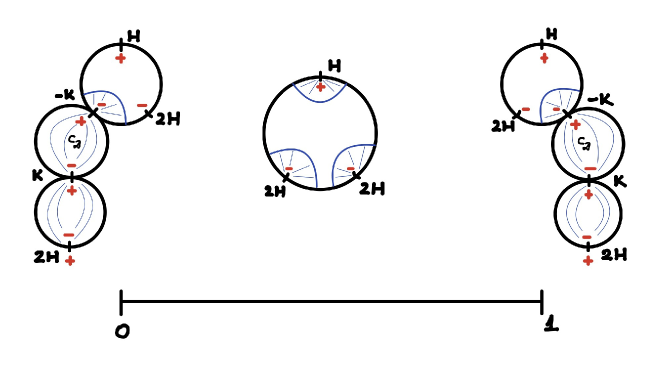
Figure 1. Definition of the coproduct on $SH_{*}(W;\mathrm{im}\,c)$.

We will now investigate conditions under which this map descends to $SH_{*}(W;\mathrm{im}\,c)$ or $\overline{SH}_{*}(W)$.

Lemma 4.1.

Assume that the dimension of the $R$-essential Weinstein domain is $2n\geq 6$. Then the chain level map ${\bm{\lambda}}_{\mathcal{D}}$ satisfies

$${\bm{\lambda}}_{\mathcal{D}}(\mathrm{im}\,c_{\mathcal{D}})\subset\mathrm{im}\,c_{\mathcal{D}}\otimes FC_{*}(2H)+FC_{*}(2H)\otimes\mathrm{im}\,c_{\mathcal{D}},$$

i.e. the pair $(\mathrm{im}\,c_{\mathcal{D}},\mathrm{im}\,c_{\mathcal{D}})$ is a coideal pair for the map ${\bm{\lambda}}_{\mathcal{D}}$.

Proof.

For action reasons ${\bm{\lambda}}_{\mathcal{D}}(\mathrm{im}\,c_{\mathcal{D}})\subset FC_{*}^{=0}(2H)\otimes FC_{*}^{=0}(2H)$, and we have natural identifications $FC_{*}^{=0}(2H)=FC_{*}(2K)\simeq FC_{*}(K)=MC^{n-*}(K)$. Note that $\bm{\lambda}_{\mathcal{D}}c_{\mathcal{D}}$ appears as a term in the boundary of an operation ${\bm{\beta}}={\bm{\beta}}_{\mathcal{D}}$ of degree $-2$ (with respect to the Conley-Zehnder grading), and the other terms in the boundary lie in $\mathrm{im}\,c_{\mathcal{D}}\otimes FC_{*}(2H)+FC_{*}(2H)\otimes\mathrm{im}\,c_{\mathcal{D}}$ (cf. [6]). See Figure 2.

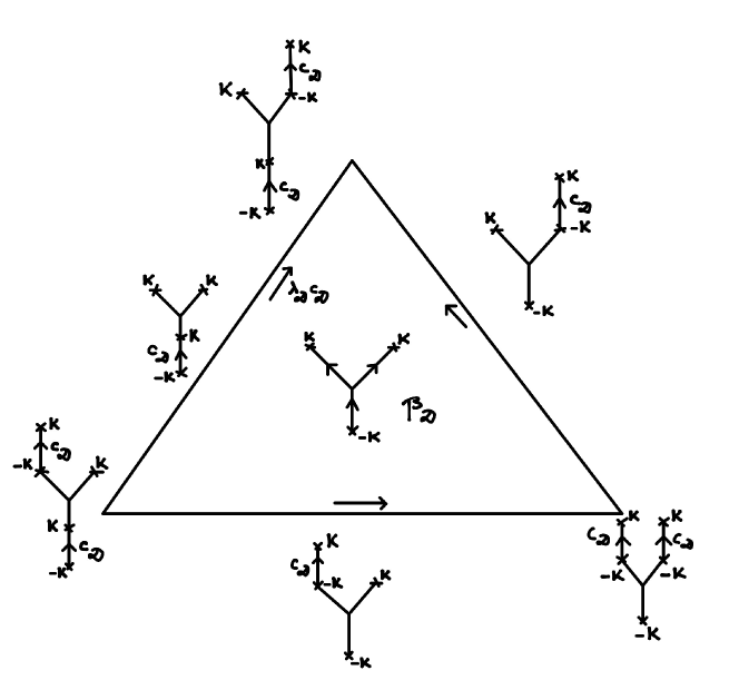
Figure 2. The operation ${\bm{\beta}}_{\mathcal{D}}$.

The operation $\bm{\beta}$ counts $2$-parameter families of cohomological $Y$-graphs with one input $x$ in $MC^{*}(-K)$ and two outputs $a,b$ in $MC^{*}(K)$. The condition for $0$-dimensional moduli spaces is $\mathrm{ind}_{K}a+\mathrm{ind}_{K}b+(2n-\mathrm{ind}_{-K}x)-4n+2=0$, which is equivalent to

$$\mathrm{ind}_{K}a+\mathrm{ind}_{K}b=-2+2n+\mathrm{ind}_{-K}x.$$

The left hand side of this equality is $\leq 2n$, while the right hand side is $\geq-2+3n$. The equality is therefore never satisfied if $n\geq 3$, which implies $\bm{\beta}=0$ and thus the lemma. ∎

Proposition 4.2.

Assume that the dimension of the $R$-essential Weinstein domain is $2n\geq 6$. A choice of $R$-essential Morse function $K$, a choice of Morse-Smale gradient-like vector field, and a choice of continuation data $\mathcal{D}$ from $-K$ to $K$, induce a degree $-n+1$ coproduct

$$\bm{\lambda}_{\mathcal{D}}:SH_{*}(W;\mathrm{im}\,c)\to SH_{*}(W;\mathrm{im}\,c)\otimes SH_{*}(W;\mathrm{im}\,c).$$

Proof.

This follows from Lemma 4.1 by passing to the limit over $R$-essential Hamiltonians which extend $K$. ∎

The dimensional assumption in the previous Proposition can be discarded if one wishes to only reduce the domain to $\overline{SH}_{*}(W)$.

Proposition 4.3.

A choice of $R$-essential Morse function $K$, a choice of Morse-Smale gradient-like vector field, and a choice of continuation data $\mathcal{D}$ from $-K$ to $K$, induce a degree $-n+1$ linear map

$$\bm{\lambda}_{\mathcal{D}}:\overline{SH}_{*}(W)\to SH_{*}(W;\mathrm{im}\,c)\otimes SH_{*}(W;\mathrm{im}\,c).$$

Proof.

Consider the chain map

$$\bm{\lambda}_{\mathcal{D}}:FC_{*}(H)\to FC_{*}(2H;\mathrm{im}\,c_{\mathcal{D}})^{\otimes 2}.$$

In the proof of Lemma 4.1 we needed to prove that this map vanishes on $\mathrm{im}\,c_{\mathcal{D}}$. We now need to prove something weaker, namely that the map $\bm{\lambda}_{\mathcal{D}\,*}$ induced in homology vanishes on $\mathrm{im}\,c_{*}$. Equivalently, it is enough to evaluate $\bm{\lambda}_{\mathcal{D}}\circ c_{\mathcal{D}}$ on an element $x\in FC_{*}(-K)$ which is a cycle and show that it is a boundary in $FC_{*}(2H;\mathrm{im}\,c_{\mathcal{D}})^{\otimes 2}$.

Denote

$$I_{\mathcal{D}}=\mathrm{im}\,c_{\mathcal{D}}\otimes FC_{*}(2H)+FC_{*}(2H)\otimes\mathrm{im}\,c_{\mathcal{D}}.$$

The analysis of the moduli space defining the operation $\bm{\beta}=\bm{\beta}_{\mathcal{D}}$ from the proof of Lemma 4.1 shows that we have

(8) $$\bm{\lambda}_{\mathcal{D}}\circ c_{\mathcal{D}}=[{\partial},\bm{\beta}_{\mathcal{D}}]\,\mbox{ mod }\,I_{\mathcal{D}}.$$

Evaluating this on a cycle $x\in FC_{*}(-K)$ we obtain

$$\bm{\lambda}_{\mathcal{D}}\circ c_{\mathcal{D}}(x) ={\partial}\bm{\beta}_{\mathcal{D}}(x)\,\mbox{ mod }\,I_{\mathcal{D}}$$

$$={\partial}\big{(}\bm{\beta}_{\mathcal{D}}(x)\,\mbox{ mod }\,I_{\mathcal{D}}\big{)},$$

which is a boundary in $FC_{*}(2H;\mathrm{im}\,c_{\mathcal{D}})^{\otimes 2}$.

In the limit over $R$-essential Hamiltonians $H$ we obtain the map

$${\bm{\lambda}}_{\mathcal{D}}:\overline{SH}_{*}(W)\to SH_{*}(W;\mathrm{im}\,c)^{\otimes 2}.$$

∎

Remark 4.4.

In the definition of $\bm{\lambda}_{\mathcal{D}}$ we used the same continuation data $\mathcal{D}$ for the continuation map $c_{\mathcal{D}}:FC_{*}(-K)\to FC_{*}(K)$ in the factorization at both ends of the $1$-parameter Floer problem. The previous results would still hold for a more general definition using different continuation data at the two ends. We will however not discuss it.

The coproducts $\bm{\lambda}_{\mathcal{D}}$ depend on the choice of $\mathcal{D}$. Next, we will explain how this dependence can be expressed in terms of secondary continuation maps.

4.2. Secondary continuation map

This map is defined via a parametrized Floer problem with parameter space $[0,1]$. For readability, we lead the discussion in two steps: we first consider a simplified setup in which the Morse function and gradient-like vector field at the endpoints are assumed to be the same, then we discuss the general case in which we allow them to be different.

In the sequel $W$ is a Weinstein domain with $R$-essential skeleton.

(1) Simplified setup: equal Morse data at the endpoints. Recall that, given an $R$-essential Morse function $K:W\to{\mathbb{R}}$ with Morse-Smale gradient-like vector field $\xi$, a choice of continuation data $\mathcal{D}$ from $(-K,-\xi)$ to $(K,\xi)$ induces a continuation map $c_{\mathcal{D}}:FC_{*}(-K)\to FC_{*}(K)$, and the map $c_{\mathcal{D}}$ does not depend on $\mathcal{D}$ (Lemma 2.3).

Definition 4.5 (secondary continuation map).

Let $\mathcal{D}_{0},\mathcal{D}_{1}$ be choices of continuation data from $(-K,-\xi)$ to $(K,\xi)$. The secondary continuation map

$$\vec{\bm{c}}_{\mathcal{D}_{0},\mathcal{D}_{1}}:FC_{*}(-K)\to FC_{*+1}(K)$$

is the degree $1$ map induced by a homotopy between $\mathcal{D}_{0}$ and $\mathcal{D}_{1}$.

The secondary continuation element, or copairing

$${\bm{c}}_{\mathcal{D}_{0},\mathcal{D}_{1}}\in\Big{(}FC_{0}(K)\otimes FC_{1}(K)\Big{)}\oplus\Big{(}FC_{1}(K)\otimes FC_{0}(K)\Big{)}$$

is defined from the secondary continuation map by viewing the input in $FC_{*}(-K)\equiv FC_{*}(K)^{\vee}$ as the first output in $FC_{*}(K)$, i.e. $\vec{\bm{c}}_{\mathcal{D}_{0},\mathcal{D}_{1}}=(\mathrm{ev}\otimes 1)(1\otimes{\bm{c}}_{\mathcal{D}_{0},\mathcal{D}_{1}})$, with $\mathrm{ev}:FC_{*}(K)^{\vee}\otimes FC_{*}(K)\to R$ the evaluation.

That the range of bi-degrees for the components of ${\bm{c}}_{\mathcal{D}_{0},\mathcal{D}_{1}}$ is restricted to $(0,1)$ and $(1,0)$ is a consequence of the fact that the Floer complex of an $R$-essential Hamiltonian is supported in degrees $0,\dots,n$.

Lemma 4.6.

(i) The secondary continuation map is a chain map which is well-defined up to chain homotopy.

(ii) The secondary continuation element is a cycle which is well-defined up to chain homotopy.

Proof.

(i) By definition $\vec{\bm{c}}_{\mathcal{D}_{0},\mathcal{D}_{1}}$ is a chain homotopy between $c_{\mathcal{D}_{0}}$ and $c_{\mathcal{D}_{1}}$. Since $c_{\mathcal{D}_{1}}=c_{\mathcal{D}_{0}}$, we infer that $\vec{\bm{c}}_{\mathcal{D}_{0},\mathcal{D}_{1}}$ is a chain map.

That the map induced by $\vec{\bm{c}}_{\mathcal{D}_{0},\mathcal{D}_{1}}$ in homology depends only on $\mathcal{D}_{0}$ and $\mathcal{D}_{1}$, and not on the choice of homotopy between the two, follows by a standard interpolation argument.

(ii) This is equivalent to (i) since the continuation element is obtained from the continuation map by dualization. ∎

Given an $R$-essential Hamiltonian $H$ with Morse truncation $K$, we consider the composition $FC_{*}(-H)\to FC_{*}(-K)\to FC_{*+1}(K)\to FC_{*+1}(H)$, where the middle map is $\vec{\bm{c}}_{\mathcal{D}_{0},\mathcal{D}_{1}}$ and the extremal maps are the projection onto the quotient complex $FC_{*}(-K)$ and the inclusion of the subcomplex $FC_{*}(K)$. We call this composition also “secondary continuation map” and denote it $\vec{\bm{c}}_{\mathcal{D}_{0},\mathcal{D}_{1}}:FC_{*}(-H)\to FC_{*+1}(H)$. After passing to homology, we obtain in the limit a map

$$\vec{\bm{c}}_{\mathcal{D}_{0},\mathcal{D}_{1}}:SH^{-*}(W)\to SH_{*+1}(W).$$

Equivalently, viewing the input as an output we obtain a degree $1$ “secondary continuation element”

$${\bm{c}}_{\mathcal{D}_{0},\mathcal{D}_{1}}\in\big{(}SH_{0}(W)\otimes SH_{1}(W)\Big{)}\oplus\Big{(}SH_{1}(W)\otimes SH_{0}(W)\Big{)}\subset SH_{*}(W)^{\otimes 2}.$$

For the next lemma we introduce the following notation. The reduced continuation element

$$\bar{\bm{c}}_{\mathcal{D}_{0},\mathcal{D}_{1}}\in SH_{*}(W;\mathrm{im}\,c)^{\otimes 2}$$

is the projection of ${\bm{c}}_{\mathcal{D}_{0},\mathcal{D}_{1}}$ under the map $SH_{*}(W)\to SH_{*}(W;\mathrm{im}\,c)$. Given a choice of continuation data $\mathcal{D}$ from $(-K,-\xi)$ to $(K,\xi)$ consisting of a homotopy $(H_{s,t},J_{s,t})$ of Hamiltonians and almost complex structures, the reverse continuation data $\mathcal{D}^{op}$ is given by the homotopy $(-H_{-s,1-t},J_{-s,1-t})$.

Recall also the coproduct ${\bm{\lambda}}_{\mathcal{D}}:SH_{*}(W)\to SH_{*}(W;\mathrm{im}\,c)^{\otimes 2}$ and the unit ${\bm{\eta}}$ for the product on $SH_{*}(W)$.

Lemma 4.7.

We have

$$\bar{\bm{c}}_{\mathcal{D}^{op},\mathcal{D}}={\bm{\lambda}}_{\mathcal{D}}{\bm{\eta}}.$$

Proof.

This follows by a gluing argument from the fact that ${\bm{\eta}}$ is given by a count of genus $0$ curves with one negative puncture. See Figure 3. ∎

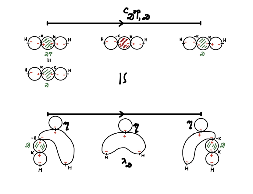
Figure 3. Secondary continuation map from coproduct.

(2) General setup: different Morse data at the endpoints. Let $(K,\xi,\mathcal{D})$ and $(K^{\prime},\xi^{\prime},\mathcal{D}^{\prime})$ be two choices of $R$-essential Morse functions, Morse-Smale gradient-like vector fields and continuation data $\mathcal{D}$ from $(-K,-\xi)$ to $(K,\xi)$ and $\mathcal{D}^{\prime}$ from $(-K^{\prime},-\xi^{\prime})$ to $(K^{\prime},\xi^{\prime})$.

In addition, we choose continuation data $\mathcal{C}$ from $(K,\xi)$ to $(K^{\prime},\xi^{\prime})$. This determines also continuation data from $(-K,-\xi)$ to $(-K^{\prime},-\xi^{\prime})$, denoted $-\mathcal{C}$. This choice of continuation data $\mathcal{C}$ is necessary, as it will reflect the dependence of the coproduct on the choice of Morse function.

Definition 4.8.

The secondary continuation map

$$\vec{\bm{c}}_{\mathcal{D},\mathcal{D}^{\prime},\mathcal{C}}:FC_{*}(-K)\to FC_{*+1}(K^{\prime})$$

is the degree $1$ map defined in three steps as follows:

(i) we form continuation data $\tilde{\mathcal{D}}=\mathcal{D}\#\mathcal{C}$ from $-K$ to $K^{\prime}$ by appending $\mathcal{C}$ to $\mathcal{D}$ at the output;

(ii) we form continuation data ${\tilde{\mathcal{D}}}^{\prime}=-\mathcal{C}\#\mathcal{D}^{\prime}$ from $-K$ to $K^{\prime}$ by appending $\mathcal{D}^{\prime}$ to $-\mathcal{C}$ at the output;

(iii) we choose a homotopy from $\tilde{\mathcal{D}}$ to ${\tilde{\mathcal{D}}}^{\prime}$ and define $\vec{\bm{c}}_{\mathcal{D},\mathcal{D}^{\prime},\mathcal{C}}=\vec{\bm{c}}_{\tilde{\mathcal{D}},{\tilde{\mathcal{D}}}^{\prime}}$ to be the induced map $FC_{*}(-K)\to FC_{*+1}(K^{\prime})$.

Definition 4.9.

The secondary continuation element, or copairing

$${\bm{c}}_{\mathcal{D},\mathcal{D}^{\prime},\mathcal{C}}\in\Big{(}FC_{0}(K)\otimes FC_{1}(K^{\prime})\Big{)}\oplus\Big{(}FC_{1}(K)\otimes FC_{0}(K^{\prime})\Big{)}$$

is defined from the secondary continuation map by viewing the input in $FC_{*}(-K)\equiv FC_{*}(K)^{\vee}$ as the first output in $FC_{*}(K)$.

The following is the analogue of Lemma 4.6.

Lemma 4.10.

(i) The secondary continuation map is a chain map which is well-defined up to chain homotopy.

(ii) The secondary continuation element is a cycle which is well-defined up to chain homotopy. ∎

Given $R$-essential Hamiltonians $H$, $H^{\prime}$ with Morse truncations $K$, $K^{\prime}$, we consider the composition

$$FC_{*}(-H)\to FC_{*}(-K)\to FC_{*+1}(K^{\prime})\to FC_{*+1}(H^{\prime}),$$

where the middle map is $\vec{\bm{c}}_{\mathcal{D},\mathcal{D}^{\prime},\mathcal{C}}$ and the extremal maps are the projection onto the quotient complex $FC_{*}(-K)$ and the inclusion of the subcomplex $FC_{*}(K^{\prime})$. We call this composition also “secondary continuation map” and denote it $\vec{\bm{c}}_{\mathcal{D},\mathcal{D}^{\prime},\mathcal{C}}:FC_{*}(-H)\to FC_{*+1}(H^{\prime})$. After passing to homology, we obtain in the limit a map

$$\vec{\bm{c}}_{\mathcal{D},\mathcal{D}^{\prime},\mathcal{C}}:SH^{-*}(W)\to SH_{*+1}(W).$$

Equivalently, viewing the input as an output we obtain a degree $1$ “secondary continuation element”

$${\bm{c}}_{\mathcal{D},\mathcal{D}^{\prime},\mathcal{C}}\in\big{(}SH_{0}(W)\otimes SH_{1}(W)\Big{)}\oplus\Big{(}SH_{1}(W)\otimes SH_{0}(W)\Big{)}\subset SH_{*}(W)^{\otimes 2}.$$

Projecting via the map $SH_{*}(W)\to SH_{*}(W;\mathrm{im}\,c)$ we get

$$\bar{\bm{c}}_{\mathcal{D},\mathcal{D}^{\prime},\mathcal{C}}\in SH_{*}(W;\mathrm{im}\,c)^{\otimes 2}.$$

4.3. Dependence of the coproduct on the choice of continuation data

Let $(K,\xi,\mathcal{D})$ and $(K^{\prime},\xi^{\prime},\mathcal{D}^{\prime})$ be two choices of $R$-essential Morse functions, Morse-Smale gradient-like vector fields and continuation data from $(-K,-\xi)$ to $(K,\xi)$ and from $(-K^{\prime},-\xi^{\prime})$ to $(K^{\prime},\xi^{\prime})$. Choose also continuation data $\mathcal{C}$ from $(K,\xi)$ to $(K^{\prime},\xi^{\prime})$, which determines also continuation data $-\mathcal{C}$ from $(-K,-\xi)$ to $(-K^{\prime},-\xi^{\prime})$.

Recall the coproducts ${\bm{\lambda}}_{\mathcal{D}},{\bm{\lambda}}_{\mathcal{D}^{\prime}}:\overline{SH}_{*}(W)\to SH_{*}(W;\mathrm{im}\,c)^{\otimes 2}$ and the notation $\mathcal{D}^{op}$. We will use the continuation elements ${\bm{c}}_{\mathcal{D},\mathcal{D}^{\prime},\mathcal{C}}$ and ${\bm{c}}_{{\mathcal{D}^{\prime}}^{op},\mathcal{D}^{op},\mathcal{C}^{op}}$ as defined in the previous subsection.

Proposition 4.11.

We have

$${\bm{\lambda}}_{\mathcal{D}^{\prime}}={\bm{\lambda}}_{\mathcal{D}}+({\bm{\mu}}\otimes 1)(1\otimes{\bm{c}}_{\mathcal{D},\mathcal{D}^{\prime},\mathcal{C}})-(1\otimes{\bm{\mu}})({\bm{c}}_{{\mathcal{D}}^{op},{\mathcal{D}^{\prime}}^{op},\mathcal{C}^{op}}\otimes 1)$$

as maps $\overline{SH}_{*}(W)\to SH_{*}(W;\mathrm{im}\,c)^{\otimes 2}$.

The terms on the right hand side have to be interpreted as follows: the multiplication involving ${\bm{\mu}}$ is performed in $\overline{SH}_{*}(W)$, and the result is further reduced to $SH_{*}(W;\mathrm{im}\,c)$.

Proof.

The proof is straightforward from the definitions and relies on the following observation: at an endpoint of the parametrizing interval for ${\bm{\lambda}}_{\mathcal{D}}$, the configuration consisting of a curve with one input, two outputs and a continuation-map-curve attached at one of the outputs can be reinterpreted as a configuration consisting of a curve with two inputs, one output, and a continuation-element-curve attached at one of the inputs. At the starting point of the parametrizing interval we read $\tau{\bm{c}}_{\mathcal{D}^{\prime},\mathcal{D},\mathcal{C}}$ and then use the equality

$$\tau{\bm{c}}_{\mathcal{D}^{\prime},\mathcal{D},\mathcal{C}}=-{\bm{c}}_{\mathcal{D}^{op},{\mathcal{D}^{\prime}}^{op},\mathcal{C}^{op}}.$$

∎

In the special case $\mathcal{D}^{\prime}=\mathcal{D}^{op}$ and with $\mathcal{C}$ the constant continuation data (which we drop from the notation) we obtain the following.

Corollary 4.12.

We have

$${\bm{\lambda}}_{\mathcal{D}^{op}}={\bm{\lambda}}_{\mathcal{D}}+({\bm{\mu}}\otimes 1)(1\otimes{\bm{c}}_{\mathcal{D},\mathcal{D}^{op}})+(1\otimes{\bm{\mu}})({\bm{c}}_{\mathcal{D},\mathcal{D}^{op}}\otimes 1)$$

as maps $\overline{SH}_{*}(W)\to SH_{*}(W;\mathrm{im}\,c)^{\otimes 2}$.

Proof.

Using ${\bm{c}}_{\mathcal{D}^{op},\mathcal{D}}=-{\bm{c}}_{\mathcal{D},\mathcal{D}^{op}}$ and Proposition 4.11 we find

$${\bm{\lambda}}_{\mathcal{D}^{op}} ={\bm{\lambda}}_{\mathcal{D}}+({\bm{\mu}}\otimes 1)(1\otimes{\bm{c}}_{\mathcal{D},\mathcal{D}^{op}})-(1\otimes{\bm{\mu}})({\bm{c}}_{\mathcal{D}^{op},\mathcal{D}}\otimes 1)$$

$$={\bm{\lambda}}_{\mathcal{D}}+({\bm{\mu}}\otimes 1)(1\otimes{\bm{c}}_{\mathcal{D},\mathcal{D}^{op}})+(1\otimes{\bm{\mu}})({\bm{c}}_{\mathcal{D},\mathcal{D}^{op}}\otimes 1).$$

∎

Corollary 4.13.

For an $R$-essential Weinstein domain $W$ such that $H^{n-1}(W;R)=0$, the coproduct ${\bm{\lambda}}_{\mathcal{D}}$ is independent of the choice of continuation data $\mathcal{D}$.

Proof.

Given another choice of continuation data $\mathcal{D}^{\prime}$, we claim that the continuation maps $\vec{\bm{c}}_{\mathcal{D},\mathcal{D}^{\prime},\mathcal{C}}$ and $\vec{\bm{c}}_{{\mathcal{D}}^{op},{\mathcal{D}^{\prime}}^{op},\mathcal{C}^{op}}$ vanish. This implies ${\bm{\lambda}}_{\mathcal{D}^{\prime}}={\bm{\lambda}}_{\mathcal{D}}$ by Proposition 4.11.

We now prove the claim. The continuation maps act as $SH^{-*}(W)\to SH_{*+1}(W)$ and factor through the energy zero part $H_{n+*}(W;R)\to H^{n-*-1}(W;R)$. Since the homology and cohomology of $W$ are supported in degrees $0,\dots,n$, these maps can only be nonzero in degrees $*=-1,0$. We are thus left to consider the two maps

$$H_{n-1}(W;R)\to H^{n}(W)\qquad\mbox{and}\qquad H_{n}(W;R)\to H^{n-1}(W;R).$$

The condition $H^{n-1}(W;R)=0$ ensures the vanishing of the second map. This condition also implies that $\mathrm{Hom}_{R}(H_{n-1}(W;R),R)$ vanishes. Indeed, this group is a surjective image of $H^{n-1}(W;R)$ by the universal coefficient theorem (this uses that $R$ is a principal ideal domain). On the other hand, by the condition of $R$-essentiality the Morse differential ${\partial}:MC_{n}(W;R)\to MC_{n-1}(W;R)$ is zero, hence $H_{n-1}(W;R)$ is free. The vanishing of $\mathrm{Hom}_{R}(H_{n-1}(W;R),R)$ is therefore equivalent to the vanishing of $H_{n-1}(W;R)$, and this ensures the vanishing of the first map. ∎

Remark 4.14.

For the cotangent bundle $W=D^{*}M$ of an $R$-orientable manifold $M$, this recovers the corresponding result from [3, §4]. Indeed, we have $H^{n-1}(W;R)\simeq H^{n-1}(M;R)\simeq H_{1}(M;R)$ by Poincaré duality.

5. Weinstein domains with strongly $R$-essential skeleton

In this section we introduce a slightly more restrictive class of Weinstein domains with $R$-essential skeleton which have the following nice features :

• the dimension condition $2n\geq 6$ from the definition of the coproducts $\bm{\lambda}=\bm{\lambda}_{\mathcal{D}}$ can be dropped.

• reduced symplectic homology and symplectic homology relative to the continuation map are equal, so that they provide a common domain of definition for the pair of pants product and for the pair of pants secondary coproducts.

Definition 5.1.

A Weinstein domain with strongly $R$-essential skeleton is a Weinstein domain with $R$-essential skeleton such that the canonical map

$$\overline{SH}_{*}(W)\to SH_{*}(W;\mathrm{im}\,c)$$

is an isomorphism.

The terminology is motivated by Proposition 3.7: given a Weinstein domain $W$ with $R$-essential skeleton, a sufficient condition which ensures that it has strongly $R$-essential skeleton is injectivity of the map $H^{n}(W;R)\to SH_{0}(W;R)$. This means that the top dimensional cells of the skeleton are homologically essential not only in the Morse (zero energy) sector, but also inside the full symplectic homology group.

Example 5.2.

Examples of Weinstein domains which have a strongly $R$-essential skeleton include the following.

(i) Disc cotangent bundles of closed orientable manifolds (in the non-orientable case they have strongly ${\mathbb{Z}}/2$-essential skeleton).

(ii) Subcritical Weinstein domains.

(iii) Weinstein domains $W$ with $R$-essential skeleton which have vanishing first Chern class and which admit a Liouville form whose closed Reeb orbits on the boundary ${\partial}W$ which are contractible in the interior $W$ have Conley-Zehnder index $\neq 0,1$ (this ensures that nonconstant orbits cannot kill any generators of $H^{n}(W)$). For example:

• plumbings of cotangent bundles of simply-connected closed manifolds of dimension $\geq 3$. Indeed, as shown in [8, Theorem 54], their boundaries admit contact forms whose closed Reeb orbits are nondegenerate and have Conley-Zehnder index $\geq 2$.

• Milnor fibers of isolated singularities which admit contact forms on the boundary as above. Specific examples are the Milnor fillings of Brieskorn manifolds $\Sigma(\ell,2,\dots,2)$ of dimension $2n-1\geq 5$. The indices have been computed explicitly by Ustilovsky [16] and van Koert [17], see also Uebele [15] and Fauck [10]. That all indices are $\geq 2$ in this case can be seen using the formula from [10, Proposition 103]. Many other Brieskorn manifolds satisfy the assumption on the indices, although it is unclear whether they can be characterized in a simple manner.

Proposition 5.3.

Let $W$ be a Weinstein domain with strongly $R$-essential skeleton. The choice of an $R$-essential Morse function $K$, of a Morse-Smale gradient-like vector field, and of continuation data $\mathcal{D}$ from $-K$ to $K$, determines a coproduct

$$\bm{\lambda}=\bm{\lambda}_{\mathcal{D}}:\overline{SH}_{*}(W)\to\overline{SH}_{*}(W)^{\otimes 2}.$$

Proof.

The map ${\bm{\lambda}}_{\mathcal{D}}:\overline{SH}_{*}(W)\to SH_{*}(W;\mathrm{im}\,c)^{\otimes 2}$ from Proposition 4.3 lifts to

$${\bm{\lambda}}_{\mathcal{D}}:\overline{SH}_{*}(W)\to\overline{SH}_{*}(W)^{\otimes 2}$$

by the strong $R$-essentiality assumption. ∎

Remark 5.4.

It is instructive to ponder the role played by strong $R$-essentiality in the previous proof, allowing to remove the dimensionality assumption $2n\geq 6$ from Proposition 4.2. In the sequel we will use strong $R$-essentiality as a standing assumption and prove robust algebraic properties of the coproduct in that setup. All the sequel results have counterparts for Weinstein domains with $R$-essential skeleton, which however require additional dimensional assumptions.

6. Bialgebra structure on reduced symplectic homology

6.1. Unital infinitesimal anti-symmetric bialgebras

Let $A$ be a graded module over a unital commutative ring $R$. We assume that $A$ is of finite type, meaning that it is free and finite dimensional in each degree. We recall from [5] the following definition.

Definition 6.1.

A unital infinitesimal anti-symmetric bialgebra is a graded module $A$ endowed with a product ${\bm{\mu}}:A\otimes A\to A$, a coproduct ${\bm{\lambda}}:A\to A\otimes A$ and an element ${\bm{\eta}}\in A$ which satisfy the following relations:

• (unit) the element ${\bm{\eta}}$ is the unit for the product ${\bm{\mu}}$.

• (associativity) the product ${\bm{\mu}}$ is associative.

• (coassociativity) the coproduct ${\bm{\lambda}}$ is coassociative.

• (unital infinitesimal relation)

  $${\bm{\lambda}}{\bm{\mu}}=(-1)^{|{\bm{\lambda}}||{\bm{\mu}}|}\Big{(}(1\otimes{\bm{\mu}})({\bm{\lambda}}\otimes 1)+({\bm{\mu}}\otimes 1)(1\otimes{\bm{\lambda}})\Big{)}-(-1)^{|{\bm{\mu}}|}({\bm{\mu}}\otimes{\bm{\mu}})(1\otimes{\bm{\lambda}}{\bm{\eta}}\otimes 1).$$

• (unital anti-symmetry)

  $$(-1)^{|{\bm{\mu}}|(|{\bm{\lambda}}|+1)}(1\otimes{\bm{\mu}})(\tau{\bm{\lambda}}\otimes 1)+(-1)^{|{\bm{\lambda}}|(|{\bm{\mu}}|+1)}({\bm{\mu}}\tau\otimes 1)(1\otimes{\bm{\lambda}})$$

  $$\hskip 142.26378pt-(-1)^{|{\bm{\lambda}}|+|{\bm{\mu}}|}({\bm{\mu}}\tau\otimes{\bm{\mu}})(1\otimes{\bm{\lambda}}{\bm{\eta}}\otimes 1)$$

  $$=(-1)^{|{\bm{\lambda}}||{\bm{\mu}}|}\tau(1\otimes{\bm{\mu}}\tau)({\bm{\lambda}}\otimes 1)-(-1)^{(|{\bm{\lambda}}|+1)(|{\bm{\mu}}|+1)}\tau({\bm{\mu}}\otimes 1)(1\otimes\tau{\bm{\lambda}})$$

  $$\hskip 142.26378pt-(-1)^{|{\bm{\mu}}|}\tau({\bm{\mu}}\otimes{\bm{\mu}}\tau)(1\otimes{\bm{\lambda}}{\bm{\eta}}\otimes 1).$$

Evaluating the (unital anti-symmetry) relation on ${\bm{\eta}}\otimes{\bm{\eta}}$ we obtain in particular

$$\tau{\bm{\lambda}}{\bm{\eta}}=(-1)^{|{\bm{\lambda}}|}{\bm{\lambda}}{\bm{\eta}}.$$

The notion of a unital infinitesimal anti-symmetric bialgebra is invariant under shift.

It is useful to give a graphical interpretation of the (unital infinitesimal relation) and of (unital anti-symmetry). Let us represent ${\bm{\mu}}$ and ${\bm{\lambda}}$ in the form of Y-shaped graphs, with the inputs depicted in clockwise order with respect to the output for ${\bm{\mu}}$, and the outputs depicted in counterclockwise order with respect to the input for ${\bm{\lambda}}$. See Figure 4.

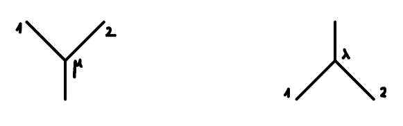
Figure 4. The product ${\bm{\mu}}$ and the coproduct ${\bm{\lambda}}$.

Then the (unital infinitesimal relation) takes the form depicted in Figure 5, and (unital anti-symmetry) takes the form depicted in Figure 6.

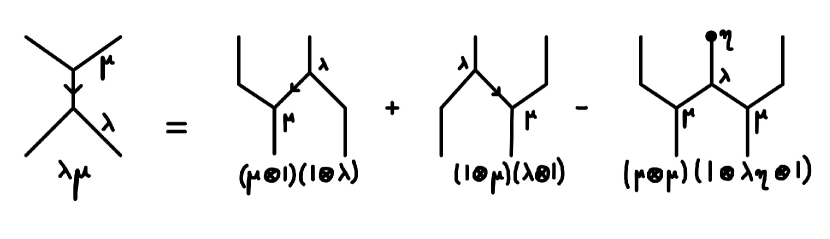
Figure 5. The unital infinitesimal relation for $|{\bm{\mu}}|=0$.

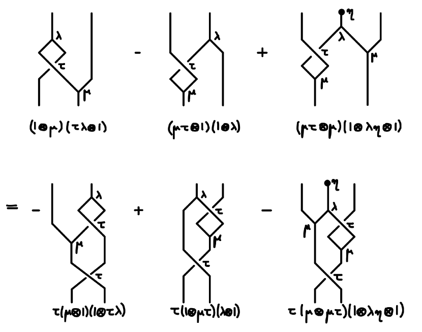
Figure 6. Unital anti-symmetry for $|{\bm{\mu}}|=0$ and $|{\bm{\lambda}}|$ odd.

Remark 6.2 (The commutative and cocommutative case).

If ${\bm{\mu}}$ is commutative and ${\bm{\lambda}}$ is cocommutative,

$${\bm{\mu}}\tau=(-1)^{|{\bm{\mu}}|}{\bm{\mu}}\quad\text{and}\quad\tau{\bm{\lambda}}=(-1)^{|{\bm{\lambda}}|}{\bm{\lambda}},$$

then (unital anti-symmetry) is a consequence of the (unital infinitesimal relation). To see this, simply observe that the unital infinitesimal relation transforms the left hand side of the unital anti-symmetry relation to $(-1)^{|{\bm{\mu}}|+|{\bm{\lambda}}|}{\bm{\lambda}}{\bm{\mu}}$ and the right hand side to $(-1)^{|{\bm{\mu}}|}\tau{\bm{\lambda}}{\bm{\mu}}$, so the two sides are equal.

Remark 6.3 (Involutivity, cf. [5]).

If $2\neq 0$ in the ring $R$, and if ${\bm{\mu}}$ and ${\bm{\lambda}}$ are commutative resp. cocommutative of opposite parity, then the following (involutivity) relation holds:

$${\bm{\mu}}{\bm{\lambda}}=0.$$

Indeed, we have

$${\bm{\mu}}{\bm{\lambda}}=(-1)^{|{\bm{\lambda}}|}{\bm{\mu}}(\tau{\bm{\lambda}})=(-1)^{|{\bm{\lambda}}|}({\bm{\mu}}\tau){\bm{\lambda}}=(-1)^{|{\bm{\lambda}}|+|{\bm{\mu}}|}{\bm{\mu}}{\bm{\lambda}}=-{\bm{\mu}}{\bm{\lambda}}.$$

6.2. Bialgebra structure on reduced homology

Let $W$ be a Weinstein domain of dimension $2n$ with strongly $R$-essential skeleton. We fix an $R$-essential Morse function $K$, a Morse-Smale gradient-like vector field for $K$, continuation data from $-K$ to $K$, and denote this entire set of data by $\mathcal{D}$. Shifted reduced homology

$$\overline{S{\mathbb{H}}}_{*}(W)=\overline{SH}_{*+n}(W)$$

carries the pair-of-pants product ${\bm{\mu}}$ of degree $0$ with unit ${\bm{\eta}}$, and it also carries the coproduct ${\bm{\lambda}}_{\mathcal{D}}$ of odd degree $1-2n$ defined above.

Theorem 6.4.

Let $W$ be a strongly $R$-essential Weinstein domain of dimension $2n\geq 4$. Shifted reduced symplectic homology

$$(\overline{S{\mathbb{H}}}_{*}(W),{\bm{\mu}},{\bm{\lambda}}_{\mathcal{D}},{\bm{\eta}})$$

is a unital infinitesimal anti-symmetric bialgebra which is commutative and cocommutative.

The proof of Theorem 6.4 is spread over the next subsections. Coassociativity of ${\bm{\lambda}}_{\mathcal{D}}$ is proved in §6.3. The unital infinitesimal relation is proved in §6.4. The unital anti-symmetry relation is proved in §6.5. Although this is implied in the closed string case by the unital infinitesimal relation in conjunction with commutativity and cocommutativity (Remark 6.2), we give a proof relying on an explicit analysis of moduli spaces which applies verbatim in the open string case, see §8

Remark 6.5.

We expect that the statement also holds in dimension $2$. The current restriction on the dimension arises from our method of proof of coassociativity.

Remark 6.6.

One can define a dual notion of reduced symplectic cohomology $\overline{SH}^{*}(W)=\ker\,{\varepsilon}_{*}$, with ${\varepsilon}_{*}$ defined in §3.1. It carries a cocommutative counital coproduct ${\bm{\mu}}^{\vee}$ dual to ${\bm{\mu}}$, a commutative product ${\bm{\lambda}}_{\mathcal{D}}^{\vee}$ dual to ${\bm{\lambda}}_{\mathcal{D}}$, and the resulting structure is that of a counital infinitesimal anti-symmetric bialgebra in the sense of [5].

6.3. Coassociativity

Proposition 6.7.

The coproduct ${\bm{\lambda}}_{\mathcal{D}}$ is coassociative if $W$ has dimension $2n\geq 4$.

Proof.

Let $H$ be an $R$-essential Hamiltonian with truncation $K$.

In Figure 7 we depict a family of Floer problems parametrized by a $3$-dimensional polytope which we call The House. The source Riemann surface for this Floer problem is a genus zero curve with four punctures constrained to lie on a circle, one positive with weight $1$, and three negative with respective weights equal to $3$. This Riemann surface degenerates to nodal curves along the boundary of the polytope as indicated in Figure 7. The House has 7 codimension 1 faces. We refer to each of the two triangles together with their adjacent quadrilaterals as The Back and Front Walls. We refer to the 2 pentagonal faces and to the hexagonal face as The Longitudinal Walls. Each of the faces of The House is labeled by a possibly nodal Riemann surface, and parametrizes a Floer problem with that nodal Riemann surface at the source. We indicate in the figure the Hamiltonians at the intermediate nodes (either $-K$, or multiples of $H$ indicated by numbers).

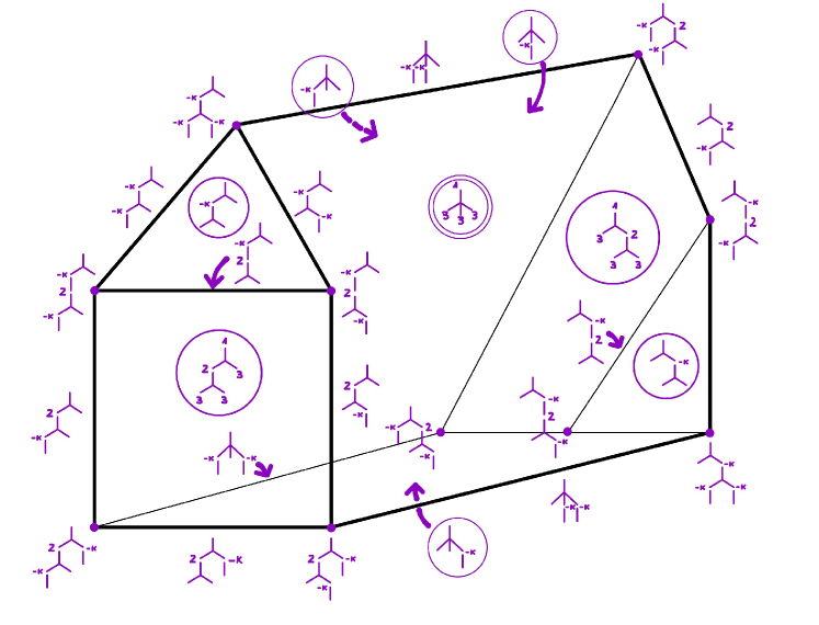
Figure 7. The House.

The Floer degeneration data is chosen such that the $0$-dimensional solutions of the Floer problems parametrized by the quadrilateral faces define the compositions $({\bm{\lambda}}_{\mathcal{D}}\otimes 1){\bm{\lambda}}_{\mathcal{D}}$ and $(1\otimes{\bm{\lambda}}_{\mathcal{D}}){\bm{\lambda}}_{\mathcal{D}}$.

Denote ${\bm{B}}_{\mathcal{D}}$ the operation with three outputs obtained by dualizing the input of the operation ${\bm{\beta}}_{\mathcal{D}}$ from the proof of Lemma 4.1. The Floer problems parametrized by the triangular faces can then be interpreted as $(1\otimes 1\otimes{\bm{\mu}})({\bm{B}}_{\mathcal{D}}\otimes 1)$ and $({\bm{\mu}}\otimes 1\otimes 1)(1\otimes{\bm{B}}_{\mathcal{D}})$.

The $0$-dimensional solutions of the Floer problems parametrized by The Longitudinal Walls define operations which, when they are applied to $FC_{*}(H)$, land in $I_{\mathcal{D}}=\mathrm{im}\,c_{\mathcal{D}}\,\otimes FC_{*}(3H)\otimes FC_{*}(3H)+FC_{*}(3H)\otimes\,\mathrm{im}\,c_{\mathcal{D}}\,\otimes FC_{*}(3H)+FC_{*}(3H)\otimes FC_{*}(3H)\otimes\,\mathrm{im}\,c_{\mathcal{D}}\,$. These operations vanish in the quotient $\left(FC_{*}(3H)/\mathrm{im}\,c_{\mathcal{D}}\right)^{\otimes 3}$.

The count of elements of $0$-dimensional moduli spaces of solutions of the Floer problem parametrized by The House defines an operation

$$\Theta:FC_{*}(H)\to FC_{*}(3H;\mathrm{im}\,c_{\mathcal{D}})^{\otimes 3}$$

such that

$$[{\partial},\Theta]=({\bm{\lambda}}_{\mathcal{D}}\otimes 1){\bm{\lambda}}_{\mathcal{D}}+(1\otimes{\bm{\lambda}}_{\mathcal{D}}){\bm{\lambda}}_{\mathcal{D}}$$

$$+(1\otimes 1\otimes{\bm{\mu}})({\bm{B}}_{\mathcal{D}}\otimes 1)-({\bm{\mu}}\otimes 1\otimes 1)(1\otimes{\bm{B}}_{\mathcal{D}}).$$

We evaluate this relation on $c_{\mathcal{D}}(x)$ with $x\in FC_{*}(-K)$ a cycle. We claim that the terms $(1\otimes 1\otimes{\bm{\mu}})({\bm{B}}_{\mathcal{D}}\otimes c_{\mathcal{D}}(x))$ and $({\bm{\mu}}\otimes 1\otimes 1)(c_{\mathcal{D}}(x)\otimes{\bm{B}}_{\mathcal{D}})$ are both boundaries in $FC_{*}(3H;\mathrm{im}\,c_{\mathcal{D}})$. Both terms are treated similarly and we focus in the sequel on $(1\otimes 1\otimes{\bm{\mu}})({\bm{B}}_{\mathcal{D}}\otimes c_{\mathcal{D}}(x))$.

We dualize the chain level relations satisfied by ${\bm{\beta}}_{\mathcal{D}}$ and ${\bm{\lambda}}_{\mathcal{D}}$ to get

$$[{\partial},{\bm{B}}_{\mathcal{D}}]=\sum_{\tiny\mathrm{cyclic}}(c_{\mathcal{D}}\otimes 1\otimes 1)\sigma_{\mathcal{D}}$$

for an element $\sigma_{\mathcal{D}}\in FC_{*}(-K)\otimes FC_{*}(K)\otimes FC_{*}(K)$ obtained by dualizing the input of the coproduct ${\bm{\lambda}}_{\mathcal{D}}$, and

$${\bm{\mu}}(1\otimes c_{\mathcal{D}})=c_{\mathcal{D}}m_{L}+[{\partial},\tau_{R}]$$

for operations $m_{L}:FC_{*}(K)\otimes FC_{*}(-K)\to FC_{*}(-K)$ obtained by dualizing ${\bm{\mu}}$ and $\tau_{R}:FC_{*}(K)\otimes FC_{*}(-K)\to FC_{*}(K)$ obtained by dualizing ${\bm{\lambda}}_{\mathcal{D}}$.

This gives

$$(1\otimes 1 \otimes{\bm{\mu}})({\bm{B}}_{\mathcal{D}}\otimes c_{\mathcal{D}}(x))$$

$$=(1\otimes 1\otimes c_{\mathcal{D}}m_{L})({\bm{B}}_{\mathcal{D}}\otimes x)+(1\otimes 1\otimes[{\partial},\tau_{R}])({\bm{B}}_{\mathcal{D}}\otimes x)$$

$$=(1\otimes 1\otimes[{\partial},\tau_{R}])({\bm{B}}_{\mathcal{D}}\otimes x)\,\mbox{ mod }\,I_{\mathcal{D}}$$

$$={\partial}(1\otimes 1\otimes\tau_{R})({\bm{B}}_{\mathcal{D}}\otimes x)+(1\otimes 1\otimes\tau_{R})({\partial}{\bm{B}}_{\mathcal{D}}\otimes x)\,\mbox{ mod }\,I_{\mathcal{D}}$$

$$=(1\otimes 1\otimes\tau_{R})({\partial}{\bm{B}}_{\mathcal{D}}\otimes x)+\,\mbox{ bdry mod }\,I_{\mathcal{D}}$$

$$=(1\otimes 1\otimes\tau_{R}(c_{\mathcal{D}}\otimes 1))(\sigma_{\mathcal{D}}\otimes x)+\,\mbox{ bdry mod }\,I_{\mathcal{D}}.$$

At this point we need conditions under which $\tau_{R}$ vanishes on $\mathrm{im}\,c_{\mathcal{D}}\otimes FC_{*}(-K)$. At zero energy the operation $\tau_{R}$ is defined by a count of gradient Y-graphs with two inputs and one output in a $1$-parametric family. We apply this operation $\tau_{R}(c_{\mathcal{D}}\otimes 1)$ to inputs $x$, $y$ which are critical points of $-K$, and obtain an output $z$ which is a critical point of $K$. The index condition is

$$\mathrm{ind}_{K}(x)+\mathrm{ind}_{K}(y)+\mathrm{ind}_{K}(z)=4n-1.$$

Given that the critical points of $K$ have index $\in\{0,\dots,n\}$, such an equality can only be satisfied if $n=1$ and all the critical points have equal index $1$. This situation has been precisely excluded by the assumptions.

To summarize, given a cycle $x\in FC_{*}(-K)$ the map $FC_{*}(H)\to FC_{*}(3H;\mathrm{im}\,c_{\mathcal{D}})^{\otimes 3}$ given by $({\bm{\lambda}}_{\mathcal{D}}\otimes 1){\bm{\lambda}}_{\mathcal{D}}+(1\otimes{\bm{\lambda}}_{\mathcal{D}}){\bm{\lambda}}_{\mathcal{D}}$ evaluates on $c_{\mathcal{D}}(x)$ into a boundary. This implies that the map induced in the limit over $H$ on $\overline{S{\mathbb{H}}}_{*}(W)$ vanishes, which proves coassociativity. ∎

6.4. The unital infinitesimal relation

Proposition 6.8.

The unital infinitesimal relation holds:

(9) $${\bm{\lambda}}_{\mathcal{D}}{\bm{\mu}}=(1\otimes{\bm{\mu}})({\bm{\lambda}}_{\mathcal{D}}\otimes 1)+({\bm{\mu}}\otimes 1)(1\otimes{\bm{\lambda}}_{\mathcal{D}})-({\bm{\mu}}\otimes{\bm{\mu}})(1\otimes{\bm{\lambda}}_{\mathcal{D}}{\bm{\eta}}\otimes 1).$$

Proof.

Let $\mathcal{M}_{0,4}^{\circ}$ be the moduli space of genus $0$ Riemann surfaces $\Sigma_{2;2}$ with 2 positive punctures and 2 negative punctures constrained to lie on a circle and ordered such that the negative punctures do not separate the positive punctures. This moduli space is diffeomorphic to an open interval and its compactification $\overline{\mathcal{M}}_{0,4}^{\circ}$ is diffeomorphic to a closed interval whose ends correspond to nodal curves with two irreducible components and matching asymptotic markers at their common node, each containing two punctures: at one end the two punctures on each irreducible component have the same sign, and at the other end they have opposite signs. We choose a family of cylindrical ends over $\overline{\mathcal{M}}_{0,4}^{\circ}$ which is compatible with splittings at the boundary.

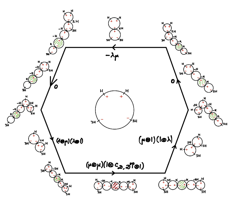
Figure 8. Proof of the unital infinitesimal relation.

We now consider an oriented $2$-dimensional hexagon $\mathcal{P}$ which is fibered over $\overline{\mathcal{M}}_{0,4}^{\circ}$ and which parametrizes Floer data $(H_{\tau},\beta_{\tau})$, $\tau\in\mathcal{P}$ as described below. The projection map $\mathcal{P}\to\overline{\mathcal{M}}_{0,4}^{\circ}$ forgets the Floer data and contracts the unstable components of the underlying Riemann surfaces. We fix an $R$-essential Hamiltonian $H$ and refer to Figure 8 for a pictorial description of the hexagon $\mathcal{P}$.

• The Riemann surface which underlies under the projection map the top horizontal side $\mathcal{P}^{\text{top}}$ of $\mathcal{P}$ is the endpoint of $\overline{\mathcal{M}}_{0,4}^{\circ}$ for which the punctures on each irreducible component have the same sign. The Floer data on the irreducible component that contains the two positive punctures is fixed and equal to $(H,\beta)$, with $\beta$ a closed $1$-form that has weights $1$ at the positive punctures and weight $2$ at the node. The Floer data on the irreducible component that contains the two negative punctures is the Floer data that defines the secondary coproduct $-\bm{\lambda}_{\mathcal{D}}$. In particular, at the endpoints of $\mathcal{P}^{\text{top}}$ the Floer data is defined on a Riemann surface with two unstable components and is non-zero on these, so that the solutions of the Floer equation are stable maps.

• The projection map $\mathcal{P}^{\text{top, vert}}\to\overline{\mathcal{M}}_{0,4}^{\circ}$ defined on each of the two top vertical sides of $\mathcal{P}$ is a smooth diffeomorphism. The underlying Riemann surface for the Floer data has one stable component with 2 positive punctures, 1 negative puncture and one node, and 2 unstable components. The second negative puncture is located on the unstable component which is not adjacent to the stable component. The Floer data on the unstable components consists of homotopies from $-H$ to $-K$, from $-K$ to $K$ given by $\mathcal{D}$, and from $K$ to $3H$. The Floer data on the stable component is $(H,\beta_{\tau})$, where $\beta_{\tau}$ interpolates within the space of closed $1$-forms with weights $(1,1;3,-1)$ (resp. $(1,1;-1,3)$), between a split $1$-form with weights $(1,1;2)$ and $(2;3,-1)$ (resp. $(2;-1,3)$), and a split $1$-form with weights $(1;2,-1)$ and $(1,2;3)$ (resp. $(1;-1,2)$ and $(2,1;3)$).

• The Riemann surface which underlies under the forgetful map the Floer data on the bottom vertical sides $\mathcal{P}^{\text{bottom,vert}}$ and on the bottom horizontal side $\mathcal{P}^{\text{bottom}}$ is the endpoint of $\overline{\mathcal{M}}_{0,4}^{\circ}$ for which the punctures on each irreducible component have different signs.

  Along the two sides $\mathcal{P}^{\text{bottom,vert}}$, the Floer data is as follows:

  • on the irreducible component for which the node is labeled as positive, the Floer data is constant equal to $(H,\beta)$, with $\beta$ a closed $1$-form that has weights $(2,1;3)$ (resp. $(1,2;3)$).

  • on the irreducible component for which the node is labeled as negative, the Floer data defines the secondary coproduct $\bm{\lambda}_{\mathcal{D}}$. In particular, at the endpoints of $\mathcal{P}^{\text{bottom,vert}}$ the underlying nodal Riemann surface has two unstable components, on which the Floer data consists of homotopies $-H\to-K\stackrel{{\scriptstyle\mathcal{D}}}{{\longrightarrow}}K\to 3H$ or $-2H\to-K\stackrel{{\scriptstyle\mathcal{D}}}{{\longrightarrow}}K\to 3H$.

  Along the bottom horizontal side $\mathcal{P}^{\text{bottom}}$ the underlying Riemann surface has two stable components with 2 punctures and 1 node each, separated by an unstable component. At the endpoints of $\mathcal{P}^{\text{bottom}}$ the unstable component is replaced by two unstable components. The Floer data is constant on the stable components along $\mathcal{P}^{\text{bottom}}$, whereas on the unstable component it is given by a family of homotopies $H_{\tau,s}$ from $-2H$ to $2H$, interpolating between the broken homotopy $-2H\to-K\stackrel{{\scriptstyle\mathcal{D}}}{{\longrightarrow}}K\to 2H$ and the broken homotopy $-2H\to-K\stackrel{{\scriptstyle\mathcal{D}^{op}}}{{\longrightarrow}}K\to 2H$. (In order to write this, one needs to reinterpret the Floer data at the endpoint of $\mathcal{P}^{\text{bottom}}$ so that it fits with the Floer data at the starting point of the following bottom vertical side.)

Given orbits $x_{0},x_{1}\in\mathcal{P}(H)$ and $y_{0},y_{1}\in\mathcal{P}(3H)$, we define the moduli space $\mathcal{M}^{\mathcal{P}}(x_{0},x_{1};y_{0},y_{1})$ consisting of pairs $(\tau,u)$, $\tau\in\mathcal{P}$, $u:\Sigma_{\tau}\to\widehat{W}$ such that

(10) $$(du-X_{H_{\tau}}\otimes\beta_{\tau})^{0,1}=0$$

and $u$ is asymptotic to $x_{0},x_{1}$, resp. $y_{0},y_{1}$ at the positive, resp. negative punctures. The anti-holomorphic part of $du-X_{H_{\tau}}\otimes\beta_{\tau}$ is considered with respect to a $\mathcal{P}$-family of compatible almost complex structures $(J_{\tau})$ which are cylindrical in the symplectization end $[1,\infty)\times{\partial}W$. For a generic such choice the moduli space $\mathcal{M}^{\mathcal{P}}(x_{0},x_{1};y_{0},y_{1})$ is a smooth manifold with boundary, of dimension

$$\dim\mathcal{M}^{\mathcal{P}}(x_{0},x_{1};y_{0},y_{1})=\mathrm{CZ}(x_{0})+\mathrm{CZ}(x_{1})-\mathrm{CZ}(y_{0})-\mathrm{CZ}(y_{1})-2n+2.$$

The signed count of elements in $0$-dimensional such moduli spaces defines a degree $-2n+2$ map

$$\Gamma:FC_{*}(H)^{\otimes 2}\to FC_{*}(3H)^{\otimes 2}.$$

The $1$-dimensional moduli spaces $\mathcal{M}^{\mathcal{P}}(x_{0},x_{1};y_{0},y_{1})$, which correspond to $\mathrm{CZ}(x_{0})+\mathrm{CZ}(x_{1})-\mathrm{CZ}(y_{0})-\mathrm{CZ}(y_{1})-2n+1=0$, are compact up to Floer breaking. By examining their oriented boundary we obtain the equation

$$[{\partial},\Gamma]=\Gamma_{{\partial}\mathcal{P}},$$

where $\Gamma_{{\partial}\mathcal{P}}:FC_{*}(H)^{\otimes 2}\to FC_{*}(3H)^{\otimes 2}$ is the degree $-2n+1$ map obtained by counting solutions of the parametrized Floer equation (10) parametrized by the oriented boundary of $\mathcal{P}$.

We now project onto $FC_{*}(3H;\mathrm{im}\,c)^{\otimes 2}$ and obtain the equation

$$\Gamma_{{\partial}\mathcal{P}}=-{\bm{\lambda}}_{\mathcal{D}}\bm{\mu}+(1\otimes\bm{\mu})({\bm{\lambda}}_{\mathcal{D}}\otimes 1)+(\bm{\mu}\otimes 1)(1\otimes{\bm{\lambda}}_{\mathcal{D}})+({\bm{\mu}}\otimes{\bm{\mu}})(1\otimes{\bm{c}}_{\mathcal{D},\mathcal{D}^{\mathrm{op}}}\otimes 1).$$

Indeed, each of the sides of $\mathcal{P}$ contributes as follows to $\Gamma_{{\partial}\mathcal{P}}$:

• The contribution of the top horizontal side of $\mathcal{P}$ is $-{\bm{\lambda}}_{\mathcal{D}}\bm{\mu}$.

• The contribution of the bottom vertical sides of $\mathcal{P}$ is $(1\otimes\bm{\mu})({\bm{\lambda}}_{\mathcal{D}}\otimes 1)+(\bm{\mu}\otimes 1)(1\otimes{\bm{\lambda}}_{\mathcal{D}})$.

• The contribution of the top vertical sides of $\mathcal{P}$ is zero in the quotient complex.

• The contribution of the bottom horizontal side of $\mathcal{P}$ is $({\bm{\mu}}\otimes{\bm{\mu}})(1\otimes{\bm{c}}_{\mathcal{D},\mathcal{D}^{\mathrm{op}}}\otimes 1)$.

This implies the equality

$$[{\partial},\Gamma]=-{\bm{\lambda}}_{\mathcal{D}}\bm{\mu}+(1\otimes\bm{\mu})({\bm{\lambda}}_{\mathcal{D}}\otimes 1)+(\bm{\mu}\otimes 1)(1\otimes{\bm{\lambda}}_{\mathcal{D}})+({\bm{\mu}}\otimes{\bm{\mu}})(1\otimes{\bm{c}}_{\mathcal{D},\mathcal{D}^{\mathrm{op}}}\otimes 1)$$

as maps $FC_{*}(H)^{\otimes 2}\to FC_{*}(3H;\mathrm{im}\,c)^{\otimes 2}$. As before this implies the relation

$${\bm{\lambda}}_{\mathcal{D}}{\bm{\mu}}=(1\otimes\bm{\mu})({\bm{\lambda}}_{\mathcal{D}}\otimes 1)+(\bm{\mu}\otimes 1)(1\otimes{\bm{\lambda}}_{\mathcal{D}})+({\bm{\mu}}\otimes{\bm{\mu}})(1\otimes{\bm{c}}_{\mathcal{D},\mathcal{D}^{\mathrm{op}}}\otimes 1)$$

as maps $\overline{F{\mathbb{H}}}_{*}(H)^{\otimes 2}\to F{\mathbb{H}}_{*}(3H;\mathrm{im}\,c)^{\otimes 2}$. By passing to the limit over $H$ we find the same relation as maps $\overline{S{\mathbb{H}}}_{*}(W)^{\otimes 2}\to S{\mathbb{H}}_{*}(W;\mathrm{im}\,c)^{\otimes 2}$, and further as maps $\overline{S{\mathbb{H}}}_{*}(W)^{\otimes 2}\to\overline{S{\mathbb{H}}}_{*}(W)^{\otimes 2}$ in view of strong $R$-essentiality. We conclude using that

$${\bm{c}}_{\mathcal{D},\mathcal{D}^{\mathrm{op}}}=-{\bm{c}}_{\mathcal{D}^{\mathrm{op}},\mathcal{D}}=-{\bm{\lambda}}_{\mathcal{D}}{\bm{\eta}},$$

where the first equality is a direct consequence of the definition and the second equality is the content of Lemma 4.7. ∎

6.5. The unital anti-symmetry relation

Proposition 6.9.

The unital anti-symmetry relation holds:

$$(1\otimes{\bm{\mu}})(\tau{\bm{\lambda}}_{\mathcal{D}}\otimes 1)-({\bm{\mu}}\tau\otimes 1)(1\otimes{\bm{\lambda}}_{\mathcal{D}})$$

$$\hskip 142.26378pt+({\bm{\mu}}\tau\otimes{\bm{\mu}})(1\otimes{\bm{\lambda}}_{\mathcal{D}}{\bm{\eta}}\otimes 1)$$

$$=\tau(1\otimes{\bm{\mu}}\tau)({\bm{\lambda}}_{\mathcal{D}}\otimes 1)-\tau({\bm{\mu}}\otimes 1)(1\otimes\tau{\bm{\lambda}}_{\mathcal{D}})$$

$$\hskip 142.26378pt-\tau({\bm{\mu}}\otimes{\bm{\mu}}\tau)(1\otimes{\bm{\lambda}}_{\mathcal{D}}{\bm{\eta}}\otimes 1).$$

Proof of Proposition 6.9.

The proof resembles that of Proposition 6.8. The relevant moduli space $\mathcal{M}$ is that of genus 0 Riemann surfaces with 2 positive punctures and 2 negative punctures, constrained to lie on a circle and ordered now such that the negative punctures and the positive punctures alternate. This moduli space is diffeomorphic to an open interval and its compactification $\overline{\mathcal{M}}$ is diffeomorphic to a closed interval whose ends correspond to nodal curves with two irreducible components and matching asymptotic markers at their common node, each containing 2 punctures, one negative and one positive. We choose a family of cylindrical ends over $\overline{\mathcal{M}}$ which is compatible with splittings at the boundary. We denote $\leavevmode\hbox to14.18pt{\vbox to14.18pt{\text{[drawing]}}},\leavevmode\hbox to14.18pt{\vbox to14.18pt{\text{[drawing]}}}$ the positive punctures (inputs) and $1,2$ the negative punctures (outputs).

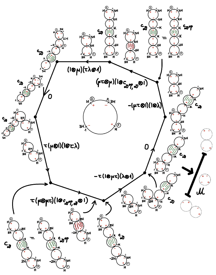
Figure 9. Proof of (unital anti-symmetry).

We further consider an oriented octogon $\mathcal{P}$ which parametrizes Floer data $(H_{\tau},\beta_{\tau})$, $\tau\in\mathcal{P}$ on suitable nodal Riemann surfaces and which is fibered over $\overline{\mathcal{M}}$ by the map which forgets the Floer data and contracts the unstable components of the underlying Riemann surfaces. The fibers of the projection $\mathcal{P}\to\overline{\mathcal{M}}$ are described as follows (Figure 9):

• The three sides above the ones marked “0” project onto the endpoint of $\overline{\mathcal{M}}$ for which the two irreducible components contain the punctures $\leavevmode\hbox to14.18pt{\vbox to14.18pt{\text{[drawing]}}},2$ and respectively $\leavevmode\hbox to14.18pt{\vbox to14.18pt{\text{[drawing]}}},1$.

• The union of the interiors of $\mathcal{P}$ and of the sides marked “0” is fibered over $\mathcal{M}$ with closed interval fibers.

• The three sides below the ones marked “0” project onto the endpoint of $\overline{\mathcal{M}}$ for which the two irreducible components contain the punctures $1,\leavevmode\hbox to14.18pt{\vbox to14.18pt{\text{[drawing]}}}$ and respectively $2,\leavevmode\hbox to14.18pt{\vbox to14.18pt{\text{[drawing]}}}$.

The underlying Riemann surfaces for the points $\tau\in\mathcal{P}$ are depicted in Figure 9: in the interior of $\mathcal{P}$ these are simply elements of $\mathcal{M}$. On the boundary of $\mathcal{P}$ these are nodal genus 0 Riemann surfaces with punctures and matching cylindrical ends at the punctures, and which may possibly have unstable components. These unstable components carry nontrivial Floer data and are stable if interpreted as Riemann surfaces with Floer data.

The Floer data $(H_{\tau},\beta_{\tau})$, $\tau\in\mathcal{P}$ consists of a constant (in $\tau$) $R$-essential Hamiltonian $H_{\tau}=H$ and of $1$-forms $\beta_{\tau}$, $\tau\in\mathcal{P}$ which satisfy $d\beta_{\tau}\leq 0$ and which have weights at the punctures as indicated in bold in Figure 9. E.g., on the top horizontal side of $\mathcal{P}$, on the irreducible component which contains the punctures $\leavevmode\hbox to14.18pt{\vbox to14.18pt{\text{[drawing]}}},2$ the weight is 1 at the positive puncture, 3 at the negative puncture, and 2 at the node. This field of $1$-forms is chosen to be compatible with splittings of Riemann surfaces over $\mathcal{P}$. Moreover, each node is directed, meaning that it is labeled as a positive puncture (input) for one of the irreducible components which contain it, and as a negative puncture (output) for the other component.

From this point on, the proof goes exactly as for Proposition 6.8. The count of elements in $0$-dimensional moduli spaces of solutions to the Floer problem parametrized by $\mathcal{P}$ defines a map $\Gamma:FC_{*}(H)^{\otimes 2}\to FC_{*}(3H;\mathrm{im}\,c_{\mathcal{D}})^{\otimes 2}$ of degree $-2n+2$. The count of elements in $0$-dimensional moduli spaces of solutions to the Floer problem parametrized by the oriented boundary of $\mathcal{P}$ defines a map $\Gamma_{{\partial}\mathcal{P}}$ of degree $-2n+1$ with the same source and target, such that

$$[{\partial},\Gamma]=\Gamma_{{\partial}\mathcal{P}}.$$

Inspection of the boundary shows that, upon quotienting the target by $\mathrm{im}\,c_{\mathcal{D}}$, we have

$$\Gamma_{{\partial}\mathcal{P}}= (1\otimes{\bm{\mu}})(\tau{\bm{\lambda}}_{\mathcal{D}}\otimes 1)-({\bm{\mu}}\tau\otimes 1)(1\otimes{\bm{\lambda}}_{\mathcal{D}})$$

$$\hskip 142.26378pt+({\bm{\mu}}\tau\otimes{\bm{\mu}})(1\otimes{\bm{c}}_{\mathcal{D}^{op},\mathcal{D}}\otimes 1)$$

$$-\tau(1\otimes{\bm{\mu}}\tau)({\bm{\lambda}}_{\mathcal{D}}\otimes 1)+\tau({\bm{\mu}}\otimes 1)(1\otimes\tau{\bm{\lambda}}_{\mathcal{D}})$$

$$\hskip 142.26378pt+\tau({\bm{\mu}}\otimes{\bm{\mu}}\tau)(1\otimes{\bm{c}}_{\mathcal{D}^{op},\mathcal{D}}\otimes 1).$$

As in the previous proofs this implies the relation

$$(1\otimes{\bm{\mu}})(\tau{\bm{\lambda}}_{\mathcal{D}}\otimes 1)-({\bm{\mu}}\tau\otimes 1)(1\otimes{\bm{\lambda}}_{\mathcal{D}})$$

$$\hskip 142.26378pt+({\bm{\mu}}\tau\otimes{\bm{\mu}})(1\otimes{\bm{c}}_{\mathcal{D}^{op},\mathcal{D}}\otimes 1)$$

$$=\tau(1\otimes{\bm{\mu}}\tau)({\bm{\lambda}}_{\mathcal{D}}\otimes 1)-\tau({\bm{\mu}}\otimes 1)(1\otimes\tau{\bm{\lambda}}_{\mathcal{D}})$$

$$\hskip 142.26378pt-\tau({\bm{\mu}}\otimes{\bm{\mu}}\tau)(1\otimes{\bm{c}}_{\mathcal{D}^{op},\mathcal{D}}\otimes 1)$$

as maps $\overline{F{\mathbb{H}}}_{*}(H)^{\otimes 2}\to F{\mathbb{H}}_{*}(3H;\mathrm{im}\,c)^{\otimes 2}$. By passing to the limit over $H$ we find the same relation as maps $\overline{S{\mathbb{H}}}_{*}(W)^{\otimes 2}\to S{\mathbb{H}}_{*}(W;\mathrm{im}\,c)^{\otimes 2}$, and further as maps $\overline{S{\mathbb{H}}}_{*}(W)^{\otimes 2}\to\overline{S{\mathbb{H}}}_{*}(W)^{\otimes 2}$ in view of strong $R$-essentiality. We conclude using that ${\bm{c}}_{\mathcal{D}^{\mathrm{op}},\mathcal{D}}={\bm{\lambda}}_{\mathcal{D}}{\bm{\eta}}$ (Lemma 4.7). ∎

6.6. Cocommutativity

Graded commutativity of the product $\bm{\mu}$ is standard. We address cocommutativity of the coproduct $\bm{\lambda}_{\mathcal{D}}$.

Proposition 6.10.

The coproduct ${\bm{\lambda}}_{\mathcal{D}}$ is cocommutative on $\overline{S{\mathbb{H}}}_{*}({\partial}W)$, meaning that

$${\bm{\lambda}}_{\mathcal{D}}+\tau{\bm{\lambda}}_{\mathcal{D}}=0.$$

Proof.

Let $H$ be an $R$-essential Hamiltonian and let $\mathcal{D}$ be continuation data. We set up a Floer problem parametrized by the square $[0,1]\times[0,1]$ as follows (see Figure 10). The underlying Riemann surface is a genus 0 curve with 3 punctures, 1 positive and 2 negative, together with cylindrical ends which depend on $(\sigma,\tau)\in[0,1]\times[0,1]$. The cylindrical end at the positive puncture is fixed with respect to some given parametrization of the Riemann surface, and this uniquely identifies its complement with the disc $D^{2}$. The two negative punctures are fixed along each of the vertical sides, and they move along a half-Dehn twist as we traverse the square along segments $[0,1]\times\{\tau\}$. Thus the two negative punctures get exchanged as we move from one vertical side to the other. One important point in the construction is that the negative punctures are ordered, i.e. labeled by $1$ and $2$. When traversing from the left vertical side to the right vertical side, this labeling is switched. We also choose cylindrical ends at the negative punctures over $[0,1]\times[0,1]$ in such a way that over the two vertical sides the cylindrical ends are switched from one puncture to the other.

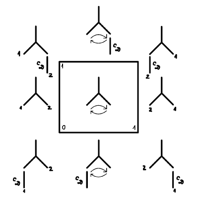
Figure 10. Cocommutativity of ${\bm{\lambda}}_{\mathcal{D}}$.

On the first vertical side the Floer data corresponds to the one defining the coproduct ${\bm{\lambda}}_{\mathcal{D}}$. On the second vertical side the Floer data corresponds to the one defining the composition $-\tau{\bm{\lambda}}_{\mathcal{D}}$ between the tensor product twist and the coproduct.

Denoting $\Gamma,\Gamma_{\partial}:FC_{*}(H)\to FC_{*}(2H)\otimes FC_{*}(2H)$ the operations defined by the count of the elements of 0-dimensional moduli spaces of the Floer problem parametrized by $[0,1]\times[0,1]$, respectively by ${\partial}([0,1]\times[0,1])$, we obtain a relation

$$[{\partial},\Gamma]=\Gamma_{\partial}.$$

We then have

$$\Gamma_{\partial}=-\tau{\bm{\lambda}}_{\mathcal{D}}-{\bm{\lambda}}_{\mathcal{D}}$$

as maps $FC_{*}(H)\to FC_{*}(2H;\mathrm{im}\,c_{\mathcal{D}})^{\otimes 2}$, because the operations that are read along the two horizontal sides have image contained inside $\mathrm{im}\,c_{\mathcal{D}}\otimes FC_{*}(2H)+FC_{*}(2H)\otimes\mathrm{im}\,c_{\mathcal{D}}$. Passing to homology and in the limit over $H$ we obtain the equality ${\bm{\lambda}}_{\mathcal{D}}+\tau{\bm{\lambda}}_{\mathcal{D}}=0$ as maps $\overline{S{\mathbb{H}}}_{*}(W)\to S{\mathbb{H}}_{*}(W;\mathrm{im}\,c_{\mathcal{D}})^{\otimes 2}$. The conclusion follows by $R$-essentiality. ∎

7. Splittings of Rabinowitz Floer homology

The goal of this section is to exhibit splittings of the Rabinowitz Floer homology group which involve reduced homology and cohomology and are compatible with the product and coproduct.

In §7.1 we recall from [6] the cone description of the product and coproduct on Rabinowitz Floer homology of a Liouville domain. In §7.2 we give an invariant definition of Rabinowitz Floer homology as a colimit in groupoids, which allows us to understand the various identifications involved in the proof of invariance for the cone description. In §7.3 we discuss the properties of the long exact sequence of the pair $(V,{\partial}V)$ for a Liouville domain $V$ from the perspective of product and coproduct structures. In §7.4 we specialize to strongly $R$-essential Weinstein domains and show that this long exact sequence, rephrased as a short exact sequence in terms of reduced homology, admits non-canonical splittings. In §7.5 we discuss the failure of canonicity of the splitting maps. We conclude with §7.6 where we show how the unital infinitesimal relation in reduced homology is implied by associativity of the product on the cone.

7.1. Cone description of Rabinowitz Floer homology

Let $V$ be a Liouville domain of dimension $2n$ and denote $S{\mathbb{H}}_{*}({\partial}V)=SH_{*+n}({\partial}V)$ the shifted Rabinowitz Floer homology of ${\partial}V$. We proved in [4] that this is a biunital coFrobenius bialgebra with degree $0$ product ${\bm{\mu}}$ and degree $1-2n$ coproduct ${\bm{\lambda}}$.

It was observed in [7] that Rabinowitz Floer homology can be alternatively described as a cone, and Venkatesh [18] went a step further by adopting the cone perspective as definition. This proved effective in contexts where action filtration arguments were not readily available.

In [6] we described the product structure on Rabinowitz Floer homology from the cone perspective. Dualizing that construction yields a description of the coproduct, and we now summarize the two.

Let $H$ be a Hamiltonian which is admissible for symplectic homology and denote $\mathcal{A}=FC_{*+n}(H)$, $\mathcal{M}=\mathcal{A}^{\vee}[2n]=FC_{*+n}(-H)$, $\mathcal{A}^{\prime}=FC_{*+n}(2H)$, $\mathcal{M}^{\prime}=\mathcal{A}^{\prime\vee}[2n]=FC_{*+n}(-2H)$. Given a choice of continuation data $\mathcal{D}$ from (a Morse truncation of) $-H$ to $H$, we denote

$$c=c_{\mathcal{D}}:\mathcal{M}\to\mathcal{A}$$

the corresponding continuation map, and we use the same notation for the continuation maps $\mathcal{M}\to\mathcal{A}^{\prime}$, $\mathcal{M}^{\prime}\to\mathcal{A}$, and $\mathcal{M}^{\prime}\to\mathcal{A}^{\prime}$. Note that $c^{\vee}$ is canonically identified with $c_{\mathcal{D}^{op}}$, the continuation map determined by the reverse continuation data $\mathcal{D}^{op}$.

Product on the cone. In [6] we constructed maps $\mu:\mathcal{A}\otimes\mathcal{A}\to\mathcal{A}^{\prime}$ (product), $m_{R}:\mathcal{M}^{\prime}\otimes\mathcal{A}\to\mathcal{M}$ and $m_{L}:\mathcal{A}\otimes\mathcal{M}^{\prime}\to\mathcal{M}$ (module structure) obtained by dualizing $\mu$ at the output and at one of the two inputs, $\sigma:\mathcal{M}^{\prime}\otimes\mathcal{M}^{\prime}\to\mathcal{M}$ (secondary product), $\tau_{L}:\mathcal{M}^{\prime}\otimes\mathcal{A}\to\mathcal{A}^{\prime}$ and $\tau_{R}:\mathcal{A}\otimes\mathcal{M}^{\prime}\to\mathcal{A}^{\prime}$ (secondary module structure), and finally $\beta:\mathcal{M}^{\prime}\otimes\mathcal{M}^{\prime}\to\mathcal{A}^{\prime}$. We showed in [6] that, up to considering suitable action windows, these maps fit together into a linear map

$${\bm{\mu}}_{Cone}:Cone(c)\otimes Cone(c)\to Cone(c)$$

which induces in homology and in the limit a product ${\bm{\mu}}_{Cone}$ isomorphic to the product ${\bm{\mu}}$ on $S{\mathbb{H}}_{*}({\partial}V)$. These maps are an action truncated version of the notion of $A_{2}$-structure studied in [6].

Coproduct on the cone. The above maps can be dualized in order to obtain a cone description of the coproduct on Rabinowitz Floer homology. More precisely, we consider the following: the map $\sigma^{\vee}:\mathcal{A}\to\mathcal{A}^{\prime}\otimes\mathcal{A}^{\prime}$; the maps $\tau_{L}^{\vee}:\mathcal{M}^{\prime}\to\mathcal{M}\otimes\mathcal{A}^{\prime}$ and $\tau_{R}^{\vee}:\mathcal{M}^{\prime}\to\mathcal{A}^{\prime}\otimes\mathcal{M}$; the map $\mu^{\vee}:\mathcal{M}^{\prime}\to\mathcal{M}\otimes\mathcal{M}$; the maps $m_{L}^{\vee}:\mathcal{A}\to\mathcal{A}^{\prime}\otimes\mathcal{M}$ and $m_{R}^{\vee}:\mathcal{A}\to\mathcal{M}\otimes\mathcal{A}^{\prime}$; and finally $\beta^{\vee}:\mathcal{M}^{\prime}\to\mathcal{A}^{\prime}\otimes\mathcal{A}^{\prime}$. Arguments dual to those of [6] show that, up to considering suitable action windows, these maps fit together into a linear map

$${\bm{\lambda}}_{Cone}:Cone(c^{\vee})\to Cone(c^{\vee})\otimes Cone(c^{\vee}).$$

This family of maps induces in homology and in the limit a coproduct ${\bm{\lambda}}_{Cone}$ isomorphic to the coproduct ${\bm{\lambda}}$ on $S{\mathbb{H}}_{*}({\partial}V)$.

Remark 7.1.

For action reasons the image of the map $\beta$ is contained in the 0-energy sector $FC_{*}^{=0}(2H)$. In case $V$ is an $R$-essential Weinstein domain of dimension $2n\geq 6$, the maps $\beta$ and $\beta^{\vee}$ vanish identically. See the proof of Lemma 4.1.

Secondary continuation map and $A_{2}^{+}$-structures. That the product ${\bm{\mu}}_{Cone}$ and the coproduct ${\bm{\lambda}}_{Cone}$ involve $Cone(c)$, respectively $Cone(c^{\vee})$, has interesting implications. In order to construct a product and a coproduct on the same cone, one needs to interpolate between the continuation data $\mathcal{D}$ and $\mathcal{D}^{op}$. Denote

$$\vec{\bm{c}}=\vec{\bm{c}}_{\mathcal{D},\mathcal{D}^{op}}:\mathcal{M}\to\mathcal{A}[1]$$

the secondary continuation map determined by such an interpolation from $\mathcal{D}$ to $\mathcal{D}^{op}$. By definition we have

$$c^{\vee}-c=[{\partial},\vec{\bm{c}}\,].$$

We will use in the sequel the same notation for the secondary continuation maps $\mathcal{M}\to\mathcal{A}[1]$, $\mathcal{M}^{\prime}\to\mathcal{A}[1]$, and $\mathcal{M}^{\prime}\to\mathcal{A}^{\prime}[1]$.

The isomorphism between $Cone(c)$ and $Cone(c^{\vee})$ can be nontrivial, precisely to the extent to which the secondary continuation map is nontrivial. We explain this in the following section, and we give here an equivalent perspective on the matter using the formalism of $A_{2}^{+}$-structures studied in [6, §7]. This formalism consists in recovering the previous maps from the following smaller set of operations. Given the continuation data $\mathcal{D}$ we define the following maps:

$$c_{0}\in\mathcal{A}\otimes\mathcal{A}.$$

This is the bivector dual to the continuation map $c$. Note that $\tau c_{0}$ is then the bivector dual to the continuation map $c^{\vee}$.

$$Q_{0}\in\mathcal{A}\otimes\mathcal{A}.$$

This is the bivector dual to the secondary continuation map $\vec{\bm{c}}$ and satisfies $\tau c_{0}-c_{0}=[{\partial},Q_{0}]$.

$$\mu:\mathcal{A}\otimes\mathcal{A}\to\mathcal{A}^{\prime}$$

of degree $0$. This is the usual pair of pants product in Floer theory.

$$\lambda:\mathcal{A}\to\mathcal{A}^{\prime}\otimes\mathcal{A}^{\prime}$$

of degree $1-2n$. This is defined from a parametrized Floer problem for pairs of pants with parameter space the 1-simplex by splitting off the continuation map $c=c_{\mathcal{D}}$ at the negative punctures at the boundary of the simplex.

$$B:R\to\mathcal{A}^{\prime}\otimes\mathcal{A}^{\prime}\otimes\mathcal{A}^{\prime}$$

of degree $2-4n$ and cyclically symmetric. This is defined from a parametrized Floer problem for pairs of pants with parameter space the 2-simplex by splitting off the continuation map $c=c_{\mathcal{D}}$ at the negative punctures at the boundary of the simplex.

This data determines operations $m_{L}$, $m_{R}$, $\sigma$, $\tau_{L}$, $\tau_{R}$, $\beta$ as in [6, §7.2]. The key idea is that, upon dualizing $\mu$, $\lambda$ or $B$ at some of their inputs or outputs, one needs to further interpolate between the continuation map $c^{\vee}$ arising from the dualization and the continuation map $c$ involved in the cone. This interpolation makes use of the secondary continuation bivector $Q_{0}$. The outcome is a product ${\bm{\mu}}_{\mathcal{D}}$ on $Cone(c)$.

A similar procedure can be carried over in order to define 1-to-2 operations $\sigma^{\vee}$, $\tau_{L}^{\vee}$, $\tau_{R}^{\vee}$, $\mu^{\vee}$, $m_{L}^{\vee}$, $m_{R}^{\vee}$, $\beta^{\vee}$ as above, which assemble into a coproduct ${\bm{\lambda}}_{\mathcal{D}}$ on the same domain $Cone(c)$.

7.2. Rabinowitz Floer homology as a colimit in groupoids

While the chain level components of the cone product and coproduct depend a priori on the choice of continuation data determining the continuation map $c$, the induced maps in homology do not depend on these choices. We now explain this invariance property.

Recall that a set of continuation data $\mathcal{D}$ consists of a Morse function $K$ on $V$ and a homotopy $-K\to K$. This determines a continuation map $c_{\mathcal{D}}:FC_{*}(-K)\to FC_{*}(K)$. We further choose a coherent set of Hamiltonian homotopies $K\to H_{b}$ and $H_{-b}\to-K$, where $H_{b}$, $b>0$ is an admissible Hamiltonian of slope $b$ extending $K$ and $H_{-b}=-H_{b}$. We define the cone Rabinowitz Floer homology group for the continuation datum $\mathcal{D}$ to be

$$S{\mathbb{H}}_{*,\mathcal{D}}({\partial}V)=\lim\limits_{\stackrel{{\scriptstyle\longrightarrow}}{{b\to\infty}}}\lim\limits_{\stackrel{{\scriptstyle\longleftarrow}}{{a\to-\infty}}}H_{*}(Cone(c_{\mathcal{D}}:FC_{*+n}(H_{a})\to FC_{*+n}(H_{b}))),$$

where we denote $c_{\mathcal{D}}:FC_{*}(H_{a})\to FC_{*}(H_{b})$ the continuation map determined by the concatenation of the Hamiltonian homotopies $H_{a}\to-K\to K\to H_{b}$. This group carries a product ${\bm{\mu}}_{\mathcal{D}}$ and a coproduct ${\bm{\lambda}}_{\mathcal{D}}$ as explained above. We omit from the notation the data of the Hamiltonian homotopies $H_{a}\to-K$ and $K\to H_{b}$ since the resulting structures do not depend on these at homology level.

Any two continuation data $\mathcal{D}$, $\mathcal{D}^{\prime}$ can be connected by a homotopy, and such a homotopy induces a transition isomorphism

$$\Phi_{\mathcal{D},\mathcal{D}^{\prime}}:S{\mathbb{H}}_{*,\mathcal{D}}({\partial}V)\stackrel{{\scriptstyle\simeq}}{{\longrightarrow}}S{\mathbb{H}}_{*,\mathcal{D}^{\prime}}({\partial}V)$$

which intertwines the products

$$\Phi_{\mathcal{D},\mathcal{D}^{\prime}}{\bm{\mu}}_{\mathcal{D}}={\bm{\mu}}_{\mathcal{D}^{\prime}}(\Phi_{\mathcal{D},\mathcal{D}^{\prime}}\otimes\Phi_{\mathcal{D},\mathcal{D}^{\prime}})$$

and the coproducts

$$\bm{\lambda}_{\mathcal{D}^{\prime}}\Phi_{\mathcal{D},\mathcal{D}^{\prime}}=(\Phi_{\mathcal{D},\mathcal{D}^{\prime}}\otimes\Phi_{\mathcal{D},\mathcal{D}^{\prime}})\bm{\lambda}_{\mathcal{D}}.$$

The isomorphism $\Phi_{\mathcal{D},\mathcal{D}^{\prime}}$ is independent of the choice of homotopy from $\mathcal{D}$ to $\mathcal{D}^{\prime}$, and it satisfies the cocycle conditions $\Phi_{\mathcal{D}^{\prime},\mathcal{D}^{\prime\prime}}\circ\Phi_{\mathcal{D},\mathcal{D}^{\prime}}=\Phi_{\mathcal{D},\mathcal{D}^{\prime\prime}}$ and $\Phi_{\mathcal{D},\mathcal{D}}=\mathrm{Id}$. In other words, the collection of objects

$$\{S{\mathbb{H}}_{*,\mathcal{D}}({\partial}V)\}_{\mathcal{D}},$$

together with the collection of isomorphisms

$$\{\Phi_{\mathcal{D},\mathcal{D}^{\prime}}\}_{\mathcal{D},\mathcal{D}^{\prime}}$$

forms a groupoid. We define the cone Rabinowitz-Floer homology as the colimit of this groupoid,

$$S{\mathbb{H}}_{*}^{cone}({\partial}V)=\mathrm{colim}\,_{\mathcal{D}}\,S{\mathbb{H}}_{*,\mathcal{D}}({\partial}V).$$

In very explicit terms $S{\mathbb{H}}_{*}^{cone}({\partial}V)$ can be described as the quotient of the direct sum $\oplus_{\mathcal{D}}S{\mathbb{H}}_{*,\mathcal{D}}({\partial}V)$ by the submodule generated by the relations $a_{\mathcal{D}}-\Phi_{\mathcal{D},\mathcal{D}^{\prime}}a_{\mathcal{D}}$ for all $\mathcal{D},\mathcal{D}^{\prime}$ and $a_{\mathcal{D}}\in S{\mathbb{H}}_{*,\mathcal{D}}({\partial}V)$. See also [14]. The colimit inherits a canonical product

$${\bm{\mu}}:S{\mathbb{H}}_{*}^{cone}({\partial}V)\otimes S{\mathbb{H}}_{*}^{cone}({\partial}V)\to S{\mathbb{H}}_{*}^{cone}({\partial}V)$$

and coproduct

$$\bm{\lambda}:S{\mathbb{H}}_{*}^{cone}({\partial}V)\to S{\mathbb{H}}_{*}^{cone}({\partial}V)\otimes S{\mathbb{H}}_{*}^{cone}({\partial}V).$$

The canonical maps $S{\mathbb{H}}_{*,\mathcal{D}}({\partial}V)\to S{\mathbb{H}}_{*}^{cone}({\partial}V)$ fit into commutative diagrams

We proved in [6] that we have a canonical isomorphism

$$S{\mathbb{H}}_{*}^{cone}({\partial}V)\stackrel{{\scriptstyle\cong}}{{\longrightarrow}}S{\mathbb{H}}_{*}({\partial}V),$$

and this further gives rise to the diagram

Now the point is that, even in cases where different choices of continuation data $\mathcal{D}$ and $\mathcal{D}^{\prime}$ define equal chain level continuation maps $c_{\mathcal{D}}=c_{\mathcal{D}^{\prime}}$ and hence equal homology groups $S{\mathbb{H}}_{*,\mathcal{D}}({\partial}V)=S{\mathbb{H}}_{*,\mathcal{D}^{\prime}}({\partial}V)$, the transition isomorphism $\Phi_{\mathcal{D},\mathcal{D}^{\prime}}$ may be nontrivial. To see this explicitly, let $W$ be an $R$-essential Weinstein domain and $K$ a fixed $R$-essential Morse function. We proved in Lemma 2.3 that, given continuation data $\mathcal{D}$, $\mathcal{D}^{\prime}$ with Morse function $K$, the continuation maps $c_{\mathcal{D}}$ and $c_{\mathcal{D}^{\prime}}$ are equal. A choice of homotopy between $\mathcal{D}$ and $\mathcal{D}^{\prime}$ determines a degree $1$ secondary continuation map $\vec{\bm{c}}_{\mathcal{D},\mathcal{D}^{\prime}}:FC_{*}(-K)\to FC_{*+1}(K)$, well-defined up to chain homotopy. We choose the homotopies $K\to H_{b}$ for $b>0$ such that the resulting map $FC_{*}(K)\to FC_{*}(H_{b})$ is an inclusion. The isomorphism $\Phi_{\mathcal{D},\mathcal{D}^{\prime}}$ is then induced at chain level by the matrix

$$\begin{pmatrix}1&\vec{\bm{c}}_{\mathcal{D},\mathcal{D}^{\prime}}\\ 0&1\end{pmatrix}$$

with respect to the splitting $Cone(c_{\mathcal{D}})=FC_{*}(H_{b})\oplus FC_{*-1}(-H_{b})$. If the map $\vec{\bm{c}}_{\mathcal{D},\mathcal{D}^{\prime}}$ is nontrivial in homology when restricted to $\ker c$, then the isomorphism $\Phi_{\mathcal{D},\mathcal{D}^{\prime}}$ is also nontrivial.

Example 7.2.

The previous phenomenon concretely occurs already for $W=T^{*}S^{1}$. Given a perfect Morse function on $S^{1}$, extend it to a Morse function $K$ on $T^{*}S^{1}={\mathbb{R}}\times S^{1}$ by adding a positive quadratic function in the ${\mathbb{R}}$-variable, so that $K$ has a single minimum and a single critical point of index $1$. Choose continuation data in the form of a small nowhere vanishing $1$-form $\eta$ on $S^{1}$, extended to ${\mathbb{R}}\times S^{1}$ as a vector field $\hat{\eta}$ which is constant along the ${\mathbb{R}}$-coordinate. We know that the resulting continuation map $c_{\hat{\eta}}$ is zero because the Euler characteristic of $S^{1}$ is zero. We can see this explicitly as follows. Denote $\varphi_{\hat{\eta}}$ the time one flow of $\hat{\eta}$. The map $c_{\hat{\eta}}:MC^{*}(-K)\to MC^{*}(K)$ counts pairs $(\gamma_{1},\gamma_{2})$ with $\gamma_{1,2}:[0,\infty)\to T^{*}S^{1}$, $\dot{\gamma}_{1,2}=\nabla K(\gamma_{1,2})$, $\gamma_{1,2}(+\infty)\in\mathrm{Crit}(K)$, and $\gamma_{1}(0)=\varphi_{\hat{\eta}}^{-1}(\gamma_{2}(0))$. By our choice of function $K$ we necessarily have $\gamma_{1,2}(0)\in S^{1}$, so that $\gamma_{1}(0)$ and $\gamma_{2}(0)$ must be equal and coincide with a zero of $\hat{\eta}$. Since $\hat{\eta}$ has no zeroes (which reflects the vanishing of the Euler characteristic of $S^{1}$), we conclude that $c_{\hat{\eta}}$ is zero.

Consider now the continuation maps induced by $\hat{\eta}$ and $-\hat{\eta}$. While they both vanish, an interpolation between $\hat{\eta}$ and $-\hat{\eta}$ determines a chain map $\vec{\bm{c}}:MC^{*}(-K)\to MC^{*-1}(K)$ which acts nontrivially in homology. More precisely, if we denote $p,q$ the two critical points of $K$, which are also critical points of $-K$, an explicit computation shows that the map $\vec{\bm{c}}$ sends $p$ to $\pm q$ and $q$ to $\pm p$. The induced automorphism

$$\begin{pmatrix}1&\vec{\bm{c}}\\ 0&1\end{pmatrix}$$

of $Cone(c_{\hat{\eta}})=Cone(c_{-\hat{\eta}})$ is therefore nontrivial in homology.

7.3. The long exact sequence of the pair $(V,{\partial}V)$

We have already used in the definition of reduced homology the following long exact sequence of the pair $(V,{\partial}V)$ from [7]:

Our next result is a refinement of this long exact sequence to take into account products and coproducts.

Proposition 7.3.

Let $V$ be a Liouville domain. There exists a commuting diagram with exact row

(11)

in which

• the maps $\iota$ and $i$ intertwine the products $\mu$, $\bm{\mu}$ and $\lambda^{\vee}$;

• the maps $p$ and $\pi$ intertwine the coproducts $\lambda$, $\bm{\lambda}$ and $\mu^{\vee}$.

Dualizing the diagram, replacing degree $*$ by $1-2n-*$ and applying Poincaré duality $S{\mathbb{H}}_{*}({\partial}V)\cong S{\mathbb{H}}^{1-2n-*}({\partial}V)$ reproduces the same diagram reflected at its center.

Proof.

We use the cone description of Rabinowitz Floer homology and its product structures given in the previous section.

The long exact sequence of the pair is an instance of homology exact sequence of a cone, with $\iota$ induced by the inclusions $\mathcal{A}\hookrightarrow Cone(c)$ and $\pi$ induced by the projections $Cone(c)\to\mathcal{M}[-1]$. Thus $\iota$ intertwines the products $\mu$ and ${\bm{\mu}}$, whereas $\pi$ intertwines the coproducts ${\bm{\lambda}}$ and $\mu^{\vee}$.

Denote $\mathcal{A}^{=0}$ the 0-energy subcomplex of $\mathcal{A}$, and $\mathcal{A}^{>0}=\mathcal{A}/\mathcal{A}^{=0}$. The map $\lambda:\mathcal{A}\to\mathcal{A}^{\prime}\otimes\mathcal{A}^{\prime}$ is a chain map modulo $\mathrm{im}\,c$ and, because $\mathrm{im}\,c\subset\mathcal{A}^{=0}$, it induces a coproduct $\lambda$ on $S{\mathbb{H}}_{*}^{>0}(V)$. The map $p$ is induced in the limit by the composition of projections $Cone(c)\to\mathcal{A}/\mathrm{im}\,c\to\mathcal{A}^{>0}$, and it follows from the description of the coproduct on the cone that $p$ intertwines the coproducts ${\bm{\lambda}}$ and $\lambda$.

Similarly, denote $\mathcal{M}^{<0}$ the negative energy subcomplex of $\mathcal{M}$, which corresponds under algebraic duality to the positive energy subcomplex defining $SH^{*}_{>0}(V)$. The map $c^{\vee}$ vanishes on $\mathcal{M}^{<0}$ and therefore $\lambda^{\vee}:\mathcal{M}^{\prime}\otimes\mathcal{M}^{\prime}\to\mathcal{M}$ defines a chain map $\mathcal{M}^{\prime,<0}\otimes\mathcal{M}^{\prime,<0}\to\mathcal{M}^{<0}$ which induces a product $\lambda^{\vee}$ on $S{\mathbb{H}}^{*}_{>0}(V)$. The map $i$ is induced by the composition of inclusions $\mathcal{M}^{<0}\to\ker c^{\vee}\to Cone(c^{\vee})$, and it follows from the description of the product on the cone that $i$ intertwines the products.

The final claim is a consequence of the proof of Poincaré duality for cones from [6]. ∎

Remark 7.4.

(a) In Proposition 7.3 we have $pi=0$ because the map $pi$ factors as the composition

$$S{\mathbb{H}}^{1-2n-*}_{>0}(V)\cong S{\mathbb{H}}_{*}^{<0}({\partial}V)\to S{\mathbb{H}}_{*}({\partial}V)\to S{\mathbb{H}}_{*}^{\geq 0}({\partial}V)\to S{\mathbb{H}}_{*}^{>0}(V)$$

where the three terms in the middle are part of the action truncation exact sequence of ${\partial}V$. However, we do not necessarily have $\mathrm{im}\,p=\ker i$.

(b) The maps $\iota$, $\pi$, $p$ satisfy the announced properties for a presentation of Rabinowitz Floer homology as $Cone(c)$ for some given continuation map, whereas the map $i$ is seen to intertwine the product using a presentation of Rabinowitz Floer homology as $Cone(c^{\vee})$. Should one want to use the presentation of Rabinowitz Floer homology as $Cone(c)$, one would need to compose the map $i$ by an automorphism involving the secondary continuation map. This is reminiscent of the fact that the splittings discussed in the next section are not canonical.

The next Corollary is straightforward. For the statement, recall that reduced homology is $\overline{S{\mathbb{H}}}_{*}(V)=\mathrm{coker}\,{\varepsilon}$ and carries an induced product $\bar{\mu}$, whereas reduced cohomology is $\overline{SH}^{*}(V)=\ker{\varepsilon}$ and carries an induced coproduct ${\bar{\mu}}^{\vee}$.

Corollary 7.5.

Let $V$ be a Liouville domain. There exists a commuting diagram with short exact row

(12)

in which

• the maps $\iota$ and $i$ intertwine the products $\bar{\mu}$, $\bm{\mu}$ and $\lambda^{\vee}$;

• the maps $p$ and $\pi$ intertwine the coproducts $\lambda$, $\bm{\lambda}$ and ${\bar{\mu}}^{\vee}$.

Dualizing the diagram, replacing degree $*$ by $1-2n-*$ and applying Poincaré duality $S{\mathbb{H}}_{*}({\partial}V)\cong S{\mathbb{H}}^{1-2n-*}({\partial}V)$ reproduces the same diagram reflected at its center. ∎

7.4. Splittings

The results of the previous section were valid for arbitrary Liouville domains. In this section we specialize to strongly $R$-essential Weinstein domains, in which case we show that the short exact sequence from Corollary 7.5 is split, albeit not canonically.

Proposition 7.6.

Let $W$ be a strongly $R$-essential Weinstein domain of dimension $2n\geq 6$. The short exact sequence (12) admits a non-canonical splitting

(13)

via maps $\bar{p},\bar{i}$ satisfying the following conditions:

• $\bar{p}\iota=1$, $\pi\bar{i}=1$, $\bar{i}\bar{j}=i$, and $\bar{q}\bar{p}=p$.

• $\mathrm{im}\,\bar{i}=\ker\bar{p}$.

• $\bar{i}$ is a ring map with respect to the product ${\bar{\lambda}}^{\vee}=\pi{\bm{\mu}}(\bar{i}\otimes\bar{i})$ on $\overline{S{\mathbb{H}}}^{*}(W)$.

• $\bar{p}$ intertwines the coproduct on $S{\mathbb{H}}_{*}({\partial}W)$ with the coproduct $\bar{\lambda}=(\bar{p}\otimes\bar{p})\bm{\lambda}\iota$ on $\overline{S{\mathbb{H}}}_{*}(W)$.

Note that, if $\bar{i}$ is a ring map with respect to some product on $\overline{S{\mathbb{H}}}^{*}(W)$, that product is necessarily given by the formula $\pi{\bm{\mu}}(\bar{i}\otimes\bar{i})$. So this assertion is equivalent to $\mathrm{im}\,\bar{i}$ being a subalgebra. A similar observation pertains to the map $\bar{p}$.

Proof.

We will describe in detail only the splitting $\bar{p}$, the discussion of $\bar{i}$ being analogous. We fix continuation data $\mathcal{D}$.

We expand the left half of the diagram (13) as follows

The arrows labeled “coalg.” are coalgebra maps, and those labeled “alg.” are algebra maps. All the groups except $S{\mathbb{H}}_{*}(W;\mathrm{im}\,c)$ are defined for arbitrary Liouville domains. The group $S{\mathbb{H}}_{*}(W;\mathrm{im}\,c)$ is defined for Weinstein domains with $R$-essential skeleton, and the map $\overline{S{\mathbb{H}}}_{*}(W)\to S{\mathbb{H}}_{*}(W;\mathrm{im}\,c)$ is an isomorphism under the assumption of strong $R$-essentiality. The coproduct $\lambda_{\mathcal{D}}$ depends a priori on the choice of continuation data $\mathcal{D}$, see §4.3. We will now describe the map $P_{\mathcal{D}}$, and we define $\bar{p}$ to be the composition of the maps $S{\mathbb{H}}_{*}({\partial}W)\to S{\mathbb{H}}_{*}^{\geq 0}({\partial}W)\to S{\mathbb{H}}_{*}(W;\mathrm{im}\,c)\stackrel{{\scriptstyle\simeq}}{{\longleftarrow}}\overline{S{\mathbb{H}}}_{*}(W)$, as in the diagram.

As part of the continuation data $\mathcal{D}$ we have an $R$-essential Morse function $K$, and a homotopy from $-K$ to $K$ which determines a continuation map $c_{\mathcal{D}}:FC_{*}(-K)\to FC_{*}(K)$. Denote $H_{b}$ an $R$-essential Hamiltonian of non-critical slope $b>0$ which extends $K$, and denote still by $c_{\mathcal{D}}$ the continuation map $FC_{*}(-K)\to FC_{*}(H_{b})$. The group $S{\mathbb{H}}_{*}^{\geq 0}({\partial}W)$ admits a cone description as

$$SH_{*}^{\geq 0}({\partial}W)=\lim\limits_{\stackrel{{\scriptstyle\longrightarrow}}{{b\to\infty}}}H_{*}(Cone(c_{\mathcal{D}}:FC_{*}(-K)\to FC_{*}(H_{b}))).$$

Recall also that

$$SH_{*}(W;\mathrm{im}\,c)=\lim\limits_{\stackrel{{\scriptstyle\longrightarrow}}{{b\to\infty}}}H_{*}(FC_{*}(H_{b})/\mathrm{im}\,c_{\mathcal{D}}).$$

The projection from the homotopy cokernel to the cokernel

is a chain map, and it acts by $(a,\bar{x})\mapsto a\ \mathrm{mod}\ \mathrm{im}\,c_{\mathcal{D}}$. It induces in the limit $b\to\infty$ the map $P_{\mathcal{D}}:SH_{*}^{\geq 0}({\partial}W)\to SH_{*}(W;\mathrm{im}\,c)$.

We now prove that $P_{\mathcal{D}}$ is a coalgebra map. Fix a Hamiltonian $H=H_{b}$ as in the definition of the map $P_{\mathcal{D},b}$, which we denote for simplicity $P_{\mathcal{D}}$. Denote $[\bm{\lambda}]:FC_{*}(H)/\mathrm{im}\,c_{\mathcal{D}}\to FC_{*}(2H)/\mathrm{im}\,c_{\mathcal{D}}\otimes FC_{*}(2H)/\mathrm{im}\,c_{\mathcal{D}}$ the reduction of $\bm{\lambda}$ modulo the coideal pair $(\mathrm{im}\,c_{\mathcal{D}},\mathrm{im}\,c_{\mathcal{D}})$ (Lemma 4.1). Using the definition of $P_{\mathcal{D}}$ and the vanishing of the operation $\beta$ involved in the cone description of the coproduct for dimensions $2n\geq 6$, we obtain for $a\in FC_{*}(H)$ and $\bar{x}\in FC_{*-1}(-K)$:

$$(P_{\mathcal{D}}\otimes P_{\mathcal{D}})\bm{\lambda}_{Cone} (a,\bar{x})$$

$$=(P_{\mathcal{D}}\otimes P_{\mathcal{D}})\bm{\lambda}(a)+(P_{\mathcal{D}}\otimes P_{\mathcal{D}})\beta(\bar{x})$$

$$=(P_{\mathcal{D}}\otimes P_{\mathcal{D}})\bm{\lambda}(a)$$

$$=\bm{\lambda}(a)\ \mathrm{mod}\ \mathrm{im}\,c_{\mathcal{D}}\otimes FC_{*}(2H)+FC_{*}(2H)\otimes\mathrm{im}\,c_{\mathcal{D}}$$

$$=[\bm{\lambda}](a\ \mathrm{mod}\ \mathrm{im}\,c_{\mathcal{D}})$$

$$=[\bm{\lambda}]P_{\mathcal{D}}(a,\bar{x}).$$

By passing to the limit over $b\to\infty$ we obtain

$$(P_{\mathcal{D}}\otimes P_{\mathcal{D}})\circ\bm{\lambda}_{Cone}=[\bm{\lambda}_{\mathcal{D}}]\circ P_{\mathcal{D}}$$

where $\bm{\lambda}_{Cone}$ is the cone coproduct on $SH_{*}^{\geq 0}(W)$ and $[\bm{\lambda}_{\mathcal{D}}]$ is the coproduct on $SH_{*}(W;\mathrm{im}\,c)$ determined by the continuation data $\mathcal{D}$.

The relations $\bar{q}\bar{p}=p$ and $\bar{p}\iota=\mathrm{Id}$ are immediate from the definition.

We finally prove the equality $\mathrm{im}\,\bar{i}=\ker\bar{p}$. We start from the relations $\bar{p}[(a,x)]=[a\ \mathrm{mod}\ \mathrm{im}\,c]$ and $\bar{i}[x]=[(0,x)]$. Then clearly $\bar{p}\bar{i}=0$, so that $\mathrm{im}\,\bar{i}\subset\ker\bar{p}$. To prove equality, consider an element $[(a,x)]\in\ker\bar{p}$. This is represented by a cycle $(a,x)$ such that $a$ is a boundary mod $\mathrm{im}\,c$, or equivalently $(a,0)$ is a boundary. Thus $(a,x)$ is homologous to $(0,x)$ and $(0,x)$ is therefore a cycle. Hence $x\in\ker c$ and $[(a,x)]\in\mathrm{im}\,\bar{i}$. ∎

We discuss the non-canonicity of the splittings in the next subsection.

7.5. Dependence of the splittings on choices

We continue with the strongly $R$-essential Weinstein domain $W$ of dimension $2n\geq 6$ from the previous subsection. The map

$$P_{\mathcal{D}}:SH_{*}^{\geq 0}({\partial}W)\to SH_{*}(W;\mathrm{im}\,c)$$

depends on the choice of continuation data $\mathcal{D}$ through the intermediate secondary continuation maps. To see this, fix an $R$-essential Morse function $K$, denote $\mathcal{A}_{*}=FC_{*+n}(K)$ and $\mathcal{M}_{*}=FC_{*+n}(-K)$, choose continuation data $\mathcal{D}$, $\mathcal{D}^{\prime}$ for $K$ and let $\vec{\bm{c}}_{\mathcal{D},\mathcal{D}^{\prime}}:FC_{*}(-K)\to FC_{*+1}(K)$ be the chain map determined by a homotopy between $\mathcal{D}$ and $\mathcal{D}^{\prime}$. Although $c_{\mathcal{D}}=c_{\mathcal{D}^{\prime}}$, the following diagram in which the diagonal arrows are projections does not commute in general

Equivalently, the two maps

obtained by inverting the diagonal isomorphisms in the diagram below, are in general different.

The map $P_{\mathcal{D}}$, and hence the splitting from Proposition 7.6, fails to be canonical precisely to the extent to which $\lambda_{\mathcal{D}}$ also fails to be canonical. This is coherent with the fact that each map $P_{\mathcal{D}}$ is a coalgebra map for the corresponding coproduct $\lambda_{\mathcal{D}}$ on $SH_{*}(W;\mathrm{im}\,c)$. The previous discussion shows that the dependence on choices is governed by the secondary continuation maps, and in view of Corollary 4.13 and its proof we obtain

Proposition 7.7.

Let $W$ be a strongly $R$-essential Weinstein domain of dimension $2n\geq 6$. The splitting from Proposition 7.6 is canonical whenever $H^{n-1}(W;R)=0$. ∎

On the other hand, the splitting and the coproduct can be seen to be non-canonical in situations where $H^{n-1}(W;R)$ does not vanish. This already happens for $W=T^{*}S^{1}$, cf. Example 7.2 and the explicit computations of splittings from [4]. Although $T^{*}S^{1}$ does not satisfy the dimension condition $2n\geq 6$, similar computations can be carried out in higher dimensional tori.

7.6. The unital infinitesimal relation from associativity

We show in this subsection how the unital infinitesimal relation in reduced symplectic homology is implied by the associativity of the product on the cone. We use an $A_{2}$-structure determined by an $A_{2}^{+}$-structure as in §7.1, with product $\mu$ and coproduct $\lambda$. We work with a strongly $R$-essential Weinstein domain $W$ of dimension $2n\geq 6$.

Proposition 7.6 associates to any choice of continuation data $\mathcal{D}$ a splitting

(14) $$S{\mathbb{H}}_{*}({\partial}W)=\overline{S{\mathbb{H}}}_{*}(W)\oplus\overline{S{\mathbb{H}}}^{1-2n-*}(W),$$

where the product ${\bm{\mu}}$ on $S{\mathbb{H}}_{*}({\partial}W)$ restricts to the product $\mu$ on the subring $\overline{S{\mathbb{H}}}_{*}(W)$, and to the cohomology product on the subring (not containing the unit) $\overline{S{\mathbb{H}}}^{1-2n-*}(W)$. More generally, let us denote the components of the product ${\bm{\mu}}$ with respect to the splitting by

$$m^{+-}_{+}:\overline{S{\mathbb{H}}}_{*}(W)\otimes\overline{S{\mathbb{H}}}^{1-2n-*}(W)\to\overline{S{\mathbb{H}}}_{*}(W)$$

etc, where the upper indices denote the inputs, the lower index the output, $+$ corresponds to $\overline{S{\mathbb{H}}}_{*}(W)$, and $-$ to $\overline{S{\mathbb{H}}}^{1-2n-*}(W)$. Each of these maps has degree $0$.

The following result expresses the product on $S{\mathbb{H}}_{*}({\partial}W)$ in terms of $\mu$, $\lambda$, and the continuation bivector ${\bm{c}}={\bm{c}}_{\mathcal{D},\mathcal{D}^{op}}$. In the statement we use the following notation: given $\bar{f}\in\overline{S{\mathbb{H}}}^{1-2n-*}(W)$, we denote $f$ the same element with degree shifted down by $1$, i.e. $|f|=|\bar{f}|-1$.

Theorem 7.8.

Let $W$ be a strongly $R$-essential Weinstein domain of dimension $2n\geq 6$. The components of the product ${\bm{\mu}}$ on $S{\mathbb{H}}_{*}({\partial}W)$ with respect to the splitting (14) are, for $a\in\overline{S{\mathbb{H}}}_{*}(W)$ and $\bar{f},\bar{g}\in\overline{S{\mathbb{H}}}^{1-2n-*}(W)$, given by

1. $m^{++}_{+}=\mu$;

2. $\langle m^{--}_{-}(\bar{f}\otimes\bar{g}),a\rangle\\ =(-1)^{|g|+|g||f|+1}\langle g\otimes f,\lambda(a)+(-1)^{|a|}(\mu\otimes 1)(a\otimes{\bm{c}})+(1\otimes\mu)({\bm{c}}\otimes a)\rangle$;

3. $m^{++}_{-}=0$ and $m^{--}_{+}=0$;

4. $m^{-+}_{+}(\bar{f},a)=(-1)^{|f|+1}\langle f\otimes 1,\lambda(a)+(1\otimes\mu)({\bm{c}}\otimes a)\rangle$, and
   $m^{+-}_{+}(b,\bar{f})=(-1)^{|b|}\langle\lambda(b)+(-1)^{|b|}(\mu\otimes 1)(b\otimes{\bm{c}}),1\otimes f\rangle$;

5. $\langle m^{-+}_{-}(\bar{f},a),b\rangle=\langle f,\mu(a,b)\rangle$, and
   $\langle a,m^{+-}_{-}(b,\bar{f})\rangle=(-1)^{|b|}\langle\mu(a,b),f\rangle$.

Proof.

These computations rely on results from [6], and we first recall some relevant notions. The splitting of $S{\mathbb{H}}_{*}({\partial}W)$ arises from its description in terms of the cone of the continuation map $c=c_{\mathcal{D}}:\mathcal{A}^{\vee}[2n]=FC_{*+n}(-H)\to\mathcal{A}=FC_{*+n}(H)$, cf. §7.1 and §7.4. The product is determined by operations $\mu$, $m_{L}$, $m_{R}$, $\sigma$, $\tau_{R}$, $\tau_{L}$ as detailed in §7.1 (under our assumptions the operation $\beta$ vanishes). These operations are determined by the $A_{2}^{+}$-structure, consisting of the product $\mu$, the coproduct $\lambda=\lambda_{\mathcal{D}}$, and the secondary continuation bivector ${\bm{c}}={\bm{c}}_{\mathcal{D},\mathcal{D}^{op}}$, according to the formulas in [6, §7.2]. More precisely

$$\langle a,m_{L}(b,f)\rangle =\langle\mu(a,b),f\rangle,$$

$$\langle m_{R}(f,a),b\rangle =\langle f,\mu(a,b)\rangle,$$

$$\langle\sigma(f,g),a\rangle =(-1)^{(|f|+1)(|g|+1)}\langle g\otimes f,\lambda_{\mathcal{D}^{op}}(a)\rangle$$

$$=(-1)^{(|f|+1)(|g|+1)}$$

$$\qquad\quad\langle g\otimes f,\bigl{(}\lambda+(\mu\otimes 1)(1\otimes{\bm{c}})+(1\otimes\mu)({\bm{c}}\otimes 1)\bigr{)}(a)\rangle,$$

$$\tau_{R}(b,f) =\langle\lambda_{\mathcal{D},\mathcal{D}^{op}}(b),1\otimes f\rangle$$

$$=\langle\bigl{(}\lambda+(\mu\otimes 1)(1\otimes{\bm{c}})\bigr{)}(b),1\otimes f\rangle$$

$$\tau_{L}(f,a) =(-1)^{|f|+1}\langle f\otimes 1,\lambda_{\mathcal{D}^{op},\mathcal{D}}(a)\rangle$$

$$=(-1)^{|f|+1}\langle f\otimes 1,\bigl{(}\lambda+(1\otimes\mu)({\bm{c}}\otimes 1)\bigr{)}(a)\rangle.$$

Additional signs arise from the fact that one of the factors of the cone is shifted. More precisely, following [6, §2.3] we define shifted operations ${\underline{m}}_{L}$, ${\underline{m}}_{R}$, ${\underline{\tau}}_{R}$, ${\underline{\tau}}_{L}$, ${\underline{\sigma}}$ by the relations

$$m_{L}={\underline{m}}_{L}[0,1;1],\qquad m_{R}={\underline{m}}_{R}[1,0;1],$$

$$\tau_{R}={\underline{\tau}}_{R}[0,1;0],\qquad\tau_{L}={\underline{\tau}}_{L}[1,0;0],$$

$$\sigma={\underline{\sigma}}[1,1;1].$$

Here $[i,j;k]$ indicates a shift by $i$ on the first component of the source, a shift by $j$ on the second component of the source, and a shift by $k$ in the target, see [6, Appendix A]. We then have $m^{++}_{+}=\mu$, $m^{+-}_{-}={\underline{m}}_{L}$, $m^{-+}_{-}={\underline{m}}_{R}$, $m^{--}_{-}={\underline{\sigma}}$, $m^{+-}_{+}={\underline{\tau}}_{R}$, $m^{-+}_{+}={\underline{\tau}}_{L}$. Denoting $\bar{f}$, $\bar{g}$ the shifts of elements $f$, $g$, we find

$$\langle a,m^{+-}_{-}(b\otimes\bar{f})\rangle =\langle a,{\underline{m}}_{L}(b,\bar{f})\rangle=(-1)^{|b|}\langle a,m_{L}(b,f)\rangle,$$

$$\langle m^{-+}_{-}(\bar{f}\otimes a),b\rangle =\langle{\underline{m}}_{R}(\bar{f}\otimes a),b\rangle=\langle m_{R}(f,a),b\rangle,$$

$$\langle m^{--}_{-}(\bar{f}\otimes\bar{g}),a\rangle =\langle{\underline{\sigma}}(\bar{f}\otimes\bar{g}),a\rangle=(-1)^{|f|}\langle\sigma(f\otimes g),a\rangle,$$

$$m^{+-}_{+}(b\otimes\bar{f}) ={\underline{\tau}}_{R}(b\otimes\bar{f})=(-1)^{|b|}\tau_{R}(b,f),$$

$$m^{-+}_{+}(\bar{f}\otimes a) ={\underline{\tau}}_{L}(\bar{f}\otimes a)=\tau_{L}(f,a).$$

Combining these formulas with the ones for $m_{L}$, $m_{R}$, $\sigma$, $\tau_{L}$, $\tau_{R}$ yields the conclusion. ∎

Remark 7.9.

The product ${\bm{\mu}}$ on $S{\mathbb{H}}_{*}({\partial}W)$ is graded commutative, i.e. ${\bm{\mu}}={\bm{\mu}}\circ\tau$. From this perspective, the two formulas in Theorem 7.8(4) are equivalent to each other as a consequence of $m^{-+}_{+}=m^{+-}_{+}\circ\tau$, and so are the two formulas in Theorem 7.8(5) as a consequence of $m^{-+}_{-}=m^{+-}_{-}\circ\tau$.

Proposition 7.10.

The unital infinitesimal relation

$$\bar{\bm{\lambda}}\bar{\bm{\mu}}=(1\otimes\bar{\bm{\mu}})(\bar{\bm{\lambda}}\otimes 1)+(\bar{\bm{\mu}}\otimes 1)(1\otimes\bar{\bm{\lambda}})-(\bar{\bm{\mu}}\otimes\bar{\bm{\mu}})(1\otimes\bar{\bm{\lambda}}\bar{\bm{\eta}}\otimes 1)$$

on $\overline{S{\mathbb{H}}}_{*}(W)$ is implied by the associativity of ${\bm{\mu}}$ on $S{\mathbb{H}}_{*}({\partial}W)$.

Proof.

We examine the ${}^{++-}_{+}$ component of the associativity relation ${\bm{\mu}}(1\otimes{\bm{\mu}}-{\bm{\mu}}\otimes 1)=0$, which reads

$$0=m^{++}_{+}(1\otimes m^{+-}_{+})+m^{+-}_{+}(1\otimes m^{+-}_{-})-m^{+-}_{+}(m^{++}_{+}\otimes 1)-m^{--}_{+}(m^{++}_{-}\otimes 1),$$

where the first and the third summands correspond to splitting along $\overline{S{\mathbb{H}}}_{*}(W)$, and the second and the fourth summands to splitting along $\overline{S{\mathbb{H}}}^{1-2n-*}(W)$. By Theorem 7.8(3) the last summand vanishes. Now we evaluate each term on inputs $a,b\in\overline{S{\mathbb{H}}}_{*}(W)$ and $\bar{f}\in\overline{S{\mathbb{H}}}^{1-2n-*}(W)$.

Using Theorem 7.8(1) and (4) the first term becomes

$$m^{++}_{+}(1\otimes m^{+-}_{+}) (a\otimes b\otimes\bar{f})=\mu(a\otimes m^{+-}_{+}(b\otimes\bar{f}))$$

$$=\mu(a\otimes\langle\lambda(b)(-1)^{|b|}+(\mu\otimes 1)(b\otimes{\bm{c}}),1\otimes f\rangle)$$

$$=(-1)^{|b|+|a|}\langle(\mu\otimes 1)(1\otimes\lambda)(a\otimes b),1\otimes f\rangle$$

$$\qquad+\langle\mu(1\otimes\mu)\otimes 1(a\otimes b\otimes{\bm{c}}),1\otimes f\rangle.$$

Using Theorem 7.8(4) and (5) the second term becomes

$$m^{+-}_{+}(1\otimes m^{+-}_{-}) (a\otimes b\otimes\bar{f})=m^{+-}_{+}(a\otimes m^{+-}_{-}(b\otimes\bar{f}))$$

$$=\langle\lambda(a)(-1)^{|a|}+(\mu\otimes 1)(a\otimes{\bm{c}}),1\otimes m^{+-}_{-}(b\otimes\bar{f})\rangle$$

$$=(-1)^{|a|+|b|}\langle(1\otimes\mu)(\lambda\otimes 1)(a\otimes b),1\otimes f\rangle$$

$$\qquad+(1\otimes\mu)(\mu\otimes 1)(a\otimes{\bm{c}}\otimes b)(-1)^{|b|}.$$

Using Theorem 7.8(1) and (4) the third term becomes

$$m^{+-}_{+}(m^{++}_{+}\otimes 1)(a\otimes b\otimes\bar{f}) =m^{+-}_{+}(\mu(a\otimes b)\otimes\bar{f})$$

$$=\langle\lambda\mu(a\otimes b)(-1)^{|a|+|b|},1\otimes f\rangle$$

$$\qquad+\langle(\mu\otimes 1)(\mu(a\otimes b)\otimes{\bm{c}}),1\otimes f\rangle.$$

Associativity of $\mu$ implies that $\mu(1\otimes\mu)\otimes 1(a\otimes b\otimes{\bm{c}})$ equals $(\mu\otimes 1)(\mu(a\otimes b)\otimes{\bm{c}})=\mu(\mu\otimes 1)\otimes 1(a\otimes b\otimes{\bm{c}})$. Summing up the three terms we find precisely the unital infinitesimal relation applied to $a\otimes b$ and inserted into $1\otimes f$. ∎

8. The Lagrangian case

We consider in this section Maslov zero exact Lagrangian submanifolds $L$ with Legendrian boundary in a Liouville domain $W$. We denote $SH_{*}(L)$ Lagrangian symplectic homology, or wrapped Floer homology, graded by the Conley-Zehnder index of Hamiltonian chords.

The discussion of reduced symplectic homology in the open string case can be developed similarly to the closed string case, with only minor modifications. The starting point is the observation that $SH_{*}(L)$ carries a unital associative product ${\bm{\mu}}$ of degree $-n$ and $SH_{*}^{>0}(L)$ carries a coassociative coproduct ${\bm{\lambda}}$ of degree $1$. Accordingly, the shifted group $S{\mathbb{H}}_{*}(L)=SH_{*+n}(L)$ carries a unital associative product ${\bm{\mu}}$ of degree $0$ and $S{\mathbb{H}}_{*}^{>0}(L)=SH_{*+n}^{>0}(L)$ carries a coassociative coproduct ${\bm{\lambda}}$ of degree $1-n$. The key difference compared to the case of closed strings is that ${\bm{\mu}}$ is in general not commutative, and ${\bm{\lambda}}$ is in general not cocommutative. Another difference is that the degree of the coproduct ${\bm{\lambda}}$ on $S{\mathbb{H}}_{*}^{>0}(L)$ may be even (when $n$ is odd). We are seeking a common domain of definition for the product and for the coproduct.

Just like in the closed case we have a long exact sequence [7, §8.3]

$$SH_{*}(L,{\partial}L)\cong SH^{-*}(L)\stackrel{{\scriptstyle{\varepsilon}_{*}}}{{\longrightarrow}}SH_{*}(L)\stackrel{{\scriptstyle\iota_{*}}}{{\longrightarrow}}SH_{*}({\partial}L),$$

where the map ${\varepsilon}_{*}$ factors through the zero-energy sector as

and the middle map is identified with the canonical map in singular cohomology. Since $\iota_{*}$ is a ring map, $\ker\iota_{*}=\mathrm{im}\,{\varepsilon}_{*}\subset SH_{*}(L)$ is an ideal and therefore ${\bm{\mu}}$ descends to $\mathrm{coker}\,{\varepsilon}_{*}$. This motivates the following definition:

Definition 8.1.

Reduced Lagrangian symplectic homology, or reduced wrapped Floer homology, is defined as

$$\overline{SH}_{*}(L)=\mathrm{coker}\,{\varepsilon}_{*}.$$

It carries an induced unital product, denoted ${\bm{\mu}}$, with unit denoted ${\bm{\eta}}$.

In analogy with the definition of strong $R$-essential Weinstein domains, we single out the following class of Lagrangians.

Definition 8.2.

Let $L$ be a Lagrangian submanifold of dimension $n$. We say that $L$ is strongly $R$-essential if the following conditions hold:

1. $L$ admits a Morse function which is increasing towards the boundary, whose critical points have degree $\leq\lfloor\frac{n}{2}\rfloor$ and, if $n$ is even, such that the number of critical points of index $n/2$ equals the rank of $H_{n/2}(L;R)$. We call such a Morse function $R$-essential;

2. if $n$ is even, the map $H^{n/2}(L;R)\to SH_{n/2}(L)$ is injective.

Example 8.3.

(i) Any Lagrangian disc is strongly $R$-essential for all $R$. In particular Lefschetz thimbles of Lefschetz fibrations, and Lagrangian cocore disks in Weinstein manifolds, are strongly $R$-essential.

(ii) If $n$ is odd, then any Lagrangian which admits a Morse function which is increasing towards the boundary and whose critical points have degree $\leq\lfloor\frac{n}{2}\rfloor$ is strongly $R$-essential.

The first condition ensures that there is a well-defined Lagrangian symplectic homology group relative to the continuation map, denoted $SH_{*}(L;\mathrm{im}\,c)$, and the second condition ensures that the canonical map $\overline{SH}_{*}(L)\to SH_{*}(L;\mathrm{im}\,c)$ is an isomorphism. Note that the case $n$ odd is significantly less constrained than the case $n$ even.

Given an $R$-admissible Morse function $K:L\to{\mathbb{R}}$ and a choice of gradient-like vector field $\xi$, by continuation data $\mathcal{D}$ we mean a homotopy of Morse functions and pseudo-gradient vector fields from $(-K,-\xi)$ to $(K,\xi)$. Given such data for a strongly $R$-essential Lagrangian $L$ we obtain an extension of the coproduct ${\bm{\lambda}}:SH_{*}^{>0}(L)\to SH_{*}^{>0}(L)^{\otimes 2}$ to a coproduct

$${\bm{\lambda}}_{\mathcal{D}}:\overline{SH}_{*}(L)\to\overline{SH}_{*}(L)^{\otimes 2}.$$

In the proof of coassociativity for ${\bm{\lambda}}_{\mathcal{D}}$ we see a slight difference with the closed string case.

Proposition 8.4.

Let $L$ be a strongly $R$-admissible Lagrangian of dimension $n$. If $n=2$ assume further that $L$ is diffeomorphic to a disc. Then ${\bm{\lambda}}_{\mathcal{D}}$ is coassociative.

Proof.

The proof is identical to the one of Proposition 6.7, except for the last argument involving indices. Given an $R$-essential Morse function $K:L\to{\mathbb{R}}$, let $\tau_{R}:FC_{*}(K)\otimes FC_{*}(-K)\to FC_{*}(K)$ be the operation obtained by dualizing ${\bm{\lambda}}_{\mathcal{D}}$ at energy zero, so that $\tau_{R}$ is defined by a count of gradient Y-graphs with two inputs and one output in a $1$-parametric family. We claim that $\tau_{R}$ vanishes on $\mathrm{im}\,c_{\mathcal{D}}\otimes FC_{*}(-K)$. We apply the operation $\tau_{R}(c_{\mathcal{D}}\otimes 1)$ to inputs $x$, $y$ which are critical points of $-K$, and obtain an output $z$ which is a critical point of $K$. The index condition is now

$$\mathrm{ind}_{K}(x)+\mathrm{ind}_{K}(y)+\mathrm{ind}_{K}(z)=2n-1.$$

Given that the critical points of $K$ have index $\in\{0,\dots,\lfloor\frac{n}{2}\rfloor\}$, such an equality can only be satisfied if $n=2$ and all these critical points have equal index $1$. Such a situation has been precisely excluded by the assumption. ∎

The resulting algebraic structure on $\overline{S{\mathbb{H}}}_{*}(L)$ is similar to that in the closed string case (Theorem 6.4).

Theorem 8.5.

Let $L$ be a strongly $R$-essential Lagrangian of dimension $n$. If $n=2$ assume further that $L$ is diffeomorphic to a disc. Shifted reduced Lagrangian symplectic homology

$$(\overline{S{\mathbb{H}}}_{*}(L),{\bm{\mu}},{\bm{\lambda}}_{\mathcal{D}},{\bm{\eta}})$$

is a unital infinitesimal anti-symmetric bialgebra.

Remark 8.6.

As seen in §9 below, this structure is in general not involutive.

Remark 8.7.

There exists a dual construction of reduced Lagrangian symplectic cohomology $\overline{SH}^{*}(L)=\ker{\varepsilon}_{*}$, see also Remark 6.6.

Remark 8.8.

One can lead a discussion of splittings of the long exact sequence of the pair $(L,{\partial}L)$ similar to that of §7.

Remark 8.9.

Statements analogous to Proposition 4.11 and Corollary 4.12 hold in the Lagrangian setting, with identical proofs.

9. Examples

Borrowing from [5] and [4] we illustrate the algebraic structures of this paper arising from loop spaces of odd-dimensional spheres $S^{n}$. Denoting $\Lambda S^{n}$ the free loop space and $\Omega S^{n}$ the based loop space, we have

$$\overline{S{\mathbb{H}}}_{*}(DT^{*}S^{n})\simeq{\mathbb{H}}_{*}\Lambda S^{n},\qquad\overline{S{\mathbb{H}}}_{*}(DT^{*}_{q}S^{n})\simeq H_{*}\Omega S^{n},$$

where ${\mathbb{H}}_{*}\Lambda S^{n}=H_{*+n}\Lambda S^{n}$.

The case of odd $n\geq 3$.

Loop homology ${\mathbb{H}}_{*}\Lambda S^{n}$. As a ring with respect to the loop product ${\bm{\mu}}$, ordinary loop homology is given by

$${\mathbb{H}}_{*}\Lambda S^{n}=\Lambda[A,U],\qquad|U|=n-1,\ |A|=-n.$$

Thus ${\bm{\mu}}$ has degree $0$, it is associative, commutative, and unital with unit ${\bm{\eta}}=\mathbb{1}$. The loop coproduct is given by

$${\bm{\lambda}}(AU^{k}) =\sum_{i+j=k-1\atop i,j\geq 0}AU^{i}\otimes AU^{j},$$

$${\bm{\lambda}}(U^{k}) =\sum_{i+j=k-1\atop i,j\geq 0}(AU^{i}\otimes U^{j}-U^{i}\otimes AU^{j}).$$

The coproduct ${\bm{\lambda}}$ has odd degree $1-2n$, it is (skew-)coassociative and (skew-)cocommutative, but it has no counit. One can verify by direct computation that $({\mathbb{H}}_{*}\Lambda S^{n},{\bm{\mu}},{\bm{\lambda}},{\bm{\eta}})$ is a unital infinitesimal anti-symmetric bialgebra. Since

$${\bm{\lambda}}{\bm{\eta}}={\bm{\lambda}}(\mathbb{1})=0,$$

the (unital infinitesimal relation) simplifies to the “Sullivan’s relation”

$${\bm{\lambda}}{\bm{\mu}}=(1\otimes{\bm{\mu}})({\bm{\lambda}}\otimes 1)+({\bm{\mu}}\otimes 1)(1\otimes{\bm{\lambda}}).$$

Based loop homology $H_{*}{\Omega}S^{n}$. As a ring with respect to the Pontrjagin product ${\bm{\mu}}$, ordinary based loop homology is given by

$$H_{*}{\Omega}S^{n}=\Lambda[U],\qquad|U|=n-1.$$

Thus ${\bm{\mu}}$ has degree $0$, it is associative, commutative, and unital with unit ${\bm{\eta}}=\mathbb{1}$. The based loop coproduct is given by

$${\bm{\lambda}}(U^{k}) =\sum_{i+j=k-1\atop i,j\geq 0}U^{i}\otimes U^{j}.$$

The coproduct ${\bm{\lambda}}$ has even degree $1-n$, it is coassociative and cocommutative, but it has no counit. One can verify by direct computation that $(H_{*}{\Omega}S^{n},{\bm{\mu}},{\bm{\lambda}},{\bm{\eta}})$ is a unital infinitesimal anti-symmetric bialgebra. Since

$${\bm{\lambda}}{\bm{\eta}}={\bm{\lambda}}(\mathbb{1})=0,$$

the (unital infinitesimal relation) simplifies to Sullivan’s relation

$${\bm{\lambda}}{\bm{\mu}}=(1\otimes{\bm{\mu}})({\bm{\lambda}}\otimes 1)+({\bm{\mu}}\otimes 1)(1\otimes{\bm{\lambda}}).$$

Note that the structure is not involutive in the based loop case.

The case $n=1$.

Loop homology ${\mathbb{H}}_{*}\Lambda S^{1}$. As a ring with respect to the loop product ${\bm{\mu}}$, ordinary loop homology is given by

$${\mathbb{H}}_{*}\Lambda S^{1}=\Lambda[A,U,U^{-1}],\qquad|U|=0,\ |A|=-1.$$

Thus ${\bm{\mu}}$ has degree $0$, it is associative, commutative, and unital with unit ${\bm{\eta}}=\mathbb{1}$.

The loop coproduct in this case depends on the choice of a nowhere vanishing vector field on $S^{1}$. Up to homotopy there are two such choices $v^{\pm}(x)=\pm 1$, giving rise to two coproducts

$${\bm{\lambda}}_{+}(AU^{k}) =\begin{cases}\sum_{i=0}^{k}AU^{i}\otimes AU^{k-i}&k\geq 0,\\ -\sum_{i=k+1}^{-1}AU^{i}\otimes AU^{k-i}&k<0\end{cases}$$

$${\bm{\lambda}}_{+}(U^{k}) =\begin{cases}\sum_{i=0}^{k}(AU^{i}\otimes U^{k-i}-U^{i}\otimes AU^{k-i})&k\geq 0,\\ -\sum_{i=k+1}^{-1}(AU^{i}\otimes U^{k-i}-U^{i}\otimes AU^{k-i})&k<0\end{cases}$$

$${\bm{\lambda}}_{-}(AU^{k}) =\begin{cases}\sum_{i=1}^{k-1}AU^{i}\otimes AU^{k-i}&k>0,\\ -\sum_{i=k}^{0}AU^{i}\otimes AU^{k-i}&k\leq 0,\end{cases}$$

$${\bm{\lambda}}_{-}(U^{k}) =\begin{cases}\sum_{i=1}^{k-1}(AU^{i}\otimes U^{k-i}-U^{i}\otimes AU^{k-i})&k>0,\\ -\sum_{i=k}^{0}(AU^{i}\otimes U^{k-i}-U^{i}\otimes AU^{k-i})&k\leq 0.\end{cases}$$

The coproduct ${\bm{\lambda}}_{\pm}$ has odd degree $-1$, it is (skew-)coassociative and (skew-)cocommutative, but it has no counit. One can verify by direct computation that $({\mathbb{H}}_{*}\Lambda S^{1},{\bm{\mu}},{\bm{\lambda}}_{\pm},{\bm{\eta}})$ is a unital infinitesimal anti-symmetric bialgebra. Since

$${\bm{\lambda}}_{\pm}{\bm{\eta}}={\bm{\lambda}}_{\pm}(\mathbb{1})=\pm(A\otimes\mathbb{1}-\mathbb{1}\otimes A),$$

the (unital infinitesimal) and (unital anti-symmetry) relations contain nontrivial terms involving ${\bm{\lambda}}_{\pm}(\mathbb{1})$. One verifies directly the relation from Corollary 4.12 in the form

$${\bm{\lambda}}_{-}={\bm{\lambda}}_{+}+({\bm{\mu}}\otimes 1)(1\otimes{\bm{c}})+(1\otimes{\bm{\mu}})({\bm{c}}\otimes 1),$$

with ${\bm{c}}=1\otimes A-A\otimes 1$ the continuation bivector (here ${\bm{c}}={\bm{\lambda}}_{-}(1)$).

Based loop homology $H_{*}{\Omega}S^{1}$. As a ring with respect to the Pontrjagin product ${\bm{\mu}}$, ordinary based loop homology of $S^{1}$ is given by

$$H_{*}{\Omega}S^{1}=\Lambda[U,U^{-1}],\qquad|U|=0.$$

Thus ${\bm{\mu}}$ has degree $0$, it is associative, commutative, and unital with unit ${\bm{\eta}}=\mathbb{1}$.

Again, the two choices of nowhere vanishing vector fields $v^{\pm}(x)=\pm 1$ give rise to two coproducts

$${\bm{\lambda}}_{+}(U^{k}) =\begin{cases}\sum_{i=0}^{k}U^{i}\otimes U^{k-i}&k\geq 0,\\ -\sum_{i=k+1}^{-1}U^{i}\otimes U^{k-i}&k<0,\end{cases}$$

$${\bm{\lambda}}_{-}(U^{k}) =\begin{cases}\sum_{i=1}^{k-1}U^{i}\otimes U^{k-i}&k>0,\\ -\sum_{i=k}^{0}U^{i}\otimes U^{k-i}&k\leq 0\end{cases}$$

taking values in the ordinary (uncompleted) tensor product. The coproduct ${\bm{\lambda}}_{\pm}$ has even degree $0$, it is coassociative and cocommutative, but it has no counit. One can verify by direct computation that $(H_{*}{\Omega}S^{1},{\bm{\mu}},{\bm{\lambda}}_{\pm},{\bm{\eta}})$ is a unital infinitesimal anti-symmetric bialgebra. Since

$${\bm{\lambda}}_{\pm}{\bm{\eta}}={\bm{\lambda}}_{\pm}(\mathbb{1})=\pm(\mathbb{1}\otimes\mathbb{1}),$$

the (unital infinitesimal relation) simplifies to

$${\bm{\lambda}}_{\pm}{\bm{\mu}}=(1\otimes{\bm{\mu}})({\bm{\lambda}}_{\pm}\otimes 1)+({\bm{\mu}}\otimes 1)(1\otimes{\bm{\lambda}}_{\pm})\mp 1\otimes 1.$$

Thus $(H_{*}{\Omega}S^{1},{\bm{\mu}},{\bm{\lambda}}_{+},{\bm{\eta}})$ and $(H_{*}{\Omega}S^{1},{\bm{\mu}},-{\bm{\lambda}}_{-},{\bm{\eta}})$ are “unital infinitesimal bialgebras” in the sense of Loday–Ronco [12]. One verifies directly the relation from Corollary 4.12 (see also Remark 8.9) in the form

$${\bm{\lambda}}_{-}={\bm{\lambda}}_{+}+({\bm{\mu}}\otimes 1)(1\otimes{\bm{c}})+(1\otimes{\bm{\mu}})({\bm{c}}\otimes 1),$$

with ${\bm{c}}=-1\otimes 1$ the continuation bivector (here ${\bm{c}}={\bm{\lambda}}_{-}(1)$).

Appendix A Grading conventions

Our standing convention is to grade Hamiltonian Floer homology by the Conley-Zehnder index of orbits, and Lagrangian Floer homology by the Conley-Zehnder index of chords.

Given a preferred trivialization, the Conley-Zehnder index $\mathrm{CZ}(\gamma)$ of a Hamiltonian orbit $\gamma$ is such that the Fredholm indices of the capping operators $o_{\pm}(\gamma)$ defined on the sphere with one positive/negative puncture, and with asymptotic behavior at the puncture given by the linearized Hamiltonian flow along the periodic orbit $\gamma$, are given by (see [9, §4.1] and references therein)

(15) $$\mathrm{index}(o_{-}(\gamma))=n-\mathrm{CZ}(\gamma),\qquad\mathrm{index}(o_{+}(\gamma))=n+\mathrm{CZ}(\gamma).$$

Given a preferred trivialization, the Conley-Zehnder index $\mathrm{CZ}(c)$ of a Hamiltonian chord $c$ is such that the Fredholm indices of the capping operators $o_{\pm}(c)$ defined on the disc with one boundary puncture which is positive/negative, and with asymptotic behavior at the boundary puncture given by the linearized Hamiltonian flow along the Hamiltonian chord $c$ with endpoints on the Lagrangian, are given by (see [9, §4.1] and references therein)

(16) $$\mathrm{index}(o_{-}(c))=n-\mathrm{CZ}(c),\qquad\mathrm{index}(o_{+}(c))=\mathrm{CZ}(c).$$

The case in point is the cotangent fiber $L=D^{*}_{q}M$. This is a Maslov 0 exact Lagrangian. Moreover, there is a preferred trivialization of $TT^{*}M$ along Hamiltonian chords given by the complexification of the Lagrangian vertical distribution, and this determines a canonical grading on the symplectic homology and cohomology groups.

The degree of an operation determined by a punctured Riemann surface is calculated by gluing negative/positive capping operators at the positive/negative punctures. For example the half-pair-of-pants product on $SH_{*}(L)$ is defined by the disc with 2 positive boundary punctures and one negative boundary puncture, so that it has degree $-n$. The half-pair-of-pants primary coproduct on $SH_{*}(L)$ is defined by the disc with one positive boundary puncture and 2 negative boundary punctures, so that it has degree $0$. The half-pair-of-pants secondary coproduct on $SH_{*}^{>0}(L)$ has degree one higher, i.e. $+1$, because it is defined by a parametrized Floer problem with one-dimensional parameter space. Its (algebraic) dual half-pair-of-pants product on $SH^{*}_{>0}(L)$ has opposite degree, i.e. $-1$.

References

- [1] M. Chas and D. Sullivan. String topology. arXiv:math/9911159, 1999.
- [2] K. Cieliebak and Y. Eliashberg. From Stein to Weinstein and back, volume 59 of American Mathematical Society Colloquium Publications. American Mathematical Society, Providence, RI, 2012. Symplectic geometry of affine complex manifolds.
- [3] K. Cieliebak, N. Hingston, and A. Oancea. Loop coproduct in Morse and Floer homology. arXiv:2008.13168.
- [4] K. Cieliebak, N. Hingston, and A. Oancea. Poincaré duality for loop spaces. arXiv:2008.13161.
- [5] K. Cieliebak and A. Oancea. CoFrobenius bialgebras, Poincaré duality, and graded TQFT. Preprint 2022.
- [6] K. Cieliebak and A. Oancea. Multiplicative structures on cones and duality. arXiv:2008.13165.
- [7] K. Cieliebak and A. Oancea. Symplectic homology and the Eilenberg–Steenrod axioms. Algebr. Geom. Topol., 18(4):1953–2130, 2018.
- [8] T. Ekholm and Y. Lekili. Duality between Lagrangian and Legendrian invariants. arXiv:1701.01284, 2017.
- [9] T. Ekholm and A. Oancea. Symplectic and contact differential graded algebras. Geom. Topol., 21(4):2161–2230, 2017.
- [10] A. Fauck. Rabinowitz-Floer homology on Brieskorn manifolds. PhD thesis, Humboldt-Universität zu Berlin, April 2016. arXiv:1605.07892.
- [11] M. Goresky and N. Hingston. Loop products and closed geodesics. Duke Math. J., 150(1):117–209, 2009.
- [12] J.-L. Loday and M. Ronco. On the structure of cofree Hopf algebras. J. Reine Angew. Math., 592:123–155, 2006.
- [13] D. Sullivan. Open and closed string field theory interpreted in classical algebraic topology. In Topology, geometry and quantum field theory, volume 308 of London Math. Soc. Lecture Note Ser., pages 344–357. Cambridge Univ. Press, Cambridge, 2004.
- [14] The Stacks project authors. The Stacks project. Section 1.4.14 “Limits and colimits”. https://stacks.math.columbia.edu/tag/002D, 2022.
- [15] P. Uebele. Symplectic homology of some Brieskorn manifolds. Math. Z., 283(1-2):243–274, 2016.
- [16] I. Ustilovsky. Infinitely many contact structures on . Internat. Math. Res. Notices, (14):781–791, 1999.
- [17] O. van Koert. Contact homology of Brieskorn manifolds. Forum Math., 20(2):317–339, 2008.
- [18] S. Venkatesh. Rabinowitz Floer homology and mirror symmetry. J. Topol., 11(1):144–179, 2018.