Asymptotic expansion of an estimator for the Hurst coefficient

Summary Asymptotic expansion is presented for an estimator of the Hurst coefficient of a fractional Brownian motion. For this, a recently developed theory of asymptotic expansion of the distribution of Wiener functionals is applied. The effects of the asymptotic expansion are demonstrated by numerical studies.  
 
Keywords and phrases Asymptotic expansion, Hurst coefficient, fractional Brownian motion, Malliavin calculus, central limit theorem, Edgeworth expansion.  

1 Introduction

Let $B=(B_{t})_{t\in[0,T]}$ be a fractional Brownian motion with Hurst coefficient $H\in(0,1)$. For a fixed positive number $T$, let ${t_{j}}=t_{j}^{n}=jT/n$ for $n\in{\mathbb{N}}$ and $j\in\{0,1,...,n\}$. We are interested in estimation of the Hurst parameter $H$ from the sampled data $(B_{t_{j}})_{j=0,1,...,n}$. The second-order difference $d_{n,j}$ of $B$ is denoted by

$$d_{n,j} = B_{t_{j+1}}-2B_{t_{j}}+B_{t_{j-1}}.$$

Note that $t_{j}$ depends on $n$. We make the sum of squares $V_{n,T}^{(2)}$ of $d_{n,j}$ by

$$V_{n,T}^{(2)} = \sum_{j=1}^{n-1}d_{n,j}^{2}.$$

In Kubilius, Mishura and Ralchenko [10] this estimator is denoted by $V_{n,T}^{(2)B}$. For estimation of $H$, Benassi et al. [1] and Istas and Lang [9] introduced the estimator

$$\widehat{H}_{n}^{(2)} = 0\vee\bigg{(}\frac{1}{2}-\frac{1}{2\log 2}\log\frac{V_{2n,T}^{(2)}}{V_{n,T}^{(2)}}\bigg{)}\wedge 1.$$ (1.1)

The estimator $\widehat{H}_{n}^{(2)}$ is preferable since it is consistent and asymptotically normal as $n\to\infty$. On the other hand, it is known that normal approximation to the distribution of a statistic is not necessarily satisfactory. Section 4 shows that the error of the normal approximation to the histogram of the estimator is not negligible numerically. In this paper, we will consider a higher-order approximation of the distribution of the error of $\widehat{H}_{n}^{(2)}$ by mean of the asymptotic expansion.

Asymptotic expansion is a standard concept in statistics and well developed for independent models. As for basic literature, we refer the reader to Cramér [5, 6], Gnedenko and Kolmogorov [7], Bhattacharya [3], Petrov [15], Bhattacharya and Ranga Rao [4], and to a recent textbook by Bhattacharya et al. [2]. The theory of asymptotic expansion has been extended to dependent models such as mixing Markov processes and martingales, and an amount of literature is available today. See Yoshida [25] and references therein.

The theory of asymptotic expansion for Wiener functionals has been developed recently. In the central limit case, Tudor and Yoshida [17] derived the first-order expansion for vector-valued sequences of random variables, and Tudor and Yoshida [18] did the arbitrary order of asymptotic expansion for Wiener functionals. The latter has been applied to asymptotic expansion of the quadratic variation of a mixed fractional Brownian motion by Tudor and Yoshida [19]. In the mixed Gaussian limit case, Nualart and Yoshida [14] presented asymptotic expansion of Skorohod integrals. This method is used in Yoshida [26] for Brownian functionals having anticipative weights. Yamagishi and Yoshida [21] provided order estimates of functionals related to fractional Brownian motion, with weighted graphs, and asymptotic expansion of the quadratic variation of fractional diffusions. In this paper, we will apply the scheme by Tudor and Yoshida [17] combined with a perturbation method.

The organization of this paper is as follows. Section 2 gives the main results, and Section 3 proves them. The real performance of asymptotic expansion is numerically studied in Section 4.

2 Asymptotic expansion for $\widehat{H}_{n}^{(2)}$

To carry out the computation, we will work with the Malliavin calculus. Suppose that $H\in(0,1)$. Denote by ${\cal E}$ the set of step functions on $[0,T]$. Introduce an inner product in ${\cal E}$ by

$$\langle 1_{[0,t]},1_{[0,s]}\rangle_{\color[rgb]{0,0,0}{\mathfrak{H}}} = \frac{1}{2}\big{(}t^{2H}+s^{2H}-|t-s|^{2H}\big{)}\quad(t,s\in[0,T])$$

Let $\|h\|_{\mathfrak{H}}=\langle h,h\rangle_{\mathfrak{H}}^{1/2}$ for $h\in{\cal E}$. The closure of ${\cal E}$ with respect to $\|\cdot\|_{\mathfrak{H}}$ is denoted by ${\mathfrak{H}}$. It is a real separable Hilbert space with an extended inner product $\langle\cdot,\cdot\rangle_{\mathfrak{H}}$ and the corresponding norm denoted by $\|\cdot\|_{\mathfrak{H}}$. With an isometric Gaussian process ${\mathbb{W}}=({\mathbb{W}}(h))_{h\in{\mathfrak{H}}}$ on some probability space $(\Omega,{\cal F},P)$, it is possible to realize a fractional Brownian motion $B$ by $B_{t}={\mathbb{W}}(1_{[0,t]})$. Denote by $({\mathbb{D}}_{s,p},\|\cdot\|_{s,p})$ the Sobolev space of Wiener functionals with differentiability index $s\in{\mathbb{R}}$ and integrability index $p>1$. We write ${\mathbb{D}}_{\infty}=\cap_{s,p}{\mathbb{D}}_{s,p}$. The Malliavin derivative is denoted by $D$, and the divergence operator (Skorokhod integral) by $\delta$. The $k$-fold Wiener integral of $h^{\otimes k}$ is denoted by $I_{k}(h^{\otimes k})=\delta^{k}(h^{\otimes k})$ for $h\in{\mathfrak{H}}$. For basic elements in the Malliavin calculus, we refer the reader to Watanabe [20], Ikeda and Watanabe [8], Nualart [12] and Nourdin an Peccati [11].

Let $1_{j}^{n}=1_{(t_{j-1}^{n},t_{j}^{n}]}$. The function $1_{j}^{n}$ will simply be denoted by $1_{j}$. Then

$$d_{n,j}=\delta(1_{j+1}-1_{j})={\mathbb{W}}(1_{j+1}-1_{j})=I_{1}(1_{j+1}-1_{j}).$$

By the product formula, we have

$$d_{n,j}^{2} = I_{1}(1_{j+1}-1_{j})^{2}$$

$$= I_{2}\big{(}(1_{j+1}-1_{j})^{\otimes 2}\big{)}+\|1_{j+1}-1_{j}\|_{\mathfrak{H}}^{2}.$$

By definition,

$$\|1_{j+1}-1_{j}\|_{\mathfrak{H}}^{2} = 2\|1_{j}\|_{\mathfrak{H}}^{2}-2\langle 1_{j+1},1_{j}\rangle$$

$$= 2(T/n)^{2H}-2E[{\mathbb{W}}(1_{j+1}){\mathbb{W}}(1_{j})]$$

$$= 2(T/n)^{2H}-\big{(}(2T/n)^{2H}-2(T/n)^{2H}\big{)}$$

$$= \big{(}4-2^{2H}\big{)}(T/n)^{2H}.$$

Thus,

$$E[d_{n,j}^{2}] = \big{(}4-2^{2H}\big{)}(T/n)^{2H}$$

for $j=1,...,n-1$. In particular,

$$E\big{[}V_{n,T}^{(2)}\big{]} = \big{(}4-2^{2H}\big{)}(T/n)^{2H}(n-1).$$ (2.1)

The use of $V_{n,T}^{(2)}$ for the estimator $\widehat{H}_{n}^{(2)}$ of (1.1) is accounted by (2.1), that entails

$$\log\frac{E\big{[}V_{2n,T}^{(2)}\big{]}}{E\big{[}V_{n,T}^{(2)}\big{]}} = \log\frac{\big{(}4-2^{2H}\big{)}(T/(2n))^{2H}(2n-1)}{\big{(}4-2^{2H}\big{)}(T/n)^{2H}(n-1)}$$

$$= -2H\log 2+\log\frac{2(1-1/(2n))}{1-1/n}$$

$$= -2H\log 2+\log 2+\frac{1}{2n}+O(n^{-2})$$

as $n\to\infty$.

We say $X_{n}=o_{M}(n^{\nu})$ [resp. $X_{n}=O_{M}(n^{\nu})$] for a sequence $(X_{n})_{n\in{\mathbb{N}}}$ of random variables and $\nu\in{\mathbb{R}}$ if $X_{n}\in{\mathbb{D}}_{\infty}$ and $\|X_{n}\|_{s,p}=o(n^{\nu})$ [resp. $\|X_{n}\|_{s,p}=O(n^{\nu})$] as $n\to\infty$ for any $s\in{\mathbb{R}}$ and $p\in(1,\infty)$. We shall need a high-order of stochastic expansion for $\widehat{H}_{n}^{(2)}$ to go up to the asymptotic expansion from the central limit theorem.

Proposition 2.1.

There exists a sequence $(\psi_{n})_{n\in{\mathbb{N}}}$ of Wiener functionals satisfying the following conditions.

(i)

$\psi_{n}:\Omega\to[0,1]$, $\psi_{n}\in{\mathbb{D}}_{\infty}$ for $n\in{\mathbb{N}}$, and $\|\psi_{n}-1\|_{s,p}=O(n^{-L})$ as $n\to\infty$ for every $(s,p,L)\in{\mathbb{R}}\times(1,\infty)\times(0,\infty)$.

(ii)

The sequence $(Z_{n})_{n\in{\mathbb{N}}}$ of random variables defined by

$$Z_{n} = (2\log 2)\sqrt{n}\big{(}\widehat{H}_{n}^{(2)}-H\big{)}\psi_{n}$$ (2.2)

for $n\in{\mathbb{N}}$ admits a stochastic expansion

$$Z_{n} = M_{n}+n^{-1/2}N_{n},$$ (2.3)

where

$$M_{n} = -n^{1/2}\bigg{\{}\bigg{[}\frac{V^{(2)}_{2n,T}}{E[V^{(2)}_{2n,T}]}-1\bigg{]}-\bigg{[}\frac{V^{(2)}_{n,T}}{E[V^{(2)}_{n,T}]}-1\bigg{]}\bigg{\}}$$ (2.4)

and

$$N_{n} = n\bigg{\{}\frac{1}{2}\bigg{[}\frac{V^{(2)}_{2n,T}}{E[V^{(2)}_{2n,T}]}-1\bigg{]}^{2}{\color[rgb]{0,0,0}-}\frac{1}{2}\bigg{[}\frac{V^{(2)}_{n,T}}{E[V^{(2)}_{n,T}]}-1\bigg{]}^{2}\bigg{\}}-\frac{1}{2}+O_{M}(n^{-1/2})$$ (2.5)

as $n\to\infty$. In particular, $Z_{n}\in{\mathbb{D}}_{\infty}$ for $n\in{\mathbb{N}}$.

See Section 3.3 for proof of Proposition 2.1.

From now on, our approach will be as follows. We will first validate asymptotic expansion of the distribution of $M_{n}$, and next apply the perturbation method to the stochastic expansion (2.3) with (2.4) and (2.5) in order to derive an Edgeworth expansion formula for $\widehat{H}_{n}^{(2)}$. For positive numbers $K$ and $\gamma$, ${\cal E}(K,\gamma)$ denotes the set of measurable functions on ${\mathbb{R}}$ such that $|f(z)|\leq K(1+|z|^{\gamma})$ for all $z\in{\mathbb{R}}$. The density function of the normal distribution with mean $\mu$ and variance $C$ is denoted by $\phi(z;\mu,C)$. The main interest of this paper is in the following theorem.

Theorem 2.2.

There exist a positive constant $v_{H}$ and an odd polynomial $q(z)$ of degree $3$ such that the function

$$p_{n}(z) = \big{(}1+n^{-1/2}q(z)\big{)}\phi(z;0,v_{H})$$ (2.6)

satisfies

$$\sup_{f\in{\cal E}(K,\gamma)}\bigg{|}E\big{[}f\big{(}\sqrt{n}(\widehat{H}_{n}^{(2)}-H)\big{)}\big{]}-\int_{\mathbb{R}}f(z)p_{n}(z)dz\bigg{|} = o(n^{-1/2})\quad(n\to\infty)$$ (2.7)

for every positive numbers $K$ and $\gamma$.

See (3.34) of Section 3.5 for the definition of $q(z)$ and $v_{H}$.

The wedge $\wedge$ and the vee $\vee$ stand for $\min$ and $\max$, respectively. The second-order modification of $\widehat{H}_{n}^{(2)}$ is given by

$$\widehat{H}_{n}^{(b)} = \color[rgb]{0,0,0}{0\vee\bigg{\{}\widehat{H}_{n}^{(2)}-\frac{1}{n}b\big{(}\widehat{H}_{n}^{(2)}\big{)}\bigg{\}}\wedge 1,}$$ (2.8)

where the function $b:[0,1]\to{\mathbb{R}}$ is assumed to be smooth on $(0,1)$. Asymptotic expansion of the distribution of $\widehat{H}_{n}^{(b)}$ can be obtained easily by a trivial modification of that of $\widehat{H}_{n}^{(2)}$. Define $p_{n}^{(b)}(z)$ by

$$p_{n}^{(b)}(z) = \big{(}1+n^{-1/2}q^{(b)}(z)\big{)}\phi(z;0,v_{H})$$ (2.9)

with

$$q^{(b)}(z) = q(z)-\frac{b(H)}{v_{H}}z$$

Theorem 2.3.

For any positive numbers $K$ and $\gamma$,

$$\sup_{f\in{\cal E}(K,\gamma)}\bigg{|}E\big{[}f\big{(}\sqrt{n}(\widehat{H}_{n}^{(b)}-H)\big{)}\big{]}-\int_{\mathbb{R}}f(z)p_{n}^{(b)}(z)dz\bigg{|} = o(n^{-1/2})$$ (2.10)

as $n\to\infty$.

As an application of Theorem 2.3, we obtain a second-order unbiased estimator $\widehat{H}_{n}^{(*)}$ by choosing the function

$$b^{*}(H) = \int_{\mathbb{R}}zq(z)\phi(z;0,v_{H})dz$$

as $b(H)$, namely, $\widehat{H}_{n}^{(*)}=\widehat{H}_{n}^{(b^{*})}$. Then

$$E\big{[}\sqrt{n}(\widehat{H}_{n}^{(*)}-H)\big{]} = o(n^{-1/2})$$

as $n\to\infty$. If taking the function

$$b^{**}(H) = \int_{0}^{\infty}q(z)e^{-\frac{z^{2}}{2v_{H}}}dz$$

as $b(H)$, then the estimator $\widehat{H}_{n}^{(**)}=\widehat{H}_{n}^{(b^{**})}$ satisfies

$$P\big{[}\sqrt{n}\big{(}\widehat{H}_{n}^{(**)}-H\big{)}\leq 0\big{]} = \frac{1}{2}+o(n^{-1/2})$$

and

$$P\big{[}\sqrt{n}\big{(}\widehat{H}_{n}^{(**)}-H\big{)}\geq 0\big{]} = \frac{1}{2}+o(n^{-1/2})$$

as $n\to\infty$. That is, the estimator $\widehat{H}_{n}^{(**)}$ is second-order median unbiased. See Remark 3.15 about regularity of the funcitons $b^{*}$ and $b^{**}$.

The rest of this paper will be devoted to proof of Theorems 2.2 and 2.3.

3 Proof

3.1 Preliminary lemmas

Let $k\in{\mathbb{N}}$ with $k\geq 2$. Consider $k+1$ sequences of positive integers

$$\big{(}\nu(n)\big{)}_{n\in{\mathbb{N}}},\>\big{(}\nu_{1}(n)\big{)}_{n\in{\mathbb{N}}},...,\big{(}\nu_{k}(n)\big{)}_{n\in{\mathbb{N}}}$$

such that

$$\lim_{n\to\infty}\nu(n)=\infty\quad\text{and}\quad\lim_{n\to\infty}\frac{\nu_{\alpha}(n)}{\nu(n)}\>=\>p_{\alpha}$$ (3.1)

for some constant $p_{\alpha}\in(0,\infty)$ for every $\alpha=1,...,k$.

For functions $\varrho_{1},...,\varrho_{k}:{\mathbb{Z}}\to{\mathbb{R}}$, let

$$A_{n}(\varrho_{1},...,\varrho_{k}) = \nu(n)^{-1}\sum_{j_{1}=1}^{\nu_{1}(n)}\cdots\sum_{j_{k}=1}^{\nu_{k}(n)}\varrho_{1}(j_{1}-j_{2})\varrho_{2}(j_{2}-j_{3})\cdots\varrho_{k-1}(j_{k-1}-j_{k})\varrho_{k}(j_{k}-j_{1})$$

and also let

$${\mathbb{V}}(\varrho_{1},...,\varrho_{k}) = \bigg{|}\sum_{i_{1},...,i_{k-1}\in{\mathbb{Z}}}\varrho_{1}(i_{1})\varrho_{2}(i_{1}-i_{2})\varrho_{3}(i_{2}-i_{3})\cdots\varrho_{k-1}(i_{k-2}-i_{k-1})\varrho_{k}(i_{k-1})\bigg{|}.$$

For ${\mathbb{I}}=\{1,...,k-1\}$, let

$$p_{n}(i_{1},...,i_{k-1}) = \bigg{[}\bigg{\{}\bigg{(}\bigwedge_{\alpha\in{\mathbb{I}}}\frac{\nu_{\alpha+1}(n)-i_{\alpha}}{\nu(n)}\bigg{)}\wedge\frac{\nu_{1}(n)}{\nu(n)}\bigg{\}}-\bigg{\{}\bigg{(}\bigvee_{\alpha\in{\mathbb{I}}}\frac{-i_{\alpha}}{\nu(n)}\bigg{)}\vee 0\bigg{\}}\bigg{]}$$

$$\hskip 50.0pt\times 1_{\{1-\nu_{1}(n)\leq i_{\alpha}\leq\nu_{\alpha+1}(n)\>(\alpha\in{\mathbb{I}})\}}.$$

Lemma 3.1.

(a)

$\displaystyle{\mathbb{V}}(\varrho_{1},...,\varrho_{k})\>\leq\>{\mathbb{V}}(|\varrho_{1}|,...,|\varrho_{k}|)\>\leq\>\big{\|}\varrho_{1}\big{\|}_{\ell_{\frac{k}{k-1}}}\cdots\big{\|}\varrho_{k}\big{\|}_{\ell_{\frac{k}{k-1}}}$

(b)

$$A_{n}(\varrho_{1},...,\varrho_{k}) = \sum_{i_{1},...,i_{k-1}\in{\mathbb{Z}}}\varrho_{1}(-i_{1})\varrho_{2}(i_{1}-i_{2})\varrho_{\color[rgb]{0,0,0}3}(i_{2}-i_{3})\cdots$$

$$\hskip 60.0pt\cdots\varrho_{k-1}(i_{k-2}-i_{k-1})\varrho_{k}(i_{k-1})p_{n}(i_{1},...,i_{k-1}).$$

(c)

Suppose that the condition (3.1) is satisfied. If ${\mathbb{V}}(|\varrho_{1}(-\cdot)|,|\varrho_{2}|,...,|\varrho_{k}|)<\infty$, then the limit

$$\lim_{n\to\infty}A_{n}(\varrho_{1},...,\varrho_{k}) = \bigg{(}\bigwedge_{\alpha=1,...,k}p_{\alpha}\bigg{)}\sum_{i_{1},...,i_{k-1}\in{\mathbb{Z}}}\varrho_{1}(-i_{1})\varrho_{2}(i_{1}-i_{2})\varrho(i_{2}-i_{3})\cdots$$

$$\hskip 120.0pt\times\varrho_{k-1}(i_{k-2}-i_{k-1})\varrho_{k}(i_{k-1})$$

exists, that is, the sum on the right-hand side of ((c)) is finite. In particular, if $\big{\|}\varrho_{\alpha}\big{\|}_{\ell_{\frac{k}{k-1}}}<\infty$ for all $\alpha\in\{1,...,k\}$, then the convergence ((c)) holds under (3.1).

(d)

Suppose that the functions $\varrho_{1},...,\varrho_{k}:{\mathbb{Z}}\to{\mathbb{R}}$ satisfy

$$|\varrho_{\alpha}(j)| \leq C(1+|j|)^{-\gamma}\quad(j\in{\mathbb{Z}};\>\alpha=1,...,k)$$

for some constant $\gamma>\frac{k}{k-1}$. Suppose that the condition (3.1) is satisfied. Then

$${\mathbb{V}}(\varrho_{1},...,\varrho_{k})\leq{\mathbb{V}}(|\varrho_{1}|,...,|\varrho_{k}|)<\infty$$

In particular,

$$\sup_{n\in{\mathbb{N}}}\big{|}A_{n}(\varrho_{1},...,\varrho_{k})\big{|}\leq\sup_{n\in{\mathbb{N}}}\big{|}A_{n}(|\varrho_{1}|,...,|\varrho_{k}|)\big{|}<\infty,$$

and the convergence ((c)) holds.

Proof.

(a) The system of linear equations

$$\left\{\begin{array}[]{l}\frac{k-1}{p}\>=\>\frac{1}{q}+(k-2)\vspace*{3mm}\\ \frac{1}{p}+\frac{1}{q}\>=\>1\end{array}\right.$$

is solved by $p=\frac{k}{k-1}$ and $q=k$. Therefore, Young’s inequality yields

$${\mathbb{V}}(|\varrho_{1}|,...,|\varrho_{k}|) \leq \big{\|}|\varrho|_{1}*\cdots*|\varrho_{k-1}|\big{\|}_{\ell_{k}}\>\big{\|}\varrho_{k}\big{\|}_{\ell_{\frac{k}{k-1}}}$$

$$\leq \big{\|}\varrho_{1}\big{\|}_{\ell_{\frac{k}{k-1}}}\cdots\big{\|}\varrho_{k}\big{\|}_{\ell_{\frac{k}{k-1}}}.$$

(b) By the change of variables

$$i_{\alpha}\>=\>j_{\alpha+1}-j_{1}\quad(\alpha=1,...,k-1)$$

for given $j_{1}$, we obtain

$$A_{n}(\varrho_{1},...,\varrho_{k}) = \nu(n)^{-1}\sum_{j_{1}=1}^{\nu_{1}(n)}\sum_{i_{1},...,i_{k-1}\in{\mathbb{Z}}}\varrho_{1}(-i_{1})\varrho_{2}(i_{1}-i_{2})\varrho(i_{2}-i_{3})\cdots\varrho_{k-1}(i_{k-2}-i_{k-1})\varrho_{k}(i_{k-1})$$

$$\hskip 100.0pt\times 1_{\{1-i_{\alpha}\leq j_{1}\leq\nu_{\alpha}(n)-i_{\alpha}\>(\alpha=1,...,k-1)\}}$$

$$\hskip 100.0pt\times 1_{\{1-\nu_{1}(n)\leq i_{\alpha}\leq\nu_{\alpha+1}(n)\>(\alpha=1,...,k-1)\}}$$

$$= \sum_{i_{1},...,i_{k-1}\in{\mathbb{Z}}}\varrho_{1}(-i_{1})\varrho_{2}(i_{1}-i_{2})\varrho(i_{2}-i_{3})\cdots\varrho_{k-1}(i_{k-2}-i_{k-1})\varrho_{k}(i_{k-1})p_{n}(i_{1},...,i_{k-1})$$

(c) Under the condition (3.1),

$$\sup_{n\in{\mathbb{N}}}\sup_{i_{1},...,i_{k-1}\in{\mathbb{Z}}}|p_{n}(i_{1},...,i_{k-1})|<\infty\quad\text{and}\quad\lim_{n\to\infty}p_{n}(i_{1},...,i_{k-1})\>=\>\bigwedge_{\alpha=1,...,k}p_{\alpha}.$$

Then Lebesgue’s theorem implies the convergence ((c)).
(d) Use (a) and (c) to prove (d). ∎

Remark 3.2.

(i) We have ${\mathbb{V}}\big{(}\overbrace{|\rho_{1}(-\cdot)|,...,|\rho_{k}|}^{k}\big{)}<\infty$ for $(\rho_{1},...,\rho_{k})\in\{\widehat{\rho},\widetilde{\rho}\}^{k}$ since $4-2H>2>\frac{k-1}{k}$ for every $k\geq 2$, thanks to the estimates (3.7) and (3.14) below. (ii) It is possible to strengthen the result ((c)) to a representation of the form $A_{n}(\varrho_{1},...,\varrho_{k})\>=\>\text{constant}+O(n^{-1})$ by putting a more restrictive condition on $\nu(n)$ and $\nu_{\alpha}(n)$ than (3.1). In this paper, such a convergence is necessary only in the case $k=2$, and we will give estimate for the error term directly without the help of Lemma 3.1.

Recall that $1^{n}_{j}=1_{(t_{j-1}^{n},t_{j}^{n}]}$. Let

$$f^{[\alpha]}_{n} = \frac{\sqrt{n}\sum_{j=1}^{\alpha n-1}(1^{\alpha n}_{j+1}-1^{\alpha n}_{j})^{\otimes 2}}{E[V^{(2)}_{\alpha n,T}]}$$ (3.4)

for $\alpha\in\{1,2\}$. Then $M_{n}=I_{2}(f_{n}^{[1]})-I_{2}(f_{n}^{[2]})$ for $M_{n}$ defined by (2.4). The operator $L=-\delta D$ is the Malliavin operator (Ornstein-Uhlenbeck operator). It is a numeric operator such that $LF=(-q)F$ for elements $F$ of the $q$-th Wiener chaos. Since $(-L)^{-1}M_{n}\>=\>2^{-1}I_{2}(f_{n}^{[1]})-2^{-1}I_{2}(f_{n}^{[2]})$ and $D(-L)^{-1}M_{n}\>=\>I_{1}(f_{n}^{[1]})-I_{1}(f_{n}^{[2]})$, the second-order $\Gamma$-factor $\Gamma_{n}^{(2)}(M_{n})$ of $M_{n}$ is given by

$$G_{n}\>=\>\Gamma_{n}^{(2)}(M_{n})\>=\>\langle DM_{n},D(-L)^{-1}M_{n}\rangle_{\mathfrak{H}}{\>=\>\big{\langle}2I_{1}(f_{n}^{[1]})-2I_{1}(f_{n}^{[2]}),\>I_{1}(f_{n}^{[1]})-I_{1}(f_{n}^{[2]})\big{\rangle}_{\mathfrak{H}}}$$

for $n\in{\mathbb{N}}$. The product formula gives

$$G_{n} = 2I_{2}\big{(}f_{n}^{[2]}\otimes_{1}f_{n}^{[2]}\big{)}+2\|f_{n}^{[2]}\|_{{\mathfrak{H}}^{\otimes 2}}^{2}-4I_{2}\big{(}f_{n}^{[2]}\odot_{1}f_{n}^{[1]}\big{)}-4\langle f_{n}^{[2]},f_{n}^{[1]}\rangle_{{\mathfrak{H}}^{\otimes 2}}$$ (3.5)

$$+2I_{2}\big{(}f_{n}^{[1]}\otimes_{1}f_{n}^{[1]}\big{)}+2\|f_{n}^{[1]}\|_{{\mathfrak{H}}^{\otimes 2}}^{2},$$

where $f_{n}^{[2]}\odot_{1}f_{n}^{[1]}$ is the symmetrized $1$-contruction of $f_{n}^{[2]}\otimes f_{n}^{[1]}$.

Backward shift operator ${\sf{B}}$ defined by $B\theta(x)=\theta(x-1)$ for $x\in{\mathbb{R}}$ and a sequence $\theta=(\theta(x+t))_{t\in{\mathbb{Z}}}$ of numbers. The following lemma is an exercise.

Lemma 3.3.

Let $x\in{\mathbb{R}}$, $I\in{\mathbb{N}}$ and $k_{1},...,k_{I}\in{\mathbb{N}}$. Then

$$\prod_{i=1}^{I}(1-B^{k_{i}})f(x) = (-1)^{I}\int_{0}^{k_{1}}\cdots\int_{0}^{k_{I}}f^{(I)}\big{(}x-s_{1}-\cdots-s_{I})ds_{1}\cdots ds_{I}$$

for any function $f\in C^{I}\big{(}[x-\sum_{i=1}^{I}k_{i},x]\big{)}$, the set of functions of class $C^{I}$ on $[x-\sum_{i=1}^{I}k_{i},x]$.

Let

$$\widehat{\rho}(j) = \frac{1}{2}\big{\{}-|j-2|^{2H}+4|j-1|^{2H}-6|j|^{2H}+4|j+1|^{2H}-|j+2|^{2H}\big{\}}$$ (3.6)

Lemma 3.4.

$$\widehat{\rho}(i) \sim H(2H-1)(2H-2)(2H-3)|i|^{2H-4}\quad(|i|\to\infty)$$ (3.7)

In particular, $\sum_{i=1}^{\infty}|i|^{3}\widehat{\rho}(i)^{2}<\infty$.

Proof.

With the backward shift operator $B$, we have

$$(1-{\sf{B}})^{4} = 1-4{\sf{B}}+6{\sf{B}}^{2}-4{\sf B}^{3}+{\sf{B}}^{4}.$$

Therefore

$$\widehat{\rho}(j) = -\frac{1}{2}\big{(}(1-{\sf{B}})^{4}|\cdot+2|^{{\color[rgb]{0,0,0}2H}}\big{)}(j)$$

and hence (3.7) follows from Lemma 3.3. ∎

Let

$$\Sigma_{11} = 2\bigg{[}1+\frac{2}{\big{(}4-2^{2H}\big{)}^{2}}\sum_{i=1}^{\infty}\widehat{\rho}(i)^{2}\bigg{]},$$

and let

$$\Sigma_{22}=\frac{1}{2}\Sigma_{11}.$$ (3.8)

Lemma 3.5.

(a)

For $j,j^{\prime}\in\{1,...,n-1\}$,

$$\big{\langle}1_{j+1}^{n}-1_{j}^{n},1_{j^{\prime}+1}^{n}-1_{j^{\prime}}^{n}\big{\rangle}_{\mathfrak{H}} = \frac{T^{2H}}{n^{2H}}\widehat{\rho}(j-j^{\prime}).$$ (3.9)

(b)

For $k,k^{\prime}\in\{1,...,2n-1\}$,

$$\big{\langle}1_{k+1}^{2n}-1_{k}^{2n},1_{k^{\prime}+1}^{2n}-1_{k^{\prime}}^{2n}\big{\rangle}_{\mathfrak{H}} = \frac{T^{2H}}{(2n)^{2H}}\widehat{\rho}(k-k^{\prime}).$$ (3.10)

(c)

As $n\to\infty$,

$$\|f_{n}^{[1]}\|_{{\mathfrak{H}}^{\otimes 2}}^{2} = \frac{1}{2}\Sigma_{11}+O(n^{-1}).$$ (3.11)

(d)

As $n\to\infty$,

$$\|f_{n}^{[2]}\|_{{\mathfrak{H}}^{\otimes 2}}^{2} = \frac{1}{2}\Sigma_{22}+O(n^{-1}).$$ (3.12)

Proof.

(a) and (b): We will use an elementary formula

$$E\big{[}(B_{d}-B_{c})(B_{b}-B_{a})\big{]} = \frac{1}{2}\big{(}|d-a|^{2H}+|c-b|^{2H}-|d-b|^{2H}-|c-a|^{2H}\big{)}$$ (3.13)

for $a,b,c,d\in[0,T]$. We obtain (3.9) and(3.10) since

$$\big{\langle}1_{j+1}^{n}-1_{j}^{n},1_{j^{\prime}+1}^{n}-1_{j^{\prime}}^{n}\big{\rangle}_{\mathfrak{H}} = \langle 1_{j+1}^{n},1_{j^{\prime}+1}^{n}\rangle_{\mathfrak{H}}+\langle 1_{j}^{n},1_{j^{\prime}}^{n}\rangle_{\mathfrak{H}}-\langle 1_{j+1}^{n},1_{j^{\prime}}^{n}\rangle_{\mathfrak{H}}-\langle 1_{j}^{n},1_{j^{\prime}+1}^{n}\rangle_{\mathfrak{H}}$$

$$= 2\times\frac{T^{2H}}{2n^{2H}}\big{\{}|j^{\prime}-j+1|^{2H}+|j^{\prime}-j-1|^{2H}-2|j^{\prime}-j|^{2H}\big{\}}$$

$$-\frac{T^{2H}}{2n^{2H}}\big{\{}|j^{\prime}-j|^{2H}+|j^{\prime}-j-2|^{2H}-2|j^{\prime}-j-1|^{2H}\big{\}}$$

$$-\frac{T^{2H}}{2n^{2H}}\big{\{}|j^{\prime}-j|^{2H}+|j^{\prime}-j+2|^{2H}-2|j^{\prime}-j+1|^{2H}\big{\}}$$

$$= \frac{T^{2H}}{n^{2H}}\widehat{\rho}(j^{\prime}-j)$$

from (3.6). (3.10) is now trivial.

(c) and (d): For $j,j^{\prime}\in\{1,...,n-1\}$,

$$\sum_{j,j^{\prime}=1}^{n-1}\big{\langle}(1_{j+1}^{n}-1_{j}^{n})^{\otimes 2},(1_{j^{\prime}+1}^{n}-1_{j^{\prime}}^{n})^{\otimes 2}\big{\rangle}_{{\mathfrak{H}}^{\otimes 2}} = \sum_{j,j^{\prime}=1}^{n-1}\big{\langle}1_{j+1}^{n}-1_{j}^{n},1_{j+1}^{n}-1_{j^{\prime}}^{n}\big{\rangle}_{\mathfrak{H}}^{2}$$

$$= \left(\frac{T^{2H}}{n^{2H}}\right)^{2}\widehat{\rho}(j-j^{\prime})^{2}.$$

Therefore

$$\|f_{n}^{[1]}\|_{{\mathfrak{H}}^{\otimes 2}}^{2} = \bigg{\|}\frac{\sqrt{n}\sum_{j=1}^{n-1}(1^{n}_{j+1}-1^{n}_{j})^{\otimes 2}}{E[V^{(2)}_{n,T}]}\bigg{\|}_{{\mathfrak{H}}^{\otimes 2}}^{2}$$

$$= \frac{n}{\big{(}4-2^{2H}\big{)}^{2}(T/n)^{4H}(n-1)^{2}}\left(\frac{T^{2H}}{n^{2H}}\right)^{2}\sum_{j,k=1}^{n-1}\widehat{\rho}(k-j)^{2}$$

$$= \frac{n}{\big{(}4-2^{2H}\big{)}^{2}(n-1)^{2}}\sum_{j,k=1}^{n-1}\widehat{\rho}(k-j)^{2}$$

$$= \frac{n^{2}}{\big{(}4-2^{2H}\big{)}^{2}(n-1)^{2}}\bigg{[}\big{(}4-2^{2H}\big{)}^{2}\>\frac{n-1}{n}+2\sum_{i=1}^{n-2}\left(1-\frac{i-1}{n}\right)\widehat{\rho}(i)^{2}\bigg{]}$$

$$= 1+\frac{2}{\big{(}4-2^{2H}\big{)}^{2}}\sum_{i=1}^{\infty}\widehat{\rho}(i)^{2}+O(n^{-1})$$

$$= \frac{1}{2}\Sigma_{11}+O(n^{-1}).$$

With this result, we also obtain

$$\|f_{n}^{[2]}\|_{{\mathfrak{H}}^{\otimes 2}}^{2} = \bigg{\|}\frac{\sqrt{2^{-1}\cdot 2n}\sum_{j=1}^{2n-1}(1^{2n}_{j+1}-1^{2n}_{j})^{\otimes 2}}{E[V^{(2)}_{2n,T}]}\bigg{\|}_{{\mathfrak{H}}^{\otimes 2}}^{2}$$

$$= \frac{1}{2}\bigg{[}\frac{1}{2}\Sigma_{11}+O(n^{-1})\bigg{]}\>=\>\frac{1}{2}\Sigma_{22}+O(n^{-1}).$$

∎

Let

$$\widetilde{\rho}(j) = \frac{1}{2^{2H+1}}\bigg{\{}-|j-3|^{2H}+2|j-2|^{2H}+|j-1|^{2H}-4|j|^{2H}+|j+1|^{2H}$$

$$+2|j+2|^{2H}-|j+3|^{2H}\bigg{\}}.$$

for $j\in{\mathbb{Z}}$. We will write

$$\widetilde{\rho}(k,j) = \frac{1}{2^{2H+1}}\bigg{\{}-|k-2j-3|^{2H}+2|k-2j-2|^{2H}+|k-2j-1|^{2H}-4|k-2j|^{2H}+|k-2j+1|^{2H}$$

$$+2|k-2j+2|^{2H}-|k-2j+3|^{2H}\bigg{\}}.$$

Then $\widetilde{\rho}(k,j)=\widetilde{\rho}(k-2j)$.

Lemma 3.6.

$$\widetilde{\rho}(j) \sim 2^{2-2H}H(2H-1)(2H-2)(2H-3)|j|^{2H-4}\quad(|j|\to\infty).$$ (3.14)

In particular, $\sum_{j\in{\mathbb{Z}}}|i|^{3}\widetilde{\rho}(j)^{2}<\infty$.

Proof.

We have

$$(1-{\sf B})^{2}(1-{\sf B}^{2})^{2} = 1-2{\sf B}-{\sf B}^{2}+4{\sf B}^{3}-{\sf B}^{4}-2{\sf B}^{5}+{\sf B}^{6}$$

for the backward shift operator ${\sf B}$. Therefore we obtain (3.14). ∎

Let

$$\Sigma_{12} = \frac{{\color[rgb]{0,0,0}2^{2H}}}{(4-2^{2H})^{2}}\>\sum_{\ell=-\infty}^{\infty}\widetilde{\rho}(\ell)^{2}.$$

Lemma 3.7.

(a)

For $j\in\{1,...,n-1\}$ and $k\in\{1,...,2n-1\}$,

$$\big{\langle}1_{j+1}^{n}-1_{j}^{n},1_{k+1}^{2n}-1_{k}^{2n}\big{\rangle}_{\mathfrak{H}} = \frac{T^{2H}}{n^{2H}}\widetilde{\rho}(k,j).$$ (3.15)

(b)

As $n\to\infty$,

$$\langle f_{n}^{[2]},f_{n}^{[1]}\rangle_{{\mathfrak{H}}^{\otimes 2}} = \frac{1}{2}\Sigma_{12}+O(n^{-1}).$$ (3.16)

Proof.

We have

$$\big{\langle}1_{k+1}^{2n}-1_{k}^{2n},1_{j+1}^{n}-1_{j}^{n}\big{\rangle}_{\mathfrak{H}}$$

$$= \langle 1_{k+1}^{2n},1_{j+1}^{n}\rangle_{\mathfrak{H}}+\langle 1_{k}^{2n},1_{j}^{n}\rangle_{\mathfrak{H}}-\langle 1_{k+1}^{2n},1_{j}^{n}\rangle_{\mathfrak{H}}-\langle 1_{k}^{2n},1_{j+1}^{n}\rangle_{\mathfrak{H}}$$

$$= \frac{T^{2H}}{2(2n)^{2H}}\bigg{\{}|k-2j-2|^{2H}+|k-2j+1|^{2H}-|k-2j|^{2H}-|k-2j-1|^{2H}$$

$$+|k-2j-1|^{2H}+|k-2j+2|^{2H}-|k-2j+1|^{2H}-|k-2j|^{2H}$$

$$-|k-2j|^{2H}-|k-2j+3|^{2H}+|k-2j+1|^{2H}+|k-2j+2|^{2H}$$

$$-|k-2j-3|^{2H}-|k-2j|^{2H}+|k-2j-2|^{2H}+|k-2j-1|^{2H}\bigg{\}}$$

$$= \frac{T^{2H}}{2(2n)^{2H}}\bigg{\{}-|k-2j-3|^{2H}+2|k-2j-2|^{2H}+|k-2j-1|^{2H}-4|k-2j|^{2H}+|k-2j+1|^{2H}$$

$$+2|k-2j+2|^{2H}-|k-2j+3|^{2H}\bigg{\}}$$

$$= \frac{T^{2H}}{n^{2H}}\widetilde{\rho}(k,j)$$

This shows (3.15). By using (2.1) and (3.15), we obtain

$$\langle f_{n}^{[2]},f_{n}^{[1]}\rangle_{{\mathfrak{H}}^{\otimes 2}} = \frac{n}{E[V^{(2)}_{2n,T}]E[V^{(2)}_{n,T}]}\sum_{k=1}^{2n-1}\sum_{j=1}^{n-1}\big{\langle}(1^{2n}_{k+1}-1^{2n}_{k})^{\otimes 2},\>(1^{n}_{j+1}-1^{n}_{j})^{\otimes 2}\big{\rangle}_{{\mathfrak{H}}^{\otimes 2}}$$

$$= \frac{n}{E[V^{(2)}_{2n,T}]E[V^{(2)}_{n,T}]}\sum_{k=1}^{2n-1}\sum_{j=1}^{n-1}\big{\langle}1^{2n}_{k+1}-1^{2n}_{k},\>1^{n}_{j+1}-1^{n}_{j}\big{\rangle}_{{\mathfrak{H}}}^{2}$$

$$= \frac{n}{E[V^{(2)}_{2n,T}]E[V^{(2)}_{n,T}]}\left(\frac{T^{2H}}{n^{2H}}\right)^{2}\>\sum_{k=1}^{2n-1}\sum_{j=1}^{n-1}\widetilde{\rho}(k,j)^{2}$$

$$= \frac{n}{(4-2^{2H})^{2}(T/n)^{2H}(T/(2n))^{2H}(n-1)(2n-1)}\left(\frac{T^{2H}}{n^{2H}}\right)^{2}\>\sum_{k=1}^{2n-1}\sum_{j=1}^{n-1}\widetilde{\rho}(k,j)^{2}$$

$$= \frac{2^{2H}n}{(4-2^{2H})^{2}(n-1)(2n-1)}\>\sum_{k=1}^{2n-1}\sum_{j=1}^{n-1}\widetilde{\rho}(k-2j)^{2}$$

$$= \frac{2^{2H}n}{(4-2^{2H})^{2}(n-1)(2n-1)}\>\sum_{\ell=-2n+3}^{2n-3}{[{\left(n-1-\lfloor{\left|\ell\right|}/2\rfloor\right)}]}\widetilde{\rho}(\ell)^{2}$$

$$= \frac{2^{2H}}{2(4-2^{2H})^{2}}\>\sum_{\ell=-\infty}^{\infty}\widetilde{\rho}(\ell)^{2}+O(n^{-1})$$

$$= \frac{1}{2}\Sigma_{12}+O(n^{-1})$$

with the help of Lemma 3.6. ∎

Let

$$G_{\infty}\>=\>\Sigma_{22}-2\Sigma_{12}+\Sigma_{11}\>=\>\frac{3}{2}\Sigma_{11}-2\Sigma_{12}.$$ (3.17)

3.2 A central limit theorem toward the asymptotic expansion

From (3.5), Lemma 3.5 (c), (d) and Lemma 3.7 (b), we have

$$G_{n} = \widetilde{G}_{n}+G_{\infty}+O(n^{-1})$$ (3.18)

where

$$\widetilde{G}_{n} = 2I_{2}\big{(}f_{n}^{[2]}\otimes_{1}f_{n}^{[2]}\big{)}-4I_{2}\big{(}f_{n}^{[2]}\odot_{1}f_{n}^{[1]}\big{)}+2I_{2}\big{(}f_{n}^{[1]}\otimes_{1}f_{n}^{[1]}\big{)}.$$ (3.19)

Write $M_{n}^{[i]}=I_{2}(f_{n}^{[i]})$ for $i=1,2$. We will derive a central limit theorem for the sequence

$$U_{n} = \big{(}M_{n}^{[1]},M_{n}^{[2]},n^{1/2}\widetilde{G}_{n}\big{)}.$$

For $f,g\in{\mathfrak{H}}^{\odot 2}$, symmetric tensors, we have

$$E\big{[}I_{2}(f)I_{2}(g)\big{]} = 2f\odot_{2}g\>=\>2\langle f,g\rangle_{{\mathfrak{H}}^{\otimes 2}}$$

Thus,

$$E\big{[}M_{n}^{[\alpha]}\widetilde{G}_{n}\big{]} = E\big{[}I_{2}(f_{n}^{[\alpha]})\big{\{}2I_{2}\big{(}f_{n}^{[2]}\otimes_{1}f_{n}^{[2]}\big{)}-4I_{2}\big{(}f_{n}^{[2]}\odot_{1}f_{n}^{[1]}\big{)}+2I_{2}\big{(}f_{n}^{[1]}\otimes_{1}f_{n}^{[1]}\big{)}\big{\}}\big{]}$$ (3.20)

$$= {\color[rgb]{0,0,0}4}\big{\langle}f_{n}^{[\alpha]},f_{n}^{[2]}\otimes_{1}f_{n}^{[2]}\big{\rangle}_{{\mathfrak{H}}^{\otimes 2}}-{\color[rgb]{0,0,0}8}\big{\langle}f_{n}^{[\alpha]},f_{n}^{[2]}\odot_{1}f_{n}^{[1]}\big{\rangle}_{{\mathfrak{H}}^{\otimes 2}}+{\color[rgb]{0,0,0}4}\big{\langle}f_{n}^{[\alpha]},f_{n}^{[1]}\otimes_{1}f_{n}^{[1]}\big{\rangle}_{{\mathfrak{H}}^{\otimes 2}}$$

for $\alpha=1,2$.

3.2.1 Cubic formulas

Define $\kappa(\alpha_{1};\alpha_{2},\alpha_{2})$ ($\alpha_{1},\alpha_{2}\in\{1,2\}$) as follows.

$$\kappa(1;1,1) = \frac{1}{\big{(}4-2^{2H}\big{)}^{3}}\sum_{i_{1},i_{2}\in{\mathbb{Z}}}\widehat{\rho}(i_{1})\widehat{\rho}(i_{1}-i_{2})\widehat{\rho}(i_{2}),$$

$$\kappa(2;1,1) = \frac{2^{2H-1}}{\big{(}4-2^{2H}\big{)}^{3}}\sum_{i_{1},i_{2}\in{\mathbb{Z}}}\widehat{\rho}(i_{1})\widetilde{\rho}(i_{2}-2i_{1})\widetilde{\rho}(i_{2}),$$

$$\kappa(1;2,2) = {\frac{2^{2H-2}}{\big{(}4-2^{2H}\big{)}^{3}}\bigg{\{}\sum_{i_{1},i_{2}\in{\mathbb{Z}}}\widehat{\rho}(2i_{1})\widetilde{\rho}(2i_{1}-i_{2})\widetilde{\rho}(i_{2})+\sum_{i_{1},i_{2}\in{\mathbb{Z}}}\widehat{\rho}(2i_{1}{\color[rgb]{0,0,0}+}1)\widetilde{\rho}(2i_{1}-i_{2})\widetilde{\rho}(i_{2}+1)\bigg{\}}}$$

$$= {\frac{2^{2H-2}}{\big{(}4-2^{2H}\big{)}^{3}}\sum_{i_{1},i_{2}\in{\mathbb{Z}}}\widehat{\rho}(i_{1})\widetilde{\rho}(i_{1}-i_{2})\widetilde{\rho}(i_{2})}$$

and

$$\kappa(2;2,2)\>=\>\frac{1}{8}\kappa(1;1,1).$$

Lemma 3.8.

(a)

$\displaystyle\big{\langle}f_{n}^{[1]},n^{1/2}f_{n}^{[1]}\otimes_{1}f_{n}^{[1]}\big{\rangle}_{{\mathfrak{H}}^{\otimes 2}}\>=\>\kappa(1;1,1)+o(1)$.

(b)

$\displaystyle\big{\langle}f_{n}^{[2]},n^{1/2}f_{n}^{[1]}\otimes_{1}f_{n}^{[1]}\big{\rangle}_{{\mathfrak{H}}^{\otimes 2}}\>=\>\kappa(2;1,1)+o(1)$.

(c)

$\displaystyle\big{\langle}f_{n}^{[1]},n^{1/2}f_{n}^{[2]}\otimes_{1}f_{n}^{[2]}\big{\rangle}_{{\mathfrak{H}}^{\otimes 2}}\>=\>\kappa(1;2,2)+o(1)$.

(d)

$\displaystyle\big{\langle}f_{n}^{[2]},n^{1/2}f_{n}^{[2]}\otimes_{1}f_{n}^{[2]}\big{\rangle}_{{\mathfrak{H}}^{\otimes 2}}\>=\>\kappa(2;2,2)+o(1)$.

Proof.

(a): By (3.4) and Lemma 3.5 (a), (b), we have

$$f_{n}^{[\alpha]}\otimes_{1}f_{n}^{[\alpha]} = \frac{n\sum_{j=1}^{\alpha n-1}\sum_{j^{\prime}=1}^{\alpha n-1}(1^{\alpha n}_{j+1}-1^{\alpha n}_{j})\odot(1^{\alpha n}_{j^{\prime}+1}-1^{\alpha n}_{j^{\prime}})}{E[V^{(2)}_{\alpha n,T}]^{2}}\langle 1^{\alpha n}_{j+1}-1^{\alpha n}_{j},1^{\alpha n}_{j^{\prime}+1}-1^{\alpha n}_{j^{\prime}}\rangle_{\mathfrak{H}}$$ (3.21)

$$= \frac{n}{E[V^{(2)}_{\alpha n,T}]^{2}}\frac{T^{2H}}{(\alpha n)^{2H}}\sum_{j=1}^{\alpha n-1}\sum_{j^{\prime}=1}^{\alpha n-1}(1^{\alpha n}_{j+1}-1^{\alpha n}_{j})\odot(1^{\alpha n}_{j^{\prime}+1}-1^{\alpha n}_{j^{\prime}})\widehat{\rho}(j-j^{\prime})$$

for $\alpha=1,2$. Therefore, from (3.4), (3.21) and (2.1), we obtain

$$\big{\langle}f_{n}^{[1]},n^{1/2}f_{n}^{[1]}\otimes_{1}f_{n}^{[1]}\big{\rangle}_{{\mathfrak{H}}^{\otimes 2}}$$

$$= \frac{n^{2}}{E[V^{(2)}_{n,T}]^{3}}\frac{T^{2H}}{n^{2H}}\sum_{j,j^{\prime},j^{\prime\prime}=1}^{n-1}\langle 1^{n}_{j^{\prime\prime}+1}-1^{n}_{j^{\prime\prime}},1^{n}_{j+1}-1^{n}_{j}\rangle_{\mathfrak{H}}\langle 1^{n}_{j^{\prime\prime}+1}-1^{n}_{j^{\prime\prime}},1^{n}_{j^{\prime}+1}-1^{n}_{j^{\prime}}\rangle_{\mathfrak{H}}\widehat{\rho}(j-j^{\prime})$$

$$= \frac{n^{2}}{\big{(}4-2^{2H}\big{)}^{3}(n-1)^{3}}\sum_{j=1}^{n-1}\sum_{j^{\prime}=1}^{n-1}\sum_{j^{\prime\prime}=1}^{n-1}\widehat{\rho}(j-j^{\prime})\widehat{\rho}(j^{\prime}-j^{\prime\prime})\widehat{\rho}(j^{\prime\prime}-j)$$

$$= \kappa(1;1,1)+o(1)$$

thanks to Lemma 3.1.

(b): Similarly to the proof of (a),

$$\big{\langle}f_{n}^{[2]},n^{1/2}f_{n}^{[1]}\otimes_{1}f_{n}^{[1]}\big{\rangle}_{{\mathfrak{H}}^{\otimes 2}} = \frac{n^{2}}{E[V^{(2)}_{n,T}]^{2}E[V^{(2)}_{2n,T}]}\sum_{k=1}^{2n-1}\sum_{j=1}^{n-1}\sum_{j^{\prime}=1}^{n-1}\langle 1^{2n}_{k+1}-1^{2n}_{k},1^{n}_{j+1}-1^{n}_{j}\rangle_{\mathfrak{H}}$$ (3.22)

$$\hskip 140.0pt\times\langle 1^{2n}_{k+1}-1^{2n}_{k},1^{n}_{j^{\prime}+1}-1^{n}_{j^{\prime}}\rangle_{\mathfrak{H}}\widehat{\rho}(j-j^{\prime})$$

$$= \frac{2^{2H}n^{2}}{\big{(}4-2^{2H}\big{)}^{3}(n-1)^{2}(2n-1)}\sum_{k=1}^{2n-1}\sum_{j=1}^{n-1}\sum_{j^{\prime}=1}^{n-1}\widehat{\rho}(j-j^{\prime})\widetilde{\rho}(2j^{\prime}-k)\widetilde{\rho}(k-2j)$$

$$= \frac{2^{2H-1}}{\big{(}4-2^{2H}\big{)}^{3}}\sum_{i\in{\mathbb{Z}}}\sum_{j\in{\mathbb{Z}}}\widehat{\rho}(i)\widetilde{\rho}(j)\widetilde{\rho}(j-2i)+o(1)$$

$$= \kappa(2;1,1)+o(1).$$

Ideed,

$$n^{-1}\sum_{k=1}^{2n-1}\sum_{j=1}^{n-1}\sum_{j^{\prime}=1}^{n-1}\widehat{\rho}(j-j^{\prime})\widetilde{\rho}(2j^{\prime}-k)\widetilde{\rho}(k-2j)$$

$$= n^{-1}\sum_{k=1}^{n-1}\sum_{j=1}^{n-1}\sum_{j^{\prime}=1}^{n-1}\widehat{\rho}(j-j^{\prime})\widetilde{\rho}(2j^{\prime}-2k)\widetilde{\rho}(2k-2j)$$

$$+n^{-1}\sum_{k=1}^{n}\sum_{j=1}^{n-1}\sum_{j^{\prime}=1}^{n-1}\widehat{\rho}(j-j^{\prime})\widetilde{\rho}(2j^{\prime}-2k+1)\widetilde{\rho}(2k-2j-1)$$

$$= \sum_{i\in{\mathbb{Z}}}\sum_{j\in{\mathbb{Z}}}\widehat{\rho}(i)\widetilde{\rho}(2i-2j)\widetilde{\rho}(2j)+\sum_{i\in{\mathbb{Z}}}\sum_{j\in{\mathbb{Z}}}\widehat{\rho}(i)\widetilde{\rho}(2i-2j+1)\widetilde{\rho}(2j-1)+o(1)$$

$$= \sum_{i\in{\mathbb{Z}}}\sum_{j\in{\mathbb{Z}}}\widehat{\rho}(i)\widetilde{\rho}(2i-j)\widetilde{\rho}(j)+o(1)$$

by Lemma 3.1.

(c): By using (3.4), (3.21) and (2.1), we obtain

$$\big{\langle}f_{n}^{[1]},n^{1/2}f_{n}^{[2]}\otimes_{1}f_{n}^{[2]}\big{\rangle}_{{\mathfrak{H}}^{\otimes 2}} = \frac{n^{2}}{E[V^{(2)}_{n,T}]E[V^{(2)}_{2n,T}]^{2}}\frac{T^{2H}}{(2n)^{2H}}$$ (3.23)

$$\times\sum_{j=1}^{n-1}\sum_{k,k^{\prime}=1}^{2n-1}\langle 1^{n}_{j+1}-1^{n}_{j},1^{2n}_{k+1}-1^{n}_{k}\rangle_{\mathfrak{H}}\langle 1^{n}_{j+1}-1^{n}_{j},1^{2n}_{k^{\prime}+1}-1^{n}_{k^{\prime}}\rangle_{\mathfrak{H}}\widehat{\rho}(k-k^{\prime})$$

$$= \frac{n^{2}}{\big{(}4-2^{2H}\big{)}^{3}(T/n)^{2H}(T/(2n))^{4H}(n-1)(2n-1)^{2}}\frac{T^{2H}}{(2n)^{2H}}\left(\frac{T^{2H}}{n^{2H}}\right)^{2}$$

$$\times\sum_{j=1}^{n-1}\sum_{k,k^{\prime}=1}^{2n-1}\widehat{\rho}(k-k^{\prime})\widetilde{\rho}(k^{\prime}-2j)\widetilde{\rho}(2j-k)$$

$$= \frac{2^{2H-2}}{\big{(}4-2^{2H}\big{)}^{3}n}\sum_{j=1}^{n-1}\sum_{k,k^{\prime}=1}^{2n-1}\widehat{\rho}(k-k^{\prime})\widetilde{\rho}(k^{\prime}-2j)\widetilde{\rho}(2j-k)+o(1)$$

$$= \kappa(1;2,2)+o(1).$$

In fact, thanks to Lemma 3.1,

$$n^{-1}\sum_{j=1}^{n-1}\sum_{k,k^{\prime}=1}^{2n-1}\widehat{\rho}(k-k^{\prime})\widetilde{\rho}(k^{\prime}-2j)\widetilde{\rho}(2j-k)$$

$$= n^{-1}\sum_{j=1}^{n-1}\sum_{k=1}^{n-1}\sum_{k^{\prime}=1}^{n-1}\widehat{\rho}(2k-2k^{\prime})\widetilde{\rho}(2k^{\prime}-2j)\widetilde{\rho}(2j-2k)$$

$$+n^{-1}\sum_{j=1}^{n-1}\sum_{k=1}^{n-1}\sum_{k^{\prime}=1}^{n}\widehat{\rho}(2k-2k^{\prime}+1)\widetilde{\rho}(2k^{\prime}-2j-1)\widetilde{\rho}(2j-2k)$$

$$+n^{-1}\sum_{j=1}^{n-1}\sum_{k=1}^{n}\sum_{k^{\prime}=1}^{n-1}\widehat{\rho}(2k-2k^{\prime}-1)\widetilde{\rho}(2k^{\prime}-2j)\widetilde{\rho}(2j-2k+1)$$

$$+n^{-1}\sum_{j=1}^{n-1}\sum_{k=1}^{n}\sum_{k^{\prime}=1}^{n}\widehat{\rho}(2k-2k^{\prime})\widetilde{\rho}(2k^{\prime}-2j-1)\widetilde{\rho}(2j-2k+1)$$

$$= \sum_{i_{1},i_{2}\in{\mathbb{Z}}}\widehat{\rho}(2i_{1})\widetilde{\rho}(2i_{1}-2i_{2})\widetilde{\rho}(2i_{2})+\sum_{i_{1},i_{2}\in{\mathbb{Z}}}\widehat{\rho}(2i_{1}{\color[rgb]{0,0,0}-}1)\widetilde{\rho}(2i_{1}-2i_{2}-1)\widetilde{\rho}(2i_{2})$$

$$+\sum_{i_{1},i_{2}\in{\mathbb{Z}}}\widehat{\rho}(2i_{1}{\color[rgb]{0,0,0}+}1)\widetilde{\rho}(2i_{1}-2i_{2})\widetilde{\rho}(2i_{2}+1)+\sum_{i_{1},i_{2}\in{\mathbb{Z}}}\widehat{\rho}(2i_{1})\widetilde{\rho}(2i_{1}-2i_{2}-1)\widetilde{\rho}(2i_{2}+1)+o(1)$$

$$= \sum_{i_{1},i_{2}\in{\mathbb{Z}}}\widehat{\rho}(2i_{1})\widetilde{\rho}(2i_{1}-2i_{2})\widetilde{\rho}(2i_{2})+\sum_{i_{1},i_{2}\in{\mathbb{Z}}}\widehat{\rho}(2i_{1}-1)\widetilde{\rho}((2i_{1}-1)-2i_{2})\widetilde{\rho}(2i_{2})+o(1)$$

$$+\sum_{i_{1},i_{2}\in{\mathbb{Z}}}\widehat{\rho}(2i_{1}+1)\widetilde{\rho}((2i_{1}+1)-2i_{2}-1)\widetilde{\rho}(2i_{2}+1)+\sum_{i_{1},i_{2}\in{\mathbb{Z}}}\widehat{\rho}(2i_{1})\widetilde{\rho}(2i_{1}-2i_{2}-1)\widetilde{\rho}(2i_{2}+1)+o(1)$$

$$= \sum_{i_{1},i_{2}\in{\mathbb{Z}}}\widehat{\rho}(i_{1})\widetilde{\rho}(i_{1}-2i_{2})\widetilde{\rho}(2i_{2})+\sum_{i_{1},i_{2}\in{\mathbb{Z}}}\widehat{\rho}(i_{1})\widetilde{\rho}(i_{1}-2i_{2}-1)\widetilde{\rho}(2i_{2}+1)+o(1)$$

$$= \sum_{i_{1},i_{2}\in{\mathbb{Z}}}\widehat{\rho}(i_{1})\widetilde{\rho}(i_{1}-i_{2})\widetilde{\rho}(i_{2})+o(1).$$

(d): Proof of (d) is similar to that of (a). ∎

Lemma 3.9.

(a)

$\displaystyle n^{1/2}\big{\langle}f_{n}^{[1]},f_{n}^{[2]}\odot_{1}f_{n}^{[1]}\big{\rangle}_{{\mathfrak{H}}^{\otimes 2}}\>=\>\kappa(2;1,1)+o(1)$.

(b)

$\displaystyle n^{1/2}\big{\langle}f_{n}^{[2]},f_{n}^{[2]}\odot_{1}f_{n}^{[1]}\big{\rangle}_{{\mathfrak{H}}^{\otimes 2}}\>=\>\kappa(1;2,2)+o(1)$.

Proof.

We have

$$\big{\langle}f_{n}^{[1]},f_{n}^{[2]}\odot_{1}f_{n}^{[1]}\big{\rangle}_{{\mathfrak{H}}^{\otimes 2}} =\big{\langle}f_{n}^{[1]},f_{n}^{[2]}\otimes_{1}f_{n}^{[1]}\big{\rangle}_{{\mathfrak{H}}^{\otimes 2}}=\big{\langle}f_{n}^{[2]},f_{n}^{[1]}\otimes_{1}f_{n}^{[1]}\big{\rangle}_{{\mathfrak{H}}^{\otimes 2}}.$$

The first equality stands since $f_{n}^{[1]}$ is symmetric (i.e. $\in{\cal H}^{\odot 2}$). Hence we have (a) by Lemma 3.8 (b). Similar arguments and Lemma 3.8 (c) prove (b). ∎

3.2.2 Fourth power formulas

Recall

$$f_{n}^{[1]}\otimes_{1}f_{n}^{[1]} = \frac{n}{E[V^{(2)}_{n,T}]^{2}}\frac{T^{2H}}{n^{2H}}\sum_{j=1}^{n-1}\sum_{j^{\prime}=1}^{n-1}(1^{n}_{j+1}-1^{n}_{j})\odot(1^{n}_{j^{\prime}+1}-1^{n}_{j^{\prime}})\widehat{\rho}(j-j^{\prime}),$$

$$f_{n}^{[2]}\otimes_{1}f_{n}^{[1]} = \frac{n}{E[V^{(2)}_{n,T}]E[V^{(2)}_{2n,T}]}\frac{T^{2H}}{n^{2H}}\sum_{j=1}^{n-1}\sum_{k=1}^{2n-1}(1_{j+1}^{n}-1_{j}^{n})\otimes(1_{k+1}^{2n}-1_{k}^{2n})\widetilde{\rho}(k,j)$$

and

$$f_{n}^{[2]}\otimes_{1}f_{n}^{[2]} = \frac{n}{E[V^{(2)}_{2n,T}]^{2}}\frac{T^{2H}}{(2n)^{2H}}\sum_{j=1}^{2n-1}\sum_{k=1}^{2n-1}(1_{k+1}^{2n}-1_{k}^{2n})\otimes(1_{k^{\prime}+1}^{2n}-1_{k^{\prime}}^{2n})\widehat{\rho}(k-k^{\prime}).$$

Let

$$\kappa(1,1;1,1) = \frac{1}{\big{(}4-2^{2H}\big{)}^{4}}\sum_{i_{1},i_{2},i_{3}\in{\mathbb{Z}}}\widehat{\rho}(i_{1})\widehat{\rho}(i_{1}-i_{2})\widehat{\rho}(i_{2}-i_{3})\widehat{\rho}(i_{3}),$$

$$\kappa(2,2;2,2) = \frac{1}{16}\kappa(1,1;1,1),$$

$$\kappa(1,1;2,2) = \frac{2^{2H-2}}{\big{(}4-2^{2H}\big{)}^{4}}\sum_{i_{1},i_{2},i_{3}}\bigg{\{}\widetilde{\rho}(2i_{1})\widehat{\rho}(i_{1}-i_{2})\widetilde{\rho}(2i_{2}-i_{3})\widehat{\rho}(i_{3})$$

$$\hskip 100.0pt+\widetilde{\rho}(2i_{1}+1)\widehat{\rho}(i_{1}-i_{2})\widetilde{\rho}(2i_{2}-i_{3}{\color[rgb]{0,0,0}+}1)\widehat{\rho}(i_{3})\bigg{\}}.$$

Lemma 3.10.

(a)

$\displaystyle n\big{\langle}f_{n}^{[1]}\otimes_{1}f_{n}^{[1]},\>f_{n}^{[1]}\otimes_{1}f_{n}^{[1]}\big{\rangle}_{{\mathfrak{H}}^{\otimes 2}}\>=\>\kappa(1,1;1,1)+o(1)$.

(b)

$\displaystyle n\big{\langle}f_{n}^{[1]}\otimes_{1}f_{n}^{[1]},\>f_{n}^{[2]}\otimes_{1}f_{n}^{[2]}\big{\rangle}_{{\mathfrak{H}}^{\otimes 2}}\>=\>\kappa(1,1;2,2)+o(1)$.

(c)

$\displaystyle n\big{\langle}f_{n}^{[2]}\otimes_{1}f_{n}^{[2]},\>f_{n}^{[2]}\otimes_{1}f_{n}^{[2]}\big{\rangle}_{{\mathfrak{H}}^{\otimes 2}}\>=\>\kappa(2,2;2,2)+o(1)$.

Proof.

It follows from Lemma 3.1 that

$$n\big{\langle}f_{n}^{[1]}\otimes_{1}f_{n}^{[1]},\>f_{n}^{[1]}\otimes_{1}f_{n}^{[1]}\big{\rangle}_{{\mathfrak{H}}^{\otimes 2}}$$

$$= \frac{n^{3}}{E[V^{(2)}_{n,T}]^{4}}\left(\frac{T^{2H}}{n^{2H}}\right)^{2}\sum_{j_{1},j_{2},j_{3},j_{4}=1}^{n-1}\big{\langle}(1^{n}_{j_{1}+1}-1^{n}_{j_{1}})\otimes(1^{n}_{j_{4}+1}-1^{n}_{j_{4}}),\>(1^{n}_{j_{2}+1}-1^{n}_{j_{2}})\otimes(1^{n}_{j_{3}+1}-1^{n}_{j_{3}})\big{\rangle}_{{\mathfrak{H}}^{\otimes 2}}$$

$$\hskip 140.0pt\times\widehat{\rho}(j_{1}-j_{4})\widehat{\rho}(j_{2}-j_{3})$$

$$= \frac{n^{3}}{E[V^{(2)}_{n,T}]^{4}}\left(\frac{T^{2H}}{n^{2H}}\right)^{4}\sum_{j_{1},j_{2},j_{3},j_{4}=1}^{n-1}\widehat{\rho}(j_{1}-j_{2})\widehat{\rho}(j_{2}-j_{3})\widehat{\rho}(j_{3}-j_{4})\widehat{\rho}(j_{4}-j_{1})$$

$$= \frac{n^{3}}{\big{(}4-2^{2H}\big{)}^{4}(T/n)^{8H}(n-1)^{4}}\left(\frac{T^{2H}}{n^{2H}}\right)^{4}\sum_{j_{1},j_{2},j_{3},j_{4}=1}^{n-1}\widehat{\rho}(j_{1}-j_{2})\widehat{\rho}(j_{2}-j_{3})\widehat{\rho}(j_{3}-j_{4})\widehat{\rho}(j_{4}-j_{1})$$

$$= \kappa(1,1;1,1)+o(1).$$

Thus, (a) has been obtained. Similarly, we can show (c).

Now we have

$$n\big{\langle}f_{n}^{[1]}\otimes_{1}f_{n}^{[1]},\>f_{n}^{[2]}\otimes_{1}f_{n}^{[2]}\big{\rangle}_{{\mathfrak{H}}^{\otimes 2}}$$

$$= \frac{n^{3}}{E[V^{(2)}_{n,T}]^{2}E[V^{(2)}_{2n,T}]^{2}}\left(\frac{T^{2H}}{n^{2H}}\right)^{3}\frac{T^{2H}}{(2n)^{2H}}\sum_{j=1}^{n-1}\sum_{j^{\prime}=1}^{n-1}\sum_{k=1}^{2n-1}\sum_{k^{\prime}=1}^{2n-1}\widetilde{\rho}(k-2j)\widetilde{\rho}(k^{\prime}-2j^{\prime})\widehat{\rho}(j-j^{\prime})\widehat{\rho}(k-k^{\prime})$$

$$= \frac{n^{3}}{\big{(}4-2^{2H}\big{)}^{4}(T/n)^{4H}(n-1)^{2}(T/(2n))^{4H}(2n-1)^{2}}\left(\frac{T^{2H}}{n^{2H}}\right)^{3}\frac{T^{2H}}{(2n)^{2H}}$$

$$\times\sum_{j=1}^{n-1}\sum_{j^{\prime}=1}^{n-1}\sum_{k=1}^{2n-1}\sum_{k^{\prime}=1}^{2n-1}\widetilde{\rho}(k-2j)\widetilde{\rho}(k^{\prime}-2j^{\prime})\widehat{\rho}(j-j^{\prime})\widehat{\rho}(k-k^{\prime})$$

$$= \frac{2^{2H}n^{3}}{\big{(}4-2^{2H}\big{)}^{4}(n-1)^{2}(2n-1)^{2}}\sum_{j=1}^{n-1}\sum_{j^{\prime}=1}^{n-1}\sum_{k=1}^{2n-1}\sum_{k^{\prime}=1}^{2n-1}\widetilde{\rho}(k-2j)\widehat{\rho}(j-j^{\prime})\widetilde{\rho}(2j^{\prime}-k^{\prime})\widehat{\rho}(k-k^{\prime})$$

$$= \kappa(1,1;2,2)+o(1)$$

by the following argument:

$$n^{-1}\sum_{j=1}^{n-1}\sum_{j^{\prime}=1}^{n-1}\sum_{k=1}^{2n-1}\sum_{k^{\prime}=1}^{2n-1}\widetilde{\rho}(k-2j)\widehat{\rho}(j-j^{\prime})\widetilde{\rho}(2j^{\prime}-k^{\prime})\widehat{\rho}(k^{\prime}-k)$$

$$= n^{-1}\sum_{j=1}^{n-1}\sum_{j^{\prime}=1}^{n-1}\sum_{m=1}^{n-1}\sum_{m^{\prime}=1}^{n-1}\widetilde{\rho}(2m-2j)\widehat{\rho}(j-j^{\prime})\widetilde{\rho}(2j^{\prime}-2m^{\prime})\widehat{\rho}(2m^{\prime}-2m)$$

$$+n^{-1}\sum_{j=1}^{n-1}\sum_{j^{\prime}=1}^{n-1}\sum_{m=1}^{n}\sum_{m^{\prime}=1}^{n-1}\widetilde{\rho}(2m-1-2j)\widehat{\rho}(j-j^{\prime})\widetilde{\rho}(2j^{\prime}-2m^{\prime})\widehat{\rho}(2m^{\prime}-2m+1)$$

$$+n^{-1}\sum_{j=1}^{n-1}\sum_{j^{\prime}=1}^{n-1}\sum_{m=1}^{n-1}\sum_{m^{\prime}=1}^{n}\widetilde{\rho}(2m-2j)\widehat{\rho}(j-j^{\prime})\widetilde{\rho}(2j^{\prime}-2m^{\prime}+1)\widehat{\rho}(2m^{\prime}-1-2m)$$

$$+n^{-1}\sum_{j=1}^{n-1}\sum_{j^{\prime}=1}^{n-1}\sum_{m=1}^{n}\sum_{m^{\prime}=1}^{n}\widetilde{\rho}(2m-1-2j)\widehat{\rho}(j-j^{\prime})\widetilde{\rho}(2j^{\prime}-2m^{\prime}+1)\widehat{\rho}(2m^{\prime}-2m)$$

and with Lemma 3.1, we see the gap between the above expression and the one below is of $o(1)$ (substitute $-i_{1}$ into the first factor):

$$\sum_{i_{1},i_{2},i_{3}\in{\mathbb{Z}}}\widetilde{\rho}(2i_{1})\widehat{\rho}(i_{1}-i_{2})\widetilde{\rho}(2i_{2}-2i_{3})\widehat{\rho}(2i_{3})$$

$$+\sum_{i_{1},i_{2},i_{3}\in{\mathbb{Z}}}\widetilde{\rho}(2i_{1}{\color[rgb]{0,0,0}+}1)\widehat{\rho}(i_{1}-i_{2})\widetilde{\rho}(2i_{2}-2i_{3})\widehat{\rho}(2i_{3}+1)$$

$$+\sum_{i_{1},i_{2},i_{3}\in{\mathbb{Z}}}\widetilde{\rho}(2i_{1})\widehat{\rho}(i_{1}-i_{2})\widetilde{\rho}(2i_{2}-2i_{3}+1)\widehat{\rho}(2i_{3}-1)$$

$$+\sum_{i_{1},i_{2},i_{3}\in{\mathbb{Z}}}\widetilde{\rho}(2i_{1}{\color[rgb]{0,0,0}+}1)\widehat{\rho}(i_{1}-i_{2})\widetilde{\rho}(2i_{2}-2i_{3}+1)\widehat{\rho}(2i_{3})+o(1)$$

$$= \sum_{i_{1},i_{2},i_{3}\in{\mathbb{Z}}}\widetilde{\rho}(2i_{1})\widehat{\rho}(i_{1}-i_{2})\widetilde{\rho}(2i_{2}-i_{3})\widehat{\rho}(i_{3})$$

$$+\sum_{i_{1},i_{2},i_{3}\in{\mathbb{Z}}}\widetilde{\rho}(2i_{1}{\color[rgb]{0,0,0}+}1)\widehat{\rho}(i_{1}-i_{2})\widetilde{\rho}(2i_{2}-2i_{3})\widehat{\rho}(2i_{3}+1)$$

$$+\sum_{i_{1},i_{2},i_{3}\in{\mathbb{Z}}}\widetilde{\rho}(2i_{1}{\color[rgb]{0,0,0}+}1)\widehat{\rho}(i_{1}-i_{2})\widetilde{\rho}(2i_{2}-2i_{3}+1)\widehat{\rho}(2i_{3})+o(1)$$

$$= \sum_{i_{1},i_{2},i_{3}\in{\mathbb{Z}}}\widetilde{\rho}(2i_{1})\widehat{\rho}(i_{1}-i_{2})\widetilde{\rho}(2i_{2}-i_{3})\widehat{\rho}(i_{3})$$

$$+\sum_{i_{1},i_{2},i_{3}\in{\mathbb{Z}}}\widetilde{\rho}(2i_{1}{\color[rgb]{0,0,0}+}1)\widehat{\rho}(i_{1}-i_{2})\widetilde{\rho}(2i_{2}-i_{3}+1)\widehat{\rho}(i_{3})+o(1).$$

Therefore we obtained (b). ∎

Let

$$\kappa(1,1;1,2) = \frac{2^{2H-1}}{\big{(}4-2^{2H}\big{)}^{4}}\sum_{i_{1},i_{2},i_{3}\in{\mathbb{Z}}}\widehat{\rho}(i_{1})\widetilde{\rho}(2i_{1}-i_{2})\widetilde{\rho}(i_{2}-2i_{3})\widehat{\rho}(i_{3}),$$

$$\kappa(1,2;2,2) = {\frac{2^{2H-3}}{(4-2^{2H})^{4}}\sum_{i_{1},i_{2},i_{3}\in{\mathbb{Z}}}\widehat{\rho}(i_{1})\widehat{\rho}(i_{1}-i_{2})\widetilde{\rho}(i_{2}-i_{3})\widetilde{\rho}(i_{3})}$$

and

$$\kappa(1,2;1,2) = \kappa(1,2;1,2)_{1}+\kappa(1,2;1,2)_{2}$$

where

$$\kappa(1,2;1,2)_{1} = {\frac{2^{2H-3}}{(4-2^{2H})^{4}}\sum_{i_{1},i_{2},i_{3}\in{\mathbb{Z}}}\widehat{\rho}(i_{1})\widetilde{\rho}(2i_{1}-i_{2})\widehat{\rho}(i_{2}-i_{3})\widetilde{\rho}(i_{3})}$$

and

$$\kappa(1,2;1,2)_{2} = \frac{2^{4H-3}}{(4-2^{2H})^{4}}\bigg{\{}\sum_{i_{1},i_{2},i_{3}\in{\mathbb{Z}}}\widetilde{\rho}(2i_{1})\widetilde{\rho}(2i_{1}-i_{2})\widetilde{\rho}(i_{2}-2i_{3})\widetilde{\rho}(2i_{3})$$

$$\hskip 60.0pt+\sum_{i_{1},i_{2},i_{3}\in{\mathbb{Z}}}\widetilde{\rho}(2i_{1}+1)\widetilde{\rho}(2i_{1}-i_{2})\widetilde{\rho}(i_{2}-2i_{3})\widetilde{\rho}(2i_{3}{\color[rgb]{0,0,0}+}1)\bigg{\}}.$$

Lemma 3.11.

(a)

$\displaystyle n\big{\langle}f_{n}^{[1]}\otimes_{1}f_{n}^{[1]},\>f_{n}^{[1]}\odot_{1}f_{n}^{[2]}\big{\rangle}_{{\mathfrak{H}}^{\otimes 2}}\>=\>\kappa(1,1;1,2)+o(1)$.

(b)

$\displaystyle n\big{\langle}f_{n}^{[2]}\otimes_{1}f_{n}^{[2]},\>f_{n}^{[1]}\odot_{1}f_{n}^{[2]}\big{\rangle}_{{\mathfrak{H}}^{\otimes 2}}\>=\>\kappa(1,2;2,2)+o(1)$.

(c)

$\displaystyle n\big{\langle}f_{n}^{[1]}\odot_{1}f_{n}^{[2]},\>f_{n}^{[1]}\odot_{1}f_{n}^{[2]}\big{\rangle}_{{\mathfrak{H}}^{\otimes 2}}\>=\>\kappa(1,2;1,2)+o(1)$.

Proof.

(a): We have

$$n\big{\langle}f_{n}^{[1]}\otimes_{1}f_{n}^{[1]},\>f_{n}^{[1]}\odot_{1}f_{n}^{[2]}\big{\rangle}_{{\mathfrak{H}}^{\otimes 2}}$$

$$= \frac{n^{3}}{E[V^{(2)}_{n,T}]^{3}E[V^{(2)}_{2n,T}]}\left(\frac{T^{2H}}{n^{2H}}\right)^{4}\sum_{j_{1},j_{2},j_{3}=1}^{n-1}\sum_{k=1}^{2n-1}\widehat{\rho}(j_{1}-j_{2})\widetilde{\rho}(2j_{2}-k)\widetilde{\rho}(k-2j_{3})\widehat{\rho}(j_{3}-j_{1})$$

$$= \frac{n^{3}}{\big{(}4-2^{2H}\big{)}^{4}(T/n)^{6H}(n-1)^{3}(T/(2n))^{2H}(2n-1)}\left(\frac{T^{2H}}{n^{2H}}\right)^{4}$$

$$\times\sum_{j_{1},j_{2},j_{3}=1}^{n-1}\sum_{k=1}^{2n-1}\widehat{\rho}(j_{1}-j_{2})\widetilde{\rho}(2j_{2}-k)\widetilde{\rho}(k-2j_{3})\widehat{\rho}(j_{3}-j_{1})$$

$$= \frac{2^{2H}n^{3}}{\big{(}4-2^{2H}\big{)}^{4}(n-1)^{3}(2n-1)}\sum_{j_{1},j_{2},j_{3}=1}^{n-1}\sum_{k=1}^{2n-1}\widehat{\rho}(j_{1}-j_{2})\widetilde{\rho}(2j_{2}-k)\widetilde{\rho}(k-2j_{3})\widehat{\rho}(j_{3}-j_{1})$$

$$= \kappa(1,1;1,2)+o(1).$$

The last equality can be verified by

$$n^{-1}\sum_{j_{1},j_{2},j_{3}=1}^{n-1}\sum_{k=1}^{2n-1}\widehat{\rho}(j_{1}-j_{2})\widetilde{\rho}(2j_{2}-k)\widetilde{\rho}(k-2j_{3})\widehat{\rho}(j_{3}-j_{1})$$

$$= n^{-1}\sum_{j_{1},j_{2},j_{3}=1}^{n-1}\sum_{k=1}^{n-1}\widehat{\rho}(j_{1}-j_{2})\widetilde{\rho}(2j_{2}-2k)\widetilde{\rho}(2k-2j_{3})\widehat{\rho}(j_{3}-j_{1})$$

$$+n^{-1}\sum_{j_{1},j_{2},j_{3}=1}^{n-1}\sum_{k=1}^{n}\widehat{\rho}(j_{1}-j_{2})\widetilde{\rho}(2j_{2}-2k+1)\widetilde{\rho}(2k-1-2j_{3})\widehat{\rho}(j_{3}-j_{1})$$

$$= \sum_{i_{1},i_{2},i_{3}\in{\mathbb{Z}}}\widehat{\rho}(i_{1})\widetilde{\rho}(2i_{1}-2i_{2})\widetilde{\rho}(2i_{2}-2i_{3})\widehat{\rho}(i_{3})$$

$$+\sum_{i_{1},i_{2},i_{3}\in{\mathbb{Z}}}\widehat{\rho}(i_{1})\widetilde{\rho}(2i_{1}-2i_{2}+1)\widetilde{\rho}(2i_{2}-1-2i_{3})\widehat{\rho}(i_{3})+o(1)$$

$$= \sum_{i_{1},i_{2},i_{3}\in{\mathbb{Z}}}\widehat{\rho}(i_{1})\widetilde{\rho}(2i_{1}-i_{2})\widetilde{\rho}(i_{2}-2i_{3})\widehat{\rho}(i_{3})+o(1).$$

(b): We will consider the product

$$n\big{\langle}f_{n}^{[2]}\otimes_{1}f_{n}^{[2]},\>f_{n}^{[1]}\odot_{1}f_{n}^{[2]}\big{\rangle}_{{\mathfrak{H}}^{\otimes 2}}$$

$$= \frac{n^{3}}{E[V^{(2)}_{n,T}]E[V^{(2)}_{2n,T}]^{3}}\left(\frac{T^{2H}}{(2n)^{2H}}\right)^{2}\left(\frac{T^{2H}}{n^{2H}}\right)^{2}\sum_{k_{1},k_{2},k_{3}=1}^{2n-1}\sum_{j=1}^{n-1}\widehat{\rho}(k_{1}-k_{2})\widehat{\rho}(k_{2}-k_{3})\widetilde{\rho}(k_{3}-2j)\widetilde{\rho}(2j-k_{1})$$

$$= \frac{n^{3}}{(4-2^{2H})^{4}(T/n)^{2H}(T/(2n))^{6H}(n-1)(2n-1)^{3}}\left(\frac{T^{2H}}{(2n)^{2H}}\right)^{2}\left(\frac{T^{2H}}{n^{2H}}\right)^{2}$$

$$\times\sum_{k_{1},k_{2},k_{3}=1}^{2n-1}\sum_{j=1}^{n-1}\widehat{\rho}(k_{1}-k_{2})\widehat{\rho}(k_{2}-k_{3})\widetilde{\rho}(k_{3}-2j)\widetilde{\rho}(2j-k_{1})$$

$$= \frac{2^{2H}n^{3}}{(4-2^{2H})^{4}(n-1)(2n-1)^{3}}\sum_{k_{1},k_{2},k_{3}=1}^{2n-1}\sum_{j=1}^{n-1}\widehat{\rho}(k_{1}-k_{2})\widehat{\rho}(k_{2}-k_{3})\widetilde{\rho}(k_{3}-2j)\widetilde{\rho}(2j-k_{1}).$$

Define $k^{0}$ and $k^{1}$ by

$$k^{0}=2k,\quad k^{1}=2k-1,$$

respectively for an integer $k$. The sum $\widetilde{\sum}_{k_{1},k_{2},k_{3}}$ should read according to a proper configuration of $k^{0}_{i}$ and $k^{1}_{i}$, $i=1,2,3$. To proceed,

$$n^{-1}\sum_{k_{1},k_{2},k_{3}=1}^{2n-1}\sum_{j=1}^{n-1}\widehat{\rho}(k_{1}-k_{2})\widehat{\rho}(k_{2}-k_{3})\widetilde{\rho}(k_{3}-2j)\widetilde{\rho}(2j-k_{1})$$

$$= n^{-1}\widetilde{\sum}_{k_{1},k_{2},k_{3}}\sum_{j=1}^{n-1}\widehat{\rho}(k_{1}^{0}-k_{2}^{0})\widehat{\rho}(k_{2}^{0}-k_{3}^{0})\widetilde{\rho}(k_{3}^{0}-2j)\widetilde{\rho}(2j-k_{1}^{0})$$

$$+n^{-1}\widetilde{\sum}_{k_{1},k_{2},k_{3}}\sum_{j=1}^{n-1}\widehat{\rho}(k_{1}^{0}-k_{2}^{0})\widehat{\rho}(k_{2}^{0}-k_{3}^{1})\widetilde{\rho}(k_{3}^{1}-2j)\widetilde{\rho}(2j-k_{1}^{0})$$

$$+n^{-1}\widetilde{\sum}_{k_{1},k_{2},k_{3}}\sum_{j=1}^{n-1}\widehat{\rho}(k_{1}^{0}-k_{2}^{1})\widehat{\rho}(k_{2}^{1}-k_{3}^{0})\widetilde{\rho}(k_{3}^{0}-2j)\widetilde{\rho}(2j-k_{1}^{0})$$

$$+n^{-1}\widetilde{\sum}_{k_{1},k_{2},k_{3}}\sum_{j=1}^{n-1}\widehat{\rho}(k_{1}^{0}-k_{2}^{1})\widehat{\rho}(k_{2}^{1}-k_{3}^{1})\widetilde{\rho}(k_{3}^{1}-2j)\widetilde{\rho}(2j-k_{1}^{0})$$

$$+n^{-1}\widetilde{\sum}_{k_{1},k_{2},k_{3}}\sum_{j=1}^{n-1}\widehat{\rho}(k_{1}^{1}-k_{2}^{0})\widehat{\rho}(k_{2}^{0}-k_{3}^{0})\widetilde{\rho}(k_{3}^{0}-2j)\widetilde{\rho}(2j-k_{1}^{1})$$

$$+n^{-1}\widetilde{\sum}_{k_{1},k_{2},k_{3}}\sum_{j=1}^{n-1}\widehat{\rho}(k_{1}^{1}-k_{2}^{0})\widehat{\rho}(k_{2}^{0}-k_{3}^{1})\widetilde{\rho}(k_{3}^{1}-2j)\widetilde{\rho}(2j-k_{1}^{1})$$

$$+n^{-1}\widetilde{\sum}_{k_{1},k_{2},k_{3}}\sum_{j=1}^{n-1}\widehat{\rho}(k_{1}^{1}-k_{2}^{1})\widehat{\rho}(k_{2}^{1}-k_{3}^{0})\widetilde{\rho}(k_{3}^{0}-2j)\widetilde{\rho}(2j-k_{1}^{1})$$

$$+n^{-1}\widetilde{\sum}_{k_{1},k_{2},k_{3}}\sum_{j=1}^{n-1}\widehat{\rho}(k_{1}^{1}-k_{2}^{1})\widehat{\rho}(k_{2}^{1}-k_{3}^{1})\widetilde{\rho}(k_{3}^{1}-2j)\widetilde{\rho}(2j-k_{1}^{1})$$

$$= \sum_{i_{1},i_{2},i_{3}\in{\mathbb{Z}}}\widehat{\rho}(2i_{1})\widehat{\rho}(2i_{1}-2i_{2})\widetilde{\rho}(2i_{2}-2i_{3})\widetilde{\rho}(2i_{3})$$

$$+\sum_{i_{1},i_{2},i_{3}\in{\mathbb{Z}}}\widehat{\rho}(2i_{1})\widehat{\rho}(2i_{1}-2i_{2}+1)\widetilde{\rho}(2i_{2}-2i_{3}-1)\widetilde{\rho}(2i_{3})$$

$$+\sum_{i_{1},i_{2},i_{3}\in{\mathbb{Z}}}\widehat{\rho}(2i_{1}-1)\widehat{\rho}(2i_{1}-2i_{2}-1)\widetilde{\rho}(2i_{2}-2i_{3})\widetilde{\rho}(2i_{3})$$

$$+\sum_{i_{1},i_{2},i_{3}\in{\mathbb{Z}}}\widehat{\rho}(2i_{1}-1)\widehat{\rho}(2i_{1}-2i_{2})\widetilde{\rho}(2i_{2}-2i_{3}-1)\widetilde{\rho}(2i_{3})$$

$$+\sum_{i_{1},i_{2},i_{3}\in{\mathbb{Z}}}\widehat{\rho}(2i_{1}+1)\widehat{\rho}(2i_{1}-2i_{2})\widetilde{\rho}(2i_{2}-2i_{3})\widetilde{\rho}(2i_{3}+1)$$

$$+\sum_{i_{1},i_{2},i_{3}\in{\mathbb{Z}}}\widehat{\rho}(2i_{1}+1)\widehat{\rho}(2i_{1}-2i_{2}+1)\widetilde{\rho}(2i_{2}-2i_{3}-1)\widetilde{\rho}(2i_{3}+1)$$

$$+\sum_{i_{1},i_{2},i_{3}\in{\mathbb{Z}}}\widehat{\rho}(2i_{1})\widehat{\rho}(2i_{1}-2i_{2}-1)\widetilde{\rho}(2i_{2}-2i_{3})\widetilde{\rho}(2i_{3}+1)$$

$$+\sum_{i_{1},i_{2},i_{3}\in{\mathbb{Z}}}\widehat{\rho}(2i_{1})\widehat{\rho}(2i_{1}-2i_{2})\widetilde{\rho}(2i_{2}-2i_{3}-1)\widetilde{\rho}(2i_{3}+1)+o(1)$$

$$= \sum_{i_{1},i_{2},i_{3}\in{\mathbb{Z}}}\widehat{\rho}(2i_{1})\widehat{\rho}(2i_{1}-i_{2})\widetilde{\rho}(i_{2}-2i_{3})\widetilde{\rho}(2i_{3})$$

$$+\sum_{i_{1},i_{2},i_{3}\in{\mathbb{Z}}}\widehat{\rho}(2i_{1}-1)\widehat{\rho}(2i_{1}-2i_{2}-1)\widetilde{\rho}(2i_{2}-2i_{3})\widetilde{\rho}(2i_{3})$$

$$+\sum_{i_{1},i_{2},i_{3}\in{\mathbb{Z}}}\widehat{\rho}(2i_{1}-1)\widehat{\rho}(2i_{1}-2i_{2})\widetilde{\rho}(2i_{2}-2i_{3}-1)\widetilde{\rho}(2i_{3})$$

$$+\sum_{i_{1},i_{2},i_{3}\in{\mathbb{Z}}}\widehat{\rho}(2i_{1}+1)\widehat{\rho}(2i_{1}-2i_{2})\widetilde{\rho}(2i_{2}-2i_{3})\widetilde{\rho}(2i_{3}+1)$$

$$+\sum_{i_{1},i_{2},i_{3}\in{\mathbb{Z}}}\widehat{\rho}(2i_{1}+1)\widehat{\rho}(2i_{1}-2i_{2}+1)\widetilde{\rho}(2i_{2}-2i_{3}-1)\widetilde{\rho}(2i_{3}+1)$$

$$+\sum_{i_{1},i_{2},i_{3}\in{\mathbb{Z}}}\widehat{\rho}(2i_{1})\widehat{\rho}(2i_{1}-i_{2})\widetilde{\rho}(i_{2}-2i_{3}-1)\widetilde{\rho}(2i_{3}+1)+o(1)$$

$$= \sum_{i_{1},i_{2},i_{3}\in{\mathbb{Z}}}\widehat{\rho}(2i_{1})\widehat{\rho}(2i_{1}-i_{2})\widetilde{\rho}(i_{2}-2i_{3})\widetilde{\rho}(2i_{3})$$

$$+\sum_{i_{1},i_{2},i_{3}\in{\mathbb{Z}}}\widehat{\rho}(2i_{1}+1)\widehat{\rho}(2i_{1}-2i_{2}+1)\widetilde{\rho}(2i_{2}-2i_{3})\widetilde{\rho}(2i_{3})\quad(i_{1}\leftarrow i_{1}+1)$$

$$+\sum_{i_{1},i_{2},i_{3}\in{\mathbb{Z}}}\widehat{\rho}(2i_{1}+1)\widehat{\rho}(2i_{1}-2i_{2})\widetilde{\rho}(2i_{2}-2i_{3}-1)\widetilde{\rho}(2i_{3}+2)\quad(i_{*}\leftarrow i_{*}+1)$$

$$+\sum_{i_{1},i_{2},i_{3}\in{\mathbb{Z}}}\widehat{\rho}(2i_{1}+1)\widehat{\rho}(2i_{1}-2i_{2})\widetilde{\rho}(2i_{2}-2i_{3})\widetilde{\rho}(2i_{3}+1)$$

$$+\sum_{i_{1},i_{2},i_{3}\in{\mathbb{Z}}}\widehat{\rho}(2i_{1}+1)\widehat{\rho}(2i_{1}-2i_{2}+1)\widetilde{\rho}(2i_{2}-2i_{3}-1)\widetilde{\rho}(2i_{3}+1)$$

$$+\sum_{i_{1},i_{2},i_{3}\in{\mathbb{Z}}}\widehat{\rho}(2i_{1})\widehat{\rho}(2i_{1}-i_{2})\widetilde{\rho}(i_{2}-2i_{3}-1)\widetilde{\rho}(2i_{3}+1)+o(1)$$

$$= \sum_{i_{1},i_{2},i_{3}\in{\mathbb{Z}}}\widehat{\rho}(2i_{1})\widehat{\rho}(2i_{1}-i_{2})\widetilde{\rho}(i_{2}-2i_{3})\widetilde{\rho}(2i_{3})$$

$$+\sum_{i_{1},i_{2},i_{3}\in{\mathbb{Z}}}\widehat{\rho}(2i_{1}+1)\widehat{\rho}(2i_{1}-2i_{2}+1)\widetilde{\rho}(2i_{2}-i_{3})\widetilde{\rho}(i_{3})\quad(\text{combined with the 5th term})$$

$$+\sum_{i_{1},i_{2},i_{3}\in{\mathbb{Z}}}\widehat{\rho}(2i_{1}+1)\widehat{\rho}(2i_{1}-2i_{2})\widetilde{\rho}(2i_{2}-i_{3})\widetilde{\rho}(i_{3}+1)\quad(\text{combined with the 4th term})$$

$$+\sum_{i_{1},i_{2},i_{3}\in{\mathbb{Z}}}\widehat{\rho}(2i_{1})\widehat{\rho}(2i_{1}-i_{2})\widetilde{\rho}(i_{2}-2i_{3}-1)\widetilde{\rho}(2i_{3}+1)+o(1)$$

$$= \sum_{i_{1},i_{2},i_{3}\in{\mathbb{Z}}}\widehat{\rho}(2i_{1})\widehat{\rho}(2i_{1}-i_{2})\widetilde{\rho}(i_{2}-i_{3})\widetilde{\rho}(i_{3})\quad(\text{combined with the 4th term})$$

$$+\sum_{i_{1},i_{2},i_{3}\in{\mathbb{Z}}}\widehat{\rho}(2i_{1}+1)\widehat{\rho}(2i_{1}-2i_{2}+1)\widetilde{\rho}(2i_{2}-i_{3})\widetilde{\rho}(i_{3})$$

$$+\sum_{i_{1},i_{2},i_{3}\in{\mathbb{Z}}}\widehat{\rho}(2i_{1}+1)\widehat{\rho}(2i_{1}-2i_{2})\widetilde{\rho}(2i_{2}-i_{3})\widetilde{\rho}(i_{3}+1)+o(1)$$

$$= \sum_{i_{1},i_{2},i_{3}\in{\mathbb{Z}}}\widehat{\rho}(2i_{1})\widehat{\rho}(2i_{1}-i_{2})\widetilde{\rho}(i_{2}-i_{3})\widetilde{\rho}(i_{3})$$

$$+\sum_{i_{1},i_{2},i_{3}\in{\mathbb{Z}}}\widehat{\rho}(2i_{1}+1)\widehat{\rho}(2i_{1}-2i_{2}+1)\widetilde{\rho}(2i_{2}-i_{3})\widetilde{\rho}(i_{3})$$

$$+\sum_{i_{1},i_{2},i_{3}\in{\mathbb{Z}}}\widehat{\rho}(2i_{1}+1)\widehat{\rho}(2i_{1}-2i_{2})\widetilde{\rho}(2i_{2}+1-i_{3})\widetilde{\rho}(i_{3})\quad(i_{3}\leftarrow i_{3}-1)$$

$$+o(1)$$

$$= \sum_{i_{1},i_{2},i_{3}\in{\mathbb{Z}}}\widehat{\rho}(2i_{1})\widehat{\rho}(2i_{1}-i_{2})\widetilde{\rho}(i_{2}-i_{3})\widetilde{\rho}(i_{3})$$

$$+\sum_{i_{1},i_{2},i_{3}\in{\mathbb{Z}}}\widehat{\rho}(2i_{1}+1)\widehat{\rho}(2i_{1}-i_{2})\widetilde{\rho}(i_{2}+1-i_{3})\widetilde{\rho}(i_{3})$$

$$+o(1)$$

$$= \sum_{i_{1},i_{2},i_{3}\in{\mathbb{Z}}}\widehat{\rho}(2i_{1})\widehat{\rho}(2i_{1}-i_{2})\widetilde{\rho}(i_{2}-i_{3})\widetilde{\rho}(i_{3})$$

$$+\sum_{i_{1},i_{2},i_{3}\in{\mathbb{Z}}}\widehat{\rho}(2i_{1}+1)\widehat{\rho}((2i_{1}+1)-i_{2}-1)\widetilde{\rho}(i_{2}+1-i_{3})\widetilde{\rho}(i_{3})$$

$$+o(1)$$

$$= \sum_{i_{1},i_{2},i_{3}\in{\mathbb{Z}}}\widehat{\rho}(2i_{1})\widehat{\rho}(2i_{1}-i_{2})\widetilde{\rho}(i_{2}-i_{3})\widetilde{\rho}(i_{3})$$

$$+\sum_{i_{1},i_{2},i_{3}\in{\mathbb{Z}}}\widehat{\rho}(2i_{1}+1)\widehat{\rho}((2i_{1}+1)-i_{2})\widetilde{\rho}(i_{2}-i_{3})\widetilde{\rho}(i_{3})$$

$$+o(1)$$

$$= \sum_{i_{1},i_{2},i_{3}\in{\mathbb{Z}}}\widehat{\rho}(i_{1})\widehat{\rho}(i_{1}-i_{2})\widetilde{\rho}(i_{2}-i_{3})\widetilde{\rho}(i_{3})+o(1).$$

Therefore

$$n\big{\langle}f_{n}^{[2]}\otimes_{1}f_{n}^{[2]},\>f_{n}^{[1]}\odot_{1}f_{n}^{[2]}\big{\rangle}_{{\mathfrak{H}}^{\otimes 2}}$$

$$= {\frac{2^{2H-3}}{(4-2^{2H})^{4}}\sum_{i_{1},i_{2},i_{3}\in{\mathbb{Z}}}\widehat{\rho}(i_{1})\widehat{\rho}(i_{1}-i_{2})\widetilde{\rho}(i_{2}-i_{3})\widetilde{\rho}(i_{3})}+o(1)$$

$$= \kappa(1,2;2,2)+o(1).$$

(c): For the product $n\big{\langle}f_{n}^{[1]}\odot_{1}f_{n}^{[2]},\>f_{n}^{[1]}\odot_{1}f_{n}^{[2]}\big{\rangle}_{{\mathfrak{H}}^{\otimes 2}}$, we have

$$n\big{\langle}f_{n}^{[1]}\odot_{1}f_{n}^{[2]},\>f_{n}^{[1]}\odot_{1}f_{n}^{[2]}\big{\rangle}_{{\mathfrak{H}}^{\otimes 2}}$$

$$= \frac{n^{3}}{E[V^{(2)}_{n,T}]^{2}E[V^{(2)}_{2n,T}]^{2}}\frac{T^{4H}}{n^{4H}}$$

$$\times\sum_{j_{1},j_{2}=1}^{n-1}\sum_{k_{1},k_{2}=1}^{2n-1}\big{\langle}(1_{j_{1}+1}^{n}-1_{j_{1}}^{n})\odot(1_{k_{1}+1}^{2n}-1_{k_{1}}^{2n}),\>(1_{j_{2}+1}^{n}-1_{j_{2}}^{n})\odot(1_{k_{2}+1}^{2n}-1_{k_{2}}^{2n})\big{\rangle}_{{\mathfrak{H}}^{\otimes 2}}$$

$$\hskip 80.0pt\times\widetilde{\rho}(k_{1},j_{1})\widetilde{\rho}(k_{2},j_{2})$$

$$= \frac{n^{3}}{E[V^{(2)}_{n,T}]^{2}E[V^{(2)}_{2n,T}]^{2}}\frac{T^{4H}}{n^{4H}}\sum_{j_{1},j_{2}=1}^{n-1}\sum_{k_{1},k_{2}=1}^{2n-1}\frac{1}{2}\widetilde{\rho}(k_{1},j_{1})\widetilde{\rho}(k_{2},j_{2})$$

$$\times\bigg{\{}\big{\langle}1_{j_{1}+1}^{n}-1_{j_{1}}^{n},\>1_{j_{2}+1}^{n}-1_{j_{2}}^{n}\big{\rangle}_{{\mathfrak{H}}}\big{\langle}1_{k_{1}+1}^{2n}-1_{k_{1}}^{2n},\>1_{k_{2}+1}^{2n}-1_{k_{2}}^{2n}\big{\rangle}_{{\mathfrak{H}}}$$

$$+\big{\langle}1_{j_{2}+1}^{n}-1_{j_{2}}^{n},\>1_{k_{1}+1}^{2n}-1_{k_{1}}^{2n}\big{\rangle}_{{\mathfrak{H}}}\big{\langle}1_{j_{1}+1}^{n}-1_{j_{1}}^{n},\>1_{k_{2}+1}^{2n}-1_{k_{2}}^{2n}\big{\rangle}_{{\mathfrak{H}}}\bigg{\}}$$

$$= \frac{n^{3}}{E[V^{(2)}_{n,T}]^{2}E[V^{(2)}_{2n,T}]^{2}}\frac{T^{4H}}{n^{4H}}\sum_{j_{1},j_{2}=1}^{n-1}\sum_{k_{1},k_{2}=1}^{2n-1}\frac{1}{2}\widetilde{\rho}(k_{1}-2j_{1})\widetilde{\rho}(k_{2}-2j_{2})$$

$$\times\bigg{\{}\frac{T^{2H}}{n^{2H}}\frac{T^{2H}}{(2n)^{2H}}\widehat{\rho}(j_{1}-j_{2})\widehat{\rho}(k_{1}-k_{2})+\frac{T^{2H}}{n^{2H}}\frac{T^{2H}}{n^{2H}}\widetilde{\rho}(k_{2}-2j_{1})\widetilde{\rho}(k_{1}-2j_{2})\bigg{\}}$$

$$= \frac{n^{3}}{E[V^{(2)}_{n,T}]^{2}E[V^{(2)}_{2n,T}]^{2}}\frac{T^{8H}}{n^{8H}}\sum_{j_{1},j_{2}=1}^{n-1}\sum_{k_{1},k_{2}=1}^{2n-1}\frac{1}{2}\widetilde{\rho}(k_{1}-2j_{1})\widetilde{\rho}(k_{2}-2j_{2})$$

$$\times\bigg{\{}2^{-2H}\widehat{\rho}(j_{1}-j_{2})\widehat{\rho}(k_{1}-k_{2})+\widetilde{\rho}(k_{2}-2j_{1})\widetilde{\rho}(k_{1}-2j_{2})\bigg{\}}$$

$$= \frac{2^{4H-3}}{(4-2^{2H})^{4}n}\sum_{j_{1},j_{2}=1}^{n-1}\sum_{k_{1},k_{2}=1}^{2n-1}\widetilde{\rho}(k_{1}-2j_{1})\widetilde{\rho}(k_{2}-2j_{2})$$

$$\times\bigg{\{}2^{-2H}\widehat{\rho}(j_{1}-j_{2})\widehat{\rho}(k_{1}-k_{2})+\widetilde{\rho}(k_{2}-2j_{1})\widetilde{\rho}(k_{1}-2j_{2})\bigg{\}}+o(1)$$

$$= \frac{2^{2H-3}}{(4-2^{2H})^{4}n}\sum_{j_{1},j_{2}=1}^{n-1}\sum_{k_{1},k_{2}=1}^{2n-1}\widetilde{\rho}(k_{1}-2j_{1})\widetilde{\rho}(k_{2}-2j_{2})\widehat{\rho}(j_{1}-j_{2})\widehat{\rho}(k_{1}-k_{2})$$

$$+\frac{2^{4H-3}}{(4-2^{2H})^{4}n}\sum_{j_{1},j_{2}=1}^{n-1}\sum_{k_{1},k_{2}=1}^{2n-1}\widetilde{\rho}(k_{1}-2j_{1})\widetilde{\rho}(k_{2}-2j_{2})\widetilde{\rho}(k_{2}-2j_{1})\widetilde{\rho}(k_{1}-2j_{2})+o(1).$$

Now the convergence in (c) is verified as follows. To compute the first sum,

$$n^{-1}\sum_{j_{1},j_{2}=1}^{n-1}\sum_{k_{1},k_{2}=1}^{2n-1}\widetilde{\rho}(k_{1}-2j_{1})\widetilde{\rho}(k_{2}-2j_{2})\widehat{\rho}(j_{1}-j_{2})\widehat{\rho}(k_{1}-k_{2})$$

$$= n^{-1}\sum_{j_{1},j_{2}=1}^{n-1}\sum_{k_{1},k_{2}=1}^{2n-1}\widehat{\rho}(j_{1}-j_{2})\widetilde{\rho}(2j_{2}-k_{2})\widehat{\rho}(k_{2}-k_{1})\widetilde{\rho}(k_{1}-2j_{1})$$

$$= n^{-1}\widetilde{\sum}_{j_{1},j_{2}}\widetilde{\sum}_{k_{1},k_{2}}\widehat{\rho}(j_{1}-j_{2})\widetilde{\rho}(2j_{2}-k_{2}^{0})\widehat{\rho}(k_{2}^{0}-k_{1}^{0})\widetilde{\rho}(k_{1}^{0}-2j_{1})$$

$$+n^{-1}\widetilde{\sum}_{j_{1},j_{2}}\widetilde{\sum}_{k_{1},k_{2}}\widehat{\rho}(j_{1}-j_{2})\widetilde{\rho}(2j_{2}-k_{2}^{1})\widehat{\rho}(k_{2}^{1}-k_{1}^{0})\widetilde{\rho}(k_{1}^{0}-2j_{1})$$

$$+n^{-1}\widetilde{\sum}_{j_{1},j_{2}}\widetilde{\sum}_{k_{1},k_{2}}\widehat{\rho}(j_{1}-j_{2})\widetilde{\rho}(2j_{2}-k_{2}^{0})\widehat{\rho}(k_{2}^{0}-k_{1}^{1})\widetilde{\rho}(k_{1}^{1}-2j_{1})$$

$$+n^{-1}\widetilde{\sum}_{j_{1},j_{2}}\widetilde{\sum}_{k_{1},k_{2}}\widehat{\rho}(j_{1}-j_{2})\widetilde{\rho}(2j_{2}-k_{2}^{1})\widehat{\rho}(k_{2}^{1}-k_{1}^{1})\widetilde{\rho}(k_{1}^{1}-2j_{1})$$

$$= \sum_{i_{1},i_{2},i_{3}\in{\mathbb{Z}}}{\widehat{\rho}(i_{1})}\widetilde{\rho}(2i_{1}-2i_{2})\widehat{\rho}(2i_{2}-2i_{3})\widetilde{\rho}(2i_{3})$$

$$+\sum_{i_{1},i_{2},i_{3}\in{\mathbb{Z}}}{\widehat{\rho}(i_{1})}\widetilde{\rho}(2i_{1}-2i_{2}+1)\widehat{\rho}(2i_{2}-2i_{3}-1)\widetilde{\rho}(2i_{3})$$

$$+\sum_{i_{1},i_{2},i_{3}\in{\mathbb{Z}}}{\widehat{\rho}(i_{1})}\widetilde{\rho}(2i_{1}-2i_{2})\widehat{\rho}(2i_{2}-2i_{3}+1)\widetilde{\rho}(2i_{3}-1)$$

$$+\sum_{i_{1},i_{2},i_{3}\in{\mathbb{Z}}}{\widehat{\rho}(i_{1})}\widetilde{\rho}(2i_{1}-2i_{2}+1)\widehat{\rho}(2i_{2}-2i_{3})\widetilde{\rho}(2i_{3}-1)+o(1)$$

$$= \sum_{i_{1},i_{2},i_{3}\in{\mathbb{Z}}}{\widehat{\rho}(i_{1})}\widetilde{\rho}(2i_{1}-i_{2})\widehat{\rho}(i_{2}-2i_{3})\widetilde{\rho}(2i_{3})$$

$$+\sum_{i_{1},i_{2},i_{3}\in{\mathbb{Z}}}{\widehat{\rho}(i_{1})}\widetilde{\rho}(2i_{1}-i_{2})\widehat{\rho}(i_{2}-2i_{3}+1)\widetilde{\rho}(2i_{3}-1)+o(1).$$

$$= {\sum_{i_{1},i_{2},i_{3}\in{\mathbb{Z}}}\widehat{\rho}(i_{1})\widetilde{\rho}(2i_{1}-i_{2})\widehat{\rho}(i_{2}-i_{3})\widetilde{\rho}(i_{3})+o(1).}$$

For the second sum,

$$n^{-1}\sum_{j_{1},j_{2}=1}^{n-1}\sum_{k_{1},k_{2}=1}^{2n-1}\widetilde{\rho}(k_{1}-2j_{1})\widetilde{\rho}(k_{2}-2j_{2})\widetilde{\rho}(k_{2}-2j_{1})\widetilde{\rho}(k_{1}-2j_{2})$$

$$= n^{-1}\sum_{j_{1},j_{2}=1}^{n-1}\sum_{k_{1},k_{2}=1}^{2n-1}\widetilde{\rho}(k_{1}-2j_{1})\widetilde{\rho}(2j_{1}-k_{2})\widetilde{\rho}(k_{2}-2j_{2})\widetilde{\rho}(2j_{2}-k_{1})$$

$$= n^{-1}\widetilde{\sum}_{j_{1},j_{2},k_{1},k_{2}}\widetilde{\rho}(k_{1}^{0}-2j_{1})\widetilde{\rho}(2j_{1}-k_{2}^{0})\widetilde{\rho}(k_{2}^{0}-2j_{2})\widetilde{\rho}(2j_{2}-k_{1}^{0})$$

$$+n^{-1}\widetilde{\sum}_{j_{1},j_{2},k_{1},k_{2}}\widetilde{\rho}(k_{1}^{0}-2j_{1})\widetilde{\rho}(2j_{1}-k_{2}^{1})\widetilde{\rho}(k_{2}^{1}-2j_{2})\widetilde{\rho}(2j_{2}-k_{1}^{0})$$

$$+n^{-1}\widetilde{\sum}_{j_{1},j_{2},k_{1},k_{2}}\widetilde{\rho}(k_{1}^{1}-2j_{1})\widetilde{\rho}(2j_{1}-k_{2}^{0})\widetilde{\rho}(k_{2}^{0}-2j_{2})\widetilde{\rho}(2j_{2}-k_{1}^{1})$$

$$+n^{-1}\widetilde{\sum}_{j_{1},j_{2},k_{1},k_{2}}\widetilde{\rho}(k_{1}^{1}-2j_{1})\widetilde{\rho}(2j_{1}-k_{2}^{1})\widetilde{\rho}(k_{2}^{1}-2j_{2})\widetilde{\rho}(2j_{2}-k_{1}^{1})$$

$$= \sum_{i_{1},i_{2},i_{3}\in{\mathbb{Z}}}\widetilde{\rho}(2i_{1})\widetilde{\rho}(2i_{1}-2i_{2})\widetilde{\rho}(2i_{2}-2i_{3})\widetilde{\rho}(2i_{3})$$

$$+\sum_{i_{1},i_{2},i_{3}\in{\mathbb{Z}}}\widetilde{\rho}(2i_{1})\widetilde{\rho}(2i_{1}-2i_{2}{\color[rgb]{0,0,0}+}1)\widetilde{\rho}(2i_{2}-2i_{3}{\color[rgb]{0,0,0}-}1)\widetilde{\rho}(2i_{3})$$

$$+\sum_{i_{1},i_{2},i_{3}\in{\mathbb{Z}}}\widetilde{\rho}(2i_{1}+1)\widetilde{\rho}(2i_{1}-2i_{2})\widetilde{\rho}(2i_{2}-2i_{3})\widetilde{\rho}(2i_{3}{\color[rgb]{0,0,0}+}1)$$

$$+\sum_{i_{1},i_{2},i_{3}\in{\mathbb{Z}}}\widetilde{\rho}(2i_{1}+1)\widetilde{\rho}(2i_{1}-2i_{2}{\color[rgb]{0,0,0}+}1)\widetilde{\rho}(2i_{2}-2i_{3}{\color[rgb]{0,0,0}-}1)\widetilde{\rho}(2i_{3}{\color[rgb]{0,0,0}+}1)+o(1)$$

$$= \sum_{i_{1},i_{2},i_{3}\in{\mathbb{Z}}}\widetilde{\rho}(2i_{1})\widetilde{\rho}(2i_{1}-i_{2})\widetilde{\rho}(i_{2}-2i_{3})\widetilde{\rho}(2i_{3})$$

$$+\sum_{i_{1},i_{2},i_{3}\in{\mathbb{Z}}}\widetilde{\rho}(2i_{1}+1)\widetilde{\rho}(2i_{1}-i_{2})\widetilde{\rho}(i_{2}-2i_{3})\widetilde{\rho}(2i_{3}{\color[rgb]{0,0,0}+}1)+o(1).$$

∎

3.2.3 Central limit theorems

We are now on the point of getting a central limit theorem for $U_{n}$. Recall

$$U_{n} = \big{(}M_{n}^{[1]},M_{n}^{[2]},n^{1/2}\widetilde{G}_{n}\big{)}.$$

Denote by $N_{k}(0,C)$ the $k$-dimensional centered normal distribution with covariance matrix $C$.

Proposition 3.12.

The random vector $U_{n}$ is asymptotically normal, that is,

$$U_{n} \to^{d} N_{3}(0,{\mathfrak{U}})$$

as $n\to\infty$, where ${\mathfrak{U}}=({\mathfrak{U}}_{ij})_{i,j=1}^{3}$ is a symmetric matrix with components

$${\mathfrak{U}}_{11} = \Sigma_{11},\quad{\mathfrak{U}}_{12}\>=\>\Sigma_{12},\quad{\mathfrak{U}}_{22}\>=\>\Sigma_{22},\vspace*{3mm}$$

$${\mathfrak{U}}_{13} = {\color[rgb]{0,0,0}4}\kappa(1;2,2)-{\color[rgb]{0,0,0}8}\kappa(1;1,2)+{\color[rgb]{0,0,0}4}\kappa(1;1,1),\vspace*{3mm}$$

$${\mathfrak{U}}_{23} = {\color[rgb]{0,0,0}4}\kappa(2;2,2)-{\color[rgb]{0,0,0}8}\kappa(2;1,2)+{\color[rgb]{0,0,0}4}\kappa(2;1,1),\vspace*{3mm}$$

$${\mathfrak{U}}_{33} = {\color[rgb]{0,0,0}8}\kappa(2,2;2,2)+{\color[rgb]{0,0,0}32}\kappa(1,2;1,2)+{\color[rgb]{0,0,0}8}\kappa(1,1:1,1)\vspace*{3mm}$$

$$-{\color[rgb]{0,0,0}32}\kappa(1,2;2,2)+{\color[rgb]{0,0,0}16}\kappa(1,1;2,2)-{\color[rgb]{0,0,0}32}\kappa(1,1;1,2).$$

Proof.

The Cramér-Wold device is used to show the three-dimensional central limit theorem. It follows from Lemmas 3.8, 3.9, 3.10 and 3.11 with the representations (3.20) and (3.19) that the asymptotic covariance matrix of $v\cdot U_{n}$ is ${}^{t}v{\mathfrak{U}}v$ for every $v\in{\mathbb{R}}^{3}$. To apply the fourth moment theorem (Peccati and Nualart [13]), what we need to show is $\text{Var}\big{[}|Dv\cdot U_{n}|_{\mathfrak{H}}^{2}\big{]}\to 0$ as $n\to\infty$. We will demonstrate $\text{Var}[|DF_{n}|_{\mathfrak{H}}^{2}]\to 0$ only for the component $F_{n}=2^{-1}n^{1/2}I_{2}\big{(}f_{n}^{[1]}\otimes_{1}f_{n}^{[1]}\big{)}$ because proof of the convergence of the other components is quite simlar. For example, we consider a component $F_{n}=2^{-1}n^{1/2}I_{2}\big{(}f_{n}^{[1]}\otimes_{1}f_{n}^{[1]}\big{)}$. By definition of $F_{n}$, we have

$$DF_{n} = n^{1/2}I_{1}\big{(}f_{n}^{[1]}\otimes_{1}f_{n}^{[1]}\big{)}$$

$$= \frac{n^{1.5}}{E[V^{(2)}_{n,T}]^{2}}\frac{T^{2H}}{n^{2H}}\sum_{j=1}^{n-1}\sum_{j^{\prime}=1}^{n-1}I_{1}\big{(}1^{n}_{j+1}-1^{n}_{j}\big{)}(1^{n}_{j^{\prime}+1}-1^{n}_{j^{\prime}})\widehat{\rho}(j-j^{\prime})$$

and

$$|DF_{n}|_{\mathfrak{H}}^{2} = {\color[rgb]{0,0,0}\frac{n^{3}}{(4-2^{2H})^{4}(T/n)^{8H}(n-1)^{4}}\left(\frac{T^{2H}}{n^{2H}}\right)^{2}}\sum_{j_{1},j_{2},j_{3},j_{4}=1}^{n-1}I_{1}\big{(}1_{j_{1}+1}^{n}-1_{j_{1}}^{n}\big{)}I_{1}\big{(}1_{j_{4}+1}^{n}-1_{j_{4}}^{n}\big{)}$$

$$\times\big{\langle}1_{j_{2}+1}^{n}-1_{j_{2}}^{n},\>1_{j_{3}+1}^{n}-1_{j_{3}}^{n}\rangle_{\mathfrak{H}}\widehat{\rho}(j_{1}-j_{2})\widehat{\rho}(j_{3}-j_{4})$$

$$= {\color[rgb]{0,0,0}\frac{n^{3}}{(4-2^{2H})^{4}(T/n)^{8H}(n-1)^{4}}\left(\frac{T^{2H}}{n^{2H}}\right)^{3}}$$

$$\times\sum_{j_{1},j_{2},j_{3},j_{4}=1}^{n-1}I_{1}\big{(}1_{j_{1}+1}^{n}-1_{j_{1}}^{n}\big{)}I_{1}\big{(}1_{j_{4}+1}^{n}-1_{j_{4}}^{n}\big{)}\widehat{\rho}(j_{2}-j_{3})\widehat{\rho}(j_{1}-j_{2})\widehat{\rho}(j_{3}-j_{4})$$

$$= {\color[rgb]{0,0,0}\frac{n^{3}}{(4-2^{2H})^{4}(T/n)^{8H}(n-1)^{4}}\left(\frac{T^{2H}}{n^{2H}}\right)^{3}}$$

$$\times\sum_{j_{1},j_{2},j_{3},j_{4}=1}^{n-1}I_{2}\big{(}(1_{j_{1}+1}^{n}-1_{j_{1}}^{n})\odot(1_{j_{4}+1}^{n}-1_{j_{4}}^{n})\big{)}\widehat{\rho}(j_{2}-j_{3})\widehat{\rho}(j_{1}-j_{2})\widehat{\rho}(j_{3}-j_{4})$$

$$+E[|DF_{n}|_{\mathfrak{H}}^{2}].$$

Therefore

$$\text{Var}\big{[}|DF_{n}|_{\mathfrak{H}}^{2}\big{]} = {\color[rgb]{0,0,0}\frac{n^{6}}{(4-2^{2H})^{8}(T/n)^{16H}(n-1)^{8}}\left(\frac{T^{2H}}{n^{2H}}\right)^{6}}\sum_{j_{1},...,j_{8}=1}^{n-1}$$

$$\times E\bigg{[}I_{2}\big{(}(1_{j_{1}+1}^{n}-1_{j_{1}}^{n})\odot(1_{j_{4}+1}^{n}-1_{j_{4}}^{n})\big{)}I_{2}\big{(}(1_{j_{8}+1}^{n}-1_{j_{8}}^{n})\odot(1_{j_{5}+1}^{n}-1_{j_{5}}^{n})\big{)}\bigg{]}$$

$$\times\widehat{\rho}(j_{2}-j_{3})\widehat{\rho}(j_{1}-j_{2})\widehat{\rho}(j_{3}-j_{4})\widehat{\rho}(j_{6}-j_{7})\widehat{\rho}(j_{5}-j_{6})\widehat{\rho}(j_{7}-j_{8})$$

$$= {\color[rgb]{0,0,0}\frac{n^{6}}{(4-2^{2H})^{8}(T/n)^{16H}(n-1)^{8}}\left(\frac{T^{2H}}{n^{2H}}\right)^{8}}$$

$$\times\sum_{j_{1},...,j_{8}=1}^{n-1}\frac{1}{2}\big{[}\widehat{\rho}(j_{1}-j_{8})\widehat{\rho}(j_{4}-j_{5})+\widehat{\rho}(j_{4}-j_{8})\widehat{\rho}(j_{1}-j_{5})\big{]}$$

$$\times\widehat{\rho}(j_{2}-j_{3})\widehat{\rho}(j_{1}-j_{2})\widehat{\rho}(j_{3}-j_{4})\widehat{\rho}(j_{6}-j_{7})\widehat{\rho}(j_{5}-j_{6})\widehat{\rho}(j_{7}-j_{8})$$

$$= {\color[rgb]{0,0,0}\frac{n^{6}}{(4-2^{2H})^{8}(n-1)^{8}}}\sum_{j_{1},...,j_{8}=1}^{n-1}\widehat{\rho}(j_{1}-j_{2})\widehat{\rho}(j_{2}-j_{3})\widehat{\rho}(j_{3}-j_{4})\widehat{\rho}(j_{4}-j_{5})$$

$$\hskip 130.0pt\times\widehat{\rho}(j_{5}-j_{6})\widehat{\rho}(j_{6}-j_{7})\widehat{\rho}(j_{7}-j_{8})\widehat{\rho}(j_{8}-j_{1}).$$

We have ${\mathbb{V}}\big{(}\overbrace{\widehat{\rho},...,\widehat{\rho}}^{k}\big{)}<\infty$ since $4-2H>2>\frac{k-1}{k}$ for every $k\geq 2$. Therefore

$$\text{Var}\big{[}|DF_{n}|_{\mathfrak{H}}^{2}\big{]} = O(n^{-1})$$

by Lemma 3.1. ∎

A central limit theorem for $T_{n}\>=\>\big{(}M_{n},n^{1/2}\widetilde{G}_{n}\big{)}$ follows immediately from Proposition 3.12 since $M_{n}=M_{n}^{[1]}-M_{n}^{[2]}$.

Corollary 3.13.

$T_{n}\to^{d}N_{2}(0,{\mathfrak{T}})$ as $n\to\infty$, where ${\mathfrak{T}}=({\mathfrak{T}}_{ij})_{i,j=1}^{2}$ is a symmetric matrix with components

$${\mathfrak{T}}_{11} = {\mathfrak{U}}_{11}-2{\mathfrak{U}}_{12}+{\mathfrak{U}}_{22},\quad{{\mathfrak{T}}_{12}\>=\>{\mathfrak{U}}_{13}-{\mathfrak{U}}_{23},}\quad{\mathfrak{T}}_{22}\>=\>{\mathfrak{U}}_{33}.$$

We remark that

$$G_{\infty}\>=\>{\mathfrak{T}}_{11}\>=\>\Sigma_{22}-2\Sigma_{12}+\Sigma_{11}\>=\>\frac{3}{2}\Sigma_{11}-2\Sigma_{12}\>\geq\>\bigg{(}\frac{3}{2}-\sqrt{2}\bigg{)}\Sigma_{11}\>>\>0,$$ (3.24)

where $G_{\infty}$ was defined by (3.17). Indeed, from Proposiion 3.12, $(M_{n}^{[1]},M_{n}^{[2]})\to^{d}(M_{\infty}^{[1]},M_{\infty}^{[2]})$, a two-dimensional Gaussian random vector with covariance matrix $(\Sigma_{ij})_{i,j=1,2}$. We applied the Schwarz inequality to obtain (3.24).

3.3 Proof of Proposition 2.1

Let $\psi:{\mathbb{R}}\to[0,1]$ be a smooth function satisfying $\psi(x)=1$ on $\{x;|x|\leq 1/2\}$, and $\psi(x)=0$ on $\{x;|x|\geq 1\}$. We define $\psi_{n}$ by $\psi_{1}=0$ and

$$\psi_{n} = \psi\bigg{(}\frac{4|V_{n,T}^{(2)}-E[V_{n,T}^{(2)}]|^{2}}{{\eta_{0}^{2}}E[V_{n,T}^{(2)}]^{2}}\bigg{)}\psi\bigg{(}\frac{4|V_{2n,T}^{(2)}-E[V_{2n,T}^{(2)}]|^{2}}{{\eta_{0}^{2}}E[V_{2n,T}^{(2)}]^{2}}\bigg{)}$$

for $n\geq 2$. Whenever $\psi_{n}>0$,

$$\bigg{|}\frac{V^{(2)}_{n,T}}{E[V^{(2)}_{n,T}]}-1\bigg{|}<\frac{1}{2}\eta_{0} \bigg{|}\frac{V^{(2)}_{2n,T}}{E[V^{(2)}_{2n,T}]}-1\bigg{|}<\frac{1}{2}\eta_{0}.$$ and (3.25)

where $\eta_{0}$ is a positive constant. The properties of the truncation functional $\psi_{n}$ in (i) of Proposition 2.1 are easy to verified. We choose a sufficiently small $\eta_{0}$ and a positive integer $n_{0}$ both depending on $H$ so that $\widehat{H}^{(2)}_{n}\in(0,1)$ whenever $\psi_{n}>0$ and $n\geq n_{0}$. We will only consider $n\geq n_{0}$ in what follows. On the event $\{\psi_{n}>0\}$, we have

$$\widehat{H}^{(2)}_{n} = H-\frac{1}{2\log 2}\log\frac{V^{(2)}_{2n,T}/E[V^{(2)}_{2n,T}]}{V^{(2)}_{n,T}/E[V^{(2)}_{n,T}]}-\frac{1}{4n\log 2}+O(n^{-2})$$

$$= H-\frac{1}{2\log 2}\bigg{\{}\log\bigg{(}1{+}\bigg{[}\frac{V^{(2)}_{2n,T}}{E[V^{(2)}_{2n,T}]}-1\bigg{]}\bigg{)}-\log\bigg{(}1{+}\bigg{[}\frac{V^{(2)}_{n,T}}{E[V^{(2)}_{n,T}]}-1\bigg{]}\bigg{)}\bigg{\}}$$

$$-\frac{1}{4n\log 2}+O(n^{-2})$$

$$= H{-}\frac{1}{2\log 2}\bigg{\{}\bigg{[}\frac{V^{(2)}_{2n,T}}{E[V^{(2)}_{2n,T}]}-1\bigg{]}-\bigg{[}\frac{V^{(2)}_{n,T}}{E[V^{(2)}_{n,T}]}-1\bigg{]}$$

$${-}\frac{1}{2}\bigg{[}\frac{V^{(2)}_{2n,T}}{E[V^{(2)}_{2n,T}]}-1\bigg{]}^{2}{+}\frac{1}{2}\bigg{[}\frac{V^{(2)}_{n,T}}{E[V^{(2)}_{n,T}]}-1\bigg{]}^{2}+R_{n}\bigg{\}}$$

$$-\frac{1}{4n\log 2}+O(n^{-2})$$

where

$$R_{n} = \bigg{[}\frac{V^{(2)}_{2n,T}}{E[V^{(2)}_{2n,T}]}-1\bigg{]}^{3}\int_{0}^{1}(1-s)^{2}\bigg{(}1+s\bigg{[}\frac{V^{(2)}_{2n,T}}{E[V^{(2)}_{2n,T}]}-1\bigg{]}\bigg{)}^{-3}ds$$

$$-\bigg{[}\frac{V^{(2)}_{n,T}}{E[V^{(2)}_{n,T}]}-1\bigg{]}^{3}\int_{0}^{1}(1-s)^{2}\bigg{(}1+s\bigg{[}\frac{V^{(2)}_{n,T}}{E[V^{(2)}_{n,T}]}-1\bigg{]}\bigg{)}^{-3}ds.$$

Since the family ${\mathfrak{F}}=\big{\{}n^{1/2}\big{(}V_{n,T}^{(2)}/E[V_{n,T}^{(2)}]-1\big{)}\big{\}}_{n\in{\mathbb{N}}}$ of Wiener functionals is bounded in ${\mathbb{D}}_{\infty}$, as is known by the hypercontractivity and stability of the ${\mathfrak{F}}$ under the Malliavin operator (i.e., $-2^{-1}L$ is the identity on the second chaos), we see $R_{n}\psi_{n}=O_{M}(n^{-1.5})$ with the help of (3.25). ∎

3.4 Asymptotic expansion of $M_{n}$

We will apply Theorem 3 of Tudor and Yoshida [17] to the sequence $(M_{n})_{n\in{\mathbb{N}}}$ by checking Conditions $[C1]$-$[C3]$ therein. Condition $[C1]$ is satisfied by Corollary 3.13. Conditions $[C2]$ and $[C3]$ for boundedness of $\{M_{n}\}_{n\in{\mathbb{N}}}$ and $\{n^{1/2}(G_{n}-G_{\infty})\}_{n\in{\mathbb{N}}}$ are verified with the hypercontractivity and stability of a fixed chaos under the Malliavin operator, as mentioned in the last part of the proof of Proposition 2.1. Remark that $n^{1/2}(G_{n}-G_{\infty})=n^{1/2}\widetilde{G}_{n}+O(n^{-1/2})$; $n^{1/2}\widetilde{G}_{n}$ is in the second chaos and the error term is deterministic.

According to Corollary 3.13, $T_{n}\to^{d}T_{\infty}$ as $n\to\infty$, where $T_{\infty}=(T_{\infty,1},T_{\infty,2})$ is a centered two-dimensional Gaussian random variable defined on some probability space with variance matrix ${\mathfrak{T}}$. Then

$${\mathbb{E}}[T_{\infty,2}|T_{\infty,1}] = \theta T_{\infty,1}$$

where $\theta={\mathfrak{T}}_{12}/{\mathfrak{T}}_{11}$. Suggested by Formula (23) of Tudor and Yoshida [17], we define a symbol ${\mathfrak{S}}_{n}({\tt i}z)$ by

$${\mathfrak{S}}_{n}({\tt i}z) = 1+\frac{1}{3}\theta{\mathfrak{T}}_{11}n^{-1/2}({\tt i}z)^{3}.$$

We note that introducing the parameter $\theta$ makes the resulting formula look slightly simple, that involves many ${\mathfrak{T}}_{11}^{-1}$ or $G_{\infty}^{-1}$ by derivatives. An approximate density $p_{n}(z)$ is then defined by

$$p_{n}^{M}(z)\>=\>{\mathfrak{S}}_{n}(-\partial_{z})\phi\big{(}z;0,{\mathfrak{T}}_{11}\big{)}\>=\>{\mathfrak{S}}_{n}(\partial_{z})^{*}\phi\big{(}z;0,{\mathfrak{T}}_{11}\big{)}$$

In other words,

$$p_{n}^{M}(z) = \phi(z;0,G_{\infty})+\frac{1}{3}n^{-1/2}\theta G_{\infty}\bigg{(}\frac{z^{3}}{G_{\infty}^{3}}-\frac{3z}{G_{\infty}^{2}}\bigg{)}\phi(z;0,G_{\infty})$$ (3.26)

The function $p_{n}^{M}(z)$ is the Fourier inversion of the function

$$\varphi_{n}(u) = e^{-\frac{1}{2}{\mathfrak{T}}_{11}u^{2}}+n^{-1/2}\frac{1}{3}\theta{\mathfrak{T}}_{11}({\tt i}u)^{3}e^{-\frac{1}{2}{\mathfrak{T}}_{11}u^{2}}.$$

Recall that ${\cal E}(K,\gamma)$ is the set of measurable functions on ${\mathbb{R}}$ such that $|f(z)|\leq K(1+|z|^{\gamma})$ for all $z\in{\mathbb{R}}$. Theorem 3 of Tudor and Yoshida [17] gives the following result.

Theorem 3.14.

For any positive numbers $K$ and $\gamma$,

$$\sup_{f\in{\cal E}(K,\gamma)}\bigg{|}E[f(M_{n})]-\int_{\mathbb{R}}f(z)p_{n}^{M}(z)dz\bigg{|} = o(n^{-1/2})$$

as $n\to\infty$.

3.5 Proof of Theorem 2.2

In this section, we will combine the asymptotic expansion of $M_{n}$ with the perturbation method to give asymptotic expansion for $Z_{n}$. The perturbation method was used in Yoshida [22, 23, 24]. For this method, we refer the reader to Sakamoto and Yoshida [16] and Yoshida [26]. Following the formulation in Sakamoto and Yoshida [16], it is possible to derive asymptotic expansion of ${\mathbb{S}}_{n}={\mathbb{X}}_{n}+r_{n}{\mathbb{Y}}_{n}$ from the joint convergence of $({\mathbb{X}}_{n},{\mathbb{Y}}_{n})$ once that of ${\mathbb{X}}_{n}$ was obtained. We set ${\mathbb{X}}_{n}=M_{n}$, ${\mathbb{Y}}_{n}=N_{n}$, ${\mathbb{S}}_{n}=Z_{n}$ and $r_{n}=n^{-1/2}$. Let

$$\xi_{n} = \frac{4|G_{n}-G_{\infty}|^{2}}{G_{\infty}^{2}}.$$

Then,

$$|DM_{n}|_{\mathfrak{H}}^{2}\>=\>2G_{n}>G_{\infty}$$

whenever $|\xi_{n}|<1$. Therefore $\sup_{n}E\big{[}1_{\{|\xi_{n}|<1\}}|DM_{n}|_{\mathfrak{H}}^{-p}\big{]}<\infty$ for any $p>1$. Moreover, $P\big{[}|\xi_{n}|>1/2\big{]}=O(n^{-L})$ for every $L>0$ since $\widetilde{G}_{n}$ is bounded in $L^{\infty\text{--}}=\cap_{p>1}L_{p}$. It is easy to see $\xi_{n}$, as well as $M_{n}$ and $N_{n}$, is bounded in ${\mathbb{D}}_{\infty}$. On the other hand, since

$$\big{(}M_{n}^{[1]},M_{n}^{[2]}\big{)} \to^{d} \big{(}M_{\infty}^{[1]},M_{\infty}^{[2]}\big{)}\quad(n\to\infty)$$

from Proposition 3.12, we obtain

$$(M_{n},N_{n}) = \bigg{(}-M_{n}^{[2]}+M_{n}^{[1]},\>\frac{1}{2}\big{\{}(M_{n}^{[2]})^{2}-(M_{n}^{[1]})^{2}\big{\}}-\frac{1}{2}\bigg{)}+o_{p}(1)$$ (3.27)

$$\to^{d} \bigg{(}-M_{\infty}^{[2]}+M_{\infty}^{[1]},\>\frac{1}{2}\big{\{}(M_{\infty}^{[2]})^{2}-(M_{\infty}^{[1]})^{2}\big{\}}-\frac{1}{2}\bigg{)}.$$

Therefore

$$g_{\infty}(z) = -\partial_{z}\bigg{\{}{\mathbb{E}}\bigg{[}\frac{1}{2}\big{\{}(M_{\infty}^{[2]})^{2}-(M_{\infty}^{[1]})^{2}\big{\}}-\frac{1}{2}\bigg{|}-M_{\infty}^{[2]}+M_{\infty}^{[1]}=z\bigg{]}\phi(z;0,G_{\infty})\bigg{\}}$$ (3.28)

$$= -\frac{1}{2}\partial_{z}\bigg{\{}{\mathbb{E}}\bigg{[}-z\big{\{}M_{\infty}^{[2]}+M_{\infty}^{[1]}\big{\}}-1\bigg{|}-M_{\infty}^{[2]}+M_{\infty}^{[1]}=z\bigg{]}\phi(z;0,G_{\infty})\bigg{\}}$$

$$= -\frac{1}{2}\partial_{z}\big{\{}\big{[}\tau z^{2}-1\big{]}\phi(z;0,G_{\infty})\big{\}}$$

$$= \bigg{(}\frac{\tau}{2G_{\infty}}z^{3}-(\tau+\frac{1}{2G_{\infty}})z\bigg{)}\phi(z;0,G_{\infty})$$

with the coefficient

$$\tau = \frac{\Sigma_{22}-\Sigma_{11}}{G_{\infty}}\>=\>\frac{{\mathfrak{U}}_{22}-{\mathfrak{U}}_{11}}{G_{\infty}}.$$

From (3.26) and (3.28), we obtain the expansion formula for $Z_{n}$ as

$$p_{n}^{Z}(z) = \big{(}1+n^{-1/2}q^{Z}(z)\big{)}\phi(z;0,G_{\infty}),$$ (3.29)

where

$$q^{Z}(z) = \bigg{(}\frac{\theta}{3G_{\infty}^{2}}+\frac{\tau}{2G_{\infty}}\bigg{)}z^{3}-\bigg{(}\frac{2\theta+1}{2G_{\infty}}+\tau\bigg{)}z;$$ (3.30)

recall $\theta={\mathfrak{T}}_{12}/{\mathfrak{T}}_{11}$. That is,

$$\sup_{f\in{\cal E}(K,\gamma)}\bigg{|}E[f(Z_{n})]-\int_{\mathbb{R}}f(z)p_{n}^{Z}(z)dz\bigg{|} = o(n^{-1/2})$$ (3.31)

as $n\to\infty$. However, since $\widehat{H}_{n}^{(2)}\in[0,1]$ by definition, we know

$$\sup_{f\in{\cal E}(K,\gamma)}\big{|}E\big{[}f\big{(}c\sqrt{n}(\widehat{H}_{n}^{(2)}-H)\big{)}\big{]}-E[f(Z_{n})]\big{|} = \sup_{f\in{\cal E}(K,\gamma)}\big{|}E\big{[}f\big{(}c\sqrt{n}(\widehat{H}_{n}^{(2)}-H)\big{)}\big{(}1-\psi_{n}\big{)}\big{]}\big{|}$$ (3.32)

$$\leq M\big{(}1+(c\sqrt{n})^{\gamma}\big{)}\big{\|}1-\psi_{n}\big{\|}_{1}$$

$$= O(n^{-L})$$

as $n\to\infty$, for every $L>0$, where $c=2\log 2$. Consequently

$$\sup_{f\in{\cal E}(K,\gamma)}\bigg{|}E\big{[}f\big{(}c\sqrt{n}(\widehat{H}_{n}^{(2)}-H)\big{)}\big{]}-\int_{\mathbb{R}}f(z)p_{n}^{Z}(z)dz\bigg{|} = o(n^{-1/2})$$ (3.33)

as $n\to\infty$.

Finally we rescale the argument of $p_{n}^{Z}(z)$ by $c$ to obtain the approximate density $p_{n}(z)$ for $\widehat{H}_{n}^{(2)}$ appearing in (2.6) with

$$q(z)\>=\>q^{Z}({\color[rgb]{0,0,0}c}z) v_{H}=c^{-2}G_{\infty}.$$ and (3.34)

This completes the proof of Theorem 2.2. ∎

3.6 Proof of Theorem 2.3

The effect of the modification in (2.8) appears as the shift of $\widehat{H}_{n}^{(2)}$ by the constant $-b(H)/n$ in the asymptotic expansion. So, the estimate (2.10) is almost obvious if we replace the function $f(z)$ by $f\big{(}z-n^{-1/2}b(H)\big{)}$ in (2.7) with some modified $(M,\gamma)$ and next by expansion after change of variables. Rigorous justification does not matter. We may cut off the event $\{\widehat{H}_{n}^{(2)}\not\in(H/2,(H+1)/2)\}$ since $\big{\|}\sqrt{n}\big{(}\widehat{H}_{n}^{(b)}-H\big{)}\big{\|}_{\infty}=O(n^{1/2})$. Just start with $N_{n}$ including $-cb\big{(}\widehat{H}_{n}^{(2)})$. Then a modification is adding $-cb(H)$ in (3.27) to the limit of $N_{n}$. This causes addition of $-cb(H)G_{\infty}^{-1}z\phi(z;0,G_{\infty})$ to (3.28) to give the same result as the one by the above intuition. ∎

Remark 3.15.

It is not difficult to show that $b^{*}$ and $b^{**}\in C^{\infty}(0,1)$ by using the representation of $\Sigma_{ij}$ ($i,j=1,2$) in $H$, and the representation (3.34) of $q(z)$ depending on $H$, as well as the uniform positivity (3.24) of $G_{\infty}$ depending on $H$.

4 Numerical study

We give some results of simulation. The following two figures compare the histogram of $\hat{H}_{n}^{(2)}$ with normal approximation and asymptotic expansion, in the case of $H=0.5$ and $n=32$. The figure on the left plots the histogram of $\hat{H}_{n}^{(2)}$ and the one on the right the histogram but without cutoff as (1.1), i.e., $\frac{1}{2}-\frac{1}{2\log 2}\log\big{(}{V_{2n,T}^{(2)}}/{V_{n,T}^{(2)}}\big{)}$. The green curves are obtained by the asymptotic expansion, and the red ones by the normal approximation.

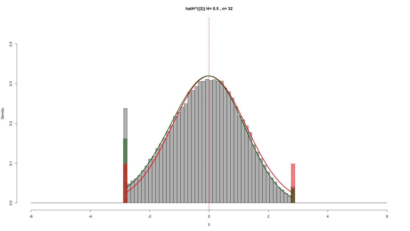
(a) $H=0.5$, $n=32$

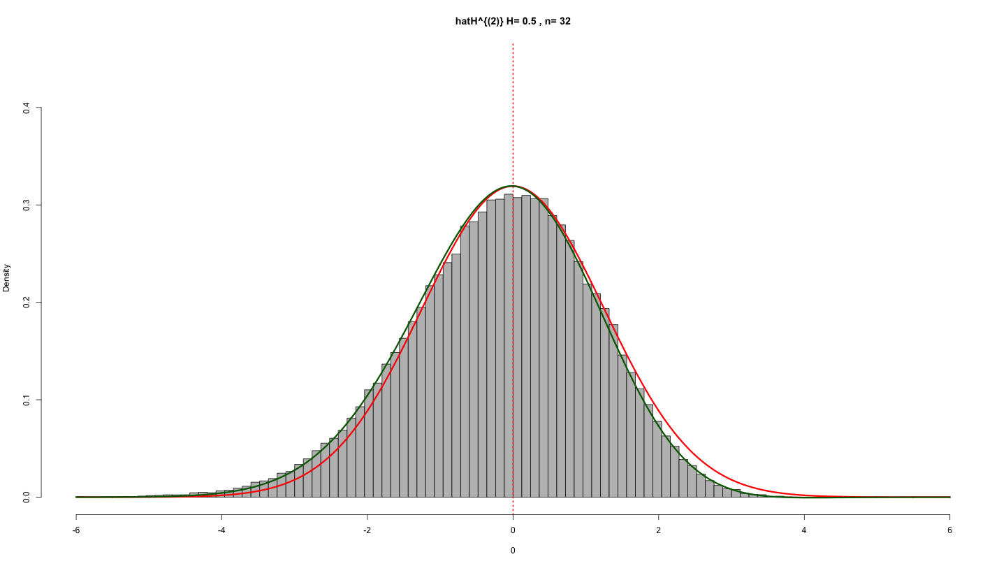
(b) $H=0.5$, $n=32$

When $n$ increases, the atoms become smaller as well as the difference between the asymptotic expansion and the normal approximation decreases.

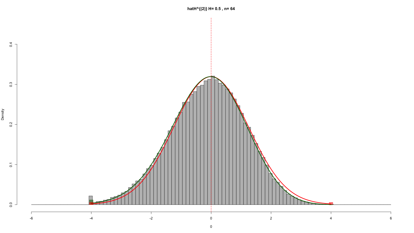
(a) $H=0.5$, $n=64$

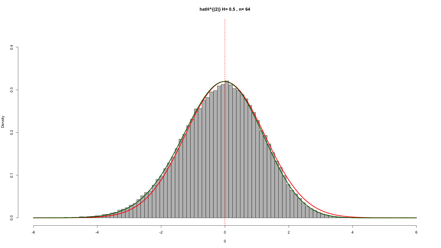
(b) $H=0.5$, $n=64$

Since the precision of approximation of the atoms is determined by that of density, we will leave the curves and omit to draw atoms by the approximations, in the following several plots for different values of $H$. In practical use, the density should be integrated on the tails to approximate the distribution of $\widehat{H}_{n}^{(2)}$ of (1.1), that has atoms on the endpoints $0$ and $1$.

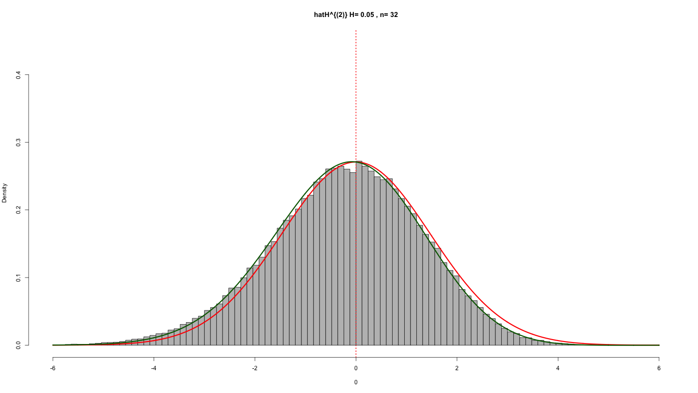
$H=0.05$, $n=32$

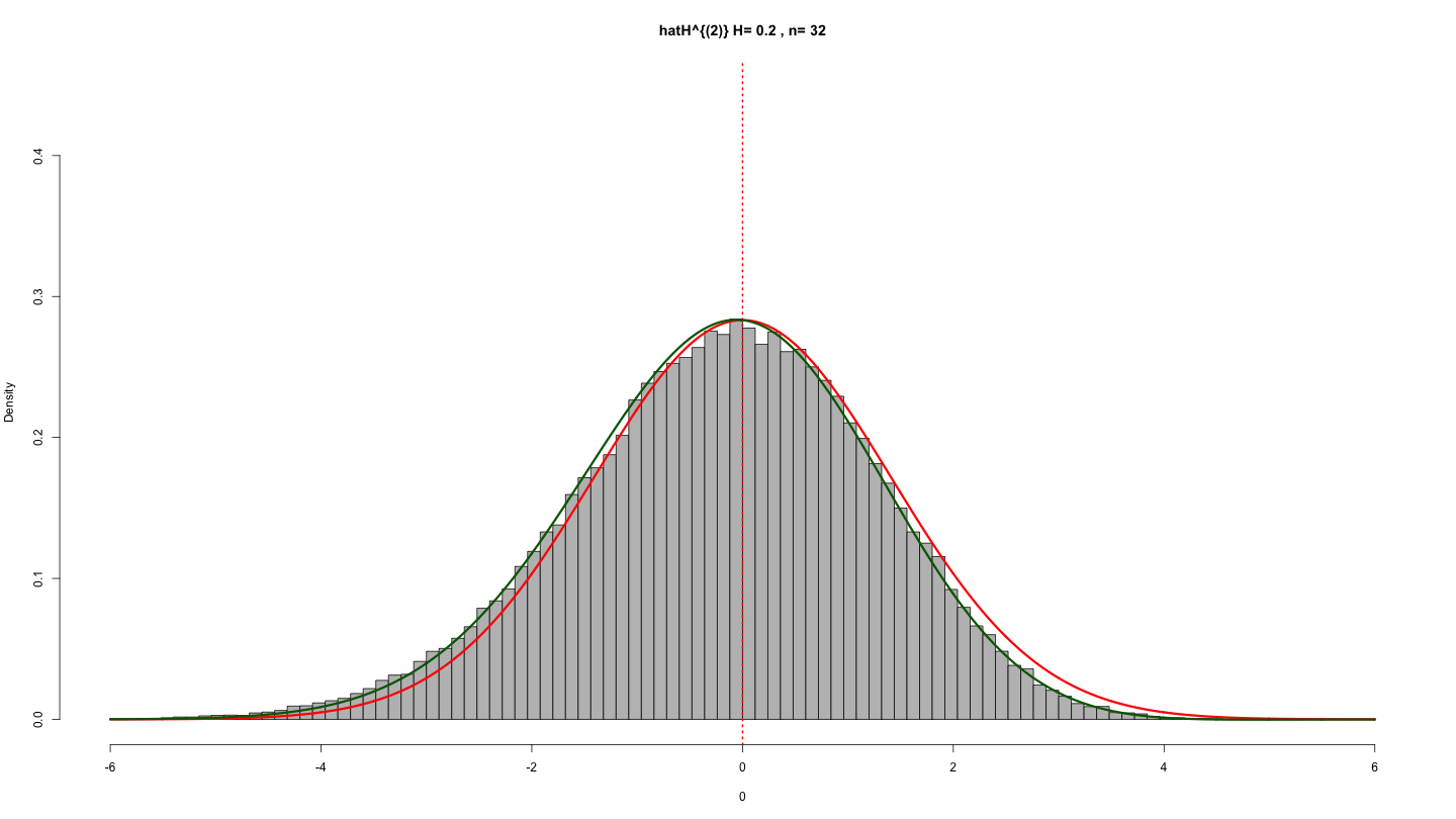
$H=0.20$, $n=32$

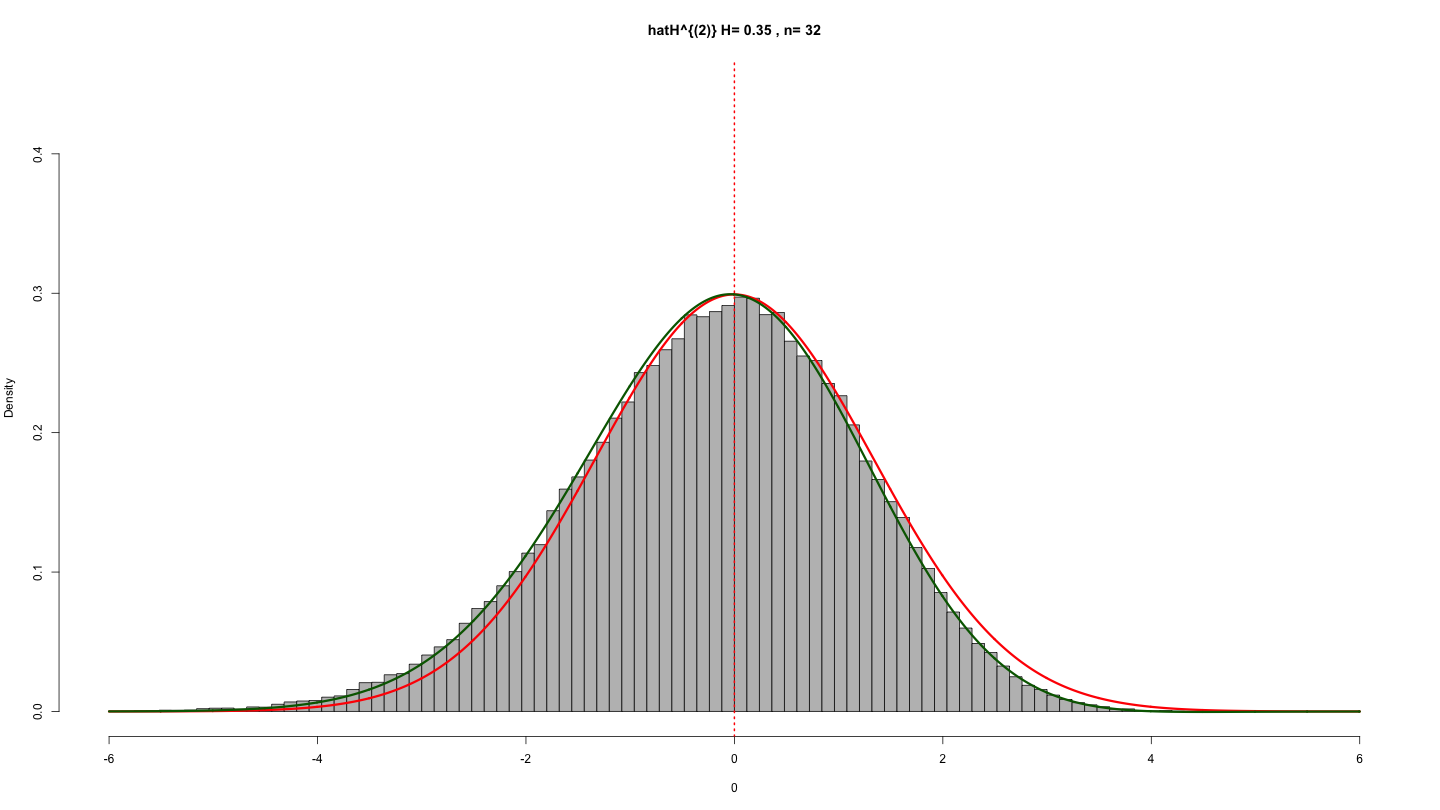
$H=0.35$, $n=32$

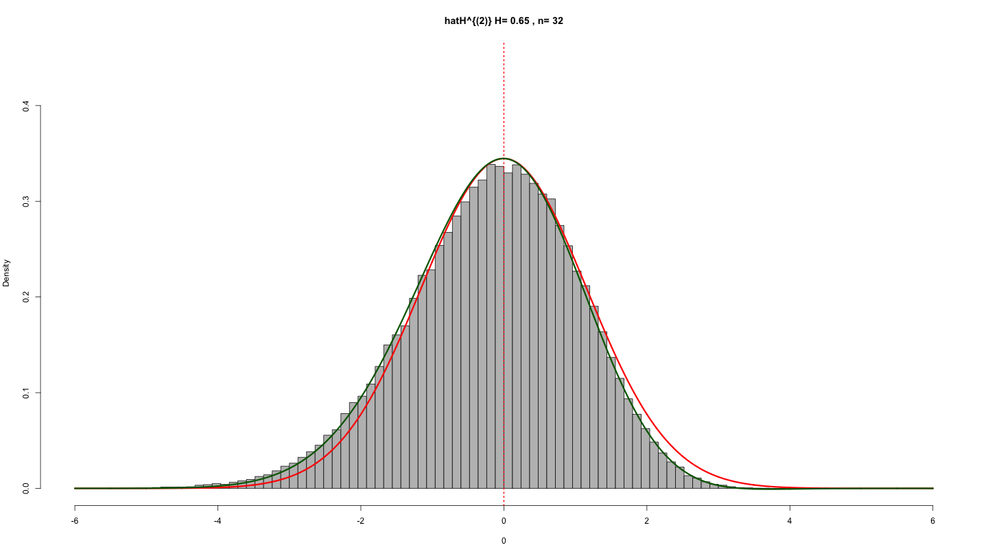
$H=0.65$, $n=32$

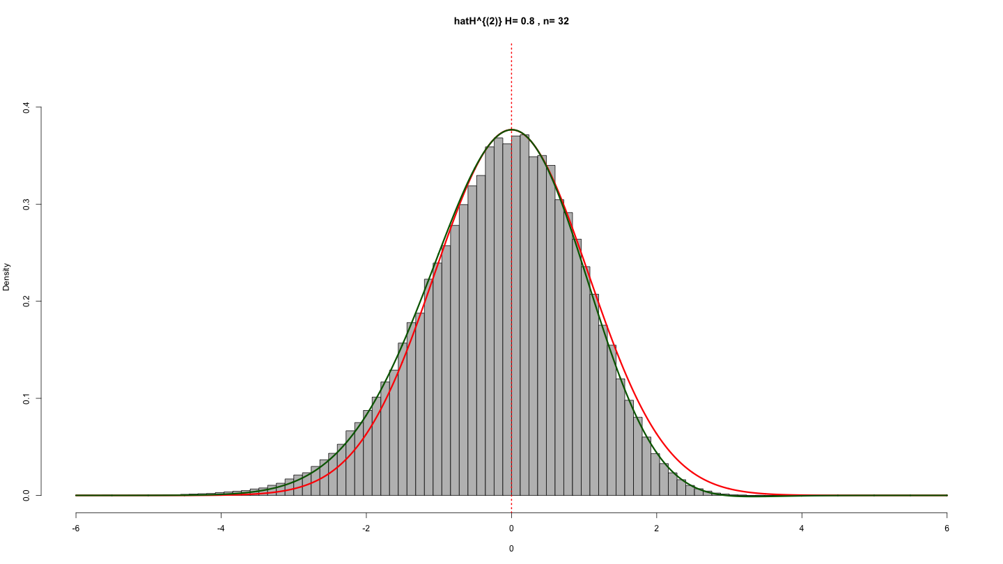
$H=0.80$, $n=32$

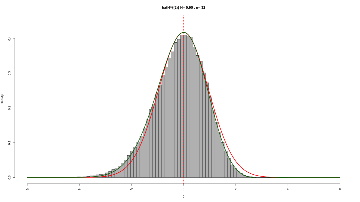
$H=0.95$, $n=32$

References

- [1] Benassi, A., Cohen, S., Istas, J., Jaffard, S.: Identification of filtered white noises. Stochastic Processes and their Applications 75(1), 31–49 (1998)
- [2] Bhattacharya, R., Lin, L., Patrangenaru, V.: A course in mathematical statistics and large sample theory. Springer (2016)
- [3] Bhattacharya, R.N.: Rates of weak convergence and asymptotic expansions for classical central limit theorems. Ann. Math. Statist. 42, 241–259 (1971)
- [4] Bhattacharya, R.N., Ranga Rao, R.: Normal approximation and asymptotic expansions. John Wiley & Sons, New York-London-Sydney (1976). Wiley Series in Probability and Mathematical Statistics
- [5] Cramér, H.: On the composition of elementary errors: First paper: Mathematical deductions. Scandinavian Actuarial Journal 1928(1), 13–74 (1928)
- [6] Cramér, H.: Random variables and probability distributions, vol. 36. Cambridge University Press (2004)
- [7] Gnedenko, B., Kolmogorov, A.: Limit distributions for sums of independent random variables (1954). Cambridge, Mass (1954)
- [8] Ikeda, N., Watanabe, S.: Stochastic differential equations and diffusion processes, North-Holland Mathematical Library, vol. 24, second edn. North-Holland Publishing Co., Amsterdam (1989)
- [9] Istas, J., Lang, G.: Quadratic variations and estimation of the local hölder index of a gaussian process. In: Annales de l’Institut Henri Poincare (B) Probability and Statistics, vol. 33, pp. 407–436. Elsevier (1997)
- [10] Kubilius, K., Mishura, Y., Ralchenko, K.: Parameter estimation in fractional diffusion models, vol. 8. Springer (2018)
- [11] Nourdin, I., Peccati, G.: Normal approximations with Malliavin calculus: from Stein’s method to universality, vol. 192. Cambridge University Press (2012)
- [12] Nualart, D.: The Malliavin calculus and related topics, second edn. Probability and its Applications (New York). Springer-Verlag, Berlin (2006)
- [13] Nualart, D., Peccati, G.: Central limit theorems for sequences of multiple stochastic integrals. The Annals of Probability 33(1), 177–193 (2005)
- [14] Nualart, D., Yoshida, N.: Asymptotic expansion of skorohod integrals. Electronic Journal of Probability 24 (2019)
- [15] Petrov, V.V.: Sums of independent random variables. Springer-Verlag, New York-Heidelberg (1975). Translated from the Russian by A. A. Brown, Ergebnisse der Mathematik und ihrer Grenzgebiete, Band 82
- [16] Sakamoto, Y., Yoshida, N.: Asymptotic expansion under degeneracy. J. Japan Statist. Soc. 33(2), 145–156 (2003)
- [17] Tudor, C.A., Yoshida, N.: Asymptotic expansion for vector-valued sequences of random variables with focus on Wiener chaos. Stochastic Processes and their Applications 129(9), 3499–3526 (2019)
- [18] Tudor, C.A., Yoshida, N.: High order asymptotic expansion for Wiener functionals. arXiv preprint arXiv:1909.09019 (2019)
- [19] Tudor, C.A., Yoshida, N.: Asymptotic expansion of the quadratic variation of a mixed fractional Brownian motion. Statistical Inference for Stochastic Processes 23(2), 435–463 (2020)
- [20] Watanabe, S.: Lectures on stochastic differential equations and Malliavin calculus (Notes by Nair, M Gopalan and Rajeev, B), vol. 73. Springer Berlin et al. (1984)
- [21] Yamagishi, H., Yoshida, N.: Order estimate of functionals related to fractional brownian motion and asymptotic expansion of the quadratic variation of fractional stochastic differential equation. arXiv preprint arXiv:2206.00323 (2022)
- [22] Yoshida, N.: Malliavin calculus and asymptotic expansion for martingales. Probability Theory and Related Fields 109(3), 301–342 (1997)
- [23] Yoshida, N.: Malliavin calculus and martingale expansion. Bulletin des sciences mathematiques 125(6-7), 431–456 (2001)
- [24] Yoshida, N.: Martingale expansion in mixed normal limit. Stochastic Processes and their Applications 123(3), 887–933 (2013)
- [25] Yoshida, N.: Asymptotic expansions for stochastic processes. In: M. Denker, E. Waymire (Eds.) Rabi N. Bhattacharya, pp. 15–32. Springer (2016)
- [26] Yoshida, N.: Asymptotic expansion of a variation with anticipative weights. arXiv:2101.00089 (2020)