How important are activation functions in regression and classification? A survey, performance comparison, and future directions

Abstract

Inspired by biological neurons, the activation functions play an essential part in the learning process of any artificial neural network commonly used in many real-world problems. Various activation functions have been proposed in the literature for classification as well as regression tasks. In this work, we survey the activation functions that have been employed in the past as well as the current state-of-the-art. In particular, we present various developments in activation functions over the years and the advantages as well as disadvantages or limitations of these activation functions. We also discuss classical (fixed) activation functions, including rectifier units, and adaptive activation functions. In addition to discussing the taxonomy of activation functions based on characterization, a taxonomy of activation functions based on applications is presented. To this end, the systematic comparison of various fixed and adaptive activation functions is performed for classification data sets such as the MNIST, CIFAR-10, and CIFAR-100. In recent years, a physics-informed machine learning framework has emerged for solving problems related to scientific computations. For this purpose, we also discuss various requirements for activation functions that have been used in the physics-informed machine learning framework. Furthermore, various comparisons are made among different fixed and adaptive activation functions using various machine learning libraries such as TensorFlow, Pytorch, and JAX. Our findings show that activation functions such as ReLU and its variants, which are currently the state-of-the-art for many classification problems, do not work well in physics-informed machine learning frameworks due to the stringent requirement of the existence of derivatives, whereas other activation functions such as hyperbolic tangent, swish and sine give better performance, with superior results achieved with adaptive activation functions, especially for multiscale problems.

I Introduction

I-A Aim

In recent years, artificial neural networks (ANN) have achieved remarkable success in both academia as well as industry. The ANN has found success in a variety of industries, such as cybersecurity [1, 2], manufacturing technologies [3, 4], healthcare [5], financial services [6], food industry [7], and energy [8], to name a few, where they perform a range of tasks, including logistics, inventory management, etc. With various scientific applications, ANN is now the most sophisticated algorithm for understanding complicated sensory input, such as images [9], video [10], audio [11], etc.  The first computational model for neural networks was created by McCulloch and Pitts [12], whereas the first ANN, also called as Perceptron was invented by Rosenblatt [13]. Ivakhnenko and Lapa [14] released the Group Method of Data Handling, which was the first functional neural network with multiple layers. However, a seminal book written by Minsky and Papert [15] showed that these early neural networks were incapable of processing simple tasks, and computers lacked the capability to process usable neural networks. Early neural networks developed by Rosenblatt only comprised one or two trainable layers. Such simplistic networks cannot mathematically represent complicated real-world phenomena. Deep neural networks (DNN) are ANNs that have a large number of trainable hidden-layers. The DNN was theoretically more versatile. However, without success, researchers spent several years trying to figure out how to train the DNN, as it could not scale with the first neural network’s straightforward hill-climbing algorithm. In a groundbreaking study, Rumelhart et al. [16] created the backpropagation training algorithm to train the DNN. The backpropagation algorithm is used to effectively train any ANN using a gradient descent method that takes advantage of the chain rule. Since then, ANN research has opened up all of the exciting and transformative developments in computer vision [17], speech recognition [18], natural language processing [19], and even in scientific computations called Physics-Informed Machine Learning [20].

Artificial neurons are a set of connected units or nodes in an ANN that loosely replicate the neurons in a biological brain. The Threshold Logic Unit, also known as the Linear Threshold Unit, was the first artificial neuron and was first put forth by McCulloch and Pitts [12] in 1943. The model was intended to serve as a computational representation of the brain’s ’nerve net’. Each artificial neuron receives inputs and generates a single output that can be delivered to a number of other neurons. Artificial neurons do not simply output the raw data they receive. Instead, there is one more step, which is analogous to the rate of action potential firing in the brain and is called an activation function. The introduction of the activation function in ANN was inspired by biological neural networks whose purpose is to decide whether a particular neuron fires or not. The simple addition of such a nonlinear function can tremendously help the network to exploit more, thereby learning faster. There are various activation functions proposed in the literature, and it is difficult to find the optimal activation function that can tackle any problem. In this survey, our aim is to discuss various advantages as well as disadvantages or limitations of classical (fixed) as well as modern (adaptive) activation functions.

I-B Contributions of this work

To the best of our knowledge, this is the first comprehensive survey of activation functions for both classification and regression problems. Apart from that, we also present several original contributions, summarized below.

• First, we have done a comprehensive survey of the classical (fixed) activation functions like the real-valued activation functions, including the rectifier units. This also includes the oscillatory as well as the non-standard activation functions. We further discuss various properties of the classical activation functions that make them best suited for particular tasks.

• We present an applications-based taxonomy of activation functions, which is more suitable from a scientific computation point-of-view. Apart from real-valued activation functions, we also discuss various complex-valued activation functions, which have many applications in remote sensing, acoustics, opto-electronics, image processing, quantum neural devices, robotics, bioinformatics, etc. Furthermore, the quantized activations, which are a special type of activation function, are also discussed in detail. The quantized activations are typically used to improve the efficiency of the network without degrading the performance of the model.

• The state-of-the-art adaptive activation functions, which outperform their classical counterparts, are thoroughly discussed. Such adaptive activation not only accelerates the training of the network but also increases the prediction accuracy. Various adaptive activation functions such as stochastic or probabilistic, ensemble, fractional, etc. are discussed in detail. To this end, we also compare various fixed and adaptive activation functions systematically for classification data sets including MNIST, CIFAR-10, and CIFAR-100.

• Physics-informed machine learning is an intriguing approach that seamlessly incorporates the governing physical laws into the machine learning framework. Such incorporation of physical laws sets additional requirements for the activation function. To this end, we discuss these requirements for specifically solving scientific problems using a physics-informed machine learning framework. We used various fixed and adaptive activation functions to solve different PDEs. Furthermore, we also compare the predictive accuracy of the solution for different activation functions using various machine learning libraries such as TensorFlow, PyTorch, and JAX using clean and noisy data sets. A run-time comparison is made among the TensorFlow, PyTorch, and JAX machine learning libraries.

I-C Organization

This paper is organized as follows: In Section 2, we provide a historical perspective of the activation functions. In section 3, we compare biological and artificial neurons in detail, followed by section 4, where some of the desired features of the neurons are discussed in depth. Section 5 gives a detailed discussion about the taxonomy of the activation functions. Section 6 covers several classical activation functions with their improved versions in detail. Section 7 is devoted to the motivation and historical development of complex-valued activation functions. Similarly, section 8 discusses the efficient quantized activations for quantized neural networks. In Section 9, we discuss various types of adaptive or trainable activation functions, ranging from stochastic or probabilistic to ensemble activations. Various fixed and adaptive activation functions are compared in terms of accuracy for the MNIST, CIFAR-10, and CIFAR-100 data sets in Section 10 using two convolutional neural network-based models, namely, MobileNet and VGG16. Section 11 presents a discussion on the activation function required for solving regression problems using a physics-informed machine learning framework. Finally, we summarize our findings in section 12.

II Activation functions: A historical perspective

The activation function is a function that acts on the output of the hidden layer and the output layer (optional), which helps the neural network to learn complex features of the data. The motivation to employ the activation function came from the biological neural networks where this activation function decides whether the particular neuron activates (fires) or not. The important feature of the activation function is the ability to introduce nonlinearity in the network in order to capture nonlinear features, without which the neural network acts as a linear regression model. Cybenko [21] and Hornik [22] argue for the activation function’s nonlinearity, demonstrating that the activation function must be bounded, non-constant, monotonically rising, and continuous to ensure the neural network’s universal approximation property.

Figure 1 shows some of the notable historical developments related to activation functions that we shall discuss here. In the literature, the term activation function has been referred to with different names, such as squashing function [23], and output function or transfer function [24]. In [25], Dasgupta and Schnitger defined the activation as a real-valued functions defined on subset of $\mathbb{R}^{n}$. In [26], Goodfellow et al. described the activation function as a fixed nonlinear function. The activation function was first used in the work of Fukushima [27] for visual feature extraction in hierarchical neural networks. Later, Fukushima and Miyake [28] proposed it again for visual pattern recognition. Hahnloser et al. [29, 30] argued that the activation function is strongly related to biological neurons. The work of Glorot et al. [31] describes the utility of the ReLU activation function. During the early 1990’s, the Sigmoid activation function [32] was one of the most popular activation functions. Due to its vanishing gradient problem, the notable improvement of Sigmoid such as the improved logistic Sigmoid function [33] has recently been proposed. In the late 1990’s, researchers widely used the hyperbolic tangent function [34] as an activation function. Both Sigmoid and hyperbolic tangent face vanishing gradient problems and have difficulties with large inputs as they saturate for large input values. Later researchers proposed some alternative functions, and one of the most popular gradient vanishing-proof activation functions was the rectified linear unit (ReLU). As of 2017, the ReLU was the most popular activation function [35] compared to widely used activation functions such as sigmoid and hyperbolic tangent functions. Although the ReLU was very successful in many applications such as speech recognition [36] and computer vision [31], it suffered from issues such as non-differentiability at zero, unboundedness, and the most famous, the dying ReLU problem [36]. Several other linear as well as non-linear variants of the rectifier unit were proposed. The notable ones are leaky ReLU [36] and parametric ReLU [37], which are linear variants. Some of the non-linear variants are softplus [38], Exponential linear units (ELU) [39], Gaussian Error Linear Units (GELU) [40], Swish [35] and Mish [41].

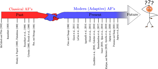
Figure 1: Notable historical developments over the years related to the activation function.

Recent years have seen an increase in studies on adaptive activation functions. In the early studies, the generalized hyperbolic tangent function was suggested by Chen and Chang [42]. It is parameterized by two additional positive scalar values. Vecci et al. [43] proposed an adaptive spline activation function. Trentin [44] gives empirical evidence that learning the amplitude for each neuron is superior to having a unit amplitude for all activation functions  (either in terms of generalization error or speed of convergence). Goh et al. [45]  proposed a trainable amplitude activation function. The activation function adaptation algorithm is suggested for sigmoidal feed-forward neural network training by Chandra and Singh [46]. Recently,  Agostinelli et al.  [47] proposed learning activation functions. Eisenach et al. [48]  proposed a nonparametric method for learning activation functions. The algebraic activation functions were proposed by Babu and Edla [49]. Urban et al. proposed stochastic activation functions based on Gaussian processes in [50]. Alcaide et al. [51] proposed the E-swish activation function. The trained activation function was proposed by Ertuğrul [52]. Convolutional neural networks with adaptive activations were proposed by Qian et al. [53]. In order to discover the ideal quantization scale, Choi et al. [54] introduced PArameterized Clipping acTivation (PACT), which makes use of an activation clipping parameter that is tuned during training. Apicella et al. [55] proposed an effective design for trainable activation functions. Several variants of adaptive ReLU activation function have been proposed recently, such as Parametric ReLU [37], S-shaped ReLU [56], Flexible ReLU [57], Paired ReLU [58], etc. Similarly, adaptive ELUs like Parametric ELU [59], Continuously Differentiable ELU [60], Shifted ELU [61], Fast ELU [62], Elastic ELU [63], etc. are also proposed in the literature. Recently, Jagtap et al. proposed a series of papers on global [64] and local [65] adaptive activation functions. The other way to introduce adaptivity is through the use of stochastic activation functions. Gulcehre et al. [66] proposed a noisy activation function where a structured bounded noise-like effect is added to allow the optimizer to exploit more and learn faster. On a similar idea, Shridhar [67] proposed the probabilistic activation functions, which are not only trainable but also stochastic in nature. In this work, the authors replicated uncertain behavior in the information flow to the neurons by injecting stochastic sampling from a normal distribution into the activations. The fractional activation functions with trainable fractional parameters are proposed by Ivanov [68]. Later, Esquivel et al. [69] provided adaptable activation functions based on fractional calculus. The ensemble technique is another way to adapt activation functions. The earlier work of Xu and Zhang [70] proposes an adaptive ensemble activation function consisting of sigmoid, radial basis, and sinusoid functions. In [71], Ismail et al. select the most suitable activation function as a discrete optimization problem that involves generating various combinations of functions. Chen [72] used multiple activation functions for each neuron for the problems related to stochastic control. Agostinelli et al. [47] constructed the activation functions during the network training. Jin et al. [56] proposed the combination of a set of linear functions with open parameters. In recent years, a generalized framework, namely Kronecker Neural Networks for any adaptive activation functions, has been proposed by Jagtap et al. [73]. Good reviews of classical activation functions [74, 75] and the modern trainable activation [76] are available for various classification problems.

III Biological vs artificial neurons

A neuron in the human brain is a biological cell that processes information. The biological neuron is depicted in the top figure 2. There are three basic elements of a biological neuron. The dendrites receive singles $x_{i},i=1,2,\cdots,n$ as an input from other neurons. A cell body (nucleus) that controls the activity of neurons and an axon that transmits signals to the neighboring neurons. The axon’s length may be several times or even tens of thousands of times longer than the cell body. The axon is divided into various branches near its extremity, which are connected to the dendrites of other neurons. There are millions of massively connected neurons (around $10^{11}$), which is approximately equal to the number of stars in the Milky way [77]. Every neuron is connected to thousands of neighboring neurons, and these neurons are organized into successive layers in the cerebral cortex.

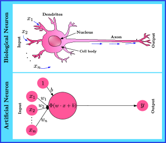
Figure 2: Biological (top) vs artificial (bottom) neurons.

Such a massively parallel neural network communicates through a very short train of pulses, in milliseconds, and has an ability that includes parallel processing, fast learning ability, adaptivity, generalization ability, very low energy consumption, and fault tolerance.  The artificial neuron in the bottom figure 2 attempts to resemble the biological neuron. The artificial neuron, like a biological neuron, takes input $x_{i},i=1,2,\cdots,n$, and is made up of three basic parts: weights $w$ and bias $b$, which act as a dendrites, the activation function (denoted by $\Phi(\cdot)$) that act as a cell body and nucleus, and the output $y$. The artificial neuron has been generalized in many ways. Among all the components, the most obvious is the activation function. The activation function plays an important role in replicating the biological neuron firing behaviour above some threshold value. Unlike biological neurons, which send binary values, artificial neurons send continuous values, and depending on the activation function, the firing behavior of artificial neurons changes significantly.

IV Desired characteristics of the activation functions

There is no universal rule for determining the best activation function; it varies depending on the problem under consideration. Nonetheless, some of the desirable qualities of activation functions are well known in the literature. The following are the essential characteristics of any activation function.

1. Nonlinerity: One of the most essential characteristics of an activation function is nonlinearity. In comparison to linear activation functions, the non-linearity of the activation function significantly improves the learning capability of neural networks. In [21] Cybenko and [22] Hornik advocates for the nonlinear property of the activation function, demonstrating that the activation function must be bounded, non-constant, monotonically growing, and continuous in order to ensure the neural network’s universal approximation property. In [78, 79] Morita later discovered that neural networks with non-monotonic activation functions perform better in terms of memory capacity and retrieval ability. Recently, Sonoda and Murata [80] showed that neural networks equipped with unbounded but non-polynomial activation functions (e.g., ReLU) are universal approximators.

2. Computationally cheap: The activation function must be easy to evaluate in terms of computation. This has the potential to greatly improve network efficiency.

3. The vanishing and exploding gradient problems: The vanishing and exploding gradient problems are the important problems of activation functions. The variation of the inputs and outputs of some activation functions, such as the logistic function (Sigmoid), is extremely large. To put it another way, they reduce and transform a bigger input space into a smaller output space that falls between [0,1]. As a result, the back-propagation algorithm has almost no gradients to propagate backward in the network, and any residual gradients that do exist continue to dilute as the program goes down through the top layers. Due to this, the initial hidden-layers are left with no information about the gradients. For hyperbolic tangent and sigmoid activation functions, it has been observed that the saturation region for large input (both positive and negative) is a major reason behind the vanishing of gradient. One of the important remedies to this problem is the use of non-saturating activation functions. Other non-saturating functions, such as ReLU, leaky ReLU, and other variants of ReLU, have been proposed to solve this problem.

4. Finite range/boundedness: Gradient-based training approaches are more stable when the range of the activation function is finite, because pattern presentations significantly affect only limited weights.

5. Differentiability: The most desirable quality for using gradient-based optimization approaches is continuously differentiable activation functions. This ensures that the back-propagation algorithm works properly.

V Taxonomy of activation functions

V-A Characterization based taxonomy

A taxomomy of activation functions was proposed in [76], which we also follow in the current work. Specifically, the activation functions can be broadly divided into linear and nonlinear functions. For all realistic problems, nonlinear activation functions are often employed.

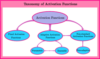
Figure 3: Taxonomy based on characterization of activation functions: The activation functions are broadly divided into three categories, namely, fixed, adaptive, and non-standard activation functions. There are various ways to inject the adaptive nature of the activation function, like ensemble or parametric approaches. The non-standard activation functions can be fixed or adaptive.

Figure 3 shows the taxonomy based on characterization of activation functions, which divides the activation function into three major categories, first is the fixed activation function (see Section VI) that contains all the fixed (classical) activations, including the rectifier units. The second category is the adaptive or modern activation functions that can adapt itself, which is further divided into parametric as well as ensemble activations. The third category is non-standard activation, such as multi-fold activation from previous layers, which may be fixed or adaptive.

V-B Application based taxonomy

Although the taxonomy of activation functions based on their characterization encompasses all the activation functions, it is possible to define the taxonomy based on their applications to real-world problems; this can help us to further broaden our understanding of activation functions from a physical point-of-view. In particular, we are proposing an application-based taxonomy for scientific applications, where the output field states are real or complex-valued; for example, applications in acoustics, robotics, and bioinformatics may include complex arithmetic representation. A schematic representation of this is shown in Fig. 4. The real-valued activations are well-known in the literature, and we shall discuss them in detail later. The complex-valued activation functions are another set of activation functions whose output is a complex number. These activation functions are often required due to the complex-valued output, which has many applications in science and engineering, such as bioinformatics, acoustics, robotics, opto-electronics, quantum neural devices, image processing, etc.

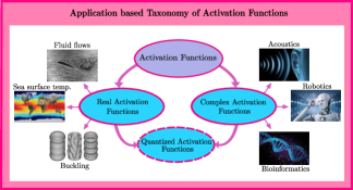
Figure 4: Taxonomy based on the application of activation functions: The activation function can also be divided based on the application at hand and the nature of its output. In particular, we propose real and complex-valued activation functions. Few scientific applications of such activation functions are also shown in the taxonomy. For efficient computation, both real and complex-valued activation functions can be quantized.

The process of mapping continuous values from an infinite set to discrete finite values is known as Quantization. Both real and complex-valued activation functions can be quantized in order to reduce memory requirements. Quantized activations are the class of activation functions that is efficient in terms of memory requirements as well as increased compute efficiency. The output of the quantized activation is integers rather than floating point values. Note that, just like real-valued activation functions, both complex-valued as well as quantized activations can be made adaptive by introducing the tunable variables. The upcoming sections provide a clear discussion of the various complex-valued and quantized activation functions.

VI Classical activation functions in artificial neural networks

This section gives details about the various fixed activation functions that have been proposed in the literature. These activation functions do not contain any tunable parameters. The following are the most common fixed activation functions used.

VI-A Linear and piece-wise linear functions

Linear function $\Phi(x)=x$ is the simplest form of activation function. It has a constant gradient, and the descent is based on this constant value of gradient. The range of linear function is $(-\infty,\infty)$, and has a $C^{1}$ order of continuity.

The piece-wise linear activation can be defined as

$$\Phi(x)=\begin{cases}0&x<-b,\\ x+b&-b<x<b,\\ 1&x>b,\end{cases}$$

where $b$ is a constant. The derivative of piece-wise linear activation is not defined at $x=\pm b$, and it is zero for $x<-b$ and $x>b$. The linear function has a $C^{0}$ order of continuity and a range of $[0,1]$.

VI-B Step function

It is also known as Heaviside or the unit step function, and is defined as

$$\Phi(x)=\begin{cases}0&\text{for}~{}x<0\\ 1&\text{for}~{}x\geq 0.\end{cases}$$

Step function is one of the most basic forms of activation function. The derivative of a step function is zero when $x\neq 0$, and it is not defined when $x=0$. The step function has a $C^{-1}$ order of continuity and a $\{0,~{}1\}$ range.

VI-C Sigmoid function

The sigmoid function [32], also called the logistic function, was a very popular choice of activation function till the early 1990’s. It is defined as

$$\Phi(x)=\frac{1}{1+e^{-x}}.$$

In [81], Hinton et al. used a sigmoid activation function for automatic speech recognition. The major advantage of sigmoid activation is its boundedness. The disadvantages are: the vanishing gradient problem, the output not being zero-centered, and the saturation for large input values. In [82], Nair and Hinton showed that as networks became deeper, training with sigmoid activations proved less effective. The range of the sigmoid function is [0,1] and has a $C^{\infty}$ order of continuity.

Some improvements to Sigmoid functions were proposed in the literature as follows.

• The Bipolar-Sigmoid activation function [83] is defined as

  $$\Phi(x)=\frac{1-e^{-x}}{1+e^{-x}},$$

  which has a range of [-1,1]. Bipolar sigmoid activation function is widely used in Hopfield neural network, see for more details in [84].

• The Elliott function defined in [85] has a similar structure as the Sigmoid function and it is given by

  $$\Phi(x)=\frac{0.5x}{1+|x|}+0.5,$$

  with range [0,1]. See [86] for more details.

• The parametric sigmoid function [46] is given by

  $$\Phi(x)=\left(\frac{1}{(1+\text{exp}(-x))}\right)^{m},~{}~{}m\in(0,\infty).$$

  The derivatives for $m\neq 1$ are skewed and their maxima shift from the point corresponding to the input value equal to zero.

• An improved logistic Sigmoid function is proposed by [33] to overcome the vanishing gradient problem as

  $$\Phi(x)=\begin{cases}\alpha(x-a)+\text{Sigmoid}(a),&x\geq a,\\ \text{Sigmoid}(x),&-a<x<a,\\ \alpha(x+a)+\text{Sigmoid}(a),&x\leq a,\end{cases}$$

  which has a [$-\infty,\infty$] range.

• The scaled sigmoid function [87] is defined as

  $$\Phi(x)=\frac{4}{1+\text{exp}(-x)}-2,$$

  which has a range from [-2,2].

VI-D Hyperbolic tangent (tanh) function

The tanh activation function is defined as

$$\Phi(x)=\frac{e^{x}-e^{-x}}{e^{x}+e^{-x}}.$$

From the late 1990’s till early 2000s, tanh was extensively used to train neural networks, and was a preferred choice over the classical sigmoid activation function. The tanh activation has a range of $[-1,~{}1]$, and in general, is mostly used for regression problems. It has an advantage due to the zero-centered structure. The main problem with the tanh activations is the saturation region. Once saturated, it is really challenging for the learning algorithm to adapt the parameters and learn faster. This problem is the vanishing gradient problem.

Some improved tanh activation functions have been proposed to eliminate the problems related to the original tanh activation function.

• A scaled hyperbolic tangent function is defined by [88] as

  $$\Phi(x)=A~{}\tanh(S~{}x).$$

  Here $A$ is the amplitude of the function, and $S$ determines its slope at the origin. The output of the activation function is the range $[-A,A]$.

• A rectified hyperbolic secant activation function [89] is proposed as $\Phi(x)=x~{}\text{sech}(x)$.

• The Hexpo function [90] has a similar structure to the hyperbolic tangent function, which is defined as

  $$\Phi(x)=\begin{cases}-a~{}(\text{exp}(-x/b)-1),&x\geq 0,\\ c~{}(\text{exp}(-x/d)-1),&x<0,\end{cases}$$

  and has range from [$-c,a$].

• The penalized hyperbolic tangent function [87] is defined as

  $$\Phi(x)=\begin{cases}\tanh(x),&x\geq 0,\\ a~{}\tanh(x)&x<0,\end{cases}$$

  which gives output in the range [$-a,1$].

• The linearly scaled tanh (LiSHT) activation function [91] is defined as $\Phi(x)=x~{}\tanh(x)$. The LiSHT scales the hyperbolic tangent function linearly to tackle its gradient diminishing problem.

VI-E Rectified Linear Unit (ReLU)

ReLU was primarily used to overcome the vanishing gradient problem. ReLU is the most common activation function used for classification problems. It is defined as

$$\Phi(x)=\begin{cases}0&\text{for}~{}x\leq 0\\ x&\text{for}~{}x>0.\end{cases}$$

The derivative of ReLU is zero when $x<0$, unity when $x>0$, and at $x=0$, the derivative is not defined. The ReLU function has a range from $[0,~{}\infty)$ and has a $C^{0}$ order of continuity. Apart from overcoming the vanishing gradient problem, the implementation of ReLU is very easy and thus cheaper, unlike tanh and sigmoid, where an exponential function is needed. Despite having some advantages over classical activations, ReLU still has a saturation region, which can prevent the learning of the networks. In particular, ReLU always discards the negative values. This makes the neurons stop responding to the gradient-based optimizer. This problem is known as dead or dying ReLU problem [36, 92], meaning the neurons stop outputting other than zero. This is one of the serious problems for ReLU, where most of the neurons become dead, especially when using a high learning rate. To overcome these problems, various variants of ReLU have been proposed.

• Leaky ReLU [36]: The leaky ReLU is defined as

  $$\Phi(x)=\begin{cases}\alpha x&\text{for}~{}x\leq 0\\ x&\text{for}~{}x>0.\end{cases}$$

  The hyperparameter $\alpha$ defines the leakage in the function (slope of the function). By adding the small slope in the region $x<0$, the leaky ReLU overcomes the dying ReLU problem. Moreover, it has all the advantages of ReLU activation. One of the disadvantage of leaky ReLU is the hyperparameter $\alpha$, which needs to be defined appropriately. In most of the cases $\alpha=0.01$ is used. In [93], Xu et al. compared the ReLU and leaky ReLU activation with the conclusion that the latter outperforms the former always.

• Randomized leaky ReLU [93]: In this case, the $\alpha$ is picked randomly in a given range during training and is fixed to its average value during testing.

• Mirror ReLU [94]: It is defined as

  $$\Phi(x)=\begin{cases}1+x,&-1\leq x\leq 0\\ 1+x,&0<x\leq 1\\ 0,&\text{Otherwise},\end{cases}$$

  which can also be defind as $\Phi(x)=\text{min}(\text{ReLU}(1-x),\text{ReLU}(1+x))$.

• Concatenated ReLU [95]: The concatenated ReLU (CReLU) is given as

  $$\Phi(x)=[\text{ReLU}(x),\text{ReLU}(-x)],$$

  which has range of [$0,\infty$). The disadvantage of CReLU over ReLU is increased model complexity.

• Elastic ReLU [96]: The Elastic ReLU is defined as

  $$\Phi(x)=\text{max}(Rx,0),$$

  where $R$ is the random number.

• Bounded ReLU [97]: The ReLU function has unbounded outputs for non-negative inputs. The bounded version of the ReLU function is defined as

  $$\Phi(x)=\text{min}(\text{max}(0,x),A),$$

  where $A$ is the maximum output value the function can produce.

• V-shaped ReLU [98]: It is defined as

  $$\Phi(x)=\begin{cases}x,&x\geq 0\\ -x,&x<0,\end{cases}$$

• Dual ReLU [99]: The Dual ReLU has two dimensions, and it is defined as

  $$\Phi(x)=\text{max}(0,a)-\text{max}(0,b),$$

  where $a,b$ are the inputs in two different dimensions. The range of Dual ReLU is $(-\infty,\infty)$.

• Randomly translated ReLU [100]: It is given by

  $$\Phi(x)=\begin{cases}x+\alpha,&x+\alpha>0\\ 0,&x+\alpha\leq 0,\end{cases}$$

  which has range of [$0,\infty$), where $\alpha$ is randomly sampled from Gaussian distribution.

• Displaced ReLU (DReLU) [101]: DReLU is a diagonally displaced ReLU function that generalizes both ReLU and SReLU [39] by allowing its inflection to move diagonally from the origin to any point of the form. It is defined as

  $$\Phi(x)=\begin{cases}x,&x\geq-\delta\\ -\delta,&x<-\delta,\end{cases}$$

  with range [$-\delta,\infty$). If $\delta=0$ DReLU becomes ReLU, and if $\delta=1$ DReLU becomes SReLU.

• Natural-Logarithm ReLU [102]: The Natural-Logarithm ReLU uses a logarithmic function to modify ReLU output for positive input values that increase the degree of nonlinearity. It is defined as

  $$\Phi(x)=\text{ln}(\beta~{}\text{max}(0,x)+1).$$

  This activation has output range from 0 to $\infty$, and the $\beta$ is constant.

• Average Biased ReLU [103]: The Average-Biased ReLU is given by

  $$\Phi(x)=\begin{cases}x-\beta,&x-\beta\geq 0\\ 0,&\text{Otherwise},\end{cases}$$

  which has range of [$0,\infty$), and the variable $\beta$ is the average of input activation map to activation function.

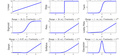
Figure 5: Classical (fixed) activation functions with their range and continuity.

Figure 6: Derivatives of classical activation functions.

VI-F Gaussian Error Linear Units (GELUs)

In GELU activation [40] the neuron input $x$ is multiplied by $m\sim\text{Bernoulli}(P(X\leq x))$ where $X\sim\mathcal{N}(0,1)$. The reason for choosing the Bernoulli distribution is that the neuron’s input follows a normal distribution, especially after batch normalization. The output of any activation function should be deterministic and not stochastic. So, the expected value of the transformation can be found as

$$\mathbb{E}(xm)=x\mathbb{E}=xP(X\leq x).$$

Since $P(X\leq x)$ is a cumulative distribution of Gaussian distribution, it is frequently computed with the error function. Thus, GELU activation is defined as

$$\Phi(x)=x~{}[1+\text{erf}(x/2)],$$

which can be approximated as $0.5x(1+tanh[\sqrt{2/\pi}(x+0.044715~{}x^{3})])$.

To improve its capacity for bidirectional convergence, the GELU was upgraded to the symmetrical GELU (SGELU) by Yu and Su [104].

VI-G Softplus function

The softplus function [38] approximates the ReLU activation function in a smooth way, and it is defined as

$$\Phi(x)=\text{ln}(1+\text{exp}(x)),$$

Softplus function is infinitely differentiable, and it has a range from $(0,\infty$). In [105], Liu and Fuber proposed the noisy softplus activation. With Noisy Softplus, which is well-matched to the response function of LIF (Leaky Integrate-and-Fire) neurons, the performance of spiking neural networks can be improved, see [106]. The authors of [105] proposed the following formula:

$$\Phi(x)=k\sigma~{}\text{ln}\left(1+\text{exp}\left(\frac{x}{k\sigma}\right)\right),$$

where $x$ is the mean input, $\sigma$ defines the noise level, and $k$ controls the curve scaling that can be determined by the neuron parameters.

VI-H Exponential linear unit

The Exponential linear unit (ELU) was first proposed in [39] by Clevert et al., where they show that ELU outperforms all variants of ReLU with reduced training time as well as better accuracy in testing. The ELU is defined as

$$\Phi(x)=\begin{cases}\alpha(\text{exp}(x)-1)&\text{for}~{}x\leq 0\\ x&\text{for}~{}x>0.\end{cases}$$

When $x<0$, it takes on negative values, allowing the unit’s average output to be closer to zero and alleviating the vanishing gradient problem. Also, due to the non-zero gradient for $x<0$, ELU does not suffer from the problem of dead neurons. Unlike ReLU, ELU bends smoothly at origin, which can be beneficial in the optimization process. Similar to leaky ReLU and parametric ReLU, ELU gives a negative output, which pushes the mean value towards zero. Again, $\alpha$ is a parameter which needs to be specified. For $\alpha=1$, the function is smooth everywhere, which in turn helps the gradient descent algorithm to speed up.

In [107], Klambauer et al. proposed the Scaled ELU (SELU) activation function, where the authors show that for the neural network consisting of a stack of dense layers, the network will self-normalize if all the hidden-layers use the SELU activation function. However, there are some conditions for self-normalization; see [107] for more details.

Activation Function ($\mathbf{\Phi(x)}$)	Derivatives ($\mathbf{\Phi^{\prime}(x)}$)	Range	Continutity
Linear : $\Phi(x)=x$	$\Phi^{\prime}(x)=1$	($-\infty,\infty$)	$C^{\infty}$
Step : $\Phi(x)=\begin{cases}0&x\leq 0,\\ 1&x>0\end{cases}$	$\Phi^{\prime}(x)=\begin{cases}0&x\neq 0,\\ \text{Not defined}&x=0\end{cases}$	($0,1$)	$C^{-1}$
Sigmoid or Logistic : $\Phi(x)=\frac{1}{1+e^{-x}}$	$\Phi^{\prime}(x)=\Phi(x)(1-\Phi(x))$	($0,1$)	$C^{\infty}$
Rectifier Unit (ReLU) : $\Phi(x)=\begin{cases}0&x\leq 0,\\ x&x>0\end{cases}$	$\Phi^{\prime}(x)=\begin{cases}0&x<0,\\ 1&x>0,\\ \text{Not defined}&x=0\end{cases}$	[$0,\infty$)	$C^{0}$
Hyperbolic Tangent : $\Phi(x)=\frac{e^{x}-e^{-x}}{e^{x}+e^{-x}}$	$\Phi^{\prime}(x)=1-\Phi(x)^{2}$	($-1,1$)	$C^{\infty}$
Softplus : $\Phi(x)=\text{ln}(1+e^{x})$	$\Phi^{\prime}(x)=~{}\text{Sigmoid}$	($0,\infty$)	$C^{\infty}$
Leaky Rectifier Unit (Leaky ReLU) : $\Phi(x)=\begin{cases}0.01x&x<0,\\ x&x\geq 0\end{cases}$	$\Phi^{\prime}(x)=\begin{cases}0.01&x<0,\\ 1&x>0,\\ \text{Not defined}&x=0\end{cases}$	($-\infty,\infty$)	$C^{0}$
Exponential Linear Unit (ELU) : $\Phi(x)=\begin{cases}\alpha(e^{x}-1)&x\leq 0,\\ x&x>0\end{cases}$	$\Phi^{\prime}(x)=\begin{cases}\alpha e^{x}&x<0,\\ 1&x>0,\\ \alpha&x=0\end{cases}$	($-\alpha,\infty$)	$\begin{cases}C^{1}&\text{If}\alpha=1\\ C^{0}&\text{Otherwise}\end{cases}$
Gaussian : $\Phi(x)=e^{-x^{2}}$	$\Phi^{\prime}(x)=-2x\Phi(x)$	($0,1$]	$C^{\infty}$
Swish ($\beta=1$) : $\Phi(x)=x\cdot\text{Sigmoid}$	$\Phi^{\prime}(x)=x\cdot\Phi(x)(1-\Phi(x))+\text{Sigmoid}$	[$0,.\infty$)	$C^{\infty}$
Oscillatory : $\Phi(x)=\sin(x)$	$\Phi^{\prime}(x)=-\cos(x)$	[$-1,1$]	$C^{\infty}$

TABLE I: Various classical activation functions, their derivatives, range, and order of continuity.

VI-I Mish function

The Mish [41] is a self-regularized, non-monotonic activation function defined as

$$\Phi(x)=x\cdot\tanh(\text{softplus}(x)).$$

While not evident at first sight, Mish is closely related to Swish [35], as its first derivative can be written in terms of the Swish function. Similar to Swish, Mish is unbounded above and bounded below. It is non-monotonic, has $C^{\infty}$ continuity, and is also self-gated.

VI-J Radial activation functions

The traditional radial basis function (RBF) neural networks uses the Gaussian function, which is given as

$$\Phi(x)=e^{-x^{2}}.$$

The RBF neural networks with Gaussian activation functions have previously been successfully applied to a variety of difficult problems such as function approximation [108, 109], classification [110, 111] , etc. In [112], Zhang and Suganthan found that radial basis function always leads to a better performance compared to hardlim and sign activation functions for UCI datasets using Random Vector Functional Link Networks (RVFL) [113]. Other radial activation functions include Multiquadratics [114], and Polyharmonic splines. The polyharmonic spline is a linear combination of polyharmonic radial basis functions and can be used as an activation function [115].

Table I summarises the comparison of different activation functions, their derivatives, range, and order of continuity. The existence of the derivatives is an important feature for the backpropagation algorithm. Figures 5 and 6 show some of the classical activation functions and their derivatives, respectively.

VI-K Wavelet activation functions

Wavelet neural networks [116] use wavelets as the activation function. Such networks have been utilized with some success in classification and identification problems. Moreover, these networks are effective because they can identify important features in high-frequency signals. A good review of wavelet networks and wavelets as activation functions can be found in [117]. The Gaussian-wavelet type activation function is a class of piecewise linear, non-monotone activation functions [37], that have been employed in [118, 119].

VI-L Oscillatory activation functions

In [120], Gidon et al. found a new form of neuron in the human cortex that can learn the XOR function individually (a task that is difficult with single neurons employing other standard activation functions such as sigmoidal, ReLU, leaky ReLU, Softplus, ELU, Swish, Mish activations, etc). This is due to the fact that the zeros of the activation function for which $\Phi(x)=0$ is the decision boundary for a neuron that emits an activation $\Phi(x)=\Phi(w\cdot x+b)$. If the activation function $\Phi(x)$ has only one zero, then the decision boundary is a single hyperplane $x=w\cdot x+b=0$. Two hyperplanes are required to distinguish the classes in the XOR data set [15], hence activation functions with multiple zeros, as described in [121], must be considered. The oscillatory activation functions fits this criterion perfectly. It is interesting to note that oscillatory activation functions were already present in the literature before the paper by Gidon et al. [120]. In [122], Nakagawa proposed the chaos neural network model applied to the chaotic autoassociation memory using sinusoidal activation function. Mingo et al. [123] proposed the Fourier neural network with sinusoidal activation function, see also Gashler and Ashmore [124]. In [125], Parascandolo et al. used sine activation for deep neural networks. For learning the XOR function with a single neuron, Noel et al. [126] proposed the Growing Cosine Unit (GCU) $\Phi(x)=x\cdot\cos(x)$.

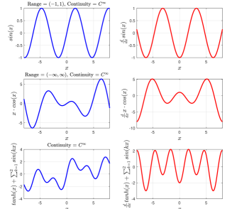
Figure 7: The oscillatory activation functions (first column), and their derivatives (second column).

Figure 7 shows various oscillatory activation functions along with their derivatives. Recently, Jagtap et al. [73] proposed the Rowdy activation function, where the oscillatory noise is injected over the monotonic base activation function with adaptable parameters, thereby making them oscillatory as the optimization process starts. This adaptively creates multiple hypersurfaces to better learn the data set.

VI-M Non-standard activation functions

This section will cover the Maxout unit and the Softmax functions, which are two non-standard activation functions.

• Maxout [127] : The Maxout Unit is a piece-wise linear function that gives the maximum of the inputs, and it is designed to be used in conjunction with dropout [128]. It generalizes the ReLU and leaky ReLU activation functions. Given the units input $x\in\mathbb{R}^{d}$ the activation of a maxout unit is computed by first computing $k$ linear feature mappings $z\in\mathbb{R}^{k}$ where

  $$z_{i}=w_{i}x+b_{i},$$

  and $w_{i},b_{i}$ are weights and biases, whereas $k$ is the number of linear sub-units combined by one maxout unit. Later, the output $h_{\text{maxout}}$ of the maxout hidden unit is given as the maximum over the $k$ feature mappings:

  $$h_{\text{maxout}}(x)=\text{max}[z_{1},...,z_{k}].$$

  Maxout’s success can be partly attributed to the fact that it supports the optimization process by preventing units from remaining idle; a result of the rectified linear unit’s thresholding. The activation function of the maxout unit, on the other hand, can be viewed as executing a pooling operation across a subspace of k linear feature mappings (referred to as subspace pooling in the following). Each maxout unit is somewhat invariant to changes in its input as a result of this subspace pooling procedure. In [129], Springenberg and Riedmiller proposed a stochastic generalization of the maxout unit (Probabilistic Maxout Unit) that improves each unit’s subspace pooling operation while preserving its desired qualities. They first defined the probability for each of the $k$ linear units in the subspace as follows:

  $$p_{i}=\frac{e^{\lambda z_{i}}}{\sum_{j=1}^{k}e^{\lambda z_{j}}},$$

  where $\lambda$ is a chosen hyperparameter controlling the variance of the distribution. The activation $h_{\text{probout}}(x)$ is then sampled as

  $$h_{\text{probout}}(x)=z_{i},~{}~{}~{}\text{where}~{}i\sim\text{Multinomial}\{p_{1},\ldots,p_{k}\}.$$

  As $\lambda\rightarrow\infty$, above equation reduces to maxout unit.

• Softmax function : Also called as Softargmax function [26] or the folding activation function or the normalized exponential function [130] is a generalization of logistic function in high dimensions. It normalizes the output and divides it by its sum, which forms a probability distribution. The standard softmax function $\Phi:\mathbb{R}^{K}\rightarrow(0,1)^{K}$ is defined for $K>1$ as

  $$\Phi(\mathbf{z})_{i}={\frac{e^{z_{i}}}{\sum_{j=1}^{K}e^{z_{j}}}}\ \ \ \ {\text{ for }}i=1,\dotsc,K$$

  and $\mathbf{z}=(z_{1},\dotsc,z_{K})\in\mathbb{R}^{K}$. In other words, it applies the standard exponential function to each element $z_{i}$ of the input vector $z$ and normalizes these values by dividing them by the sum of all these exponentials; this normalization ensures that the sum of the components of the output vector $\Phi(z)$ is 1.

VII Complex-valued activation functions

The complex-valued neural network (CVNN) is a very efficient and powerful modeling tool for domains involving data in the complex number form. Due to its suitability, the CVNN is an attractive model for researchers in various fields such as remote sensing, acoustics, opto-electronics, image processing, quantum neural devices, robotics, bioinformatics, etc.; see Hirose [131] for more examples. Choosing a suitable complex activation function for CVNN is a difficult task, as a bounded complex activation function that is also complex-differentiable is not feasible. This is due to Liouville’s theorem, which states that the only complex-valued functions that are bounded and analytic everywhere are constant functions.

For CVNN there are various complex activation functions proposed in the literature. In the earlier work of Aizenberg et al. [132], the authors proposed the concept of multi-valued neuron that uses the activation function

$$\Phi(z)=\text{exp}(i2\pi j/k),~{}~{}\text{If}~{}2\pi j/k\leq\text{arg}(z)<2\pi(j+1)/k,$$

which divides the complex plain into $k$ equal sectors thereby maps the entire complex plane onto the unit circle. In [133] Jankowski et al. proposed the complex-sinum function, which makes use of the multivalued threshold logic technique. The most approaches to design CVNN preferred bounded but non-analytic functions, also called split activation function [134], where real-valued activation functions are applied separately to real and imaginary part. Leung and Haykin [135] used sigmoid function as $\Phi(z)=1/(1+e^{-z})$, where $z$ is complex number. Later, the following sigmoid function

$$\Phi(z)=\frac{1}{1+e^{\text{Re}(z)}}+\frac{1}{1+e^{\text{Im}(z)}}$$

was proposed by Birx and Pipenberg [136], as well as Benvenuto and Piazza [137]. The real and imaginary types of hyperbolic tangent activation function were proposed by Kechriotis and Monalakos [138]; see also, Kinouchi and Hagiwara [139]. Another class of split activation function for CVNN is phase-amplitude functions. Noest [140] proposed $\Phi(z)=z/|z|$, Georgious and Koutsougeras [141] proposed the phase-amplitude function $\Phi(z)=\frac{z}{c+\frac{1}{r}|z|}$. These types of phase-amplitude split activation functions termed as phasor networks by Noest [140]. Hirose [142] proposed the following activation function $\Phi(z)=tanh(|z|)~{}e^{i\text{arg}(z)}$, see also [143, 144]. An alternative approach where analytic and bounded (almost everywhere) fully-complex activation functions with a set of singular points were proposed by Kim and Adali [145]. With such activation, there is a need for careful scaling of inputs and initial weights to avoid singular points during the network training. Apart from these complex versions of conventional activation functions, other complex activation functions have been proposed.

A different approach to chose activation functions using conformal mappings was presented by Clarke [146]. Kuroe and Taniguchi [147] proposed the following activation function

$$\Phi(z)=\frac{\text{Re}(z)}{c+\frac{1}{r}|\text{Re}(z)|}+i\frac{\text{Im}(z)}{c+\frac{1}{r}|\text{Im}(z)|}.$$

A Möbius transformation based activation was used in more general real-valued neural networks by Mandic [148]. A Möbius transformation based activation function were also proposed by Özdemir et al. [149] as

$$\Phi(z)=\frac{az+b}{cz+d},$$

where $a,b,c,d$ are complex numbers, and $ad-cb=1$. It is a conformal mapping of the complex plane, which is also known as bilinear transformation. In the recent years, complex-valued ReLU activation was proposed by Guberman [150]

$$\Phi(z)=\begin{cases}z&\text{If Re($z$), Img($z$)}\geq 0\\ 0&\text{Otherwise,}\end{cases}$$

and a modified ReLU was proposed by Arjovsky et al. [151]. In [152], Virtue et al. proposed the cardioid activation function as

$$\Phi(z)=\frac{1}{2}(1+\cos(\angle z))z,$$

and it is used for magnetic resonance imaging (MRI) fingerprinting. The cardioid activation function is a complex extension of the ReLU that is phase-sensitive. The complex-valued Kernel activation function was proposed by Scardapane et al. [153].

VIII Quantized activation functions

The quantized neural network (QNN) has recently attracted researchers around the world, see [154, 155, 156]. The aim of quantization is to compact the neural network model in order to improve its efficiency without degrading the performance of the model. Both forward and back-propagation processes can be executed with quantized neural networks using bitwise operations rather than floating-point operations. Weights, activations, and gradients are the three components of a neural network that may be quantified. The purposes for quantifying these components, as well as the methodologies used to quantify them, varied slightly. The size of the model can be substantially reduced by using quantized weights and activations. Moreover, with quantized gradients, the communication costs can be greatly reduced in a distributed training environment. Quantized activations can be used to replace inner-products with binary operations, allowing for faster network training. By eliminating full-precision activations, a substantial amount of memory can be saved. The spiking neural network (SNN) is another type of network where activation levels are quantized into temporally sparse, one-bit values, also called as ’spike events’, which additionally converts the sum over weight-activity products into a simple addition of weights (one weight for each spike).

The activations were quantized to 8 bits by Vanhoucke et al. in [157]. In particular, they quantized the activations after training the network using a sigmoid function that confines the activations to the range [0, 1]. In [154, 155, 158] the authors used the binary activation as

$$\Phi(z)=\text{Sign}(x)=\begin{cases}+1&x\geq 0,\\ -1&x<0.\end{cases}$$

To approximate the ReLU unit, Cai et al. [159] proposed a half-wave Gaussian quantizer. They employed a half-wave Gaussian quantization function in the forward approximation.

$$\Phi(z)=\begin{cases}q_{i}&x\in(t_{i},t_{i+1}],\\ 0&x\leq 0.\end{cases}$$

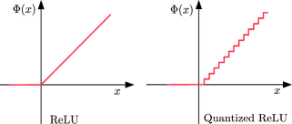
Figure 8: The expected (left) and real (right) ReLU function in low-precision networks.

In the recent work by Anitha et al. [160] a quantized complex-valued activation function was proposed. The quantized activations are also proved to be successful against the adversarial examples, see Rakin et al. [161]. Mishra et al. [162] presented wide reduced-precision networks (WRPN) to quantize activation and weights. They further found that activations take up more memory than weights. To compensate for the loss of precision due to quantization, they implemented an approach that increased the number of filters in each layer.

One well-known difficulty with quantized activation is that it causes a gradient mismatch problem, see Lin and Talthi [163]. As an example, figure 8 shows an expected and real ReLU activation function in low-precision networks. In a fixed point network, the effective activation function is a non-differentiable function. The gradient mismatch problem is the result of this discrepancy between the assumed and real activation functions.

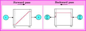
Figure 9: Schematic representation of straight through estimation (STE) derivative approximation

In [164], Bengio et al. proposed the straight through estimation (STE) derivative approximation that works well for quantized activation function. As an example, they treated the quantized ReLU activation as the identity function in the clipping range $[\alpha_{1},\alpha_{2}]$, and constant outside, which gives the unity derivative in the clipping range and zero outside. Figure 9 shows schematic representation of STE derivative approximation.

IX A quest towards an optimal activation function

Which activation function should we use? This is one of the most basic and meaningful questions that could be posed. As discussed earlier, there is no rule of thumb for choosing the optimal activation function, which strongly depends on the problem under consideration. This motivates us to ask another meaningful question: do we need an activation function that adapts itself as per the requirements, thereby avoiding the local minima by changing the loss landscape dynamically? In this way, the adaptive activation functions can beat any standard (fixed) activation function of the same type. Despite having various activation functions, the quest for having the best activation function has driven researchers to propose an activation function that is adaptive, also called adaptable, tunable, or trainable activations. In recent years, this has triggered a surge in papers on adaptive activation functions. The adaptive nature of the activation can be injected in many ways. For example, one can introduce parameters that adapt accordingly, or another way is to use ensemble activation functions from the pre-defined set of functions, which performs better than single activation. This section discusses various adaptive activation functions that perform better than their fixed counterparts.

IX-A Parametric Activation Functions

In the literature, various adaptive activation functions have been proposed. In their earlier work, Chen and Chang [42] proposed the generalized hyperbolic tangent function parameterized by two additional positive scalar values $a$ and $b$ as

$$\Phi(x)=\frac{a(1-exp(-bx))}{1+exp(-bx)},$$

where the parameters $a,b$ are initialized randomly and then adapted independently for every neuron. Vecci et al. [43] suggested a new architecture based on adaptive activation functions that use Catmull-Rom cubic splines. Trentin [44] presented empirical evidence that learning the amplitude for each neuron is preferable instead of having unit amplitude for all activation functions (either in terms of generalization error or speed of convergence). Goh et al. [45] proposed a trainable amplitude activation function. Chandra and Singh [46] proposed the activation function adapting algorithm for sigmoidal feed-forward neural network training. Eisenach et al. [48] proposed parametrically learning activation functions. Babu and Edla [49] proposed the algebraic activation functions. Ramchandran et al. [35] proposed the Swish activation function  defined as:

$$\Phi(x)=x\cdot\text{Sigmoid}(\beta\cdot x)$$

where $\beta$ is the tuning parameter. Like ReLU, Swish is unbounded above but bounded below. The Swish is shown to give faster convergence and better generalization for many test problems. In [51], Alcaide et al. proposed the E-swish activation function as

$$\Phi(x)=\beta x\cdot\text{Sigmoid}(x).$$

Mercioni et al. [165] proposed the trainable parameter based swish (p-swish) activation that can give more flexibility than the original swish activation. Ertuğrul [52] proposed the trained activation function. Choi et al. [54] proposed PArameterized Clipping acTivation (PACT) that uses an activation clipping parameter $\alpha$ that is optimized during training to find the right quantization scale. Apicella et al. [55] proposed an efficient architecture for trainable activation functions.

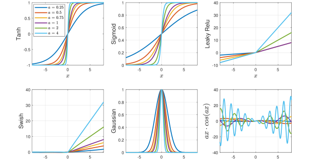
Figure 10: Adaptive activation functions for different values of adaptive parameter $a$.

Jagtap et al. [64] proposed globally adaptive activation function where they introduced a single slope parameter $a$ in the activation function as

$$\Phi(na(wx+b)),$$

where $a$ is a trainable parameter and $n\geq 1$ is pre-defined scaling factor. They initialized $na=1,\forall n\geq 1$. Figure 10 shows these globally adaptive activation functions for different values of $a$. Based on this idea, the layer-wise and neuron-wise locally adaptive activation functions were proposed [65] that can be trained faster. The main idea is to introduce trainable parameters for every hidden-layer (layer-wise adaptive activation functions) as well as for every neuron in each layer (neuron-wise adaptive activation functions). Along with these locally adaptive activations, the additional slope recovery term is added in the activation function, which is given by

$$S(a)=\begin{cases}\frac{1}{1/(D-1)\sum_{k=1}^{D-1}\text{exp}(a^{k})}&\text{For layer-wise activation}\\ \frac{1}{1/(D-1)\sum_{k=1}^{D-1}\text{exp}\left(\frac{\sum_{i=1}^{Nk}a_{i}^{k}}{N_{k}}\right)}&\text{For neuron-wise activation},\end{cases}$$

where $D$ is the depth of the network, $N_{k}$ is the number of neurons in the $k^{th}$ hidden-layer. The authors in [166] proposed self-adaptive evolutionary algorithms for searching new activation functions. The Soft-Root-Sign activation function [167] is defined as

$$\Phi(x)=\frac{x}{\frac{x}{\alpha}+\text{exp}(-x/\beta)},$$

that gives range from $\left[\frac{\alpha\beta}{\beta-\alpha\times\text{exp}},\alpha\right]$. Both $\alpha$ and $\beta$ are a pair of trainable non-negative parameters. Pratama and Kang [168] proposed trainable neural networks. Universal activation functions are proposed by Yuen et al. in [169] as

$$\Phi(x)=\text{ln}(1+e^{A(x+B)+Cx^{2}})-\text{ln}(1+e^{D(x-B)})+E,$$

where $A,B$ and $E$ controls the slope, horizontal shift and vertical shift, respectively. The parameter $D$ approximates the slope of leaky ReLU, and $C$ introduces additional degrees of freedom.

Recently, Bingham and Miikkulainen [170] discovered the parametric activation function using evolutionary search, where they used gradient descent to optimize its parameters during the learning process. In [171] Lapid and Sipper proposed a three-population, coevolutionary algorithm to evolve an activation function.

IX-A1 Adaptive family of rectifier and exponential units

In the literature, many adaptive families of rectifiers and exapnential units are proposed. This section gives a brief introduction to these activation functions.

• Parametric ReLU [37]: The parametric ReLU (PReLU) is similar to the leaky ReLU, and it is defined as

  $$\Phi(x)=\begin{cases}\alpha x&\text{for}~{}x\leq 0\\ x&\text{for}~{}x>0.\end{cases}$$

  In parametric ReLU, $\alpha$ is the learning parameter, which is learned during the optimization process. Both, leaky and parametric ReLU still face the problem of exploding gradients.

• S-Shaped ReLU : Abbreviated as SReLU [56] is defined as a combination of three linear functions, which perform a mapping $\mathbb{R}\rightarrow\mathbb{R}$ with the following formulation

  $$\Phi(x_{i})=\begin{cases}t_{i}^{r}+a_{i}^{r}(x_{i}-t_{i}^{r}),&x_{i}\geq t_{i}^{r},\\ x_{i},&t_{i}^{r}>x_{i}>t_{i}^{l},\\ t_{i}^{l}+a_{i}^{l}(x_{i}-t_{i}^{l}),&x_{i}\leq t_{i}^{l},\end{cases}$$

  where $t_{i}^{r},t_{i}^{l},a_{i}^{r},a_{i}^{l}$ are four learnable parameters. The subscript $i$ indicates that we allow SReLU to vary in different channels.

• Parametric ELU : The parametric ELU [59] was proposed in order to remove the need to specify the parameter $\alpha$, which can be learned during the training to get the proper activation shape at every CNN layer. Klambauer et al. [107] proposed Scaled exponential linear unit (SELU)

  $$\Phi(x)=\lambda\begin{cases}\alpha(\text{exp}(x)-1)&\text{for}~{}x\leq 0\\ x&\text{for}~{}x>0.\end{cases}$$

• Parametric Tanh Linear Unit (P-TELU) [172]: It is defined as

  $$\Phi(x)=\begin{cases}x&\text{for}~{}x\geq 0\\ \alpha~{}\tanh(\beta x)&\text{for}~{}x<0,\end{cases}$$

  which has range from [$-\alpha,\infty$), and both $\alpha$ and $\beta$ are trainable parameters.

• Continuously Differentiable ELU : The Continuously Differentiable ELU [60] is simply the ELU activation where the negative values have been modified to ensure that the derivative exists (and equal to 1) at $x=0$ for all values of $\alpha$. The Continuously Differentiable ELU is defined as

  $$\Phi(x)=\begin{cases}x&\text{for}~{}x\geq 0\\ \alpha(\text{exp}(x/\alpha)-1)&\text{Otherwise},\end{cases}$$

  where $\alpha$ is tunable parameter.

• Flexible ReLU [57]: The Flexible ReLU, or FReLU, is defined as

  $$\Phi(x)=ReLU(x)+b,$$

  which has a range $[b,\infty)$. The FReLU captures the negative values with a rectified point.

• Paired ReLU [58]:: The Paired ReLU is defined as

  $$\Phi(x)=[\text{max}(sx-\theta,0),\text{max}(s_{p}x-\theta_{p},0)],$$

  where $s$ and $s_{p}$ represents scale parameters, which are initialized with the values of $0.5$ and -0.5, respectively . $\theta$ and $\theta_{p}$ are a pair of trainable thresholds.

• Multiple Parametric ELU : The multiple parametric ELU [173] is given as

  $$\Phi(x)=\begin{cases}x&\text{for}~{}x>0\\ \alpha(\text{exp}(\beta x)-1)&\text{for}~{}x\leq 0.\end{cases}$$

  Here, $\beta$ is greater than zero.

• Parametric Rectified Exponential Unit : The parametric rectified EU [174] is defined as

  $$\Phi(x)=\begin{cases}\alpha x&\text{for}~{}x>0\\ \alpha x~{}\text{exp}(\beta x)&\text{for}~{}x\leq 0,\end{cases}$$

• Fast ELU : The Fast ELU [62] is given as

  $$\Phi(x)=\begin{cases}x&\text{for}~{}x>0\\ \alpha(\text{exp}(x/\text{ln}(2))-1)&\text{for}~{}x\leq 0.\end{cases}$$

  The curve trend with fast ELU is consistent with the ELU due to the fast approximation achieved, ensuring that the fast ELU does not alter the original ELU’s accuracy advantage.

• Multi-bin Trainable Linear Units (MTLU) [175]: The MTLU is given as

  $$\Phi(x)=\begin{cases}a_{0}x+b_{0}&\text{for}~{}x\leq c_{0},\\ a_{1}x+b_{1}&\text{for}~{}c_{0}<x\leq c_{1},\\ \cdots\\ a_{r}x+b_{r}&\text{for}~{}c_{r-1}<x,\end{cases}$$

  with range ($-\infty,\infty$). The MTLU considers different bins with different ranges of hyperparameters. All the parameters $a_{0},a_{1},\cdots,a_{r},b_{0},b_{1},\cdots,b_{r},c_{0},c_{1},\cdots,c_{r}$ are trainable.

• Mexican ReLU: The Mexican ReLU [176] uses Mexican hat type function and it is defined as:

  $$\Phi(x)=\text{PReLU}(x)+\sum_{i=1}^{K}c_{i}~{}\text{max}(\lambda_{i}-|x-a_{i}|,0),$$

  where $c_{i}$ are tunable parameter and $\lambda_{i},a_{i}$ are real numbers.

• Lipschitz ReLU [177]: The L* ReLU is defined as

  $$\Phi(x)=\begin{cases}\text{max}(\phi(x),0)&\text{for}~{}x\geq 0\\ \text{max}(\eta(x),0)&\text{for}~{}x<0,\end{cases}$$

  where $\phi(x)$ and $\eta(x)$ are nonlinear functions.

• Parametric Deformable ELU : First defined in [178], the parametric deformable ELU is given as

  $$\Phi(x)=\begin{cases}x&\text{for}~{}x>0\\ \alpha[(1+(1-t)x)^{1/(1-t)}-1]&\text{for}~{}x\leq 0,\end{cases}$$

  with range $(-\alpha,\infty)$.

• Elastic ELU : The Elastic ELU [63] is designed to utilize the properties of both ELU and ReLU together, and it is defined as

  $$\Phi(x)=\begin{cases}kx&\text{for}~{}x>0\\ \alpha(\text{exp}(\beta x)-1)&\text{for}~{}x\leq 0,\end{cases}$$

  where both $\alpha$ and $\beta$ are tunable parameters.

IX-B Stochastic/probabilistic adaptive activation functions

The stochastic/probabilistic approach is another way to introduce an adaptive activation function. In [66], Gulcehre et al. proposed a noisy activation function where a structured and bounded noise-like effect is added to allow the optimizer to exploit more and learn faster. This is particularly effective for the activation functions, which strongly saturate for large values of their inputs. In particular, they learn the level of injected noise in the saturated regime of the activation function. They consider the noisy activation functions of the following form:

$$\Phi_{\text{noisy}}(x)=\Phi(x)+s$$

where $s=\mu+\sigma\xi$. Here $\xi$ is an independent and identically distributed random variable drawn from generating distribution, and the parameters $\mu$ and $\sigma$ are used to generate a location scale family from $\xi$. When the unit saturates, they pin its output to the threshold value $t$, and the noise is added. The type of noise $\xi$ and the values of $\mu$ and $\sigma$, which can be chosen as functions of $x$ to allow some gradients to propagate even in the saturating regime, determine the exact behavior of the method.

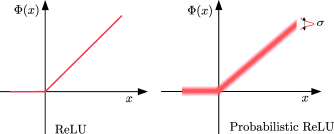
Figure 11: ReLU (left) and Probabilistic ReLU (right) activation functions.

Urban et al. [50] proposed Gaussian process-based stochastic activation functions. Based on a similar idea by Gulcehre et al. [66], Shridhar [67] proposed the probabilistic activation functions (ProbAct), which are not only trainable but also stochastic in nature, see Figure 11. The ProbAct is defined as:

$$\Phi(x)=\mu(x)+z,$$

where $\mu(x)$ is a static or learnable mean, say, $\mu(x)=max(0,x)$ for static ReLU, and the perturbation term $z=\sigma\epsilon$, where perturbation parameter $\sigma$ is a fixed or trainable value which specifies the range of stochastic perturbation and $\epsilon$ is a random value sampled from a normal distribution $\mathcal{N}(0,1)$. Because the ProbAct generalizes the ReLU activation, it has the same drawbacks as the ReLU activation.

The Rand Softplus activation function [179] models the stochaticity-adaptibility as

$$\Phi(x)=(1-\rho)~{}\text{max}(0,x)+\rho~{}\text{log}(1+e^{x}),$$

where $\rho$ is a stochastic hyperparameter.

IX-C Fractional adaptive activation functions

The fractional activation function can encapsulate many existing and state-of-the-art activation functions. In the earlier study of Ivanov [68] the fractional activation functions are presented. This is motivated by the potential benefits of having more tunable hyperparameters in a neural network and achieving different behaviors, which can be more suitable for some kinds of problems. In particular, the author used the following Mittag-Leffler types of functions:

$$E_{\alpha,\beta}(z)=\sum_{k=0}^{\infty}\frac{z^{k}}{\Gamma(\alpha k+\beta)},z\in\mathbb{C},$$

which is the class of parametric transcendental functions that generalize the exponential function. Setting $\alpha$ and $\beta$ to unity gives the Taylor series expansion of the exponential function. The authors proposed several fractional activation functions by replacing the exponential function with several standard activation functions such as tanh, sigmoid, logistic, etc.

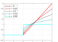
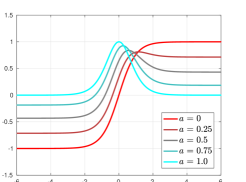
Figure 12: Fractional ReLU (left), and fractional hyperbolic tangent (right) activation functions for different values of fractional derivative $a$.

In [69], the authors proposed activation functions leveraging the fractional calculus. In particular, they used the Gamma function ($\Gamma(z)=\int_{0}^{\infty}t^{z-1}e^{-t}~{}dt$). The fractional ReLU is then defined as

$$\Phi(x)=\begin{cases}D^{a}x&x>0,\\ 0&x\leq 0,\end{cases}$$

where the fractional derivative is given by

$$D^{a}x=\frac{\Gamma(2)}{\Gamma(2-a)}x^{1-a}.$$

Similarly, the fractional derivative of hyperbolic tangent is given by

$$\Phi(x)= D^{a}tanh(x)=\lim_{h\rightarrow 0}\frac{1}{h^{a}}\sum_{n=0}^{\infty}(-1)^{n}\frac{\Gamma(a+1)~{}tanh(x-n\cdot h)}{\Gamma(n+1)\Gamma(1-n+a)}.$$

The fractional derivative produces a family of functions for different values of $a$. Figure  12 depicts the fractional ReLU (left) and fractional hyperbolic tangent (right) functions for different $a$ values. At $a=0.99$, the ReLU becomes a step function, whereas the hyperbolic tangent function ($a=0$) becomes a quadratic hyperbolic secant function.

IX-D Ensemble adaptive activation functions

An alternative approach to adaptive activation functions is to create a combination of different activation functions. The earlier work of Xu and Zhang [70] proposes an adaptive ensemble activation function consisting of sigmoid, radial basis, and sinusoid functions. In [71], Ismail et al. select the most suitable activation function as a discrete optimization problem that involves generating various combinations of functions. The proposed activation function is expressed as

$$\Phi(x)=\sum_{i=1}^{n}k_{i}~{}c_{i}~{}\psi_{i}(x),$$

where $n$ is the number of the sub-functions represented by $(\psi_{i})$ in the activation function, $c_{i}$ is an adaptive coefficient, and $k_{i}$ is a binary number.

Chen [72] used multiple activation functions for each neuron for the problems related to stochastic control. Jin et al. [56] proposed the combination of a set of linear functions with open parameters. Agostinelli et al. [47] constructed the activation functions during network training. They used the following general framework:

$$\Phi(x)=~{}\text{max}(0,x)+\sum_{p=1}^{P}a_{i}^{p}~{}\text{max}(0,-p+b_{i}^{p}),$$

where $P$ is predefined hyperparameter, $i$ is the neuron, and $a,b$ are trained variables.

Ramachandran et al [35] used a reinforcement learning controller to combine preset unary and binary functions for learning new activation functions. In [53], Qian et al. proposed adaptive activations in convolutional neural networks, where they focus on learning activation functions via combining basic activation functions in a data-driven way. In particular, they used ReLU and other variants of ReLU, such as Leaky ReLU and ELU combinations. In [180], Klabjan and Harmon show that the ensemble activation function can be created by choosing the suitable activation functions from the predefined set $A=\{A_{1},A_{2},\cdots,A_{m}\}$. Here, the activations are combined together to get the best performance out of the neural networks. A similar approach was used by Nandi et al. in [181], where an ensemble of activation functions is used to improve the performance of the network. In [55] , Apicella et al. proposed to modify a feed-forward neural network by adding Variable Activation Functions (VAF) in terms of one-hidden layer subnetworks. The previously discussed Mexican ReLU [176] also comes under the category of ensemble activation functions.

A polynomial activation function was proposed in [182] where they built the activation function over powers of the activation. They used

$$\Phi(x)=\sum_{i=0}^{P}\alpha_{i}x^{i},$$

where $P$ is a hyper-parameter. Because a polynomial of degree $P$ can pass through all $P+1$ points exactly, this polynomial activation function can theoretically approximate any smooth function. The main disadvantage was the global influence of coefficient $\alpha_{i}$, which causes the function’s output to grow excessively large. Similarly, Scardapane et al. [183] proposed the kernel-based non-parametric activation function. In particular, they model each activation function in terms of a kernel expansion over a finite number of terms as

$$\Phi(x)=\sum_{i=1}^{D}\alpha_{i}\kappa(x,d_{i}),$$

where $\{\alpha_{i}\}_{i=1}^{D}$ are the mixing coefficients, $\{d_{i}\}_{i=1}^{D}$ are the called the dictionary elements, and $\kappa(·,·):\mathbb{R}\times\mathbb{R}\rightarrow\mathbb{R}$ is a one-dimensional kernel function. Further, this idea was extended with a multi-kernel approach in [184]. On similar grounds, the adaptive blending units [185] were proposed by Sütfeld et al. to combine a set of functions in a linear way. In [186], Basirat and Roth presented a genetic algorithm based learning of activation functions where the hybrid crossover of various operators results in a hybrid activation function.

References	Parametric	Ensemble	Stochastic/	Fractional	Complex-Valued	Quantized
			Probabilistic
Chen and Chang [42], Vecci [43], Trentin [44]
Goh [45], Chandra and Singh [46], Shah et al. [59],
Jin et al.[56], Shah [59], Jin [56]	✓	✗	✗	✗	✗	✗
He et al. [37], Barron [60], Duggal and Gupta [172]
Li et al. [173], Tang et al.[58], Qiu et al. [57]
Grelsson and Felsberg [61], Ying et al. [174], Qiumei et al. [62]
Gu et al. [175], Goyal et al. [187], Jagtap et al. [64, 65]
Basirat and Roth [177], Cheng et al. [178], Kim et al. [63]
Piazza et al. [182], Agostinelli et al. [47] Jagtap et al. [73]	✓	✓	✗	✗	✗	✗
Scardapane et al. [183]
Gulcehre et al. [66], Shridhar et al. [67], Urban et al.[50]	✓	✗	✓	✗	✗	✗
Zamora et al. [69], Ivanov et al. [68]	✓	✗	✗	✓	✗	✗
Xu and Zhang [70], Ismail et al. [71]
Ramchandran et al. [35], Klabjan and Harmon [180]	✗	✓	✗	✗	✗	✗
Sütfeld et al. [185], Basirat and Roth [186]
Nanni et al [188]	✗	✓	✓	✗	✗	✗
Choi et al. [54], Rakin et al. [161]	✓	✗	✗	✗	✗	✓

TABLE II: Adaptive activation functions under various settings.

In recent years, Nanni et al. [188] proposed stochastic selection of activation layers for convolutional neural networks. In [73] Jagtap et al. proposed the Kroneker Neural Networks (KNN), which is a general framework for adaptive activation functions that can generalize a class of existing feed-forward neural networks that utilize adaptive activation functions. In particular, the output of KNN is given as

$$u^{\mathcal{K}}_{\Theta_{\mathcal{K}}}(x)=\sum_{i=1}^{N}c_{i}\left[\sum_{k=1}^{K}\alpha_{k}^{i}\Phi_{k}(\omega_{k}^{i}(w_{i}^{T}x+b_{i}))\right],$$

where the network parameters are: $\Theta_{\mathcal{K}}=\{c_{i},w_{i},b_{i}\}\cup\{\alpha_{k}^{i},\omega_{k}^{i}\}$ for $i=1,\cdots,N$ and $k=1,\cdots,K$. Different classes of adaptive activation functions are produced by varying these parameters and the hyperparameter $K$. For example,

• If $K=1$, $\omega^{i}=\alpha^{i}=1$ for all $i$, the Kronecker network becomes a standard feed-forward network.

• If $K=1$, the Kronecker network becomes a feed-forward neural network with layer-wise locally adaptive activation functions [64, 65].

• If $K=2$, $\omega^{i}_{1}=1$, $\omega^{i}_{2}=\omega_{2}$ for all $i$, $\Phi_{1}(x)=\max\{x,0\}$, and $\Phi_{2}(x)=\max\{-x,0\}$, the Kronecker network becomes a feed-forward network with Parametric ReLU activation [37].

• If $K=2$, $\omega^{i}_{2}=\omega$ for all $i$, $\Phi_{1}(x)=\max\{x,0\}$, and $\Phi_{2}(x)=(e^{x}-1)\cdot\mathbb{I}_{x\leq 0}(x)$, the Kronecker network becomes a feed-forward network with Exponential Linear Unit (ELU) activation [39] if $\omega^{i}_{1}=1$ for all $i$, and becomes a feed-forward network with Scaled Exponential Linear Unit (SELU) activation [107] if $\omega^{i}_{1}=\omega^{\prime}$ for all $i$.

• If $\omega^{i}=1$ for all $i$ and $\Phi_{k}(x)=x^{k-1}$ for all $k$, the Kronecker network becomes a feed-forward neural network with self-learnable activation functions (SLAF) [187]. Similarly, a FNN with smooth adaptive activation function [189] can be represented by a Kronecker network.

In [190] Nanni et al. used the ensembling method to compare different convolutional neural network activation functions. In particular, they used the set of twenty activation functions.

Every type of adaptive activation that has been discussed in this section has pros and cons of its own. Table II shows the adaptive activation function referenced under various settings.

X Performance of some fixed and adaptive activation functions for classification tasks

This section discusses the performance of different activation functions for classification tasks. In particular, we used MNIST [88], CIFAR-10, and CIFAR-100 [191] data sets for the same. The MNIST database of handwritten digits contains the training set of 60k samples, while the test set contains 10k examples. The CIFAR-10 data set contains 50k training and 10k testing images from 10 object categories, whereas the CIFAR-100 data set contains 50k training and 10k testing images from 100 object categories. In particular, for comparison, we chose some fixed as well as some adaptive activation functions that have been discussed previously.

	MNIST	CIFAR-10	CIFAR-100
Sigmoid	97.9 [192]	89.43 $\pm$ 0.51 (M), 85.42 $\pm$ 0.47 (V)	61.64 $\pm$ 0.56 (M), 59.25 $\pm$ 0.45 (V)
Tanh	98.21[48]	88.19 $\pm$ 1.21 (M), 87.53 $\pm$ 0.67 (V)	57.06 $\pm$ 2.03 (M), 62.32 $\pm$ 0.82 (V)
Swish	99.75 $\pm$ 0.11 (M), 99.45 $\pm$ 0.26 (V)	95.5 [35]	83.9 [35]
ReLU	99.1 [55], 99.15 [183], 99.53 [56]	95.3 [35], 94.59 [193], 92.27 [56]	83.7 [35], 75.45 [193], 67.25 [56]
Leaky ReLU	98.2 [192],99.58 [56]	95.6[35], 92.32 [53]	83.3[35], 67.3[56]
ELU	98.3 [192]	94.4 [35], 94.01 [193]	80.6 [35], 74.92[193]
PReLU	99.64 $\pm$ 0.24 (M), 99.18 $\pm$ 0.17 (V)	92.46 $\pm$ 0.44 (M), 91.63 $\pm$ 0.31 (V)	69.46 $\pm$ 0.74 (M), 66.53$\pm$ 0.69 (V)
SELU	98.42 $\pm$ 0.53 (M), 99.02 $\pm$ 0.37(V)	93.52 $\pm$ 0.63 (M), 90.53 $\pm$ 0.36 (V)	70.42 $\pm$ 0.75 (M), 68.02$\pm$ 1.29 (V)
RReLU	99.23 $\pm$ 0.53 (M), 99.63 $\pm$ 0.6 (V)	90.52 $\pm$ 2.14 (M), 90.18 $\pm$ 0.91 (V)	68.62 $\pm$ 0.42 (M), 65.32 $\pm$ 1.74 (V)
GELU	99.72 $\pm$ 0.35 (M), 99.26 $\pm$ 0.42 (V)	94.76 $\pm$ 0.55 (M), 92.67 $\pm$ 0.89 (V)	71.73 $\pm$ 1.09 (M), 69.61 $\pm$ 1.53 (V)
CELU	99.36 $\pm$ 0.68 (M), 99.37 $\pm$ 0.38 (V)	90.26 $\pm$ 0.12 (M), 90.37 $\pm$ 0.23 (V)	70.26 $\pm$ 1.53 (M), 68.35 $\pm$ 0.87 (V)
Softplus	98.69 $\pm$ 0.5 (M), 97.36 $\pm$ 0.77 (V)	94.9 [35]	83.7 [35]
Mish	97.9 [192]	90.26 $\pm$ 0.52 (M), 86.05 $\pm$ 0.76 (V)	68.53 $\pm$ 0.86 (M), 67.03 $\pm$ 1.39 (V)
Maxout	99.55 [127]	90.62 [127]	61.43 [127]
SRS	98.04 $\pm$ 0.97 (M), 98.06 $\pm$ 0.84 (V)	89.35 $\pm$ 0.85 (M), 87.26 $\pm$ 1.38 (V)	65.20 $\pm$ 1.53 (M), 63.65 $\pm$ 2.63 (V)
Ensemble ([180])	99.40 [180]	85.05 $\pm$ 0.28 (M), 84.96 $\pm$ 0.87 (V)	74.20 [180]
LiSHT	98.74 $\pm$ 0.17 (M), 98.32 $\pm$ 0.19 (V)	90.78 $\pm$ 0.43 (M),87.74 $\pm$ 0.36 (V)	56.35 $\pm$ 0.58 (M), 58.74 $\pm$ 0.99 (V)
Sine	99.10 $\pm$ 0.82 (M), 98.63 $\pm$ 0.27 (V)	91.64 $\pm$ 0.36 (M), 90.59 $\pm$ 0.88 (V)	80.98 $\pm$ 0.81 (M), 78.42 $\pm$ 0.67 (V)
GCU ([126])	97.80 $\pm$ 1.02 (M), 90.73 $\pm$ 0.87 (V)	90.24 $\pm$ 1.96 (M), 89.56 $\pm$ 0.18 (V)	77.46 $\pm$ 2.91 (M), 76.46 $\pm$ 1.61 (V)
Gaussian	98.60 $\pm$ 2.22 (M), 96.43 $\pm$ 2.57 (V)	90.64 $\pm$ 2.76 (M), 89.59 $\pm$ 0.28 (V)	76.96 $\pm$ 0.41 (M), 74.62 $\pm$ 2.69 (V)
Adaptive sine	99.56 $\pm$ 0.56 (M), 98.76 $\pm$ 0.12 (V)	92.64 $\pm$ 0.36 (M), 92.72 $\pm$ 0.37 (V)	81.15 $\pm$ 0.81 (M), 78.73 $\pm$ 0.64 (V)
Adaptive tanh	99.52 $\pm$ 0.36 (M), 99.57 $\pm$ 0.20 (V)	91.14 $\pm$ 0.45 (M), 90.52 $\pm$ 0.82 (V)	83.82 $\pm$ 0.83 (M), 76.21 $\pm$ 1.95 (V)
Adaptive ReLU	99.75 $\pm$ 0.25 (M), 98.43 $\pm$ 0.32 (V)	96.89 $\pm$ 0.93 (M), 94.77 $\pm$ 1.16 (V)	$\mathbf{84.58\pm 0.42}$ (M), 80.30 $\pm$ 0.60 (V)
Rowdy Sine	99.74 $\pm$ 0.29 (M), 99.24 $\pm$ 0.43 (V)	93.87 $\pm$ 0.78 (M), 92.82 $\pm$ 0.82 (V)	83.73 $\pm$ 0.83 (M), 82.14 $\pm$ 0.13 (V)
Rowdy tanh	99.45 $\pm$ 0.93 (M), 98.65 $\pm$ 0.57 (V)	93.78 $\pm$ 0.13 (M), 93.26 $\pm$ 0.42 (V)	82.34 $\pm$ 1.01 (M), 80.97 $\pm$ 0.32 (V)
Rowdy ReLU	99.43 $\pm$ 0.68 (M), 98.23 $\pm$ 0.25 (V)	$\mathbf{95.57\pm 0.84}$ (M), 94.47 $\pm$ 0.92 (V)	$82.75\pm 0.51$ (M), 79.41 $\pm$ 0.75 (V)
Rowdy ELU	$\mathbf{99.79\pm 0.08}$ (M), 99.06 $\pm$ 1.07 (V)	95.45 $\pm$ 0.92 (M), 93.27 $\pm$ 0.13 (V)	84.29 $\pm$ 0.13 (M), 82.40 $\pm$ 0.81 (V)

TABLE III: Accuracy comparison of different activation functions for MNIST, CIFAR-10, and CIFAR-100 data sets. Here, we report the best accuracy from the literature without considering the architecture used to perform the experiments. Also, we used MobileNet [194] (denoted by M) and VGG16 [195] (denoted by V) architectures with different activation functions, where we report the mean and standard deviations of 10 different realizations. The Adaptive and Rowdy (with $K=3$) refers [64] and [73], respectively. The best results are highlighted in bold.

In this work, we report the best accuracy from the literature without considering the architecture used to perform the experiments. We also conducted a performance comparison of two models, namely, MobileNet [194] and VGG16 [195]. Both MobileNet and VGG16 have a convolution neural net (CNN) architecture. The MobileNet is a lightweight deep neural network with better classification accuracy and fewer parameters, whereas the VGG16 has 16 deep layers. In both cases, the learning rate is 1e-4, and the batch sizes for MNIST, CIFAR-10 and CIFAR-100 are 64, 128, and 64, respectively. During training and testing, data normalization is performed. The Adam [196] optimizer is employed with a cross-entropy loss function. All the experiments are computed using a desktop computer system having 16 GB of RAM with an Nvidia GPU Card, and performed in the Pytorch [197] environment, which is a popular machine learning library.

Table III gives the accuracy comparison of different activation functions for all the three data sets, where we have given the mean and standard deviation of accuracy for 10 different realizations. For MNIST, almost all activation functions perform well. It can be observed that the Swish, ReLU, Leaky ReLU, ELU, and Sine activation functions work well for the CIFAR-10 and CIFAR-100 data sets. Furthermore, in all three data sets, the adaptive and rowdy activation functions outperform.

XI Activation functions for physics-informed machine learning

In recent years, physics-based machine learning (PIML) [20] algorithms for scientific calculations have been revived at a considerably faster speed owing to the success of automatic differentiation (AD) [198]. These methods can solve not only the forward problems but also the notoriously difficult inverse problems governed by almost any type of differential equation. Various physics-informed machine learning algorithms have been proposed that can seamlessly incorporate governing physical laws into a machine learning framework. The SINDy framework [199] for analyzing dynamical systems, physics-informed machine learning for modeling turbulence [200], physics-guided machine learning framework [201], the Neural ODE [202], and most recently physics-informed neural networks (PINNs) [203] are just a few examples of the many physics-informed machine learning algorithms that have been proposed and successfully used for solving problems from computational science and engineering fields.

Most of our previous discussion about activation function was centered around various classification problems in the computer science community. In this section, we focus on the activation functions for the PIML framework. Apart from the accurate and efficient AD algorithm, PIML methods also need tailored activation functions where the output of the network not only satisfies the given data but also satisfies the governing physical laws in the form of differential equations where various spatio-temporal derivative terms are involved. In this work, we are using PINNs for our investigation. PINN is a very efficient method for solving both forward and ill-posed inverse differential equations involving sparse and multi-fidelity data. The main feature of the PINN is that it can seamlessly incorporate all the information, like governing equation, experimental data, initial/boundary conditions, etc., into the loss function, thereby recasting the original PDE problem into an optimization problem. PINNs achieved remarkable success in many applications in science and engineering; see [204, 205, 206, 207, 208, 209, 210, 211, 212], and the references therein for more details. The first comprehensive theoretical analysis of PINNs for a prototypical nonlinear PDE, the Navier-Stokes equations, has been presented in [213].

XI-A Differentiability

Differentiability is an important property of the activation function. The activation function must be differentiable everywhere. Consider the example of one-dimensional Laplace equation with forcing $f$ as

$$\frac{d^{2}}{dx^{2}}u=-f, ~{}x\subset\mathbb{R}.$$

Here we use a one-hidden-layer neural network with a single neuron, see figure 13.

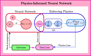
Figure 13: Left part: One-hidden layer, single neuron, feed-forward neural network, and right part: physics-informed part where neural network’s output is forced to satisfy the governing physical laws. In particular, the automatic differentiation (AD) is employed to find the derivatives present in the governing differential equation.

The network’s input is the independent variable $x$, and its output is $u_{NN}\approx u(x)$. The network output $u_{NN}$ satisfies both data as well as physics, as shown in the figure. The loss function is given as

$$\mathcal{L}(\Theta)=\sum_{j=1}^{N_{u}}|u^{j}_{NN}(\Theta)-u_{\text{data}}|^{2}+\sum_{j=1}^{N_{f}}|\mathcal{F}^{j}(\Theta)|^{2},$$

where the first term on RHS is the data mismatch loss where $N_{u}$ are the number of data points, and the second term is the residual of the ODE given as $\mathcal{F}\triangleq\frac{d^{2}}{dx^{2}}(u_{NN})-f$ with $N_{f}$ collocation points. The symbol $\Theta$ represents all the tunable parameters in the networks, such as weights, biases, etc. Let $\Phi$ be the activation function that is applied before passing the output of the neuron. Then, the network output can be given as

$$u_{NN}=\Phi(w\cdot x+b).$$

The network output $u_{NN}$ not only satisfies the given data obtained from the boundary conditions or the experimental results, but also satisfies the physical laws (ODE residue), as shown by the right-hand side blue box where the AD is employed to differentiate the network’s output. It can be seen that the activation function plays an important role in order to correctly enforce the physical laws. In this case we required the value of

$$\frac{d^{2}}{dx^{2}}(u_{NN})= \frac{d^{2}}{dx^{2}}\Phi(w\cdot x+b).$$

This requirement imposes several restrictions on the activation functions, especially high-order of continuity. In particular, activation functions such as step function, ReLU, and leaky ReLU are not good candidates for solving such problems for the obvious reason of the non-existence of their derivatives in particular locations.

The most commonly used activation function that has been successfully employed in physics-informed machine learning frameworks is the hyperbolic tangent function. In recent years, sinusoidal activation functions have been shown to be beneficial for certain PDEs [64]. In this section, we systematically compare the performances of different activation functions for the following three partial differential equations where the order of derivative increases from the first to the last case.

Case 1 : Linear Convection Equation (LCE) is a hyperbolic conservation laws given as

$$u_{t}+cu_{x}=0,~{}x\in[0,2],t>0,$$

where $c=1.0$ is the wave speed. If the initial profile is $u(0,x)=u_{0}(x)$, then the exact solution is $u(t,x)=u_{0}(x-ct)$. The initial condition is a square pulse, which moves in space from left to right without changing its shape.

Case 2 : Viscous Burgers Equation is given as

$$u_{t}+uu_{x}=\nu u_{xx},~{}x\in[-1,1],t>0,$$

where $c=1.0$ is the wave speed. $u(0,x)=-\sin(\pi x)$ is the initial profile, and the exact solution is obtained using spectral methods. The viscosity coefficient $\nu=0.01/\pi$. Due to the dominant nonlinear convection term, the viscous Burgers gives a high gradient solution.

Case 3 : The Boussinesq Equation with Dirichlet boundary and initial conditions is given by

$$u_{tt}-u_{xx}-u_{xxxx}-3(u^{2})_{xx}=0,~{}x\in[-20,20],t\in[-5,5],$$

with $u(x,-5)=u_{0}(x),$ is the initial condition. The exact solution is assumed to be of the form

$$u(x,t)=\frac{1}{2}\text{sech}^{2}\left(\frac{x+t\sqrt{2}}{2}\right).$$

	$\#$ Layers	$\#$ Neurons	$\#$ Residual Pts.	$\#$ Data Pts.	Learning rate
Case 1	4	30	7000	150	4e-04
Case 2	6	30	8000	200	1e-04
Case 3	6	40	14000	300	1e-04

TABLE IV: The hyperparameters used for three cases.

	Case 1	Case 2	Case 3
Fixed Sine	$\mathbf{3.545e-03\pm 4.581e-04}$	$5.894e-03\pm 5.436e-04$	$\mathbf{6.490e-03\pm 3.846e-04}$
Fixed GCU	$4.553e-03\pm 7.633e-04$	$8.225e-03\pm 3.736e-04$	$8.095e-03\pm 7.757e-04$
Fixed Sigmoid	$2.643e-02\pm 7.536e-03$	$1.967e-01\pm 6.382e-02$	$3.646e-01\pm 6.547e-02$
Fixed Tanh	$4.989e-03\pm 5.938e-04$	$\mathbf{4.001e-03\pm 4.504e-04}$	$6.546e-03\pm 5.007e-04$
Fixed Swish	$6.224e-03\pm 5.995e-04$	$7.782e-03\pm 6.648e-04$	$7.648e-03\pm 6.864e-04$
Fixed ELU ($\mathbf{\alpha=1}$)	$1.549e-02\pm 7.588e-03$	-	-
Adaptive Sine	$2.255e-03\pm 5.627e-04$	$3.052e-03\pm 4.368e-04$	$\mathbf{1.370e-03\pm 4.526e-04}$
Adaptive GCU	$3.908e-03\pm 4.683e-04$	$2.126e-03\pm 3.877e-04$	$1.875e-03\pm 5.117e-04$
Adaptive Sigmoid	$1.052e-02\pm 5.442e-03$	$1.011e-01\pm 4.637e-02$	$1.992e-01\pm 2.621e-02$
Adaptive Tanh	$\mathbf{1.927e-03\pm 4.821e-04}$	$\mathbf{1.731e-03\pm 6.890e-04}$	$2.552e-03\pm 6.909e-04$
Adaptive Swish	$4.652e-03\pm 7.627e-04$	$2.931e-03\pm 7.526e-04$	$3.526e-03\pm 5.267e-04$
Adaptive ELU ($\mathbf{\alpha=1}$)	$1.215e-02\pm 5.007e-03$	-	-
Rowdy Sine	$\mathbf{9.526e-04\pm 8.226e-05}$	$1.525e-03\pm 3.526e-04$	$\mathbf{8.356e-04\pm 5.556e-04}$
Rowdy GCU	$1.262e-03\pm 2.526e-04$	$\mathbf{1.206e-03\pm 4.524e-04}$	$1.523e-03\pm 9.442e-04$
Rowdy Sigmoid	$6.326e-03\pm 9.767e-04$	$6.257e-02\pm 8.116e-03$	$6.362e-02\pm 5.562e-03$
Rowdy Tanh	$1.637e-03\pm 3.960e-04$	$1.902e-03\pm 6.362e-04$	$1.049e-03\pm 4.257e-04$
Rowdy Swish	$1.986e-03\pm 6.398e-04$	$2.526e-03\pm 5.257e-04$	$1.018e-03\pm 3.466e-04$
Rowdy ELU ($\mathbf{\alpha=1}$)	$3.499e-03\pm 4.810e-03$	-	-

TABLE V: Mean and standard deviation of relative $L_{2}$ errors for three cases using different fixed and adaptive activation functions. The Adaptive and Rowdy (with $K=5$) refers [64] and [73], respectively. The column-wise best results are highlighted in bold for fixed, adaptive and Rowdy activation functions.

Table IV shows all the hyperparameters that have been chosen for three different test cases. The number of data points represents both boundary as well as initial data. We used the first 10,000 iterations of the Adam [196] optimizer followed by the L-BFGS [214] optimizer till convergence. Table V displays the mean and standard deviation of the relative $L_{2}$ error for ten different realizations. It can be seen that sine, tanh, and Swish perform well in all cases, where as ELU’s performance is poor in the first case. ELU can not be used for cases 2 and 3, as its higher order derivative does not exist. The sigmoid performs poorly, especially for PDEs involving high-order derivatives. This is obvious because higher order sigmoid derivatives have low amplitude, as shown in Figure 14. Moreover, both adaptive and rowdy activations perform well compared to their fixed counterparts. The column-wise best performance of the activation function is shown using the bold symbols.

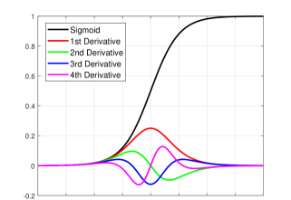
Figure 14: The Sigmoid and its derivatives.

Although the fixed activation function gives better predictive accuracy, it is well known that the adaptive activation functions perform better than their fixed counterparts; see, for example, [64, 65].

XI-B Range

The range of the activation function is another important aspect that needs further discussion. The field variable’s range is occasionally known a priori when using the PIML framework to solve PDEs. For instance, the fluid’s density will always be positive while simulating fluid flows (if there is no vacuum state present in the flow). The selection of an activation function for the output layer depends strongly on this information. In the fluid example, activation can be used to produce only positive values by discarding all negative ones. This effective selection of activation functions and incorporation of prior knowledge about the field variables has an immediate impact on the convergence of network training.

XI-C Performance comparison using different machine learning libraries

Several machine learning libraries, such as TensorFlow [215], PyTorch [197], and JAX [216] can be used to efficiently implement PINNs. Python is a more practical language to use for PINNs because it is the most popular programming language for machine learning, hence the majority of these packages are developed in Python. Deep learning libraries such as PyTorch and Tensorflow offer high-level APIs for modern deep learning techniques. In contrast, the JAX library for arbitrary differentiable programming is more functionally oriented. JAX is a new high-performance machine learning library that combines Autograd [217] and Accelerated Linear Algebra (XLA) [216]. The Autograd implementation in JAX enables automatic differentiation between native Python and NumPy routines. In addition to forward-mode differentiation, the Autograd engine in JAX also enables reverse-mode differentiation, and the two can be combined in any order. To get the benefits of static compilation and interpretation, just-in-time (JIT) compilation is used. For this, JAX also takes advantage of XLA to enhance the functionality of the compiled code.

In this work, we compare various activation functions for accurately evaluating the derivatives in the governing equations using TensorFlow (TF2), PyTorch, and JAX (with JIT) libraries.

	TensorFlow	Pytorch	JAX
Fixed Sine	$6.490e-03\pm 3.846e-04$	$7.086e-03\pm 4.637e-04$	$\mathbf{1.090e-03\pm 2.860e-04}$
Fixed GCU	$5.125e-03\pm 6.463e-04$	$5.998e-03\pm 3.657e-04$	$\mathbf{1.346e-03\pm 4.647e-04}$
Fixed Sigmoid	$3.646e-01\pm 6.547e-02$	$4.683e-01\pm 5.483e-02$	$\mathbf{8.638e-02\pm 8.956e-03}$
Fixed Tanh	$6.546e-03\pm 5.007e-04$	$7.859e-03\pm 8.750e-04$	$\mathbf{8.599e-04\pm 9.907e-05}$
Fixed Swish	$7.648e-03\pm 6.864e-04$	$5.011e-03\pm 7.486e-04$	$\mathbf{9.053e-04\pm 8.082e-05}$
Adaptive Sine	$1.370e-03\pm 4.526e-04$	$3.372e-03\pm 3.163e-04$	$\mathbf{7.440e-04\pm 6.060e-05}$
Adaptive GCU	$3.986e-03\pm 5.647e-04$	$2.575e-03\pm 5.775e-04$	$\mathbf{9.221e-04\pm 8.836e-05}$
Adaptive Sigmoid	$1.992e-01\pm 2.621e-02$	$7.683e-02\pm 9.083e-03$	$\mathbf{4.638e-03\pm 8.994e-03}$
Adaptive Tanh	$2.552e-03\pm 6.909e-04$	$2.157e-03\pm 7.111e-04$	$\mathbf{5.489e-04\pm 6.995e-05}$
Adaptive Swish	$3.526e-03\pm 5.267e-04$	$1.738e-03\pm 4.738e-04$	$\mathbf{6.053e-04\pm 7.072e-05}$
Rowdy Sine	$8.356e-04\pm 5.556e-04$	$1.098e-03\pm 3.226e-04$	$\mathbf{2.578e-04\pm 2.860e-04}$
Rowdy GCU	$1.003e-03\pm 1.858e-04$	$2.012e-03\pm 4.676e-04$	$\mathbf{3.792e-04\pm 3.094e-04}$
Rowdy Sigmoid	$6.362e-02\pm 5.562e-03$	$2.563e-02\pm 5.256e-03$	$\mathbf{3.678e-03\pm 4.976e-04}$
Rowdy Tanh	$1.049e-03\pm 4.257e-04$	$8.861e-04\pm 7.850e-05$	$\mathbf{3.798e-04\pm 8.857e-05}$
Rowdy Swish	$1.018e-03\pm 3.466e-04$	$9.061e-04\pm 8.659e-05$	$\mathbf{2.748e-04\pm 6.092e-05}$

TABLE VI: Clean Data: Performance comparison of the predictive accuracy of the solution of the Boussinesq equation using different ML libraries. We used different fixed and adaptive activation functions to compare the performance. The row-wise best results are highlighted in bold for all the activation functions.

	TensorFlow	Pytorch	JAX
Fixed Sine	$1.037e-02\pm 4.537e-03$	$4.073e-02\pm 7.411e-03$	$\mathbf{7.570e-03\pm 5.950e-04}$
Fixed GCU	$5.624e-02\pm 7.378e-03$	$2.457e-02\pm 3.952e-03$	$\mathbf{8.866e-03\pm 4.273e-04}$
Fixed Sigmoid	$5.286e-01\pm 6.077e-02$	$5.983e-01\pm 7.483e-02$	$\mathbf{2.196e-01\pm 2.956e-02}$
Fixed Tanh	$9.820e-03\pm 1.607e-03$	$3.314e-02\pm 7.525e-03$	$\mathbf{7.021e-03\pm 9.907e-04}$
Fixed Swish	$9.964e-03\pm 2.726e-03$	$8.521e-02\pm 9.627e-03$	$\mathbf{8.045e-03\pm 8.082e-04}$
Adaptive Sine	$9.362e-03\pm 1.008e-03$	$1.257e-02\pm 7.004e-03$	$\mathbf{4.526e-03\pm 1.539e-03}$
Adaptive GCU	$8.053e-03\pm 3.358e-04$	$2.057e-02\pm 1.641e-03$	$\mathbf{5.647e-03\pm 5.778e-04}$
Adaptive Sigmoid	$2.637e-01\pm 5.821e-02$	$2.376e-01\pm 5.222e-02$	$\mathbf{7.001e-02\pm 4.526e-03}$
Adaptive Tanh	$8.003e-03\pm 3.027e-03$	$1.078e-02\pm 5.373e-03$	$\mathbf{7.352e-03\pm 7.087e-04}$
Adaptive Swish	$6.904e-03\pm 8.637e-04$	$3.637e-02\pm 6.992e-03$	$\mathbf{3.565e-03\pm 9.227e-04}$
Rowdy Sine	$6.226e-03\pm 8.267e-04$	$8.274e-03\pm 1.860e-03$	$\mathbf{2.523e-03\pm 1.436e-03}$
Rowdy GCU	$7.644e-03\pm 6.001e-04$	$5.436e-03\pm 9.570e-04$	$\mathbf{3.444e-03\pm 8.653e-04}$
Rowdy Sigmoid	$8.286e-02\pm 6.137e-03$	$8.364e-02\pm 8.003e-03$	$\mathbf{3.842e-02\pm 2.956e-02}$
Rowdy Tanh	$2.536e-03\pm 8.847e-04$	$8.000e-03\pm 6.141e-04$	$\mathbf{9.091e-04\pm 1.737e-04}$
Rowdy Swish	$3.663e-03\pm 6.756e-04$	$9.032e-03\pm 2.367e-03$	$\mathbf{8.255e-04\pm 3.530e-04}$

TABLE VII: Noisy data (5% random Gaussian noise): Performance comparison of the predictive accuracy of the solution of the Boussinesq equation using different ML libraries. We used different fixed and adaptive activation functions to compare the performance. The row-wise best results are highlighted in bold for all the activation functions.

For this reason, we consider the Boussinesq equation because of the presence of a fourth-order derivative term. Moreover, we used the same hyperparameters defined earlier to solve the Boussinesq equation. The Adam optimizer is used for the first 10,000 iterations, followed by the L-BFGS optimizer till convergence. The mean and standard deviation of relative $L_{2}$ error for ten different realizations are shown in Table VI, which compares the predictive accuracy of the solution using TensorFlow, PyTorch, and JAX libraries for clean data. It can be seen that compared to TensorFlow and Pytorch, JAX improves the predictive accuracy in all cases, including fixed, adaptive, and Rowdy activation functions. We also compare the predictive accuracy of the solution for the noisy data. In particular, we have added 5 % random Gaussian noise to the initial and boundary data sets to achieve this. Table VII shows this comparison, where it can be seen that the predictive accuracy degrades by almost an order of magnitude in all cases. Again, in all cases, compared to the Tensorflow and Pytorch libraries, JAX offers a substantial increase in accuracy (about an order of magnitude) in the solution of PDEs.

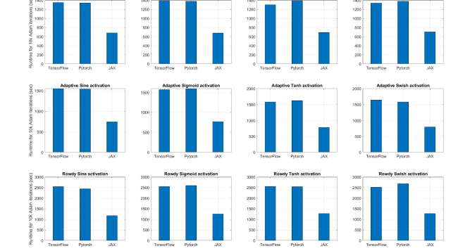
Figure 15: TensorFlow, Pytorch, and JAX run-time evaluations for the first 10,000 Adam iterations of the Boussinesq equation with clean data. The top row consists of fixed activations, the middle row consists of adaptive activations, and the bottom row consists of Rowdy activations with $(K=2)$.

The runtime comparison of TensorFlow, Pytorch, and JAX for the first 10,000 Adam iterations of the Boussinesq equation with clean data is shown in Figure 15. The top row consists of fixed activations, the middle row consists of adaptive activations, and the bottom row consists of Rowdy activations with $(K=2)$. It can be observed that adaptive activation increases the overall cost by 8-10% compared to fixed activations. In the case of Rowdy activations, the cost increment is around 75-80%. One remedy to overcome the cost associated with Rowdy activations is to use the transfer learning strategy discussed [73]. In all cases, JAX (with JIT) is computationally much more efficient than the TensorFlow (TF2) and Pytorch libraries.

Next, we compare different activation functions for function approximation using only data points.

	Function Approximation	Helmholtz Equation (JAX)
Sine	$1.865e-1\pm 4.463e-2$	$\mathbf{1.032e-1\pm 5.645e-2}$
GCU	$2.106e-1\pm 5.052e-2$	$1.564e-1\pm 4.995e-2$
Sigmoid	$3.402e-1\pm 4.052e-2$	$4.958e-1\pm 7.845e-2$
Tanh	$1.859e-1\pm 7.982e-2$	$1.378e-1\pm 4.284e-2$
Swish	$\mathbf{8.327e-2\pm 7.432e-2}$	$2.734e-1\pm 2.115e-2$
ReLU	$1.742e-1\pm 8.055e-2$	-
Leaky ReLU	$8.963e-1\pm 9.012e-2$	-
ELU	$3.737e-1\pm 9.012e-2$	-
Adaptive Sine	$6.673e-2\pm 5.715e-3$	$8.553e-2\pm 7.473e-3$
Adaptive GCU	$4.709e-2\pm 8.055e-3$	$9.042e-2\pm 6.647e-3$
Adaptive Sigmoid	$5.245e-2\pm 4.035e-3$	$9.537e-2\pm 4.365e-3$
Adaptive Tanh	$\mathbf{3.637e-2\pm 7.982e-3}$	$\mathbf{8.257e-2\pm 5.737e-3}$
Adaptive Swish	$4.626e-2\pm 8.463e-3$	$9.952e-2\pm 9.115e-3$
Adaptive ReLU	$8.436e-2\pm 1.687e-3$	-
Adaptive Leaky ReLU	$6.362e-2\pm 4.239e-3$	-
Adaptive ELU	$7.362e-2\pm 8.603e-3$	-
Rowdy Sine	$6.478e-3\pm 8.858e-4$	$\mathbf{4.872e-2\pm 5.486e-3}$
Rowdy GCU	$7.997e-3\pm 5.857e-4$	$7.473e-2\pm 4.778e-3$
Rowdy Sigmoid	$5.245e-3\pm 4.035e-4$	$6.462e-2\pm 2.084e-3$
Rowdy Tanh	$4.971e-3\pm 3.745e-4$	$5.137e-2\pm 5.677e-3$
Rowdy Swish	$\mathbf{3.245e-3\pm 4.035e-4}$	$6.932e-2\pm 6.354e-3$
Rowdy ReLU	$7.985e-3\pm 1.031e-3$	-
Rowdy Leaky ReLU	$5.342e-3\pm 8.259e-4$	-
Rowdy ELU	$6.362e-3\pm 9.534e-4$	-

TABLE VIII: Comparison of different activation functions for function approximation and PINNs. The Adaptive and Rowdy (with $K=5$) refers [64] and [73], respectively. The column-wise best results are highlighted in bold for fixed, adaptive, and Rowdy activation functions.

The following discontinuous function is approximated by a feed-forward neural network.

$$f(x)=\begin{cases}0.2~{}\sin(6x)&x\leq 0,\\ 1+0.1~{}x\cos(22x)&\text{Otherwise}.\end{cases}$$

This function contains both high and low frequency components along with the discontinuity at $x=0$. The domain is $[-3,3]$ and the number of randomly chosen training points used is 300. We also solved the Helmholtz equation in two dimensions, given by

$$u_{xx}+u_{yy}+k^{2}u=f(x,y),$$

where the following high-frequency solution is assumed $u(x,y)=\sin(8\pi x)\,\sin(16\pi y)$, with $k=1$. Table VIII gives the relative $L_{2}$ error using different activation functions for the function approximation with 10,000 iterations of Adam, and the Helmholtz equation with 40,000 Adam iterations. In particular, we used fixed activation, adaptive activation [64], and Rowdy activation [73] with $K=5$. The Rowdy activation performance is much better than the rest of them.

XII Summary

The most crucial element in a neural network that determines whether or not a neuron will be engaged and moved to the next layer is the activation function. Simply said, it will determine whether or not the neuron’s input to the network is significant to the prediction process. The activation function plays a vital role in the learning process of a neural network. The ideal activation function, which would fit every model and produce accurate results, does not exist. Thus, the selection of the proper activation function is crucial for better accuracy and faster convergence of the network. In the literature, various activation functions are discussed, and most of them are inspired by the behavior of biological neural networks. To the best of our knowledge, this is the first thorough examination of activation functions for classification and regression problems. In addition, we presented a number of original contributions, which are discussed below.

• We discussed various classical (fixed) activation functions that have been commonly used, such as sigmoid, hyperbolic tangent, ReLU and their variants, and so on. In particular, we discussed the various merits and limitations of these activation functions. It is well known that the ReLU and its variants achieve state-of-the-art performance in many image classification problems.

• We also proposed a taxonomy of activation functions based on their applications, which is more suitable from a scientific computation point-of-view. In particular, we discussed various complex-valued activation functions that have been employed in many important scientific fields such as electro-magnetics, bioinformatics, acoustics, etc. The discussion of quantized activations for both real and complex-valued activations is given briefly. The quantized activations are much more efficient than their full-precision activation counterparts, with a similar level of accuracy. With such quantized activation, it is possible to tackle big data and models much more easily and could be used in edge computing [218].

• The adaptive nature of the activation function can be achieved in several ways. Although these adaptive activations are more expensive, they can achieve better performance than their fixed counterparts. The state-of-the-art adaptive activation functions that can adapt as per the requirements are thoroughly discussed. There are several ways of adapting the activation functions, such as introducing tunable parameters or employing ensemble techniques, in which an ensemble of more than one activation function produces better results. Adaptive activation functions can also be developed by introducing stochastic parameters as well as fractional derivatives. Adaptive activation outperforms its classical counterparts for almost any problem. Furthermore, we also compared the performance of various fixed and adaptive activations for different classification data sets such as MNIST, CIFAR-10, and CIFAR -100 using MobileNet [194] and VGG16 [195] architectures, which are CNN based models. For the MNIST data set, almost all activation functions perform well. Also, it can be observed that activation functions such as swish, ReLU, Leaky ReLU, ELU, and sine perform well for CIFAR-10 and more difficult CIFAR-100 test cases. Also, the adaptive and Rowdy activation functions perform well for all the data sets.

• In recent years, a physics-informed machine learning framework has emerged as an effective approach to scientific machine learning. Such methods have proved to be very successful for ill-posed inverse problems, which are difficult to solve using traditional methods. To this end, we discussed various requirements for activation functions that have been used in the physics-informed machine learning framework. Accurate evaluation of spatio-temporal derivatives is important to accurately enforcing the physical laws. We compared the accuracy of different activation functions using various machine learning libraries such as TensorFlow, Pytorch, and JAX. In all cases, the adaptive and Rowdy activation functions perform well with both clean and noisy (with Gaussian noise) data sets. When solving PDEs, JAX offers a significant improvement in the predictive accuracy of solution for all activation functions (by an order of magnitude) over the Tensorflow and Pytorch libraries. Moreover, JAX (with a JIT compiler) is computationally very efficient compared to the Tensorflow and Pytorch libraries. Another advantage of JAX is that higher-order optimization strategies like AdaHessian [219] are significantly more easily implemented thanks to Accelerated Linear Algebra’s (XLA’s) ability to compute Hessians noticeably faster than other ML libraries.

  Multi-scale modeling is an important area where PIML-based solvers can be proved effective. Multi-scale modeling is a type of modeling where several models at various scales (different frequencies) are used to represent a system simultaneously. The various models often concentrate on various resolution scales. Sometimes they derive from distinct kinds of physical rules. The necessity for multi-scale modeling typically results from the inadequacy of the available macroscale models and the inadequacy or excess information provided by the microscale models. One aims to achieve a reasonable compromise between accuracy and efficiency by merging the two points of view. As discussed in [73], the fixed activation function does not perform well when the solution contains high frequencies. Such a problem is called the spectral bias problem. The Rowdy activation functions have the ability to overcome the spectral bias problem by injecting sinusoidal noise over the base activation functions.

  Another interesting observation is that the activation functions such as ReLU and its other variants, including ELU, which perform well for classification tasks like MNIST, CIFAR-10 and CIFAR-100 , do not perform well for PIML-based regression problems due to the non-existence of their derivatives. The activation functions such as sine, hyperbolic tangents, and swish perform well for the regression problems.

XII-A Some future directions

Recently, there has been a surge in the usage of machine learning for solving many scientific and engineering problems, and it is well-known that the model size increases exponentially with the complexity of the problems. Additionally, the data that may be made available through a range of sources does not suffer from scarcity. Thus, one of the major challenges is to handle such big models and data involving billions of parameters. Faster convergence of the networks’ training can be achieved by using efficient and optimized activation functions, such as adaptive activations. Although more expensive, adaptive activation offers higher performance, and its effectiveness for both classification and regression tasks has been demonstrated across all machine learning domains. One way to mitigate the cost associated with adaptive activations is to use quantized adaptive activation functions. The quantized nature of adaptive activation will certainly prove effective for big models involving large data sets. Another direction is to further improve the performance of adaptive activation functions by applying new ideas to adapt these activations. One approach is to include ’influential’ adaptive parameters that change the topology of the loss landscape dynamically and thus avoid local minima. These influential parameters are the ones that can generate multiple hypersurfaces as needed, effectively removing the saturation region. Spiking neural networks (SNN), which predominantly employ spiking neurons of the Leaky-Integrate-and-Fire (LIF) type, represent yet another area of research. Although ANN is the most effective artificial intelligence model in practical applications, SNNs are the most biologically plausible technology. The mapping between the parameters of the LIF and the activation function employed in ANNs would be challenging to understand [220]. This would be useful to develop more efficient and universal activation functions.

Although there are many better adaptive activation functions present in the literature, the quest for finding the best activation function is, and will continue to be, an active area of research.

Acknowlegments

This work was supported by the OSD/AFOSR Multidisciplinary University Research Initiative (MURI) program grant number FA9550-20-1-0358, and U.S. Department of Defence’s Vannevar Bush Faculty Fellowship award number N00014-22-1-2795.

References

- [1] Kamran Shaukat, Suhuai Luo, Vijay Varadharajan, Ibrahim A Hameed, Shan Chen, Dongxi Liu, and Jiaming Li. Performance comparison and current challenges of using machine learning techniques in cybersecurity. Energies, 13(10):2509, 2020.
- [2] Iqbal H Sarker. Deep cybersecurity: a comprehensive overview from neural network and deep learning perspective. SN Computer Science, 2(3):1–16, 2021.
- [3] Zahari Taha and Sarkawt Rostam. A fuzzy ahp–ann-based decision support system for machine tool selection in a flexible manufacturing cell. The International Journal of Advanced Manufacturing Technology, 57(5):719–733, 2011.
- [4] G Casalino, F Facchini, M Mortello, and G Mummolo. Ann modelling to optimize manufacturing processes: The case of laser welding. IFAC-PapersOnLine, 49(12):378–383, 2016.
- [5] Jenna Wiens and Erica S Shenoy. Machine learning for healthcare: on the verge of a major shift in healthcare epidemiology. Clinical Infectious Diseases, 66(1):149–153, 2018.
- [6] James R Coakley and Carol E Brown. Artificial neural networks in accounting and finance: Modeling issues. Intelligent Systems in Accounting, Finance & Management, 9(2):119–144, 2000.
- [7] Raquel Guiné. The use of artificial neural networks (ann) in food process engineering. International Journal of Food Engineering, 5(1):15–21, 2019.
- [8] Ahmad S Ahmad, Mohammad Y Hassan, Md Pauzi Abdullah, Hasimah A Rahman, F Hussin, Hayati Abdullah, and Rahman Saidur. A review on applications of ann and svm for building electrical energy consumption forecasting. Renewable and Sustainable Energy Reviews, 33:102–109, 2014.
- [9] Ilke Turkmen. The ann based detector to remove random-valued impulse noise in images. Journal of Visual Communication and Image Representation, 34:28–36, 2016.
- [10] Xiuhua Jiang, Fang Meng, Jiangbo Xu, and Wei Zhou. No-reference perceptual video quality measurement for high definition videos based on an artificial neural network. In 2008 International Conference on Computer and Electrical Engineering, pages 424–427. IEEE, 2008.
- [11] Martin Heckmann, Kristian Kroschel, Christophe Savariaux, Frédéric Berthommier, et al. Dct-based video features for audio-visual speech recognition. In Interspeech, 2002.
- [12] Warren S McCulloch and Walter Pitts. A logical calculus of the ideas immanent in nervous activity. The bulletin of mathematical biophysics, 5(4):115–133, 1943.
- [13] Frank Rosenblatt. The perceptron: a probabilistic model for information storage and organization in the brain. Psychological review, 65(6):386, 1958.
- [14] A G Ivakhnenko and V G Lapa. Cybernetics and forecasting techniques, volume 8. American Elsevier Publishing Company, 1967.
- [15] Marvin Minsky and Seymour Papert. An introduction to computational geometry. Cambridge tiass., HIT, 479:480, 1969.
- [16] David E Rumelhart, Geoffrey E Hinton, and Ronald J Williams. Learning internal representations by error propagation. Technical report, California Univ San Diego La Jolla Inst for Cognitive Science, 1985.
- [17] Nicu Sebe, Ira Cohen, Ashutosh Garg, and Thomas S Huang. Machine learning in computer vision, volume 29. Springer Science & Business Media, 2005.
- [18] Li Deng and Xiao Li. Machine learning paradigms for speech recognition: An overview. IEEE Transactions on Audio, Speech, and Language Processing, 21(5):1060–1089, 2013.
- [19] KR1442 Chowdhary. Natural language processing. Fundamentals of artificial intelligence, pages 603–649, 2020.
- [20] George Em Karniadakis, Ioannis G Kevrekidis, Lu Lu, Paris Perdikaris, Sifan Wang, and Liu Yang. Physics-informed machine learning. Nature Reviews Physics, 3(6):422–440, 2021.
- [21] George Cybenko. Approximation by superpositions of a sigmoidal function. Mathematics of control, signals and systems, 2(4):303–314, 1989.
- [22] Kurt Hornik, Maxwell Stinchcombe, and Halbert White. Multilayer feedforward networks are universal approximators. Neural networks, 2(5):359–366, 1989.
- [23] Simon Haykin and Richard Lippmann. Neural networks, a comprehensive foundation. International journal of neural systems, 5(4):363–364, 1994.
- [24] Włodzisław Duch and Norbert Jankowski. Survey of neural transfer functions. Neural computing surveys, 2(1):163–212, 1999.
- [25] B DasGupta and G Schnitger. the power of approximating: A comparison of activation. Advances in Neura Information Processing Systems ed., San Mateo, CA: Morgan Kaufmann Publishers, 1993.
- [26] Ian Goodfellow, Yoshua Bengio, Aaron Courville, and Yoshua Bengio. Deep learning, volume 1. MIT press Cambridge, 2016.
- [27] Kunihiko Fukushima. Visual feature extraction by a multilayered network of analog threshold elements. IEEE Transactions on Systems Science and Cybernetics, 5(4):322–333, 1969.
- [28] Kunihiko Fukushima and Sei Miyake. Neocognitron: A self-organizing neural network model for a mechanism of visual pattern recognition. In Competition and cooperation in neural nets, pages 267–285. Springer, 1982.
- [29] Richard HR Hahnloser, Rahul Sarpeshkar, Misha A Mahowald, Rodney J Douglas, and H Sebastian Seung. Digital selection and analogue amplification coexist in a cortex-inspired silicon circuit. Nature, 405(6789):947–951, 2000.
- [30] Richard HR Hahnloser, H Sebastian Seung, and Jean-Jacques Slotine. Permitted and forbidden sets in symmetric threshold-linear networks. Neural computation, 15(3):621–638, 2003.
- [31] Xavier Glorot, Antoine Bordes, and Yoshua Bengio. Deep sparse rectifier neural networks. In Proceedings of the fourteenth international conference on artificial intelligence and statistics, pages 315–323. JMLR Workshop and Conference Proceedings, 2011.
- [32] Jun Han and Claudio Moraga. The influence of the sigmoid function parameters on the speed of backpropagation learning. In International Workshop on Artificial Neural Networks, pages 195–201. Springer, 1995.
- [33] Yi Qin, Xin Wang, and Jingqiang Zou. The optimized deep belief networks with improved logistic sigmoid units and their application in fault diagnosis for planetary gearboxes of wind turbines. IEEE Transactions on Industrial Electronics, 66(5):3814–3824, 2018.
- [34] Yann A LeCun, Léon Bottou, Genevieve B Orr, and Klaus-Robert Müller. Efficient backprop. In Neural networks: Tricks of the trade, pages 9–48. Springer, 2012.
- [35] Prajit Ramachandran, Barret Zoph, and Quoc V Le. Searching for activation functions. arXiv preprint arXiv:1710.05941, 2017.
- [36] Andrew L Maas, Awni Y Hannun, Andrew Y Ng, et al. Rectifier nonlinearities improve neural network acoustic models. In Proc. icml, volume 30, page 3. Citeseer, 2013.
- [37] Kaiming He, Xiangyu Zhang, Shaoqing Ren, and Jian Sun. Delving deep into rectifiers: Surpassing human-level performance on imagenet classification. In Proceedings of the IEEE international conference on computer vision, pages 1026–1034, 2015.
- [38] Charles Dugas, Yoshua Bengio, François Bélisle, Claude Nadeau, and René Garcia. Incorporating second-order functional knowledge for better option pricing. Advances in neural information processing systems, 13, 2000.
- [39] Djork-Arné Clevert, Thomas Unterthiner, and Sepp Hochreiter. Fast and accurate deep network learning by exponential linear units (elus). arXiv preprint arXiv:1511.07289, 2015.
- [40] Dan Hendrycks and Kevin Gimpel. Gaussian error linear units (gelus). arXiv preprint arXiv:1606.08415, 2016.
- [41] Diganta Misra. Mish: A self regularized non-monotonic neural activation function. arXiv preprint arXiv:1908.08681, 4, 2019.
- [42] Chyi-Tsong Chen and Wei-Der Chang. A feedforward neural network with function shape autotuning. Neural networks, 9(4):627–641, 1996.
- [43] Lorenzo Vecci, Francesco Piazza, and Aurelio Uncini. Learning and approximation capabilities of adaptive spline activation function neural networks. Neural Networks, 11(2):259–270, 1998.
- [44] Edmondo Trentin. Networks with trainable amplitude of activation functions. Neural Networks, 14(4-5):471–493, 2001.
- [45] Su Lee Goh and Danilo P Mandic. Recurrent neural networks with trainable amplitude of activation functions. Neural Networks, 16(8):1095–1100, 2003.
- [46] Pravin Chandra and Yogesh Singh. An activation function adapting training algorithm for sigmoidal feedforward networks. Neurocomputing, 61:429–437, 2004.
- [47] Forest Agostinelli, Matthew Hoffman, Peter Sadowski, and Pierre Baldi. Learning activation functions to improve deep neural networks. arXiv preprint arXiv:1412.6830, 2014.
- [48] Carson Eisenach, Zhaoran Wang, and Han Liu. Nonparametrically learning activation functions in deep neural nets. 2016.
- [49] KV Naresh Babu and Damodar Reddy Edla. New algebraic activation function for multi-layered feed forward neural networks. IETE Journal of Research, 63(1):71–79, 2017.
- [50] Sebastian Urban, Marcus Basalla, and Patrick van der Smagt. Gaussian process neurons learn stochastic activation functions. arXiv preprint arXiv:1711.11059, 2017.
- [51] Eric Alcaide. E-swish: Adjusting activations to different network depths. arXiv preprint arXiv:1801.07145, 2018.
- [52] Ömer Faruk Ertuğrul. A novel type of activation function in artificial neural networks: Trained activation function. Neural Networks, 99:148–157, 2018.
- [53] Sheng Qian, Hua Liu, Cheng Liu, Si Wu, and Hau San Wong. Adaptive activation functions in convolutional neural networks. Neurocomputing, 272:204–212, 2018.
- [54] Jungwook Choi, Zhuo Wang, Swagath Venkataramani, Pierce I-Jen Chuang, Vijayalakshmi Srinivasan, and Kailash Gopalakrishnan. Pact: Parameterized clipping activation for quantized neural networks. arXiv preprint arXiv:1805.06085, 2018.
- [55] Andrea Apicella, Francesco Isgrò, and Roberto Prevete. A simple and efficient architecture for trainable activation functions. Neurocomputing, 370:1–15, 2019.
- [56] Xiaojie Jin, Chunyan Xu, Jiashi Feng, Yunchao Wei, Junjun Xiong, and Shuicheng Yan. Deep learning with s-shaped rectified linear activation units. In Proceedings of the AAAI Conference on Artificial Intelligence, volume 30, 2016.
- [57] Suo Qiu, Xiangmin Xu, and Bolun Cai. Frelu: flexible rectified linear units for improving convolutional neural networks. In 2018 24th international conference on pattern recognition (icpr), pages 1223–1228. IEEE, 2018.
- [58] Zhimin Tang, Linkai Luo, Hong Peng, and Shaohui Li. A joint residual network with paired relus activation for image super-resolution. Neurocomputing, 273:37–46, 2018.
- [59] Anish Shah, Eashan Kadam, Hena Shah, Sameer Shinde, and Sandip Shingade. Deep residual networks with exponential linear unit. In Proceedings of the Third International Symposium on Computer Vision and the Internet, pages 59–65, 2016.
- [60] Jonathan T Barron. Continuously differentiable exponential linear units. arXiv preprint arXiv:1704.07483, 2017.
- [61] Bertil Grelsson and Michael Felsberg. Improved learning in convolutional neural networks with shifted exponential linear units (shelus). In 2018 24th International Conference on Pattern Recognition (ICPR), pages 517–522. IEEE, 2018.
- [62] Zheng Qiumei, Tan Dan, and Wang Fenghua. Improved convolutional neural network based on fast exponentially linear unit activation function. Ieee Access, 7:151359–151367, 2019.
- [63] Daeho Kim, Jinah Kim, and Jaeil Kim. Elastic exponential linear units for convolutional neural networks. Neurocomputing, 406:253–266, 2020.
- [64] Ameya D Jagtap, Kenji Kawaguchi, and George Em Karniadakis. Adaptive activation functions accelerate convergence in deep and physics-informed neural networks. Journal of Computational Physics, 404:109136, 2020.
- [65] Ameya D Jagtap, Kenji Kawaguchi, and George Em Karniadakis. Locally adaptive activation functions with slope recovery for deep and physics-informed neural networks. Proceedings of the Royal Society A, 476(2239):20200334, 2020.
- [66] Caglar Gulcehre, Marcin Moczulski, Misha Denil, and Yoshua Bengio. Noisy activation functions. In International conference on machine learning, pages 3059–3068. PMLR, 2016.
- [67] Kumar Shridhar, Joonho Lee, Hideaki Hayashi, Purvanshi Mehta, Brian Kenji Iwana, Seokjun Kang, Seiichi Uchida, Sheraz Ahmed, and Andreas Dengel. Probact: A probabilistic activation function for deep neural networks. arXiv preprint arXiv:1905.10761, 2019.
- [68] Alexander Ivanov. Fractional activation functions in feedforward artificial neural networks. In 2018 20th International Symposium on Electrical Apparatus and Technologies (SIELA), pages 1–4. IEEE, 2018.
- [69] Julio Zamora Esquivel, Adan Cruz Vargas, Rodrigo Camacho Perez, Paulo Lopez Meyer, Hector Cordourier, and Omesh Tickoo. Adaptive activation functions using fractional calculus. In Proceedings of the IEEE/CVF International Conference on Computer Vision Workshops, pages 0–0, 2019.
- [70] Shuxiang Xu and Ming Zhang. Justification of a neuron-adaptive activation function. In Proceedings of the IEEE-INNS-ENNS International Joint Conference on Neural Networks. IJCNN 2000. Neural Computing: New Challenges and Perspectives for the New Millennium, volume 3, pages 465–470. IEEE, 2000.
- [71] Abdussamad Ismail, D-S Jeng, LL Zhang, and J-S Zhang. Predictions of bridge scour: application of a feed-forward neural network with an adaptive activation function. Engineering Applications of Artificial Intelligence, 26(5-6):1540–1549, 2013.
- [72] Justin Chen. Combinatorially generated piecewise activation functions. arXiv preprint arXiv:1605.05216, 2016.
- [73] Ameya D Jagtap, Yeonjong Shin, Kenji Kawaguchi, and George Em Karniadakis. Deep kronecker neural networks: A general framework for neural networks with adaptive activation functions. Neurocomputing, 468:165–180, 2022.
- [74] Chigozie Nwankpa, Winifred Ijomah, Anthony Gachagan, and Stephen Marshall. Activation functions: Comparison of trends in practice and research for deep learning. arXiv preprint arXiv:1811.03378, 2018.
- [75] Tomasz Szandała. Review and comparison of commonly used activation functions for deep neural networks. In Bio-inspired neurocomputing, pages 203–224. Springer, 2021.
- [76] Andrea Apicella, Francesco Donnarumma, Francesco Isgrò, and Roberto Prevete. A survey on modern trainable activation functions. Neural Networks, 2021.
- [77] Søren Brunak and Benny Lautrup. Neural networks—computers with intuition. World Scientific, 1990.
- [78] Masahiko Morita. Associative memory with nonmonotone dynamics. Neural networks, 6(1):115–126, 1993.
- [79] Masahiko Morita. Memory and learning of sequential patterns by nonmonotone neural networks. Neural Networks, 9(8):1477–1489, 1996.
- [80] Sho Sonoda and Noboru Murata. Neural network with unbounded activation functions is universal approximator. Applied and Computational Harmonic Analysis, 43(2):233–268, 2017.
- [81] Geoffrey Hinton, Li Deng, Dong Yu, George E Dahl, Abdel-rahman Mohamed, Navdeep Jaitly, Andrew Senior, Vincent Vanhoucke, Patrick Nguyen, Tara N Sainath, et al. Deep neural networks for acoustic modeling in speech recognition: The shared views of four research groups. IEEE Signal processing magazine, 29(6):82–97, 2012.
- [82] Vinod Nair and Geoffrey E Hinton. Rectified linear units improve restricted boltzmann machines. In Icml, 2010.
- [83] Hon Keung Kwan. Simple sigmoid-like activation function suitable for digital hardware implementation. Electronics letters, 15(28):1379–1380, 1992.
- [84] Mohd Asyraf Mansor and Saratha Sathasivam. Activation function comparison in neural-symbolic integration. In AIP Conference Proceedings, volume 1750, page 020013. AIP Publishing LLC, 2016.
- [85] David L Elliott. A better activation function for artificial neural networks. Technical report, 1993.
- [86] Amir Farzad, Hoda Mashayekhi, and Hamid Hassanpour. A comparative performance analysis of different activation functions in lstm networks for classification. Neural Computing and Applications, 31(7):2507–2521, 2019.
- [87] Steffen Eger, Paul Youssef, and Iryna Gurevych. Is it time to swish? comparing deep learning activation functions across nlp tasks. arXiv preprint arXiv:1901.02671, 2019.
- [88] Yann LeCun, Léon Bottou, Yoshua Bengio, and Patrick Haffner. Gradient-based learning applied to document recognition. Proceedings of the IEEE, 86(11):2278–2324, 1998.
- [89] Aboubakar Nasser Samatin Njikam and Huan Zhao. A novel activation function for multilayer feed-forward neural networks. Applied Intelligence, 45(1):75–82, 2016.
- [90] Shumin Kong and Masahiro Takatsuka. Hexpo: A vanishing-proof activation function. In 2017 International Joint Conference on Neural Networks (IJCNN), pages 2562–2567. IEEE, 2017.
- [91] Swalpa Kumar Roy, Suvojit Manna, Shiv Ram Dubey, and Bidyut Baran Chaudhuri. Lisht: Non-parametric linearly scaled hyperbolic tangent activation function for neural networks. arXiv preprint arXiv:1901.05894, 2019.
- [92] Lu Lu, Yeonjong Shin, Yanhui Su, and George Em Karniadakis. Dying relu and initialization: Theory and numerical examples. arXiv preprint arXiv:1903.06733, 2019.
- [93] Bing Xu, Naiyan Wang, Tianqi Chen, and Mu Li. Empirical evaluation of rectified activations in convolutional network. arXiv preprint arXiv:1505.00853, 2015.
- [94] Qiyang Zhao and Lewis D Griffin. Suppressing the unusual: towards robust cnns using symmetric activation functions. arXiv preprint arXiv:1603.05145, 2016.
- [95] Wenling Shang, Kihyuk Sohn, Diogo Almeida, and Honglak Lee. Understanding and improving convolutional neural networks via concatenated rectified linear units. In international conference on machine learning, pages 2217–2225. PMLR, 2016.
- [96] Xiaoheng Jiang, Yanwei Pang, Xuelong Li, Jing Pan, and Yinghong Xie. Deep neural networks with elastic rectified linear units for object recognition. Neurocomputing, 275:1132–1139, 2018.
- [97] Shan Sung Liew, Mohamed Khalil-Hani, and Rabia Bakhteri. Bounded activation functions for enhanced training stability of deep neural networks on visual pattern recognition problems. Neurocomputing, 216:718–734, 2016.
- [98] He Hu. vrelu activation functions for artificial neural networks. In 2018 14th International Conference on Natural Computation, Fuzzy Systems and Knowledge Discovery (ICNC-FSKD), pages 856–860. IEEE, 2018.
- [99] Frederic Godin, Jonas Degrave, Joni Dambre, and Wesley De Neve. Dual rectified linear units (drelus): A replacement for tanh activation functions in quasi-recurrent neural networks. Pattern Recognition Letters, 116:8–14, 2018.
- [100] Jiale Cao, Yanwei Pang, Xuelong Li, and Jingkun Liang. Randomly translational activation inspired by the input distributions of relu. Neurocomputing, 275:859–868, 2018.
- [101] David Macêdo, Cleber Zanchettin, Adriano LI Oliveira, and Teresa Ludermir. Enhancing batch normalized convolutional networks using displaced rectifier linear units: A systematic comparative study. Expert Systems with Applications, 124:271–281, 2019.
- [102] Yang Liu, Jianpeng Zhang, Chao Gao, Jinghua Qu, and Lixin Ji. Natural-logarithm-rectified activation function in convolutional neural networks. In 2019 IEEE 5th International Conference on Computer and Communications (ICCC), pages 2000–2008. IEEE, 2019.
- [103] Shiv Ram Dubey and Soumendu Chakraborty. Average biased relu based cnn descriptor for improved face retrieval. Multimedia Tools and Applications, 80(15):23181–23206, 2021.
- [104] Chao Yu and Zhiguo Su. Symmetrical gaussian error linear units (sgelus). arXiv preprint arXiv:1911.03925, 2019.
- [105] Qian Liu and Steve Furber. Noisy softplus: A biology inspired activation function. In International Conference on Neural Information Processing, pages 405–412. Springer, 2016.
- [106] Qian Liu, Yunhua Chen, and Steve Furber. Noisy softplus: an activation function that enables snns to be trained as anns. arXiv preprint arXiv:1706.03609, 2017.
- [107] Günter Klambauer, Thomas Unterthiner, Andreas Mayr, and Sepp Hochreiter. Self-normalizing neural networks. Advances in neural information processing systems, 30, 2017.
- [108] Eric J Hartman, James D Keeler, and Jacek M Kowalski. Layered neural networks with gaussian hidden units as universal approximations. Neural computation, 2(2):210–215, 1990.
- [109] James A Leonard, Mark A Kramer, and Lyle H Ungar. Using radial basis functions to approximate a function and its error bounds. IEEE transactions on neural networks, 3(4):624–627, 1992.
- [110] Meng Joo Er, Shiqian Wu, Juwei Lu, and Hock Lye Toh. Face recognition with radial basis function (rbf) neural networks. IEEE transactions on neural networks, 13(3):697–710, 2002.
- [111] Ramaswamy Savitha, Sundaram Suresh, and Narasimhan Sundararajan. Metacognitive learning in a fully complex-valued radial basis function neural network. Neural computation, 24(5):1297–1328, 2012.
- [112] Le Zhang and Ponnuthurai N Suganthan. A comprehensive evaluation of random vector functional link networks. Information sciences, 367:1094–1105, 2016.
- [113] Yoh-Han Pao, Stephen M Phillips, and Dejan J Sobajic. Neural-net computing and the intelligent control of systems. International Journal of Control, 56(2):263–289, 1992.
- [114] Robert Lanouette, Jules Thibault, and Jacques L Valade. Process modeling with neural networks using small experimental datasets. Computers & Chemical Engineering, 23(9):1167–1176, 1999.
- [115] Andrew Hryniowski and Alexander Wong. Polyneuron: Automatic neuron discovery via learned polyharmonic spline activations. arXiv preprint arXiv:1811.04303, 2018.
- [116] Jun Zhang, Gilbert G Walter, Yubo Miao, and Wan Ngai Wayne Lee. Wavelet neural networks for function learning. IEEE transactions on Signal Processing, 43(6):1485–1497, 1995.
- [117] Marc Thuillard. A review of wavelet networks, wavenets, fuzzy wavenets and their applications. Advances in computational intelligence and learning, pages 43–60, 2002.
- [118] JiaWei Ji, Ziqiang Zhang, Ding Kun, Ruixiao Zhang, and ZhiXin Ma. Research on gaussian-wavelet-type activation function of neural network hidden layer based on monte carlo method. In Proceedings of the 2019 International Conference on Robotics Systems and Vehicle Technology, pages 68–73, 2019.
- [119] Yang Liu, Zhen Wang, and Xia Huang. Multistability analysis of state-dependent switched hopfield neural networks with the gaussian-wavelet-type activation function. Mathematics and Computers in Simulation, 196:232–250, 2022.
- [120] Albert Gidon, Timothy Adam Zolnik, Pawel Fidzinski, Felix Bolduan, Athanasia Papoutsi, Panayiota Poirazi, Martin Holtkamp, Imre Vida, and Matthew Evan Larkum. Dendritic action potentials and computation in human layer 2/3 cortical neurons. Science, 367(6473):83–87, 2020.
- [121] Ehsan Lotfi and M-R Akbarzadeh-T. A novel single neuron perceptron with universal approximation and xor computation properties. Computational intelligence and neuroscience, 2014, 2014.
- [122] M Nakagawa. A chaos associative model with a sinusoidal activation function. Chaos, Solitons & Fractals, 10(9):1437–1452, 1999.
- [123] Luis Mingo, Levon Aslanyan, Juan Castellanos, Miguel Diaz, and Vladimir Riazanov. Fourier neural networks: An approach with sinusoidal activation functions. 2004.
- [124] Michael S Gashler and Stephen C Ashmore. Training deep fourier neural networks to fit time-series data. In International Conference on Intelligent Computing, pages 48–55. Springer, 2014.
- [125] Giambattista Parascandolo, Heikki Huttunen, and Tuomas Virtanen. Taming the waves: sine as activation function in deep neural networks. 2016.
- [126] Mathew Mithra Noel, Advait Trivedi, Praneet Dutta, et al. Growing cosine unit: A novel oscillatory activation function that can speedup training and reduce parameters in convolutional neural networks. arXiv preprint arXiv:2108.12943, 2021.
- [127] Ian Goodfellow, David Warde-Farley, Mehdi Mirza, Aaron Courville, and Yoshua Bengio. Maxout networks. In International conference on machine learning, pages 1319–1327. PMLR, 2013.
- [128] Nitish Srivastava, Geoffrey Hinton, Alex Krizhevsky, Ilya Sutskever, and Ruslan Salakhutdinov. Dropout: a simple way to prevent neural networks from overfitting. The journal of machine learning research, 15(1):1929–1958, 2014.
- [129] Jost Tobias Springenberg and Martin Riedmiller. Improving deep neural networks with probabilistic maxout units. arXiv preprint arXiv:1312.6116, 2013.
- [130] Christopher M Bishop and Nasser M Nasrabadi. Pattern recognition and machine learning, volume 4. Springer, 2006.
- [131] Akira Hirose. Complex-valued neural networks, volume 400. Springer Science & Business Media, 2012.
- [132] NN Aizenberg, Yu L Ivas’ kiv, DA Pospelov, and GF Khudyakov. Multivalued threshold functions. Cybernetics, 9(1):61–77, 1973.
- [133] Stanislaw Jankowski, Andrzej Lozowski, and Jacek M Zurada. Complex-valued multistate neural associative memory. IEEE Transactions on neural networks, 7(6):1491–1496, 1996.
- [134] Tohru Nitta. An extension of the back-propagation algorithm to complex numbers. Neural Networks, 10(8):1391–1415, 1997.
- [135] Henry Leung and Simon Haykin. The complex backpropagation algorithm. IEEE Transactions on signal processing, 39(9):2101–2104, 1991.
- [136] Donald L Birx and Stephen J Pipenberg. Chaotic oscillators and complex mapping feed forward networks (cmffns) for signal detection in noisy environments. In [Proceedings 1992] IJCNN International Joint Conference on Neural Networks, volume 2, pages 881–888. IEEE, 1992.
- [137] Nevio Benvenuto and Francesco Piazza. On the complex backpropagation algorithm. IEEE Transactions on Signal Processing, 40(4):967–969, 1992.
- [138] George Kechriotis and Elias S Manolakos. Training fully recurrent neural networks with complex weights. IEEE Transactions on Circuits and Systems II: Analog and Digital Signal Processing, 41(3):235–238, 1994.
- [139] Makoto Kinouchi and Masafumi Hagiwara. Learning temporal sequences by complex neurons with local feedback. In Proceedings of ICNN’95-International Conference on Neural Networks, volume 6, pages 3165–3169. IEEE, 1995.
- [140] Andre J Noest. Associative memory in sparse phasor neural networks. EPL (Europhysics Letters), 6(5):469, 1988.
- [141] George M Georgiou and Cris Koutsougeras. Complex domain backpropagation. IEEE transactions on Circuits and systems II: analog and digital signal processing, 39(5):330–334, 1992.
- [142] Akira Hirose. Applications of complex-valued neural networks to coherent optical computing using phase-sensitive detection scheme. Information Sciences-Applications, 2(2):103–117, 1994.
- [143] Akira Hirose. Continuous complex-valued back-propagation learning. Electronics Letters, 28(20):1854–1855, 1992.
- [144] Akira Hirose and Shotaro Yoshida. Generalization characteristics of complex-valued feedforward neural networks in relation to signal coherence. IEEE Transactions on Neural Networks and learning systems, 23(4):541–551, 2012.
- [145] Taehwan Kim and Tülay Adali. Fully complex multi-layer perceptron network for nonlinear signal processing. Journal of VLSI signal processing systems for signal, image and video technology, 32(1):29–43, 2002.
- [146] Thomas L Clarke. Generalization of neural networks to the complex plane. In 1990 IJCNN International Joint Conference on Neural Networks, pages 435–440. IEEE, 1990.
- [147] Yasuaki Kuroe and Yuriko Taniguchi. Models of self-correlation type complex-valued associative memories and their dynamics. In International Conference on Artificial Neural Networks, pages 185–192. Springer, 2005.
- [148] Danilo P Mandic. The use of mobius transformations in neural networks and signal processing. In Neural Networks for Signal Processing X. Proceedings of the 2000 IEEE Signal Processing Society Workshop (Cat. No. 00TH8501), volume 1, pages 185–194. IEEE, 2000.
- [149] Necati Özdemir, Beyza B İskender, and Nihal Yılmaz Özgür. Complex valued neural network with möbius activation function. Communications in Nonlinear Science and Numerical Simulation, 16(12):4698–4703, 2011.
- [150] Nitzan Guberman. On complex valued convolutional neural networks. arXiv preprint arXiv:1602.09046, 2016.
- [151] Martin Arjovsky, Amar Shah, and Yoshua Bengio. Unitary evolution recurrent neural networks. In International Conference on Machine Learning, pages 1120–1128. PMLR, 2016.
- [152] Patrick Virtue, X Yu Stella, and Michael Lustig. Better than real: Complex-valued neural nets for mri fingerprinting. In 2017 IEEE international conference on image processing (ICIP), pages 3953–3957. IEEE, 2017.
- [153] Simone Scardapane, Steven Van Vaerenbergh, Amir Hussain, and Aurelio Uncini. Complex-valued neural networks with nonparametric activation functions. IEEE Transactions on Emerging Topics in Computational Intelligence, 4(2):140–150, 2018.
- [154] Matthieu Courbariaux, Yoshua Bengio, and Jean-Pierre David. Binaryconnect: Training deep neural networks with binary weights during propagations. Advances in neural information processing systems, 28, 2015.
- [155] Mohammad Rastegari, Vicente Ordonez, Joseph Redmon, and Ali Farhadi. Xnor-net: Imagenet classification using binary convolutional neural networks. In European conference on computer vision, pages 525–542. Springer, 2016.
- [156] Aojun Zhou, Anbang Yao, Yiwen Guo, Lin Xu, and Yurong Chen. Incremental network quantization: Towards lossless cnns with low-precision weights. arXiv preprint arXiv:1702.03044, 2017.
- [157] Vincent Vanhoucke, Andrew Senior, and Mark Z Mao. Improving the speed of neural networks on cpus. 2011.
- [158] Shuchang Zhou, Yuxin Wu, Zekun Ni, Xinyu Zhou, He Wen, and Yuheng Zou. Dorefa-net: Training low bitwidth convolutional neural networks with low bitwidth gradients. arXiv preprint arXiv:1606.06160, 2016.
- [159] Zhaowei Cai, Xiaodong He, Jian Sun, and Nuno Vasconcelos. Deep learning with low precision by half-wave gaussian quantization. In Proceedings of the IEEE conference on computer vision and pattern recognition, pages 5918–5926, 2017.
- [160] K Anitha, R Dhanalakshmi, K Naresh, and D Rukmani Devi. Hyperbolic hopfield neural networks for image classification in content-based image retrieval. International Journal of Wavelets, Multiresolution and Information Processing, 19(01):2050059, 2021.
- [161] Adnan Siraj Rakin, Jinfeng Yi, Boqing Gong, and Deliang Fan. Defend deep neural networks against adversarial examples via fixed and dynamic quantized activation functions. arXiv preprint arXiv:1807.06714, 2018.
- [162] Asit Mishra, Eriko Nurvitadhi, Jeffrey J Cook, and Debbie Marr. Wrpn: Wide reduced-precision networks. arXiv preprint arXiv:1709.01134, 2017.
- [163] Darryl D Lin and Sachin S Talathi. Overcoming challenges in fixed point training of deep convolutional networks. arXiv preprint arXiv:1607.02241, 2016.
- [164] Yoshua Bengio, Nicholas Léonard, and Aaron Courville. Estimating or propagating gradients through stochastic neurons for conditional computation. arXiv preprint arXiv:1308.3432, 2013.
- [165] Marina Adriana Mercioni and Stefan Holban. P-swish: Activation function with learnable parameters based on swish activation function in deep learning. In 2020 International Symposium on Electronics and Telecommunications (ISETC), pages 1–4. IEEE, 2020.
- [166] Andrew Nader and Danielle Azar. Searching for activation functions using a self-adaptive evolutionary algorithm. In Proceedings of the 2020 Genetic and Evolutionary Computation Conference Companion, pages 145–146, 2020.
- [167] Yuan Zhou, Dandan Li, Shuwei Huo, and Sun-Yuan Kung. Soft-root-sign activation function. arXiv preprint arXiv:2003.00547, 2020.
- [168] Kevin Pratama and Dae-Ki Kang. Trainable activation function with differentiable negative side and adaptable rectified point. Applied Intelligence, 51(3):1784–1801, 2021.
- [169] Brosnan Yuen, Minh Tu Hoang, Xiaodai Dong, and Tao Lu. Universal activation function for machine learning. Scientific reports, 11(1):1–11, 2021.
- [170] Garrett Bingham and Risto Miikkulainen. Discovering parametric activation functions. Neural Networks, 148:48–65, 2022.
- [171] Raz Lapid and Moshe Sipper. Evolution of activation functions for deep learning-based image classification. In Proceedings of the Genetic and Evolutionary Computation Conference Companion, pages 2113–2121, 2022.
- [172] Rahul Duggal and Anubha Gupta. P-telu: parametric tan hyperbolic linear unit activation for deep neural networks. In Proceedings of the IEEE International Conference on Computer Vision Workshops, pages 974–978, 2017.
- [173] Yang Li, Chunxiao Fan, Yong Li, Qiong Wu, and Yue Ming. Improving deep neural network with multiple parametric exponential linear units. Neurocomputing, 301:11–24, 2018.
- [174] Yao Ying, Jianlin Su, Peng Shan, Ligang Miao, Xiaolian Wang, and Silong Peng. Rectified exponential units for convolutional neural networks. IEEE Access, 7:101633–101640, 2019.
- [175] Shuhang Gu, Wen Li, Luc Van Gool, and Radu Timofte. Fast image restoration with multi-bin trainable linear units. In Proceedings of the IEEE/CVF International Conference on Computer Vision, pages 4190–4199, 2019.
- [176] Gianluca Maguolo, Loris Nanni, and Stefano Ghidoni. Ensemble of convolutional neural networks trained with different activation functions. Expert Systems with Applications, 166:114048, 2021.
- [177] Mina Basirat and PETER ROTH. L* relu: piece-wise linear activation functions for deep fine-grained visual categorization. In Proceedings of the IEEE/CVF Winter Conference on Applications of Computer Vision, pages 1218–1227, 2020.
- [178] Qishang Cheng, HongLiang Li, Qingbo Wu, Lei Ma, and King Ngi Ngan. Parametric deformable exponential linear units for deep neural networks. Neural Networks, 125:281–289, 2020.
- [179] Yunhua Chen, Yingchao Mai, Jinsheng Xiao, and Ling Zhang. Improving the antinoise ability of dnns via a bio-inspired noise adaptive activation function rand softplus. Neural Computation, 31(6):1215–1233, 2019.
- [180] Diego Klabjan and Mark Harmon. Activation ensembles for deep neural networks. In 2019 IEEE International Conference on Big Data (Big Data), pages 206–214. IEEE, 2019.
- [181] Arijit Nandi, Nanda Dulal Jana, and Swagatam Das. Improving the performance of neural networks with an ensemble of activation functions. In 2020 International Joint Conference on Neural Networks (IJCNN), pages 1–7. IEEE, 2020.
- [182] F Piazza, A Uncini, and M Zenobi. Artificial neural networks with adaptive polynomial activation function. 1992.
- [183] Simone Scardapane, Steven Van Vaerenbergh, Simone Totaro, and Aurelio Uncini. Kafnets: Kernel-based non-parametric activation functions for neural networks. Neural Networks, 110:19–32, 2019.
- [184] Simone Scardapane, Elena Nieddu, Donatella Firmani, and Paolo Merialdo. Multikernel activation functions: formulation and a case study. In INNS Big Data and Deep Learning conference, pages 320–329. Springer, 2019.
- [185] Leon René Sütfeld, Flemming Brieger, Holger Finger, Sonja Füllhase, and Gordon Pipa. Adaptive blending units: Trainable activation functions for deep neural networks. In Science and Information Conference, pages 37–50. Springer, 2020.
- [186] Mina Basirat and Peter M Roth. The quest for the golden activation function. arXiv preprint arXiv:1808.00783, 2018.
- [187] Mohit Goyal, Rajan Goyal, and Brejesh Lall. Learning activation functions: A new paradigm for understanding neural networks. arXiv preprint arXiv:1906.09529, 2019.
- [188] Loris Nanni, Alessandra Lumini, Stefano Ghidoni, and Gianluca Maguolo. Stochastic selection of activation layers for convolutional neural networks. Sensors, 20(6):1626, 2020.
- [189] Le Hou, Dimitris Samaras, Tahsin Kurc, Yi Gao, and Joel Saltz. Convnets with smooth adaptive activation functions for regression. In Artificial Intelligence and Statistics, pages 430–439. PMLR, 2017.
- [190] Loris Nanni, Sheryl Brahnam, Michelangelo Paci, and Stefano Ghidoni. Comparison of different convolutional neural network activation functions and methods for building ensembles for small to midsize medical data sets. Sensors, 22(16):6129, 2022.
- [191] Alex Krizhevsky, Geoffrey Hinton, et al. Learning multiple layers of features from tiny images. 2009.
- [192] Dabal Pedamonti. Comparison of non-linear activation functions for deep neural networks on mnist classification task. arXiv preprint arXiv:1804.02763, 2018.
- [193] Ludovic Trottier, Philippe Giguere, and Brahim Chaib-Draa. Parametric exponential linear unit for deep convolutional neural networks. In 2017 16th IEEE International Conference on Machine Learning and Applications (ICMLA), pages 207–214. IEEE, 2017.
- [194] Andrew G Howard, Menglong Zhu, Bo Chen, Dmitry Kalenichenko, Weijun Wang, Tobias Weyand, Marco Andreetto, and Hartwig Adam. Mobilenets: Efficient convolutional neural networks for mobile vision applications. arXiv preprint arXiv:1704.04861, 2017.
- [195] Karen Simonyan and Andrew Zisserman. Very deep convolutional networks for large-scale image recognition. arXiv preprint arXiv:1409.1556, 2014.
- [196] Diederik P Kingma and Jimmy Ba. Adam: A method for stochastic optimization. arXiv preprint arXiv:1412.6980, 2014.
- [197] Adam Paszke, Sam Gross, Francisco Massa, Adam Lerer, James Bradbury, Gregory Chanan, Trevor Killeen, Zeming Lin, Natalia Gimelshein, Luca Antiga, et al. Pytorch: An imperative style, high-performance deep learning library. Advances in neural information processing systems, 32, 2019.
- [198] Atilim Gunes Baydin, Barak A Pearlmutter, Alexey Andreyevich Radul, and Jeffrey Mark Siskind. Automatic differentiation in machine learning: a survey. Journal of Marchine Learning Research, 18:1–43, 2018.
- [199] Steven L Brunton, Joshua L Proctor, and J Nathan Kutz. Discovering governing equations from data by sparse identification of nonlinear dynamical systems. Proceedings of the national academy of sciences, 113(15):3932–3937, 2016.
- [200] Jian-Xun Wang, Jin-Long Wu, and Heng Xiao. Physics-informed machine learning approach for reconstructing reynolds stress modeling discrepancies based on dns data. Physical Review Fluids, 2(3):034603, 2017.
- [201] Anuj Karpatne, Gowtham Atluri, James H Faghmous, Michael Steinbach, Arindam Banerjee, Auroop Ganguly, Shashi Shekhar, Nagiza Samatova, and Vipin Kumar. Theory-guided data science: A new paradigm for scientific discovery from data. IEEE Transactions on knowledge and data engineering, 29(10):2318–2331, 2017.
- [202] Ricky TQ Chen, Yulia Rubanova, Jesse Bettencourt, and David K Duvenaud. Neural ordinary differential equations. Advances in neural information processing systems, 31, 2018.
- [203] Maziar Raissi, Paris Perdikaris, and George E Karniadakis. Physics-informed neural networks: A deep learning framework for solving forward and inverse problems involving nonlinear partial differential equations. Journal of Computational physics, 378:686–707, 2019.
- [204] Maziar Raissi, Zhicheng Wang, Michael S Triantafyllou, and George Em Karniadakis. Deep learning of vortex-induced vibrations. Journal of Fluid Mechanics, 861:119–137, 2019.
- [205] Ameya D. Jagtap, Zhiping Mao, Nikolaus Adams, and George Em Karniadakis. Physics-informed neural networks for inverse problems in supersonic flows. Journal of Computational Physics, 466:111402, 2022.
- [206] Maziar Raissi, Alireza Yazdani, and George Em Karniadakis. Hidden fluid mechanics: Learning velocity and pressure fields from flow visualizations. Science, 367(6481):1026–1030, 2020.
- [207] Khemraj Shukla, Ameya D Jagtap, James L Blackshire, Daniel Sparkman, and George Em Karniadakis. A physics-informed neural network for quantifying the microstructural properties of polycrystalline nickel using ultrasound data: A promising approach for solving inverse problems. IEEE Signal Processing Magazine, 39(1):68–77, 2021.
- [208] Ameya D Jagtap and George Em Karniadakis. Extended physics-informed neural networks (xpinns): A generalized space-time domain decomposition based deep learning framework for nonlinear partial differential equations. Communications in Computational Physics, 28(5):2002–2041, 2020.
- [209] Ameya D Jagtap, Ehsan Kharazmi, and George Em Karniadakis. Conservative physics-informed neural networks on discrete domains for conservation laws: Applications to forward and inverse problems. Computer Methods in Applied Mechanics and Engineering, 365:113028, 2020.
- [210] Khemraj Shukla, Ameya D Jagtap, and George Em Karniadakis. Parallel physics-informed neural networks via domain decomposition. Journal of Computational Physics, 447:110683, 2021.
- [211] Ameya D Jagtap, Dimitrios Mitsotakis, and George Em Karniadakis. Deep learning of inverse water waves problems using multi-fidelity data: Application to serre–green–naghdi equations. Ocean Engineering, 248:110775, 2022.
- [212] Zheyuan Hu, Ameya D Jagtap, George Em Karniadakis, and Kenji Kawaguchi. When do extended physics-informed neural networks (xpinns) improve generalization? arXiv preprint arXiv:2109.09444, 2021.
- [213] Tim De Ryck, Ameya D Jagtap, and Siddhartha Mishra. Error estimates for physics informed neural networks approximating the navier-stokes equations. arXiv preprint arXiv:2203.09346, 2022.
- [214] Richard H Byrd, Peihuang Lu, Jorge Nocedal, and Ciyou Zhu. A limited memory algorithm for bound constrained optimization. SIAM Journal on scientific computing, 16(5):1190–1208, 1995.
- [215] Martín Abadi, Paul Barham, Jianmin Chen, Zhifeng Chen, Andy Davis, Jeffrey Dean, Matthieu Devin, Sanjay Ghemawat, Geoffrey Irving, Michael Isard, et al. TensorFlow: a system for Large-Scale machine learning. In 12th USENIX symposium on operating systems design and implementation (OSDI 16), pages 265–283, 2016.
- [216] Roy Frostig, Matthew James Johnson, and Chris Leary. Compiling machine learning programs via high-level tracing. Systems for Machine Learning, 4(9), 2018.
- [217] Dougal Maclaurin, David Duvenaud, and Ryan P Adams. Autograd: Effortless gradients in numpy. In ICML 2015 AutoML workshop, volume 238, 2015.
- [218] Weisong Shi, Jie Cao, Quan Zhang, Youhuizi Li, and Lanyu Xu. Edge computing: Vision and challenges. IEEE internet of things journal, 3(5):637–646, 2016.
- [219] Zhewei Yao, Amir Gholami, Sheng Shen, Mustafa Mustafa, Kurt Keutzer, and Michael Mahoney. Adahessian: An adaptive second order optimizer for machine learning. In Proceedings of the AAAI Conference on Artificial Intelligence, volume 35, pages 10665–10673, 2021.
- [220] Sijia Lu and Feng Xu. Linear leaky-integrate-and-fire neuron model based spiking neural networks and its mapping relationship to deep neural networks. Frontiers in neuroscience, page 1368, 2022.