Group-$k$ Consistent Measurement Set Maximization
for Robust Outlier Detection

Abstract

This paper presents a method for the robust selection of measurements in a simultaneous localization and mapping (SLAM) framework. Existing methods check consistency or compatibility on a pairwise basis, however many measurement types are not sufficiently constrained in a pairwise scenario to determine if either measurement is inconsistent with the other. This paper presents group-$k$ consistency maximization (G$k$CM) that estimates the largest set of measurements that is internally group-$k$ consistent. Solving for the largest set of group-$k$ consistent measurements can be formulated as an instance of the maximum clique problem on generalized graphs and can be solved by adapting current methods. This paper evaluates the performance of G$k$CM using simulated data and compares it to pairwise consistency maximization (PCM) presented in previous work.

I Introduction

In simultaneous localization and mapping (SLAM) a robot collects data about its own trajectory and the environment. Generating an accurate map requires that the robot estimate its own trajectory while also estimating the locations of environmental features being tracked.

SLAM is often represented as a factor graph with variable nodes including pose and environmental features, and factor nodes. The problem is formulated as the maximum likelihood estimate (MLE) of the robot trajectory given the measurements made along that trajectory. Assuming independence and additive Gaussian noise in the measurement and process models, this becomes a nonlinear least squares problem that can be solved quickly using available solvers [1, 2, 3].

However, nonlinear least squares is susceptible to outliers and reliably determining accurate factors for non-odometric measurements is difficult. Much work has been done to enhance robustness for pose-to-pose loop closure measurements in the single-agent case [4, 5, 6] and more recently in the multi-agent scenario [7]. Other work has focused on robustly selecting measurements of other types such as range [8], visual features [9], and point clouds [9, 10].

Classical approaches to outlier detection, such as rejection gating, classify measurements as inliers or outliers. Rather than attempt to classify measurements as inliers or outliers, we find the largest consistent set of measurements. In our prior work [7], the problem was formulated as a combinatorial optimization problem that seeks to find the largest set of pairwise consistent measurements. It was shown that the optimization problem can be transformed into an instance of the maximum clique problem where available algorithms can often optimally solve moderately sized problems in real time.

In this work we generalize the methodology described in [7] to scenarios where checking pairwise consistency is not sufficient. We make the following contributions:

1. We extend the notion of pairwise consistency maximization to group-$k$ consistency maximization and show that it can be solved by finding the maximum clique of a generalized graph with $k$-tuple edges.

2. We generalize existing branch and bound/heuristic algorithms from graph theory [11] to efficiently search for the maximum clique of generalized graphs.

3. We apply the work to a range-based SLAM scenario where a mobile vehicle is receiving range measurements to static beacons.

4. We release a parallelized implementation of our proposed algorithm https://bitbucket.org/jmangelson/gkcm/src/master/.

II Related Work

Methods to identify sets of consistent measurements have received a great deal of attention in the SLAM literature because, in many instances, a single inconsistent measurement is enough to warp the estimated map. Much of the literature focuses on identifying loop closures in pose graph SLAM where many methods set high likelihood thresholds to remove false positives [12]. Other methods like switchable constraints and dynamic covariance scaling [4, 5] turn off measurements that have a high residual error. Graduated non-convexity [13] is an approach that solves a convex approximation and iteratively solves non-convex approximations of the original problem until the original problem is solved. Max-mixtures [14] is a technique that uses mixtures of Gaussians to model various data modes. All these methods require an initialization and can fail with a poor initial guess.

Random sample consensus (RANSAC) is a popular algorithm, especially in the computer vision literature. The RANSAC algorithm determines inlier/outlier sets by iteratively fitting models to random samples of the data. The number of inliers is counted for each model and the model that contains the highest number of inliers is selected [15]. The process used to select the inlier set makes the RANSAC algorithm perform poorly when the outlier ratio is large, often resulting in a poor set of measurements being chosen. An improved algorithm called RANSIC, was detailed in [16] that utilizes a compatibility score among the random samples when performing point cloud registration and achieves robustness against high quantities of outliers.

Carlone et al. showed in [17] that determining if a measurement is an inlier or outlier is unobservable and a better approach is to find a set of internally coherent measurements and graph-based methods have become popular in finding coherent sets. One of the first such approaches by Bailey et al. [18] proposed a maximum common subgraph algorithm to match point clouds from a 2D scanning laser. Single-cluster graph partitioning (SCGP) [8] and CLIPPER [10] utilize spectral relaxation to efficiently determine sets of consistent measurements. PCM was introduced in [7] to select consistent inter-robot loop closure measurements in multi-agent scenarios by solving an instance of the maximum clique problem. Chang et al. [19] introduced a heuristic that decreased the run time of searching for the maximum clique when running PCM in an incremental fashion. The notion of data similarity was combined with pairwise consistency in [20] to create a combined edge weight that was used in solving a maximum edge weight clique problem to determine the largest set of consistent measurements.

All the works mentioned in the previous paragraph check consistency on a pairwise basis. Shi et al. [9] present ROBIN which generalizes the pairwise check to group-$k$, where $k$ is the number of measurements required to check the relevant invariant. Additionally, ROBIN approximates the maximum clique by computing the maximum $k$-core which is fast to compute and often provides a good approximation to the maximum clique. However, this approximation biases ROBIN towards accepting outlier measurements as opposed to our approach which seeks to exclude all outliers.

We present G$k$CM, an algorithm that solves a similar problem to ROBIN in that we extend the notion of consistency to a group-$k$ sense. G$k$CM is different than ROBIN in that ROBIN aims to decrease the number of outliers to a point where current solvers, such as RANSAC or GNC, work well. Our work aims to remove all measurements that are not suitable to include in a nonlinear least squares problem without the need for other robust optimization methods. We note that our approach is most similar to ROBIN but we evaluate G$k$CM on a problem similar to that presented in [8] used to test SGCP where the consistency of range measurements from a moving vehicle to static beacons is determined. Our work differs from [8] in that SCGP evaluates the consistency of range measurements on a pairwise basis while we enforce consistency on a $k=4$ basis.

III Problem Formulation

In our factor graph formulation of range-only landmark SLAM, we denote the discretized poses of the robot trajectory by $\boldsymbol{\mathrm{x}}_{i}\in$ SE(2) or SE(3) and the positions of static beacons $\boldsymbol{\mathrm{l}}_{k}\in\mathbb{R}^{3}$. Factors in the graph are derived from the measurements observed by the robot and penalize estimates of the map and trajectory that make observed measurements unlikely. We denote odometry measurements that relate variables $\boldsymbol{\mathrm{x}}_{i}$ and $\boldsymbol{\mathrm{x}}_{j}$ by $\boldsymbol{\mathrm{z}}_{ij}$. Likewise, we denote range measurements that relate variables $\boldsymbol{\mathrm{x}}_{i}$ and $\boldsymbol{\mathrm{l}}_{k}$ as $\boldsymbol{\mathrm{r}}_{ik}$. The goal of SLAM is to estimate the most likely value of each pose variable $\boldsymbol{\mathrm{x}}_{i}$ and beacon variable $\boldsymbol{\mathrm{l}}_{k}$ given the measurements $\boldsymbol{\mathrm{z}}_{ij}$ and $\boldsymbol{\mathrm{r}}_{ik}$. The problem can be formulated as the MLE problem

$$\centering\hat{\mathbf{X}},\hat{\mathbf{L}}=\underset{\boldsymbol{\mathrm{X}},\boldsymbol{\mathrm{L}}}{\operatorname{argmax}}\ P(\boldsymbol{\mathrm{Z}},\boldsymbol{\mathrm{R}}|\boldsymbol{\mathrm{X}},\boldsymbol{\mathrm{L}})\@add@centering$$ (1)

where, $\boldsymbol{\mathrm{X}}$ is the set of all pose variables $\boldsymbol{\mathrm{x}}_{i}$, $\boldsymbol{\mathrm{L}}$ the set of all beacon variables $\boldsymbol{\mathrm{l}}_{k}$, $\boldsymbol{\mathrm{Z}}$ the set of all odometry measurements $\boldsymbol{\mathrm{z}}_{ij}$, and $\boldsymbol{\mathrm{R}}$ the set of all range measurements $\boldsymbol{\mathrm{r}}_{ik}$. Assuming there are outliers in $\boldsymbol{\mathrm{R}}$, our goal becomes to select the largest set $\boldsymbol{\mathrm{R}}^{*}\subset\boldsymbol{\mathrm{R}}$ that is internally consistent. Existing methods do this on the premise that $\boldsymbol{\mathrm{R}}^{*}$ is pairwise consistent but we explore selecting the set based on group consistency.

IV Group-$k$ Consistency Maximization

In this section we generalize the notion of consistency to sets of $k>2$ measurements and use this generalized definition to formulate a combinatorial optimization problem.

While maximizing pairwise consistency in [7] outperformed other existing robust SLAM methods, pairwise consistency is not always a sufficient constraint to remove outlier measurements. For example, a set of range measurements may all intersect in a pairwise manner even if the set of measurements do not intersect at a common point indicating that they are pairwise consistent but not group-3 consistent.

As currently framed, the consistency check described in [7] is only dependent on two measurements. In some scenarios, such as with the range measurements described above, we may want to define a consistency function that depends on more than two measurements.

IV-A Group-$k$ Consistency

To handle the situation where consistency should be enforced in groups of greater than two measurements we now define a novel notion of group-$k$ internally consistent sets.

Definition 1:

A set of measurements $\boldsymbol{\mathrm{\widetilde{Z}}}$ is group-$k$ internally consistent with respect to a consistency metric $C$ and the threshold $\gamma$ if

$$C(\{\boldsymbol{\mathrm{z}}_{o},\cdots,\boldsymbol{\mathrm{z}}_{k}\})\leq\gamma,\quad\forall\quad\{\boldsymbol{\mathrm{z}}_{0},\cdots,\boldsymbol{\mathrm{z}}_{k}\}\in\mathcal{P}_{k}(\boldsymbol{\mathrm{\widetilde{Z}}})$$ (2)

where, $C$ is a function measuring the consistency of the set of measurements $\{\boldsymbol{\mathrm{z}}_{o},\cdots,\boldsymbol{\mathrm{z}}_{k}\}$, $\mathcal{P}_{k}(\mathbf{\boldsymbol{\mathrm{\widetilde{Z}}}})$ is the the set of all permutations of $\boldsymbol{\mathrm{\widetilde{Z}}}$ with cardinality $k$, and $\gamma$ is chosen a priori.

This definition of consistency requires that every combination of measurements of size $k$ be consistent with $C$ and $\gamma$. The appropriate choice of consistency function is problem dependent and therefore left to the user to determine, however we define our consistency function for our range-based SLAM problem in Section VII.

As with pairwise consistency, establishing group-$k$ consistency does not guarantee full joint consistency. We settle for checking group-$k$ consistency and use it as an approximation for joint consistency to keep the problem tractable.

IV-B Group-$k$ Consistency Maximization

Analagous to pairwise consistency maximization defined in [7], we now want to find the largest subset of measurements that is internally group-$k$ consistent. The following assumptions are used by our method:

Assumption 1:

Data association for the range measurements is known (i.e. measurements to different beacons are known to be inconsistent). We will relax this assumption later in one of our experiments.

Assumption 2:

The system used to derive range measurements is not biased toward selecting incorrect measurements over correct ones.

If the above assumptions, especially 2, are true then we can make the following assumption.

Assumption 3:

As the number of range measurements increases, the number of measurements in the correct consistent subset will grow larger than those in other subsets.

As in PCM, our goal is to find the largest consistent subset of $\boldsymbol{\mathrm{Z}}$. We accomplish this by introducing a binary switch variable $s_{u}$ for each measurement in $\boldsymbol{\mathrm{Z}}$ and let $s_{u}$ be 1 if the measurement is contained in the chosen subset and 0 otherwise. Letting $\boldsymbol{\mathrm{S}}$ be the vector containing all $s_{u}$, our goal is to find $\boldsymbol{\mathrm{S}}^{*}$ to the following optimization problem

$$\begin{gathered}\boldsymbol{\mathrm{S}}^{*}=\underset{\boldsymbol{\mathrm{S}}\in\{0,1\}^{m}}{\operatorname{argmax}}\>\left\lVert{\boldsymbol{\mathrm{S}}}\right\rVert_{0}\\ \text{s.t.}~{}~{}C(\{\boldsymbol{\mathrm{z}}_{0},\cdots,\boldsymbol{\mathrm{z}}_{k}\})~{}s_{0}\cdots s_{k}\leq\gamma\\ ~{}~{}~{}~{}~{}~{}~{}~{}~{}~{}~{}~{}~{}~{}~{}~{}~{}~{}~{}~{}~{}~{}~{}\forall\{\boldsymbol{\mathrm{z}}_{0},\cdots,\boldsymbol{\mathrm{z}}_{k}\}\in\mathcal{P}_{k}(\boldsymbol{\mathrm{Z}})\end{gathered}$$ (3)

where $m$ is the number of measurements in $\boldsymbol{\mathrm{Z}}$ and $\boldsymbol{\mathrm{z}}_{u}$ is the measurement corresponding to $s_{u}$. We refer to this problem as the Group-$k$ Consistency Maximization, or G$k$CM, problem. This problem is a generalization of PCM and for $k=2$ they become identical.

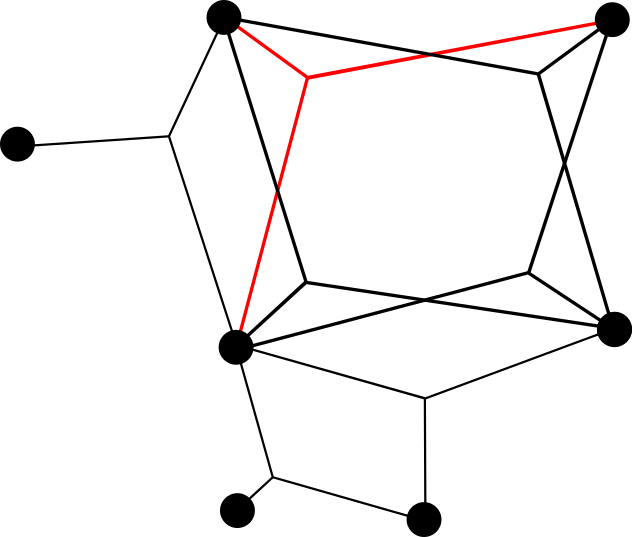
(a) Generalized Graph

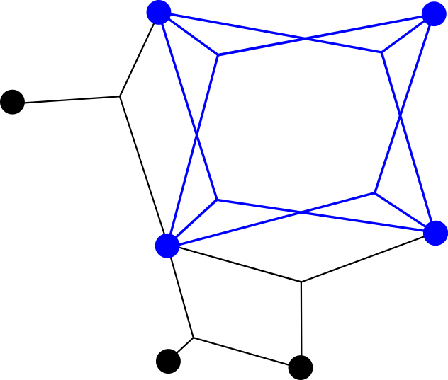
(b) Maximum Clique

Figure 1: An example of a generalized consistency graph with edges made of $3$-tuples. 1(a) highlights that each edge denotes consistency of $3$ measurements. 1(b) highlights the maximum clique of the generalized graph in blue.

IV-C Solving Group-$k$ Consistency Maximization

As with PCM, we can solve the G$k$CM problem by finding the maximum clique of a consistency graph. However, because we want to find the largest subset that is group-$k$ internally consistent we need to operate over generalized graphs. In graph theory, a k-uniform hypergraph (or generalized graph), $G$, is defined as a set of vertices $V$ and a set of $k$-tuples of those vertices $\mathcal{E}$ [21]. Each $k$-tuple is referred to as an edge and a clique within this context is a subgraph of $G$ where every possible edge is an edge in $\mathcal{E}$. We now introduce the concept of a generalized consistency graph:

Definition 2:

A generalized consistency graph is a generalized graph $G={V,\mathcal{E}}$ with $k$-tuple edges, where each vertex $v\in V$ represents a measurement and each edge $e\in\mathcal{E}$ denotes consistency of the vertices it connects.

Solving Eq. 3 is equivalent to finding the maximum clique of a generalized consistency graph and consists of the following two steps:

1. Building the generalized consistency graph

2. Finding the maximum clique

The next two sections explain these processes in more detail.

V Building the Generalized Consistency Graph

The graph is built by creating a vertex for each measurement and performing the relevant consistency checks to determine what edges should be added. If the graph is created all at once, their are $\binom{m}{k}$ checks to perform. If the graph is being built incrementally by checking the consistency of a new added measurement with those already in the graph then the number of checks is $\binom{m-1}{k-1}$. This means that as $k$ increases the number of checks that need to be performed increases factorially with $k$. Thus it is important that the consistency function in Eq. 2 be computationally efficient. Note that all the checks are independent allowing for the computation to be parallelized on a CPU or GPU to decrease the time to perform the necessary checks.

Algorithm 1 Exact Algorithm for Finding the Maximum Clique of a k-Uniform Hypergraph.
Input: Graph $G=(V,\mathcal{E})$, Output: Maximum Clique $S_{max}$

1:function MaxClique($G=(V,\mathcal{E})$)

2:    $S_{max}\leftarrow\emptyset$

3:    for $i=1$ to $n$ do

4:         if $d(v_{i})+1\geq|S_{max}|$ then

5:             for each $e\in E(v_{i})$ do

6:                 $S\leftarrow e\cup v_{i};$ $U\leftarrow\emptyset$

7:                 $R\leftarrow$ CombinationsOfSize($S,k-1$)

8:                 for each $v_{j}\in N(v_{i})$ do

9:                     if $j>i$ then

10:                         if $d(v_{j})+1\geq|S_{max}|$ then

11:                             if $R\subset E(v_{j})$ then

12:                                 $U\leftarrow U\cup\{v_{j}\}$                                                                                             

13:                 Clique($G,R,S,U$)                           

14:

15:

16:

17:

18:

1:function Clique($G=(V,\mathcal{E})$, $R$, $S$, $U$)

2:    if $U=\emptyset$ then

3:         if $|S|>|S_{max}|$ then

4:             $S_{max}\leftarrow S$              

5:    while $|U|>0$ do

6:         if $|S|+|U|\leq|S_{max}|$ then

7:             return          

8:         Select any vertex $u$ from $U$

9:         $U\leftarrow U\setminus\{u\};~{}S_{rec}\leftarrow S\cup\{u\}$

10:         $N^{\prime}(u):=\{w|w\in N(u)$ and $d(w)\geq|S_{max}|\}$

11:         $U_{rec}\leftarrow\emptyset;~{}R_{rec}\leftarrow R$

12:         for each $p\in$ CombinationsOfSize($S,k-2$) do

13:             $R_{rec}\leftarrow R_{rec}\cup\{p\cup\{u\}\}$          

14:         for each $q\in U\cap N^{\prime}(u)$ do

15:             if $R_{rec}\subset E(q)$ then

16:                 $U_{rec}\leftarrow U_{rec}\cup\{q\}$                       

17:         Clique($G,R_{rec},S_{rec},U_{rec}$)     

VI Finding the Maximum Clique of a Generalized Graph

Once the graph has been built, we can find the largest consistent set by finding the maximum clique of the graph. The PCM algorithm used the exact and heuristic methods presented by [11] but these algorithms were not designed for generalized graphs and used only a single thread. Here we generalize their algorithms to $k$-uniform hypergraphs and provide a parallelized implementation of their algorithms.

Figure 2: Examples of the degree, neighborhood, and edge set definitions for generalized graphs.

Algorithm 2 Heuristic Algorithm for Finding the Maximum Clique of a k-Uniform Hypergraph.
Input: Graph $G=(V,\mathcal{E})$, Output: Potential Maximum Clique $S_{max}$

1:function MaxCliqueHeu($G=(V,\mathcal{E})$)

2:    $S_{max}\leftarrow\emptyset$

3:    for $i=1$ to $n$ do

4:         if $d(v_{i})+1\geq|S_{max}|$ then

5:             Select $e\in E(v_{i})$ with max connect. in $E(v_{i})$

6:             $S\leftarrow e\cup v_{i};$ $U\leftarrow\emptyset$

7:             $R\leftarrow$ CombinationsOfSize($S,k-1$)

8:             for each $v_{j}\in N(v_{i})$ do

9:                 if $d(v_{j})+1\geq|S_{max}|$ then

10:                     if $R\subset E(v_{j})$ then

11:                         $U\leftarrow U\cup\{v_{j}\}$                                                    

12:             if $|S|+|U|>|S_{max}|$ then

13:                 CliqueHeu($G,R,S,U$)                           

14:

1:function CliqueHeu($G=(V,\mathcal{E})$, $R$, $S$, $U$)

2:    if $U=\emptyset$ then

3:         if $|S|>|S_{max}|$ then

4:             $S_{max}\leftarrow S$              

5:    Select a vertex $u\in U$ with max connect. in $E(v_{i})$

6:    $U\leftarrow U\setminus\{u\};~{}S_{rec}\leftarrow S\cup\{u\}$

7:    $N^{\prime}(u):=\{w|w\in N(u)$ and $d(w)\geq|S_{max}|\}$

8:    $U_{rec}\leftarrow\emptyset;~{}R_{rec}\leftarrow R$

9:    for each $p\in$ CombinationsOfSize($S,k-2$) do

10:         $R_{rec}\leftarrow R_{rec}\cup\{p\cup\{u\}\}$     

11:    for each $q\in U\cap N^{\prime}(u)$ do

12:         if $R_{rec}\subset E(q)$ then

13:             $U_{rec}\leftarrow U_{rec}\cup\{q\}$              

14:    CliqueHeu($G,R_{rec},S_{rec},U_{rec}$)

We start by defining relevant notation. We denote the $n$ vertices of the graph $G=(V,\mathcal{E})$ as $\{v_{1},\cdots,v_{n}\}$. Each vertex has a neighborhood $N(v_{i})$, that is the set of vertices connected to that vertex by at least one edge. The degree of $v_{i}$, $d(v_{i})$, is the number of vertices in its neighborhood. We also define an edge set, $E(v_{i})$, for each vertex consisting of a set of $(k-1)$-tuples of vertices. The edge set is derived from the set of $k$-tuples in $\mathcal{E}$ containing the given vertex by removing the given vertex from each edge. Figure 2 shows an example of these values for a given graph.

VI-A Algorithm Overview

The generalized exact and heuristic algorithms presented in Algorithm 1 and Algorithm 2 respectively are similar in structure to the algorithms in [11] but require additional checks to guarantee a valid clique is found since the algorithms now operate over generalized graphs.

The exact algorithm, Algorithm 1, begins with a vertex $v$ and finds cliques of size $k$ that contain $v$ (MaxClique line 5). A set of vertices, $U$, that would increase the clique size by one is found (MaxClique line 11) from the set of edges $R$ that a valid candidate vertex must have (MaxClique line 7). The Clique function then recursively iterates through potential cliques and updates $R$ and $U$ (Clique lines 13, 16). The clique is tracked with $S$ and a check is performed to see if $S>S_{max}$ where $S_{max}$ is replaced with $S$ if the check passes. The process is repeated for each vertex in the graph (MaxClique line 3). The exact algorithm evaluates all possible cliques and as such, the time complexity of the exact algorithm is exponential in worse case.

The heuristic algorithm, Algorithm 2, has a similar structure to the exact algorithm but uses a greedy search to find a potential maximum clique more quickly. For each node with a degree greater than the size of the current maximum clique (MaxCliqueHeu line 4) the algorithm selects a clique of size $k$ who has the greatest number of connections in $E(v_{i})$ (MaxCliqueHeu line 5). This is done by summing the number of connections each node in $N(v_{i})$ has in $E(v_{i})$ and selecting the edge $e\in E(v_{i})$ with the sum total of connections. It the selected clique can potentially be made larger than $S_{max}$ then a greedy search selects nodes based on the largest number of connections in $E(v_{i})$ (CliqueHeu line 5). The heruistic algorithm presented in Algorithm 2 has the same complexity of $O(n\Delta^{2})$ presented in [11] despite the modifications made to operate on generalized graphs.

Both algorithms are gauranteed to find a valid clique and can be easily parallelized by using multiple threads to simultaneously evaluate each iteration of the for loop on line 3 of MaxClique and MaxCliqueHeu. This significantly decreases the run-time of the algorithm. Our released C++ implementation allows the user to specify the number of threads to be used.

VI-B Evaluation of $\operatorname{MaxClique}$ and $\operatorname{MaxCliqueHeu}$

We carried out two experiments to evaluate the effectiveness of Algorithm 1 and Algorithm 2.

VI-B1 Timing Comparison

In the first experiment, we randomly generated 3-uniform hypergraphs with various node counts ranging from 25 vertices to 300 vertices. Each graph contained all the edges necessary to contain a maximum clique of cardinality 10 and additional randomly selected edges to meet a specified graph density. While the run-time of the algorithm is dependent on the density of the graph, for this experiment, we chose to hold the density of the graph constant at 0.1 such that approximately 10 percent of all potential edges were contained in the graph. We generated 100 sample graphs for each number of nodes. We then used both the exact and heuristic algorithm to estimate the maximum clique of each graph and measured the average run-time for each. Figure 3 shows the results of this experiment using various numbers of threads ranging from one to eight. The exact algorithm was only used for graphs with a total number of nodes of 100 or less because of the exponential nature of the algorithm.

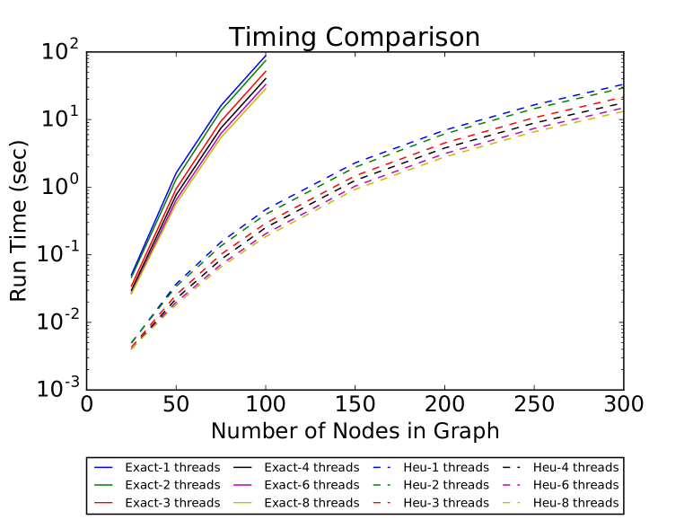
Figure 3: Average run-time for both the exact and heuristic generalized maximum clique algorithms proposed in this paper. This includes both the time to evaluate the necessary data-structures such as neighborhoods/edge sets and the time to estimate the maximum clique. Using eight threads, the heuristic algorithm was able to find the maximum clique of a graph with 250 nodes in a few seconds.

VI-B2 Heuristic Evaluation

In the second experiment, we again randomly generated 3-uniform hypergraphs, however, in this case we varied the density of the graph and the size of the inserted clique, while holding the total number of nodes at 100. For each graph we used the MaxCliqueHeu algorithm to estimate the maximum clique and then evaluated whether or not the algorithm was successful in finding a clique of the same size as the clique we inserted. We again generated 100 sample graphs for each combination of inserted-clique size and graph density. Figure 4 plots the summarized results. If the algorithm happened to return a maximum-clique larger, then the inserted clique than the associated sample was dropped.

This experiment shows that the size of the maximum clique and the success rate of the proposed heuristic algorithm are correlated. In addition, it shows that with the exception of the case when the inserted clique was very small (cardinality 5), the density of the graph and the success rate are inversely correlated. As such, the heuristic seems to perform best when the size of the maximum clique is large and/or when the connectivity of the graph is relatively sparse.

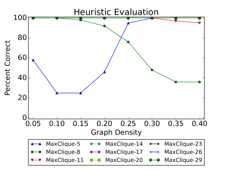
Figure 4: Evaluation of the heuristic algorithm proposed in Algorithm 2. Individual lines denote the cardinality of the maximum clique inserted into the graph. The horizontal axis denotes the density of edges in the graph and the vertical axis denotes the percentage of test cases where the algorithm returned a clique of the correct cardinality. The heuristic algorithm returned cliques of the correct size 100 percent of the time for the graphs with max clique size of 14, 17, 20, 23, 26, and 29.

VII Range-based SLAM

For the remainder of this paper we will consider G$k$CM in the context of a range-based SLAM scenario and will use the following $k=4$ consistency check,

$$\centering\begin{gathered}C(\boldsymbol{\mathrm{r}}_{ai},\boldsymbol{\mathrm{r}}_{bi},\boldsymbol{\mathrm{r}}_{ci},\boldsymbol{\mathrm{r}}_{di})=\left\lVert{h(\boldsymbol{\mathrm{X}}_{abcd},\boldsymbol{\mathrm{R}}_{abc}^{i})-\boldsymbol{\mathrm{r}}_{di}}\right\rVert_{\Sigma}\leq\gamma\end{gathered}\@add@centering$$ (4)

where $\boldsymbol{\mathrm{r}}_{di}$ is a range measurement from pose $d$ to beacon $i$, $\boldsymbol{\mathrm{X}}_{abcd}$ is a tuple of poses $a$, $b$, $c$, and $d$, and $\boldsymbol{\mathrm{R}}_{abc}^{i}$ is a tuple of range measurements from poses $a$, $b$, and $c$ to beacon $i$. The value $\gamma$ is a threshold value and the function $h(\boldsymbol{\mathrm{X}}_{abcd},\boldsymbol{\mathrm{R}}_{abc}^{i})$ is a measurement model defined as

$$\centering h(\boldsymbol{\mathrm{X}}_{abcd},\boldsymbol{\mathrm{R}}_{abc}^{i})=\left\lVert{\boldsymbol{\mathrm{l}}(\boldsymbol{\mathrm{X}}_{abc},\boldsymbol{\mathrm{R}}_{abc}^{i})-\boldsymbol{\mathrm{p}}_{d}}\right\rVert_{2}\@add@centering$$ (5)

where $\boldsymbol{\mathrm{X}}_{abc}$ is a tuple of poses $a$, $b$, and $c$, and $\boldsymbol{\mathrm{p}}_{i}$ is the position of pose $i$. The function $\boldsymbol{\mathrm{l}}(\boldsymbol{\mathrm{X}}_{abc},\boldsymbol{\mathrm{R}}_{abc}^{i})$ is a trilateration function that depends on the poses and the range measurements received at poses $a$, $b$, and $c$ and returns an estimate of the beacon’s location. The covariance, $\Sigma$, is a function of the covariances on the measurements $\boldsymbol{\mathrm{r}}$ and the poses $\boldsymbol{\mathrm{x}}$. The joint covariance, $\Sigma_{j}$, of the poses and beacon location are calculated by forming the measurement Jacobian of a factor graph and using methods described in [22]. Once the joint covariance has been obtained the covariance is calculated as $\Sigma=H\Sigma_{T}H^{T}$ where $H=\frac{\partial h}{\partial\boldsymbol{\mathrm{x}},\boldsymbol{\mathrm{l}},\boldsymbol{\mathrm{r}}_{d}}$ and $\Sigma_{T}=\mathit{blockdiag}(\Sigma_{j},\Sigma_{r_{d}})$.

The metric checks that the range to the intersection point of three range measurements matches the range of the fourth measurement. The check is done four times for a given set of four measurements where each permutation of three measurements is used to localize the beacon. Given the combinatorial nature of the number of checks to be performed, the trilateration algorithm needs to be fast and accurate. The algorithm described in [23] fits these criteria and presents a closed form algorithm that performs comparably to an iterative nonlinear optimization approach but without the need for an initial guess or an iterative solver.

VII-A Degenerate Configurations

Since our consistency check defined in Eq. 4 uses a trilateration algorithm we need to discuss the scenarios where trilateration fails to provide a unique solution. The first case is where the poses are collinear as shown in Fig. 5 and the second is when two of the three poses occupy the same position. The trilateration algorithm in [23] can return two estimates for the beacon’s location and the consistency check can pass if either estimate is deemed consistent.

If such a solution is not available, then a test to detect a degeneracy can be designed. If the test indicates the poses are in a degenerate configuration, the scenario can be handled by storing one or more of the measurements in a buffer whose consistency with the maximum clique can be tested after the clique has been found. If a degeneration is still present then the consistency of the measurement must be tested another way or the measurement be labeled inconsistent. In practice, we found that degenerate configurations did not present an issue because the odometry noise caused pose estimates used in the consistency check to not be degenerate even when the true configuration of poses was degenerate.

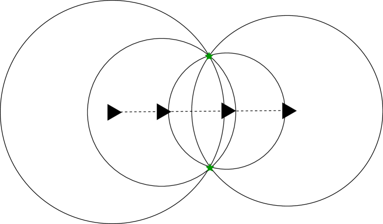
Figure 5: Degenerate pose configuration where range measurements do not result in a unique landmark location.

VIII Results

In this section we evaluate the performance of G$k$CM on several synthetic datasets where a robot is exploring and taking range measurements to static beacons. We compare the results of G$k$CM to the results of PCM where the consistency check for PCM is the check used in [8]. Due to runtime constraints all results are presented using the heuristic algorithm presented in Algorithm 2.

VIII-A Simulated 2D World

First we simulate a two-dimensional world where a robot is navigating in the plane. We simulate three different trajectories, (Manhattan world, circular, and a straight line) along with range measurements to static beacons placed randomly in the world. Gaussian noise was added to all range measurements and a portion of the measurements were corrupted to simulate outlier measurements. Half of the corrupted measurements were generated in clusters of size 5 and the other half as single random measurements using a Gaussian distribution with a random mean and a known variance. We assume that the variances of the range measurements are known and that these variances are used when performing the consistency check. The simulation was run multiple times varying values such as the trajectory and beacon locations, and statistics were recorded to compare G$k$CM with PCM.

VIII-A1 Monte Carlo Experiment

This first example was done to show how well G$k$CM performs in situations with large percentages of outliers. In this experiment a trajectory of 100 poses was simulated with measurements being taken at each pose and 80 of the measurements were corrupted to be outliers. G$k$CM was used to identify consistent measurements which were used used to solve the range-based SLAM problem in Eq. 1 using GTSAM [1]. The experiment averaged statistics over 81 runs and results are shown in Table I. G$k$CM outperforms PCM in every metric except the number of inliers found. Since to goal is to reject outliers, excluding a certain number of inliers is acceptable as long as outliers are also excluded. We primarily use the true positive rate (TPR), false positive rate (FPR) and $\chi^{2}$ value to evaluate how well how G$k$CM and PCM perform. Ideal values for these statistics are respectively 1, 0 and $\chi^{2}<3.84$ indicating the estimates fit the measurements with 95% confidence. Additionally, we show the median $\chi^{2}$ value. The large difference between the mean and the median, as well as the large standard deviation indicate that G$k$CM is performs better than the mean indicates. Looking at the $\chi^{2}$ values from all runs shows that the mean is greater than 75% of all the values showing that the times when G$k$CM failed skewed the mean. Figure 6 shows a sample map output by GTSAM when using the set of measurements selected by G$k$CM.

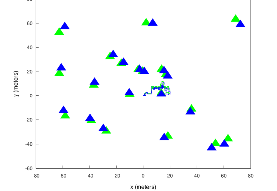
Figure 6: A larger experiment where 80 percent of the measurements are outliers. The green line and triangles are the true trajectory and beacon locations respectively while blue are the estimated trajectory and locations.

TABLE I: Statistics for G$k$CM and PCM in Monte Carlo experiment. Best results are in BOLD

	Trans. RMSE (m)		Rot. RMSE (rad)		Beacon Error (m)		Residual		Inliers		$\chi^{2}$
	Avg	Std	Avg	Std	Avg	Std	Avg	Std	TPR	FPR	Avg	Std	Median
G$k$CM	1.9774	1.8509	0.2805	0.077	12.118	28.114	442.82	948.3	0.85	0.007	2.28	4.94	0.56
PCM	7.8664	8.3322	0.5767	0.2405	26.883	43.502	18460	23355	0.92	0.026	89.68	111.26	52.69

Additionally, we wished to know at what ratio of outliers to inliers did the performance of G$k$CM begin to drop off. To measure this we simulated robot odometry for 100 poses and corrupted the measurements taken to a beacon with enough outliers to achieve a certain percentage of outliers. We ran the set of measurements through G$k$CM and observed if the selected set of consistent measurements matched the set of inlier measurements. Using the same robot odometry, this was done with several different outlier percentages. The process was repeated for multiple trajectories and the true/false positive rates for each outlier percentage were recorded. Results can be seen in Fig. 7.

The figure shows that the true and false positive rates for G$k$CM are fairly constant until about 85 percent of the measurements are outliers while the true positive rate decreases with the number of outliers for PCM and the false positive rate increases. These results are expected because as more outliers are present, it is more likely that either an outlier clique will form or that an outlier measurement will intersect with the inlier set with a pairwise basis than a group-4 basis. Thus showing the need for group consistency.

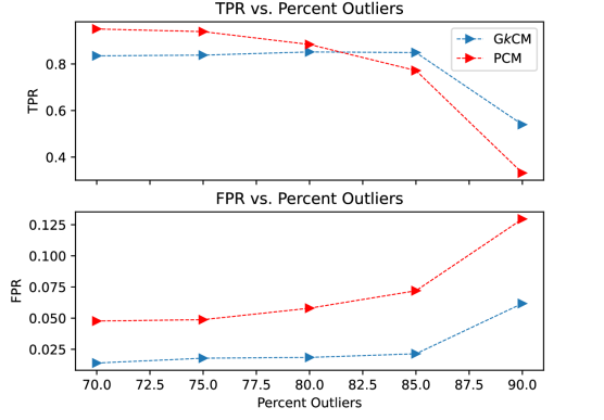
Figure 7: Results showing the normalized TPR ($\mathit{TP}/(\mathit{TP}+\mathit{FN}))$ and FPR $\mathit{FP}/(\mathit{FP}+\mathit{TN})$ by varying the number of outliers for a fixed trajectory.

VIII-B Data Association

In this experiment we remove the assumption that the correspondence between a range measurement and its beacon is known. To accomplish this, we modified both the exact and heuristic algorithms in order to track the $n$ largest cliques where $n$ is the number of beacons in the environment assuming the number of beacons is known. Since each clique corresponds to consistent measurements that belong to a unique beacon, we enforce the constraint that a measurement cannot appear in more than one clique.

This experiment was run on a short trajectory of 30 poses where five measurements were received at each pose (one to each beacon). As such there are 150 measurements being considered by the G$k$CM algorithm. Results were averaged over 81 different trials. Visual results can be seen in Fig. 8 while statistics are in Table II. G$k$CM correctly identifies the 5 cliques corresponding to the different beacons and out performs PCM in all the metrics.

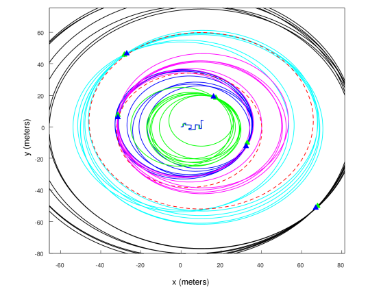
Figure 8: Results of G$k$CM for performing data association and outlier rejection. Each clique found is shown in a different color. Measurements labeled as outliers included in the maximum clique are red dashed lines.

TABLE II: Statistics for G$k$CM and PCM in Data Association experiment. Best results are in BOLD

	Translational RMSE (m)		Rotational RMSE (rad)		Beacon Error (m)		Residual		Inliers		Chi2
	Avg	Std	Avg	Std	Avg	Std	Avg	Std	TPR	FPR	Avg	Std	Median
G$k$CM	0.6259	0.5646	0.2469	0.0629	34.14	52.06	72.12	88.67	0.84	0.008	1.05	1.26	0.306
PCM	3.153	3.611	0.4521	0.2218	40.28	51.03	1010	1037	0.95	0.017	13.87	14.16	29.28

VIII-C Tuning Experiment

PCM has the nice property that changing the threshold value, $\gamma$, did not significantly impact the results of the algorithm. Due to enforced group consistency as opposed to pairwise we designed an experiment to test if G$k$CM has a similar property. We accomplished this by fixing a robot trajectory of 50 poses and the associated measurements and running G$k$CM multiple times with a different value for $\gamma$ each time. The measurements contained 40 outliers that were generated as described previously. We averaged the $\chi^{2}$ value and the true and false positive rates over multiple runs. Figure 9 shows how the above values vary with the consistency threshold for both G$k$CM and PCM.

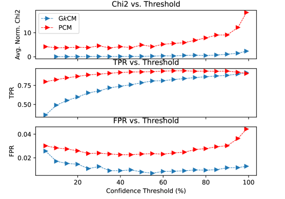
Figure 9: Results showing the normalized chi2 value, TPR and FPR by varying the consistency threshold value, $\gamma$, for a fixed trajectory.

As can be seen, G$k$CM performs better than PCM in both the normalized $\chi^{2}$ and false positive rate, which is more important in our application than the true positive rate. The results indicate that the performance of G$k$CM varies more with the threshold $\gamma$ than results in [7], especially at very low and high confidence thresholds. As such, we recommend that confidence values be used from the $50-90\%$ confidence range where performance was less variable with the confidence threshold.

VIII-D Incremental Update

In this last experiment we evaluate the incremental heuristic described in [19] since their experiments only evaluated the heuristic for a $k$-uniform hypergraph where $k=2$. For this experiment we generate a trajectory of 100 poses and measurements and at each step we evaluate how long both an incremental and batch update take. Updates include performing the consistency checks and finding the maximum clique. We record the runtime for the graph size and average statistics over multiple runs. We plot the runtime against the size of the graph in Fig. 10.

As can be seen the incremental update with the heuristic in [19] provides similar benefits for G$k$CM as it does for PCM. On average, for a graph of 100 nodes with 80 outliers, it takes a batch solution over 40 seconds to solve for the maximum clique while it takes only 3 seconds for the incremental update. These findings validate the results in [19] and also allow for G$k$CM to be run closer to real time.

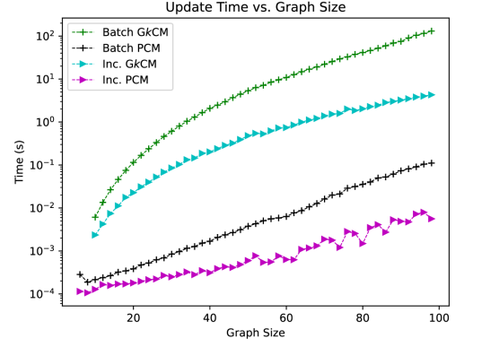
Figure 10: Timing data for both batch and incremental updates for G$k$CM and PCM. This includes the time to perform the relevant consistency checks and the new maximum clique. Note the log-scale on the vertical axis.

IX Conclusion

In this paper we introduced a novel concept called group-$k$ consistency maximization or G$k$CM. By modifying existing maximum clique algorithms to work over generalized graphs we can select groups of consistent measurements in high outlier regimes where pairwise consistency is inadequate.

References

- [1] M. Kaess, H. Johannsson, R. Roberts, V. Ila, J. J. Leonard, and F. Dellaert, “iSAM2: Incremental smoothing and mapping using the Bayes tree,” The International Journal of Robotics Research, vol. 31, no. 2, pp. 216–235, 2012.
- [2] G. Grisetti, R. Kümmerle, H. Strasdat, and K. Konolige, “g2o: A general framework for (hyper) graph optimization,” in Proceedings of the IEEE International Conference on Robotics and Automation (ICRA), 2011, pp. 9–13.
- [3] S. Agarwal, K. Mierle, et al., “Ceres solver,” 2012.
- [4] N. Sünderhauf and P. Protzel, “Towards a robust back-end for pose graph SLAM,” in 2012 IEEE international conference on robotics and automation. IEEE, 2012, pp. 1254–1261.
- [5] P. Agarwal, G. D. Tipaldi, L. Spinello, C. Stachniss, and W. Burgard, “Robust map optimization using dynamic covariance scaling,” in 2013 IEEE International Conference on Robotics and Automation. IEEE, 2013, pp. 62–69.
- [6] Y. Latif, C. Cadena, and J. Neira, “Robust loop closing over time for pose graph SLAM,” The International Journal of Robotics Research, vol. 32, no. 14, pp. 1611–1626, 2013.
- [7] J. G. Mangelson, D. Dominic, R. M. Eustice, and R. Vasudevan, “Pairwise consistent measurement set maximization for robust multi-robot map merging,” in 2018 IEEE International Conference on Robotics and Automation (ICRA). IEEE, 2018, pp. 2916–2923.
- [8] E. Olson, M. R. Walter, S. J. Teller, and J. J. Leonard, “Single-cluster spectral graph partitioning for robotics applications.” in Robotics: Science and Systems, 2005, pp. 265–272.
- [9] J. Shi, H. Yang, and L. Carlone, “ROBIN: a graph-theoretic approach to reject outliers in robust estimation using invariants,” in 2021 IEEE International Conference on Robotics and Automation (ICRA). IEEE, 2021, pp. 13 820–13 827.
- [10] P. C. Lusk, K. Fathian, and J. P. How, “Clipper: A graph-theoretic framework for robust data association,” in 2021 IEEE International Conference on Robotics and Automation (ICRA). IEEE, 2021, pp. 13 828–13 834.
- [11] B. Pattabiraman, M. M. A. Patwary, A. H. Gebremedhin, W.-k. Liao, and A. Choudhary, “Fast algorithms for the maximum clique problem on massive graphs with applications to overlapping community detection,” Internet Mathematics, vol. 11, no. 4-5, pp. 421–448, 2015.
- [12] P. Ozog, N. Carlevaris-Bianco, A. Kim, and R. M. Eustice, “Long-term mapping techniques for ship hull inspection and surveillance using an autonomous underwater vehicle,” Journal of Field Robotics, vol. 33, no. 3, pp. 265–289, 2016.
- [13] H. Yang, P. Antonante, V. Tzoumas, and L. Carlone, “Graduated non-convexity for robust spatial perception: From non-minimal solvers to global outlier rejection,” IEEE Robotics and Automation Letters, vol. 5, no. 2, pp. 1127–1134, 2020.
- [14] E. Olson and P. Agarwal, “Inference on networks of mixtures for robust robot mapping,” The International Journal of Robotics Research, vol. 32, no. 7, pp. 826–840, 2013.
- [15] A. M. Andrew, “Multiple view geometry in computer vision,” Kybernetes, 2001.
- [16] L. Sun, “Iron: Invariant-based highly robust point cloud registration,” arXiv preprint arXiv:2103.04357, 2021.
- [17] L. Carlone, A. Censi, and F. Dellaert, “Selecting good measurements via 1 relaxation: A convex approach for robust estimation over graphs,” in 2014 IEEE/RSJ International Conference on Intelligent Robots and Systems. IEEE, 2014, pp. 2667–2674.
- [18] T. Bailey, E. M. Nebot, J. Rosenblatt, and H. F. Durrant-Whyte, “Data association for mobile robot navigation: A graph theoretic approach,” in Proceedings 2000 ICRA. Millennium Conference. IEEE International Conference on Robotics and Automation. Symposia Proceedings (Cat. No. 00CH37065), vol. 3. IEEE, 2000, pp. 2512–2517.
- [19] Y. Chang, Y. Tian, J. P. How, and L. Carlone, “Kimera-multi: a system for distributed multi-robot metric-semantic simultaneous localization and mapping,” in 2021 IEEE International Conference on Robotics and Automation (ICRA). IEEE, 2021, pp. 11 210–11 218.
- [20] H. Do, S. Hong, and J. Kim, “Robust loop closure method for multi-robot map fusion by integration of consistency and data similarity,” IEEE Robotics and Automation Letters, vol. 5, no. 4, pp. 5701–5708, 2020.
- [21] B. Bollobás, “On generalized graphs,” Acta Mathematica Hungarica, vol. 16, no. 3-4, pp. 447–452, 1965.
- [22] M. Kaess and F. Dellaert, “Covariance recovery from a square root information matrix for data association,” Robotics and autonomous systems, vol. 57, no. 12, pp. 1198–1210, 2009.
- [23] Y. Zhou, “A closed-form algorithm for the least-squares trilateration problem,” Robotica, vol. 29, no. 3, pp. 375–389, 2011.