Learning Interpretable Temporal Properties from Positive Examples Only

Abstract

We consider the problem of explaining the temporal behavior of black-box systems using human-interpretable models. Following recent research trends, we rely on the fundamental yet interpretable models of deterministic finite automata (DFAs) and linear temporal logic (LTL_f) formulas. In contrast to most existing works for learning DFAs and LTL_f formulas, we consider learning from only positive examples. Our motivation is that negative examples are generally difficult to observe, in particular, from black-box systems. To learn meaningful models from positive examples only, we design algorithms that rely on conciseness and language minimality of models as regularizers. Our learning algorithms are based on two approaches: a symbolic and a counterexample-guided one. The symbolic approach exploits an efficient encoding of language minimality as a constraint satisfaction problem, whereas the counterexample-guided one relies on generating suitable negative examples to guide the learning. Both approaches provide us with effective algorithms with minimality guarantees on the learned models. To assess the effectiveness of our algorithms, we evaluate them on a few practical case studies.

1 Introduction

The recent surge of complex black-box systems in Artificial Intelligence has increased the demand for designing simple explanations of systems for human understanding. Moreover, in several areas such as robotics, healthcare, and transportation (Royal-Society, 2019; Gunning et al., 2019; Molnar, 2022), inferring human-interpretable models has become the primary focus to promote human trust in systems.

To enhance the interpretability of systems, we aim to explain their temporal behavior. For this purpose, models that are typically employed include, among others, finite state machines and temporal logics (Weiss et al., 2018; Roy et al., 2020). Our focus is on two fundamental models: deterministic finite automata (DFAs) (Rabin and Scott, 1959); and formulas in the de facto standard temporal logic: linear temporal logic (LTL) (Pnueli, 1977). These models not only possess a host of desirable theoretical properties, but also feature easy-to-grasp syntax and intuitive semantics. The latter properties make them particularly suitable as interpretable models with many applications, e.g., as task knowledge for robotic agents (Kasenberg and Scheutz, 2017; Memarian et al., 2020), as a formal specification for verification (Lemieux et al., 2015), as behavior classifier for unseen data (Shvo et al., 2021), and several others (Camacho and McIlraith, 2019).

The area of learning DFAs and LTL formulas is well-studied with a plethora of existing works (see related work). Most of them tackle the typical binary classification problem (Gold, 1978) of learning concise DFAs or LTL formulas from a finite set of examples partitioned into a positive and a negative set. However, negative examples are hard to obtain in my scenarios. In safety-critical areas, often observing negative examples from systems (e.g., from medical devices and self-driving cars) can be unrealistic (e.g., by injuring patients or hitting pedestrians). Further, often one only has access to a black-box implementation of the system and thus, can extract only its possible (i.e., positive) executions.

In spite of being relevant, the problem of learning concise DFAs and LTL formulas from positive examples, i.e., the corresponding one class classification (OCC) problem, has garnered little attention. The primary reason, we believe, is that, like most OCC problems, this problem is an ill-posed one. Specifically, a concise model that classifies all the positive examples correctly is the trivial model that classifies all examples as positive. This corresponds to a single state DFA or, in LTL, the formula $\mathit{true}$. These models, unfortunately, convey no insights about the underlying system.

To ensure a well-defined problem, Avellaneda and Petrenko (2018), who study the OCC problem for DFAs, propose the use of the (accepted) language of a model (i.e., the set of allowed executions) as a regularizer. Searching for a model that has minimal language, however, results in one that classifies only the given examples as positive. To avoid this overfitting, they additionally impose an upper bound on the size of the model. Thus, the OCC problem that they state is the following: given a set of positive examples $P$ and a size bound $n$, learn a DFA that (a) classifies $P$ correctly, (b) has size at most $n$, and (c) is language minimal. For language comparison, the order chosen is set inclusion.

To solve this OCC problem, Avellaneda and Petrenko (2018) then propose a counterexample-guided algorithm. This algorithm relies on generating suitable negative examples (i.e., counterexamples) iteratively to guide the learning process. Since only the negative examples dictate the algorithm, in many iterations of their algorithm, the learned DFAs do not have a language smaller (in terms of inclusion) than the previous hypothesis DFAs. This results in searching through several unnecessary DFAs.

To alleviate this drawback, our first contribution is a symbolic algorithm for solving the OCC problem for DFA. Our algorithm converts the search for a language minimal DFA symbolically to a series of satisfiability problems in Boolean propositional logic, eliminating the need for counterexamples. The key novelty is an efficient encoding of the language inclusion check of DFAs in a propositional formula, which is polynomial in the size of the DFAs. We then exploit an off-the-shelf SAT solver to check satisfiability of the generated propositional formulas and, thereafter, construct a suitable DFA. We expand on this algorithm in Section 3.

We then present two novel algorithms for solving the OCC problem for formulas in LTL_f (LTL over finite traces). While our algorithms extend smoothly to traditional LTL (over infinite traces), our focus here is on LTL_f due to its numerous applications in AI (Giacomo and Vardi, 2013). Also, LTL_f being a strict subclass of DFAs, the learning algorithms for DFAs cannot be applied directly to learn LTL_f formulas.

Our first algorithm for LTL_f is a semi-symbolic algorithm, which combines ideas from both the symbolic and the counterexample-guided approaches. Roughly, this algorithm exploits negative examples to overcome the theoretical difficulties of symbolically encoding language inclusion for LTL_f. (LTL_f inclusion check is known to be inherently harder than that for DFAs (Sistla and Clarke, 1985)). Our second algorithm is simply a counterexample-guided algorithm that relies solely on the generation of negative examples for learning. Section 4 details both algorithms.

To further study the presented algorithms, we empirically evaluate them in several case studies. We demonstrate that our symbolic algorithm solves the OCC problem for DFA in fewer (approximately one-tenth) iterations and runtime comparable to the counterexample-guided algorithm, skipping thousands of counterexample generations. Further, we demonstrate that our semi-symbolic algorithm solves the OCC problem for LTL_f (in average) thrice as fast as the counterexample-guided algorithm. All our experimental results can be found in Section 5.

1.0.1 Related Work.

The OCC problem described in this paper belongs to the body of works categorized as passive learning (Gold, 1978). As alluded to in the introduction, in this topic, the most popular problem is the binary classification problem for learning DFAs and LTL formulas. Notable works include the works by Biermann and Feldman (1972); Grinchtein et al. (2006); Heule and Verwer (2010) for DFAs and Neider and Gavran (2018a); Camacho and McIlraith (2019); Raha et al. (2022) for LTL/LTL_f.

The OCC problem of learning formal models from positive examples was first studied by Gold (1967). This work showed that the exact identification (in the limit) of certain models (that include DFAs and LTL_f formulas) from positive examples is not possible. Thereby, works have mostly focussed on models that are learnable easily from positive examples, such as pattern languages (Angluin, 1980), stochastic finite state machines (Carrasco and Oncina, 1999), and hidden Markov Models (Stolcke and Omohundro, 1992). None of these works considered learning DFAs or LTL formulas, mainly due to the lack of a meaningful regularizer.

Recently, Avellaneda and Petrenko (2018) proposed the use of language minimality as a regularizer and, thereafter, developed an effective algorithm for learning DFAs. While their algorithm cannot overcome the theoretical difficulties shown by Gold (1967), they still produce a DFA that is a concise description of the positive examples. We significantly improve upon their algorithm by relying on a novel encoding of language minimality using propositional logic.

For temporal logics, there are a few works that consider the OCC problem. Notably, Ehlers et al. (2020) proposed a learning algorithm for a fragment of LTL which permits a representation known as universally very-weak automata (UVWs). However, since their algorithm relies on UVWs, which has strictly less expressive power than LTL, it cannot be extended to full LTL. Further, there are works on learning LTL (Chou et al., 2022) and STL (Jha et al., 2019) formulas from trajectories of high-dimensional systems. These works based their learning on the assumption that the underlying system optimizes some cost functions. Our method, in contrast, is based on the natural notion of language minimality to find tight descriptions, without any assumptions on the system. There are some other works that consider the OCC problem for logics similar to temporal logic (Xu et al., 2019b, a; Stern and Juba, 2017).

A problem similar to our OCC problem is studied in the context of inverse reinforcement learning (IRL) to learn temporal rewards for RL agents from (positive) demonstrations. For instance, Kasenberg and Scheutz (2017) learn concise LTL formulas that can distinguish between the provided demonstrations from random executions of the system. To generate the random executions, they relied on a Markov Decision Process (MDP) implementation of the underlying system. Our regularizers, in contrast, assume the underlying system to be a black-box and need no access to its internal mechanisms. Vazquez-Chanlatte et al. (2018) also learn LTL-like formulas from demonstrations. Their search required a pre-computation of the lattice of formulas induced by the subset order, which can be a bottleneck for scaling to full LTL. Recently, Hasanbeig et al. (2021) devised an algorithm to infer automaton for describing high-level objectives of RL agents. Unlike ours, their algorithm relied on user-defined hyper-parameters to regulate the degree of generalization of the inferred automaton.

2 Preliminaries

In this section, we set up the notation for the rest of the paper.

Let $\mathbb{N}=\{1,2,\ldots\}$ be the set of natural numbers and $[n]=\{1,2,\ldots,n\}$ be the set of natural numbers up to $n$.

2.0.1 Words and Languages.

To formally represent system executions, we rely on the notion of words, defined over a finite and nonempty alphabet $\Sigma$. The elements of $\Sigma$, which denote relevant system states, are referred to as symbols.

A word over $\Sigma$ is a finite sequence $w=a_{1}\ldots a_{n}$ with $a_{i}\in\Sigma$, $i\in[n]$. The empty word $\varepsilon$ is the empty sequence. The length $|w|$ of $w$ is the number of symbols in it (note that $|\varepsilon|=0$). Moreover, $\Sigma^{\ast}$ denotes the set of all words over $\Sigma$. Further, we use $w[i]=a_{i}$ to denote the $i$-th symbol of $w$ and $w[i{:}]=a_{i}\cdots a_{n}$ to denote the suffix of $w$ starting from position $i$.

A language $L$ is any set of words from $\Sigma^{\ast}$. We allow the standard set operations on languages such as $L_{1}\subseteq L_{2}$, $L_{1}\subset L_{2}$ and $L_{1}\setminus L_{2}$.

2.0.2 Propositional logic.

All our algorithms rely on propositional logic and thus, we introduce it briefly. Let $\mathit{Var}$ be a set of propositional variables, which take Boolean values $\{0,1\}$ ($0$ represents $\mathit{false}$, $1$ represents $\mathit{true}$). Formulas in propositional logic—which we denote by capital Greek letters—are defined recursively as

$$\Phi\coloneqq x\in\mathit{Var}\mid\neg\Phi\mid\Phi\lor\Phi.$$

As syntax sugar, we allow the following standard formulas: $\mathit{true}$, $\mathit{false}$, $\Phi\land\Psi$, $\Phi\rightarrow\Psi$, and $\Phi\leftrightarrow\Psi$.

An assignment $v\colon\mathit{Var}\mapsto\{0,1\}$ maps propositional variables to Boolean values. Based on an assignment $v$, we define the semantics of propositional logic using a valuation function $V(v,\Phi)$, which is inductively defined as follows:

$$V(v,x) =v(x)$$

$$V(v,\neg\Psi) =1-V(v,\Psi)$$

$$V(v,\Psi\lor\Phi) =\mathit{max}\{V(v,\Psi),V(v,\Phi)\}$$

We say that $v$ satisfies $\Phi$ if $V(v,\Phi)=1$, and call $v$ a model of $\Phi$. A formula $\Phi$ is satisfiable if there exists a model $v$ of $\Phi$.

Arguably, the most well-known problem in propositional logic—the satisfiability (SAT) problem—is the problem of determining whether a propositional formula is satisfiable or not. With the rapid development of SAT solvers (Li and Manyà, 2021), checking satisfiability of formulas with even millions of variables is feasible. Most solvers can also return a model when a formula is satisfiable.

3 Learning DFA from Positive Examples

In this section, we present our symbolic algorithm for learning DFAs from positive examples. We begin by formally introducing DFAs.

A deterministic finite automaton (DFA) is a tuple $\mathcal{A}=(Q,\Sigma,\delta,q_{I},F)$ where $Q$ is a finite set of states, $\Sigma$ is the alphabet, $q_{I}\in Q$ is the initial state, $F\subseteq Q$ is the set of final states, and $\delta\colon Q\times\Sigma\to Q$ is the transition function. We define the size $|\mathcal{A}|$ of a DFA as its number of states $|Q|$.

Given a word $w=a_{1}\ldots a_{n}\in\Sigma^{\ast}$, the run of $\mathcal{A}$ on $w$, denoted by $\mathcal{A}\colon q_{1}\xrightarrow{w}q_{n+1}$, is a sequence of states and symbols $q_{1}a_{1}q_{2}a_{2}\cdots a_{n}q_{n+1}$, such that $q_{1}=q_{I}$ and for each $i\in[n]$, $q_{i+1}=\delta({q_{i},a_{i}})$. Moreover, we say $w$ is accepted by $\mathcal{A}$ if the last state in the run $q_{n+1}\in F$. Finally, we define the language of $\mathcal{A}$ as $L({\mathcal{A}})=\{w\in\Sigma^{\ast}~{}|~{}w\text{ is accepted by }\mathcal{A}\}$.

To introduce the OCC problem for DFAs, we first describe the learning setting. The OCC problem relies on a set of positive examples, which we represent using a finite set of words $P\subset\Sigma^{\ast}$. Additionally, the problem requires a bound $n$ to restrict the size of the learned DFA. The role of this size bound is two-fold: (1) it ensures that the learned DFA does not overfit $P$; and (2) using a suitable bound, one can enforce the learned DFAs to be concise and, thus, interpretable.

Finally, we define a DFA $\mathcal{A}$ to be an $n\textrm{-description}$ of $P$ if $P\subseteq L({\mathcal{A}})$ and $|\mathcal{A}|\leq n$. When $P$ is clear from the context, we simply say $\mathcal{A}$ is an $n\textrm{-description}$.

We can now state the OCC problem for DFAs:

Problem 1 (OCC problem for DFAs)

Given a set of positive words $P$ and a size bound $n$, learn a DFA $\mathcal{A}$ such that: (1) $\mathcal{A}$is an $n\textrm{-description}$; and (2) for every DFA $\mathcal{A}^{\prime}$ that is an $n\textrm{-description}$, $L(\mathcal{A}^{\prime})\not\subset L(\mathcal{A})$.

Intuitively, the above problem asks to search for a DFA that is an $n\textrm{-description}$ and has a minimal language. Note that several such DFAs can exist since the language inclusion is a partial order on the languages of DFA. We, here, are interested in learning only one such DFA, leaving the problem of learning all such DFAs as interesting future work.

3.1 The Symbolic Algorithm

We now present our algorithm for solving Problem 1. Its underlying idea is to reduce the search for an appropriate DFA to a series of satisfiability checks of propositional formulas. Each satisfiable propositional formula enables us to construct a guess, or a so-called hypothesis DFA $\mathcal{A}$. In each step, using the hypothesis $\mathcal{A}$, we construct a propositional formula $\Phi^{\mathcal{A}}$ to search for the next hypothesis $\mathcal{A}^{\prime}$ with a language smaller (in the inclusion order) than the current one. The properties of the propositional formula $\Phi^{\mathcal{A}}$ we construct are: (1) $\Phi^{\mathcal{A}}$is satisfiable if and only if there exists a DFA $\mathcal{A}^{\prime}$ that is an $n\textrm{-description}$ and $L({\mathcal{A}^{\prime}})\subset L({\mathcal{A}})$; and (2) based on a model $v$ of $\Phi^{\mathcal{A}}$, one can construct a such a DFA $\mathcal{A}^{\prime}$.

Based on the main ingredient $\Phi^{\mathcal{A}}$, we design our learning algorithm as sketched in Algorithm 1. Our algorithm initializes the hypothesis DFA $\mathcal{A}$ to be $\mathcal{A}_{\Sigma^{\ast}}$, which is the one-state DFA that accepts all words in $\Sigma^{\ast}$. Observe that $\mathcal{A}_{\Sigma^{\ast}}$ is trivially an $n\textrm{-description}$, since $P\subset\Sigma^{\ast}$ and $|\mathcal{A}_{\Sigma^{\ast}}|=1$. The algorithm then iteratively exploits $\Phi^{\mathcal{A}}$ to construct the next hypothesis DFAs, until $\Phi^{\mathcal{A}}$ becomes unsatisfiable. Once this happens, we terminate and return the current hypothesis $\mathcal{A}$ as the solution. The correctness of this algorithm follows from the following theorem:

Theorem 3.1

Given positive words $P$ and a size bound $n$, Algorithm 1 always learns a DFA $\mathcal{A}$ that is an $n\textrm{-description}$ and for every DFA $\mathcal{A}^{\prime}$ that is an $n\textrm{-description}$, $L({\mathcal{A}^{\prime}})\not\subset L({\mathcal{A}})$.

Algorithm 1 Symbolic Algorithm for Learning DFA

Input: Positive words $P$, bound $n$

1:  $\mathcal{A}\leftarrow\mathcal{A}_{\Sigma^{\ast}}$, $\Phi^{\mathcal{A}}\coloneqq\Phi_{\mathtt{DFA}}\wedge\Phi_{P}$

2:  while $\Phi^{\mathcal{A}}$ is satisfiable (with model $v$) do

3:     $\mathcal{A}\leftarrow$ DFA constructed from $v$

4:     $\Phi^{\mathcal{A}}\coloneqq\Phi_{\mathtt{DFA}}\wedge\Phi_{P}\wedge\Phi_{\subseteq\mathcal{A}}\wedge\Phi_{\not\supseteq\mathcal{A}}$

5:  end while

6:  return  $\mathcal{A}$

We now expand on the construction of $\Phi^{\mathcal{A}}$. To achieve the aforementioned properties, we define $\Phi^{\mathcal{A}}$ as follows:

$$\Phi^{\mathcal{A}}\coloneqq\Phi_{\mathtt{DFA}}\wedge\Phi_{P}\wedge\Phi_{\subseteq\mathcal{A}}\wedge\Phi_{\not\supseteq\mathcal{A}}$$ (1)

The first conjunct $\Phi_{\mathtt{DFA}}$ ensures that the propositional variables we will use encode a valid DFA $\mathcal{A}^{\prime}$. The second conjunct $\Phi_{P}$ ensures that $\mathcal{A}^{\prime}$ accepts all positive words. The third conjunct $\Phi_{\subseteq\mathcal{A}}$ ensures that $L({\mathcal{A}^{\prime}})$ is a subset of $L({\mathcal{A}})$. The final conjunct $\Phi_{\not\supseteq\mathcal{A}}$ ensures that $L({\mathcal{A}^{\prime}})$ is not a superset of $L({\mathcal{A}})$. Together, conjuncts $\Phi_{\subseteq\mathcal{A}}$ and $\Phi_{\not\supseteq\mathcal{A}}$ ensure that $L({\mathcal{A}^{\prime}})$ is a proper subset of $L({\mathcal{A}})$. In what follows, we detail the construction of each conjunct.

To encode the hypothesis DFA $\mathcal{A}^{\prime}=(Q^{\prime},\Sigma,\delta^{\prime},{q^{\prime}_{I}},F^{\prime})$ symbolically, following Heule and Verwer (2010), we rely on the propositional variables: (1) $d_{p,a,q}$where $p,q\in[n]$ and $a\in\Sigma$; and (2) $f_{q}$where $q\in[n]$. The variables $d_{p,a,q}$ and $f_{q}$ encode the transition function $\delta^{\prime}$ and the final states $F^{\prime}$, respectively, of $\mathcal{A}^{\prime}$. Mathematically speaking, if $d_{p,a,q}$ is set to true, then $\delta^{\prime}(p,a)=q$ and if $f_{q}$ is set to true, then $q\in F^{\prime}$. Note that we identify the states $Q^{\prime}$ using the set $[n]$ and the initial state ${q^{\prime}_{I}}$ using the numeral 1.

Now, to ensure $\mathcal{A}^{\prime}$ has a deterministic transition function $\delta^{\prime}$, $\Phi_{\mathtt{DFA}}$ asserts the following constraint:

$$\bigwedge_{p\in[n]}\bigwedge_{a\in\Sigma}\Big{[}\bigvee_{q\in[n]}d_{p,a,q}\wedge\bigwedge_{q\neq q^{\prime}\in[n]}\big{[}\neg d_{p,a,q}\vee\neg d_{p,a,q^{\prime}}\big{]}\Big{]}$$ (2)

Based on a model $v$ of the variables $d_{p,a,q}$ and $f_{q}$, we can simply construct $\mathcal{A}^{\prime}$. We set $\delta^{\prime}(p,a)$ to be the unique state $q$ for which $v(d_{p,a,q})=1$ and $q\in F^{\prime}$ if $v(f_{q})=1$.

Next, to construct conjunct $\Phi_{P}$, we introduce variables $x_{u,q}$ where $u\in\mathit{Pref}(P)$ and $q\in[n]$, which track the run of $\mathcal{A}^{\prime}$ on all words in $\mathit{Pref}(P)$, which is the set of prefixes of all words in $P$. Precisely, if $x_{u,q}$ is set to true, then there is a run of $\mathcal{A}^{\prime}$ on $u$ ending in state $q$, i.e., $\mathcal{A}^{\prime}\colon{q^{\prime}_{I}}\xrightarrow{u}q$.

Using the introduced variables, $\Phi_{P}$ ensures that the words in $P$ are accepted by imposing the following constraints:

$$x_{\varepsilon,1}\wedge\bigwedge_{q\in\{2,\ldots,n\}}\neg x_{\varepsilon,q}$$ (3)

$$\bigwedge_{ua\in\mathit{Pref}(P)}\bigwedge_{p,q\in[n]}[x_{u,p}\wedge d_{p,a,q}]\operatorname{\rightarrow}x_{ua,q}$$ (4)

$$\bigwedge_{w\in P}\bigwedge_{q\in[n]}x_{w,q}\operatorname{\rightarrow}f_{q}$$ (5)

The first constraint above ensures that the runs start in the initial state ${q^{\prime}_{I}}$ (which we denote using 1) while the second constraint ensures that they adhere to the transition function. The third constraint ensures that the run of $\mathcal{A}^{\prime}$ on every $w\in P$ ends in a final state and is, hence, accepted.

For the third conjunct $\Phi_{\subseteq\mathcal{A}}$, we must track the synchronized runs of the current hypothesis $\mathcal{A}$ and the next hypothesis $\mathcal{A}^{\prime}$ to compare their behavior on all words in $\Sigma^{\ast}$. To this end, we introduce auxiliary variables, $y^{\mathcal{A}}_{q,q^{\prime}}$ where $q,q^{\prime}\in[n]$. Precisely, $y^{\mathcal{A}}_{q,q^{\prime}}$ is set to true, if there exists a word $w\in\Sigma^{\ast}$ such that there are runs $\mathcal{A}\colon q_{I}\xrightarrow{w}q$ and $\mathcal{A}^{\prime}\colon{q^{\prime}_{I}}\xrightarrow{w}q^{\prime}$.

To ensure $L({\mathcal{A}^{\prime}})\subseteq L({\mathcal{A}})$, $\Phi_{\subseteq\mathcal{A}}$ imposes the following constraints:

$$y^{\mathcal{A}}_{1,1}$$ (6)

$$\bigwedge_{q=\delta({p,a})}\bigwedge_{p^{\prime},q^{\prime}\in[n]}\bigwedge_{a\in\Sigma}\Big{[}\big{[}y^{\mathcal{A}}_{p,p^{\prime}}\wedge d_{p^{\prime},a,q^{\prime}}\big{]}\rightarrow y^{\mathcal{A}}_{q,q^{\prime}}\Big{]}$$ (7)

$$\bigwedge_{p\not\in F}\bigwedge_{p^{\prime}\in[n]}\Big{[}y^{\mathcal{A}}_{p,p^{\prime}}\rightarrow\neg f_{p^{\prime}}\Big{]}$$ (8)

The first constraint ensures that the synchronized runs of $\mathcal{A}$ and $\mathcal{A}^{\prime}$ start in the respective initial states, while the second constraint ensures that they adhere to their respective transition functions. The third constraint ensures that if the synchronized run ends in a non-final state in $\mathcal{A}$, it must also end in a non-final state in $\mathcal{A}^{\prime}$, hence forcing $L(\mathcal{A}^{\prime})\subseteq L(\mathcal{A})$.

For constructing the final conjunct $\Phi_{\not\supset\mathcal{A}}$, the variables we exploit rely the following result:

Lemma 1

Let $\mathcal{A}$, $\mathcal{A}^{\prime}$ be DFAs such that $|\mathcal{A}|=|\mathcal{A}^{\prime}|=n$ and $L({\mathcal{A}^{\prime}})\subset L({\mathcal{A}})$, and let $K=n^{2}$. Then there exists a word $w\in\Sigma^{\ast}$ such that $|w|\leq K$ and $w\in L({\mathcal{A}})\setminus L({\mathcal{A}^{\prime}})$.

This result provides an upper bound to the length of a word that can distinguish between DFAs $\mathcal{A}$ and $\mathcal{A}^{\prime}$

Based on this result, we introduce variables $z_{i,q,q^{\prime}}$ where $i\in[n^{2}]$ and $q,q^{\prime}\in[n]$ to track the synchronized run of $\mathcal{A}$ and $\mathcal{A}^{\prime}$ on a word of length at most $K=n^{2}$. Precisely, if $z_{i,q,q^{\prime}}$ is set to true, then there exists a word $w$ of length $i$, with the runs $\mathcal{A}\colon q_{I}\xrightarrow{w}q$ and $\mathcal{A}^{\prime}:q_{I}^{\prime}\xrightarrow{w}q^{\prime}$.

Now, $\Phi_{\not\supseteq\mathcal{A}}$ imposes the following constraints:

$$z_{0,1,1}$$ (9)

$$\bigwedge_{i\in[n^{2}]}\Big{[}\bigvee_{q,q^{\prime}\in[n]}z_{i,q,q^{\prime}}\wedge\big{[}\bigwedge_{\begin{subarray}{c}p\neq q\in[n]\\ p^{\prime}\neq q^{\prime}\in[n]\end{subarray}}\neg z_{i,p,p^{\prime}}\vee\neg z_{i,q,q^{\prime}}\big{]}\Big{]}$$ (10)

$$\bigwedge_{\begin{subarray}{c}p,q\in[n]\\ p^{\prime},q^{\prime}\in[n]\end{subarray}}\Big{[}\big{[}z_{i,p,p^{\prime}}\wedge z_{i+1,q,q^{\prime}}\big{]}\operatorname{\rightarrow}\bigvee_{\begin{subarray}{c}a\in\Sigma\text{ where}\\ {q=\delta(p,a)}\end{subarray}}d_{p^{\prime},a,q^{\prime}}\Big{]}$$ (11)

$$\bigvee_{i\in[n^{2}]}\bigvee_{\begin{subarray}{c}q\in F\\ q^{\prime}\in[n]\end{subarray}}\Big{[}z_{i,q,q^{\prime}}\wedge\neg f_{q^{\prime}}\Big{]}$$ (12)

The first three constraints above ensure that words up to length $n^{2}$ have a valid synchronised run on the two DFAs $\mathcal{A}$ and $\mathcal{A}^{\prime}$. The final constraint ensures that there is a word of length $\leq n^{2}$ on which the synchronized run ends in a final state in $\mathcal{A}$ but not in $\mathcal{A}^{\prime}$, ensuring $L(\mathcal{A})\not\subseteq L(\mathcal{A}^{\prime})$.

We now prove the correctness of the propositional formula $\Phi^{\mathcal{A}}$ that we construct using the above constraints:

Theorem 3.2

Let $\Phi^{\mathcal{A}}$ be as defined above. Then, we have the following:

1. If $\Phi^{\mathcal{A}}$ is satisfiable, then there exists a DFA $\mathcal{A}^{\prime}$ that is an $n\textrm{-description}$ and $L({\mathcal{A}^{\prime}})\subset L({\mathcal{A}})$.

2. If there exists a DFA $\mathcal{A}^{\prime}$ that is an $n\textrm{-description}$ and $L({\mathcal{A}^{\prime}})\subset L({\mathcal{A}})$, then $\Phi^{\mathcal{A}}$ is satisfiable.

To prove the above theorem, we propose intermediate claims, all of which we prove first. For the proofs, we assume $\mathcal{A}=(Q,\Sigma,\delta,{q_{I}},F)$ to be the current hypothesis, $v$ to be a model of $\Phi^{\mathcal{A}}$, and $\mathcal{A}^{\prime}=(Q^{\prime},\Sigma,\delta^{\prime},{q^{\prime}_{I}},F^{\prime})$ to be the DFA constructed from the model $v$ of $\Phi^{\mathcal{A}}$.

Claim 1

For all $u\in\mathit{Pref}(P)$, $\mathcal{A}^{\prime}:{q^{\prime}_{I}}\xrightarrow{u}q$ implies $v(x_{u,q})=1$.

Proof

We prove the claim using induction on the length $|u|$ of the word $u$.

Base case:

Let $u=\varepsilon$. Based on the definition of runs, $\mathcal{A}^{\prime}:{q^{\prime}_{I}}\xrightarrow{\epsilon}q$ implies $q={q^{\prime}_{I}}$. Also, using Constraint 3, we have $v(x_{\varepsilon,q})=1$ if and only if $q={q^{\prime}_{I}}$ (note $q^{\prime}_{I}$ is indicated using numeral 1). Combining these two facts proves the claim for the base case.

Induction step:

As induction hypothesis, let $\mathcal{A}^{\prime}:{q_{I}}^{\prime}\xrightarrow{u}q$ implies $v(x_{u,q})=1$ for all words $u\in\mathit{Pref}(P)$ of length $\leq k$. Now, consider the run $\mathcal{A}^{\prime}:{q^{\prime}_{I}}\xrightarrow{u}q\xrightarrow{a}q^{\prime}$ for some $ua\in\mathit{Pref}(P)$. For this run, based on the induction hypothesis and the construction of $\mathcal{A}^{\prime}$, we have $v(x_{u,q})=1$ and $v(d_{p,a,q})=1$. Now, using Constraint 4, $v(x_{u,q})=1$ and $v(d_{p,a,q})=1$ implies $v(x_{ua,q})=1$, thus, proving the claim.

∎

Claim 2

For all $w\in\Sigma^{\ast}$, $\mathcal{A}:q_{I}\xrightarrow{w}q$ and $\mathcal{A}^{\prime}:{q^{\prime}_{I}}\xrightarrow{w}q^{\prime}$ imply $v(y^{\mathcal{A}}_{q,q^{\prime}})=1$.

Proof

We prove this using induction of the length $|w|$ of the word $w$.

Base case:

Let $w=\varepsilon$. Based on the definition of runs, $\mathcal{A}:{q_{I}}\xrightarrow{\varepsilon}q$, $\mathcal{A}^{\prime}:{q^{\prime}_{I}}\xrightarrow{\varepsilon}q^{\prime}$ implies $q={q_{I}}$ and $q={q^{\prime}_{I}}$. Also, using Constraint 6, $q=q_{I}$ and $q^{\prime}={q^{\prime}_{I}}$ imply $v(y^{\mathcal{A}}_{q,q^{\prime}})=1$ (note $q_{I}$ and $q^{\prime}_{I}$ are both indicated using numeral 1). Combining these two facts proves the claim for the base case.

Induction step:

As induction hypothesis, let $\mathcal{A}:{q_{I}}\xrightarrow{w}q$ and $\mathcal{A}^{\prime}:{q^{\prime}_{I}}\xrightarrow{w}q^{\prime}$ imply $v(y^{\mathcal{A}}_{q,q^{\prime}})=1$ for all words $w\in\Sigma^{\ast}$ of length $\leq k$. Now, consider the runs $\mathcal{A}:{q_{I}}\xrightarrow{w}p\xrightarrow{a}q$ and $\mathcal{A}^{\prime}:{q_{I}}^{\prime}\xrightarrow{w}p^{\prime}\xrightarrow{a}q^{\prime}$ for some word $wa\in\Sigma^{\ast}$ For these runs, based on the induction hypothesis and the construction of $\mathcal{A}^{\prime}$, we have $v(y^{\mathcal{A}}_{p,p^{\prime}})=1$ and $v(d_{p^{\prime},a,q^{\prime}})=1$. Now, using Constraint 7, we can say that $v(y^{\mathcal{A}}_{p,p^{\prime}})=1$ and $v(d_{p^{\prime},a,q^{\prime}})=1$ imply $v(y^{\mathcal{A}}_{q,q^{\prime}})=1$ (where $q=\delta(p,a)$), thus, proving the claim.

∎

Claim 3

$v(z_{i,q,q^{\prime}})=1$ implies there exists $w\in\Sigma^{i}$ with runs $\mathcal{A}:q_{I}\xrightarrow{w}q$ and $\mathcal{A}^{\prime}:{q^{\prime}_{I}}\xrightarrow{w}q^{\prime}$.

Proof

We prove this using induction on the parameter $i$.

Base case:

Let $i=0$. Based on the Constraints 9 and 10, $v(z_{0,q,q^{\prime}})=1$ implies $q={q_{I}}$ and $q={q_{I}}^{\prime}$. Now, there always exists a word of length $0$, $w=\varepsilon$, for which $\mathcal{A}:q_{I}\xrightarrow{\varepsilon}q$ and $\mathcal{A}^{\prime}:{q^{\prime}_{I}}\xrightarrow{\varepsilon}q^{\prime}$ proving the claim for the base case.

Induction step:

As induction hypothesis, let $v(z_{k,p,p^{\prime}})=1$ and thus, $w$ be a word of length $k$ such that $\mathcal{A}:q_{I}\xrightarrow{w}p$ and $\mathcal{A}^{\prime}:{q^{\prime}_{I}}\xrightarrow{w}p^{\prime}$. Now, assume $v(z_{k+1,q,q^{\prime}})=1$. Based on Constraint 11, for some $a\in\Sigma$ such that $q=\delta(p,a)$, $v(d_{p^{\prime},a,q^{\prime}})=1$. Thus, on the word $wa$, there are runs $\mathcal{A}:q_{I}\xrightarrow{w}p\xrightarrow{a}q$ and $\mathcal{A}^{\prime}:{q^{\prime}_{I}}\xrightarrow{w}p^{\prime}\xrightarrow{a}q^{\prime}$, proving the claim.

∎

We are now ready to prove Theorem 3.2, i.e., the correctness of $\Phi^{\mathcal{A}}$.

Proof (of Theorem 3.2)

For the forward direction, consider that $\Phi^{\mathcal{A}}$ is satisfiable with a model $v$ and $\mathcal{A}^{\prime}$ is the DFA constructed using the model $v$. First, using Claim 1, $\mathcal{A}^{\prime}\colon{q^{\prime}_{I}}\xrightarrow{w}q$ implies $v(x_{w,q})=1$ for all $w\in P$. Now, based on Constraint 5, $v(x_{w,q})=1$ implies $v(f_{q})=1$ for all $w\in P$. As a result, for each $w\in P$, its run $\mathcal{A}^{\prime}\colon{q^{\prime}_{I}}\xrightarrow{w}q$ must end in a final state $q\in F^{\prime}$ in $\mathcal{A}^{\prime}$. Thus, $\mathcal{A}^{\prime}$ accepts all positive words and hence, is an $n\textrm{-description}$. Second, using Claim 2, $\mathcal{A}:q_{I}\xrightarrow{w}q$ and $\mathcal{A}^{\prime}:{q^{\prime}_{I}}\xrightarrow{w}q^{\prime}$ imply $v(y^{\mathcal{A}}_{q,q^{\prime}})=1$ for all words $w\in\Sigma^{\ast}$. Thus, based on Constraint 8, if $q\not\in F$, then $q^{\prime}\not\in F$, implying $L({\mathcal{A}^{\prime}})\subseteq L({\mathcal{A}})$. Third, using Claim 3, $v(z_{i,q,q^{\prime}})=1$ implies that there exists $w\in\Sigma^{i}$ with runs $\mathcal{A}:q_{I}\xrightarrow{w}q$ and $\mathcal{A}^{\prime}:{q^{\prime}_{I}}\xrightarrow{w}q^{\prime}$. Now, based on Constraint 12, there exists some $i\leq n^{2}$, $q\in F$ and $q^{\prime}$ in $\mathcal{A}^{\prime}$ such that $v(z_{i,q,q^{\prime}})=1$ and $v(f_{q^{\prime}})=0$. Combining this fact with Claim 3, we deduce that there exists $w\in\Sigma^{\ast}$ with length $\leq n^{2}$ with run $\mathcal{A}:q_{I}\xrightarrow{w}q$ ending in final state $q\in F$ and run $\mathcal{A}^{\prime}:{q^{\prime}_{I}}\xrightarrow{w}q^{\prime}$ not ending in a final state $q^{\prime}\in F^{\prime}$. This shows that $L({\mathcal{A}})\neq L({\mathcal{A}^{\prime}})$. We thus conclude that $\mathcal{A}$ is an $n\textrm{-description}$ and $L({\mathcal{A}^{\prime}})\subset L({\mathcal{A}})$.

For the other direction, based on a suitable DFA $\mathcal{A}^{\prime}$, we construct an assignment $v$ for all the introduce propositional variables. First, we set $v(d_{p,a,q})=1$ if $\delta^{\prime}(p,a)=q$ and $v(f_{q})=1$ if $q\in F^{\prime}$. Since $\delta^{\prime}$ is a deterministic function, $v$ satisfies the Constraint 2. Similarly, we set $v(x_{u,q})=1$ if $\mathcal{A}^{\prime}\colon{q^{\prime}_{I}}\xrightarrow{u}q$ for some $u\in\mathit{Pref}(P)$. It is a simple exercise to check that $v$ satisfies Constraints 3 to 5. Next, we set $v(y^{\mathcal{A}}_{q,q^{\prime}})=1$ if there are runs $\mathcal{A}\colon q_{I}\xrightarrow{w}q$ and $\mathcal{A}^{\prime}\colon{q^{\prime}_{I}}\xrightarrow{w}q^{\prime}$ on some word $w\in\Sigma^{\ast}$. Algorithmically, we set $v(y^{\mathcal{A}}_{q,q^{\prime}})=1$ if states $q$ and $q^{\prime}$ are reached in the synchronized run of $\mathcal{A}$ and $\mathcal{A}^{\prime}$ on some word (which is typically computed using a breadth-first search on the product DFA). It is easy to see that such an assignment $v$ satisfies Constraints 6 to 8. Finally, we set assignment to $z_{i,q,q^{\prime}}$ exploiting a word $w$ which permits runs $\mathcal{A}\colon q_{I}\xrightarrow{w}q$ and $\mathcal{A}^{\prime}\colon{q^{\prime}_{I}}\xrightarrow{w}q^{\prime}$, where $q$ is in $F$ but $q^{\prime}$ not in $F^{\prime}$. In particular, we set $v(z_{i,q,q^{\prime}})=1$ for $i=|u|$ and $\mathcal{A}\colon q_{I}\xrightarrow{u}q$ and $\mathcal{A}^{\prime}\colon{q^{\prime}_{I}}\xrightarrow{u}q^{\prime}$ for all prefixes $u$ of $w$. Such an assignment encodes a synchronized run of the DFAs $\mathcal{A}$ and $\mathcal{A}^{\prime}$ on word $w$ that ends in a final state in $\mathcal{A}$, but not in $\mathcal{A}^{\prime}$. Thus, $v$ satisfies Constraints 9 to 12. ∎

Proof (of Theorem 3.1)

First, observe that Algorithm 1 always terminates. This is because, there is finitely many $n\textrm{-description}$ for a given $n$ (following its definition) and in each iteration, the algorithm finds a new one. Next, observe that the algorithm terminates when $\Phi^{\mathcal{A}}$ is unsatisfiable. Now, based on the properties of $\Phi^{\mathcal{A}}$ established in Theorem 3.2, if $\Phi^{\mathcal{A}}$ is unsatisfiable for some DFA $\mathcal{A}$, then there are no $n\textrm{-description}$ DFA $\mathcal{A}^{\prime}$ for which $L(\mathcal{A}^{\prime})\subset L(\mathcal{A})$, thus, proving the correctness of the algorithm. ∎

4 Learning LTL_f formulas from Positive Examples

We now switch our focus to algorithms for learning LTL_f formulas from positive examples. We begin with a formal introduction to LTL_f.

Linear temporal logic (over finite traces) (LTL_f) is a logic that reasons about the temporal behavior of systems using temporal modalities. While originally LTL_f is built over propositional variables $\mathcal{P}$, to unify the notation with DFAs, we define LTL_f over an alphabet $\Sigma$. It is, however, not a restriction since an LTL_f formula over $\mathcal{P}$ can always be translated to an LTL_f formula over $\Sigma=2^{\mathcal{P}}$. Formally, we define LTL_f formulas—denoted by Greek small letters—inductively as:

$$\varphi\coloneqq a\in\Sigma\mid\lnot\varphi\mid\varphi\lor\varphi\mid\operatorname{\mathbf{X}}\varphi\mid\varphi\operatorname{\mathbf{U}}\varphi$$

As syntactic sugar, along with additional constants and operators used in propositional logic, we allow the standard temporal operators $\operatorname{\mathbf{F}}$ (“finally”) and $\operatorname{\mathbf{G}}$ (“globally”). We define $\Lambda=\{\lnot,\lor,\land,\operatorname{\rightarrow},\operatorname{\mathbf{X}},\operatorname{\mathbf{U}},\operatorname{\mathbf{F}},\operatorname{\mathbf{G}}\}~{}\cup~{}\Sigma$ to be the set of all operators (which, for simplicity, also includes symbols). We define the size $|\varphi|$ of $\varphi$ as the number of its unique subformulas; e.g., size of $\varphi=(a\operatorname{\mathbf{U}}\operatorname{\mathbf{X}}b)\lor\operatorname{\mathbf{X}}b$ is five, since its five distinct subformulas are $a,b,\operatorname{\mathbf{X}}b,a\operatorname{\mathbf{U}}\operatorname{\mathbf{X}}b$, and $(a\operatorname{\mathbf{U}}\operatorname{\mathbf{X}}b)\lor\operatorname{\mathbf{X}}b$.

To interpret LTL_f formulas over (finite) words, we follow the semantics proposed by Giacomo and Vardi (2013). Given a word $w$, we define recursively when a LTL_f formula holds at position $i$, i.e., $w,i\models\varphi$, as follows:

$$w,i\models a\in\Sigma\text{ if and only if }a=w[i]$$

$$w,i\models\lnot\varphi\text{ if and only if }w,i\not\models\varphi$$

$$w,i\models\operatorname{\mathbf{X}}\varphi\text{ if and only if }i<|w|\text{ and }w,i+1\models\varphi$$

$$w,i\models\varphi\operatorname{\mathbf{U}}\psi\text{ if and only if }w,j\models\psi\text{ for some }$$

$$\hskip 28.45274pti\leq j\leq|w|\text{ and }w,i^{\prime}\models\varphi\text{ for all }i\leq i^{\prime}<j$$

We say $w$ satisfies $\varphi$ or, alternatively, $\varphi$ holds on $w$ if $w,0\models\varphi$, which, in short, is written as $w\models\varphi$.

The OCC problem for LTL_f formulas, similar to Problem 1, relies upon a set of positive words $P\subset\Sigma^{\ast}$ and a size upper bound $n$. Moreover, an LTL_f formula $\varphi$ is an $n\textrm{-description}$ of $P$ if, for all $w\in P$, $w\models\varphi$, and $|\varphi|\leq n$. Again, we omit $P$ from $n\textrm{-description}$ when clear. Also, in this section, an $n\textrm{-description}$ refers only to an LTL formula.

We state the OCC problem for LTL_f formulas as follows:

Problem 2 (OCC problem for LTL_f formulas)

Given a set of positive words $P$ and a size bound $n$, learn an LTL_f formula $\varphi$ such that: (1) $\varphi$is an $n\textrm{-description}$; and (2) for every LTL_f formula $\varphi^{\prime}$ that is an $n\textrm{-description}$, $\varphi^{\prime}\not\rightarrow\varphi$ or $\varphi\rightarrow\varphi^{\prime}$.

Intuitively, the above problem searches for an LTL_f formula $\varphi$ that is an $n\textrm{-description}$ and holds on a minimal set of words. Once again, like Problem 1, there can be several such LTL_f formulas, but we are interested in learning exactly one.

4.1 The Semi-Symbolic Algorithm

Our semi-symbolic, does not only depend on the current hypothesis, an LTL_f formula $\varphi$ here, as was the case in Algorithm 1. In addition, it relies on a set of negative examples $N$, accumulated during the algorithm. Thus, using both the current hypothesis $\varphi$ and the negative examples $N$, we construct a propositional formula $\Psi^{\varphi,N}$ to search for the next hypothesis $\varphi^{\prime}$. Concretely, $\Psi^{\varphi,N}$ has the properties that: (1) $\Psi^{\varphi,N}$is satisfiable if and only if there exists an LTL_f formula $\varphi^{\prime}$ that is an $n\textrm{-description}$, does not hold on any $w\in N$, and $\varphi\not\rightarrow\varphi^{\prime}$; and (2) based on a model $v$ of $\Psi^{\varphi,N}$, one can construct such an LTL_f formula $\varphi^{\prime}$.

Algorithm 2 Semi-symbolic Algorithm for learning LTL_f formula

Input: Positive words $P$, bound $n$

1:  $N\leftarrow\emptyset$

2:  $\varphi\leftarrow\mathit{true}$, $\Psi^{\varphi,N}\coloneqq\Psi_{\mathtt{LTL}}\wedge\Psi_{P}$

3:  while $\Psi^{\varphi,N}$ is satisfiable (with model $v$) do

4:     $\varphi^{\prime}\leftarrow$ LTL formula constructed from $v$

5:     if $\varphi^{\prime}\rightarrow\varphi$ then

6:        Update $\varphi$ to $\varphi^{\prime}$

7:     else

8:        Add $w$ to $N$, where $w\models\neg\varphi^{\prime}\wedge\varphi$

9:     end if

10:     $\Psi^{\varphi,N}\coloneqq\Psi_{\mathtt{LTL}}\wedge\Psi_{P}\wedge\Psi_{N}\wedge\Psi_{\not\leftarrow\varphi}$

11:  end while

12:  return  $\varphi$

The semi-symbolic algorithm whose pseudocode is presented in Algorithm 2 follows a paradigm similar to the one illustrated in Algorithm 1. However, unlike the previous algorithm, the current guess $\varphi^{\prime}$, obtained from a model of $\Psi^{\varphi,N}$, may not always satisfy the relation $\varphi^{\prime}\rightarrow\varphi$. In such a case, we generate a word (i.e., a negative example) that satisfies $\varphi$, but not $\varphi^{\prime}$ to eliminate $\varphi^{\prime}$ from the search space. For the generation of words, we rely on constructing DFAs from the LTL_f formulas (Zhu et al., 2017) and then performing a breadth-first search over them. If, otherwise, $\varphi^{\prime}\rightarrow\varphi$, we then update our current hypothesis and continue until $\Psi^{\varphi,N}$ is unsatisfiable. Overall, this algorithm learns an appropriate LTL_f formula with the following guarantee:

Theorem 4.1

Given positive words $P$ and size bound $n$, Algorithm 2 learns an LTL_f formula $\varphi$ that is an $n\textrm{-description}$ and for every LTL_f formulas $\varphi^{\prime}$ that is an $n\textrm{-description}$, $\varphi^{\prime}\not\rightarrow\varphi$ or $\varphi\rightarrow\varphi^{\prime}$.

We now focus on the construction of $\Psi^{\varphi,N}$, which is significantly different from that of $\Phi^{\mathcal{A}}$. It is defined as follows:

$$\Psi^{\varphi,N}\coloneqq\Psi_{\mathtt{LTL}}\wedge\Psi_{P}\wedge\Psi_{N}\wedge\Psi_{\not\leftarrow\varphi}.$$ (13)

The first conjunct $\Psi_{\mathtt{LTL}}$ ensures that propositional variables we exploit encode a valid LTL_f formula $\varphi^{\prime}$. The second conjunct $\Psi_{P}$ ensures that $\varphi^{\prime}$ holds on all positive words, while the third, $\Psi_{N}$, ensures that it does not hold on the negative words. The final conjunct $\Phi_{\not\leftarrow\varphi}$ ensures that $\varphi\not\rightarrow\varphi^{\prime}$.

(a)

(b)

Figure 1: Syntax DAG and identifiers for $(a\operatorname{\mathbf{U}}\operatorname{\mathbf{X}}b)\vee\operatorname{\mathbf{X}}b$

Following Neider and Gavran (2018a), all of our conjuncts rely on a canonical syntactic representation of LTL_f formulas as syntax DAGs. A syntax DAG is a directed acyclic graph (DAG) that is obtained from the syntax tree of an LTL_f formula by merging its common subformulas. An example of a syntax DAG is illustrated in Figure LABEL:fig:syntax-dag. Further, to uniquely identify each node of a syntax DAG, we assign them unique identifiers from $[n]$ such that every parent node has an identifier larger than its children (see Figure LABEL:fig:identifier).

To construct the hypothesis $\varphi^{\prime}$, we encode its syntax DAG, using the following propositional variables: (1) $x_{i,\lambda}$for $i\in[n]$ and $\lambda\in\Lambda$; and (2) $l_{i,j}$and $r_{i,j}$ for $i\in[n]$ and $j\in[i{-}1]$. The variable $x_{i,\lambda}$ tracks the operator label of the Node $i$ of the syntax DAG of $\varphi^{\prime}$, while variables $l_{i,j}$ and $r_{i,j}$ encode the left and right child of Node $i$, respectively. Mathematically, $x_{i,\lambda}$ is set to true if and only if Node $i$ is labeled with operator $\lambda$. Moreover, $l_{i,j}$ (resp. $r_{i,j}$) is set to true if and only if Node $i$’s left (resp. right) child is Node $j$.

To ensure variables $x_{i,\lambda}$, $l_{i,j}$ and $r_{i,j}$ have the desired meaning, $\Psi_{\mathtt{LTL}}$ imposes certain structural constraints, which we list below.

$$\bigwedge_{i\in[n]}\Big{[}\bigvee_{\lambda\in\Lambda}x_{i,\lambda}\wedge\bigwedge_{\lambda\neq\lambda^{\prime}\in\Lambda}\big{[}\neg x_{i,\lambda}\vee\neg x_{i,\lambda^{\prime}}\big{]}\Big{]}$$ (14)

$$\bigwedge_{i\in\{2,\cdots,n\}}\Big{[}\bigvee_{j\in[i-1]}l_{i,j}\wedge\bigwedge_{j\neq j^{\prime}\in[i-1]}\big{[}\neg r_{i,j}\vee\neg l_{i,j^{\prime}}\big{]}\Big{]}$$ (15)

$$\bigwedge_{i\in\{2,\cdots,n\}}\Big{[}\bigvee_{j\in[i-1]}r_{i,j}\wedge\bigwedge_{j\neq j^{\prime}\in[i-1]}\big{[}\neg r_{i,j}\vee\neg r_{i,j^{\prime}}\big{]}\Big{]}$$ (16)

$$\bigvee_{a\in\Sigma}x_{1,a}$$ (17)

Constraint 14 ensures that each node of the syntax DAG of $\varphi^{\prime}$ is uniquely labeled by an operator. Constraints 15 and 16 encode that each node of the syntax DAG of $\varphi^{\prime}$ has a unique left and right child, respectively. Finally, Constraint 17 encodes that the node with identifier 1 must always be a symbol.

We now describe the construction of $\Psi_{P}$ and $\Psi_{N}$. Both use variables $y^{i}_{w,t}$ where $i\in[n]$, $w\in P\cup N$, and $t\in[|w|]$. The variable $y^{i}_{w,t}$ tracks whether $\varphi^{\prime}_{i}$ holds on the suffix $w[t{:}]$, where $\varphi^{\prime}_{i}$ is the subformula of $\varphi^{\prime}$ rooted at Node $i$. Formally, $y^{i}_{w,t}$ is set to true if and only if $w[t{:}]\models\varphi^{\prime}_{i}$.

To ensure the desired meaning of variables $y^{i}_{w,t}$, $\Psi_{P}$ and $\Psi_{N}$ impose semantic constraints, again to ones proposed by Neider and Gavran (2018a).

$$\bigwedge\limits_{i\in[n]}\bigwedge\limits_{a\in\Sigma}x_{i,a}\rightarrow\Big{[}\bigwedge\limits_{t\in[|w|]}\begin{cases}y^{i}_{w,t}\text{ if }a=w[t]\\ \neg y^{i}_{w,t}\text{ if }a\neq w[t]\end{cases}\Big{]}$$ (18)

$$\bigwedge\limits_{\begin{subarray}{c}i\in[n]\\ j,j^{\prime}\in[i-1]\end{subarray}}x_{i,\vee}\wedge l_{i,j}\wedge r_{i,j^{\prime}}\rightarrow\Big{[}\bigwedge\limits_{\begin{subarray}{c}\tau\in[|w|]\end{subarray}}\Big{[}y^{i}_{w,t}\leftrightarrow y^{j}_{w,t}\vee y^{j^{\prime}}_{w,t}\Big{]}\Big{]}$$ (19)

$$\bigwedge\limits_{\begin{subarray}{c}i\in[n]\\ j\in[i-1]\end{subarray}}x_{i,\operatorname{\mathbf{X}}}\land l_{i,j}\rightarrow\big{[}\bigwedge_{t\in[|w|-1]}y^{i}_{w,t}\leftrightarrow y^{j}_{w,t+1}\big{]}\wedge\neg y^{j}_{w,|w|}$$ (20)

$$\bigwedge\limits_{\begin{subarray}{c}i\in[n]\\ j,j^{\prime}\in[i]\end{subarray}}x_{i,\operatorname{\mathbf{U}}}\wedge l_{i,j}\wedge r_{i,j^{\prime}}\rightarrow\Big{[}\bigwedge\limits_{\begin{subarray}{c}t\in[|w|]\end{subarray}}\Big{[}y^{i}_{w,t}\leftrightarrow\bigvee\limits_{t\leq t^{\prime}\in[|w|]}\Big{[}y^{j^{\prime}}_{w,t^{\prime}}\wedge\bigwedge\limits_{t\leq\tau<t^{\prime}}y^{j}_{w,\tau}\Big{]}\Big{]}$$ (21)

Intuitively, the above constraints encode the meaning of the different LTL operators using propositional logic.

To ensure that $\varphi^{\prime}$ holds on positive words, we have $\Psi_{P}\coloneqq\bigwedge_{w\in P}y^{n}_{w,0}$ and to ensure $\varphi^{\prime}$ does not hold on negative words, we have $\Psi_{N}\coloneqq\bigwedge_{w\in N}\neg y^{n}_{w,0}$.

Next, to construct $\Psi_{\not\leftarrow\varphi}$, we symbolically encode a word $u$ that distinguishes formulas $\varphi$ and $\varphi^{\prime}$. We bound the length of the symbolic word by a time horizon $K=2^{2^{n+1}}$. The choice of $K$ is derived from Lemma 1 and the fact that the size of the equivalent DFA for an LTL_f formulas can be at most doubly exponential (Giacomo and Vardi, 2015).

Our encoding of a symbolic word $u$ relies on variables $p_{t,a}$ where $t\in[K]$ and $a\in\Sigma\cup\{\varepsilon\}$. If $p_{t,a}$ is set to true, then $u[t]=a$. To ensure that the variables $p_{t,a}$ encode their desired meaning, we generate a formula $\Psi_{\mathtt{word}}$ that consists of the following constraint:

$$\bigwedge_{t\in[K]}\Big{[}\bigvee_{a\in\Sigma\cup\{\varepsilon\}}p_{t,a}\wedge\bigwedge_{a\neq a^{\prime}\in\Sigma\cup\{\varepsilon\}}\big{[}\neg p_{t,a}\vee\neg p_{t,a^{\prime}}\big{]}\Big{]}$$ (22)

The above constraint ensures that, in the word $u$, each position $t\leq K$ has a unique symbol from $\Sigma\cup\{\varepsilon\}$.

Further, to track whether $\varphi$ and $\varphi^{\prime}$ hold on $u$, we have variables $z^{\varphi,i}_{u,t}$ and $z^{\varphi^{\prime},i}_{u,t}$ where $i\in[n]$, $t\in[K]$. These variables are similar to $y^{i}_{w,t}$, in the sense that $z^{\varphi,i}_{u,t}$ (resp. $z^{\varphi^{\prime},i}_{u,t}$) is set to true, if $\varphi$ (resp. $\varphi^{\prime}$) holds at position $t$. To ensure desired meaning of these variables, we impose semantic constraints $\Psi_{\mathtt{sem}}$, similar to the semantic constraints imposed on $y^{i}_{w,t}$. We list the constraints on the variables $z^{\varphi^{\prime},i}_{u,t}$.

$$\bigwedge\limits_{i\in[n]}\bigwedge\limits_{a\in\Sigma}x_{i,a}\rightarrow\Big{[}\bigwedge\limits_{t\in[K]}z^{\varphi^{\prime},i}_{u,t}\leftrightarrow p_{t,a}\Big{]}$$ (23)

$$\bigwedge\limits_{\begin{subarray}{c}i\in[n]\\ j,j^{\prime}\in[i-1]\end{subarray}}x_{i,\vee}\wedge l_{i,j}\wedge r_{i,j^{\prime}}\rightarrow\Big{[}\bigwedge\limits_{\begin{subarray}{c}t\in[K]\end{subarray}}\Big{[}z^{\varphi^{\prime},i}_{w,t}\leftrightarrow z^{\varphi^{\prime},j}_{u,t}\vee z^{\varphi^{\prime},j^{\prime}}_{u,t}\Big{]}\Big{]}$$ (24)

$$\bigwedge\limits_{\begin{subarray}{c}i\in[n]\\ j\in[i-1]\end{subarray}}x_{i,\operatorname{\mathbf{X}}}\land l_{i,j}\rightarrow\big{[}\bigwedge_{t\in[K-1]}z^{\varphi^{\prime},i}_{w,t}\leftrightarrow z^{\varphi^{\prime},j}_{u,t+1}\big{]}\wedge\neg z^{\varphi^{\prime},j}_{u,|w|}$$ (25)

$$\bigwedge\limits_{\begin{subarray}{c}i\in[n]\\ j,j^{\prime}\in[i]\end{subarray}}x_{i,\operatorname{\mathbf{U}}}\wedge l_{i,j}\wedge r_{i,j^{\prime}}\rightarrow\Big{[}\bigwedge\limits_{\begin{subarray}{c}t\in[K]\end{subarray}}\Big{[}z^{\varphi^{\prime},i}_{u,t}\leftrightarrow\bigvee\limits_{t\leq t^{\prime}\in[K]}\Big{[}z^{\varphi^{\prime},j^{\prime}}_{u,t^{\prime}}\wedge\bigwedge\limits_{t\leq\tau<t^{\prime}}z^{\varphi^{\prime},j}_{u,\tau}\Big{]}\Big{]}$$ (26)

Clearly, the above constraints are identical to the Constraints 18 to 21 imposed on variables $y^{i}_{w,t}$. The constraints on variables $z^{\varphi,i}_{w,t}$ are quite similar. The only difference is that for hypothesis $\varphi$, we know the syntax DAG exactly and thus, can exploit it instead of using an encoding of the syntax DAG.

Finally, we set $\Psi_{\not\leftarrow\varphi}\coloneqq\Psi_{\mathtt{word}}\wedge\Psi_{\mathtt{sem}}\wedge z^{\varphi,n}_{u,0}\wedge\neg z^{\varphi^{\prime},n}_{u,0}$. Intuitively, the above conjunction ensures that there exists a word on which $\varphi$ holds and $\varphi^{\prime}$ does not.

We now prove the correctness of the encoding $\Psi^{\varphi,N}$ described using the constraints above.

Theorem 4.2

Let $\Psi^{\varphi,N}$ be as defined above. Then, we have the following:

1. If $\Psi^{\varphi,N}$ is satisfiable, then there exists an LTL formula $\varphi^{\prime}$ that is an $n\textrm{-description}$, $\varphi^{\prime}$ does not hold on $w\in N$ and $\varphi\not\rightarrow\varphi^{\prime}$.

2. If there exists a LTL formula $\varphi^{\prime}$ that is an $n\textrm{-description}$, $\varphi^{\prime}$ does not hold on $w\in N$ and $\varphi\not\rightarrow\varphi^{\prime}$, then $\Psi^{\varphi,N}$ is satisfiable.

To prove this theorem, we rely on intermediate claims, which we state now. In the claims, $v$ is a model of $\Psi^{\varphi,N}$, $\varphi^{\prime}$ is the LTL formula constructed from $v$ and $\varphi$ is the current hypothesis LTL formula.

Claim 4

For all $w\in P\cup N$, $v(y^{i}_{w,t})=1$ if and only if $w[t{:}]\models\varphi^{\prime}[i]$.

The proof proceeds via structural induction over $\varphi^{\prime}[i]$. For the proof of this claim, we refer the readers to the correctness proof of the encoding used by (Neider and Gavran, 2018a) that can in found in their full paper (Neider and Gavran, 2018b).

Claim 5

$v(z^{\varphi^{\prime},i}_{w,t})=1$ (resp. $v(z^{\varphi,i}_{w,t})=1$) if and only for a word $w$, $w[t{:}]\models\varphi^{\prime}$ (resp. $w[t{:}]\models\varphi$).

The proof again proceeds via a structural induction on $\varphi^{\prime}$ (similar to the previous one).

We are now ready to prove Theorem 4.2, i.e., the correctness of $\Omega^{N,D}$.

Proof (of Theorem 4.2)

For the forward direction, consider that $\Psi^{\varphi,N}$ is satisfiable with a model $v$ and $\varphi^{\prime}$ is the LTL formula constructed using the model $v$. First, using Claim 4, we have that $v(y^{n}_{w,t})=1$ if and only if $w[t{:}]\models\varphi^{\prime}$. Now, based on the constraints $\Psi_{P}$ and $\Psi_{N}$, we observe that $v(y^{n}_{w,0})=1$ for all words $w\in P$ and $v(y^{n}_{w,0})=0$ for all words $w\in N$. Thus, combining the two observations, we conclude $w\models\varphi^{\prime}$ for $w\in P$ and $w\not\models\varphi^{\prime}$ for $w\in N$ and hence, $\varphi^{\prime}$ is an $n\textrm{-description}$. Next, using Claim 5 and conjunct $\Psi_{\not\leftarrow\varphi}$, we conclude that there exists a word $w$ on which $\varphi$ holds and $\varphi^{\prime}$ does not. Thus, in total, we obtain $\varphi^{\prime}$ to be an $n\textrm{-description}$ which does not hold on $w\in N$ and $\varphi\not\rightarrow\varphi^{\prime}$

For the other direction, based on a suitable LTL formula $\varphi^{\prime}$, we construct an assignment $v$ for all the introduce propositional variables. First, we set $v(x_{i,\lambda})=1$ if Node $i$ is labeled with operator $\lambda$ and $v(l_{i,j})=1$ (resp. $v(r_{i,j})=1$) if left (resp. right) child of Node $i$ is Node $j$. Since $\varphi$ is a valid LTL formula, it is clear that the structural constraints will be satisfied by $v$. Similarly, we set $v(y^{i}_{w,t})=1$ if $w[t{:}]\models\varphi^{\prime}[i]$ for some $w\in P\cup N$, $t\in[|w|]$. It is again a simple exercise to check that $v$ satisfies Constraints 18 to 21. Next, we set $v(z^{\varphi}_{w,t})=1$ and $v(z^{\varphi^{\prime},n}_{w,t})=0$ for a word $w$ for which $w\models\varphi$ and $w\not\models\varphi^{\prime}$. It is again easy to check that $v$ satisfies $\Psi_{\not{\leftarrow}\varphi}$.

We now prove the termination and correctness (Theorem 4.1) of Algorithm 2.

Proof (of Theorem 4.1)

First, observe that Algorithm 2 always terminates. This is because, there are only finitely many LTL formulas with a given size bound $n$ and, as we show next, the algorithm produces a new LTL formula as a hypothesis in each iteration. To show that new LTL formula are produced, assume that the algorithm finds same hypothesis in the iterations $k$ and $l$ (say $i<j$) of its (while) loop. For clarity, let the hypothesis produced in an iteration $i$ be indicated using $\varphi_{i}$. We now argue using case analysis. Consider the case where in all iterations between $i$ and $j$, the condition $\varphi^{\prime}\rightarrow\varphi$ (Line 6) holds. In such a case, $\varphi_{l}\rightarrow\varphi_{k}$ and $\varphi_{k}\not\rightarrow\varphi_{l}$ and thus, $\varphi_{l}\neq\varphi_{k}$, contradicting the assumption. Now, consider the other case where, in at least one of the iterations between $i$ and $j$, the (else) condition $\varphi^{\prime}\not\rightarrow\varphi$ (Line 8) holds. In such a case, a word $w$ on which $\varphi_{k}$ holds is added to the set of negative words $N$. Since $\varphi_{l}$ must not hold on this negative word $w$, $\varphi_{l}\neq\varphi_{k}$, again contradicting the assumption.

Next, we prove that the LTL formula $\varphi$ learned by the algorithm is the correct one, using contradiction. We assume that there is an LTL formula $\overline{\varphi}$ that is an $n\textrm{-description}$ and satisfies the conditions $\overline{\varphi}\rightarrow\varphi$ and $\varphi\not\rightarrow\overline{\varphi}$. Now, observe that the algorithm terminates when $\Psi^{\varphi,N}$ is unsatisfiable. Based on the properties of $\Psi^{\varphi,N}$ established in Theorem 4.2, if $\Psi^{\varphi,N}$ is unsatisfiable for some LTL formula $\varphi$ and set of negative words $N$, then any LTL formula $\varphi^{\prime}$ that is an $n\textrm{-description}$ either it holds in one of the words in $N$ or $\varphi\rightarrow\varphi^{\prime}$. If $\varphi\rightarrow\overline{\varphi}$, then the assumption $\varphi\not\rightarrow\overline{\varphi}$ is contradicted. If $\overline{\varphi}$ holds in one of the negative words, the assumption $\overline{\varphi}\rightarrow\varphi$ is contradicted.

4.2 The Counterexample-guided Algorithm

We now design a counterexample-guided algorithm to solve Problem 2. In contrast to the symbolic (or semi-symbolic) algorithm, this algorithm does not guide the search based on propositional formulas built out of the hypothesis LTL_f formula. Instead, this algorithm relies entirely on two sets: a set of negative words $N$ and a set of discarded LTL_f formulas $D$. Based on these two sets, we design a propositional formula $\Omega^{N,D}$ that has the properties that: (1) $\Omega^{N,D}$is satisfiable if and only if there exists an LTL_f formula $\varphi$ that is an $n\textrm{-description}$, does not hold on $w\in N$, and is not one of the formulas in $D$; and (2) based on a model $v$ of $\Omega^{N,D}$, one can construct such an LTL_f formula $\varphi^{\prime}$.

Algorithm 3 CEG Algorithm for LTL_f formulas

Input: Positive words $P$, bound $n$

1:  $N\leftarrow\emptyset$, $D\leftarrow\emptyset$

2:  $\varphi\leftarrow\varphi_{\Sigma^{\ast}}$, $\Omega^{N,D}\coloneqq\Psi_{\mathtt{LTL}}\wedge\Psi_{P}$

3:  while $\Omega^{N,D}$ is satisfiable (with model $v$) do

4:     $\varphi^{\prime}\leftarrow\varphi^{v}$

5:     if $\varphi^{\prime}\leftrightarrow\varphi$ then

6:        Add $\varphi^{\prime}$ to $D$

7:     else

8:        if $\varphi^{\prime}\rightarrow\varphi$ then

9:           Add $w$ to $N$, where $w\models\neg\varphi\wedge\varphi^{\prime}$

10:           $\varphi\leftarrow\varphi^{\prime}$

11:        else

12:           Add $w$ to $N$, where $w\models\neg\varphi^{\prime}\wedge\varphi$

13:        end if

14:     end if

15:     $\Omega^{N,D}\coloneqq\Psi_{\mathtt{LTL}}\wedge\Psi_{P}\wedge\Psi_{N}\wedge\Psi_{D}$

16:  end while

17:  return  $\varphi$

Being a counterexample-guided algorithm, the construction of the sets $N$ and $D$ forms the crux of the algorithm. In each iteration, these sets are updated based on the relation between the hypothesis $\varphi$ and the current guess $\varphi^{\prime}$ (obtained from a model of $\Omega^{N,D}$). There are exactly three relevant cases, which we discuss briefly.

• First, $\varphi^{\prime}\leftrightarrow\varphi$, i.e., $\varphi^{\prime}$ and $\varphi$ hold on the exact same set of words. In this case, the algorithm discards $\varphi^{\prime}$, due to its equivalence to $\varphi$, by adding it to $D$.

• Second, $\varphi^{\prime}\rightarrow\varphi$ and $\varphi\not\rightarrow\varphi^{\prime}$, i.e., $\varphi^{\prime}$ holds on a proper subset of the set of words on which $\varphi$ hold. In this case, our algorithm generates a word that satisfies $\varphi$ and not $\varphi^{\prime}$, which it adds to $N$ to eliminate $\varphi$.

• Third, $\varphi^{\prime}\not\leftarrow\varphi$, i.e., $\varphi^{\prime}$ does not hold on a subset of the set of words on which $\varphi$ hold. In this case, our algorithm generates a word $w$ that satisfies $\varphi^{\prime}$ and not $\varphi$, which it adds to $N$ to eliminate $\varphi^{\prime}$.

By handling the cases mentioned above, we obtain an algorithm (sketched in Algorithm 3) with guarantees (formalized in Theorem 4.1) exactly the same as the semi-symbolic algorithm in Section 4.1.

5 Experiments

In this section, we evaluate the performance of the proposed algorithms using three case studies. First, we evaluate the performance of Algorithm 1, referred to as SYM_DFA, and compare it to a baseline counterexample-guided algorithm by Avellaneda and Petrenko (2018), referred to as CEG_DFA in our first case study. Then, we evaluate the performance of the proposed semi-symbolic algorithm (Section 4.1), referred to as S-SYM_LTL, and the counterexample-guided algorithm (Section 4.2), referred to as CEG_LTL, for learning LTL_f formulas in our second and third case studies.

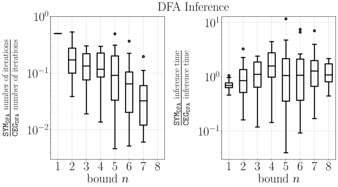
Figure 2: Comparison of SYM_DFA and CEG_DFA in terms of the runtime and the number of iterations of the main loop.

absence	existence	universality
$\operatorname{\mathbf{G}}(\lnot{a_{0}})$	$\operatorname{\mathbf{F}}{a_{0}}$	$\operatorname{\mathbf{G}}{a_{0}}$
$\operatorname{\mathbf{G}}(a_{1}\rightarrow{\operatorname{\mathbf{G}}(\lnot{a_{0}})})$	$(\operatorname{\mathbf{G}}(\lnot{a_{0}}))\lor(\operatorname{\mathbf{F}}(a_{0}\land(\operatorname{\mathbf{F}}{a_{1}})))$	$\operatorname{\mathbf{G}}(a_{1}\rightarrow{\operatorname{\mathbf{G}}{a_{0}}})$
$\operatorname{\mathbf{F}}{a_{1}}\rightarrow{(\lnot a_{0}\operatorname{\mathbf{U}}{a_{1}}})$	$\operatorname{\mathbf{G}}(a_{0}\land((\lnot{a_{1}})\rightarrow((\lnot{a_{1}})\operatorname{\mathbf{U}}(a_{2}\land(\lnot{a_{1}})))))$	$\operatorname{\mathbf{F}}{a_{1}}\rightarrow(a_{0}\operatorname{\mathbf{U}}{a_{1}})$
disjunction of common patterns
$(\operatorname{\mathbf{F}}{a_{2}})\lor((\operatorname{\mathbf{F}}{a_{0}})\lor(\operatorname{\mathbf{F}}{a_{1}}))$
$((\operatorname{\mathbf{G}}(\lnot{a_{0}}))\lor{(\operatorname{\mathbf{F}}(a_{0}\land(\operatorname{\mathbf{F}}{a_{1}}))))}\lor((\operatorname{\mathbf{G}}(\lnot{a_{3}}))\lor(\operatorname{\mathbf{F}}(a_{2}\land(\operatorname{\mathbf{F}}{a_{3}}))))$
$(\operatorname{\mathbf{G}}(a_{0}\land((\lnot{a_{1}})\rightarrow((\lnot{a_{1}})\operatorname{\mathbf{U}}(a_{2}\land(\lnot{a_{1}}))))))\lor(\operatorname{\mathbf{G}}(a_{3}\land((\lnot{a_{4}})\rightarrow((\lnot{a_{4}})\operatorname{\mathbf{U}}(a_{5}\land(\lnot{a_{4}}))))))$

Table 1: Common LTL patterns used for generation of words.

In S-SYM_LTL, we fixed the time horizon $K$ to a natural number, instead of the double exponential theoretical upper bound of $2^{2^{n+1}}$. Using this heuristic means that S-SYM_LTL does not solve Problem 2, but we demonstrate that we produced good enough formulas in practice.

In addition, we implemented two existing heuristics from Avellaneda and Petrenko (2018) to all the algorithms. First, in every algorithm, we learned models in an incremental manner, i.e., we started by learning DFAs (resp. LTL_f formulas) of size 1 and then increased the size by 1. We repeated the process until bound $n$. Second, we used a set of positive words $P^{\prime}$ instead of $P$ that starts as an empty set, and at each iteration of the algorithm, if the inferred language does not contain some words from $P$, we then extended $P^{\prime}$ with one of such words, preferably the shortest one. This last heuristic helped when dealing with large input samples because it used as few words as possible from the positive examples $P$.

We implemented every algorithm in Python 3, using PySAT (Ignatiev et al., 2018) for learning DFA, and an ASP (Baral, 2003) encoding that we solve using clingo (Gebser et al., 2017) for learning LTL_f formulas. Overall, we ran all the experiments using 8 GiB of RAM and two CPU cores with clock speed of 3.6 GHz.

5.0.1 Learning DFAs

For this case study, we considered a set of 28 random DFAs of size 2 to 10 generated using AALpy (Muškardin et al., 2022). Using each random DFA, we generated a set of 1000 positive words of lengths 1 to 10. We ran algorithms CEG_DFA and SYM_DFA with a timeout $TO=1000$s, and for $n$ up to 10.

Figure 2 shows a comparison between the performance of SYM_DFA and CEG_DFA in terms of the inference time and the required number of iterations of the main loop. On the left plot, the average ratio of the number of iterations is $0.14$, which, in fact, shows that SYM_DFA required noticeably less number of iterations compared to CEG_DFA. On the right plot, the average ratio of the inference time is $1.09$, which shows that the inference of the two algorithms is comparable, and yet SYM_DFA is computationally less expensive since it requires fewer iterations.

5.0.2 Learning Common LTL_f Patterns

In this case study, we generated sample words using 12 common LTL patterns (Dwyer et al., 1999), which we list in Table 1. Using each of these 12 ground truth LTL_f formulas, we generated a sample of 10000 positive words of length 10. Then, we inferred LTL_f formulas for each sample using CEG_LTL and S-SYM_LTL, separately. For both algorithms, we set the maximum formula size $n=10$ and a timeout of $TO=1000$s. For S-SYM_LTL, we additionally set the time horizon $K=8$.

Figure 3 represents a comparison between the mentioned algorithms in terms of inference time for the ground truth LTL_f formulas $\psi_{1}$, $\psi_{2}$, and $\psi_{3}$. On average, S-SYM_LTL ran 173.9% faster than CEG_LTL for all the 12 samples. Our results showed that the LTL_f formulas $\varphi$ inferred by S-SYM_LTL were more or equally specific than the ground truth LTL_f formulas $\psi$ (i.e., $\varphi\rightarrow\psi$) for five out of the 12 samples, while the LTL_f formulas $\varphi^{\prime}$ inferred by CEG_LTL were equally or more specific than the ground truth LTL_f formulas $\psi$ (i.e., $\varphi^{\prime}\rightarrow\psi$) for three out of the 12 samples.

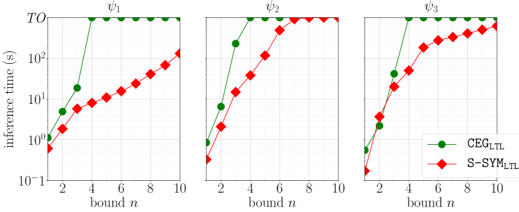
Figure 3: Comparison of S-SYM_LTL and CEG_LTL in terms of the inference time for three LTL ground truth formulas.

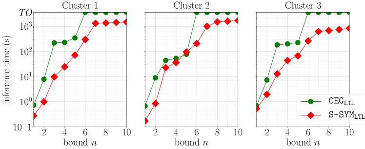
Figure 4: Comparison of S-SYM_LTL and CEG_LTL in terms of the runtime for three clusters of words taken from a UAV.

5.0.3 Learning LTL from Trajectories of Unmanned Aerial Vehicle (UAV)

In this case study, we implemented S-SYM_LTL and CEG_LTL using sample words of a simulated unmanned aerial vehicle (UAV) for learning LTL_f formulas. Here, we used 10000 words clustered into three bundles using the $k$-means clustering approach. Each word summarizes selective binary features such as $x_{0}$: “low battery”, $x_{1}$: “glide (not thrust)”, $x_{2}$: “change yaw angle”, $x_{3}$: “change roll angle”, etc. We set $n=10$, $K=8$, and a timeout of $TO=3600$s. We inferred LTL_f formulas for each cluster using CEG_LTL and S-SYM_LTL.

Figure 4 depicts a comparison between CEG_LTL and S-SYM_LTL in terms of the inference time for three clusters. Our results showed that, on average, S-SYM_LTL is 260.73% faster than CEG_LTL. Two examples of the inferred LTL_f formulas from the UAV words were $(\operatorname{\mathbf{F}}x_{1})\operatorname{\rightarrow}(\operatorname{\mathbf{G}}x_{1})$ which reads as “either the UAV always glides, or it never glides” and $\operatorname{\mathbf{G}}(x_{2}\operatorname{\rightarrow}{x_{3}})$ which reads as “a change in yaw angle is always accompanied by a change in roll angle”.

6 Conclusion

We presented novel algorithms for learning DFAs and LTL_f formulas from positive examples only. Our algorithms rely on conciseness and language minimality as regularizers to learn meaningful models. We demonstrated the efficacy of our algorithms in three case studies.

A natural direction of future work is to lift our techniques to tackle learning from positive examples for other finite state machines (e.g., non-deterministic finite automata) and more expressive temporal logics (e.g., linear dynamic logic (LDL) (Giacomo and Vardi, 2013)).

Appendix 0.A The Symbolic algorithm for learning DFAs with heuristics

We present the complete symbolic algorithm for learning DFAs along with the main heuristics (Problem 1). The pseudocode is sketched in Algorithm 4. Compared to the algorithm presented in Algorithm 1, we make a few modifications to improve performance. First, we introduce a set $P^{\prime}$ (also described in Section 5) to store the set of positive words necessary for learning the hypothesis DFA $\mathcal{A}^{\prime}$. Second, we incorporate an incremental DFA learning, meaning that we search for DFAs satisfying the propositional formula $\Phi^{\mathcal{A}}$ of increasing size (starting from size 1). To reflect this, we extend $\Phi^{\mathcal{A}}$ with the size parameter, represented using $\Phi^{\mathcal{A},m}$, to search for a DFA of size $m$.

Algorithm 4 Symbolic Algorithm for Learning DFA (with heuristics)

Input: Positive words $P$, bound $n$

1:  $\mathcal{A}\leftarrow\mathcal{A}_{\Sigma^{\ast}}$, $\Phi^{\mathcal{A}}\leftarrow\Phi_{\mathtt{DFA}}\wedge\Phi_{P}$

2:  $P^{\prime}\leftarrow\emptyset$, $m\leftarrow 1$

3:  while $m\leq n$ do

4:     $\Phi^{\mathcal{A},m}\leftarrow\Phi^{m}_{\mathtt{DFA}}\wedge\Phi_{P^{\prime}}\wedge\Phi_{\subseteq\mathcal{A}}\wedge\Phi_{\not\supseteq\mathcal{A}}$

5:     if no model $v$ satisfies $\Phi^{\mathcal{A},m}$ then

6:        $m\leftarrow m+1$

7:     else

8:        $\mathcal{A}^{\prime}\leftarrow$ DFA constructed from $v$

9:        if exists $w\in P\setminus L(\mathcal{A}^{\prime})$ then

10:           Add the shortest of such $w$ to $P^{\prime}$

11:        else

12:           $\mathcal{A}\leftarrow\mathcal{A}^{\prime}$

13:        end if

14:     end if

15:  end while

16:  return  $\mathcal{A}$

Appendix 0.B Comparison of Symbolic and Semi-symbolic Algorithm for Learning DFAs

We have introduced counterexample-guided, semi-symbolic and symbolic approaches in this paper. Our exploration of these methods will not be complete if we did not try a semi-symbolic algorithm for learning DFA. Hence, we introduce S-SYM_DFA, a semi-symbolic approach for learning DFA. This is done in a similar fashion than for LTL (Algorithm 2), but for DFA instead. Hence, we use the encoding $\Phi^{\mathcal{A}}\coloneqq\Phi_{\mathtt{DFA}}\wedge\Phi_{P}\wedge\Phi_{N}\wedge\Phi_{\not\supseteq\mathcal{A}}$. In practice, S-SYM_DFA is always worse than SYM_DFA, both in term of inference time (in average, $3.2$ times more) and number of iterations (in average, $2.1$ times more), as demonstrated in Figure 5.

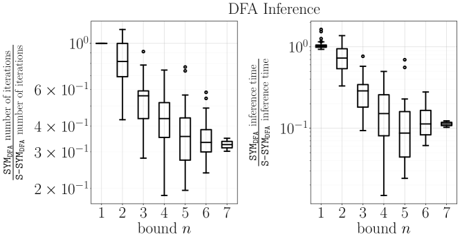
Figure 5: Comparison of SYM_DFA and S-SYM_DFA in terms of the inference time and the number of iterations of the main loop.

Appendix 0.C A Symbolic Algorithm for learning LTL formulas

We now describe few modifications to the semi-symbolic algorithm presented in Section 4.1 to convert it into a completely symbolic approach. This algorithm relies entirely on the hypothesis LTL formula $\varphi$ for constructing a propositional formula $\Psi^{\varphi}$ that guides the search of the next hypothesis. Precisely, the formula $\Psi^{\varphi}$ has the properties that: (1) $\Psi^{\varphi}$is satisfiable if and only if there exists an LTL formula $\varphi^{\prime}$ that is an $n\textrm{-description}$ and $\varphi\not\rightarrow\varphi^{\prime}$ and $\varphi^{\prime}\rightarrow\varphi$; and (2) based on a model $v$ of $\Psi^{\varphi,N}$, one can construct such an LTL formula.

The algorithm, sketched in Algorithm 5, follows the same framework as Algorithm 1. We here make necessary modifications to search for an LTL formula. Also, the propositional formula $\Psi^{\varphi}$ has a construction similar to $\Omega^{N,D}$, with the exception that $\Psi_{N}$ is replaced by $\Psi_{\rightarrow\varphi}$.

Algorithm 5 Symbolic Algorithm for Learning LTL

Input: Positive words $P$, bound $n$

1:  $\varphi\leftarrow\varphi_{\Sigma^{\ast}}$, $\Psi^{\varphi}\coloneqq\Psi_{\mathtt{LTL}}\wedge\Psi_{P}$

2:  while $\Psi^{\varphi}$ is satisfiable (with model $v$) do

3:     $\varphi\leftarrow$ LTL formula constructed from $v$

4:     $\Psi^{\varphi}\coloneqq\Psi_{\mathtt{LTL}}\wedge\Psi_{P}\wedge\Psi_{\rightarrow\varphi}\wedge\Psi_{\not\leftarrow\varphi}$

5:  end while

6:  return  $\varphi$

We here only describe the construction of the conjunct $\Psi_{\rightarrow\varphi}$ which reuses the variables and constraints already introduced in Section 4.1.

$$\Psi_{\rightarrow\varphi}\coloneqq\forall_{t\in[K],a\in{\Sigma}}p_{t,a}:\Big{[}\big{[}\Psi_{\mathtt{word}}\wedge\Psi_{\mathtt{sem}}\big{]}\rightarrow z^{\varphi^{\prime},n}_{w,t}\rightarrow z^{\varphi,n}_{w,t}\Big{]}$$ (27)

Intuitively, the above constraint says that if for all words $u$ of length $\leq K$, if $\varphi^{\prime}$ holds on $u$, then so must $\varphi$.

Appendix 0.D Evaluation of the Symbolic Algorithm for learning LTL formulas

We refer to this symbolic algorithm for learning LTL formulas (Algorithm 5) as SYM_LTL. We implement SYM_LTL using QASP2QBF Fandinno et al. (2021). SYM_LTL has an inference time several orders of magnitude above the inference time of S-SYM_LTL, as demonstrated in Figure 6. This can be explained by the choice of the solver, and the inherent complexity of the problem due to quantifiers. On the third experiment (Section 5.0.3), SYM_LTL timed out even for $n=1$.

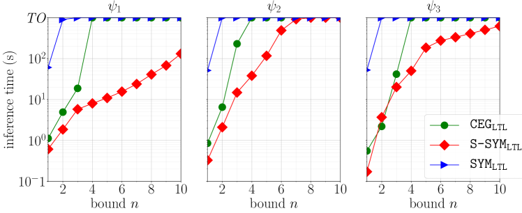
Figure 6: For each sample of the second experiment (Section 5.0.2), comparison of the inference time between CEG_LTL, S-SYM_LTL and SYM_LTL.

References

- Angluin (1980) Dana Angluin. Finding patterns common to a set of strings. Journal of Computer and System Sciences, 21(1):46–62, 1980. ISSN 0022-0000. doi: https://doi.org/10.1016/0022-0000(80)90041-0. URL https://www.sciencedirect.com/science/article/pii/0022000080900410.
- Avellaneda and Petrenko (2018) Florent Avellaneda and Alexandre Petrenko. Inferring DFA without negative examples. In Olgierd Unold, Witold Dyrka, and Wojciech Wieczorek, editors, Proceedings of the 14th International Conference on Grammatical Inference, ICGI 2018, Wrocław, Poland, September 5-7, 2018, volume 93 of Proceedings of Machine Learning Research, pages 17–29. PMLR, 2018. URL http://proceedings.mlr.press/v93/avellaneda19a.html.
- Baral (2003) Chitta Baral. Knowledge Representation, Reasoning and Declarative Problem Solving. Cambridge University Press, 2003. doi: 10.1017/CBO9780511543357.
- Biermann and Feldman (1972) Alan W. Biermann and Jerome A. Feldman. On the synthesis of finite-state machines from samples of their behavior. IEEE Trans. Computers, 21(6):592–597, 1972.
- Camacho and McIlraith (2019) Alberto Camacho and Sheila A. McIlraith. Learning interpretable models expressed in linear temporal logic. In ICAPS, pages 621–630. AAAI Press, 2019.
- Carrasco and Oncina (1999) Rafael C. Carrasco and José Oncina. Learning deterministic regular grammars from stochastic samples in polynomial time. RAIRO Theor. Informatics Appl., 33(1):1–20, 1999.
- Chou et al. (2022) Glen Chou, Necmiye Ozay, and Dmitry Berenson. Learning temporal logic formulas from suboptimal demonstrations: theory and experiments. Auton. Robots, 46(1):149–174, 2022.
- Dwyer et al. (1999) Matthew B. Dwyer, George S. Avrunin, and James C. Corbett. Patterns in property specifications for finite-state verification. In Barry W. Boehm, David Garlan, and Jeff Kramer, editors, Proceedings of the 1999 International Conference on Software Engineering, ICSE’ 99, Los Angeles, CA, USA, May 16-22, 1999, pages 411–420. ACM, 1999. doi: 10.1145/302405.302672. URL https://doi.org/10.1145/302405.302672.
- Ehlers et al. (2020) Rüdiger Ehlers, Ivan Gavran, and Daniel Neider. Learning properties in LTL ACTL from positive examples only. In FMCAD, pages 104–112. IEEE, 2020.
- Fandinno et al. (2021) Jorge Fandinno, François Laferrière, Javier Romero, Torsten Schaub, and Tran Cao Son. Planning with incomplete information in quantified answer set programming, 2021. URL https://arxiv.org/abs/2108.06405.
- Gebser et al. (2017) Martin Gebser, Roland Kaminski, Benjamin Kaufmann, and Torsten Schaub. Multi-shot ASP solving with clingo. CoRR, abs/1705.09811, 2017.
- Giacomo and Vardi (2013) Giuseppe De Giacomo and Moshe Y. Vardi. Linear temporal logic and linear dynamic logic on finite traces. In IJCAI, pages 854–860. IJCAI/AAAI, 2013.
- Giacomo and Vardi (2015) Giuseppe De Giacomo and Moshe Y. Vardi. Synthesis for LTL and LDL on finite traces. In IJCAI, pages 1558–1564. AAAI Press, 2015.
- Gold (1967) E. Mark Gold. Language identification in the limit. Inf. Control., 10(5):447–474, 1967.
- Gold (1978) E. Mark Gold. Complexity of automaton identification from given data. Inf. Control., 37(3):302–320, 1978.
- Grinchtein et al. (2006) Olga Grinchtein, Martin Leucker, and Nir Piterman. Inferring network invariants automatically. In IJCAR, volume 4130 of Lecture Notes in Computer Science, pages 483–497. Springer, 2006.
- Gunning et al. (2019) David Gunning, Mark Stefik, Jaesik Choi, Timothy Miller, Simone Stumpf, and Guang-Zhong Yang. Xai2014;explainable artificial intelligence. Science Robotics, 4(37):eaay7120, 2019. doi: 10.1126/scirobotics.aay7120. URL https://www.science.org/doi/abs/10.1126/scirobotics.aay7120.
- Hasanbeig et al. (2021) Mohammadhosein Hasanbeig, Natasha Yogananda Jeppu, Alessandro Abate, Tom Melham, and Daniel Kroening. Deepsynth: Automata synthesis for automatic task segmentation in deep reinforcement learning. In AAAI, pages 7647–7656. AAAI Press, 2021.
- Heule and Verwer (2010) Marijn Heule and Sicco Verwer. Exact DFA identification using SAT solvers. In 10th International Colloquium of Grammatical Inference: Theoretical Results and Applications, ICGI ’10, volume 6339 of LNCS, pages 66–79. Springer, 2010. doi: 10.1007/978-3-642-15488-1“˙7.
- Ignatiev et al. (2018) Alexey Ignatiev, Antonio Morgado, and Joao Marques-Silva. PySAT: A Python toolkit for prototyping with SAT oracles. In SAT, pages 428–437, 2018. doi: 10.1007/978-3-319-94144-8“˙26. URL https://doi.org/10.1007/978-3-319-94144-8“˙26.
- Jha et al. (2019) Susmit Jha, Ashish Tiwari, Sanjit A. Seshia, Tuhin Sahai, and Natarajan Shankar. Telex: learning signal temporal logic from positive examples using tightness metric. Formal Methods Syst. Des., 54(3):364–387, 2019. doi: 10.1007/s10703-019-00332-1. URL https://doi.org/10.1007/s10703-019-00332-1.
- Kasenberg and Scheutz (2017) Daniel Kasenberg and Matthias Scheutz. Interpretable apprenticeship learning with temporal logic specifications. In CDC, pages 4914–4921. IEEE, 2017.
- Lemieux et al. (2015) Caroline Lemieux, Dennis Park, and Ivan Beschastnikh. General LTL specification mining (T). In ASE, pages 81–92. IEEE Computer Society, 2015.
- Li and Manyà (2021) Chu-Min Li and Felip Manyà, editors. Theory and Applications of Satisfiability Testing - SAT 2021 - 24th International Conference, Barcelona, Spain, July 5-9, 2021, Proceedings, volume 12831 of Lecture Notes in Computer Science, 2021. Springer.
- Memarian et al. (2020) Farzan Memarian, Zhe Xu, Bo Wu, Min Wen, and Ufuk Topcu. Active task-inference-guided deep inverse reinforcement learning. In CDC, pages 1932–1938. IEEE, 2020.
- Molnar (2022) Christoph Molnar. Interpretable Machine Learning. 2 edition, 2022. URL https://christophm.github.io/interpretable-ml-book.
- Muškardin et al. (2022) Edi Muškardin, Bernhard Aichernig, Ingo Pill, Andrea Pferscher, and Martin Tappler. Aalpy: an active automata learning library. Innovations in Systems and Software Engineering, pages 1–10, 03 2022. doi: 10.1007/s11334-022-00449-3.
- Neider and Gavran (2018a) Daniel Neider and Ivan Gavran. Learning linear temporal properties. In Nikolaj Bjørner and Arie Gurfinkel, editors, 2018 Formal Methods in Computer Aided Design, FMCAD 2018, Austin, TX, USA, October 30 - November 2, 2018, pages 1–10. IEEE, 2018a. doi: 10.23919/FMCAD.2018.8603016. URL https://doi.org/10.23919/FMCAD.2018.8603016.
- Neider and Gavran (2018b) Daniel Neider and Ivan Gavran. Learning linear temporal properties, 2018b. URL https://arxiv.org/abs/1806.03953.
- Pnueli (1977) Amir Pnueli. The temporal logic of programs. In 18th Annual Symposium of Foundations of Computer Science, FOCS ’77, pages 46–57. IEEE Computer Society, 1977. doi: 10.1109/SFCS.1977.32. URL https://doi.org/10.1109/SFCS.1977.32.
- Rabin and Scott (1959) Michael Rabin and Dana Scott. Finite automata and their decision problems. IBM Journal of Research and Development, 3:114–125, 04 1959. doi: 10.1147/rd.32.0114.
- Raha et al. (2022) Ritam Raha, Rajarshi Roy, Nathanaël Fijalkow, and Daniel Neider. Scalable anytime algorithms for learning fragments of linear temporal logic. In TACAS (1), volume 13243 of Lecture Notes in Computer Science, pages 263–280. Springer, 2022.
- Roy et al. (2020) Rajarshi Roy, Dana Fisman, and Daniel Neider. Learning interpretable models in the property specification language. In IJCAI, pages 2213–2219. ijcai.org, 2020.
- Royal-Society (2019) Royal-Society. Explainable ai: The basics., 2019. URL ttps://royalsociety.org/-/media/policy/projects/explainable-ai/AI-and-interpretability-policy-briefing.pdf.
- Shvo et al. (2021) Maayan Shvo, Andrew C. Li, Rodrigo Toro Icarte, and Sheila A. McIlraith. Interpretable sequence classification via discrete optimization. In AAAI, pages 9647–9656. AAAI Press, 2021.
- Sistla and Clarke (1985) A. Prasad Sistla and Edmund M. Clarke. The complexity of propositional linear temporal logics. J. ACM, 32(3):733–749, 1985.
- Stern and Juba (2017) Roni Stern and Brendan Juba. Efficient, safe, and probably approximately complete learning of action models. In IJCAI, pages 4405–4411. ijcai.org, 2017.
- Stolcke and Omohundro (1992) Andreas Stolcke and Stephen Omohundro. Hidden markov model induction by bayesian model merging. In S. Hanson, J. Cowan, and C. Giles, editors, Advances in Neural Information Processing Systems, volume 5. Morgan-Kaufmann, 1992. URL https://proceedings.neurips.cc/paper/1992/file/5c04925674920eb58467fb52ce4ef728-Paper.pdf.
- Vazquez-Chanlatte et al. (2018) Marcell Vazquez-Chanlatte, Susmit Jha, Ashish Tiwari, Mark K. Ho, and Sanjit A. Seshia. Learning task specifications from demonstrations. In NeurIPS, pages 5372–5382, 2018.
- Weiss et al. (2018) Gail Weiss, Yoav Goldberg, and Eran Yahav. Extracting automata from recurrent neural networks using queries and counterexamples. In ICML, volume 80 of Proceedings of Machine Learning Research, pages 5244–5253. PMLR, 2018.
- Xu et al. (2019a) Zhe Xu, Alexander J Nettekoven, A. Agung Julius, and Ufuk Topcu. Graph temporal logic inference for classification and identification. In 2019 IEEE 58th Conference on Decision and Control (CDC), page 4761–4768. IEEE Press, 2019a. doi: 10.1109/CDC40024.2019.9029181. URL https://doi.org/10.1109/CDC40024.2019.9029181.
- Xu et al. (2019b) Zhe Xu, Melkior Ornik, A. Agung Julius, and Ufuk Topcu. Information-guided temporal logic inference with prior knowledge. In 2019 American Control Conference (ACC), pages 1891–1897, 2019b. doi: 10.23919/ACC.2019.8815145.
- Zhu et al. (2017) Shufang Zhu, Lucas M. Tabajara, Jianwen Li, Geguang Pu, and Moshe Y. Vardi. Symbolic ltlf synthesis. In IJCAI, pages 1362–1369. ijcai.org, 2017.