Unifying Generative Models with GFlowNets and Beyond

Abstract

There are many frameworks for deep generative modeling, each often presented with their own specific training algorithms and inference methods. Here, we demonstrate the connections between existing deep generative models and the recently introduced GFlowNet framework (Bengio et al., 2021b), a probabilistic inference machine which treats sampling as a decision-making process. This analysis sheds light on their overlapping traits and provides a unifying viewpoint through the lens of learning with Markovian trajectories. Our framework provides a means for unifying training and inference algorithms, and provides a route to shine a unifying light over many generative models. Beyond this, we provide a practical and experimentally verified recipe for improving generative modeling with insights from the GFlowNet perspective.

1 Introduction

Generative models are a class of machine learning algorithms that use probabilistic methods to capture and perform inference over complex distributions, usually from a given training dataset. They have a wide range of applications, including data generation, anomaly detection, probabilistic inference and density estimation. In the past few decades, a variety of different generative models have been developed, each with its own set of assumptions and capabilities.

Early examples of generative models include probabilistic graphical models, such as Bayesian networks and Markov random fields (Koller & Friedman, 2009; Murphy, 2012), and latent variable models, such as latent Dirichlet allocation (Blei et al., 2001) and Helmholtz machines (Dayan et al., 1995). These models have proven to be effective at capturing dependencies within data.

The research on generative modeling has taken off during the past decade, thanks to the representational power of deep neural networks. One well-known example is the generative adversarial network or GAN for short(Goodfellow et al., 2014), which consists of a generator network that stochastically produces new samples and a deterministic discriminator network that tries to distinguish between real and generated samples. Another popular method is the variational autoencoder (Kingma & Welling, 2013), which learns a hierarchical latent variable model to express the target distribution with the help of a variational posterior. Other types of generative models based on deep networks (deep generative models) include: normalizing flows (Dinh et al., 2014), which transform a simple distribution into a target distribution using a series of invertible transformations; autoregressive (AR) models (Bengio & Bengio, 1999; van den Oord et al., 2016), which model the distribution of a sequence of data by decomposing it into a product of conditional distributions; and energy-based models (Hinton, 2002; LeCun et al., 2006), which models the negative log probability of a distribution. Recently, denoising diffusion models (Vincent, 2011; Sohl-Dickstein et al., 2015; Ho et al., 2020; Song et al., 2020) have shown impressive results in generating high quality samples. Their modeling could be seen as a series of denoising steps which gradually transform white noise into noise-free data by stochastically inverting the process of transforming real data into white noise through a sequence of noise injection steps. Each of these generative models has its own set of assumptions and limitations, which can make it challenging to choose the right model for a particular task (Hu et al., 2018).

GFlowNets (Bengio et al., 2021a, b), short for generative flow networks, is a class of samplers which stems from a reinforcement learning or RL for short (Sutton & Barto, 2005) formulation. GFlowNets treat the sampling process as a sequential decision-making process, and learn a stochastic (forward) policy to sample compositional objects with probability proportional to a given terminating reward function. It has been demonstrated that GFlowNets are able to sample from diverse modes rather than being stuck in single modes like is typical of Markov chain Monte Carlo (MCMC) or variational inference methods (Zhang et al., 2022b; Malkin et al., 2023), which is of great importance in drug discovery (Jain et al., 2022a; Zhang et al., 2021).

In this paper, we show how many existing generative models could be taken as special cases of GFlowNets, with their modeling components specified in different probabilistic ways. We thus propose to treat the GFlowNet as a probabilistic framework for unifying different kinds of generative models, and facilitate the analysis of their connections and possible extensions (Section 3). Further, after analysing the relationship between GFlowNet setup and generative modeling setup in Section 4, we propose MLE-GFN, a generative modeling algorithm inspired by GFlowNet ideas in Section 5. The proposed algorithm improves the performances of existing generative modeling baselines on both discrete and continuous image modeling tasks.

2 Preliminaries and Notations

2.1 Generative Modeling

Generative modeling aims to use probabilistic methods to model a distribution from a given dataset $\mathfrak{D}=\{\mathbf{x}_{i}\}_{i},\mathbf{x}_{i}\in\mathcal{X}$, where $\mathcal{X}$ is the space of data objects. When considering the training task, we want to learn a distribution $q(\mathbf{x})$ to be close to the target distribution $p^{*}(\mathbf{x})=\frac{1}{|\mathfrak{D}|}\sum_{i}\delta_{\{\mathbf{x}_{i}-\mathbf{x}\}}$, where $\delta_{\{\cdot\}}$ is the Dirac distribution. However, the real objective is to generalize well to an underlying data generating process $p^{*}$ from which both training samples and test samples may be drawn. One example to achieve this is to minimize the KL divergence, i.e., $\min_{q}\mathcal{D}_{\mathrm{KL}}\left(p^{*}\|q\right)$, which corresponds to the maximum likelihood estimation (MLE), a popular method for training generative models. Other methods could also be taken as examples of divergence minimization, e.g., GAN’s adversarial training could be viewed as minimizing the Jensen-Shannon divergence between the model and the target distribution.

2.2 GFlowNets

From a probabilistic modeling viewpoint, a generative flow network (GFlowNet) (Bengio et al., 2021a, b) is a probabilistic inference methodology that aims to sample $\mathbf{x}\in\mathcal{X}$ in proportion to a given reward function $R(\mathbf{x})$, where $\mathcal{X}$ is the set of data. That is to say, the target distribution $p^{*}(\cdot)$ that we want so sample from satisfies $p^{*}(\mathbf{x})\propto R(\mathbf{x})$. Recently, the community has experienced a progressive expansion of the concept of GFlowNets (Malkin et al., 2022; Deleu et al., 2022; Jain et al., 2022a, b; Pan et al., 2022; Madan et al., 2022; Liu et al., 2022). More precisely, a GFlowNet samples a Markovian trajectory $\tau=(\mathbf{s}_{0},\mathbf{s}_{1},\ldots,\mathbf{s}_{n})$ with length $n+1$, where $\mathbf{s}_{i}\in\mathcal{S}$ is the intermediate states for all $i$ in $[n]:=\{0,1,\ldots,n\}$, whose space $\mathcal{S}$ is not necessarily the same as $\mathcal{X}$. If not specially specified, we use the notation $\mathbf{x}=\mathbf{s}_{n}$ for the final / terminating state of the trajectory. This process has a natural connection to reinforcement learning (Sutton & Barto, 2005; Bengio et al., 2021a; Zhang et al., 2022a). The set of all trajectories $\tau$ form a directed acyclic graph (DAG) in the latent state space, whose nodes are states $\mathbf{s}\in\mathcal{S}$. Each complete trajectory starts from the same (abstract) initial state $\mathbf{s}_{0}$ and ends in a terminating state $\mathbf{s}_{n}$. The flow function $F(\tau)\in\mathbb{R}_{+}$ defined by Bengio et al. (2021b) can be understood by an analogy with the number of water particles flowing through trajectory $\tau$ in a network of pipes with $s_{0}$ as single source and all the terminating states as sinks. Ideally, we want the amount of flow leading to $\mathbf{x}$ equals the given reward: $\sum_{\tau=(\mathbf{s}_{0},\cdots,\mathbf{s}_{n}),\mathbf{s}_{n}=\mathbf{x}}F(\tau)=R(\mathbf{x})$.

Several training criteria have already been proposed for GFlowNets. We start from the flow matching condition (Equation 1). Define $F(\mathbf{s},\mathbf{s}^{\prime})\triangleq\sum_{(\mathbf{s}\to\mathbf{s}^{\prime})\in\tau}F(\tau)$ as the edge flow function and $F(\mathbf{s})\triangleq\sum_{\mathbf{s}\in\tau}F(\tau)$ as the state flow function. It is easy to see that the incoming flow into $\mathbf{s}^{\prime}$ should match the outgoing flow from $\mathbf{s}^{\prime}$:

$$\sum_{\mathbf{s},\mathbf{s}\to\mathbf{s}^{\prime}}F(\mathbf{s},\mathbf{s}^{\prime})=\sum_{\mathbf{s}^{\prime\prime},\mathbf{s}^{\prime}\to\mathbf{s}^{\prime\prime}}F(\mathbf{s}^{\prime},\mathbf{s}^{\prime\prime}),$$ (1)

as both side of the equation must equal $F(\mathbf{s}^{\prime})$. If one parametrizes the GFlowNet with the edge flow function $F_{\theta}(\cdot,\cdot)$, then the constraint in Equation 1 would be used to define a corresponding training loss (i.e., $\mathcal{L}({\boldsymbol{\theta}},\mathbf{s}^{\prime})=\left(\log\sum_{\mathbf{s}}F_{{\boldsymbol{\theta}}}(\mathbf{s},\mathbf{s}^{\prime})-\log\sum_{\mathbf{s}^{\prime\prime}}F_{{\boldsymbol{\theta}}}(\mathbf{s}^{\prime},\mathbf{s}^{\prime\prime})\right)^{2}$), such that when the loss is zero everywhere, the constraint is satisfied, and 0 is also a global minimum of the loss.

The detailed balance constraint of GFlowNets writes

$$F(\mathbf{s})P_{F}\left(\mathbf{s}^{\prime}\mid\mathbf{s}\right)=F(\mathbf{s}^{\prime})P_{B}\left(\mathbf{s}\mid\mathbf{s}^{\prime}\right),$$ (2)

where $P_{F}(\mathbf{s}^{\prime}|\mathbf{s})$ and $P_{B}(\mathbf{s}|\mathbf{s}^{\prime})$ are referred to as the forward and backward policy respectively and characterize the stochastic transitions between different states, going forward or backward along a trajectory. We can separately parametrize three models for $F_{\boldsymbol{\theta}}(\cdot),P_{F}(\cdot|\cdot;{\boldsymbol{\theta}}),P_{B}(\cdot|\cdot;{\boldsymbol{\theta}})$. The detailed balance condition is closely related to the flow matching condition, in the sense that $P_{F}(\mathbf{s}^{\prime}|\mathbf{s})={F(\mathbf{s},\mathbf{s}^{\prime})}/{F(\mathbf{s})}$ and $P_{B}(\mathbf{s}|\mathbf{s}^{\prime})=F(\mathbf{s},\mathbf{s}^{\prime})/F(\mathbf{s}^{\prime})$. to determine a GFlowNet, it suffices to specify its forward policy (Bengio et al., 2021b).

Extending the detailed balance criterion to a constraint on the whole trajectory, the (general) trajectory balance criterion (Malkin et al., 2022) of GFlowNets aims to match GFlowNet’s forward trajectory probability $P_{F}(\tau)$ and the backward trajectory probability $P_{B}(\tau)$, where

$$P_{F}(\tau) =\prod_{i=0}^{n-1}P_{F}\left(\mathbf{s}_{i+1}|\mathbf{s}_{i}\right)$$ (3)

$$P_{B}(\tau) =\frac{R\left(\mathbf{x}\right)}{Z}\prod_{t=0}^{n-1}P_{B}\left(\mathbf{s}_{i}|\mathbf{s}_{i+1}\right),$$ (4)

where $\mathbf{x}=\mathbf{s}_{n}$. Notice that $\mathbf{s}_{0}$ is defined to be an abstract initial state (i.e., the first state of any trajectory) which has no concrete meaning for formalization reasons (Bengio et al., 2021b). Here $Z=\sum_{\mathbf{x}}R(\mathbf{x})$ is the normalizing factor which generally needs to be learned (and can then be included in the overall parameter vector $\theta$). We also note that $P_{B}(\tau|\mathbf{x})=\prod_{i=0}^{n-1}P_{B}\left(\mathbf{s}_{i}\mid\mathbf{s}_{i+1}\right)$ when $\mathbf{x}$ is the terminating state of the trajectory $\tau$. Concretely, Malkin et al. (2022) proposes to use $(\log P_{F}(\tau)-\log P_{B}(\tau))^{2}$ as a training objective; nonetheless, in this work we focus on general divergences between the two distributions (e.g., KL divergence; we call such specification KL-trajectory balance). We also use $P_{T}(\mathbf{x})=\sum_{\tau=(\mathbf{s}_{0},\cdots,\mathbf{s}_{n}),\mathbf{s}_{n}=\mathbf{x}}P(\tau)$ to denote the terminating distribution, namely the distribution on $\mathcal{X}$ that GFlowNet could generate.

Continuous GFlowNets.

Lahlou et al. (2023) developed a theory for GFlowNets with continuous or hybrid states, generalizing that for discrete states. In short, this theory allows one to use the same GFlowNet losses as in the discrete case, but replacing probability masses, such as $P_{F}(\mathbf{s}^{\prime}|\mathbf{s})$, by probability density functions $p_{F}(\mathbf{s}^{\prime}|\mathbf{s})$ as required, so long as all p.d.f.s are expressed in a compatible way, i.e., with respect to a common reference measure. In this paper, we are concerned with sampling in Euclidean spaces and will thus use $P_{F}$, $P_{B}$ interchangeably with their densities with respect to the Lebesgue measure on $\mathbb{R}^{n}$.

3 GFlowNet as a Unifying Framework

3.1 Hierarchical Variational Autoencoders

The evidence lower bound for bottom-up hierarchical VAEs (HVAEs) (Ranganath et al., 2016) reads

$$\log p(\mathbf{x})\geq\textrm{ELBO}_{p,q}(\mathbf{x})$$ (5)

$$\triangleq\mathbb{E}_{q(\mathbf{z}_{1:n-1}|\mathbf{x})}\left[\log p(\mathbf{x},\mathbf{z}_{1:n-1})-\log q(\mathbf{z}_{1:n-1}|\mathbf{x})\right]$$ (6)

$$=\mathop{\mathbb{E}}_{q(\mathbf{z}_{n-1}|\mathbf{z}_{n})\cdots q(\mathbf{z}_{1}|\mathbf{z}_{2})}\left[\log p(\mathbf{z}_{1})+\sum_{i=1}^{n-1}\log\frac{p(\mathbf{z}_{i+1}|\mathbf{z}_{i})}{q(\mathbf{z}_{i}|\mathbf{z}_{i+1})}\right],$$ (7)

where we denote $\mathbf{x}:=\mathbf{z}_{n}$, $\mathbf{z}_{1:n-1}=(\mathbf{z}_{1},\ldots,\mathbf{z}_{n-1})$, and $p,q$ respectively denote the hierarchical decoder and encoder of the HVAE. It is well known that this hierarchical ELBO can also be represented as $\mathcal{D}_{\mathrm{KL}}\left(q(\mathbf{z}_{1:n-1}|\mathbf{x})\|p(\mathbf{z}_{1:n-1}|\mathbf{x})\right),$ where $p(\mathbf{z}_{1:n-1}|\mathbf{x})\propto p(\mathbf{x}|\mathbf{z}_{1:n-1})p(\mathbf{z}_{1:n-1})$. As we show below, with a GFlowNet that samples $\mathbf{z}$ given $\mathbf{x}$ and where the reward is $p(\mathbf{x},\mathbf{z}_{1:n-1})$, we also aim to match the forward trajectory policy which ends with data $\mathbf{x}$ with the corresponding backward trajectory policy, i.e., $P_{F}(\tau)\approx P_{B}(\tau)$, conditioning on the event $\{\mathbf{x}\in\tau\}$, i.e., $\mathbf{x}$ is the terminating state of $\tau$. Note that we have $\mathbb{P}(\mathbf{x}|\tau)=\delta_{\{\mathbf{x}\in\tau\}}$, where $\mathbb{P}(\cdot)$ denotes the probability of some event.

Observation 1.

The HVAE is a special kind of GFlowNet in the following sense: each trajectory is of the form of $\tau=(\mathbf{z}_{0},\mathbf{z}_{1},\cdots,\mathbf{z}_{n}=\mathbf{x})$. The VAE decoder, which samples $\mathbf{z}_{0}\to\cdots\to\mathbf{z}_{n-1}\to\mathbf{z}_{n}$, corresponds to the GFlowNet forward policy; the encoder samples $\mathbf{x}\to\mathbf{z}_{n-1}\to\cdots\to\mathbf{z}_{0}$, and corresponds to the GFlowNet backward policy.

With $\mathbf{x}=\mathbf{z}_{n}$, we could then write

$$P_{F}(\tau)=p(\mathbf{z}_{0})\prod_{i=1}^{n-1}p(\mathbf{z}_{i+1}|\mathbf{z}_{i}),$$ (8)

$$P_{B}(\tau)=p^{*}(\mathbf{x})\prod_{i=1}^{n-1}q(\mathbf{z}_{i}|\mathbf{z}_{i+1}),$$ (9)

where $p^{*}(\mathbf{x})=\frac{R(\mathbf{x})}{Z}$ is the true target density, $p(\cdot|\cdot)$ is the forward policy, and $q(\cdot|\cdot)$ is the backward policy. We can see that the $i$-th state in a GFlowNet trajectory (i.e., $\mathbf{s}_{i}$) corresponds to $\mathbf{z}_{i}$.

The following proposition reveals an equivalence between the two perspectives in Observation 1.

Proposition 2.

Training hierarchical latent variable models with the KL-trajectory balance $\mathcal{D}_{\mathrm{KL}}\left(P_{B}(\tau)\|P_{F}(\tau)\right)$ objective is equivalent to training HVAEs by maximizing its ELBO, in the sense of having the same global optimum.

In this work we relegate all proofs to Section B. We refer to Sønderby et al. (2016); Child (2021); Shu & Ermon (2022) for practice of HVAEs on large scale image modeling.

3.2 Diffusion Models

3.2.1 Denoising diffusion probabilistic models

The success of deep learning relies on careful design of inductive biases in the learning algorithm (Goyal & Bengio, 2020). With the same amount of computational resources and data, the better assumptions we use to constrain the model, the more powerful and better generalizing the algorithm will be. One way to bake inductive biases into the aforementioned hierarchical VAE model is by forcing the following Gaussian assumptions:

$$P_{F}(\mathbf{s}_{i+1}|\mathbf{s}_{i}) =\mathcal{N}(\mathbf{s}_{i+1};\boldsymbol{\mu}_{i}(\mathbf{s}_{i}),\beta_{i}\mathbf{I}),$$ (10)

$$P_{B}(\mathbf{s}_{i}|\mathbf{s}_{i+1}) =\mathcal{N}(\mathbf{s}_{i};\sqrt{1-\beta_{i}}\mathbf{s}_{i+1},\beta_{i}\mathbf{I}),$$ (11)

where $i=0,\ldots,n-1$ are integer indices, $\mathcal{N}$ denotes the Gaussian distribution, $\{\mu_{i}(\cdot)\}_{i}$ are functions to be learned, and $\{\beta_{i}\}_{i}$ are constant positive real numbers. In this way, the latent variables at every stage of the sequential generative process share the same number of dimensions as data $\mathbf{x}$.

Observation 3.

The denoising diffusion probabilistic model or DDPM for short (Ho et al., 2020) is a special kind of GFlowNet with the forward policy specified as in Equation 10 and the backward policy specified as in  Equation 11.

Remark that our notation of the time index is in the reverse ordering of the one used in the DDPM exposition, which results in a slightly different definition of $\beta$. With the special design in Equation 10 and  11, a DDPM enjoys an efficient training procedure (each $\boldsymbol{\mu}_{i}$ can be trained locally by only trying to invert the noise added to $s_{i+1}$ to obtain $s_{i}$), which helps it scale well and made it become a state-of-the-art method for high-dimensional image generative modeling (Dhariwal & Nichol, 2021; Kingma et al., 2021). We analyze the relationship between its training objective and a GFlowNet formulation in the following proposition.

Proposition 4 (informal).

Training a GFlowNet defined as in Equation 10 and  11 with KL-trajectory balance is equivalent to training a DDPM with its regression-based denoising objective.

Discrete space diffusion

The above modeling method could also generalize to structured discrete data. For categorical (i.e., discrete) data, $\mathbf{s}_{i}$ denotes the one-hot representation of $\mathbf{s}_{i}$, and we define a hierarchical model as in Section 3.1 in the manner of the following claim, which parallels Observation 3:

Observation 5.

The discrete denoised diffusion model for categorical data proposed by Hoogeboom et al. (2021); Austin et al. (2021) is a special case of GFlowNet with the forward policy specified in Equation 12 and backward policy specified in Equation 13.

$$P_{F}(\mathbf{s}_{i+1}|\mathbf{s}_{i}) =\mathcal{C}(\mathbf{s}_{i+1};\mathbf{p}=\boldsymbol{\mu}_{i}(\mathbf{s}_{i})),$$ (12)

$$P_{B}(\mathbf{s}_{i}|\mathbf{s}_{i+1}) =\mathcal{C}(\mathbf{s}_{i};\mathbf{p}=\mathbf{s}_{i+1}\mathbf{Q}_{i}),$$ (13)

where $\mathcal{C}$ denotes a categorical distribution, $\{\mathbf{Q}_{i}\}_{i}$ are doubly-stochastic constant Markov transition matrices, and $\{\boldsymbol{\mu}_{i}(\cdot)\}_{i}$ are parametric functions serving as the categorical parameter for the GFlowNet forward policy.

3.2.2 Denoised diffusion through SDEs

The behavior of a deep latent variable model in its infinite depth regime is studied by Tzen & Raginsky (2019); in the language of GFlowNets, the forward and backward policy take the following form:

$$P_{F}(\mathbf{s}_{i+1}|\mathbf{s}_{i}) =\mathcal{N}\left(\mathbf{s}_{i+1};\mathbf{s}_{i}+h\mathbf{f}_{i}(\mathbf{s}_{i}),hg^{2}_{i})\right),$$ (14)

$$P_{B}(\mathbf{s}_{i}|\mathbf{s}_{i+1}) =\mathcal{N}(\mathbf{s}_{i};\mathbf{s}_{i+1}+h\large(-\mathbf{f}_{i+1}(\mathbf{s}_{i+1})$$ (15)

$$\quad\quad+g^{2}_{i+1}\nabla\log F(\mathbf{s}_{i+1})\large),hg^{2}_{i+1}),$$ (16)

where we assume all $\mathbf{s}_{i}$ have the same number of dimensions as $\mathbf{x}$, time step $h=1/L$, $\{g_{i}\}_{i}$ are scalar parameters, and $\{\mathbf{f}_{i}(\cdot):\mathcal{S}\to\mathcal{S}\}_{i}$ are parametric mappings. The hierarchical model is then equivalent to a stochastic process in its diffusion limit ( $h\to 0$). Huang et al. (2021); Kingma et al. (2021); Song et al. (2021) also study connections between hierarchical variational inference on deep latent variable models and diffusion processes.

Consider a stochastic differential equation (SDE) (Øksendal, 1985) and its reverse time SDE (Anderson, 1982)

$$\mathop{}\!\mathrm{d}\mathbf{x} =\mathbf{f}(\mathbf{x})\mathop{}\!\mathrm{d}t+g(t)\mathop{}\!\mathrm{d}\mathbf{w}_{t},$$ (17)

$$\mathop{}\!\mathrm{d}\bar{\mathbf{x}} =\left[\mathbf{f}(\bar{\mathbf{x}})-g^{2}(t)\nabla_{\bar{\mathbf{x}}}\log p_{t}(\bar{\mathbf{x}})\right]\mathop{}\!\mathrm{d}\bar{t}+g(t)\mathop{}\!\mathrm{d}\bar{\mathbf{w}}_{t},$$ (18)

where $\mathbf{f}(\cdot)$ and $g(\cdot)$ are given and $\mathbf{x},\mathbf{w}\in\mathbb{R}^{D}$, $\mathop{}\!\mathrm{d}\mathbf{w}_{t}$ is a Wiener process, and $\bar{\mathbf{x}},\bar{t},\bar{\mathbf{w}}_{t}$ denote the reverse time version of $\mathbf{x},t,\mathbf{w}_{t}$. We define $\mathbb{P}_{h}(\mathbf{x}_{t+h}|\mathbf{x}_{t})$ to be the transition kernel induced by the SDE in Equation 17, namely $\mathbf{x}_{t+h}=\mathbf{x}_{t}+\int_{t}^{t+h}f(\mathbf{x}_{\tau})\mathop{}\!\mathrm{d}\tau+\int_{t}^{t+h}g(\tau)\mathop{}\!\mathrm{d}\mathbf{w}_{\tau}$, where $h$ denotes an infinitesimal time step. This modeling, adopted and popularized by Song et al. (2020, ScoreSDE), could be connected to GFlowNets as follows.

Observation 6.

ScoreSDE is a special case of GFlowNets, in the sense that GFlowNet states take the time-augmented form $\mathbf{s}_{t}=(\mathbf{x}_{t},t)$ for some $t\in[0,1]$, the SDE in Equation 17 models the forward policy of GFlowNets (i.e., how states should move forward) while the reverse time SDE in Equation 18 models the backward policy of GFlowNets (i.e., how states should move backward). In this case, a trajectory $\{\mathbf{s}_{t}\}_{t=0}^{1}$ is also in the form of $\{\mathbf{x}_{t}\}_{t=0}^{1}$.

Note that we cannot directly treat $\mathbf{x}_{t}$ to be a GFlowNet state, as the theory of GFlowNets requires the graph of all latent states to be a DAG (i.e., one cannot return to an already visited state). This state augmenting operation (Bengio et al., 2021b) induces the required DAGness, including in the SDE case. This follows because any $(\mathbf{x},t)\to(\mathbf{x}^{\prime},t^{\prime})$ transition with $t\geq t^{\prime}$ is forbidden. Without loss of generality, we assume that the notation $\mathbf{x}_{t}$ as a GFlowNet state already contains the time stamp itself in the context below.

We now point out an analogy between a stochastic processes property and a GFlowNet property:

Observation 7.

The property of a stochastic process

$$\int p(\mathbf{x}_{t-h},t-h)\mathbb{P}_{h}(\mathbf{x}_{t}|\mathbf{x}_{t-h})\mathop{}\!\mathrm{d}\mathbf{x}_{t-h}$$ (19)

$$\quad=\int p(\mathbf{x}_{t},t)\mathbb{P}_{h}(\mathbf{x}_{t+h}|\mathbf{x}_{t})\mathop{}\!\mathrm{d}\mathbf{x}_{t+h}=p(\mathbf{x}_{t},t),$$

can be interpreted as the GFlowNets flow matching constraint

$$\sum_{\mathbf{s}}F(\mathbf{s},\mathbf{s}^{\prime})=\sum_{\mathbf{s}{{}^{\prime\prime}}}F(\mathbf{s}^{\prime},\mathbf{s}{{}^{\prime\prime}})\triangleq F(\mathbf{s}^{\prime}),\ \forall\mathbf{s}^{\prime}\in\mathcal{S},$$ (20)

where we have $F(\mathbf{s},\mathbf{s}^{\prime})=F(\mathbf{s})P_{F}(\mathbf{s}^{\prime}|\mathbf{s})$.

We point out that Equation LABEL:eq:diffusion_markov is a standard starting point for deriving the Fokker-Planck equation, as shown in Appendix:

Proposition 8 (Øksendal (1985)).

Taking the limit as $h\rightarrow 0$, Equation LABEL:eq:diffusion_markov implies

$$\begin{split}\partial_{t}p(\mathbf{x},t)=-\nabla_{\mathbf{x}}&\left(p(\mathbf{x},t)\mathbf{f}(\mathbf{x},t)\right)\\ &+\frac{1}{2}\nabla_{\mathbf{x}}^{2}\left(p(\mathbf{x},t)g^{2}(\mathbf{x},t)\right).\end{split}$$ (21)

Equivalence between detailed balance and score matching. We investigate such a setting where we want to model the reverse process:

$$\mathop{}\!\mathrm{d}\mathbf{x} =\left[\mathbf{f}(\mathbf{x})-g^{2}(t)\mathbf{s}(\mathbf{x},t)\right]\mathop{}\!\mathrm{d}\bar{t}+g(t)\mathop{}\!\mathrm{d}\bar{\mathbf{w}}_{t},$$ (22)

where $\mathbf{s}(\cdot,\cdot):\mathbb{R}^{D}\times[0,1]\to\mathbb{R}^{D}$ is a neural network, and $\mathbf{f}(\cdot)$ and $g(\cdot)$ are given. We propose to use the detailed balance criterion of GFlowNets to learn this neural network. From the above discussion, we can see there is an analogy realized by $F(\mathbf{s}_{t})\approx p_{t}(\mathbf{x})$. We show the validity of such a strategy in the following proposition.

Proposition 9.

GFlowNets’ detailed balance condition

$$\begin{split}&\lim_{h\rightarrow 0}\frac{1}{\sqrt{h}}\huge(\log p_{t}(\mathbf{x}_{t})+\log P_{F}(\mathbf{x}_{t+h}|\mathbf{x}_{t})-\\ &\quad\log p_{t+h}(\mathbf{x}_{t+h})+\log P_{B}(\mathbf{x}_{t}|\mathbf{x}_{t+h})\huge)=0,\end{split}$$ (23)

$(\forall\mathbf{x}_{t}\in\mathbb{R}^{D},\forall t\in(0,1))$ is equivalent to

$${\boldsymbol{\epsilon}}^{\top}\left(\mathbf{s}(\mathbf{x}_{t},t)-\nabla_{\mathbf{x}}\log p_{t}(\mathbf{x})\right)=0,\forall{\boldsymbol{\epsilon}},\mathbf{x}_{t}\in\mathbb{R}^{D},\forall t\in[0,1],$$

which is the optimal solution to (sliced) score matching:

$$\min_{\mathbf{s}}\mathbb{E}_{\mathbf{x}\sim p_{t}}\mathbb{E}_{\boldsymbol{\epsilon}}\left[{\boldsymbol{\epsilon}}^{\top}\nabla_{\mathbf{x}}\mathbf{s}(\mathbf{x}){\boldsymbol{\epsilon}}+\frac{1}{2}\left({\boldsymbol{\epsilon}}^{\top}\mathbf{s}(\mathbf{x},t)\right)^{2}\right],\forall t.$$

3.2.3 Schrödinger Bridge

The Schrödinger Bridge or SB for short (Schrödinger, 1932; Léonard, 2013; Chen et al., 2021) is a classical problem which solves the entropy regularized optimal transport. In order to achieve this bridging target, the Iterative Proportional Fitting or IPF for short (Kullback, 1968) method proposes to solve the Schrödinger Bridge problem with the following alternating optimization:

$$\pi^{2m+1} =\operatorname*{arg\,min}\{\mathcal{D}_{\mathrm{KL}}\left(\pi\|\pi^{2m}\right):\pi_{\text{start}}=p_{\text{prior}}\},$$ (24)

$$\pi^{2m+2} =\operatorname*{arg\,min}\{\mathcal{D}_{\mathrm{KL}}\left(\pi\|\pi^{2m+1}\right):\pi_{\text{end}}=p^{*}\},$$ (25)

where $\pi,\pi^{m}\in\mathcal{P}(\mathcal{X}^{n+1})$, namely distributions on $\mathcal{X}^{n+1}$ space, $\pi^{0}$ is initialized to some given base measure, and $\pi_{\text{start}},\pi_{\text{end}}\in\mathcal{P}(\mathcal{X})$ refer to the marginal distribution of $\pi$ on the first and last index respectively.

In practice, IPF models the joint distribution $\pi$ in Equation 24 in the decomposition form of forward probability product $\pi_{\text{start}}(\mathbf{s}_{1})\prod_{i}p(\mathbf{s}_{i+1}|\mathbf{s}_{i})$, as in Equation 8 and 10, as the marginal distribution on the first state is fixed. On the contrary, $\pi$ in Equation 25 is modelled with backward probability decomposition $\pi_{\text{end}}(\mathbf{s}_{n})\prod_{i}p(\mathbf{s}_{i}|\mathbf{s}_{i+1})$, as in Equation 9 and 11. As a matter of fact, such a discrete-time SB formulation generalizes the DDPM by relaxing the constraint on its noise diffusion process.

Observation 10.

The discrete-time Schrödinger Bridge is a special case of GFlowNet. Compared to the DDPM formulation, SB does not use a fixed backward policy, but learns both the forward and backward policies together.

We remark that such alternating optimization is in the same spirit as the wake-sleep algorithm (Hinton et al., 1995) for learning latent variable models without requiring something like the REINFORCE gradient estimator. Regarding the continuous-time setup, a similar observation could be made that SB generalizes the ScoreSDE formulation by not using a fixed noising process. We refer to Bortoli et al. (2021); Shi et al. (2022) for practical guidance regarding learning diffusion SB for generative modeling.

3.3 Exact Likelihood Models

Autoregressive (AR) models can b e viewed as sampling $p(\mathbf{x}_{1:i+1}|\mathbf{x}_{1:i})$ sequentially one dimension $i$ at a time in order to generate the final vector $\mathbf{x}$. Zhang et al. (2022b) use an AR-like (with a learnable ordering) model to parametrize the GFlowNet. Indeed, we can define every (forward) action of the GFlowNet as specifying one more pixel on top of the current state, and the backward policy turns one pixel into an unspecified value (Zhang et al., 2022b). This makes AR models special cases of GFlowNet where the order in which the pixels are specified is fixed, making the GFlowNet DAG a tree (Bengio et al., 2021a).

Observation 11.

The standard autoregressive model is a special kind of GFlowNet where

• $\mathbf{s}_{i}:=\mathbf{x}_{1:i}$ is the GFlowNet state;

• $P_{F}(\mathbf{s}_{i+1}|\mathbf{s}_{i})=p(\mathbf{x}_{1:i+1}|\mathbf{x}_{1:i})$ is the forward policy;

• $P_{B}(\mathbf{s}_{i}|\mathbf{s}_{i+1})=\delta\{\mathbf{s}_{i}\ \textrm{comprises the first}\ i\text{ dimensions of}\ \mathbf{s}_{i+1}\}$,

where $\delta\{\cdot\}$ is the Dirac Delta distribution for continuous variables, and is the indicator function in the discrete case.

This modeling makes the latent graph of the GFlowNet to be a tree; alternatively, if we allow a learnable ordering as with Zhang et al. (2022b), the trajectories in latent space form a general DAG. This is related to non-autoregressive modeling methods in the NLP community (Gu et al., 2018).

The normalizing flow or NF for short (Dinh et al., 2015) is another way to sequentially construct desired data. It first samples $\mathbf{z}_{1}$ from a base distribution (usually the standard Gaussian), and then applies a series of invertible transformations $\mathbf{z}_{i+1}=\mathbf{f}(\mathbf{z}_{i})$ until one finally obtains $\mathbf{x}:=\mathbf{z}_{n}$, where $n$ denotes the number of transformation layers.

Observation 12.

The NF is a special kind of GFlowNet with deterministic forward and backward policies (except the first transition step), and $\mathbf{s}_{i}=\mathbf{z}_{i}$ are GFlowNet states.

With the GFlowNet implementation of NF, the base distribution is the first (and only stochastic) step, while the other steps are deterministic. When both $P_{F}(\mathbf{z}_{i+1}|\mathbf{z}_{i})$ and $P_{B}(\mathbf{z}_{i}|\mathbf{z}_{i+1})$ are deterministic (each being a Dirac at the value of some function applied to the conditioning argument) and match each other, it must be that they correspond to invertible functions. We next discuss maximum likelihood estimation (MLE) of AR and NF models.

About MLE training. AR models and NFs are usually trained with MLE. Although the likelihood of general GFlowNets is intractable, we lower bound it:

$$\log p_{T}(\mathbf{x}) =\int_{\mathbf{x}\in\tau}P_{F}(\tau)\mathop{}\!\mathrm{d}\tau$$ (26)

$$=\log\mathbb{E}_{P_{B}(\tau|\mathbf{x})}\left[\frac{P_{F}(\tau)}{P_{B}(\tau|\mathbf{x})}\right]$$ (27)

$$\geq\mathbb{E}_{P_{B}(\tau|\mathbf{x})}\left[\log\frac{P_{F}(\tau)}{P_{B}(\tau|\mathbf{x})}\right]$$ (28)

$$=-\mathcal{D}_{\mathrm{KL}}\left(P_{B}(\tau|\mathbf{x})\|P_{F}(\tau)\right),$$ (29)

This could again correspond to a kind of trajectory balance objective (KL-trajectory balance) as in Proposition 2. Notice that this derivation is applicable to all GFlowNet specifications, rather than just exact likelihood models. An IWAE-type bound (Burda et al., 2016) is also applicable. When we are given data points $\mathbf{x}$, we can directly use $\log P_{B}(\tau|\mathbf{x})-\log P_{F}(\tau)$ as a sample-based tractable training loss for $\mathbf{x}\in\mathfrak{D}$, with $\tau\sim P_{B}(\tau|\mathbf{x})$, to maximize a variational lower bound on the log-likelihood. Furthermore, if we $P_{B}(\tau|\mathbf{x})$ is deterministic, this corresponds to a fixed ordering (a single trajectory) to construct $\mathbf{x}$, which is the AR interpretation of a GFlowNet, and minimizing $\log P_{B}(\tau|\mathbf{x})-\log P_{F}(\tau)$ is the same thing as maximizing the likelihood $\log P_{F}(\tau)$ with $\tau$ corresponding to $\mathbf{x}$, i.e., the MLE loss of AR models.

Summarizing, both AR models and NFs are GFlowNets with a tree-structured latent state graph, making every terminating state reachable by only one trajectory.

3.4 Learning a Reward Function from Data

Approximately sampling from an energy-based model (EBM) can be obtained from a GFlowNet whose negative log of the reward function is the energy function. We could use any GFlowNet model including those discussed in previous sections, and jointly train it together with the EBM. For instance, in the EB-GFN (Zhang et al., 2022b) algorithm a GFlowNet is used to amortize the computational MCMC process of the EBM contrastive divergence training. The two models (EBM and GFlowNet) are updated alternately.

The GAN (Goodfellow et al., 2014) is closely related to EBMs (Che et al., 2020), while its algorithm is more computationally efficient. However, though it may look reasonable at first glance, we cannot directly use the discriminator $D(\mathbf{x})$ as the reward for GFlowNet training. If we did, at the end of perfect training, we would get an optimal discriminator $D^{*}(\mathbf{x})=\frac{p^{*}(\mathbf{x})}{p^{*}(\mathbf{x})+p_{T}(\mathbf{x})}$, and the optimized GFlowNet terminating distribution would be $p_{T}(\mathbf{x})\propto D^{*}(\mathbf{x})$. This cannot induce $p_{T}(\mathbf{x})=p^{*}(\mathbf{x})$. In fact, if $p_{T}(\mathbf{x})=p^{*}(\mathbf{x})$, we will have $D^{*}(\mathbf{x})\equiv 1/2$ and $p_{T}(\mathbf{x})=p^{*}(\mathbf{x})\equiv\text{constant}$, which is impossible for general data with unbounded support. To fill this gap, we could instead use the following algorithm.

Proposition 13.

An alternative algorithm which trains the discriminator to distinguish between generated data and true data, and trains the GFlowNet with negative energy

$$\log\frac{D(\mathbf{x})}{1-D(\mathbf{x})}+\log p_{T}(\mathbf{x})$$ (30)

would result in a valid generative model.

Nonetheless, we unfortunately do not have access to the exact value of $p_{T}(\mathbf{x})$ if the generator is a general GFlowNet (Equation 26), which makes this algorithm intractable.

4 Generative Modeling and Sampling

Despite all the connections described above, the similarity between GFlowNets and generative models mainly exists on the modeling side. As a matter of fact, GFlowNets in its origin are designed for sampling, which is a very different problem setup from generative modeling. In generative modeling, a training dataset is provided and is treated as an empirical approximation of the target distribution. However, in sampling problems where GFlowNets are proposed to be used, the practitioners are given a black-box (probably unnormalized) target density function $p^{*}(\cdot)$ as a callable oracle instead of a dataset. That means that in sampling, the learning signal comes from a non-differentiable function which takes in a data point $\mathbf{x}$ and returns a scalar $p^{*}(\mathbf{x})$. In theory, the probability density function of the target distribution contains all the information about the distribution, and it would be possible to use MCMC sampling to draw a dataset from this density function. Nonetheless, in practice it is computationally infeasible to explore all the modes of its landscape (due to the high dimensionality), especially when the distribution is not unimodal, let alone the MCMC algorithms would take infinite computation time to mix. From this perspective, both generative modeling and sampling are aiming at learning probabilistic models to represent some target distributions, but the former is an easier distribution matching problem than the latter: in generative modeling, the exploration part of sampling has been done, and we only need to exploit the information in the dataset by fitting the generative models.

Under the context of reinforcement learning, the connection between generative modeling and sampling is similar to the relationship between offline RL (Lin, 2004; Lange et al., 2012) and online RL, where in offline RL we are given a dataset of labelled trajectories obtained from the interaction between a predefined expert agent and a particular environment. It is well known that in online RL, due to the high complexity of the settings, algorithms would give results with high variance and large stochasticity (Henderson et al., 2017). Besides, works have shown that the performance of offline RL tasks are much more stable than their online variants (Agarwal et al., 2020). This originates from the fact that in online RL the agent need to interact with the environment to explore the landscape of the task, which is full of uncertainty. The exploration is also a serious challenge that sampling would face. On the other hand, in offline RL the goal is simply to learn an optimal policy from existing data, which is related to imitation learning – generative modeling in the trajectory level.

5 Towards Improved Generative Modeling with Insights from GFlowNets

We have provided a GFlowNet-based probabilistic framework to unify the generative behaviors of different classes of generative models. In this section, we investigate that whether we could further boost the performance of generative modeling with insights from GFlowNets.

Algorithm 1 Generative modeling via maximum likelihood estimation based GFlowNet (MLE-GFN) training

0:  Training dataset $\mathfrak{D}=\{\mathbf{x}_{i}\}_{i}$, GFlowNet policy $P_{F}(\tau;{\boldsymbol{\theta}}),P_{B}(\tau|\mathbf{x};{\boldsymbol{\phi}})$ with parameters ${\boldsymbol{\theta}},{\boldsymbol{\phi}}$.

1:  repeat

2:     Uniformly sample $\mathbf{x}$ from dataset $\mathfrak{D}$;

3:     $\triangle{\boldsymbol{\theta}}\leftarrow\nabla_{{\boldsymbol{\theta}}}\mathcal{D}_{\mathrm{KL}}\left(P_{B}(\cdot|\mathbf{x};{\boldsymbol{\phi}})\|P_{F}(\cdot;{\boldsymbol{\theta}})\right)$;

4:     Sample backward trajectories $\tau,\tau^{\prime}\sim P_{B}(\cdot|\mathbf{x};{\boldsymbol{\phi}})$;

5:     $\triangle{\boldsymbol{\phi}}\leftarrow\nabla_{{\boldsymbol{\phi}}}{\mathcal{L}_{\textrm{TBC}}}(\tau,\tau^{\prime})$;

6:     Update ${\boldsymbol{\theta}},{\boldsymbol{\phi}}$ with some optimizer;

7:  until some convergence condition

Table 1: Experiment results with seven 2D synthetic problems. We display the MMD (in units of $1\times 10^{-4}$).

Metric	Method	2spirals	8gaussians	circles	moons	pinwheel	swissroll	checkerboard
MMD$\downarrow$	PCD	$2.160$	$0.954$	$0.188$	$0.962$	$0.505$	$1.382$	$2.831$
	ALOE	$21.926$	$107.320$	$0.497$	$26.894$	$39.091$	$0.471$	$61.562$
	ALOE+	0.149	${0.078}$	$0.636$	$0.516$	$1.746$	$0.718$	$12.138$
	EB-GFN	$0.583$	$0.531$	${0.305}$	${0.121}$	${0.492}$	${0.274}$	${1.206}$
	MLE-GFN	${0.472}$	0.046	-0.026	-0.021	0.211	0.151	0.393

5.1 Trajectory Balance Consistency

Since the gap between the inherent difference between generative modeling with GFlowNet sampling discussed in Section 4, there is no straightforward way to combine algorithms from these two worlds. To see this, recall that in the original GFlowNet trajectory balance objective, the reward value $R(\mathbf{x})$ is needed:

$$\mathcal{L}_{\text{TB}}(\tau) =\left[\log\frac{ZP_{F}(\tau)}{R(\mathbf{x})P_{B}(\tau|\mathbf{x})}\right]^{2},$$ (31)

where $Z$ is a learnable scalar parameter, $\tau=(\mathbf{s}_{1},\ldots,\mathbf{s}_{n})$ and $\mathbf{s}_{n}=\mathbf{x}$. However, this is not practicable since in generative modeling we do not have access to the callable target density function $p^{*}(\mathbf{x})\propto R(\mathbf{x})$. To circumvent this obstacle, notice that if a GFlowNet with infinite capacity is trained to completion, we would have

$$\frac{P_{F}(\tau)}{P_{B}(\tau|\mathbf{x})}=\frac{R(\mathbf{x})}{Z}=\frac{P_{F}(\tau^{\prime})}{P_{B}(\tau^{\prime}|\mathbf{x})}$$ (32)

for any two different trajectories $\tau,\tau^{\prime}$ with the same terminating state $\mathbf{x}$. Consequently, we propose such consistency objective to avoid the appearance of the reward term,

$${\mathcal{L}_{\textrm{TBC}}}(\tau,\tau^{\prime})=\left[\log\frac{P_{F}(\tau)}{P_{B}(\tau|\mathbf{x})}-\log\frac{P_{F}(\tau^{\prime})}{P_{B}(\tau^{\prime}|\mathbf{x})}\right]^{2}.$$ (33)

Here we use “TBC" to denote “trajectory balance consistency". The proposed consistency loss objective only assures the balance between the forward and backward trajectories of GFlowNet model, but receives no signal about information of the target distribution that the GFlowNet desire to match. Hence we cannot use ${\mathcal{L}_{\textrm{TBC}}}$ as the only training loss even with $\mathbf{x}$ taken from the training set, which would potentially end up with a naive solution, e.g., constant output GFlowNet policy. Howbeit, we propose to combine the trajectory balance consistency as a regularization technique with the original generative modeling methods. We would demonstrate the regularization efficacy of the proposed strategy in the following section.

Following the analysis from Malkin et al. (2023), we show the relationship between the proposed GFlowNet balance objective and divergence minimizing objective.

Proposition 14.

Denote the parameters of the backward policy $P_{B}$ by ${\boldsymbol{\phi}}$, then the gradient of the ${\mathcal{L}_{\textrm{TBC}}}$ objective defined in Equation 33 with respect to ${\boldsymbol{\phi}}$ satisfies

$$\frac{1}{4}\mathbb{E}_{\tau,\tau^{\prime}\sim P_{B}}\left[\nabla_{{\boldsymbol{\phi}}}{\mathcal{L}_{\textrm{TBC}}}(\tau,\tau^{\prime})\right]=\nabla_{{\boldsymbol{\phi}}}\mathcal{D}_{\mathrm{KL}}\left(P_{B}\|P_{F}\right).$$ (34)

The proposition demonstrates the correctness of optimizing on ${\mathcal{L}_{\textrm{TBC}}}$ to minimize the divergence. This indicates that, as a general rule of generative modeling, we could optimize the forward policy with the variational bound in Equation 29, and optimize the backward policy with ${\mathcal{L}_{\textrm{TBC}}}$ defined in Equation 33. We specify our method in Algorithm 1. We refer to the algorithm as MLE-GFN since it is essentially optimizing a variational bound of the model likelihood.

5.2 Synthetic Demonstration

The experiment in this subsection follows the setup from  Dai et al. (2020); Zhang et al. (2022b). The objective is to model $7$ different distribution over $32$-dimensional binary space, as displayed in Figure 2. The binary data is quantized from $2$ dimensional continuous data via the Gray code (Gray, 1953). We consider with the algorithm and baselines from Zhang et al. (2022b), including persistent contrastive divergence or PCD for short (Tieleman, 2008), ALOE (Dai et al., 2020), and energy-based GFlowNet (EB-GFN).

For the proposed trajectory balance consistency augmented GFlowNet (MLE-GFN) method, we follow the same GFlowNet modeling as in EB-GFN, just using the novel objectives in Algorithm 1 to separately learn the forward and backward policies. Notice that EB-GFN needs to learn an additional energy function, thus consumes larger number of parameters. In the result presentation, “ALOE" and “ALOE+" denote two different modeling methods, where the former shares a similar number of parameters to the GFlowNets, while the latter is thirty times larger. For evaluation, we report the MMD (Gretton et al., 2012) between ground truth samples and generated samples. We demonstrate quantitative results in Table 1, where the proposed algorithm outperform most other baselines. We defer other results and details to Section C.1.

5.3 DDPM Demonstration

Table 2: Comparison between the proposed MLE-GFN in Algorithm 1 and the baseline on CIFAR-$10$. We evaluate both the sample quality (FID) and likelihood (NLL). We train models with a smaller level of computation resource, which explains the performance gap with the results in original DDPM paper.

Method	FID$\downarrow$	NLL$\downarrow$
Baseline	$10.616$	$4.276$
iDDPM	$10.823$	$4.198$
MLE-GFN	10.062	4.157

DDPM (Ho et al., 2020) defines a diffusion generative process and has achieved great success in high quality visual generation. In Section 3.2, we have pointed out their similarity on modeling behavior: when we parameterize the forward and backward policy with particular Gaussian distributions as in Observation 3, a GFlowNet is crystallized into a DDPM. The forward policy $P_{F}$ is the denoised reverse process $p$, while the backward policy $P_{B}$ is the diffusion process $q$ which involves noises.

DDPM use a fixed $P_{B}$ (and hence fixed $\{\beta_{i}\}_{i}$) to enable a stable training process. In this section, we propose to utilize the proposed consistency objective to “defreeze" the constant for better expressiveness and sample quality, following the guideline in Algorithm 1. Concretely, under the context of DDPM modeling, the likelihood variational lower bound reduces to the original DDPM denoising objective (see Proposition 4), and the consistency objective is used to update the variance parameter $\{\beta_{i}\}_{i}$. Notice that there are other works, e.g., Nichol & Dhariwal (2021), that also propose to achieve a similar goal, but from different angles. In this section, we are not aiming for a state-of-the-art performance, but mainly for a demonstration of the application of GFlowNet idea upon generative modeling tasks.

Due to computation resource limitation, we train a DDPM-specified GFlowNet on the CIFAR-$10$ dataset with $n=100$ (i.e., GFlowNet trajectory length) denoising steps for $200$k training steps. This is less then the $n=1000$ and $800$k step training by the original diffusion. We defer other training and experimental details to Section C. We first directly quantitatively show the sample quality and likelihood evaluation metric of the proposed GFlowNet-inspired consistency augmented algorithm and the DDPM baseline in Table 2. Here the sample quality is measured by the FID score (Heusel et al., 2017). Apart from the DDPM baseline, we also compare with the hybrid objective proposed in improved DDPM (Nichol & Dhariwal, 2021, iDDPM), which is designed to improve the likelihood evaluation metric. iDDPM will actually achieve worse sample quality while having better likelihood; on the other hand, our proposed approach could achieve a better trade-off, achieving both better likelihood and FID performance than the baseline.

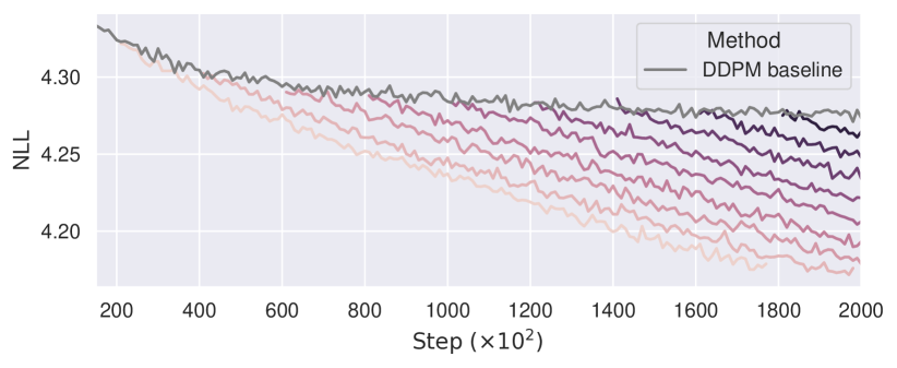
Figure 1: NLL performance of baseline and proposed methods. The gray line shows the results of the DDPM baseline; the colored lines show the results of the proposed GFlowNet consistency augmented training started with the pretrained weights of the baseline method from $20000,40000,\ldots,180000$ steps, respectively.

What’s more, we also try to finetune a pretrained model with our proposed method. Specifically, we train a DDPM model with a fixed number of steps, and then switch to the proposed MLE-GFN to continue the training. Figure 1 presents the curves of likelihood evaluation for the DDPM baseline (grey curve) and the proposed method (violet curves).

6 Conclusion

We have interpreted existing generative models as GFlowNets with different policies over sample trajectories. This provides some insight into the overlaps between existing generative modeling frameworks, and their connection to general-purpose algorithms for training them. Furthermore, this unification implies a method of constructing an agglomeration of varying types of generative modeling approaches, where GFlowNet acts as a general-purpose glue for tractable inference and training.

Appendix A Summary of Notation

Symbol	Description
$\mathcal{S}$	GFlowNet state space
$\mathcal{X}$	object (terminal state) space, subset of $\mathcal{S}$
$\mathcal{A}$	action / transition space (edges $\mathbf{s}\to\mathbf{s}^{\prime}$)
$\mathcal{G}$	directed acyclic graph $(\mathcal{S},\mathcal{A})$
$\mathcal{T}$	set of complete trajectories
$\mathbf{s}$	state in $\mathcal{S}$
$\mathbf{s}_{0}$	initial state, element of $\mathcal{S}$
$\mathbf{x}$	terminal state in $\mathcal{X}$
$\tau$	trajectory in $\mathcal{T}$
$F:\mathcal{T}\to\mathbb{R}$	Markovian flow
$F:\mathcal{S}\to\mathbb{R}$	state flow
$F:\mathcal{A}\to\mathbb{R}$	edge flow
$P_{F}(\mathbf{s}^{\prime}|\mathbf{s})$	forward policy (distribution over children)
$P_{B}(\mathbf{s}|\mathbf{s}^{\prime})$	backward policy (distribution over parents)
$P_{T}(\mathbf{x})$	terminating distribution
$Z$	scalar, equal to $\sum_{\tau\in\mathcal{T}}F(\tau)$ for a Markovian flow

Appendix B Proofs

B.1 Proposition 2

Proof.

We have

$$\mathcal{D}_{\mathrm{KL}}\left(P_{B}(\tau)\|P_{F}(\tau)\right) =\mathbb{E}_{p^{*}(\mathbf{x})q(\mathbf{z}_{1:n-1}|\mathbf{x})}\left[\log\frac{p^{*}(\mathbf{x})q(\mathbf{z}_{1:n-1}|\mathbf{x})}{p(\mathbf{z}_{1:n-1})p(\mathbf{x}|\mathbf{z}_{1:n-1})}\right]$$

$$=-\mathbb{E}_{p^{*}(\mathbf{x})}\mathbb{E}_{q(\mathbf{z}_{1:n-1}|\mathbf{x})}\left[\log\frac{p(\mathbf{x},\mathbf{z}_{1:n-1})}{q(\mathbf{z}_{1:n-1}|\mathbf{x})}\right]+\mathbb{E}_{p^{*}(\mathbf{x})}\left[\log p^{*}(\mathbf{x})\right]$$

$$=-\mathbb{E}_{p^{*}(\mathbf{x})}\left[\textrm{ELBO}_{p,q}(\mathbf{x})\right]-\mathcal{H}[p^{*}(\cdot)].$$

Here $\mathcal{H}[p^{*}(\cdot)]$ denotes the entropy of the target distribution, which is a constant w.r.t. GFlowNet parameters. ∎

B.2 Proposition 4

We follow a similar derivation of Ho et al. (2020) and Section B.1.

$$\mathcal{D}_{\mathrm{KL}}\left(P_{B}(\tau)\|P_{F}(\tau)\right) \cong-\mathbb{E}_{p^{*}(\mathbf{x})}\left[\textrm{ELBO}_{p,q}(\mathbf{x})\right]$$

$$\textrm{ELBO}_{p,q}(\mathbf{x}) =\mathbb{E}_{q}\left[-\log\frac{p(\mathbf{z}_{1:n})}{q(\mathbf{z}_{1:n-1}|\mathbf{x})}\right]=\mathbb{E}_{q}\left[-\log p(\mathbf{z}_{1})-\sum_{i<L}\log\frac{p(\mathbf{z}_{i+1}|\mathbf{z}_{i})}{q(\mathbf{z}_{i}|\mathbf{z}_{i+1})}-\log\frac{p(\mathbf{z}_{n}|\mathbf{z}_{L})}{q(\mathbf{z}_{L}|\mathbf{z}_{n})}\right]$$

$$=\mathbb{E}_{q}\left[-\log\frac{p(\mathbf{z}_{1})}{q(\mathbf{z}_{1}|\mathbf{z}_{n})}-\sum_{i<L}\log\frac{p(\mathbf{z}_{i+1}|\mathbf{z}_{i})}{q(\mathbf{z}_{i+1}|\mathbf{z}_{i},\mathbf{z}_{n})}-\log p(\mathbf{z}_{n}|\mathbf{z}_{L})\right]$$

$$\cong\mathbb{E}_{q}\left[\sum_{i<L}\mathcal{D}_{\mathrm{KL}}\left(q(\mathbf{z}_{i+1}|\mathbf{z}_{i},\mathbf{z}_{n})\|p(\mathbf{z}_{i+1}|\mathbf{z}_{i})\right)-\log p(\mathbf{z}_{n}|\mathbf{z}_{L})\right]$$

Since the KL divergence between two Gaussian distributions has a close form, we have

$$\mathcal{D}_{\mathrm{KL}}\left(q(\mathbf{z}_{i+1}|\mathbf{z}_{i},\mathbf{z}_{n})\|p(\mathbf{z}_{i+1}|\mathbf{z}_{i})\right) \cong C_{i}\cdot\mathbb{E}\left[\left\|\boldsymbol{\mu}_{i}(\mathbf{z}_{i})-\tilde{\boldsymbol{\mu}}_{i}(\mathbf{z}_{i})\right\|^{2}\right],$$

$$\mathbb{E}_{q}\left[-\log p(\mathbf{z}_{n}|\mathbf{z}_{L})\right] \cong C_{L}\cdot\mathbb{E}\left[\left\|\boldsymbol{\mu}_{L}(\mathbf{z}_{i})-\mathbf{z}_{n}\right\|^{2}\right],$$

where $\{C_{i}\}_{i}$ are scalar constants, and $\tilde{\boldsymbol{\mu}}_{i}(\mathbf{z}_{i})$ is the mean value of $q(\mathbf{z}_{i+1}|\mathbf{z}_{i},\mathbf{z}_{n})$, and $\tilde{\boldsymbol{\mu}}_{i}(\mathbf{z})=\tilde{C}_{i}^{1}\mathbf{z}+\tilde{C}_{i}^{2}\mathbf{x}$ is a fixed (i.e., non-learnable) transformation defined with $\{\beta_{i}\}_{i}$ and $\mathbf{x}=\mathbf{z}_{n}$. Here $\tilde{C}_{i}^{1},\tilde{C}_{i}^{2}$ are deterministic functions of $\{\beta_{i}\}_{i}$ defined by Ho et al. (2020). This derivation indicates that training a GFlowNet with KL-trajectory balance objective would end up with an effectively same (i.e., ignoring the constants) objective with the regression loss proposed in denoised autoencdoer (Vincent et al., 2008) and denoising diffusion probabilistic models.

B.3 Proposition 8

Proof.

First notice

$$\partial_{t}p(\mathbf{x},t)\triangleq\lim_{h\to 0}\frac{1}{h}\left(p(\mathbf{x},t+h)-p(\mathbf{x},t)\right)=\lim_{h\to 0}\frac{1}{h}\left(\int p(\mathbf{x}^{\prime},t)\mathbb{P}_{h}(\mathbf{x}|\mathbf{x}^{\prime})\mathop{}\!\mathrm{d}\mathbf{x}^{\prime}-p(\mathbf{x},t)\right).$$

Then for any function $w(\mathbf{x})$, we have

$$\quad\int w(\mathbf{x})\partial_{t}p(\mathbf{x},t)\mathop{}\!\mathrm{d}\mathbf{x}$$

$$=\int w(\mathbf{x})\lim_{h\to 0}\frac{1}{h}\left(\int p(\mathbf{x}^{\prime},t)\mathbb{P}_{h}(\mathbf{x}|\mathbf{x}^{\prime})\mathop{}\!\mathrm{d}\mathbf{x}^{\prime}-p(\mathbf{x},t)\right)\mathop{}\!\mathrm{d}\mathbf{x}$$

$$=\lim_{h\to 0}\frac{1}{h}\Large(\int w(\mathbf{x})\int p(\mathbf{x}^{\prime},t)\mathbb{P}_{h}(\mathbf{x}|\mathbf{x}^{\prime})\mathop{}\!\mathrm{d}\mathbf{x}^{\prime}\mathop{}\!\mathrm{d}\mathbf{x}-\int w(\mathbf{x}^{\prime})p(\mathbf{x}^{\prime},t)\int\mathbb{P}_{h}(\mathbf{x}|\mathbf{x}^{\prime})\mathop{}\!\mathrm{d}\mathbf{x}\mathop{}\!\mathrm{d}\mathbf{x}^{\prime}\Large)$$

$$=\lim_{h\to 0}\frac{1}{h}\int p(\mathbf{x}^{\prime},t)\mathbb{P}_{h}(\mathbf{x}|\mathbf{x}^{\prime})\left(w(\mathbf{x})-w(\mathbf{x}^{\prime})\right)\mathop{}\!\mathrm{d}\mathbf{x}\mathop{}\!\mathrm{d}\mathbf{x}^{\prime}$$

$$\triangleq\int p(\mathbf{x}^{\prime},t)\sum_{n=1}w^{(n)}(\mathbf{x}^{\prime})D_{n}(\mathbf{x}^{\prime})\mathbf{x}^{\prime}$$

$$=\int w(\mathbf{x}^{\prime})\sum_{n=1}\left(-\frac{\partial}{\partial\mathbf{x}^{\prime}}\right)^{n}\left(p(\mathbf{x}^{\prime},t)D_{n}(\mathbf{x}^{\prime})\right)\mathop{}\!\mathrm{d}\mathbf{x}^{\prime},$$

where $D_{n}(\mathbf{x}^{\prime})=\lim_{h\to 0}\frac{1}{hn!}\int\mathbb{P}_{h}(\mathbf{x}|\mathbf{x}^{\prime})(\mathbf{x}-\mathbf{x}^{\prime})^{n}\mathop{}\!\mathrm{d}\mathbf{x}$ and the last step uses integral by parts. This tells us

$$\partial_{t}p(\mathbf{x},t)=\sum_{n=1}\left(-\frac{\partial}{\partial\mathbf{x}}\right)^{n}\left(p(\mathbf{x},t)D_{n}(\mathbf{x})\right)=-\nabla_{\mathbf{x}}\left(p(\mathbf{x},t)\mathbf{f}(\mathbf{x},t)\right)+\frac{1}{2}\nabla_{\mathbf{x}}^{2}\left(p(\mathbf{x},t)g^{2}(\mathbf{x},t)\right),$$

which is essentially the Fokker-Planck equation.

∎

B.4 Proposition 9

From the above SDEs, we know that the forward and backward policy is

$$\mathbf{x}_{t+h} =\mathbf{x}_{t}+\mathbf{f}(\mathbf{x}_{t})h+\sqrt{h}g(t)\cdot{\boldsymbol{\delta}}_{F},$$

$$\mathbf{x}_{t} =\mathbf{x}_{t+h}+\left[g^{2}(t+h)\mathbf{s}(\mathbf{x}_{t+h})-\mathbf{f}(\mathbf{x}_{t+h})\right]h+\sqrt{h}g(t+h){\boldsymbol{\delta}}_{B},$$

where ${\boldsymbol{\delta}}_{F},{\boldsymbol{\delta}}_{B}\sim\mathcal{N}(0,\mathbf{I}_{D})$. Since we know $h\to 0$, the left and right side of  Equation 23 become

$$\log P_{F}(\mathbf{x}_{t+h}|\mathbf{x}_{t})-\log P_{B}(\mathbf{x}_{t}|\mathbf{x}_{t+h}) =-\frac{D}{2}\log(2\pi g^{2}_{t}h)-\frac{1}{2g_{t}^{2}h}\|\Delta\mathbf{x}-h\mathbf{f}_{t}\|^{2}$$

$$+\frac{D}{2}\log(2\pi g^{2}_{t+h}h)+\frac{1}{2g_{t+h}^{2}h}\|\Delta\mathbf{x}-h\mathbf{f}_{t+h}+hg^{2}_{t+h}\mathbf{s}(\mathbf{x}_{t+h})\|^{2},$$

$$\log p_{t+h}(\mathbf{x}_{t+h})-\log p_{t}(\mathbf{x}_{t}) =\Delta\mathbf{x}^{\top}\nabla_{\mathbf{x}}\log p_{t}(\mathbf{x})+O(h),$$

where $g_{t}=g(t),\mathbf{f}_{t}=\mathbf{f}(\mathbf{x}_{t}),\Delta\mathbf{x}=\mathbf{x}_{t+h}-\mathbf{x}_{t}=\sqrt{h}g_{t}{\boldsymbol{\epsilon}},{\boldsymbol{\epsilon}}\sim\mathcal{N}(0,\mathbf{I}_{D})$. Therefore,

$$\lim_{h\to 0}\frac{1}{\sqrt{h}g_{t}}(\log p_{t+h}(\mathbf{x}_{t+h})x-\log p_{t}(\mathbf{x}_{t}))={\boldsymbol{\epsilon}}^{\top}\nabla_{\mathbf{x}}\log p_{t}(\mathbf{x}),$$

$$\lim_{h\to 0}\frac{1}{\sqrt{h}g_{t}}(\log P_{F}(\mathbf{x}_{t+h}|\mathbf{x}_{t})-\log P_{B}(\mathbf{x}_{t}|\mathbf{x}_{t+h}))$$

$$=\lim_{h\to 0}\frac{D}{\sqrt{h}g_{t}}(\log g_{t+h}-\log g_{t})-\frac{1}{2g_{t}^{3}h^{3/2}}\left(hg_{t}^{2}\|{\boldsymbol{\epsilon}}\|^{2}+h^{2}\|\mathbf{f}_{t}\|^{2}-2h^{3/2}g_{t}{\boldsymbol{\epsilon}}^{\top}\mathbf{f}_{t}\right)$$

$$\phantom{aaaaaaaaaaaaa}+\frac{1}{2g_{t}g_{t+h}^{2}h^{3/2}}\left(hg_{t}^{2}\|{\boldsymbol{\epsilon}}\|^{2}-2h^{3/2}g_{t}{\boldsymbol{\epsilon}}^{\top}\mathbf{f}_{t+h}+2g_{t}g_{t+h}^{2}h^{3/2}{\boldsymbol{\epsilon}}^{\top}\mathbf{s}(\mathbf{x}_{t+h})\right)$$

$$=\lim_{h\to 0}{\boldsymbol{\epsilon}}^{\top}\left(\frac{\mathbf{f}_{t}}{g_{t}^{2}}-\frac{\mathbf{f}_{t+h}}{g_{t+h}^{2}}\right)+{\boldsymbol{\epsilon}}^{T}\mathbf{s}(\mathbf{x}_{t+h})={\boldsymbol{\epsilon}}^{T}\mathbf{s}(\mathbf{x}_{t}),$$

with some smoothness assumptions on $g(t)$ and $\mathbf{f}(\mathbf{x}_{t})/g(t)$. This tells us that in order to satisfy the detailed balance criterion, we need to satisfy

$${\boldsymbol{\epsilon}}^{\top}\left(\mathbf{s}(\mathbf{x}_{t},t)-\nabla_{\mathbf{x}}\log p_{t}(\mathbf{x})\right)=0,\forall{\boldsymbol{\epsilon}},\mathbf{x}_{t}\in\mathbb{R}^{D},\forall t\in[0,1].$$

Since ${\boldsymbol{\epsilon}}$ could take any value, this is equivalent that the model $\mathbf{s}$ should match with score function $\nabla_{\mathbf{x}}\log p(\mathbf{x})$. Also, note that this is exactly sliced score matching (Song et al., 2019), which has a more practical formulation

$$\mathbb{E}_{\boldsymbol{\epsilon}}\mathbb{E}_{\mathbf{x}\sim p}\left[{\boldsymbol{\epsilon}}^{\top}\nabla_{\mathbf{x}}\mathbf{s}(\mathbf{x}){\boldsymbol{\epsilon}}+\frac{1}{2}\left({\boldsymbol{\epsilon}}^{\top}\mathbf{s}(\mathbf{x})\right)^{2}\right].$$

B.5 Proposition 13

When both models (the GFlowNet and the discriminator) are trained perfectly, we have

$$D^{*}(\mathbf{x})=\frac{p^{*}(\mathbf{x})}{p^{*}(\mathbf{x})+p_{T}(\mathbf{x})},$$

and thus

$$p_{T}(\mathbf{x})\propto\exp\left(\log\frac{D^{*}(\mathbf{x})}{1-D^{*}(\mathbf{x})}+\log p_{T}(\mathbf{x})\right)=\exp\left(\log\frac{p^{*}(\mathbf{x})}{p_{T}(\mathbf{x})}+\log p_{T}(\mathbf{x})\right)=p^{*}(\mathbf{x}).$$

Hence it is a valid generative model algorithm.

B.6 Proposition 14

Because

$$\nabla_{{\boldsymbol{\phi}}}{\mathcal{L}_{\textrm{TBC}}}(\tau,\tau^{\prime})=2\left(\log\frac{P_{F}(\tau)}{P_{B}(\tau|\mathbf{x};{\boldsymbol{\phi}})}-\log\frac{P_{F}(\tau^{\prime})}{P_{B}(\tau^{\prime}|\mathbf{x};{\boldsymbol{\phi}})}\right)\left(-\nabla_{{\boldsymbol{\phi}}}\log P_{B}(\tau|\mathbf{x};{\boldsymbol{\phi}})+\nabla_{{\boldsymbol{\phi}}}\log P_{B}(\tau^{\prime}|\mathbf{x};{\boldsymbol{\phi}})\right),$$

we have

$$\frac{1}{2}\mathbb{E}_{\tau,\tau^{\prime}\sim P_{B}} \left[\nabla_{{\boldsymbol{\phi}}}{\mathcal{L}_{\textrm{TBC}}}(\tau,\tau^{\prime})\right]$$

$$= -\mathbb{E}_{\tau\sim P_{B}}\left[\log\frac{P_{F}(\tau)}{P_{B}(\tau|\mathbf{x};{\boldsymbol{\phi}})}\nabla_{{\boldsymbol{\phi}}}\log P_{B}(\tau|\mathbf{x};{\boldsymbol{\phi}})\right]+\mathbb{E}_{\tau,\tau^{\prime}\sim P_{B}}\left[\log\frac{P_{F}(\tau)}{P_{B}(\tau|\mathbf{x};{\boldsymbol{\phi}})}\nabla_{{\boldsymbol{\phi}}}\log P_{B}(\tau^{\prime}|\mathbf{x};{\boldsymbol{\phi}})\right]$$

$$-\mathbb{E}_{\tau^{\prime}\sim P_{B}}\left[\log\frac{P_{F}(\tau^{\prime})}{P_{B}(\tau^{\prime}|\mathbf{x};{\boldsymbol{\phi}})}\nabla_{{\boldsymbol{\phi}}}\log P_{B}(\tau^{\prime}|\mathbf{x};{\boldsymbol{\phi}})\right]+\mathbb{E}_{\tau,\tau^{\prime}\sim P_{B}}\left[\log\frac{P_{F}(\tau^{\prime})}{P_{B}(\tau^{\prime}|\mathbf{x};{\boldsymbol{\phi}})}\nabla_{{\boldsymbol{\phi}}}\log P_{B}(\tau|\mathbf{x};{\boldsymbol{\phi}})\right]$$

$$= -2\mathbb{E}_{\tau\sim P_{B}}\left[\log\frac{P_{F}(\tau)}{P_{B}(\tau|\mathbf{x};{\boldsymbol{\phi}})}\nabla_{{\boldsymbol{\phi}}}\log P_{B}(\tau|\mathbf{x};{\boldsymbol{\phi}})\right]+\mathbb{E}_{\tau\sim P_{B}}\left[\log\frac{P_{F}(\tau)}{P_{B}(\tau|\mathbf{x};{\boldsymbol{\phi}})}\right]\underbrace{\mathbb{E}_{\tau^{\prime}\sim P_{B}}\left[\nabla_{{\boldsymbol{\phi}}}\log P_{B}(\tau^{\prime}|\mathbf{x};{\boldsymbol{\phi}})\right]}_{=0}$$

$$= 2\nabla_{{\boldsymbol{\phi}}}\mathbb{E}_{\tau\sim P_{B}}\left[\log\frac{P_{B}(\tau|\mathbf{x};{\boldsymbol{\phi}})}{P_{F}(\tau)}\right]$$

$$= 2\nabla_{{\boldsymbol{\phi}}}\mathcal{D}_{\mathrm{KL}}\left(P_{B}\|P_{F}\right)$$

Appendix C More about Experimental Demonstration

C.1 Synthetic Demonstration

2spirals

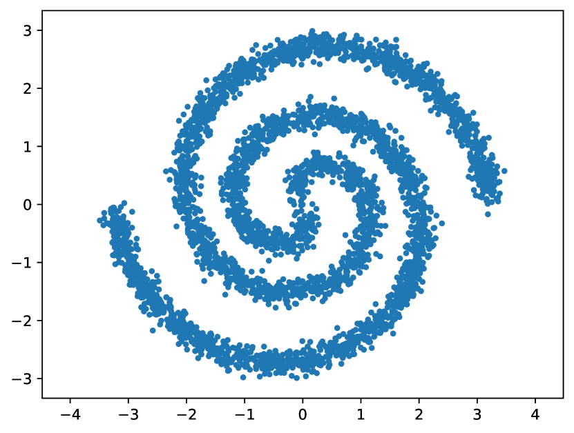
8gaussians

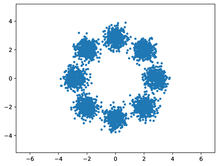
circles

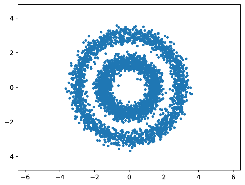
moons

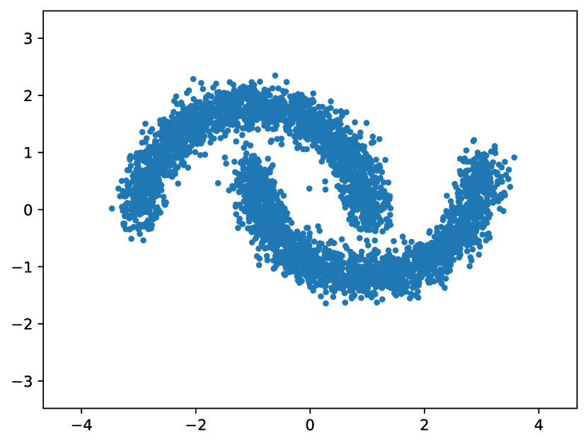
pinwheel

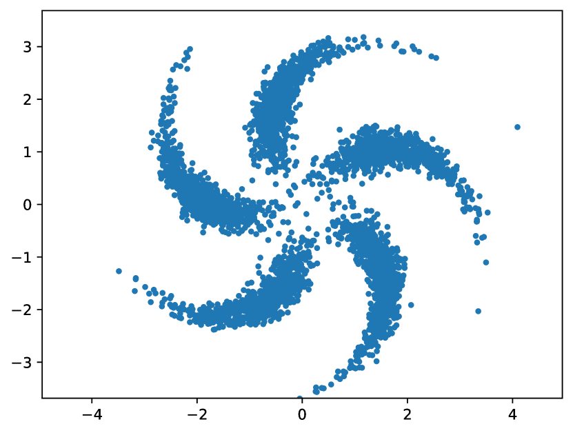
swissroll

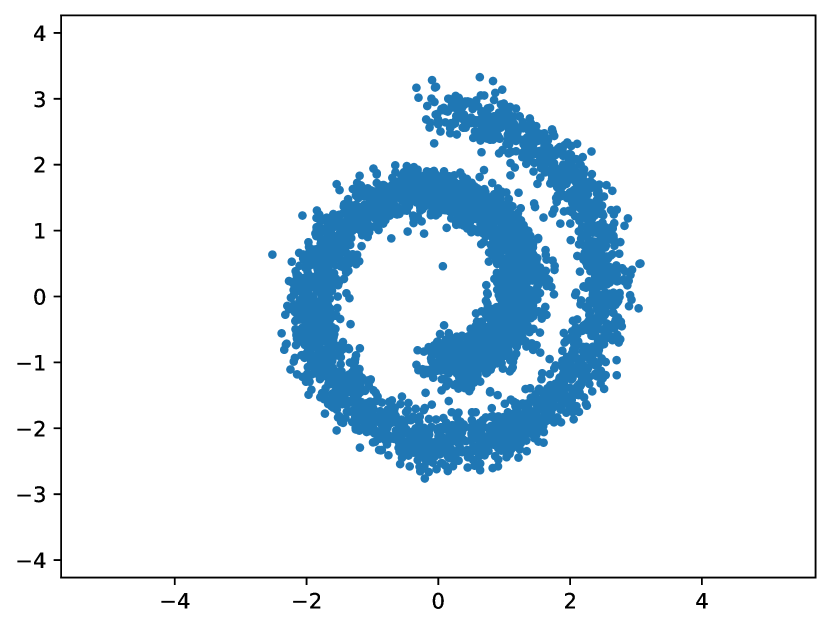
checkerboard

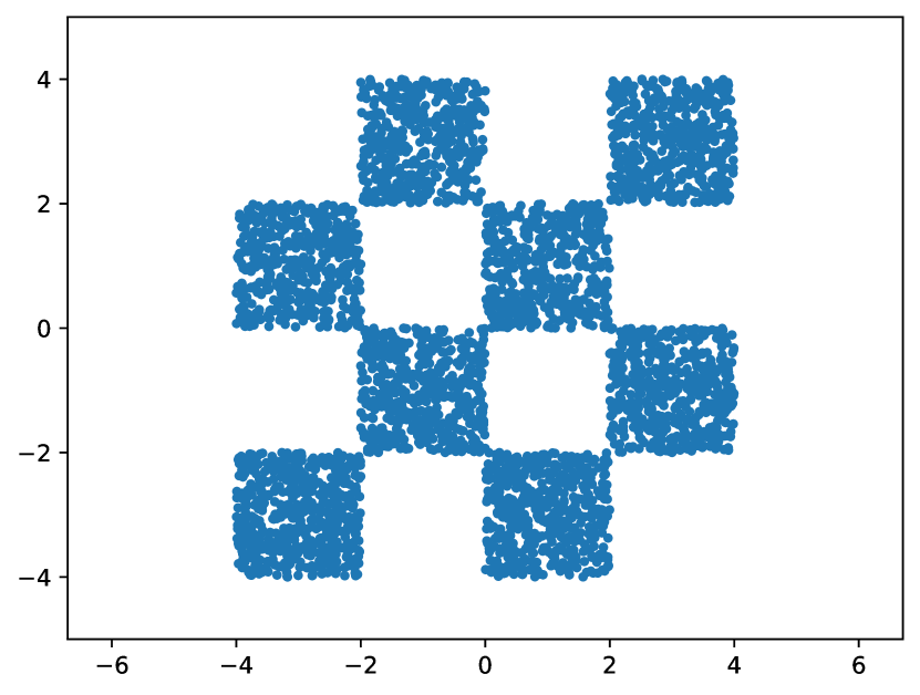
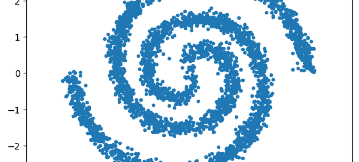
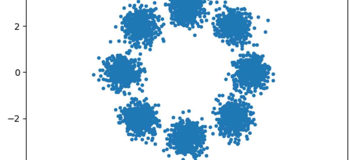
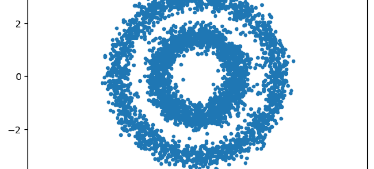
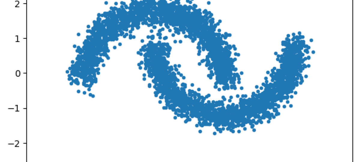
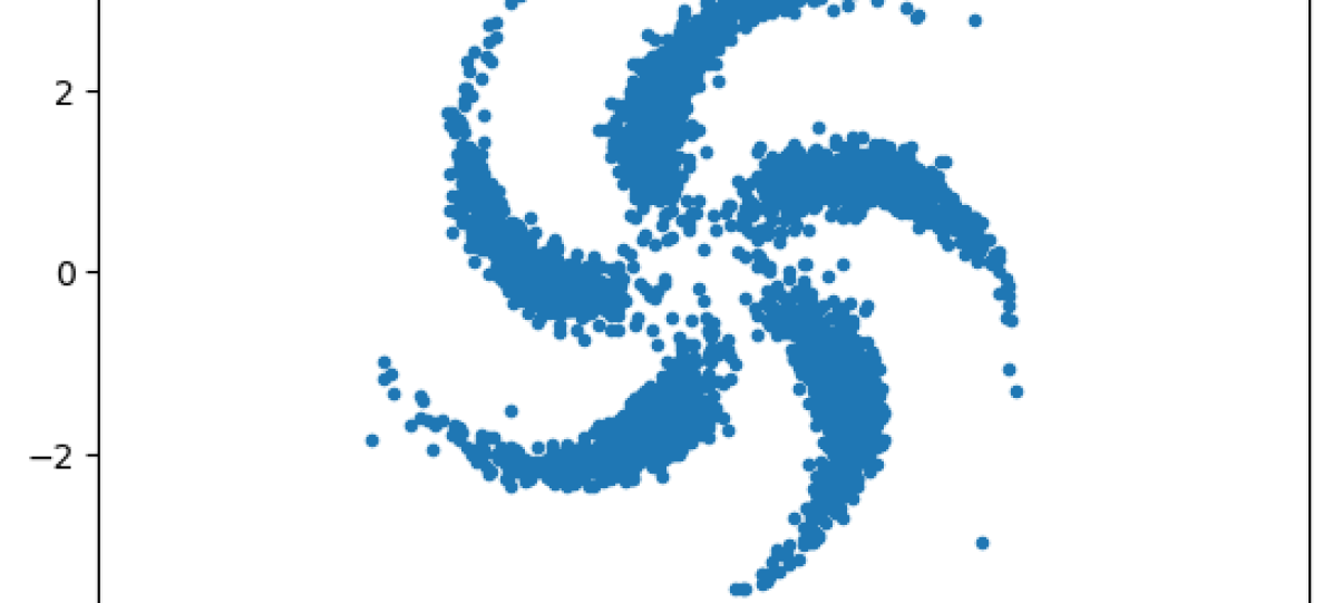
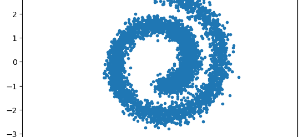
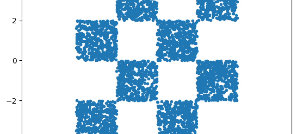
Figure 2: Top: Visualization of the samples for synthetic problems from ground truth. Bottom: Visualization of the samples generated with the proposed GFlowNet-based algorithm.

Table 3: Experiment results with seven 2D synthetic problems. We display the negative loglikelihood (NLL).

Metric	Method	2spirals	8gaussians	circles	moons	pinwheel	swissroll	checkerboard
NLL$\downarrow$	PCD	$20.094$	$19.991$	$20.565$	$19.763$	$19.593$	$20.172$	$21.214$
	ALOE	$20.295$	$20.350$	$20.565$	$19.287$	$19.821$	$20.160$	$54.653$
	ALOE+	$20.062$	$19.984$	$20.570$	$19.743$	$19.576$	$20.170$	$21.142$
	EB-GFN	20.050	${19.982}$	20.546	${19.732}$	19.554	20.146	${20.696}$
	TBC-GFN	20.050	19.965	${20.554}$	19.719	19.555	20.144	20.682

We visualize the ground truth samples and GFlowNet generated samples in its $2$-D form in Figure 2. We also demonstrate the likelihood evaluation results in Table 3, which indicates that the proposed method achieves a fairly good level of distribution fitting. Regarding training details, we use the Adam optimizer with $1\times 10^{-4}$ and $1\times 10^{-5}$ for learning the forward and backward policy, respectively. The training keeps $100000$ steps. The evaluation of exponential MMD is calculated through average over $10$ sets of samples, each set contain $4000$ samples, which is the same as with Zhang et al. (2022b). All other setup follows Zhang et al. (2022b), too.

C.2 DDPM Demonstration

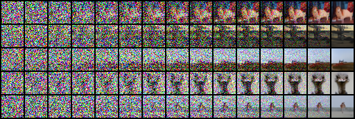
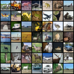
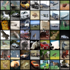
Figure 3: Left: visualization of trajectory examples on CIFAR-$10$ image space. Right: MLE-GFN generated samples.

We train on a single V100 GPU for $200$k steps, which takes less than three days. We use the Adam optimizer with a learning rate of $2\times 10^{-4}$ for updating the forward policy and a learning rate of $2\times 10^{-5}$ for updating the backward policy. All NLL results are computed in the unit of bits per dim (BPD). The denoising process (forward policy) is parameterized with a UNet as done by Ho et al. (2020). The backward policy is parameterized in the way that its parameter ${\boldsymbol{\phi}}=\{\phi_{i}\}_{i},\beta_{i}=\bar{\beta}_{i}\cdot\exp{(\phi_{i})}$, where $\{\bar{\beta}_{i}\}_{i}$ are the original variance parameters from Ho et al. (2020). We also visualize several trajectories of the GFlowNet in Figure 3 (left), where the intermediate state is updated with the forward policy from the left-hand side to the right-hand side of the figure. In Figure 3 (right), we visualize several generated image samples from MLE-GFN training on CIFAR-$10$ dataset.

References

- Agarwal et al. (2020) Agarwal, R., Schuurmans, D., and Norouzi, M. An optimistic perspective on offline reinforcement learning. International Conference on Machine Learning (ICML), 2020.
- Anderson (1982) Anderson, B. D. O. Reverse-time diffusion equation models. Stochastic Processes and their Applications, 12:313–326, 1982.
- Austin et al. (2021) Austin, J., Johnson, D. D., Ho, J., Tarlow, D., and van den Berg, R. Structured denoising diffusion models in discrete state-spaces. Neural Information Processing Systems (NeurIPS), 2021.
- Bengio et al. (2021a) Bengio, E., Jain, M., Korablyov, M., Precup, D., and Bengio, Y. Flow network based generative models for non-iterative diverse candidate generation. Neural Information Processing Systems (NeurIPS), 2021a.
- Bengio & Bengio (1999) Bengio, Y. and Bengio, S. Modeling high-dimensional discrete data with multi-layer neural networks. Neural Information Processing Systems (NIPS), 1999.
- Bengio et al. (2021b) Bengio, Y., Deleu, T., Hu, E. J., Lahlou, S., Tiwari, M., and Bengio, E. GFlowNet foundations. arXiv preprint 2111.09266, 2021b.
- Blei et al. (2001) Blei, D. M., Ng, A., and Jordan, M. I. Latent dirichlet allocation. J. Mach. Learn. Res., 3:993–1022, 2001.
- Bortoli et al. (2021) Bortoli, V. D., Thornton, J., Heng, J., and Doucet, A. Diffusion schrödinger bridge with applications to score-based generative modeling. Neural Information Processing Systems (NeurIPS), 2021.
- Burda et al. (2016) Burda, Y., Grosse, R. B., and Salakhutdinov, R. Importance weighted autoencoders. arXiv preprint 1509.00519, 2016.
- Che et al. (2020) Che, T., Zhang, R., Sohl-Dickstein, J., Larochelle, H., Paull, L., Cao, Y., and Bengio, Y. Your gan is secretly an energy-based model and you should use discriminator driven latent sampling. Neural Information Processing Systems (NeurIPS), 2020.
- Chen et al. (2021) Chen, Y., Georgiou, T. T., and Pavon, M. Optimal transport in systems and control. Annual Review of Control, Robotics, and Autonomous Systems, 4(1), 2021.
- Child (2021) Child, R. Very deep VAEs generalize autoregressive models and can outperform them on images. International Conference on Learning Representations (ICLR), 2021.
- Dai et al. (2020) Dai, H., Singh, R., Dai, B., Sutton, C., and Schuurmans, D. Learning discrete energy-based models via auxiliary-variable local exploration. arXiv preprint 2011.05363, 2020.
- Dayan et al. (1995) Dayan, P., Hinton, G. E., Neal, R. M., and Zemel, R. S. The helmholtz machine. Neural Computation, 7:889–904, 1995.
- Deleu et al. (2022) Deleu, T., G’ois, A., Emezue, C. C., Rankawat, M., Lacoste-Julien, S., Bauer, S., and Bengio, Y. Bayesian structure learning with generative flow networks. Uncertainty in Artificial Intelligence (UAI), 2022.
- Dhariwal & Nichol (2021) Dhariwal, P. and Nichol, A. Diffusion models beat GANs on image synthesis. Neural Information Processing Systems (NeurIPS), 2021.
- Dinh et al. (2014) Dinh, L., Krueger, D., and Bengio, Y. NICE: Non-linear independent components estimation. arXiv preprint 1410.8516, 2014.
- Dinh et al. (2015) Dinh, L., Krueger, D., and Bengio, Y. Nice: Non-linear independent components estimation. arXiv preprint 1410.8516, 2015.
- Goodfellow et al. (2014) Goodfellow, I. J., Pouget-Abadie, J., Mirza, M., Xu, B., Warde-Farley, D., Ozair, S., Courville, A. C., and Bengio, Y. Generative adversarial nets. Neural Information Processing Systems (NIPS), 2014.
- Goyal & Bengio (2020) Goyal, A. and Bengio, Y. Inductive biases for deep learning of higher-level cognition. Proceedings of the Royal Society A, 478, 2020.
- Gray (1953) Gray, F. Pulse code communication. United States Patent Number 2632058, 1953.
- Gretton et al. (2012) Gretton, A., Borgwardt, K. M., Rasch, M. J., Schölkopf, B., and Smola, A. A kernel two-sample test. J. Mach. Learn. Res., 13:723–773, 2012.
- Gu et al. (2018) Gu, J., Bradbury, J., Xiong, C., Li, V. O. K., and Socher, R. Non-autoregressive neural machine translation. International Conference on Learning Representations (ICLR), 2018.
- Henderson et al. (2017) Henderson, P., Islam, R., Bachman, P., Pineau, J., Precup, D., and Meger, D. Deep reinforcement learning that matters. Association for the Advancement of Artificial Intelligence (AAAI), 2017.
- Heusel et al. (2017) Heusel, M., Ramsauer, H., Unterthiner, T., Nessler, B., and Hochreiter, S. GANs trained by a two time-scale update rule converge to a local nash equilibrium. Neural Information Processing Systems (NIPS), 2017.
- Hinton (2002) Hinton, G. E. Training products of experts by minimizing contrastive divergence. Neural Computation, 14:1771–1800, 2002.
- Hinton et al. (1995) Hinton, G. E., Dayan, P., Frey, B. J., and Neal, R. M. The "wake-sleep" algorithm for unsupervised neural networks. Science, 268 5214:1158–61, 1995.
- Ho et al. (2020) Ho, J., Jain, A., and Abbeel, P. Denoising diffusion probabilistic models. Neural Information Processing Systems (NeurIPS), 2020.
- Hoogeboom et al. (2021) Hoogeboom, E., Nielsen, D., Jaini, P., Forr’e, P., and Welling, M. Argmax flows and multinomial diffusion: Learning categorical distributions. Neural Information Processing Systems (NeurIPS), 2021.
- Hu et al. (2018) Hu, Z., Yang, Z., Salakhutdinov, R., and Xing, E. P. On unifying deep generative models. International Conference on Learning Representations (ICLR), 2018.
- Huang et al. (2021) Huang, C.-W., Lim, J. H., and Courville, A. C. A variational perspective on diffusion-based generative models and score matching. Neural Information Processing Systems (NeurIPS), 2021.
- Jain et al. (2022a) Jain, M., Bengio, E., García, A., Rector-Brooks, J., Dossou, B. F. P., Ekbote, C. A., Fu, J., Zhang, T., Kilgour, M., Zhang, D., Simine, L., Das, P., and Bengio, Y. Biological sequence design with GFlowNets. International Conference on Machine Learning (ICML), 2022a.
- Jain et al. (2022b) Jain, M., Raparthy, S. C., Hernández-García, A., Rector-Brooks, J., Bengio, Y., Miret, S., and Bengio, E. Multi-objective gflownets. arXiv preprint 2210.12765, 2022b.
- Kingma & Welling (2013) Kingma, D. P. and Welling, M. Auto-encoding variational Bayes. arXiv preprint 1312.6114, 2013.
- Kingma et al. (2021) Kingma, D. P., Salimans, T., Poole, B., and Ho, J. Variational diffusion models. Neural Information Processing Systems (NeurIPS), 2021.
- Koller & Friedman (2009) Koller, D. and Friedman, N. Probabilistic graphical models: principles and techniques. MIT press, 2009.
- Kullback (1968) Kullback, S. Probability densities with given marginals. Annals of Mathematical Statistics, 39:1236–1243, 1968.
- Lahlou et al. (2023) Lahlou, S., Deleu, T., Lemos, P., Zhang, D., Volokhova, A., Hernández-García, A., Ezzine, L. N., Bengio, Y., and Malkin, N. A theory of continuous generative flow networks. arXiv preprint 2301.12594, 2023.
- Lange et al. (2012) Lange, S., Gabel, T., and Riedmiller, M. A. Batch reinforcement learning. In Reinforcement Learning, 2012.
- LeCun et al. (2006) LeCun, Y., Chopra, S., Hadsell, R., Ranzato, A., and Huang, F. J. A tutorial on energy-based learning. In Predicting Structured Data. MIT Press, 2006.
- Léonard (2013) Léonard, C. A survey of the Schrödinger problem and some of its connections with optimal transport. arXiv preprint 1308.0215, 2013.
- Lin (2004) Lin, L. Self-improving reactive agents based on reinforcement learning, planning and teaching. Machine Learning, 8:293–321, 2004.
- Liu et al. (2022) Liu, D., Jain, M., Dossou, B. F. P., Shen, Q., Lahlou, S., Goyal, A., Malkin, N., Emezue, C. C., Zhang, D., Hassen, N., Ji, X., Kawaguchi, K., and Bengio, Y. GFlowOut: Dropout with generative flow networks. arXiv preprint 2210.12928, 2022.
- Madan et al. (2022) Madan, K., Rector-Brooks, J., Korablyov, M., Bengio, E., Jain, M., Nica, A. C., Bosc, T., Bengio, Y., and Malkin, N. Learning gflownets from partial episodes for improved convergence and stability. arXiv preprint 2209.12782, 2022.
- Malkin et al. (2022) Malkin, N., Jain, M., Bengio, E., Sun, C., and Bengio, Y. Trajectory balance: Improved credit assignment in GFlowNets. arXiv preprint 2201.13259, 2022.
- Malkin et al. (2023) Malkin, N., Lahlou, S., Deleu, T., Ji, X., Hu, E., Everett, K., Zhang, D., and Bengio, Y. GFlowNets and variational inference. International Conference on Learning Representations (ICLR), 2023. To appear.
- Murphy (2012) Murphy, K. P. Machine learning: a probabilistic perspective. 2012.
- Nichol & Dhariwal (2021) Nichol, A. and Dhariwal, P. Improved denoising diffusion probabilistic models. International Conference on Machine Learning (ICML), 2021.
- Øksendal (1985) Øksendal, B. Stochastic differential equations. The Mathematical Gazette, 77:65–84, 1985.
- Pan et al. (2022) Pan, L., Zhang, D., Courville, A. C., Huang, L., and Bengio, Y. Generative augmented flow networks. arXiv preprint 2210.03308, 2022.
- Ranganath et al. (2016) Ranganath, R., Tran, D., and Blei, D. M. Hierarchical variational models. International Conference on Machine Learning (ICML), 2016.
- Schrödinger (1932) Schrödinger, E. Sur la théorie relativiste de l’électron et l’interprétation de la mécanique quantique. Annales de l’institut Henri Poincaré, 2(4):269–310, 1932.
- Shi et al. (2022) Shi, Y., Bortoli, V. D., Deligiannidis, G., and Doucet, A. Conditional simulation using diffusion schrödinger bridges. Uncertainty in Artificial Intelligence (UAI), 2022.
- Shu & Ermon (2022) Shu, R. and Ermon, S. Bit prioritization in variational autoencoders via progressive coding. International Conference on Machine Learning (ICML), 2022.
- Sohl-Dickstein et al. (2015) Sohl-Dickstein, J. N., Weiss, E. A., Maheswaranathan, N., and Ganguli, S. Deep unsupervised learning using nonequilibrium thermodynamics. International Conference on Machine Learning (ICML), 2015.
- Sønderby et al. (2016) Sønderby, C. K., Raiko, T., Maaløe, L., Sønderby, S. K., and Winther, O. Ladder variational autoencoders. Neural Information Processing Systems (NIPS), 2016.
- Song et al. (2019) Song, Y., Garg, S., Shi, J., and Ermon, S. Sliced score matching: A scalable approach to density and score estimation. Uncertainty in Artificial Intelligence (UAI), 2019.
- Song et al. (2020) Song, Y., Sohl-Dickstein, J. N., Kingma, D. P., Kumar, A., Ermon, S., and Poole, B. Score-based generative modeling through stochastic differential equations. International Conference on Learning Representations (ICLR), 2020.
- Song et al. (2021) Song, Y., Durkan, C., Murray, I., and Ermon, S. Maximum likelihood training of score-based diffusion models. Neural Information Processing Systems (NeurIPS), 2021.
- Sutton & Barto (2005) Sutton, R. S. and Barto, A. G. Reinforcement learning: An introduction. IEEE Transactions on Neural Networks, 16:285–286, 2005.
- Tieleman (2008) Tieleman, T. Training restricted Boltzmann machines using approximations to the likelihood gradient. International Conference on Machine Learning (ICML), 2008.
- Tzen & Raginsky (2019) Tzen, B. and Raginsky, M. Neural stochastic differential equations: Deep latent gaussian models in the diffusion limit. arXiv preprint 1905.09883, 2019.
- van den Oord et al. (2016) van den Oord, A., Kalchbrenner, N., and Kavukcuoglu, K. Pixel recurrent neural networks. International Conference on Machine Learning (ICML), 2016.
- Vincent (2011) Vincent, P. A connection between score matching and denoising autoencoders. Neural Computation, 23:1661–1674, 2011.
- Vincent et al. (2008) Vincent, P., Larochelle, H., Bengio, Y., and Manzagol, P.-A. Extracting and composing robust features with denoising autoencoders. International Conference on Machine Learning (ICML), 2008.
- Zhang et al. (2021) Zhang, D., Fu, J., Bengio, Y., and Courville, A. C. Unifying likelihood-free inference with black-box optimization and beyond. International Conference on Learning Representations (ICLR), 2021.
- Zhang et al. (2022a) Zhang, D., Courville, A. C., Bengio, Y., Zheng, Q., Zhang, A., and Chen, R. T. Q. Latent state marginalization as a low-cost approach for improving exploration. arXiv preprint 2210.00999, 2022a.
- Zhang et al. (2022b) Zhang, D., Malkin, N., Liu, Z., Volokhova, A., Courville, A. C., and Bengio, Y. Generative flow networks for discrete probabilistic modeling. International Conference on Machine Learning (ICML), 2022b.