Resonant leptoquark at NLO with POWHEG
Abstract
Recent progress in calculating lepton density functions inside the proton and simulating lepton showers laid the foundations for precision studies of resonant leptoquark production at hadron colliders. Direct quark-lepton fusion into a leptoquark is a novel production channel at the LHC that has the potential to probe a unique parameter space for large masses and couplings. In this work, we build the first Monte Carlo event generator for a full-fledged simulation of this process at NLO for production, followed by a subsequent decay using the POWHEG method and matching to the parton showers utilizing HERWIG. The code can handle all scalar leptoquark models with renormalisable quark-lepton interactions. We then comprehensively study the differential distributions, including higher-order effects, and asses the corresponding theoretical uncertainties. We also quantify the impact of the improved predictions on the projected (HL-)LHC sensitivities and initiate the first exploration of the potential at the FCC-hh. Our work paves the way toward performing LHC searches using this channel.
Keywords:
Perturbative QCD, NLO computations, Leptoquark1 Introduction
Leptoquarks are hypothetical spin- or spin- particles carrying both lepton and baryon numbers and mediating a novel interaction among quarks and leptons. They stem from various theories beyond the Standard Model (SM), motivated by the idea of quark-lepton unification. They are predicted in scenarios of matter unification à la Pati-Salam Pati:1974yy involving gauge group or in grand unification theories with larger gauge groups like Georgi:1974sy , and Fritzsch:1974nn . The phenomenology of leptoquarks is a mature topic (for a recent review see Dorsner:2016wpm ), relevant for both low- and high-energy experiments. Leptoquarks at the TeV scale are particularly interesting for high-energy colliders.
The mass range accessible at colliders is motivated by several extensions of the SM. Scalar leptoquarks arise as pseudo-Nambu-Goldstone bosons of a new strongly interacting sector possibly stabilising the electroweak scale and solving the Higgs hierarchy problem Gripaios:2009dq ; Fuentes-Martin:2020bnh ; Barbieri:2017tuq ; Sannino:2017utc ; Marzocca:2018wcf , and are also present in R-parity violating supersymmetric settings Giudice:1997wb ; Csaki:2011ge ; Altmannshofer:2020axr ; Dreiner:2021ext . Vector leptoquarks at the TeV scale are predicted in the partial unification models based on the gauge group DiLuzio:2017vat ; Bordone:2017bld ; Greljo:2018tuh ; Fornal:2018dqn ; Heeck:2018ntp ; Cornella:2019hct ; Blanke:2018sro ; Balaji:2019kwe . Indirectly, the presence of leptoquarks would impact the low-energy flavour transitions, electroweak precision observables, and Higgs physics. At hadron colliders, a leptoquark would be identifiable as a resonance in the invariant mass of a lepton plus a jet system.
The renewed interest in TeV-scale leptoquarks in recent years originates from several experimental anomalies in semileptonic decays of -mesons Lees:2013uzd ; Hirose:2016wfn ; Aaij:2015yra ; Aaij:2014ora ; Aaij:2017vbb ; Aaij:2013qta ; Aaij:2015oid ; Aaij:2019wad which naturally highlight leptoquarks as possible explanation candidates. This is because leptoquarks contribute to the semileptonic transitions at the tree level. At the same time, they affect dangerous four-quark or four-lepton flavour-changing neutral currents, well described by the SM, at the one-loop level only. With anomalies continuing to persist, the TeV-scale leptoquarks with couplings to the SM fermions are a clear target for current and future collider searches. Motivated in part by the developments in flavour physics, there has been an increasing effort within ATLAS and CMS experiments to hunt for leptoquarks (for recent results see ATLAS:2021jyv ; ATLAS:2021oiz ; ATLAS:2019qpq ; ATLAS:2020xov ; ATLAS:2020dsk ; CMS:2020wzx ; CMS:2018oaj ; CMS:2018qqq ; CMS:2022nty ; CMS:2021far ).
Since leptoquarks couple quarks and leptons, they necessarily carry charge and can thus be pair produced in gluon fusion Blumlein:1996qp ; Kramer:1997hh ; Kramer:2004df ; Diaz:2017lit ; Borschensky:2020hot ; Allanach:2019zfr ; Borschensky:2022xsa ; Dorsner:2018ynv . This production mechanism is dominant for small values of the leptoquark to quark and lepton coupling , depending only on the leptoquark mass and the strong coupling . However, the pair production is not optimal for heavy leptoquark searches due to rapid phase-space suppression with increasing leptoquark mass. For this reason, often discussed in the literature is the single leptoquark plus lepton production from quark-gluon scattering Alves:2002tj ; Hammett:2015sea ; Mandal:2015vfa ; Dorsner:2018ynv . The production cross section for this process is proportional to , but suffers less phase-space suppression, and for coupling, it compares to, and even wins over, the cross section for leptoquark pair production. Finally, a non-resonant effect of leptoquarks in the -channel Drell-Yan process could be seen as a deviation in the high- tail of the dilepton invariant mass distribution Faroughy:2016osc ; Greljo:2017vvb ; Schmaltz:2018nls ; Fuentes-Martin:2020lea ; Greljo:2018tzh ; Marzocca:2020ueu ; Baker:2019sli ; Allwicher:2022gkm . Since, in this case, the cross-section scales as , the expectation is that this process dominates the leptoquark signatures for large couplings and masses beyond the kinematical reach for on-shell production.
Resonant leptoquark production from a direct lepton-quark fusion is another relevant process at a hadron collider put forward in Ohnemus:1994xf . However, before the precise determination of leptonic parton distribution functions (PDF) inside the proton in Buonocore:2020nai , this process could not be utilized in practice. The work of Buonocore:2020nai , therefore, provides a novel opportunity to discover leptoquarks at the LHC. The production cross section scales as and enjoys the least phase-space suppression, making it the most sensitive process for certain parameter regions with couplings and TeV-scale masses. The phenomenological collider simulation for this channel, performed in Buonocore:2020erb ; Haisch:2020xjd , confirmed this statement and established the resonant leptoquark production mechanism as an exciting candidate for future experimental analyses. In particular, this mechanism surpasses the single leptoquark plus lepton production, which also scales as .
However, the limitation of Buonocore:2020erb ; Haisch:2020xjd is the inadequate signal modeling, more precisely, the tree-level approximation and the absence of a lepton shower not available at the time. In this context, the recent computation of next-to-leading (NLO) corrections in Greljo:2020tgv , and the development of a lepton shower in Bewick:2021nhc , constitute a first step toward exploiting the full potential of the resonant leptoquark production, allowing for more advanced precision studies.
In this paper, we make a significant leap forward by constructing a full-fledged Monte Carlo tool for the resonant leptoquark production from a lepton-quark fusion at NLO merged with QCD and lepton showers. By NLO, we mean here that we include QCD corrections and a subset of enhanced QED corrections that makes them comparable with the QCD ones, as we will explain in due time. We quantify the impact of higher-order corrections on the differential phase-space distributions. We assess the importance of the improved signal modeling on the projected LHC bounds derived in Buonocore:2020erb . Additionally, we compute the inclusive cross sections for 100 TeV proton-proton center-of-mass energy and briefly discuss the potential offered by a future circular hadron collider (FCC-hh) FCC:2018vvp . Our ready-to-use Monte Carlo event generator will facilitate further phenomenological studies and enable the first experimental searches for this process at the LHC.
The paper is organised as follows. In Section 2, we describe the implementation of the resonant leptoquark production in the Powheg framework. In Section 2.1, we define the scope of the leptoquark models and present the expressions for the required amplitudes at NLO. In Section 2.2, we discuss the treatment of the total decay width, while in Section 2.3 we report on the modifications of the Powheg-Box needed to support this process. In Section 3, we discuss the most important phenomenological imprints of the resonant leptoquark production mechanism. In Section 3.1, we validate the implementation against the inclusive NLO cross sections reported in Greljo:2020tgv and provide new results for 100 TeV collider. In Section 3.2, with quantify the impact of NLO corrections and parton shower effects on the differential distributions. In Section 3.3, we quantify the error made due to the limited signal simulation in the sensitivity study of Buonocore:2020erb . In Section 3.4, we showcase a model example, the leptoquark. In particular, we estimate the sensitivity reach of 100 TeV proton-proton collider in the mass versus coupling plane. We finally conclude in Section 4.
2 Implementation within the Powheg-Box
In this section we develop a Monte Carlo tool for the resonant leptoquark production at NLO (and subsequent decay) capable of generating Les Houches events (LHE) that can be directly processed by a Parton Shower (PS) program in order to obtain a complete simulation of the collision at the NLO+PS level.
2.1 Leptoquark models and scattering amplitudes
Our goal is a Powheg-Box-Res implementation of the resonant leptoquark production at NLO in both QCD and QED for all renormalisable scalar leptoquark models. The starting point is the Lagrangian in the broken phase, i.e. respecting gauge symmetry,
| (1) |
where are general Yukawa coupling matrices in flavour space, and are the chiral projectors. The SM chiral fermions and correspond to the mass eigenstates after the electroweak symmetry breaking. In general terms, the scalar leptoquarks, , are triplets of , with their possible charges being . The viable flavour structure of the Born process involves the quark flavours (and at FCC-hh) and charged leptons . For instance, a -quark and a -lepton can be used to create and leptoquarks, as specified by . Note that any renormalisable scalar leptoquark model defined respecting the full SM gauge symmetry Dorsner:2016wpm can be recast in the form of Eq. (1) by separately considering the different components of the leptoquark representation. In Section 3.4, we will exemplify this with a weak triplet.
Next, we present the expressions for the amplitudes that are used by the code. Starting with the leading order (Born level), the resonant leptoquark production proceeds via fusion of a lepton and a quark in the initial state. Given the energies of the colliders in consideration, we approximate the aforementioned fermions to be massless, such that the possible interference terms between left- and right-handed Yukawa couplings vanish. Thus, the averaged squared matrix element for a particular flavour combination at the Born level reads
| born | (2) |
where is the partonic-level center of mass energy. Moreover, when different flavour combinations in the initial state contribute to the production of the same leptoquark, the contributions to the averaged squared matrix element are added separately. The expression born matches the input of the Powheg-Box-Res that the process-specific code should provide in the routine
setborn(p(0:3,1:nlegborn), bflav(1:nlegborn), born,
bornjk(1:nlegborn,1:nlegborn), bmunu(0:3,0:3,1:nlegborn)) .
In our case, since we are dealing with the process, we set , and p(0:3,i) denote the components of the four-momenta of the i-th particle. We enumerate the particles in the process as , respectively, such that , while the color correlated squared amplitude, bornjk, and the spin correlated one, bmunu, read
| bornjk(1,2) | (3) | |||
| bornjk(1,3) | (4) | |||
| bmunu | (5) |
as explained in Alioli:2010xd , with bornjk being symmetric.
Apart from the leading (Born) contribution, this process receives important NLO corrections from interactions with gluons and photons. As shown in Greljo:2020tgv , the QED corrections that we need to include are such that the smallness of the QED coupling is compensated by the PDF enhancement due to the photon in the initial state of the process , so that they are in fact of the same order as the QCD corrections.
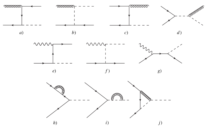
In the context of QCD corrections, the first relevant partonic process is , shown in Figure 1 and . The partonic cross-section for this process was computed in Kunszt:1997at ; Plehn:1997az .111Notice that the diagram with the same structure of , but with an incoming quark and an outgoing lepton, is not included here. It is part of the associated production of a leptoquark and a lepton and should be included in that context. See, for example Dorsner:2018ynv . Here we present the matrix element squared required by Powheg-Box-Res. Averaging over spin and colors, and omitting the factor , with the strong coupling, as specified in Alioli:2010xd , it reads
| (6) |
where , and are the partonic-level Mandelstam variables defined as
| (7) | ||||
The second relevant partonic process is with the gluon in the final state , shown in Figure 1 and . Averaging over spin and colors, removing the factor , the matrix element squared required by Powheg-Box-Res reads
| (8) |
with Mandelstam variables already defined in Eqs. (7).
Additionally, in the context of QED corrections, there is an additional real matrix element from diagrams with a photon in the initial state computed in Greljo:2020tgv , , see Fig 1 , and . The averaged matrix element squared required by Powheg-Box-Res, divided by , reads
| (9) |
where , , and are lepton, quark, and leptoquark electric charges, respectively. Since QED preserves charge conjugation, the cross section for the conjugated process is the same, i.e. there are no terms linear in the electric charge in Eq. (2.1). For example, the amplitude is the same for and .
Finally, the last ingredient which needs to be provided to Powheg-Box-Res is the finite part of the virtual corrections computed in dimensional regularization. The corresponding diagrams are shown in Figure 1 , and . The result for the finite part of the virtual cross section for the process , derived in Kunszt:1997at , rewritten in a way to match the form of virtual in Powheg-Box-Res subroutine setvirtual in Alioli:2010xd reads
| (10) |
where is the renormalization scale.
This completes the list of the standard ingredients needed to set up a process within the Powheg-Box-Res framework. There are other few peculiar aspects, related to the specific processes at hand, to be considered. Given that similar issues might also occur for other BSM applications, we decided to provide a flexible solution adding and/or modifying some parts of the Powheg-Box-Res code. We give more details in the following two dedicated sections.
In a full-fledged simulation, the hard scattering process needs to be matched with a parton shower.222The matching is straightforward in the case of a ordered shower, such as Pythia8 Sjostrand:2014zea . The matching to an angular ordered shower, such as Herwig Bellm:2019zci , although more delicate, is also well understood Nason:2004rx . Despite the recent interest and progress in the phenomenology of lepton induced processes in hadron-hadron collisions, the availability of Monte Carlo generators which handle initial-state leptons is rather limited. So far, only Herwig Bellm:2019zci provides a support for showering lepton initiated processes in a development branch which is publicly available HW7dev . As a first application, a Powheg NLO+PS generator for various lepton-lepton scattering processes relevant at the LHC has been put forward in Buonocore:2021bsf . In the present work, we make use of a similar setup and refer the interested reader to Buonocore:2021bsf for further details.
2.2 The line shape and the decay width
For most of the parameter space, we can factorize the leptoquark production from decay by using a narrow width (NW) approach. This is a good approximation for inclusive observables such as the total production rate. However, the relevance of the resonant leptoquark mechanism in the context of the LHC searches crucially relies on modeling the line shape. The leptoquark mass is reconstructed from its decay products, the lepton-jet system. The shape of the reconstructed mass peak depends not only on the intrinsic width but also on QCD and QED radiation, jet reconstruction, and detector resolution. The latter effects, which lead to a broadening of the peak, are usually dominant in weakly-coupled ultraviolet (UV) completions. Therefore, when considering a narrow leptoquark, we can neglect the intrinsic width when generating the fixed order events to be subsequently fed by the parton shower.
However, this approach is not sufficient for UV models featuring moderate-to-strong leptoquark couplings. The description of the leptoquark line shape in our simulation is improved by incorporating the finite width effects. This impacts the large couplings in Eq. (1) predicting a broad resonance, but which are still within the realm of perturbation theory, e.g. where is the total leptoquark decay width. Following Ref. Gigg:2008yc , we recast the LO differential partonic cross section for the production of a scalar leptoquark in lepton-quark collisions in the following factorised form,
| (11) |
Here we used the factorisation properties of the matrix element, where
| (12) |
are the partonic cross section for the production of an on-shell leptoquark of mass , and the LO partial decay width for , respectively.333We observe that the strict NW approximation is recovered by taking the limit
The events are generated according to the following simulation chain:
-
1.
Set up Powheg for a kinematic at Born level;
-
2.
Compute the BRs in the different lepton-quark channels;
-
3.
Generate isotropic leptoquark decays according to the BRs when finalising the LHE events.
Instead, the finite width effects are turned on(off) by setting the flag BWgen to 1(0) in the input card. These effects are included by implementing the last line of Eq. (11) within the above simulation chain as follows:
-
1.
Set up Powheg for a kinematic at Born level;
-
2.
When generating the Born phase space, add an extra integration over the squared invariant mass (note that the pole mass is ) in a given finite window and include the Breit-Wigner factor as a weight. That is, generate according to
(13) -
3.
Compute all Born and real matrix elements setting the leptoquark mass to and include the extra multiplicative factor which takes into account the kinematic dependence of the third term in Eq. (11),
(14) -
4.
Compute the BRs for all lepton-quark channels;
-
5.
Generate isotropic leptoquark decays according to the BRs when finalising the LHE events.
The partial decay width of the scalar leptoquarks, including the NLO QCD corrections reads Plehn:1997az
| (15) |
Here we assume . In Powheg-Box-Res the user can opt for using Eq. (15) to compute the total width automatically given the input coupling matrix, or instead specify the arbitrary value for the width accounting for possibly missing decay channels.
The expressions for the Born, real, and virtual matrix elements in Section 2.1, as well as the decay width in Eq. (15) are completely general, and are valid for all possible scalar leptoquarks. With the appropriate choice of leptoquark charge and couplings parametrised by the Yukawa matrices, this code can be used to explore any renormalisable scalar leptoquark model as discussed below Eq. (1).
2.3 Modifications of the Powheg-Box
The Powheg-Box code provides advanced and automatised implementation of the FKS subtraction method Frixione:1995ms for computing QCD and EW corrections in the context of the SM. This allows to add new SM processes in a straightforward way once the corresponding matrix elements are available, as described in the previous sections. However, when dealing with exotic particles for BSM applications, several process-dependent hacks are required to complete the calculation. While working on the implementation of the scalar leptoquark, we introduced new features necessary for these circumstances. Therefore, before moving to the phenomenological results, we take the occasion to document such novelties which are available in Powheg-Box-Res.444These modifications are publicly available for beta testing in the folder Beta-progress.
The first feature concerns new particles that are charged under the QCD gauge group, . By default, the program will not recognise them as a possible emitter of radiation and, correspondingly, will miss to consider the associated soft singularities. To account for this, we introduced a facility which enables the developer of the new process to assign the colour representation of the new particle by calling the subroutine
subroutine set_colour(pid,rep,setget)
The first argument, integer pid, is an identification number of the particle. In principle it should be the identification code of the particle according to the Monte Carlo numbering scheme Workman:2022ynf . If the particle does not have an identification code any integer value can be used except for those already assigned to the SM particles. The second argument, character * 4 rep, represents the colour representation of the particle. It can assume the values ’3’,’3bar’ and ’adj’ for fundamental, anti-fundamental and adjoint representations, respectively. The third argument, character * 3 setget specifies the behavior of the subroutine. When setget=’set’, it assigns the representation rep to the particle with indentifier pid. When setget=’get’, the subrotuine returns the value of the representation of the particle with indentifier pid and stores it in the variable rep. The latter is required for internal usage, while the process-specific code should just use ’set’.
As an example, our scalar leptoquark transforms according to the fundamental representation of . In this case, we just need to add the following line within the init_processes
call set_colour(42,’3’,’set’)
where we assign the leptoquark with the identifier number . With this, the program will correctly handle the singular region associated to the leptoquark emitting a soft gluon including the corresponding soft terms in the calculation.
The second feature concerns the treatment of the collinear remnants associated to initial state radiation. Powheg-Box automatically generates those contributions on the basis of the possible underlying Born configurations. The algorithm inspects initial state partons, and, if they are coloured and/or electrically charged (when QED corrections are turned on), adds the remnants related to all possible splitting. However, this mechanism may fail for non-standard applications. For example, in the scalar leptoquark case, we consider, together with QCD ones, a subset of QED radiative corrections associated only to the photon-to-lepton initial-state splitting. In this case, the algorithm will process an underlying Born amplitude characterised by the presence of both a lepton and a quark in the initial state. Since the quark carries a non-vanishing electric charge, it will also add a spurious remnant associated to the photon-to-quark emission, which, though possible, is neglected in our calculation since it is subleading. We overcame this issue by implementing a new version of the collinear remnants aware of the radiation regions (alr in the nomenclature of Powheg-Box) that are really present in the calculation, rather than guessing them according to the underlying Born configurations. The alr are in turn determined by the Powheg-Box based on the real processes specified by the process-specific routines.
This new mechanism is completely transparent for the user implementing a new process, who needs to provide the Born and real processes only. In addition, we observe that this new implementation is also helpful for debugging purposes. Indeed, it makes it easier to split the calculation in subparts which can be separately tested.
3 Phenomenology
3.1 Inclusive cross sections
| [TeV] | Partons | [pb] | [pb] |
| 5.0 | |||
| 10.0 | |||
| 15.0 | |||
| [TeV] | Partons | [pb] | [pb] |
| 5.0 | |||
| 10.0 | |||
| 15.0 | |||
The inclusive NLO cross sections for the resonant leptoquark production at the LHC were first computed in Greljo:2020tgv . We have validated our Powheg-Box-Res implementation against this reference.555While performing the comparison, we found differences at the level of with Tables 1 and 2 of Greljo:2020tgv published by some of us. By further inspection, we could trace these differences to the numerical values of , the use of negative PDFs, and a missing term in the numerical implementation of the plus distribution. We do not report the same tables again since the phenomenological relevance of these differences is negligible. The updated numbers can easily be obtained using the Powheg-Box-Res implementation, a publicly available supplement to this paper.
We then complement the study carried out in Greljo:2020tgv , which focuses on the LHC phenomenology, and compute the production rates at the FCC-hh ( TeV). In Tables 1 and 2, we show the Powheg-Box-Res predictions for the inclusive resonant leptoquark production cross sections at TeV proton-proton collider. We sum up the two cross sections for particle and antiparticle production. We consider all possible flavour and charge combinations for three different leptoquark masses, TeV. The couplings are all set to zero but for a single entry in corresponding to a desired quark-lepton flavour combination. (The same results are obtained for instead of .) We also compute theoretical uncertainties associated to missing higher orders by taking the envelop of the costumary seven point scale variations, and the error associated with the uncertainty on the pdf which is derived by calculating the symmetric error obtained by averaging the results for all the different replicas.
We make use of the PDF set LUXlep-NNPDF31_nlo_as_0118_luxqed Buonocore:2020nai which includes photons and leptons. Before discussing the results, some comments are in order. At these energies, top quarks are substantially produced by QCD radiation and should be considered as a possible initial state. This opens an opportunity to study new quark-lepton combinations not present at the LHC. A consistent description of top-initiated processes would require using a PDF set with flavours. However, a single PDF set that includes both photon/leptons and the top quark is still unavailable. To circumvent this issue, we assume that the presence of top and photon/leptons induces only a slight modification to the dominant partons through DGLAP evolution and affects QCD sum rules, such as the proton momentum conservation, by a tiny amount. Therefore, as a first approximation, we can borrow the top quark density as is from the NNPDF31_nlo_as_0118_nf_6 set NNPDF:2017mvq and add it to the LUXlep-NNPDF31_nlo_as_0118_luxqed set.666We have also verified that doing the opposite, namely borrowing the photon and leptons from the LUXlep-NNPDF31_nlo_as_0118_luxqed and adding them to the NNPDF31_nlo_as_0118_nf_6, leads to minor differences at the percent level. Therefore, the uncertainty associated with the above approximation is relatively small and well within the scale uncertainty. Once the appropriate PDF set becomes available, our calculations can easily be repeated using Powheg-Box-Res.
We, therefore, treat the top quark as an extra initial light parton. Alternatively, given that the top mass acts as the physical regulator of the collinear divergence, one may compute the top process starting from a gluon splitting , retaining the full mass dependence and taking into account the possibility of having a second resolved top. This is in analogy to the 4FS versus 5FS computations for the processes involving bottom quarks at the LHC.
As for the lepton in the initial state, a similar situation also holds for contributions due to the massive EW gauge bosons, whose relevance grows with the collider energies. One can account for them by including additional subprocesses initiated by an EW gauge boson parton splitting into a lepton pair Fornal:2018znf ; Bauer:2018arx . We observe that in this case, one can study leptoquark production in neutrino-quark fusion. The account of these effects is beyond the aim of the present work.
The results obtained in Tables 1 and 2 indicate promising prospects at the FCC-hh given the luminosity target is up to ab-1 FCC:2018vvp . As expected from the PDF, the cross sections for heavier quark generations are hierarchically smaller but comparable for different lepton generations. As anticipated, the top-induced cross sections are sizeable, offering unique opportunities for leptoquarks exclusively coupled to top quarks. Given these results, it is interesting to analyze the potential offered by FCC-hh in more detail. We relegate further discussion to Section 3.4 where we perform a simplified sensitivity study based on the total cross section to chart the parameter space for which one expects to produce more than 100 events.
3.2 Differential distributions
The main advantage of the Powheg-Box-Res implementation with respect to Greljo:2020tgv is the flexibility to study arbitrary differential distributions. This can be done at any simulation stage (before and after leptoquark decay or parton shower) at the LO and NLO accuracy. In this section, we comprehensively study the resonant leptoquark production kinematics.
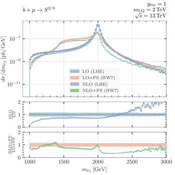
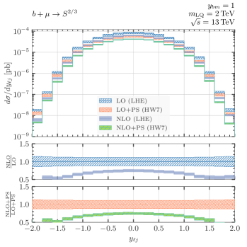
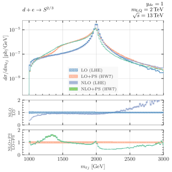
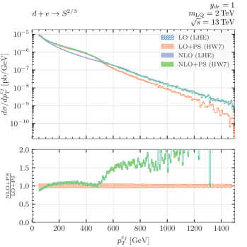
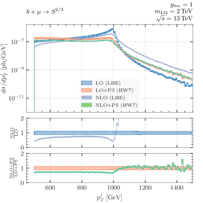
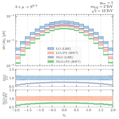
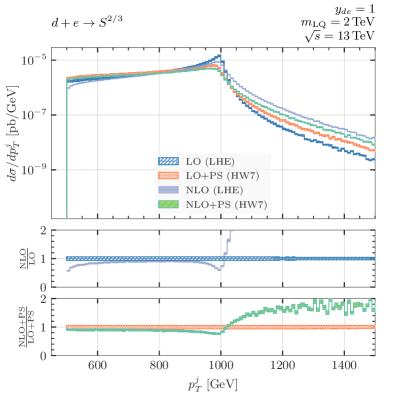
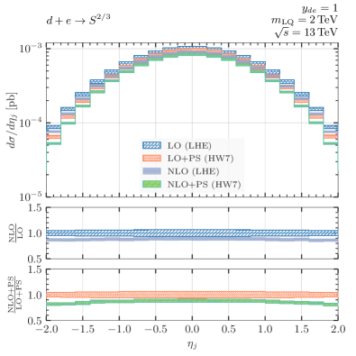
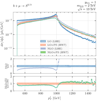
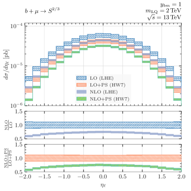
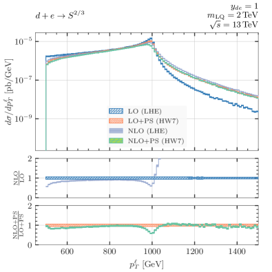
We investigate three benchmark scenarios where the scalar leptoquark is exclusively produced from , , and fusion.777The code provided in the Powheg-Box repository http://powhegbox.mib.infn.it allows studying other benchmarks efficiently. In all cases, the leptoquark charge is set to , while the leptoquark mass is set to TeV for illustration. The Yukawa couplings in Eq. (1) are all set to zero except for the desired quark-lepton flavour combination . The leptoquark is therefore decayed to the same quark-lepton pair. The code automatically computes the total leptoquark decay width using Eq. (15). The energy of the proton beams is set to 6.5 TeV each ( TeV) and the PDF set is LUXlep-NNPDF31_nlo_as_0118_luxqed (central) Buonocore:2020nai .
When running the reconstruction analysis, a perfect detector is assumed with no smearing effects. The high-level objects of interest are the leading- jet and lepton, which typically originate from the leptoquark decay. The jets are built using the anti- algorithm Cacciari:2008gp with as implemented in Fastjet Cacciari:2011ma . The cuts on the transverse momentum and the pseudorapidity are applied, and the hardest jet and lepton are then selected. We also require the total invariant mass of the jet-lepton system to be above 1 TeV and below 4 TeV. Bremsstrahlung recombination was considered for the lepton by adding photons that lie inside a cone of . We see no appreciable difference between the muon and the electron case. This is consistent with the fact that for high-mass objects the quark-electron and quark-muon luminosities are very similar (See Figure 8 in ref. Buonocore:2020nai ), and thus the only substantial difference between muons and electrons is the more significant QED radiation of the latter. So, after recombination, no relevant difference remains. Thus, the case is not shown in the figures since it is indistinguishable from the case. Finite width effects are turned on (see Sec. 2.2).
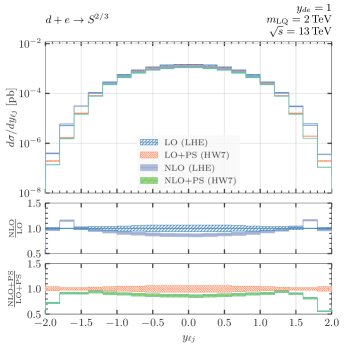
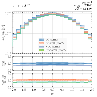
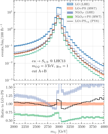
Two million LO and NLO events were processed to generate the plots shown in the Figures 2 and 3. The upper box in each plot displays four lines. The bands show the customary 7-point scale variation uncertainty. The lines labeled LO (LHE), and LO+PS (HW7) are obtained by restricting the event generation with Powheg to leading order and running the analysis before (blue) and after (orange) the parton shower using Herwig. Similarly, the NLO simulations were used for the purple (before PS) and the green (after PS) lines. The two smaller boxes below the main box show the ratio of NLO to LO before and after showering. As illustrated by the plots, the NLO order corrections are sizeable and depend on the kinematics.
The invariant mass and rapidity of the jet-lepton system are shown in Figure 2 in the left and right columns, respectively, for the benchmark scenarios: (top), and (bottom). The jet-lepton system’s invariant mass distributions () show a resonance peak at TeV. The width of the peak before the parton shower is narrow and meets the expectation from the intrinsic leptoquark width in Eq. (15). The effect of the parton shower can be observed as well — the peak position is shifted to a slightly lower value of (), the peak is smaller and considerably broader for the distributions of showered events both at LO and NLO and leans towards lower masses. It is helpful to remark that this effect is mostly due to the fact that, in our NLO calculation, we do not include radiative corrections to the leptoquark decay. Under these circumstances, the final state radiation generated by the Monte Carlo in the leptoquark decay becomes very relevant since it is the only source of jet momentum degradation due to final state radiation outside the jet cone. This causes a sizeable raise of the backward tail and a slight lowering of the forward tail in the invariant mass spectrum. By investigating further this effect, we have found that another contributing factor is the presence of events such that the selected jet is not the one arising from the leptoquark decay. This is more likely to happen in the showered events, since there are more jets in that case. These events tend to inflate the differential distribution below the peak.
When comparing the jet-lepton system’s rapidity plots in Figure 2 (right column), it is worth noticing a broader distribution for the down quark compared to the bottom quark. This behavior stems from the down quark being a valence quark and having a higher probability of carrying a more significant fraction of the proton’s total momentum. Therefore, leptoquarks produced from valence quarks tend to carry more momentum along the beam axis, broadening the shape of the rapidity distribution towards larger values.
Notice also the large difference in the signal rate between the and the case, due to the sea versus valence quark PDF, and to larger NLO corrections in the latter. These features are expected since, as shown in Figure 8 of Ref Greljo:2020tgv for the LQ of charge , the NLO QCD K-factor is close to unity for bottom initiated processes and it does not compensate the negative NLO QED one, which is similar for all quark cases.
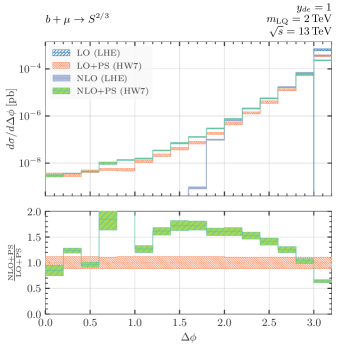
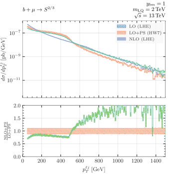
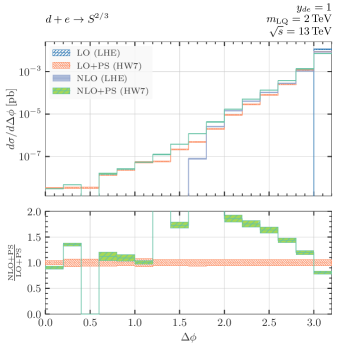
Figure 3 shows the azimuthal angle between the lepton and the jet in the left column, and the transverse momentum of the jet-lepton system in the right column. The between the jet and the lepton in Figure 3 (left column) shows that the two objects are mostly back to back in the azimuthal plane. At LO without parton shower, all events exactly have . The radiation at NLO opens up smaller angles to the distribution. The parton shower populates even smaller angles, but the rate still clearly peaks around as expected. The rapid fall of the LHE band in the plot, near , can be understood as a kinematic effects. As decreases, the transverse momentum of the jet balancing the leptoquark must increase, up to the point when it becomes the hardest jet, and is thus selected as such. The presence of more jets in the shower case can allow instead for a larger boost of the leptoquark, not associated with a single hard jet in acceptance.
The transverse momentum of the jet-lepton system in Figure 3 (right column) is zero for all LO events before the shower. We notice the feature of the distribution for transverse momenta between 200 and 500 GeV, where the showered events have larger cross section, and smaller cross section above 500 GeV. First of all, we have verified that such feature is not present in the distribution of the leptoquark at the “Monte Carlo Truth” level (i.e. the leptoquark in the Monte Carlo just before decay), where a perfect agreement is found between the NLO(LHE) and NLO+PS(HW7) distributions. This is due to the fact that Herwig preserves as much as possible the four momentum of resonances. A good fraction of the effect can be tracked back to the final state radiation from the quark, that as remarked previously, is included only by the shower. Another contribution arises if the hardest jet or the hardest lepton in acceptance are not the ones coming from the leptoquark decay. Of course this happens more easily in showered events.
The plots show that the uncertainty band of the LO predictions vastly underestimates the size of the NLO corrections. There can be considerable shape differences between results at LO and NLO. The NLO corrections are crucial for an accurate description of these distributions. The is helpful to discriminate the resonant leptoquark from the single leptoquark plus lepton production Dorsner:2018ynv which features a hard lepton in the production already at tree-level.
The transverse momentum and the pseudorapidity distributions of the leading jet and lepton are shown in Figure 4 and Figure 5. In all plots, higher-order corrections to the pseudorapidity distributions are slightly flatter than the corresponding ones to the rapidity distribution of the lepton-jet system. Otherwise, they display a similar pattern, and similar comments are in place. As expected, the distributions show a jacobian peak at . The region above the kinematic limit , strictly forbidden at LO in the NWA, is populated by finite-width effects. Starting from NLO, this region also becomes accessible because of extra radiation. This explains the fact that LO (LHE) predictions for are much softer than the other three predictions. Notice that the NLO (LHE) results’ smooth behavior is generated according to the POWHEG Sudakov factor. Showered predictions feature a softer spectrum than NLO (LHE) ones due to final-state radiation. The effect is more pronounced in the case of the leading jet since the radiation probability for additional QED emissions is suppressed by the lower coupling . This explains the rise toward smaller values. Comparing the tail of the leading jet above the peak for the and cases, we observe that, in the latter, NLO+PS(HW7) results present a harder spectrum than LO+PS(HW7) ones, while they overlap in the former. This different behavior can be traced back to the interplay between the initial-state radiation’s hardness and a valence quark’s presence. In fact, in events initiated by a valence quark (that carries a larger fraction of the proton momentum), the first emission is, on average harder, and the NLO+PS generator describes this radiation with higher accuracy than a LO+PS one. On the other hand, in the case of a sea quark, the same configurations feature a softer initial-state radiation and a LO+PS description is sufficient to capture the main effects. For the leading lepton the situation is inverted, with NLO+PS predictions displaying a harder spectrum than LO+PS ones in the case. The physical mechanism is the same described above with the difference that, this time, the initial-state lepton colliding with a sea quark is, on average, more energetic than the one colliding with a valence quark.
3.3 Impact on the projected LHC bounds
The phenomenological studies performed in Buonocore:2020erb ; Haisch:2020xjd disclosed the potential of the resonant leptoquark production through lepton-quark fusion as a competitive search strategy at the LHC, especially for the region of large leptoquark couplings and masses. In that work, the modeling of signal events was based on an approximate LO+PS prediction. The approximation is related to using Pythia8 to shower the LO events. Indeed, Pythia8 does not handle lepton-initiated processes. On the other hand, it supports photons in the initial state. Hence, in that work, the particle labels were suitably manipulated to recognize the process as originating from a photon-quark scattering. In this way, the first radiation generated by the shower is likely to be a colored parton most of the time. At the same time, for a lepton-quark scattering event, the photon splitting process competes with QCD radiation in the backward evolution.888The pdf ratio compensates for the factor of arising from the photon splitting. The resulting mismodeling of the hadronic activity in the event was estimated to have only a mild impact, affecting the prediction for the reconstructed leptoquark mass by roughly Buonocore:2020erb .
In the present work, we have improved the simulation of the signal events in two ways: first, we include the full set of NLO corrections to the leptoquark production process, from now on NLOP, and, second, we match à la POWHEG the NLOP corrections to a modified version of the Herwig7 parton shower Bellm:2019zci that handles lepton initiated processes HW7dev . In the following, we assess the relative impact of these improvements. We consider as a benchmark point a scalar leptoquark of nominal mass TeV, charge and which couples only to electrons and up quarks.
Our main focus is on the reconstructed jet-lepton invariant mass where the leptoquark shows up as a resonance. Additional selection cuts are crucial to tame the SM background. However, they largely affect the shape of the resonant peak and the acceptance of signal events. We consider a simplified version of the fiducial volume defined in Buonocore:2020erb to analyze the main radiative effects. As a basic requirement, dubbed as cut A, we select events with at least one lepton and one jet in the central region of the detector, . We then impose the following set of cuts on leading and subleading leptons/jets, collectively referred to as cut B: GeV, a veto on secondary leptons with GeV and , a veto on secondary jets with GeV and .
In Figure 6, we compare different predictions for the invariant mass distribution of the system composed of the hardest lepton and hardest jet, obtained with samples of signal leptoquark events at different accuracy: LO (blue), LO+PS (HW7) showered with Herwig7 (orange), NLOP Les Houches events as generated with Powheg (gray), NLOP+PS (HW7) the same events showered with Herwig7 (green). The bands correspond to the customary 7-point scale variation. We also report in black the LO+PSγq (PY8) prediction obtained showering the events with Pythia8 after performing the replacement of the initial lepton with a photon as done in Buonocore:2020erb . We leave out multiparton interactions (MPIs) and detector effects from these comparisons to facilitate the discussion. Furthermore, we do not apply any recombination of photons with a close-by lepton.
Let us remind the reader that we computed NLO radiative corrections only to the leptoquark production process, leaving to the parton shower the full description of the radiation from the decay products. For this reason, it is interesting to consider first the case in which we switch off final-state radiation (FSR) in the parton shower, which more closely resembles the radiative content of our NLOP prediction. We start focusing on the plots of the left-hand side of Figure 6, where we apply only the essential requirement cut A. Comparing top and bottom, we observe that the exclusion of FSR leads to much milder parton shower effects. Indeed, the distinctive radiative tail in the bottom plot is entirely due to QCD FSR, which forms a separate second jet softening the leading jet, originated by the quark in the leptoquark decay. Furthermore, we have explicitly verified that photon-to-lepton recombination has a minimal impact on the distribution, confirming that the FSR effects due to QED radiation are less important. When FSR is not included, all predictions are close-by among each other within , except for the one obtained with LO+PS (HW7) generator. This might be due to different shower mechanisms and recoil prescriptions in Pythia8 and Herwig7, whose impact becomes less prominent after performing the matching to the NLOP computation. While this is an interesting topic, its investigation is beyond the aim of the present work, and it is left for a future study.
| cut A (noFSR) | cut A+B (noFSR) | cut A | cut A+B | |
| LO | 0.96 | 0.89 | 0.96 | 0.89 |
| LO+PS (HW7) | 0.98 | 0.48 | 0.98 | 0.28 |
| NLOP | 0.97 | 0.42 | 0.97 | 0.42 |
| NLOP+PS (HW7) | 0.98 | 0.37 | 0.99 | 0.20 |
| LO+PSγq (PY8) | 0.97 | 0.51 | 0.98 | 0.29 |
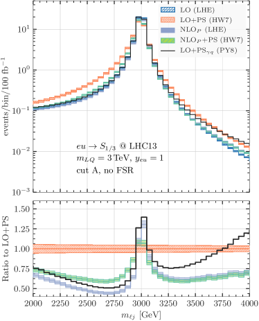
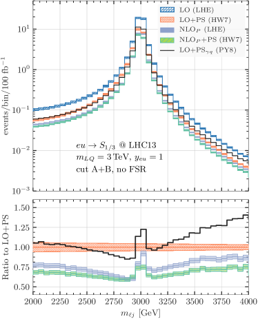
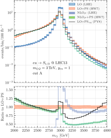
We turn to the more interesting situation in which we apply the combination of cuts cut A+B. The results are shown in the plots of the right-hand side of Figure 6, excluding (top) or not (bottom) FSR radiation. Since the cuts are tailored to enhance Born-like configurations, the LO prediction remains in practice untouched. On the other hand, the veto on secondary leptons and jets vastly reduces all the other predictions, see Tab 3. In addition, the radiative tail seen in the more inclusive setup is effectively cut out. In particular, when FSR is excluded (top right), we observe that the result obtained with the NLOP+PS (HW7) generator only mildly differs from the NLOP one, meaning that only the first few emissions are relevant for the computation of the acceptance. The radiation from the decay products further reduces the acceptance. Since the NLOP computation does not contain such effects, it fails to describe the total result. Instead, the LO+PS predictions and the more accurate NLOP+PS one includes radiative effects from the decay as modeled by FSR of the parton shower (bottom right).
The main results regarding the A+B cuts can be summarised as follows:
-
•
NLOP provides an estimate of the acceptance that, however, misses the effects due to radiation from the decay products;
-
•
LO+PSγq (PY8) and LO+PS (HW7) give results in reasonable agreement among each other, with very mild differences of about . Nonetheless, we notice that this result might be accidental given that we observe substantial differences in the mass spectrum predicted by the two generators when FSR is turning off. This issue seems alleviated after the NLO matching, as the NLOP+PS(HW7) and LO+PSγq (PY8 display an overall better agreement in shape. We believe that this is a further motivation for the experts in parton showers to pursue the study of lepton initiated processes in proton-proton collisions;
-
•
by comparing with the NLOP, FSR radiation contributes to the reduction of the acceptance of a further , see also Tab. 3;
-
•
the most accurate NLOP+PS prediction leads to a further reduction of the acceptance of about with respect to LO+PS ones. This can be explained by the fact that the former includes the exact matrix element for the first emission in production. As a result, we expect the limits on the leptoquark couplings shown in Figure 3 of Buonocore:2020erb to relax by about .
It is well known that parton showers usually provide a better description of FSR radiation than ISR. Therefore, one may expect that the NLOP+PS description computed in this work already captures the main radiative effects. Nonetheless, given the importance of FSR in computing the acceptance, a natural extension of the present work would be to match the NLO computation for all possible resonant and non-resonant quark-lepton processes to the parton shower, thus including radiation from all legs and (or) resonant intermediate states.
3.4 The case study: leptoquark
To illustrate the usage of the code for a particular UV model, we add to the SM an additional scalar field transforming in the anti-fundamental of and the adjoint of with the hypercharge , known as the leptoquark Dorsner:2016wpm . In the unbroken phase, the renormalisable Lagrangian describing the couplings of to the SM fermions reads
| (16) |
where are the Pauli matrices, , stands for charge conjugation, and are leptoquark components in the space. The matrices and are generic matrices in flavour space. The summation over flavours is assumed. It is easy to argue that dangerous diquark couplings are absent due to an (approximate) baryon number conservation.999This can be achieved, for example, in some GUT models where is embedded in or irreducible representation Senjanovic:1982ex ; Dorsner:2017ufx . Another example is to gauge a lepton flavour non-universal under which is charged such that completely forbids proton decay Davighi:2022qgb .
The left-handed quark and lepton doublets, and , are assumed to be in the down-quark and charged-lepton mass basis, respectively. After the electroweak symmetry breaking, the relevant interactions of the electromagnetic charge eigenstates , , and , in the notation of Eq. (1), read
| (17) |
where and stand for the three up- and down-type quarks, while () stands for the three charged leptons (neutrinos), and
| (18) | ||||
| (19) |
where is the Pontecorvo–Maki–Nakagawa–Sakata mixing matrix, and is the Cabibbo-Kobayashi-Maskawa mixing matrix. The gauge symmetry predicts the three states to be nearly mass-degenerate. Potentially significant contributions to the mass splitting are constrained by the electroweak precision tests Dorsner:2016wpm . This is, of course, very important for the direct searches at the LHC, predicting multiple degenerate resonances.
Since the neutrino PDF in the proton is vanishing (at the order in perturbation theory we are working at101010It can be generated with a mechanism similar to the lepton PDF, going through a rather than a photon, but, unlike the lepton case, the logarithmic enhancement is missing.), proton collisions can produce only the states with charges and in the quark-lepton fusion. However, various decay channels are generally open (including neutrinos), and the branching ratios depend on the flavour structure of .
When the leptoquark flavour matrix has an anarchic structure, the low-energy flavour physics observables set a lower limit on to be far above the TeV scale, see Dorsner:2016wpm ; Isidori:2010kg . A consistent scenario should therefore exhibit flavour protection. For simplicity, we assume that the leptoquark carries a global quark and lepton charges, where and denote a particular quark and lepton flavour combination, such that the only allowed coupling becomes
| (20) |
where is a complex number. For example, the case in which the leptoquark is charged under the global symmetry implies that the only non-vanishing entry in is the entry, . Neglecting neutrino masses, which is an excellent approximation at relevant energies, this symmetry is broken only by the CKM mixing matrices. In this limit, the flavour-changing contributions in the quark sector are suppressed by the smallness of the off-diagonal CKM elements while charged lepton flavour is exactly conserved. For the direct searches at the LHC, the CKM can safely be approximated with the unit matrix.
The bottomline of these assumptions is that the leptoquark interacts dominantly with a single generation of quarks and a single generation of leptons. In the following, we will study all six quark flavour cases separately. Since the lepton PDF are similar across different flavours, we will consider only the coupling to muons for simplicity.111111An example of a particularly motivated flavour structure in the quark sector is flavour symmetry under which the third generation is invariant while the light generations form doublets Barbieri:2011ci ; Faroughy:2020ina ; Greljo:2022cah . This symmetry is an excellent approximate symmetry of the SM Yukawa sector. In the leptonic sector, the symmetry can result accidentally from a lepton non-universal gauge symmetry Greljo:2021xmg ; Greljo:2021npi ; Davighi:2020qqa ; Hambye:2017qix ; Davighi:2022qgb ; Heeck:2022znj . Thus, in the exact symmetry limit, only the entry, , is allowed. Figure 7 shows this case with the orange curve, while the projections at future colliders (in other channels) were also considered in Azatov:2022itm .
With all this, the LO decay widths of and states are given as
| (21) | ||||
| (22) |
where we sum over quark and lepton flavour indices. In the case of global symmetry, , with depending on the quark generation which couples to the leptoquark.
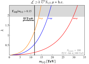
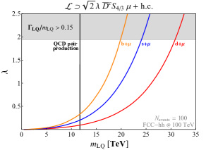
Let us finally discuss the importance of the resonant leptoquark production at the FCC-hh collider operating at proton-proton center of mass energy, with the luminosity of . We do not aim to derive precise projections since a complete analysis, including the signal and background simulations, is clearly beyond the scope of this work. Instead, a simple comparison with the QCD pair production can already be made using the inclusive cross sections from Section 3.1 and predicted branching ratios to determine the parameter space for which one can produce more than 100 events. Even though it is a naive estimate, since the SM background is subleading in the high-energy bins (as proved in Buonocore:2020erb ) and the signal is resonant, we expect 100 events to guarantee a discovery. A detailed projection study for the QCD pair production mechanism Allanach:2019zfr gives a result very close to this criteria.
Figure 7 illustrates the main point. The plot on the left (right) side is for the () state. The solid black line is for the QCD pair production, while the red, blue, and orange lines are for different quark generations in increasing order. The regions left to the lines is where the FCC-hh can produce more than 100 events. Finally, the grey shaded region predicts a broad resonance (). The plots show large portions of parameter space for which the resonant leptoquark production channel offers a unique window for discovery. This finding motivates a comprehensive projection study for future work.
4 Conclusions
Leptoquarks at the TeV scale are predicted in various settings beyond the SM, such as non-minimal composite Higgs models, -parity violating supersymmetric models, extended gauge symmetries, and others. Leptoquark extensions of the SM have recently been under the spotlight as promising candidates to address various flavour anomalies. As a result, ATLAS and CMS collaborations are investing increasingly more resources to search for these particles. Direct discovery of a leptoquark would have profound implications for the paradigm of quark-lepton unification at shorter distances.
Precise determination of lepton densities inside the proton Buonocore:2020nai revealed a novel path for leptoquark production at the LHC. Despite the smallness of the lepton PDF, a direct quark-lepton fusion at the partonic level is the most sensitive production channel for large leptoquark couplings, thanks to the resonant enhancement. Indeed, the first phenomenological studies show that large portions of the leptoquark model’s parameter space can uniquely be probed through this channel Buonocore:2020erb . This study, however, relies on tree-level calculations and a crude estimate of the lepton shower effects that were not developed at the time. The first calculation at NLO Greljo:2020tgv , albeit limited to the inclusive cross sections, showed an interesting pattern of QCD and QED corrections which are similar in size. However, the full NLO description of the process, including differential distributions, was still missing.
In this work, we develop the first Monte Carlo event generator for precision studies of the resonant leptoquark production at hadron colliders. In Section 2.1 we present the Powheg-Box-Res implementation of the process at NLO matched to parton shower, including the lepton shower, which has recently become available in Herwig. Section 2.2 discusses leptoquark decays and the treatment of the resonance line shape. Our code allows for a full-fledged simulation of the process and is flexible enough to include all renormalisable scalar leptoquark models with arbitrary flavour structures Dorsner:2016wpm . We leave for future work the implementation of the vector leptoquark models.
We validate the code by reproducing the NLO inclusive cross sections at the LHC Greljo:2020tgv and provide new results for the FCC-hh (see Section 3.1). The unique advantage of our Powheg-Box-Res implementation is the possibility to study arbitrary differential distributions. In Section 3.2, we comprehensively investigate the phenomenologically relevant observables, such as the jet-lepton azimuthal distance and the system’s invariant mass, , and rapidity. As an illustration, in Figures 2 and 3 we show these distributions for three different benchmark points, at LO or NLO and with or without PS. We conclude that higher-order corrections are kinematics-dependent and should be adequately incorporated. In Section 3.3, we study the importance of improved signal predictions on the (HL-)LHC projections reported in Buonocore:2020erb . We closely follow the cut flow analysis of Buonocore:2020erb to find an overestimation of the acceptance of up to .
To illustrate the potential of the FCC-hh, in Section 3.4 we study a concrete model, the scalar leptoquark. Figure 7 shows the leptoquark coupling as a function of mass needed to produce 100 events. We find that the resonant production mechanism can potentially probe uncharted parameter space beyond the reach of QCD pair production for all quark flavours (including the top quark). Our simplified analysis motivates a detailed projections study at the FCC-hh, including the background simulation, which is left for future work.
To conclude, this work paves the way for the first experimental searches and further phenomenological studies of the resonant leptoquark production at the LHC (and beyond). The latest addition to the leptoquark toolbox is made publicly available at the website http://powhegbox.mib.infn.it.
Acknowledgements
We thank Silvia Ferrario Ravasio for clarifying issues with Herwig. The code for the computation of the running in the project repository was taken from the Hoppet code Salam:2008qg . The work of AG has received funding from the Swiss National Science Foundation (SNF) through the Eccellenza Professorial Fellowship “Flavor Physics at the High Energy Frontier” project number 186866. The work of AG and NS is also partially supported by the European Research Council (ERC) under the European Union’s Horizon 2020 research and innovation programme, grant agreement 833280 (FLAY). PN acknowledges the Humboldt foundation for support and the Max Planck Institute for Physics for hospitality. The work of LB is supported by the UZH Postdoc Grant Forschungskredit K-72324-03.
Appendix A Instructions to run the code
The purpose of this appendix is to provide a brief guide to run the code. By the end of this section the reader should be able to reproduce the plots such as the ones in Figures 2, 3, 4 and 5. The first step is to download the Powheg-Box-Res and then get the process LQ-s-chan from the svn repository svn://powhegbox.mib.infn.it/trunk/User-Processes-RES/LQ-s-chan. At the time of writing Powheg-Box-Res is at revision 3967.
The Makefile may need a few modifications. At the beginning choose the compiler and check that the commands to invoke the compiler (F77, CC and CXX) match your system. On new MacOS gcc and g++ by default point to clang and clang++. This can lead to problems when linking against libraries built with the actual GNU Compiler Collection (gcc).121212It is possible to run this on the new Apple Silicon processors if all packages are built using homebrews gcc and gfortran. LHAPDF is used to access the lepton PDFs LUXlep-NNPDF31_nlo_as_0118_luxqed. Therefore, the lhapdf-config executable should be in the path. Set the variable RES to the path of Powheg-Box-Res following the examples in the file. Now it should be possible to build both targets (pwhg_main and lhef_analysis).
In order to shower the events one needs to download the appropriate version of Herwig7. In the folder HerwigInstallation one can find a simple installation script. It can be run directly, or used as a sequence of instructions to install Herwig7. The next step is to build the Herwig interface. To do so edit the Makefile in the folder HerwigInterface. The variable PROCDIR has to be set to the path of the LQ-Res-Prod folder. Again set the path to Powheg-Box-Res and check whether the herwig-config and thepeg-config executables are in the path. Also, set the correct path to the HepMC2 library. After building the interface return to the project’s main folder. Finally navigate to the folder’s scripts and build the two executables mergedata and pastegnudata. Move them to a directory in the path. Everything needed to compute the histograms should now be compiled.
To quickly check whether the code is yielding results open the script run.sh and adjust the variables ncores and nprocesses to the system. To execute the code create two directories, one for the LO and one for the NLO computation. Copy the content of the folder run-master to both folders. Now the input cards for Powheg-Box-Res and Herwig should be present among some scripts to run the code on multiple cores. In the LO folder rename powheg.input-save-LO to powheg.input-save. Among many parameters that control the behaviour of Powheg-Box-Res the mass and charge of the desired leptoquark is specified in this file. The mass and the charge of the leptoquark, as well as, the quark and lepton flavours, can be set. The latter is done by enabling the coupling for the corresponding family of quarks and leptons. The flavour of the quarks is determined by the charge of the leptoquark. If the number of events was changed in the POWHEG input card, the corresponding line in the Herwig input card Herwig.in should be modified.
To run the code, modify the lines controlling the number of cores and processes in the run-parallel.sh script and execute it. This script will run multiple instances of Powheg-Box-Res and create the Les Houches events files. For the analysis, execute the runlhe.sh script. The parton shower and its analysis is done by running the script hw7.sh. Move the files with the top-extensions from the HerwigRun directory up to the current directory and run refine.sh combine the data from all processes. The same procedure can be repeated for the NLO case. To plot the histograms create a new directory and copy the python scripts to it. Set the variable RUNDIRLO and RUNDIRNLO to the directories containing the tables created with refine.sh. Run the python script plots.py to obtain the histograms.
References
- (1) J. C. Pati and A. Salam, Lepton Number as the Fourth Color, Phys. Rev. D 10 (1974) 275–289.
- (2) H. Georgi and S. L. Glashow, Unity of All Elementary Particle Forces, Phys. Rev. Lett. 32 (1974) 438–441.
- (3) H. Fritzsch and P. Minkowski, Unified Interactions of Leptons and Hadrons, Annals Phys. 93 (1975) 193–266.
- (4) I. Doršner, S. Fajfer, A. Greljo, J. F. Kamenik and N. Košnik, Physics of leptoquarks in precision experiments and at particle colliders, Phys. Rept. 641 (2016) 1–68, [1603.04993].
- (5) B. Gripaios, Composite Leptoquarks at the LHC, JHEP 02 (2010) 045, [0910.1789].
- (6) J. Fuentes-Martín and P. Stangl, Third-family quark-lepton unification with a fundamental composite Higgs, Phys. Lett. B 811 (2020) 135953, [2004.11376].
- (7) R. Barbieri and A. Tesi, -decay anomalies in Pati-Salam SU(4), Eur. Phys. J. C 78 (2018) 193, [1712.06844].
- (8) F. Sannino, P. Stangl, D. M. Straub and A. E. Thomsen, Flavor Physics and Flavor Anomalies in Minimal Fundamental Partial Compositeness, Phys. Rev. D 97 (2018) 115046, [1712.07646].
- (9) D. Marzocca, Addressing the B-physics anomalies in a fundamental Composite Higgs Model, JHEP 07 (2018) 121, [1803.10972].
- (10) G. F. Giudice and R. Rattazzi, R-parity violation and unification, Phys. Lett. B 406 (1997) 321–327, [hep-ph/9704339].
- (11) C. Csaki, Y. Grossman and B. Heidenreich, MFV SUSY: A Natural Theory for R-Parity Violation, Phys. Rev. D 85 (2012) 095009, [1111.1239].
- (12) W. Altmannshofer, P. S. B. Dev, A. Soni and Y. Sui, Addressing R, R, muon and ANITA anomalies in a minimal -parity violating supersymmetric framework, Phys. Rev. D 102 (2020) 015031, [2002.12910].
- (13) H. K. Dreiner, V. M. Lozano, S. Nangia and T. Opferkuch, Lepton PDFs and Multipurpose Single Lepton Searches at the LHC, 2112.12755.
- (14) L. Di Luzio, A. Greljo and M. Nardecchia, Gauge leptoquark as the origin of B-physics anomalies, Phys. Rev. D 96 (2017) 115011, [1708.08450].
- (15) M. Bordone, C. Cornella, J. Fuentes-Martin and G. Isidori, A three-site gauge model for flavor hierarchies and flavor anomalies, Phys. Lett. B 779 (2018) 317–323, [1712.01368].
- (16) A. Greljo and B. A. Stefanek, Third family quark–lepton unification at the TeV scale, Phys. Lett. B 782 (2018) 131–138, [1802.04274].
- (17) B. Fornal, S. A. Gadam and B. Grinstein, Left-Right SU(4) Vector Leptoquark Model for Flavor Anomalies, Phys. Rev. D 99 (2019) 055025, [1812.01603].
- (18) J. Heeck and D. Teresi, Pati-Salam explanations of the B-meson anomalies, JHEP 12 (2018) 103, [1808.07492].
- (19) C. Cornella, J. Fuentes-Martin and G. Isidori, Revisiting the vector leptoquark explanation of the B-physics anomalies, JHEP 07 (2019) 168, [1903.11517].
- (20) M. Blanke and A. Crivellin, Meson Anomalies in a Pati-Salam Model within the Randall-Sundrum Background, Phys. Rev. Lett. 121 (2018) 011801, [1801.07256].
- (21) S. Balaji and M. A. Schmidt, Unified SU(4) theory for the and anomalies, Phys. Rev. D 101 (2020) 015026, [1911.08873].
- (22) BaBar collaboration, J. P. Lees et al., Measurement of an Excess of Decays and Implications for Charged Higgs Bosons, Phys. Rev. D 88 (2013) 072012, [1303.0571].
- (23) Belle collaboration, S. Hirose et al., Measurement of the lepton polarization and in the decay , Phys. Rev. Lett. 118 (2017) 211801, [1612.00529].
- (24) LHCb collaboration, R. Aaij et al., Measurement of the ratio of branching fractions , Phys. Rev. Lett. 115 (2015) 111803, [1506.08614].
- (25) LHCb collaboration, R. Aaij et al., Test of lepton universality using decays, Phys. Rev. Lett. 113 (2014) 151601, [1406.6482].
- (26) LHCb collaboration, R. Aaij et al., Test of lepton universality with decays, JHEP 08 (2017) 055, [1705.05802].
- (27) LHCb collaboration, R. Aaij et al., Measurement of Form-Factor-Independent Observables in the Decay , Phys. Rev. Lett. 111 (2013) 191801, [1308.1707].
- (28) LHCb collaboration, R. Aaij et al., Angular analysis of the decay using 3 fb-1 of integrated luminosity, JHEP 02 (2016) 104, [1512.04442].
- (29) LHCb collaboration, R. Aaij et al., Search for lepton-universality violation in decays, Phys. Rev. Lett. 122 (2019) 191801, [1903.09252].
- (30) ATLAS collaboration, G. Aad et al., Search for new phenomena in collisions in final states with tau leptons, b-jets, and missing transverse momentum with the ATLAS detector, Phys. Rev. D 104 (2021) 112005, [2108.07665].
- (31) ATLAS collaboration, G. Aad et al., Search for pair production of third-generation scalar leptoquarks decaying into a top quark and a -lepton in collisions at = 13 TeV with the ATLAS detector, JHEP 06 (2021) 179, [2101.11582].
- (32) ATLAS collaboration, M. Aaboud et al., Searches for third-generation scalar leptoquarks in = 13 TeV pp collisions with the ATLAS detector, JHEP 06 (2019) 144, [1902.08103].
- (33) ATLAS collaboration, G. Aad et al., Search for pair production of scalar leptoquarks decaying into first- or second-generation leptons and top quarks in proton–proton collisions at = 13 TeV with the ATLAS detector, Eur. Phys. J. C 81 (2021) 313, [2010.02098].
- (34) ATLAS collaboration, G. Aad et al., Search for pairs of scalar leptoquarks decaying into quarks and electrons or muons in = 13 TeV collisions with the ATLAS detector, JHEP 10 (2020) 112, [2006.05872].
- (35) CMS collaboration, A. M. Sirunyan et al., Search for singly and pair-produced leptoquarks coupling to third-generation fermions in proton-proton collisions at s=13 TeV, Phys. Lett. B 819 (2021) 136446, [2012.04178].
- (36) CMS collaboration, A. M. Sirunyan et al., Search for leptoquarks coupled to third-generation quarks in proton-proton collisions at 13 TeV, Phys. Rev. Lett. 121 (2018) 241802, [1809.05558].
- (37) CMS collaboration, A. M. Sirunyan et al., Constraints on models of scalar and vector leptoquarks decaying to a quark and a neutrino at 13 TeV, Phys. Rev. D 98 (2018) 032005, [1805.10228].
- (38) CMS collaboration, A. Tumasyan et al., Inclusive nonresonant multilepton probes of new phenomena at =13 TeV, Phys. Rev. D 105 (2022) 112007, [2202.08676].
- (39) CMS collaboration, A. Tumasyan et al., Search for new particles in events with energetic jets and large missing transverse momentum in proton-proton collisions at = 13 TeV, JHEP 11 (2021) 153, [2107.13021].
- (40) J. Blumlein, E. Boos and A. Kryukov, Leptoquark pair production in hadronic interactions, Z. Phys. C 76 (1997) 137–153, [hep-ph/9610408].
- (41) M. Kramer, T. Plehn, M. Spira and P. M. Zerwas, Pair production of scalar leptoquarks at the Tevatron, Phys. Rev. Lett. 79 (1997) 341–344, [hep-ph/9704322].
- (42) M. Kramer, T. Plehn, M. Spira and P. M. Zerwas, Pair production of scalar leptoquarks at the CERN LHC, Phys. Rev. D 71 (2005) 057503, [hep-ph/0411038].
- (43) B. Diaz, M. Schmaltz and Y.-M. Zhong, The leptoquark Hunter’s guide: Pair production, JHEP 10 (2017) 097, [1706.05033].
- (44) C. Borschensky, B. Fuks, A. Kulesza and D. Schwartländer, Scalar leptoquark pair production at hadron colliders, Phys. Rev. D 101 (2020) 115017, [2002.08971].
- (45) B. C. Allanach, T. Corbett and M. Madigan, Sensitivity of Future Hadron Colliders to Leptoquark Pair Production in the Di-Muon Di-Jets Channel, Eur. Phys. J. C 80 (2020) 170, [1911.04455].
- (46) C. Borschensky, B. Fuks, A. Jueid and A. Kulesza, Scalar leptoquarks at the LHC and flavour anomalies: a comparison of pair-production modes at NLO-QCD, 2207.02879.
- (47) I. Doršner and A. Greljo, Leptoquark toolbox for precision collider studies, JHEP 05 (2018) 126, [1801.07641].
- (48) A. Alves, O. Eboli and T. Plehn, Stop lepton associated production at hadron colliders, Phys. Lett. B 558 (2003) 165–172, [hep-ph/0211441].
- (49) J. B. Hammett and D. A. Ross, NLO Leptoquark Production and Decay: The Narrow-Width Approximation and Beyond, JHEP 07 (2015) 148, [1501.06719].
- (50) T. Mandal, S. Mitra and S. Seth, Single Productions of Colored Particles at the LHC: An Example with Scalar Leptoquarks, JHEP 07 (2015) 028, [1503.04689].
- (51) D. A. Faroughy, A. Greljo and J. F. Kamenik, Confronting lepton flavor universality violation in B decays with high- tau lepton searches at LHC, Phys. Lett. B 764 (2017) 126–134, [1609.07138].
- (52) A. Greljo and D. Marzocca, High- dilepton tails and flavor physics, Eur. Phys. J. C 77 (2017) 548, [1704.09015].
- (53) M. Schmaltz and Y.-M. Zhong, The leptoquark Hunter’s guide: large coupling, JHEP 01 (2019) 132, [1810.10017].
- (54) J. Fuentes-Martin, A. Greljo, J. Martin Camalich and J. D. Ruiz-Alvarez, Charm physics confronts high-pT lepton tails, JHEP 11 (2020) 080, [2003.12421].
- (55) A. Greljo, J. Martin Camalich and J. D. Ruiz-Álvarez, Mono- Signatures at the LHC Constrain Explanations of -decay Anomalies, Phys. Rev. Lett. 122 (2019) 131803, [1811.07920].
- (56) D. Marzocca, U. Min and M. Son, Bottom-Flavored Mono-Tau Tails at the LHC, JHEP 12 (2020) 035, [2008.07541].
- (57) M. J. Baker, J. Fuentes-Martín, G. Isidori and M. König, High- signatures in vector–leptoquark models, Eur. Phys. J. C 79 (2019) 334, [1901.10480].
- (58) L. Allwicher, D. A. Faroughy, F. Jaffredo, O. Sumensari and F. Wilsch, Drell-Yan Tails Beyond the Standard Model, 2207.10714.
- (59) J. Ohnemus, S. Rudaz, T. F. Walsh and P. M. Zerwas, Single leptoquark production at hadron colliders, Phys. Lett. B 334 (1994) 203–207, [hep-ph/9406235].
- (60) L. Buonocore, P. Nason, F. Tramontano and G. Zanderighi, Leptons in the proton, JHEP 08 (2020) 019, [2005.06477].
- (61) L. Buonocore, U. Haisch, P. Nason, F. Tramontano and G. Zanderighi, Lepton-Quark Collisions at the Large Hadron Collider, Phys. Rev. Lett. 125 (2020) 231804, [2005.06475].
- (62) U. Haisch and G. Polesello, Resonant third-generation leptoquark signatures at the Large Hadron Collider, JHEP 05 (2021) 057, [2012.11474].
- (63) A. Greljo and N. Selimovic, Lepton-Quark Fusion at Hadron Colliders, precisely, JHEP 03 (2021) 279, [2012.02092].
- (64) G. Bewick, S. Ferrario Ravasio, P. Richardson and M. H. Seymour, Initial state radiation in the Herwig 7 angular-ordered parton shower, JHEP 01 (2022) 026, [2107.04051].
- (65) FCC collaboration, A. Abada et al., FCC-hh: The Hadron Collider: Future Circular Collider Conceptual Design Report Volume 3, Eur. Phys. J. ST 228 (2019) 755–1107.
- (66) S. Alioli, P. Nason, C. Oleari and E. Re, A general framework for implementing NLO calculations in shower Monte Carlo programs: the POWHEG BOX, JHEP 06 (2010) 043, [1002.2581].
- (67) Z. Kunszt and W. J. Stirling, QCD corrections and the leptoquark interpretation of the HERA high Q**2 events, Z. Phys. C 75 (1997) 453–463, [hep-ph/9703427].
- (68) T. Plehn, H. Spiesberger, M. Spira and P. M. Zerwas, Formation and decay of scalar leptoquarks / squarks in e p collisions, Z. Phys. C 74 (1997) 611–614, [hep-ph/9703433].
- (69) T. Sjöstrand, S. Ask, J. R. Christiansen, R. Corke, N. Desai, P. Ilten, S. Mrenna, S. Prestel, C. O. Rasmussen and P. Z. Skands, An introduction to PYTHIA 8.2, Comput. Phys. Commun. 191 (2015) 159–177, [1410.3012].
- (70) J. Bellm et al., Herwig 7.2 release note, Eur. Phys. J. C 80 (2020) 452, [1912.06509].
- (71) P. Nason, A New method for combining NLO QCD with shower Monte Carlo algorithms, JHEP 11 (2004) 040, [hep-ph/0409146].
- (72) https://phab.hepforge.org/source/herwighg.
- (73) L. Buonocore, P. Nason, F. Tramontano and G. Zanderighi, Photon and leptons induced processes at the LHC, JHEP 12 (2021) 073, [2109.10924].
- (74) M. A. Gigg and P. Richardson, Simulation of Finite Width Effects in Physics Beyond the Standard Model, 0805.3037.
- (75) S. Frixione, Z. Kunszt and A. Signer, Three jet cross-sections to next-to-leading order, Nucl. Phys. B 467 (1996) 399–442, [hep-ph/9512328].
- (76) Particle Data Group collaboration, R. L. Workman and Others, Review of Particle Physics, PTEP 2022 (2022) 083C01.
- (77) NNPDF collaboration, R. D. Ball et al., Parton distributions from high-precision collider data, Eur. Phys. J. C 77 (2017) 663, [1706.00428].
- (78) B. Fornal, A. V. Manohar and W. J. Waalewijn, Electroweak Gauge Boson Parton Distribution Functions, JHEP 05 (2018) 106, [1803.06347].
- (79) C. W. Bauer and B. R. Webber, Polarization Effects in Standard Model Parton Distributions at Very High Energies, JHEP 03 (2019) 013, [1808.08831].
- (80) M. Cacciari, G. P. Salam and G. Soyez, The anti- jet clustering algorithm, JHEP 04 (2008) 063, [0802.1189].
- (81) M. Cacciari, G. P. Salam and G. Soyez, FastJet User Manual, Eur. Phys. J. C 72 (2012) 1896, [1111.6097].
- (82) G. Senjanovic and A. Sokorac, Light Leptoquarks in SO(10), Z. Phys. C 20 (1983) 255.
- (83) I. Doršner, S. Fajfer, D. A. Faroughy and N. Košnik, The role of the GUT leptoquark in flavor universality and collider searches, JHEP 10 (2017) 188, [1706.07779].
- (84) J. Davighi, A. Greljo and A. E. Thomsen, Leptoquarks with Exactly Stable Protons, 2202.05275.
- (85) G. Isidori, Y. Nir and G. Perez, Flavor Physics Constraints for Physics Beyond the Standard Model, Ann. Rev. Nucl. Part. Sci. 60 (2010) 355, [1002.0900].
- (86) R. Barbieri, G. Isidori, J. Jones-Perez, P. Lodone and D. M. Straub, and Minimal Flavour Violation in Supersymmetry, Eur. Phys. J. C 71 (2011) 1725, [1105.2296].
- (87) D. A. Faroughy, G. Isidori, F. Wilsch and K. Yamamoto, Flavour symmetries in the SMEFT, JHEP 08 (2020) 166, [2005.05366].
- (88) A. Greljo, A. Palavrić and A. E. Thomsen, Adding Flavor to the SMEFT, 2203.09561.
- (89) A. Greljo, P. Stangl and A. E. Thomsen, A model of muon anomalies, Phys. Lett. B 820 (2021) 136554, [2103.13991].
- (90) A. Greljo, Y. Soreq, P. Stangl, A. E. Thomsen and J. Zupan, Muonic force behind flavor anomalies, JHEP 04 (2022) 151, [2107.07518].
- (91) J. Davighi, M. Kirk and M. Nardecchia, Anomalies and accidental symmetries: charging the scalar leptoquark under Lμ Lτ, JHEP 12 (2020) 111, [2007.15016].
- (92) T. Hambye and J. Heeck, Proton decay into charged leptons, Phys. Rev. Lett. 120 (2018) 171801, [1712.04871].
- (93) J. Heeck and A. Thapa, Explaining lepton-flavor non-universality and self-interacting dark matter with , Eur. Phys. J. C 82 (2022) 480, [2202.08854].
- (94) A. Azatov, F. Garosi, A. Greljo, D. Marzocca, J. Salko and S. Trifinopoulos, New Physics in : FCC-hh or a Muon Collider?, 2205.13552.
- (95) G. P. Salam and J. Rojo, A Higher Order Perturbative Parton Evolution Toolkit (HOPPET), Comput. Phys. Commun. 180 (2009) 120–156, [0804.3755].