ABSTRACT: The discovery of gas in Groningen in 1959 has been a massive boon to the Dutch economy. From the 1990s onwards though, gas production has led to induced seismicity. In this paper, we carry out a comprehensive exploratory analysis of the spatio-temporal earthquake catalogue. We develop a non-parametric adaptive kernel smoothing technique to estimate the spatio-temporal hazard map and to interpolate monthly well-based gas production statistics. Second- and higher-order inhomogeneous summary statistics are used to show that the state of the art rate-and-state models for the prediction of seismic hazard fail to capture inter-event interaction in the earthquake catalogue. Based on these findings, we suggest a modified rate-and-state model that also takes into account changes in gas production volumes and uncertainty in the pore pressure field.

Keywords: adaptive bandwidth selection, induced seismicity, inhomogeneous summary statistics, kernel smoothing, pore pressure, spatio-temporal point process.

1 Introduction

In 1959, a large gas field was discovered in Groningen, a province in the North of The Netherlands. Its recoverable gas volume has been estimated at around $2,900$ billion Normal cubic metres (Nbcm). The extraction rate has varied considerably over the years. After a modest start, large amounts were being produced annually during the early 1970s rising to about $85$ Nbcm in 1976. During the next decade, the production volumes tended to decrease, followed by somewhat higher values during the first half of the 1990s. Production fell again during the second half of the decade, before rising in the new millennium to over $53$ bcm in 2013. From the 1990s earthquakes were being registered in the previously tectonically inactive Groningen region. Especially the one near Huizinge in August 2012 with a magnitude of $3.6$ led to a public demand for a reduction of gas production volumes. The government reacted with legislation to phase out gas extraction and, by 2020, production had fallen to less than $8$ Nbcm.

Numerous studies on the Groningen field have been conducted. For example, Geerdink [14] models the times in between earthquakes in terms of the cumulative and annual production rates, pressure, subsidence and fault zones. More recent examples of such a study include Post et al. [23] and Trampert et al. [26]. Van Hove et al. [16] propose a Poisson auto-regression model for the annual hazard maps in terms of subsidence, fault lines and gas extraction in previous years. Both Hettema et al. [15] and Vlek [27] explore the temporal development of seismicity in Groningen by proposing a linear model for the relation between the number of earthquakes over specific periods and gas production volumes. Sijacic et al. [25] focus on the detection of changes in the rate of a temporal Poisson point process by Bayesian and frequentist methods. Bourne et al. [3] modify Ogata’s space-time model [22] to include changes in stress level and estimate the probability of fault failures. Other papers, notably Candela et al. [4], Dempsey and Suckale [10] and Richter et al. [24], discuss the modelling of seismicity in relation to stress changes based on a differential equation and embed these in a space-time Poisson point process.

In a previous paper [2], we investigated the temporal development of seismicity in Groningen including data up to 2020 using cumulative and recent gas production as dependent variables in a regression model. We concluded that a decrease in production leads to decreased seismicity. Here, we extend the analysis to take into account spatial variations. First, we calculate non-parametric estimates for the spatio-temporal hazard map by means of an adaptive kernel smoother (cf. Abramson [1], Davies et al. [9] and Van Lieshout [20]) and generalise the bandwidth selection approach suggested by Van Lieshout [20] to the space-time domain. Using this map, we investigate whether a Poisson point process model would suffice. Employing inhomogeneous summary statistics, we find that there is interaction which cannot be accounted for by Poisson models, including the state of the art rate-and-state models in Candela et al. [4], Dempsey and Suckale [10] and Richter et al. [24]. Since rate-and-state models rely on differential equations for changes in Coulomb stress or, equivalently, pore pressure, we shift our attention to pressure and production data in the public domain. The production values are measured monthly at wells whereas pressure is gauged at irregular times at some wells as well as at several observation and seismic monitoring stations. To obtain a gas production map, adaptive kernel smoothing applies. Since mass must be preserved, Van Lieshout’s local edge correction [18] is required. For the pressure values, we fit a Gaussian random field, the mean function of which is modelled as a polynomial in space and time. Finally, we propose a modification of the rate-and-state models of Candela et al. [4], Dempsey and Suckale [10] and Richter et al. [24] that exhibits clustering, accounts for the uncertainty in pore pressure, takes into account the varying gas production, and is amenable to monitoring by means of Markov chain Monte Carlo methods based on the history of recorded earthquakes.

The plan of this paper is as follows. In Section 2, we describe the data. Section 3 carries out a comprehensive second-order analysis, Section 4 is devoted to extrapolation of gas production and pore pressure measurements from wells to field. The paper closes with our proposed modification of the Coulomb rate-and-state seismicity model.

2 Data

Data on the Groningen gas field and the induced earthquakes is available at various sources.

Figure 1: Spatial (left-most panel) and temporal (right-most panel) projections of the $332$ earthquakes of magnitude $1.5$ or larger with epicentre in the Groningen gas field that occurred in the period from January 1st, 1995, up to December 31st, 2021.

2.1 Shapefiles for the Groningen gas field

Shapefiles for the Groningen gas field can be downloaded from the Geological Survey of the Netherlands TNO website www.nlog.nl/bestanden-interactieve-kaart. The files are updated monthly. In this paper we use the map that was published in April 2022. The coordinates of the field are given in the UTM system using zone $31$ with metre as the spatial unit, which we rescale to kilometre. The boundary is outlined in the left-most panel of Figure 1.

2.2 Earthquake catalogue

An earthquake catalogue for The Netherlands is being maintained by the Royal Dutch Meteorological Office (KNMI) at
www.knmi.nl/kennis-en-datacentrum/dataset/aardbevingscatalogus.
Data on the period before 1995 is not reliable due to the inaccuracy of the equipment used. Moreover, a threshold on the magnitude is necessary to guarantee data quality. According to Dost et al. [12], for data from 1995, earthquakes with magnitude $1.5$ or larger can be reliably recorded; a threshold of $1.3$ can be used for the period from 2010 onwards due to an extension of the monitoring network (cf. Hettema et al. [15]). We use data over the time window 1995–2021 and therefore work with a magnitude $1.5$ threshold. The coordinates of the epicentres are listed in terms of latitude and longitude. To avoid distortions and for compatibility with the gas field map, we project them to UTM (zone $31$) coordinates. This procedure results in $332$ earthquakes, the spatial and temporal projections of which are shown in Figure 1.

Figure 2: Production (crosses), observation (triangles) and injection (circles) well locations in the Groningen gas field.

2.3 Wells

The exploration and production company NAM maintains a number of production, injection and observation wells. Their coordinates (in the Amersfoort projected coordinate system used in The Netherlands) are available from the production plans published on
www.nam.nl/gas-en-olie/groningen-gasveld/winningsplan-groningen-gasveld.html.
For compatibility, we transform the Amersfoort coordinates to UTM (zone $31$).

Of the $52$ locations in the Groningen gas field shown in Figure 2, $29$ are production wells (indicated by a cross), one is an injection well (indicated by a circle) and $22$ are observation wells (indicated by a triangle).

A few remarks are in order. Firstly, some production wells (at Midwolda, Noordbroek, Nieuw Scheemda and Uiterburen) were taken out of production around the year 2010 and are no longer in use. Secondly, two south-westerly observation wells (at Kolham and Harkstede) were drilled in a peripheral field rather than in the main reservoir. Finally, up to the mid 1970s, small amounts of gas were extracted from wells not earmarked for production.

2.4 Gas extraction

Monthly production values from the start of preliminary exploration in February 1956 up to and including December 2021 were kindly provided by Mr Rob van Eijs from Shell for all of the $29$ production wells. The figures were given in cubic metres which we rescale to Nbcm.

Figure 3: Monthly production in Nbcm against time for the wells Bierum, Eemskanaal-13 and De Paauwen (left to right, top row) and Amsweer, Tusschenklappen and Zuiderpolder (left to right, bottom row).

In Figure 3, we show the time series for six wells chosen to show a range of production patterns: Bierum in the North-East, De Paauwen in the centre and Eemskanaal in the West of the gas field, Amsweer in the central East, Tusschenklappen in the South-West and Zuiderpolder in the South-East.

One may observe that not all wells were drilled at the same time and that some were not in use during the entire period. Also there are differences in the amount of gas extracted: the production figures for Eemskanaal-13 are lower than average. The sharp decline in production from 2014 following legislation is readily apparent.

2.5 Pore pressure observations

On nam-feitenencijfers.data-app.html/gasdruk.html, pore pressure observations are available over the period from April 1960 until November 2018. In total, there are 2056 observations. However, these data need some cleaning, as discussed in the following paragraphs.

Figure 4: Pore pressure measurements in bara against time for Slochteren (discs), Harkstede (crosses), Kolham (triangles) and Borgsweer (circles).

Errors in recorded dates

There are some anomalies in the recorded dates. For example in 2015, the entry 10/7/2015 should be interpreted as 7/10/2015, July the tenth. There are eight other such errors: May 10, 2016, May 6-7, 2017, June 5, 2017, June 7, 2017, April 9 and 11, 2018, and November 6, 2018.

Missing coordinates

Since the coordinates of one of the stations are not listed in the production plans (cf. Section 2.3) and therefore unknown, we omit the corresponding $28$ pore pressure measurements from consideration. We also disregard the two measurements from an observation well located outside the Groningen gas field.

The Eemskanaal-13 well is the only one depleting a peripheral field, the so-called Harkstede block. Moreover, as can be seen from Figure 3, it is extracting less gas than other wells. The combined effect is that the pore pressure measurements are somewhat higher than at other wells. According to an expert, setting its location to either that of the Eemskanaal plant or to that of the installation at Harkstede would lead to biases and it is therefore preferable to ignore the seven observations for Eemskanaal-13 altogether.

Invalid measurements

The NAM file mentions ten cases in which the observations are invalid for various reasons. We delete these measurements.

After cleaning, we are left with $2009$ pore pressure measurements. Figure 4 shows time series at four locations: a production well in the South-West (Slochteren), two observation wells (Harkstede and Kolham) in peripheral fields and the injection well at Borgweer in the East. Mostly, the graph is initially flat, followed by a decrease. Note that the measurements in the periphery are higher than those in the main reservoir.

3 Exploratory data analysis

In this paper, we treat the earthquake catalogue as a spatio-temporal point pattern, a realisation of a point process in space and time. Formally, let $\Psi$ be a simple spatio-temporal point process in $W_{S}\times W_{T}$ for bounded open sets $W_{S}\subset{\mathbb{R}}^{d}$ and $W_{T}\subset{\mathbb{R}}$ and suppose that its first order moment measure exists, is finite and absolutely continuous with respect to the product of Lebesgue measures $\ell$ in space and time (see e.g. Chiu et al. [6]). Write $\lambda$ for its Radon–Nikodym derivative, known as the intensity function, and $N(\Psi\cap(W_{S}\times W_{T}))$ for the number of points placed by $\Psi$ in $W_{S}\times W_{T}$. Intuitively speaking, $\lambda(s,t)dsdt$ is the probability that $\Psi$ places a point in the infinitesimal region $dsdt$ around $(s,t)\in W_{S}\times W_{T}$.

As usual in spatial statistics, we start by an empirical exploration of the trend and interaction.

3.1 Adaptive kernel estimation of the intensity function

Our first step is to estimate the intensity function of the point process of earthquakes. The standard technique to do so is kernel estimation as proposed by Diggle [11]. This technique can be seen as a generalisation of the histogram. Briefly, a Gaussian kernel (say) with a given standard deviation $h_{S}$ in space and $h_{T}$ in time is centred at each of the points in a realisation of $\Psi$ and their sum is reported. The choice of the bandwidhts $h_{S}$ and $h_{T}$ is crucial. Some asymptotical results are available in Chacón and Duong [5], Van Lieshout [19] and Lo [21], but practical rules of thumb seem to be lacking.

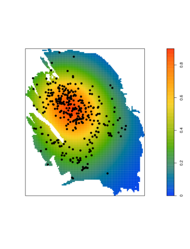
Figure 5: Projections on space of classic (left-most panel) and adaptive (right-most panel) kernel estimates of intensity (per square km) for the data in Figure 1. The pilot bandwidths are $h_{g,S}=9.4$ and $h_{g,T}=182.5$, whilst $h_{a,S}=6.9$ and $h_{a,T}=212.9$

The risk of using the same bandwidths $h_{S},h_{T}$ at all points of $\Psi$ is that, as all one-size-fits-all solutions, this approach tends to oversmooth in regions that are rich in points while at the same time it does not smooth enough in sparser regions. To overcome this drawback we propose to use an adaptive smoother as introduced for classic random variables by Abramson [1]. In a spatial context, such estimators were studied by Davies et al. [9] for Poisson point processes and in Van Lieshout [20] for general point processes with interaction between the points. The underlying idea is to weigh the bandwidth at $(s,t)\in\Psi$ by a scalar that is inversely proportional to $\sqrt{\lambda(s,t)}$. The power $1/2$ is motivated by asymptotics (cf. Abramson [1] and Van Lieshout [20]), in practice other powers could also be used.

Formally, set

$$\hat{\lambda}_{A}(x_{0};h_{S},h_{T})=\sum_{(s,t)\in\Psi\cap(W_{S}\times W_{T})}\frac{\kappa(H(c(s,t)h_{S},c(s,t)h_{T})^{-1}(x_{0}-(s,t)))}{w(((s,t),h_{S},h_{T})\,c(s,t)^{3}\,h_{S}^{2}\,h_{T}}$$ (1)

for $x_{0}\in W_{S}\times W_{T}$. Here $H(h_{1},h_{2})$, $h_{1},h_{2}>0$, is a $3\times 3$ diagonal matrix whose first two entries are $h_{1}$ and whose third entry is $h_{2}$,

$$c(s,t)=\left(\frac{\lambda(s,t)}{(\prod_{z\in\Psi\cap(W_{S}\times W_{T})}\lambda(z))^{1/N(\Psi\cap W_{S}\times W_{T})}}\right)^{-1/2},$$ (2)

$w((s,t),h_{S},h_{T})$ is an edge correction term and $\kappa$ is a symmetric probability density function, the kernel. Since $\lambda$ is unknown, $c(s,t)$ must be estimated. We will do so by plugging in a standard kernel estimator with fixed bandwidth.

To select the bandwidth, we propose the following completely non-parametric and computationally easy algorithm.

Algorithm 1.

Let $\psi$ be a non-empty spatio-temporal point pattern that is observed in the window $W_{S}\times W_{T}$. Then

1. Choose global bandwidth $h_{g,S}$, $h_{g,T}$ by minimising

   $$\left|\sum_{x\in\psi\cap(W_{S}\times W_{T})}\frac{1}{\hat{\lambda}(x;h_{S},h_{T})}-\ell(W_{S})\ell(W_{T})\right|$$ (3)

   over $h_{S},h_{T}>0$ (with minimal $h_{S}^{2}h_{T}$ in case of multiple solutions) where

   $$\hat{\lambda}(x;h_{S},h_{T})=\frac{1}{h_{S}^{2}h_{T}}\sum_{y\in\psi\cap(W_{S}\times W_{T})}\kappa\left(H(h_{S},h_{T})^{-1}(x-y)\right).$$

2. Calculate, for each $x\in\psi\cap(W_{S}\times W_{T})$, the edge-corrected pilot estimator

   $$\hat{\lambda}_{c}(x;h_{g,S},h_{g,T})=\frac{1}{h_{g,S}^{2}h_{g,T}}\sum_{y\in\psi\cap(W_{S}\times W_{T})}\frac{\kappa\left(H(h_{g,S},h_{g,T})^{-1}(x-y)\right)}{w(y,h_{g,S},h_{g,T})}$$

   with local edge correction weights

   $$w(y,h_{g,S},h_{g,T})=\frac{1}{h_{g,S}^{2}h_{g,T}}\int_{W_{S}\times W_{T}}\kappa\left(H(h_{g,S},h_{g,T})^{-1}(z-y)\right)dz.$$

3. Choose adaptive bandwidths $h_{a,S}$, $h_{a,T}$, by minimising

   $$\left|\sum_{x\in\psi\cap(W_{S}\times W_{T})}\frac{1}{\hat{\lambda}_{A}(x;h_{S},h_{T})}-\ell(W_{S})\,\ell(W_{T})\right|$$

   over $h_{S},h_{T}>0$ (with minimal $h_{S}^{2}h_{T}$ in case of multiple solutions) where $\hat{\lambda}_{A}$ is given by (1) and (2) with $w\equiv 1$ upon plugging in the edge-corrected pilot estimator $\hat{\lambda}_{c}$ for $\lambda$.

Local edge correction weights, as suggested by Van Lieshout [18], for the adaptive kernel estimator take the form

$$w(y,h_{a,S},h_{a,T})=\int_{W_{S}\times W_{T}}\frac{\kappa\left(H(\hat{c}(y)\,(h_{a,S},h_{a,T}))^{-1}(z-y)\right)}{h_{a,S}^{2}h_{a,T}(\hat{c}(y))^{3}}\,dz$$

and ensure that (1) is mass preserving in the sense that its integral over $W_{S}\times W_{T}$ is equal to the number of points in $\psi\cap(W_{S}\times W_{T})$. In selecting the bandwidth in steps 1 and 3 of Algorithm 1, no edge correction is applied in order to obtain a clear optimum (see Cronie and Van Lieshout [8]).

The justification of Algorithm 1 lies in the Campbell–Mecke theorem (cf. Chiu et al. [6]), which states that

$${\mathbb{E}}\left[\sum_{x\in\Psi\cap(W_{S}\times W_{T})}\frac{1}{\lambda(x)}\right]=\ell(W_{S})\ell(W_{T}).$$

The first step is a modification to space-time of the Cronie–Van Lieshout bandwidth selector [8] for purely spatial point processes. An important difference is that in space one optimises over a single parameter and usually, but not always, there is only one minimiser. In the space-time domain, the optimisation is done with respect to two parameters, $h_{S}$ and $h_{T}$. Therefore, as a rule, a curve of minimisers is found in steps 1 and 3 of Algorithm 1. We pick the optimiser having the smallest scale $h_{S}^{2}h_{T}$.

For our earthquake catalogue, the results are shown in Figures 5 and 6. The pilot bandwidths are $h_{g,S}=9.4$ and $h_{g,T}=182.5$. The corresponding edge-corrected projections on space and time are shown in, respectively, the left-most panel of Figure 5 and the broken line in Figure 6. They should be compared to the projections of the edge-corrected adaptive kernel estimate with $h_{a,S}=6.9$ and $h_{a,T}=212.9$ shown in the right-most panel in Figure 5 and the solid line in Figure 6. Note that $\hat{\lambda}_{A}$ attains higher values in the central reservoir than $\hat{\lambda}$, lower values near the eastern border of the gas field. From a temporal perspective, the extremes in years with a large number of earthquakes are somewhat more pronounced for the adaptive kernel estimate.

Figure 6: Expected number of earthquakes using classic (broken line) and adaptive (solid line) kernel estimates for the data in Figure 1 over $27$ equal time intervals. The pilot bandwidths are $h_{g,S}=9.4$ and $h_{g,T}=182.5$, whilst $h_{a,S}=6.9$ and $h_{a,T}=212.9$

3.2 Inhomogeneous spatio-temporal K- and J-functions

Having estimated the trend, we now turn our attention to the inter-point interactions. To quantify such interaction, information about the joint distributions of pairs, or tuples, of points is required, which is formalised by the higher-order analogues of the intensity function, the product densities $\lambda^{(n)}$. Heuristically, $\lambda^{(n)}((s_{1},t_{1}),\ldots,(s_{n},t_{n}))ds_{1}dt_{1}\cdots ds_{n}dt_{n}$ is the probability that $\Psi$ places points at each of the infinitesimal regions $ds_{i}dt_{i}$ around $(s_{i},t_{i})$, $i=1,\dots,n$.

A spatio-temporal point process $\Psi$ on ${\mathbb{R}}^{2}\times{\mathbb{R}}$ is said to be intensity-reweighted moment stationary (IRMS) (cf. Cronie and Van Lieshout [7]) if its product densities $\lambda^{(n)}$ of all orders exist, $\bar{\lambda}=\inf_{(s,t)}\lambda(s,t)>0$ and, for all $n\geq 1$, $\xi_{n}$ is translation invariant in the sense that

$$\xi_{n}((s_{1},t_{1})+(a,b),\ldots,(s_{n},t_{n})+(a,b))=\xi_{n}((s_{1},t_{1}),\ldots,(s_{n},t_{n}))$$

for almost all $(s_{1},t_{1}),\ldots,(s_{n},t_{n})\in{\mathbb{R}}^{2}\times{\mathbb{R}}$ and all $(a,b)\in{\mathbb{R}}^{2}\times{\mathbb{R}}$. Here $\xi_{n}$ are the $n$-point correlation functions defined in terms of the $\lambda^{(n)}$ by setting $\xi_{1}\equiv 1$ and for other $n$ recursively by

$$\frac{\lambda^{(n)}((s_{1},t_{1}),\ldots,(s_{n},t_{n}))}{\prod_{k=1}^{n}\lambda(s_{k},t_{k})} =\sum_{k=1}^{n}\sum_{D_{1},\ldots,D_{k}}\prod_{j=1}^{k}\xi_{|D_{j}|}((s_{i},t_{i}):i\in D_{j}),$$ (4)

where $\sum_{D_{1},\ldots,D_{k}}$ is a sum over all possible $k$-sized partitions $\{D_{1},\ldots,D_{k}\}$, $D_{j}\neq\emptyset$, of the set $\{1,\ldots,n\}$ and $|D_{j}|$ denotes the cardinality of $D_{j}$. For a Poisson point process, in which there are no correlations between the points, $\xi_{n}\equiv 0$ for $n\geq 1$. The point process is said to be second order intensity-reweighted stationary (SOIRS) if the translation invariance holds up to $n=2$ (see Gabriel and Diggle [13]).

Various summary statistics exist to explore inter-point interactions. Write

$$S_{h_{S}}^{h_{T}}=\{(s,t)\in{\mathbb{R}}^{2}\times{\mathbb{R}}:\|s\|\leq h_{S},|t|\leq h_{T}\}$$

and let $\Psi$ be an IRMS spatio-temporal point process. Then the statistic

$$J_{n}(h_{S},h_{T})=\int_{S_{h_{S}}^{h_{T}}}\cdots\int_{S_{h_{S}}^{h_{T}}}\xi_{n+1}((0,0),(s_{1},t_{1}),\ldots,(s_{n},t_{n}))\prod_{i=1}^{n}ds_{i}dt_{i}$$

quantifies cumulative correlations of order $n=1,2,\dots$ up to ranges $h_{S}\geq 0$ in space and $h_{T}\geq 0$ in time. Multiple orders can be combined. For example, Van Lieshout [17] proposed

$$J_{\rm inhom}(h_{S},h_{T})=1+\sum_{n=1}^{\infty}\frac{(-\bar{\lambda})^{n}}{n!}J_{n}(h_{S},h_{T})$$ (5)

for all spatial ranges $h_{S}\geq 0$ and temporal ranges $h_{T}\geq 0$ for which the series is absolutely convergent. Values greater than one are indicative of repulsion, values smaller than one suggest clustering. For further details, the reader is referred to Cronie and Van Lieshout [7]. Truncating at $n=2$,

$$J_{\rm inhom}(h_{S},h_{T})-1\approx-\bar{\lambda}\left(K_{\rm inhom}(h_{S},h_{T})-\ell(S_{h_{S}}^{h_{T}})\right)$$

in terms of the inhomogeneous $K$-function

$$K_{\rm inhom}(h_{S},h_{T})=\int_{S_{h_{S}}^{h_{T}}}\left[\xi_{2}((0,0),(s_{1},t_{1}))+1\right]ds_{1}dt_{1}$$

of Gabriel and Diggle [13], which is well-defined under the SOIRS assumption. Values greater or smaller than the volume of $S_{h_{S}}^{h_{T}}$ are indicative of, respectively, clustering and inhibition between points.

Figure 7: Graphs of $(\hat{K}_{\rm{inhom}}(r,100r)/(2\pi))^{1/3}$ against $r$ (solid line, left-most panel), of $\hat{G}(1-u^{y}_{r,100r})$ (solid line, right-most panel) and $G^{!y}(1-u^{y}_{r,100r})$ (broken line, right-most panel) for the data in Figure 1. The units are km in space and days in time.

In practice, one must estimate these statistics based on a pattern observed in $W_{S}\times W_{T}$. The definition of the inhomogeneous $J$-function does not immediately suggest a suitable estimator. However, Cronie and Van Lieshout [7] showed that, for all $y\in{\mathbb{R}}^{2}\times{\mathbb{R}}$,

$$J_{\rm inhom}(h_{S},h_{T})=\frac{G^{!y}(1-u_{h_{S},h_{T}}^{y})}{G(1-u_{h_{S},h_{T}}^{y})}$$ (6)

whenever well-defined and the denominator is greater than zero. Here the function $u_{h_{S},h_{T}}^{y}$ is defined by

$$u_{h_{S},h_{T}}^{y}(s,t)=\frac{\bar{\lambda}1\{\|a-s\|\leq h_{S},|b-t|\leq h_{T}\}}{\lambda(s,t)},\quad y=(a,b)\in{\mathbb{R}}^{2}\times{\mathbb{R}},$$

and $G$ is the generating functional of $\Psi$, that is,

$$G(1-u_{h_{S},h_{T}}^{y})={\mathbb{E}}\left[\prod_{(s,t)\in\Psi}\left(1-\frac{\bar{\lambda}1\{\|a-s\|\leq h_{S},|b-t|\leq h_{T}\}}{\lambda(s,t)}\right)\right]$$

for $h_{S},h_{T}\geq 0$, under the convention that empty products take the value one. $G^{!y}$ is defined similarly in terms of the distribution of $\Psi\setminus\{y\}$ given there is a point of $\Psi$ at $y$. Being expectations, the numerator and denominator in equation (6) can be estimated in a straightforward manner. Write $W_{S}^{\ominus{h_{S}}}$ for the set of points in $W_{S}$ that are at least $h_{S}$ away from the border of $W_{S}$ and let $W_{T}^{\ominus h_{T}}$ be the similarly eroded temporal domain. Then, given a finite point grid $L\subseteq W_{S}\times W_{T}$,

$$\frac{1}{N(L\cap(W_{S}^{\ominus h_{S}}\times W_{T}^{\ominus h_{T}}))}\sum_{l\in L\cap(W_{S}^{\ominus h_{S}}\times W_{T}^{\ominus h_{T}})}\left[\prod_{x\in\Psi\cap(l+S_{h_{S}}^{h_{T}})}\left(1-\frac{\bar{\lambda}}{\lambda(x)}\right)\right]$$

is an unbiased estimator of the denominator in (6). An unbiased estimator for the numerator is obtained analogously. Finally,

$$\hat{K}_{\rm{inhom}}(h_{S},h_{T})=\frac{1}{\ell(W_{S}^{\ominus h_{S}})\ell(W_{T}^{\ominus h_{T}})}\sum_{x\in\Psi\cap(W_{S}^{\ominus h_{S}}\times W_{T}^{\ominus h_{T}})}\mathop{\sum\nolimits^{\neq}}_{y\in\Psi\cap(x+S_{h_{S}}^{h_{T}})}\frac{1}{\lambda(x)\lambda(y)}$$

is an unbiased estimator of $K_{\rm{inhom}}(h_{S},h_{T})$. Note that the intensity functions are unknown. A practical solution is to plug in their estimated counterparts (cf. Section 3.1).

For the earthquake catalogue depicted in Figure 1, consider Figure 7. The solid line in the left-most panel of the figure is the graph of $(\hat{K}_{\rm{inhom}}(r,100r)/(2\pi))^{1/3}$ for the earthquake data. It lies above the graph of the same function for a Poisson point process (shown as a broken line in the left-most panel of the figure), suggesting attraction between the points. In the right-most panel of Figure 7, the graph of $\hat{G}(1-u^{y}_{r,100r})$ estimated from the data lies above that of $G^{!y}(1-u^{y}_{r,100r})$, which confirms the suggested clustering.

4 Explanatory variables

Gas production and pore pressure (cf. Section 2.4 and 2.5) may well have an effect on the earthquake rates. However, they are measured only for a limited number of locations and times. Therefore, in this session, we discuss how to calculate appropriate values for the entire space-time domain.

4.1 Non-parametric smoothing of gas production values

Monthly production values are available for the $29$ production wells shown by a cross in Figure 2 over the time period 1956–2021. The gas extracted from the Eemskanaal-13 bore hole is listed separately from the other ones at the Eemskanaal site. The reason is that the Eemskanaal-13 pipe is not drilled vertically but bends underground in such a way that it is depleting the Harkstede block (cf. Section 2.5). Therefore we assign its production to the location of the observation well at Harkstede. Thus, we end up with a spatial pattern of $30$ points, the locations of the $29$ production wells as well as the Harkstede proxy for the Eemskanaal-13 pipe.

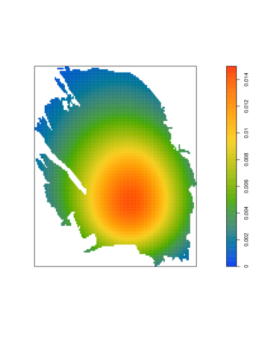
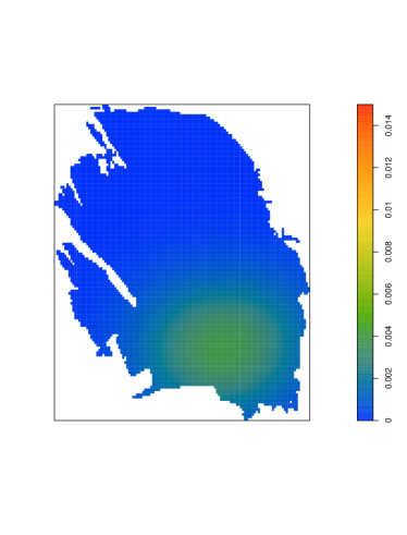
Figure 8: Smoothed monthly gas production over January 2012 (left-most panel) and January 2021 (right-most panel) in Nbcm per square kilometre.

In order to smooth the production out in a mass-preserving fashion, an adaptive kernel method similar to that proposed in Section 3 for the intensity function can be used. More specifically, write $V(s,t)\geq 0$ for the volume of gas produced at a well at $s$ in month $t$ and write $\phi$ for the well pattern. We then use the spatial counterpart of Algorithm 1 proposed by Van Lieshout [20] to select bandwidths $h_{g,S}$ and $h_{a,S}$ and set, for $s_{0}\in W_{S}$, $t_{0}\in W_{T}$,

$$\hat{\lambda}_{V}((s_{0},t_{0}),\phi)=\sum_{(s,t)\in\phi}\frac{V(s,t)1\{t_{0}\in m(t)\}}{w(s,h_{a,S})h_{a,S}^{2}\hat{c}(s;h_{g,S})^{2}\ell(m(t))}\kappa\left(\frac{s_{0}-s}{h_{a,S}\hat{c}(s;h_{g,S})}\right)$$

based on spatial kernel $\kappa$ and using local edge correction weights $w$, cf. Section 3. In time, $V(s,t)$ is spread evenly over the $\ell(m(t))$ days in the month $m(t)$ to which $t\in W_{T}$ belongs. This smoother is mass preserving, as

$$\int_{W_{S}\times W_{T}}\hat{\lambda}_{V}((s,t_{i}),\phi)ds = \sum_{(s,t)\in\phi}\frac{V(s,t)}{w(s,h_{a,S})}\int_{W_{S}}\frac{1}{h_{a,S}^{2}\hat{c}(s;h_{g,S})^{2}}\kappa\left(\frac{s_{0}-s}{h_{a,S}\hat{c}(s;h_{g,S})}\right)ds_{0}$$

$$= \sum_{(s,t)\in\phi}V(s,t).$$

For the data discussed in Section 2.4, Algorithm 1 yields a pilot bandwidth $h_{g,S}=7.6$ and $h_{a,S}=6.9$. The resulting gas production maps for January 2012, before legislation to phase out gas extraction came into effect, and for January 2021 are shown in Figure 8. The decrease in extracted volume is evident. Moreover, the remaining production is located mostly in the southern part of the gas field.

4.2 Regression analysis for pore pressure

From Figure 4, it is clear that the pore pressure in the reservoir is decreasing in time. The trend is similar for most wells, with some exceptions, for example because of large faults or at the periphery of the field. Recall from Section 2 that our earthquake catalogue contains tremors from January 1st, 1995 onward. If we wish to use the pore pressure as an explanatory variable in a monitoring model, we need their values over the same time period. Thus, our goal in this section is to perform a regression analysis using only the $352$ pore pressure measurements from January 1st, 1995, and later.

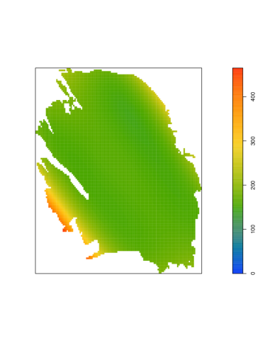
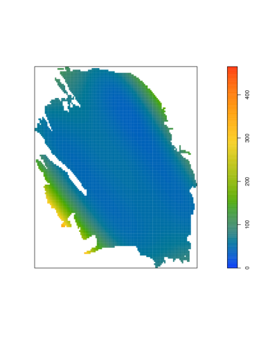
Figure 9: Estimated pore pressure maps at midnight on January 1st in the years 1995 (left-most panel) and 2022 (right-most panel) in bara.

Suppose that the observed pore pressures can be seen as realisations of stochastic variables $X(s,t)$ that can be decomposed in a trend term $m((s,t);\beta)$ and noise $E(s,t)$ as follows:

$$X(s,t)=m((s,t);\beta)+E(s,t).$$

We assume that the $E(s,t)$ are independent and normally distributed with mean zero and variance $\sigma^{2}$. For the trend fit a polynomial in space and time,

$$m((s,t);\beta) = \beta_{1}+\beta_{2}t+\beta_{3}t^{2}+\beta_{4}(s-s_{0})_{1}+\beta_{5}(s-s_{0})_{2}+\beta_{6}(s-s_{0})_{1}^{2}$$

$$+ \beta_{7}(s-s_{0})_{1}(s-s_{0})_{2}+\beta_{8}(s-s_{0})_{2}^{2}+\beta_{9}(s-s_{0})_{1}^{3}$$

$$+ \beta_{10}(s-s_{0})_{1}^{2}(s-s_{0})_{2}+\beta_{11}(s-s_{0})_{1}(s-s_{0})_{2}^{2}+\beta_{12}(s-s_{0})_{2}^{3}$$

$$+ \beta_{13}(s-s_{0})_{1}^{4}+\beta_{14}(s-s_{0})_{1}^{3}(s-s_{0})_{2}+\beta_{15}(s-s_{0})_{1}^{2}(s-s_{0})_{2}^{2}$$

$$+ \beta_{16}(s-s_{0})_{1}(s-s_{0})_{2}^{3}+\beta_{17}(s-s_{0})_{2}^{4}+\beta_{18}t(s-s_{0})_{1}+\beta_{19}t(s-s_{0})_{2}$$

$$+ \beta_{20}t(s-s_{0})_{1}^{2}+\beta_{21}t(s-s_{0})_{1}(s-s_{0})_{2}+\beta_{22}t(s-s_{0})_{2}^{2}+\beta_{23}t(s-s_{0})_{1}^{3}$$

$$+ \beta_{24}t(s-s_{0})_{1}^{2}(s-s_{0})_{2}+\beta_{25}t(s-s_{0})_{1}(s-s_{0})_{2}^{2}+\beta_{26}t(s-s_{0})_{2}^{3}$$

where we centre the spatial locations at $s_{0}=(750,5900)$ in the UTM system (zone $31$ in units of km) and take days as the temporal unit counting from January 1st, 1995. The parameter $\beta=(\beta_{1},\dots,\beta_{26})$ can be estimated by the least squares method.

The fitted pore pressure maps at midnight January 1st in the years 1995 and 2022 are given in Figure 9. One may note the elevated values in the Harkstede block in the South-West as well as those in the Northern border regions.

Figure 10: Observed pore pressure values against fitted values (left-most panel) and the histogram of residuals (right-most panel).

To validate the model, the actual pore pressure measurements are plotted against their fitted values in the left-most panel of Figure 10. The graph seems reasonably close to a straight line. The histogram of the residuals is shown in the right-most panel of Figure 10. Most residuals are quite small and the histogram is centred around zero with estimated standard deviation $\hat{\sigma}=7.17$ bara.

5 Discussion and further work

In this paper, we carried out an exhaustive second order exploratory analysis of the spatio-temporal point pattern of earthquakes recorded in the Groningen gas field since January 1995. To do so, we needed to develop new methodology. We proposed an adaptive kernel smoothing technique for estimating the intensity function and suggested a practical algorithm for selecting the spatial and temporal bandwidths. The estimated intensity function was then plugged into state of the art inhomogeneous summary statistics to quantify the degree of clustering in the earthquake catalogue. We also applied our new adaptive kernel smoothing technique to monthly gas production figures. Finally, we performed a regression analysis on pore pressure data for the gas field.

In the rate-and-state models (e.g. Candela et al. [4], Dempsey and Suckale [10] and Richter et al. [24]) that can be seen as the state of the art in modelling the seismic hazard and that is being used for planning, the earthquake intensity $\lambda$ (the rate) is assumed to be inversely proportional to a state variable $\Gamma$, that is,

$$\lambda(s,t)\propto\Gamma(s,t)^{-1},\quad(s,t)\in W_{S}\times W_{T}.$$

The state variable $\Gamma(s,t)$ is defined by the ordinary differential equation

$$d\Gamma(s,t)=\alpha\left[dt-\Gamma(s,t)dS(s,t)\right],$$

where $S$ is the Coulomb stress with a reduced friction coefficient and $\alpha>0$. According to Richter et al. [24], Coulomb stress changes are proportional to changes in pore pressure $X(s,t)$, that is $dS(s,t)=-\beta dX(s,t)$ for some scalar $\beta>0$. Consequently, the differential equation for the state can be written as

$$d\Gamma(s,t)=\alpha\left[dt+\beta\Gamma(s,t)dX(s,t)\right].$$

Multiplying both sides by $\exp(-\alpha\beta X(s,t))$, it follows that

$$\frac{d}{dt}\left[\Gamma(s,t)e^{-\alpha\beta X(s,t)}\right]=\alpha e^{-\alpha\beta X(s,t)}.$$ (7)

The Euler discretisation reads

$$\Gamma(s,t+\Delta)=\left(\Gamma(s,t)+\Delta\alpha\right)\exp\left[\alpha\beta(X(s,t+\Delta)-X(s,t))\right],\quad s\in W_{S},$$

upon discretising $W_{T}$ in time steps of length $\Delta$.

In the rate-and-state model, the earthquakes constitute a Poisson point process with intensity function $\lambda$, possibly modified by a fault map. The parameters $\alpha$ and $\beta$ and the initial state $\Gamma(s,0)\equiv 1/\lambda_{0}$ are treated as unknowns and can be estimated, for example by the maximum likelihood method.

Based on the exploratory analysis in Sections 3 and 4, the rate-and-state model can be criticised on several points. As we saw in Section 3, the earthquake pattern exhibits clustering. Since by definition the points in any Poisson point process do not interact with one another, the apparent clustering of earthquakes cannot be described by the rate-and-state model. Secondly, the pressure values are assumed to be known everywhere, in practice by interpolation of the measurements. Proceeding in this way, the uncertainty in the interpolations is ignored. It would be better to treat the $X(s,t)$ as a random field. Lastly, the varying gas extraction is not taken into account.

Based on the above considerations, we propose the following model. Set $\Gamma(s,0)=1/\lambda_{0}$ and iterate

$$\Gamma(s,t+\Delta)=\left(\Gamma(s,t)+\alpha\Delta\right)\exp\left[\alpha\beta(m(s,t+\Delta)-m(s,t))\right]\exp\left[\alpha\beta(E(s,t+\Delta)-E(s,t))\right]$$

where $m$ and $E$ are as in Section 4.2. The gas production and random effects, if any, may be included in the following way. Let $\Psi$ be a Cox process (cf. Chiu et al. [6]) on $W_{S}\times W_{T}$ with driving random measure

$$\Lambda(s,t)=\frac{\exp\left[\theta_{1}+\theta_{2}\tilde{V}(s,t)+U(s,t)\right]}{\Gamma(s,t)}$$

where $\tilde{V}(s,t)$ is the gas extracted at $s$ during the year preceeding time $t$ and $U(s,t)$ is a correlated Gaussian field that accounts for random effects. Monitoring can then be based on the posterior distribution of $\Lambda$ or, equivalently $\Gamma$ and $U$, given the recorded earthquakes. The implementation requires careful use of Markov chain Monte Carlo techniques and is the topic of our ongoing research.

References

- [1] Abramson, I.S. (1982). On bandwidth variation in kernel estimates – A square root law. The Annals of Statistics 10:1217–1223.
- [2] Baki, Z., Lieshout, M.N.M. van (2022). The influence of gas production on seismicity in the Groningen field. Proceedings of the 10th International Workshop on Spatio-Temporal Modelling METMA X, pp. 163–167.
- [3] Bourne, S.J., Oates, S.J., Van Elk, J. (2018). The exponential rise of induced seismicity with increasing stress levels in the Groningen gas field and its implications for controlling seismic risk. Geophysicial Journal International 213:1693–1700.
- [4] Candela, T. et al. (2019). Depletion-induced seismicity at the Groningen gas field: Coulomb rate-and-state models including differential compaction effect. Journal of Geophysical Research: Solid Earth 124:7081–7104.
- [5] Chacón, J.E., Duong, T. (2018). Multivariate Kernel Smoothing and its Applications. CRC Press.
- [6] Chiu, S.N., Stoyan, D., Kendall, W.S., Mecke, J. (2013). Stochastic Geometry and its Applications. Wiley, 3rd ed.
- [7] Cronie, O., Lieshout, M.N.M. van (2015). A -function for inhomogeneous spatio-temporal point processes. Scandinavian Journal of Statistics 42:562–579.
- [8] Cronie, O., Lieshout, M.N.M. van (2018). A non-model based approach to bandwidth selection for kernel estimators of spatial intensity functions. Biometrika 105:455–462.
- [9] Davies, T.M., Flynn, C.R., Hazelton, M.L. (2018). On the utility of asymptotic bandwidth selectors for spatially adaptive kernel density estimation. Statistics and Probabability Letters 138:75–81.
- [10] Dempsey, D., Suckale, J. (2017). Physics-based forecasting of induced seismicity at Groningen gas field, the Netherlands. Geophysical Research Letters 22:7773–7782.
- [11] Diggle, P. (1985). A kernel method for smoothing point process data. Applied Statistics 34:138–147.
- [12] Dost, B., Goutbeek, F., Van Eck, T., Kraaijpoel, D. (2012). Monitoring induced seismicity in the North of the Netherlands: Status report 2010. Scientific Report KNMI WR 2012–03.
- [13] Gabriel, E., Diggle, P. J. (2009). Second-order analysis of inhomogeneous spatio-temporal point process data. Statistica Neerlandica 63:43–51
- [14] Geerdink, E. (2014). Modeling the induced earthquakes in Groningen as a Poisson process using GLM and GAM. BSc thesis, University of Groningen
- [15] Hettema, M.H.H., Jaarsma, B., Schroot, B.M., Van Yperen, G.C.N. (2017). An empirical relationship for the seismic activity rate of the Groningen gas field. Netherlands Journal of Geosciences 96:149–161.
- [16] Hove, E. van, Van Lingen, R., Riemens, S. (2015). Geïnduceerde aardbevingen in gasveld Groningen. Een statistische analyse. BSc thesis, University of Twente.
- [17] Lieshout, M. N. M. van (2011). A -function for inhomogeneous point processes. Statistica Neerlandica 65:183–201
- [18] Lieshout, M.N.M. van (2012). On estimation of the intensity function of a point process. Methodology and Computing in Applied Probability 14:567–578.
- [19] Lieshout, M.N.M. van (2020). Infill asymptotics and bandwidth selection for kernel estimators of spatial intensity functions. Methodology and Computing in Applied Probability 22:995–1008.
- [20] Lieshout, M.N.M.van (2021). Infill asymptotics for adaptive kernel estimators of spatial intensity. Australian and New Zealand Journal of Statistics 63:159–181, 2021.
- [21] Lo, P.H. (2017). An iterative plug-in algorithm for optimal bandwidth selection in kernel intensity estimation for spatial data. PhD Thesis, Technical University of Kaiserslautern.
- [22] Ogata, Y. (1988). Statistical models for earthquake occurrences and residual analysis for point processes. Journal of the American Statistical Association 83-401:9–27.
- [23] Post, R.A.J. et al. (2021). Interevent-time distribution and aftershock frequency in non-stationary induced seismicity. Scientific Reports 11, 3540.
- [24] Richter, G., Hainzl, S., Dahm, T., Zőller, G. (2020). Stress-based statistical modeling of the induced seismicity at the Groningen gas field, The Netherlands. Environmental Earth Sciences 79, 252.
- [25] Sijacic, D., Pijpers, F., Nepveu, M., Van Thienen–Visser, K. (2017). Statistical evidence on the effect of production changes on induced seismicity. Netherlands Journal of Geosciences 96:27–38.
- [26] Trampert J., Benzi R., Toschi F. (2022). Implications of the statistics of seismicity recorded within the Groningen gas field. Netherlands Journal of Geosciences 101, to appear.
- [27] Vlek, C. (2019). Rise and reduction of induced earthquakes in the Groningen gas field, 1991–2018: Statistical trends, social impacts, and policy change. Environmental Earth Sciences 78:1–14.