Advancing Reacting Flow Simulations
with Data-Driven Models

The use of machine learning algorithms to predict behaviors of complex systems is booming. However, the key to an effective use of machine learning tools in multi-physics problems, including combustion, is to couple them to physical and computer models. The performance of these tools is enhanced if all the prior knowledge and the physical constraints are embodied. In other words, the scientific method must be adapted to bring machine learning into the picture, and make the best use of the massive amount of data we have produced, thanks to the advances in numerical computing. The present chapter reviews some of the open opportunities for the application of data-driven reduced-order modeling of combustion systems. Examples of feature extraction in turbulent combustion data, empirical low-dimensional manifold (ELDM) identification, classification, regression, and reduced-order modeling are provided.

1 Introduction

The simulation of turbulent combustion is a very challenging task for a number of aspects beyond turbulence. Combustion is intrinsically multi-scale and multi-physics. It is characterized by a variety of scales inherently coupled in space and time through thermo-chemical and fluid dynamic interactions [1]. Typical chemical mechanisms describing the evolution of fuels consist of hundreds of species involved in thousands of reactions, spanning 12 orders of magnitude of temporal scales [2]. The interaction of these scales with the fluid dynamic ones defines the nature of the combustion regime as well as the limiting process in determining the overall fuel oxidation rate [3]. When the characteristic chemical scales are much smaller than the fluid dynamic ones, the combustion problem becomes a mixing one (i.e., mixed is burnt [4]): combustion and chemistry are decoupled, and the problem is highly simplified. Likewise, for chemical timescales much larger than the fluid dynamic ones, the system can be described taking into account chemistry only, neglecting the role of fluid dynamics altogether.

The intensity of interactions between turbulent mixing and chemistry is measured using the Damköhler number, defined as the ratio between the characteristic mixing, $\tau_{m}$, and chemical, $\tau_{c}$, timescales:

$$Da=\frac{\tau_{m}}{\tau_{c}}.$$ (1)

In terms of the Damköhler number, $Da\gg 1$ indicates a mixing-controlled, fast chemistry process. On the other hand, $Da\ll 1$ denotes a chemistry-controlled, slow chemistry process. Most practical combustion systems operate at conditions characterized by a non-negligible overlap between flow and chemical scales. This is particularly true for novel combustion technologies, where the use of diluted conditions and the enhanced mixing leads to a $Da$ distribution close to unity. This grants some control on the combustion process, thanks to the increase of the characteristic chemical scales compared to the mixing ones. In particular, the operating conditions (temperature and compositions) can be adjusted in such a way that the emissions are kept below the required values [5], [6], [7]. The condition $Da\approx 1$ is generally referred to as finite-rate chemistry, to indicate that combustion is not infinitely fast but of finite speed.

Modeling finite-rate combustion regimes is very challenging because both fluid mechanics and chemistry effects must be accounted for accurately. In particular, chemistry cannot be described using simplified global mechanisms, and this results in a significant computational burden of combustion simulations. The resolution of turbulent combustion problems requires the resolution of hundreds of transport equations for (tightly coupled) chemical species on top of the conservation equations for mass, momentum, and energy. Beside the high dimensionality of the problem [8], the transport equations of reacting scalars require closure models, when the reacting structures are not fully resolved on the numerical grid.

The challenges associated with turbulent combustion modeling make the use of machine learning very attractive. While turbulent combustion models are spread across combustion industries, their current predictive capabilities fall well short of what would be needed in decision making for new design and regulation [1]. High-fidelity, direct numerical simulations (DNS) of combustion systems are still limited to isolated aspects of a turbulent combustion process and simple building blocks. Still, these high-fidelity simulations are rich in information that could help decode the complexity of turbulence-chemistry interactions and guide the development of filtered and lower-fidelity modeling approaches for faster evaluations.

The objective of the present chapter is to demonstrate the potential of data-driven modeling in the context of combustion simulations. In particular, we present:

• The application of principal component analysis (PCA) and other linear and nonlinear techniques to identify low-dimensional manifolds in high-fidelity combustion data-sets, and to reveal the key features of complex non-equilibrium phenomena. Different techniques are compared to PCA, including non-negative matrix factorization (NMF), autoencoders, and local PCA in §3.

• The development of reduced-order models (ROMs), to be used in conjunction with, or to replace high-fidelity simulation tools, to reduce the burden associated with the large number of species in detailed chemical mechanisms. First, the use of transport models based on PCA is presented in §4. Finally, the application of the data-driven adaptive-chemistry approach based on the combination of classification and chemical mechanism reduction is discussed in §5.

2 Combustion Data Sets

The structure of combustion data sets differs from the one seen in pure fluid mechanics applications (presented in Chapter 4). The data set encountered in multi-component reactive flows is stored in the form of a matrix $\mathbf{X}\in\mathbb{R}^{N\times Q}$. Each column of $\mathbf{X}$ is tied to one of the $Q$ thermo-chemical state-space variables: temperature $T$, pressure $p$, and $N_{s}-1$ chemical species mass (or mole) fractions, denoted $Y_{i}$ for the $i$th species. For open flames and atmospheric burners the pressure variable can be omitted. Each of the $N$ rows of $\mathbf{X}$ contains observations of all $Q$ variables at a particular point in the physical space and/or time (and sometimes, a point in the space of other independent parameters, as will be briefly discussed later). This structure of the data matrix is presented below:

$$\mathbf{X}=\begin{bmatrix}\vdots&\vdots&\vdots&\vdots&&\vdots\\ T&p&Y_{1}&Y_{2}&\dots&Y_{N_{s}-1}\\ \vdots&\vdots&\vdots&\vdots&&\vdots\\ \end{bmatrix}.$$ (2)

For such data set, $Q=N_{s}+1$. We will denote the $i$th row (observation) in $\mathbf{X}$ as $\mathbf{x}_{i}\in\mathbb{R}^{Q}$ and the $j$th column (variable) in $\mathbf{X}$ as $\mathbf{X}_{j}\in\mathbb{R}^{N}$. When the data set is only resolved in space and not resolved in time, $N$ represents the number of points on a spatial grid, and $\mathbf{X}$ can be thought of as a data snapshot (a notion much like the one discussed in Chapter 4). Typically, we can expect $N\gg Q$, however the magnitude of $Q$ will strongly depend on the number of species, $N_{s}$, involved in the chemical reactions and can even reach the order of thousands for more complex fuels [8].

Combustion data sets can be obtained from numerical solutions of combustion models, or from experimental measurements of laboratory flames. When generating a numerical data set, we incorporate information about the chemistry of the process by selecting a chemical mechanism for combustion of a given fuel. The mechanism determines which chemical species are involved in the specified chemical reactions, and it can vary in complexity.

For the discussion of data sets, it is useful to introduce the distinction between premixed and non-premixed combustion. In the premixed case, fuel and oxidizer are first mixed before they are burned. In the non-premixed combustion, fuel and oxidizer originate from separate streams and have to first mix for the combustion to occur. In this latter case, the mixture fraction variable is an important scalar quantity that specifies the local fuel to oxidizer ratio and is defined as:

$$Z=\frac{\nu Y_{F}-Y_{O_{2}}+Y_{O_{2},2}}{\nu Y_{F,1}+Y_{O_{2},2}},$$ (3)

for any point in space, where $Y_{F}$ is the local mass fraction of fuel, $Y_{O_{2}}$ is the local mass fraction of oxidizer in the mixture, and $\nu$ is their stoichiometric ratio [9]. $Y_{F,1}$ is the mass fraction of fuel in the fuel stream and $Y_{O_{2},2}$ is the mass fraction of oxidizer in the oxidizer stream. The complete combustion of fuel happens at the stoichiometric mixture fraction $Z_{st}$. If $Z<Z_{st}$, the mixture is called lean (fuel deficient) and if $Z>Z_{st}$, the mixture is called fuel rich.

Figure 1 presents an overview of frequently encountered numerical data sets, ordered schematically by the amount of information about the combustion process they contain. In particular:

• The zero-dimensional (0D) reactor model (e.g. perfectly stirred reactor (PSR)) assumes that combustion happens in a single point in space. This model can thus only include information about chemistry and thermodynamics of the combustion process evolving in time. It carries no information about spatial gradients of the thermo-chemical variables. The 0D reactor describes an ideal mixing process with $Da\ll 1$. When the data set is formed from the 0D reactor simulation, the $N$ rows of $\mathbf{X}$ are linked to points in time only.

• The steady laminar flamelet (SLF) model [10] assumes that fuel and oxidizer are two impinging streams, originating from the fuel and the oxidizer feed respectively. Combustion happens in infinitely thin sheets (flamelets) where fuel and oxidizer meet at varying stoichiometric proportions. The stoichiometry is specified by the mixture fraction variable, $Z$, and the thermo-chemical variables vary along the axis between pure oxidizer ($Z=0$) and pure fuel ($Z=1$). By varying the distance between the feeds (or the outlet velocities), a strain (specified by the strain rate $\chi$) is imposed on the flamelet, which can displace it from its equilibrium. The SLF model describes a non-premixed system with $Da\gg 1$. This is thus a two-parameter model with each row of $\mathbf{X}$ linked to one pair $(Z,\chi)$.

• The counterflow diffusion flame (CFDF) model [11] is similar to the SLF model, as it assumes two separate streams of fuel and oxidizer diffusing into one another (non-premixed system). However, in contrast to SLF, the flow equations for CFDF are solved in the physical space. Flow is parameterized by the velocity gradient parameter $a$, which is an equivalent of the local strain rate. In the CFDF, each row of $\mathbf{X}$ is linked to a point in the physical space and time.

• The one-dimensional turbulence (ODT) model [12], [13] can additionally incorporate the effects of turbulence by introducing eddy events on a one-dimensional domain. It allows for both spatial and temporal evolution of the flow. ODT can be used as a standalone model but can also serve as a subgrid model in large eddy simulations (LES).

• The Reynolds-averaged Navier-Stokes (RANS) models [14] solve the time-averaged equations describing fluid dynamics and hence any sources of unsteadiness coming from turbulence are averaged.

• The large eddy simulation (LES) [14] resolves large scales associated with the fluid dynamics processes but a subgrid model is required to account for processes occurring at the smallest scales. The choice for the subgrid model becomes particularly important in reactive flows, since combustion is inherently tied to the smallest scales.

• The direct numerical simulation (DNS) [14] allows for the most accurate description of the coupled interaction between fluid dynamics and the thermo-chemistry since all subgrid processes are resolved directly. The scarcity of the DNS data sets is due to the large computational cost of performing DNS simulations, especially for more complex fuels.

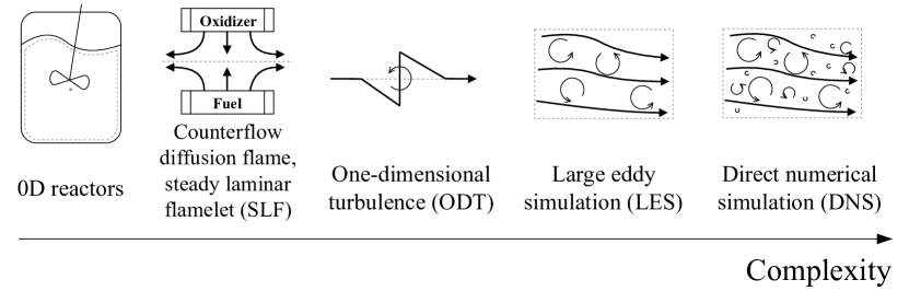
Figure 1: Examples of common numerical combustion data sets schematically presented on the axis of increasing complexity.

More information on combustion theory and combustion models can be found in [11], [15], or [16].

The selected data set is the starting point for applying a data science technique, and we often refer to those data sets as the training data. From the description of various data sets presented above, it is visible that the choice of the data set will be pertinent to the type and quality of the analysis performed. For instance, we can expect that features identified will depend on the amount of information about the coupled phenomena of turbulence and chemistry that was initially captured in the data set.

2.1 Data Preprocessing

Combustion data sets typically contain variables of different numerical ranges (e.g. both temperature, which can range from hundreds up to thousands, and mass (or mole) fractions of chemical species, which take values in the range $Y_{i}\in\langle 0,1\rangle$). Scaling the data set is crucial in order to balance the importance of all state-space variables [17]. The data set $\mathbf{X}$ can be centered and scaled as follows:

$$\widetilde{\mathbf{X}}=(\mathbf{X}-\mathbf{\bar{X}})\mathbf{D}^{-1},$$ (4)

where $\mathbf{\bar{X}}$ contains the mean observations of each variable. $\mathbf{D}$ is the diagonal matrix of scales, where the $j$th element, $d_{j}$, from the diagonal is the scaling factor corresponding to the $j$th state-space variable, $\mathbf{X}_{j}$. A few of the common scaling criteria are collected in Table 1. The result is a centered and scaled data matrix, $\widetilde{\mathbf{X}}$. Other preprocessing means can include outlier detection or data sampling. For the remainder of this chapter, we will assume that $\widetilde{\mathbf{X}}$ represents the matrix that has been adequately preprocessed.

Table 1: A few selected common data scaling criteria. $\sigma_{j}$ is the standard deviation, $max(\mathbf{X}_{j})$ is the maximum value, $min(\mathbf{X}_{j})$ is the minimum value, and $\bar{\mathbf{X}}_{j}$ is the mean observation of the $j$th state-space variable $\mathbf{X}_{j}$.

Scaling technique	Scaling factor, $d_{j}$
Auto	$\sigma_{j}$
Pareto	$\sqrt{\sigma_{j}}$
Range	$max(\mathbf{X}_{j})-min(\mathbf{X}_{j})$
VAST	$\sigma_{j}^{2}/\bar{\mathbf{X}}_{j}$

3 Feature Extraction Using Dimensionality Reduction Techniques

Dimensionality reduction techniques offer a way to represent high-dimensional combustion data sets in a new, lower-dimensional basis. Such data representations are referred to as low-dimensional manifolds. Techniques such as PCA, NMF or autoencoders can extract those manifolds in an empirical way from the training data sets. This approach belongs to the family of empirical low-dimensional manifolds (ELDMs) [1], [18], and it is based on the idea that compositions occurring in combustion systems lie close to a low-dimensional manifold. In addition, these techniques offer a way to extract meaningful features by exploiting the fact that the new basis can be better suited to represent certain physical phenomena underlying the original data. In this section, we review a few popular dimensionality reduction techniques, and we present their potential to detect features in combustion data sets.

3.1 Description of the Analyzed Data Set

In this section, we apply various dimensionality reduction techniques on a numerical data set from a DNS simulation of a $CO$/$H_{2}$ turbulent jet [19] using the chemical mechanism consisting of 12 chemical species and 33 reactions [20]. Additional information regarding the numerical simulation can be found in [19]. The data set consists of a 2D slice extracted from the 3D domain arranged in a matrix $\mathbf{X}$. Each row of $\mathbf{X}$ corresponds to a point on the 2D grid, and therefore the matrix $\mathbf{X}$ can be thought of as a single time snapshot. Several such snapshots from different times in the simulation are available. The matrix $\mathbf{X}$ has 13 columns corresponding to temperature and 12 species’ mass fractions.

3.2 Extracting Features with Data Reduction Techniques

3.2.1 Principal Component Analysis

PCA [21] projects the preprocessed data set $\widetilde{\mathbf{X}}$ onto a new basis represented by the orthonormal matrix of modes $\mathbf{A}\in\mathbb{R}^{Q\times Q}$. The matrix $\mathbf{A}$ can be obtained as the eigenvectors resulting from the eigendecomposition of the data covariance matrix $\mathbf{S}\in\mathbb{R}^{Q\times Q}$:

$$\mathbf{S}=\frac{1}{N-1}\widetilde{\mathbf{X}}^{\top}\widetilde{\mathbf{X}},$$ (5)

or from the singular value decomposition (SVD) of the data set:

$$\widetilde{\mathbf{X}}=\mathbf{U}\mathbf{\Sigma}\mathbf{A}^{\top}$$ (6)

where ^⊤ denotes matrix transpose. This formulation makes PCA equivalent to proper orthogonal decomposition (POD) (see Chapter 6). The preprocessed data matrix $\widetilde{\mathbf{X}}$ can then be projected onto $\mathbf{A}$ to obtain the principal components (PCs) matrix $\mathbf{Z}\in\mathbb{R}^{N\times Q}$:

$$\mathbf{Z}=\widetilde{\mathbf{X}}\mathbf{A}$$ (7)

PCs represent the original observations represented in the new coordinate system defined by $\mathbf{A}$. It is worth noting that the columns of $\mathbf{Z}$ are linear combinations of the original state-space variables. The linear coefficients of that combination are specified in the entries of $\mathbf{A}$, and we will refer to them as weights. Adopting the general notion of the data set as presented in eq.(2), the $j$th PC, $\mathbf{Z}_{j}$ (the $j$th column of $\mathbf{Z}$), is computed as:

$$\mathbf{Z}_{j}=\sum_{i=1}^{Q}a_{ij}\widetilde{\mathbf{X}}_{i}=a_{1,j}\cdot\widetilde{T}+a_{2,j}\cdot\widetilde{p}+a_{3,j}\cdot\widetilde{Y}_{1}+\dots+a_{Q,j}\cdot\widetilde{Y}_{N_{s}-1}$$ (8)

where $a_{ij}$ are the elements (weights) from the $j$th column of $\mathbf{A}$ and tildes represent the preprocessing applied to each state-space variable. Since the basis matrix is orthonormal, $a_{ij}\in\langle-1,1\rangle$ and $\mathbf{A}^{-1}=\mathbf{A}^{\top}$. By keeping a reduced number of the $q<Q$ first PCs, we obtain the closest rank-$q$ approximation of the original matrix:

$$\mathbf{X}\approx\mathbf{X_{q}}=\mathbf{Z_{q}}\mathbf{A_{q}}^{\top}\mathbf{D}+\bar{\mathbf{X}},$$ (9)

where the index $q$ denotes the truncation from $Q$ to $q$ components. Note that the reverse operation to the one defined in eq.(4) has to be applied using matrices $\mathbf{D}$ and $\bar{\mathbf{X}}$.

We can assign physical meaning to the PCs by looking at the linear coefficients (weights) $a_{ij}$ from the basis matrix $\mathbf{A}$ [7], [23]. High absolute weight for a particular variable means that this variable is identified by PCA as important in the linear combination from the eq.(8). Moreover, since the vector $\mathbf{A}_{j}$ identifies the same span as $-\mathbf{A}_{j}$, only the relative sign of a particular weight with respect to the signs of other weights is important. In addition, PCs are ordered in a way that each PC captures more variance than the following one. Thus, we can expect the most important features identified by PCA to be visible in the first few PCs. This property of PCA can also guide the choice for the value $q$. Since PCs are decorrelated, increasing $q$ in the PCA reconstruction from eq.(9) guarantees an improvement in the reconstruction errors.

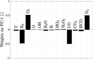
Figure 2: The eigenvector weights $a_{ij}$ associated with the first PC found by PCA on a data set preprocessed with Range scaling.

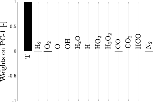
Figure 3: The eigenvector weights $a_{ij}$ associated with the first PC found by PCA on a data set preprocessed with Pareto scaling.

Preprocessing the data set, prior to applying a dimensionality reduction technique, can have a significant impact on the shape of the low-dimensional manifold and on the types of features retrieved from the data set [17], [24]. Figures 2-3 present the weights $a_{ij}$ associated with the first PC resulting from Range and Pareto scaling (see Table 1) of the original data set. Firstly, we observe that the structure of the PC can change significantly with the choice of the scaling technique. If we further consider the mixture fraction variable as defined in eq.(3) as a linear combination of fuel $Y_{F}$ and oxidizer $Y_{O_{2}}$ mass fractions, then it can be observed that the coefficients in front of $Y_{F}$ and $Y_{O_{2}}$ are of opposite signs in that definition. Using Range scaling (Figure 2), the first PC can be attributed to the mixture fraction variable, where the only high weights are for the fuel ($H_{2}$ and $CO$) and oxidizer components ($O_{2}$ and $N_{2}$), and the two have opposite signs. The correlation between the mixture fraction variable and the first PC is $99.96\%$. It is worth noting here, that the mixture fraction was not among the variables in the original data set $\mathbf{X}$ and PCA identifies it in an automatic way. With Pareto scaling (Figure 3), the first PC is almost entirely aligned with the temperature variable and carries almost no information about the mass fractions of the chemical species.

In a previous study [25], the authors have demonstrated that PCA can identify PCs that are independent of the filter width on a fully resolved jet flame. PCA was performed on the state-space variables filtered using a top-hat filter of varying widths. To test the capability of PCA to extract time-invariant features of the data set, we can also use a fixed set of modes to reconstruct new, unseen data, such as data from future time steps of the same temporally evolving system. If the reconstruction process leads to errors that are comparable with the ones obtained for the training data, we can expect that PCA captures the essence of the physical processes underlying the system. We demonstrate this using 2D slices from the DNS data set from four time intervals separated by $\Delta t=5$ms. In Figures 4-5, three future data snapshots (blue triangles) are reconstructed using $q$ first eigenvectors found on the initial snapshot (red circles). Figure 4 shows the coefficients of determination, which can be computed for the $j$th variable $\mathbf{X}_{j}$ in the data set as:

$$R_{j}^{2}=1-\frac{\sum_{i=1}^{N}(x_{ij}-\hat{x}_{ij})^{2}}{\sum_{i=1}^{N}(x_{ij}-\bar{x}_{j})^{2}}$$ (10)

where $x_{ij}$ is the $i$th observation of the $j$th variable, $\hat{x}_{ij}$ is the PCA reconstruction of that observation, and $\bar{x}_{j}$ is the average observation of $\mathbf{X}_{j}$. The coefficient of determination $R^{2}$ measures the goodness of the model fit with respect to fitting the data with the mean value $\bar{x}_{j}$. Values $R^{2}\in(-\infty,1\rangle$, where $R^{2}=1$ means a perfect fit. The smaller the $R^{2}$ value gets, the worse the model fit. Figure 5 shows the normalized root-mean-squared errors (NRMSE) on a logarithmic scale. NRMSE can be computed for the $j$th variable $\mathbf{X}_{j}$ in the data set as:

$$\text{NRMSE}_{j}=\frac{1}{\bar{x}_{j}}\cdot\sqrt{\frac{\sum_{i=1}^{N}(x_{ij}-\hat{x}_{i,j})^{2}}{N}}$$ (11)

In Figures 4-5, the markers represent the mean values of $R^{2}$ or NRMSE averaged over all variables in the data set. The bars range from the minimum and the maximum value achieved for any variable in the data set. It can be observed that for all the reconstructed snapshots, the error metrics show comparable values. This indicates the capability of PCA to capture generalized, time-invariant features of temporally evolving systems. It can also be observed that the mean errors grow for future snapshots, which indicates that there might be a limit on the time separation $\Delta t$ for which we can extend the applicability of the features found.

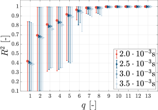
Figure 4: Mean, minimum (worst reconstruction), and maximum (best reconstruction) $R^{2}$ values for reconstructing three snapshots separated by $\Delta t=5$ms (blue triangles) using modes from the snapshot at time $t=2.0\cdot 10^{-3}$s (red circles). Shown for increasing $q$ in the PCA reconstruction.

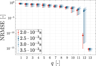
Figure 5: Mean, minimum (best reconstruction), and maximum (worst reconstruction) NRMSE values for reconstructing three snapshots separated by $\Delta t=5$ms (blue triangles) using modes from the snapshot at time $t=2.0\cdot 10^{-3}$s (red circles). Shown for increasing $q$ in the PCA reconstruction.

3.2.2 Local Principal Component Analysis

PCA can also be applied locally (LPCA), on portions of the original data set. In LPCA, the clustering algorithm is first applied to the data set to partition observations into local clusters. Next, PCA is performed separately in each cluster. LPCA can not only allow for further reduction in dimensionality by adjusting to the potential nonlinearities of the data set, but it can also aid in detecting local features of the data. Local PCA can also guide the decision on how to partition the data into clusters, since it grants control of the data reconstruction errors. Figure 6 shows the difference between the global and the local approach on a synthetic data set that is visibly composed of two distinct clusters. In the global case, PCA is performed on the entire data set, ignoring the apparent clusters. When the data set is partitioned and PCA is performed locally in each cluster, a different set of eigenvectors and PCs is tied to each identified cluster of data. Those local PCs can better represent the physics or the underlying features of a particular cluster by capturing the local variance instead of the global one.

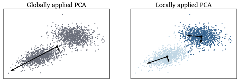
Figure 6: Schematic distinction between global and local PCA on a synthetic 2D data set. The arrows represent the two global/local modes from the matrix $\mathbf{A}$, defining the directions of the largest variance in the global/local data.

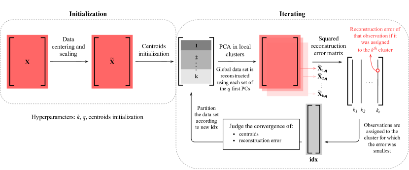
Figure 7: Diagram presenting schematically the VQPCA algorithm.

In LPCA, the $i$th observation $\mathbf{x}_{i}$ is reconstructed from the local, $q$-dimensional manifold in an analogous way to eq.(9):

$$\mathbf{x}_{i}\approx\mathbf{x}_{\mathbf{q},i}=\mathbf{z}_{\mathbf{q},i}(\mathbf{A}_{\mathbf{q}}^{(k)})^{\top}\mathbf{D}+\mathbf{c}^{(k)}$$ (12)

where $k$ is the index of the cluster to which the $i$th observation belongs, $\mathbf{z}_{\mathbf{q},i}$ is the $i$th observation represented in the local, truncated basis $\mathbf{A}_{\mathbf{q}}^{(k)}$ identified on the $k$th cluster. Each cluster is centered separately using the centroid $\mathbf{c}^{(k)}$ of the $k$th cluster and typically the global diagonal matrix of scales $\mathbf{D}$ is applied in each cluster.

Data clustering, prior to applying local PCA, can be performed with any algorithm of choice. One of the techniques discussed in this chapter is the vector quantization PCA (VQPCA) algorithm [26], [27], presented schematically in Figure 7. This is an iterative algorithm in which the observations are assigned to the cluster for which the local PCA reconstruction error of that observation is the smallest. The hyperparameters of the algorithm include: the number of clusters $k$ to partition the data set, the number of PCs $q$ used to approximate the data set at each iteration, and the initial cluster partitioning. The latter is pre-defined by setting the initial cluster centroids. The most straightforward way is to initialize centroids randomly, but another viable option is to use partitioning resulting from a different clustering technique such as K-Means [28]. The algorithm iterates until convergence of the centroids and of the reconstruction error is reached. The reconstruction error is measured between the centered and scaled data set $\widetilde{\mathbf{X}}$ and the approximation $\mathbf{\widetilde{X}}_{\mathbf{i,q}}$ using the $q$ first PCs computed from the eigenvectors found on the $i$th cluster. More details on the VQPCA algorithm can be found in [27] and [7].

Another possible way of clustering the combustion data sets is to use a conditioning variable, such as mixture fraction, and partition the observations based on bins of that variable. If the mixture fraction is used, observations are first split into fuel-lean and fuel-rich parts at the stoichiometric mixture fraction $Z_{st}$. If more than two clusters are requested, lean and rich sides can then be further divided. The approach of performing local PCA on clusters identified through binning the mixture fraction vector is referred to as FPCA.

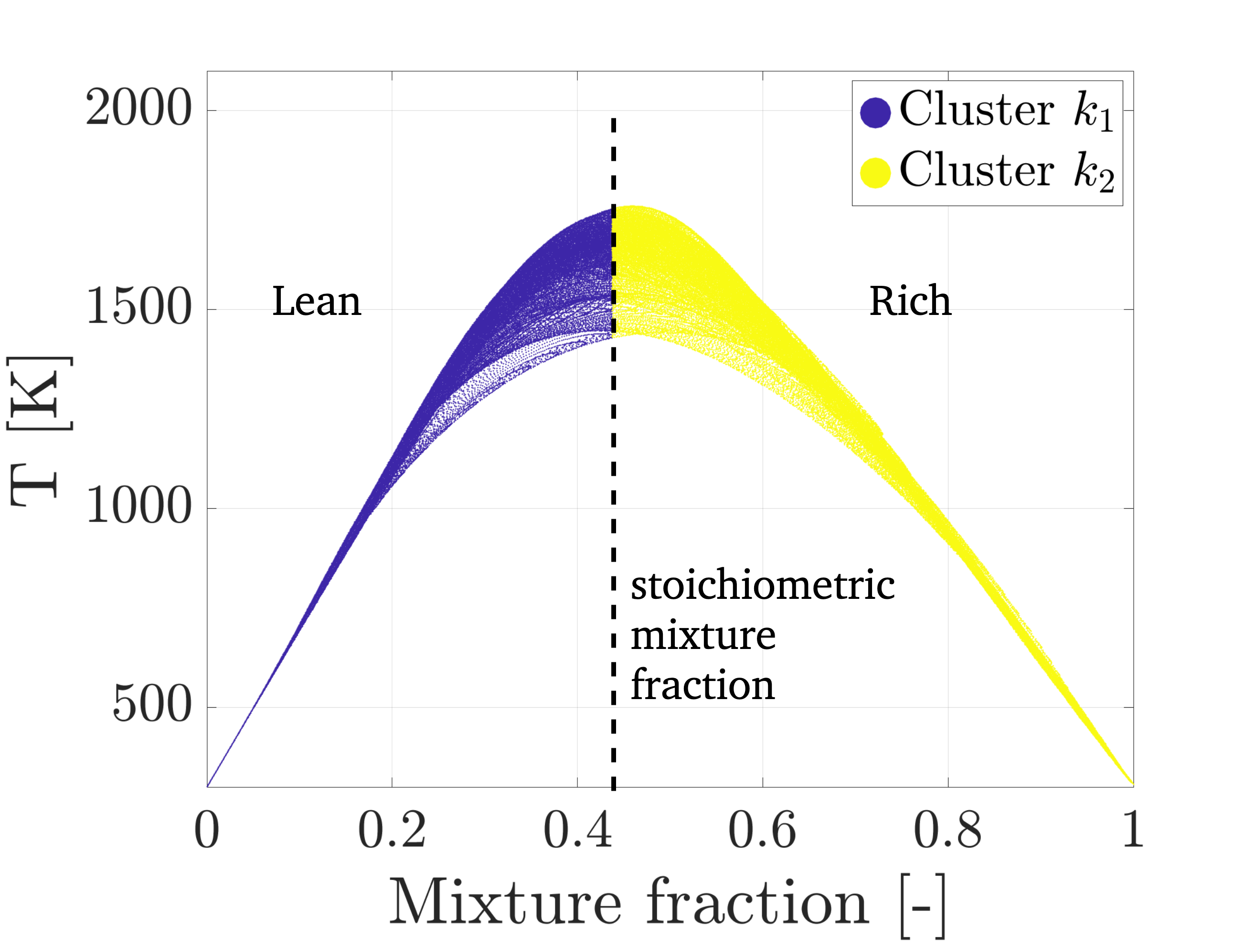
Figure 8: Conditioning variable partitioning into $k=2$ clusters in the mixture fraction-temperature space.

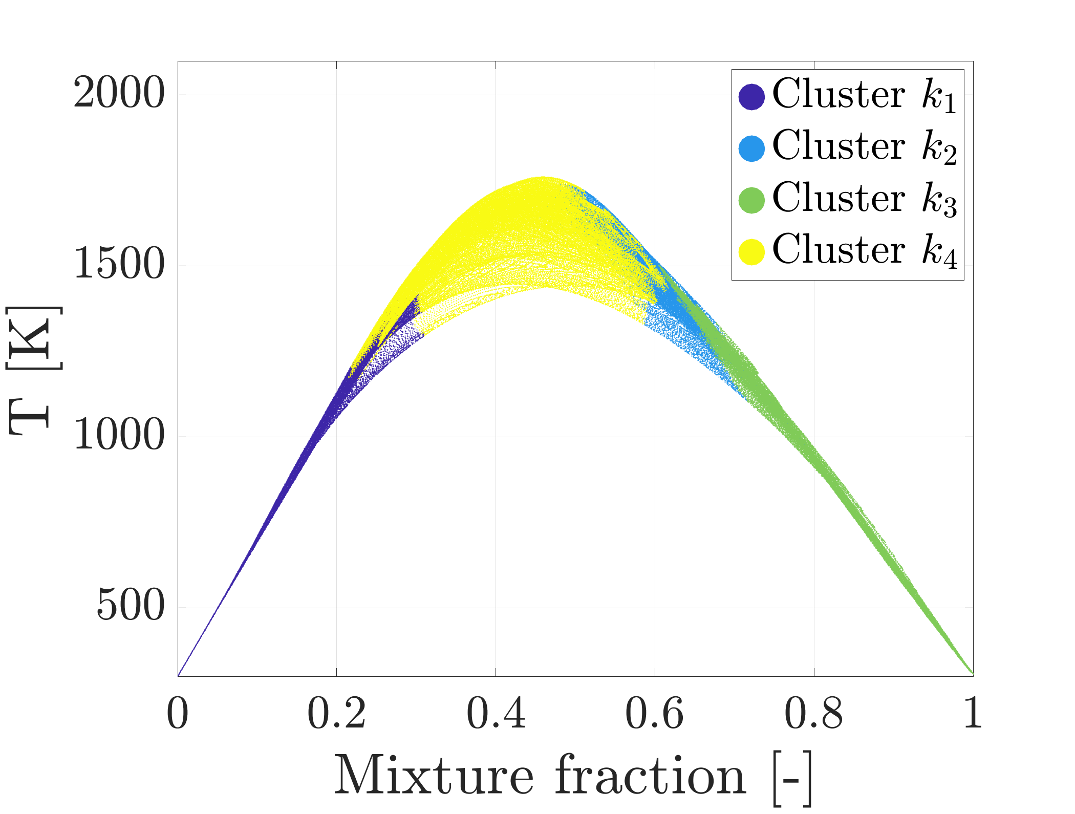
Figure 9: VQPCA partitioning into $k=4$ clusters in the mixture fraction-temperature space.

Local PCA was investigated on the benchmark DNS data set (§3.1) using two clustering algorithms. Figures 8-9 show a comparison between two clustering results in the space of temperature and the mixture fraction variable. Figure 8 presents clustering into $k=2$ clusters using bins of mixture fraction as the conditioning variable. This partitioning can be thought of as hardcoded in a sense that the split into two clusters will always be performed at $Z_{st}$. The features retrieved on local portions of data can thus only be attributed to the lean and rich zones. In contrast, Figure 9 presents clustering into $k=4$ clusters using VQPCA algorithm. The VQPCA method could distinguish between the oxidizer (cluster $k_{1}$), the fuel (cluster $k_{3}$), and the region where the two meet close to stoichiometric conditions (clusters $k_{2}$ and $k_{4}$). This is even more apparent if we plot the result of the VQPCA clustering on a spatial grid in Figure 10. The space is clearly divided into the inner fuel jet ($k_{3}$), the outer oxidizer layer ($k_{1}$), and the two thin reactive layers ($k_{2}$, $k_{4}$) for which the temperature is the highest.

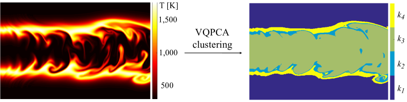
Figure 10: Temperature profile of the DNS data set (left) and the result of partitioning the data set into $k=4$ clusters using the VQPCA algorithm (right).

The success of local PCA in extracting features depends on the clustering technique used. In a previous study [29], VQPCA has been compared to other clustering algorithms, and better results in terms of clustering quality and algorithm speed have been obtained. An unsupervised clustering algorithm based on the VQPCA partitioning has recently been proposed [30] to perform data mining on a high-dimensional DNS data set. If an algorithm such as VQPCA is used, the types of features found depend on data preprocessing and can additionally depend on the hyperparameters. By changing the number of clusters or the number of PCs in the approximation, the user can potentially retrieve different features. This has been also investigated in a previous study [31] for a more complex, high-dimensional DNS data set. This is in contrast with techniques such as binning on the conditioning variable, for which we might have an a priori clarity for what the features will represent.

3.2.3 Non-negative Matrix Factorization

NMF [32] is an algorithm for factorizing data matrices whose elements are non-negative. This technique can thus be applied to the data set as defined in eq.(2) since the thermo-chemical state-space variables are non-negative, provided that at the preprocessing step the data set is scaled but not centered ($\widetilde{\mathbf{X}}=\mathbf{X}\mathbf{D}^{-1}$). That is to ensure that we are not introducing negative elements in the matrix $\widetilde{\mathbf{X}}$ through centering by mean values as is done in eq.(4). Given the non-negative data set $\mathbf{X}\in\mathbb{R}^{N\times Q}$, the scaling matrix $\mathbf{D}$ and the value for $q$, NMF aims to find two non-negative matrices $\mathbf{W}\in\mathbb{R}^{N\times q}$ and $\mathbf{F}\in\mathbb{R}^{q\times Q}$ such that:

$$\mathbf{X}\approx\mathbf{X_{q}}=\mathbf{W}\mathbf{F}\mathbf{D}$$ (13)

The matrix of non-negative factors $\mathbf{F}$ can be regarded as the one containing a basis (analogous to the matrix $\mathbf{A}$ found by PCA). The matrix $\mathbf{W}$ represents the compressed data, namely the NMF scores and is thus analogous to the PCs matrix $\mathbf{Z}$. The factorization to $\mathbf{W}$ and $\mathbf{F}$ is not unique, and various optimization algorithms exist [33], [34]. In this chapter, we use the MATLAB^® routine nnmf, which minimizes the root-mean-squared residual [34]:

$$D=\frac{1}{\sqrt{N\cdot Q}}||\mathbf{X}-\mathbf{W}\mathbf{F}||_{F},$$ (14)

starting with random initial values for $\mathbf{W}$ and $\mathbf{F}$, where the subscript $F$ denotes the Frobenius norm. This optimization might reach local minimum and thus repeating the algorithm can yield different factorizations.

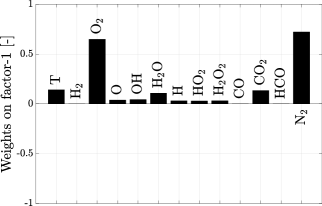
Figure 11: First non-negative factor $\mathbf{f}_{1}$. NMF performed on Range-scaled data with $q=2$.

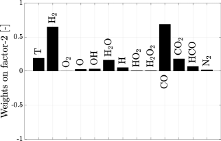
Figure 12: Second non-negative factor $\mathbf{f}_{2}$. NMF performed on Range-scaled data with $q=2$.

Similarly as was done in PCA, we can look at the non-negative factor weights (the elements of $\mathbf{F}$) to assign physical meaning to the factors. With the non-negative constraint on $\mathbf{F}$, only non-negative weights can be found. Figures 11-12 show the first two non-negative factors that together represent the mixture fraction variable (compare with Figure 2). The oxidizer components are included in the first factor and the fuel components in the second. If NMF is compared to PCA, the latter can be thought of as more robust since NMF required two modes to capture the same information (the mixture fraction variable) as was included in a single PCA mode.

3.2.4 Autoencoders

The autoencoder [35], [36] is a type of an unsupervised artificial neural network (ANN) whose aim is to learn the $q$-dimensional representation (embedding) of the $Q$-dimensional data set such that the reconstruction error between the input and the output layer is minimized. The standard form of an autoencoder is the feedforward neural network having an input layer and an output layer with the same number of neurons, and one or more hidden layers. Given one hidden layer, the encoding process takes as an input the preprocessed data matrix $\widetilde{\mathbf{X}}\in\mathbb{R}^{N\times Q}$ and maps it to $\mathbf{H}\in\mathbb{R}^{N\times q}$, with $q<Q$:

$$\mathbf{H}=f(\widetilde{\mathbf{X}}\mathbf{G}+\mathbf{B})$$ (15)

where the columns of $\mathbf{H}$ are referred to as the codes and $f$ is the activation function such as sigmoid, rectified linear unit (ReLU), or squared exponential linear unit (SELU). $\mathbf{G}\in\mathbb{R}^{Q\times q}$ is the matrix of weights and $\mathbf{B}\in\mathbb{R}^{N\times q}$ is the matrix of biases. At the decoding stage, $\mathbf{H}$ is mapped to the reconstruction $\widetilde{\mathbf{X}}_{\mathbf{q}}$:

$$\widetilde{\mathbf{X}}\approx\widetilde{\mathbf{X}}_{\mathbf{q}}=f^{\prime}(\mathbf{H}\mathbf{G^{\prime}}+\mathbf{B^{\prime}})$$ (16)

where $f^{\prime}$, $\mathbf{G^{\prime}}$, and $\mathbf{B^{\prime}}$ may be unrelated to $f$, $\mathbf{G}$, and $\mathbf{B}$. The encoding/decoding process can thus be summarized as:

$$\widetilde{\mathbf{X}}\in\mathbb{R}^{N\times Q}\xrightarrow{\text{encoding}}\mathbf{H}\in\mathbb{R}^{N\times q}\xrightarrow{\text{decoding}}\widetilde{\mathbf{X}}_{\mathbf{q}}\in\mathbb{R}^{N\times Q}$$ (17)

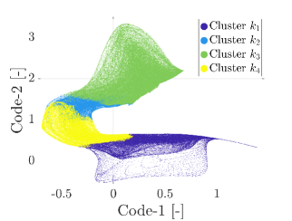
Figure 13: 2D manifold obtained using an Autoencoder with five hidden layers and SELU activation function. Colored by the result of VQPCA partitioning into $k=4$ clusters.

In this section, we use an autoencoder with five hidden layers and SELU activation function and generate a 2D embedding ($q=2$) of the original data set. Figure 13 shows the 2D manifold obtained after the autoencoder compression (represented by the matrix $\mathbf{H}$). The manifold is colored by the previously obtained result of partitioning via the VQPCA algorithm. From Figure 13, it can be observed that the result of VQPCA partitioning still uniformly divides the autoencoder manifold. Clusters $k_{1}$ and $k_{3}$, representing the oxidizer and fuel respectively, are located at the opposing ends of the manifold. Thus, it is possible to think of that manifold as describing the progress of the combustion process, with the fuel and oxidizer meeting in the center ($k_{2}$ and $k_{3}$) where they finally react.

3.2.5 Linear Operations That Aid in Feature Interpretation

Several linear operations can aid in the interpretation of PCs or low-dimensional manifolds. One of such techniques is the rotation of modes/factors [37], [23] with the varimax orthogonal rotation [38] used most commonly. In the varimax rotation, we first select which $n$ factors should be rotated together. It then maximizes the sum of variances of the squared weights within each of the $n$ rotated factors:

$$\mathcal{V}=\sum(w_{ij}^{2}-\bar{w}_{ij}^{2})^{2}$$ (18)

where $w_{ij}$ is the $i$th weight on the $j$th factor and $\bar{w}_{ij}^{2}$ is the mean of the squared weights [37]. After rotation, those $n$ factors explain the same total amount of variance as they did together before the rotation, but variance is now redistributed differently among the selected factors. Varimax-rotated factors typically have high weights on fewer variables than the original factors, and that can aid in their physical interpretation. The rotated factors can then be used as the new basis to represent the original data set. Varimax and several other rotation methods are available within the MATLAB^® routine rotatefactors.

Another interesting technique is the Procrustes analysis [39], which is a series of linear operations that allow translation, rotation, or scaling of the low-dimensional manifold. This can be particularly useful when manifolds obtained from two dimensionality reduction techniques should be compared. Figures 14-15 present the Procrustes transformation (using the MATLAB^® routine procrustes) of the LPCA manifold onto an autoencoder manifold. With the series of linear transformations the manifolds overlay each other, and the match between them becomes closer to exact as the number of clusters with which VQPCA was performed is increased. This suggests that the data reconstruction error for the 2D approximation from LPCA will approach the one from autoencoder decoding when the number of clusters is high enough.

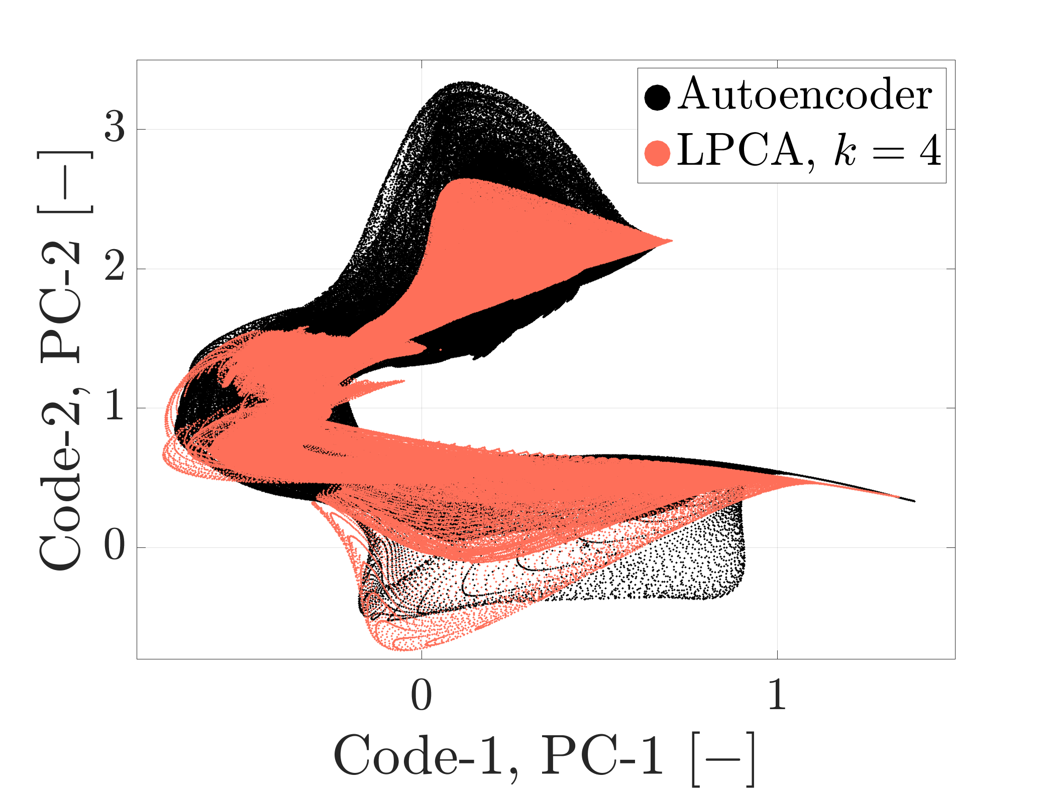
Figure 14: The 2D manifold obtained from local PCA using VQPCA clustering algorithm and increasing the number of clusters, overlayed with the autoencoder manifold using the Procrustes analysis. VQPCA performed with $k=4$ clusters.

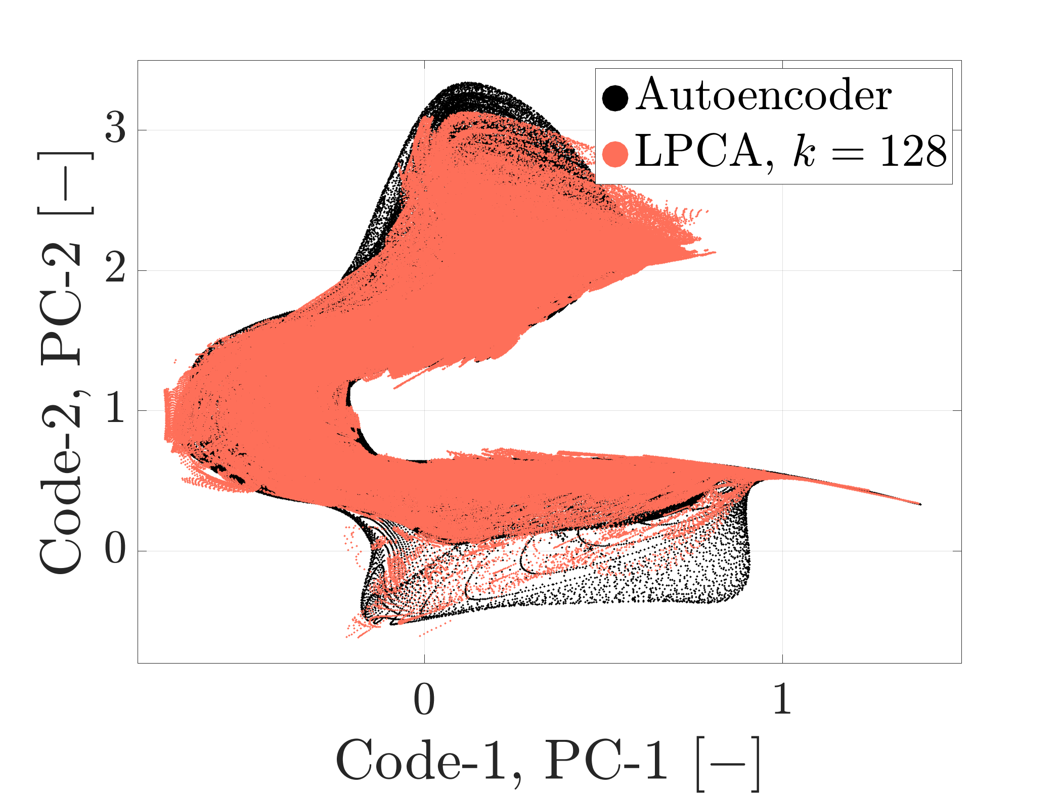
Figure 15: The 2D manifold obtained from local PCA using VQPCA clustering algorithm and increasing the number of clusters, overlayed with the autoencoder manifold using the Procrustes analysis. VQPCA performed with $k=128$ clusters.

4 Transport of Principal Components

In §2, we have seen that the number of thermo-chemical state-space variables $Q$ determines the original dimensionality of the data set. This number also reflects how many transport equations for the state-space variables should be solved in a numerical simulation. The general transport equation for the set $\mathbf{\Phi}=\mathbf{X}^{\top}=[T,p,Y_{1},Y_{2},\dots,Y_{N_{s}-1}]^{\top}$ of state-space variables is:

$$\rho\frac{D\mathbf{\Phi}}{Dt}=-\nabla\cdot(\mathbf{j_{\Phi}})+\mathbf{S_{\Phi}}$$ (19)

where $\mathbf{j_{\Phi}}$ is the mass-diffusive flux of $\mathbf{\Phi}$ relative to the mass-averaged velocity, and $\mathbf{S_{\Phi}}$ is the volumetric rate of production of $\mathbf{\Phi}$ (also referred to as the source of $\mathbf{\Phi}$). Performing detailed simulations with large chemical mechanisms with significant number of chemical species is still computationally prohibitive. In [40], the authors proposed to use PCA to reduce the number of transport equations that solve a combustion process. Instead of solving the original set of $Q$ transport equations, the original variables are first transformed to the new basis identified by PCA on the training data set $\mathbf{X}$. Next, the truncation from $Q$ to $q$ first PCs is performed. Transport equations for the $q$ first PCs can be formulated from eq.(19) using the truncated basis matrix $\mathbf{A_{q}}$:

$$\rho\frac{D\mathbf{z}}{Dt}=-\nabla\cdot(\mathbf{j_{z}})+\mathbf{S_{z}}$$ (20)

where $\mathbf{z}=\mathbf{Z_{q}}^{\top}$ (with $\mathbf{Z_{q}}=(\mathbf{X}-\mathbf{\bar{X}})\mathbf{D}^{-1}\mathbf{A_{q}}$), $\mathbf{j_{z}}=\mathbf{A_{q}}\mathbf{j_{\Phi}}$, and $\mathbf{S_{z}}=\mathbf{A_{q}}\mathbf{S_{\Phi}}\mathbf{D}^{-1}$ (also referred to as the PC-sources). This is the discrete analog of the Galerkin projection methods described in Chapters 6 and 14. Note that the source terms of the PCs, $\mathbf{S_{z}}$, are scaled (but not centered) using the same scaling matrix $\mathbf{D}$ as applied on the data set $\mathbf{X}$.

The challenge associated with the resolution of the PC-transport equation is related to the PC-source terms. The latter are highly nonlinear functions (based on Arrhenius expressions) of the state space variables. The nonlinearity of the chemical source terms strongly impacts the degree of reduction attainable using the projection of the species transport equations onto the PCA basis [41], [42]. A solution to this problem is to use PCA to identify the most appropriate basis to parameterize the ELDM and then, both the thermo-chemical state-space variables and the PC-source terms can be nonlinearly regressed onto the new basis. This allows to overcome the shortcomings associated with the multi-linear nature of PCA and to reduce the number of components required for an accurate description of the state-space.

The construction of an appropriate low-dimensional manifold requires training data. This might be seen as a limitation of the approach since all system states are required before applying model reduction. Although initial studies on PCA models involved DNS data of turbulent combustion [40], [1], recent studies have demonstrated [43], [44], [45], [46], [47] that PCA-based models can be trained on simple and inexpensive systems, such as zero-dimensional reactors and one-dimensional flames (see §2), and then applied to model complex systems, such as the flame-vortex interaction [48], the flame-turbulence interaction [42] as well as the turbulent premixed [45] and non-premixed flames [49]. Up-to-date, the PC-transport approach has been demonstrated for a wide range of problems involving ideal reactors, including batch and PSR reactors.

4.1 Non-linear Regression Models

The thermo-chemical state-space variables $\mathbf{\Phi}$ and the PC-source terms $\mathbf{S_{Z_{q}}}$ can be mapped to the $q$-dimensional PC space using a nonlinear regression function $\mathscr{F}$, such that:

$$\phi\approx\mathscr{F}(\mathbf{Z_{q}})$$

where $\phi$ represents any of the dependent variables ($T,p,Y_{1},Y_{2},\dots,Y_{N_{s}-1}$, or $\mathbf{S_{Z_{q}}}$). The models used in the literature to generate the function $\mathscr{F}$ include, but are not limited to:

• multivariate adaptive regression splines (MARS) [50],

• artificial neural networks (ANN) [51],

• Gaussian process regression (GPR) [52].

In a previous study [42], the authors compared different regression models in their ability to accurately map highly nonlinear functions (such as the chemical source terms) to the PCA manifold. In this section, we will focus on the use of GPR for state-space and source term parameterization. The choice of GPR is due to its semi-parametric nature that increases the generality of the approach. GPR employs Gaussian mixtures to capture information about the relation between data and input parameters, making predictions of non-observed system states more reliable than in fully parametric approaches.

4.2 Validation of the PC-Transport Approach in LES Simulations

To demonstrate the application of the PC-transport approach, we show the results of the LES of a multi-dimensional flame [49]. A piloted methane-air diffusion flame (referred to as Flame D) [53] for which high-fidelity experimental data is available is selected. Flame D is fueled by a mixture of $CH_{4}$ and air ($25\%\ /\ 75\%$ by volume), at $Re=22,400$ and 294K, respectively. The fuel jet is surrounded by pilot flames that stabilize the flame. Finally, an air co-flow surrounds the flame.

The development of a reduced-order model for subsequent application in LES requires the availability of training data. The most critical aspect when generating a training data set is to make sure that the generated state-space includes all the possible states accessed during the actual simulation. At the same time, that data cannot come from expensive simulations. Parametric calculations on inexpensive canonical configurations can provide an effective solution in this context, although the nature of the flame archetype chosen is an open subject of discussion. Considering the non-premixed nature of Flame D, it was decided to rely on unsteady one-dimensional laminar counter diffusion flames. The use of unsteady inlet velocity profiles allows to explore transient flame behavior, including extension and re-ignition phenomena. The calculations were performed using the OpenSMOKE++ suite developed in Politecnico di Milano [54]. The GRI 3.0 [55] mechanism, involving 35 species and 253 reactions (excluding $NO_{x}$), was used. The inlet conditions were set equal to the experimental ones [53]. Multiple simulations were carried out by varying the strain rate, from equilibrium to complete extinction. The unsteady solutions were saved on a uniform grid of 400 points over a $0.15$ m domain. All of the unsteady data from the various simulations was used collectively for the PCA analysis. The final data set consisted of $\sim 80,000$ observations for each of the state-space variables.

Table 2: The elements $a_{ij}$ of the basis matrix $\mathbf{A}$ identified by PCA when the data set was composed of five major chemical species only.

Species	$\mathbf{A}_{1}$	$\mathbf{A}_{2}$	$\mathbf{A}_{3}$	$\mathbf{A}_{4}$	$\mathbf{A}_{5}$
$H_{2}O$	-0.02	0.51	0.45	-0.73	0.02
$O_{2}$	-0.18	-0.67	-0.22	-0.60	0.30
$N_{2}$	-0.64	-0.01	-0.15	-0.09	-0.74
$CH_{4}$	0.73	-0.14	-0.20	-0.27	-0.56
$CO_{2}$	-0.02	0.50	-0.82	-0.14	0.21

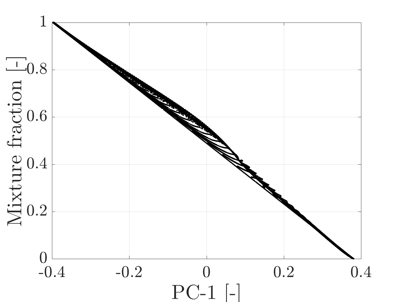
Figure 16: Scatter plot of the first PC (PC-1) versus the mixture fraction variable. Reprinted from [49] with permission from Elsevier.

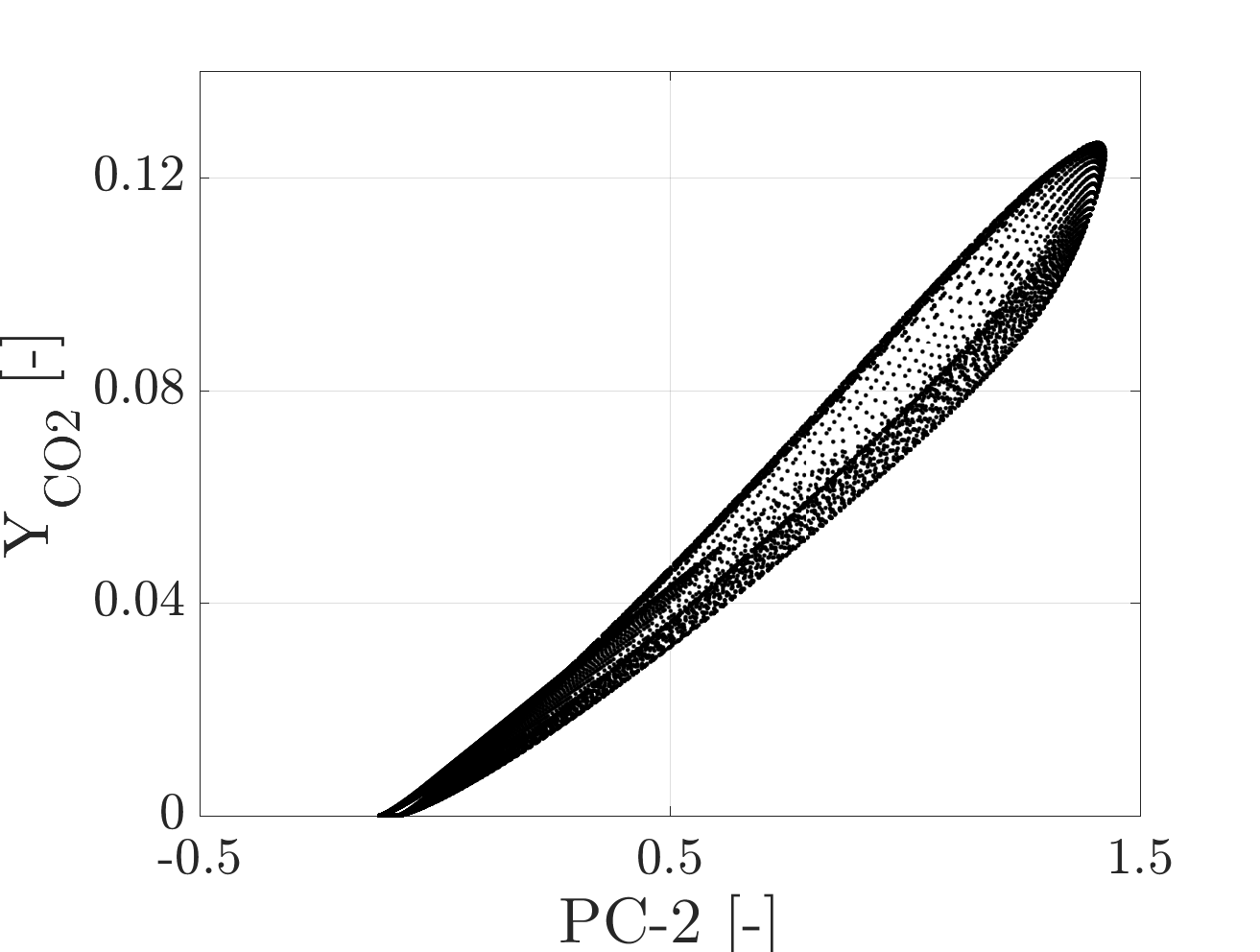
Figure 17: Scatter plot of the second PC (PC-2) versus the mass fraction of $CO_{2}$ species, $Y_{CO_{2}}$. Reprinted from [49] with permission from Elsevier.

Table 2 shows the basis matrix weights obtained from the PCA analysis on the five major chemical species only. It can be seen that $\mathbf{Z}_{1}$ has a large positive weight for $CH_{4}$ and a large negative value for the oxidizer ($O_{2}$ and $\mathrm{N_{2}}$). This can be linked to the definition of mixture fraction from eq.(3). Figure 16 shows a plot of the first PC highly correlated with the mixture fraction (correlation factor exceeding 99%). Therefore, in the numerical simulation, the first PC is directly replaced by the mixture fraction, to avoid transporting a reactive scalar. The weights for $\mathbf{Z}_{2}$ also show an interesting pattern: a positive correlation for $H_{2}O$ and $CO_{2}$, and a negative correlation for $CH_{4}$, $O_{2}$, and $N_{2}$. This can be linked to a progress variable, where products have positive stoichiometric coefficients and reactants negative ones. Figure 17 shows a plot of the second PC highly correlated with the mass fraction of $CO_{2}$, a variable that can be attributed to the progress of reaction. It is worth pointing out that PCA identifies these patterns without any prior assumptions or knowledge of the system of interest.

LES simulations were then performed in OpenFOAM using the PC-transport approach. The independent variables (PCs) are transported, and the state-space is recovered from the nonlinear regression using GPR. The low-Mach Navier-Stokes equations are solved on an unstructured grid, together with the PC-transport equations from eq.(20). Since the state-space was accurately regressed using $q=2$ PCs, the simulation was carried out using only $\mathbf{Z}_{1}$ and $\mathbf{Z}_{2}$ as transported PCs. More details about the numerical setting are reported in [49]. As part of the validation of the method, we look at the temperature profiles conditioned on mixture fraction at axial location $x/D=60$ ($x=432$mm), shown in Figure 18. It can be observed that the predicted temperature lies well inside the single shot experimental data points.

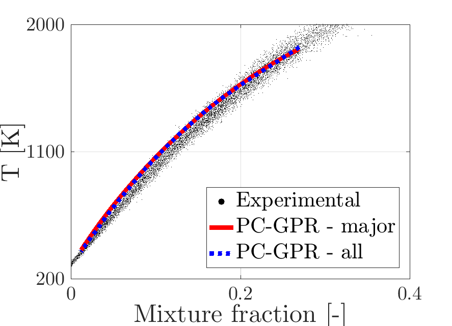
Figure 18: Conditional average of the temperature at $x/D=60$. Reprinted from [49] with permission from Elsevier.

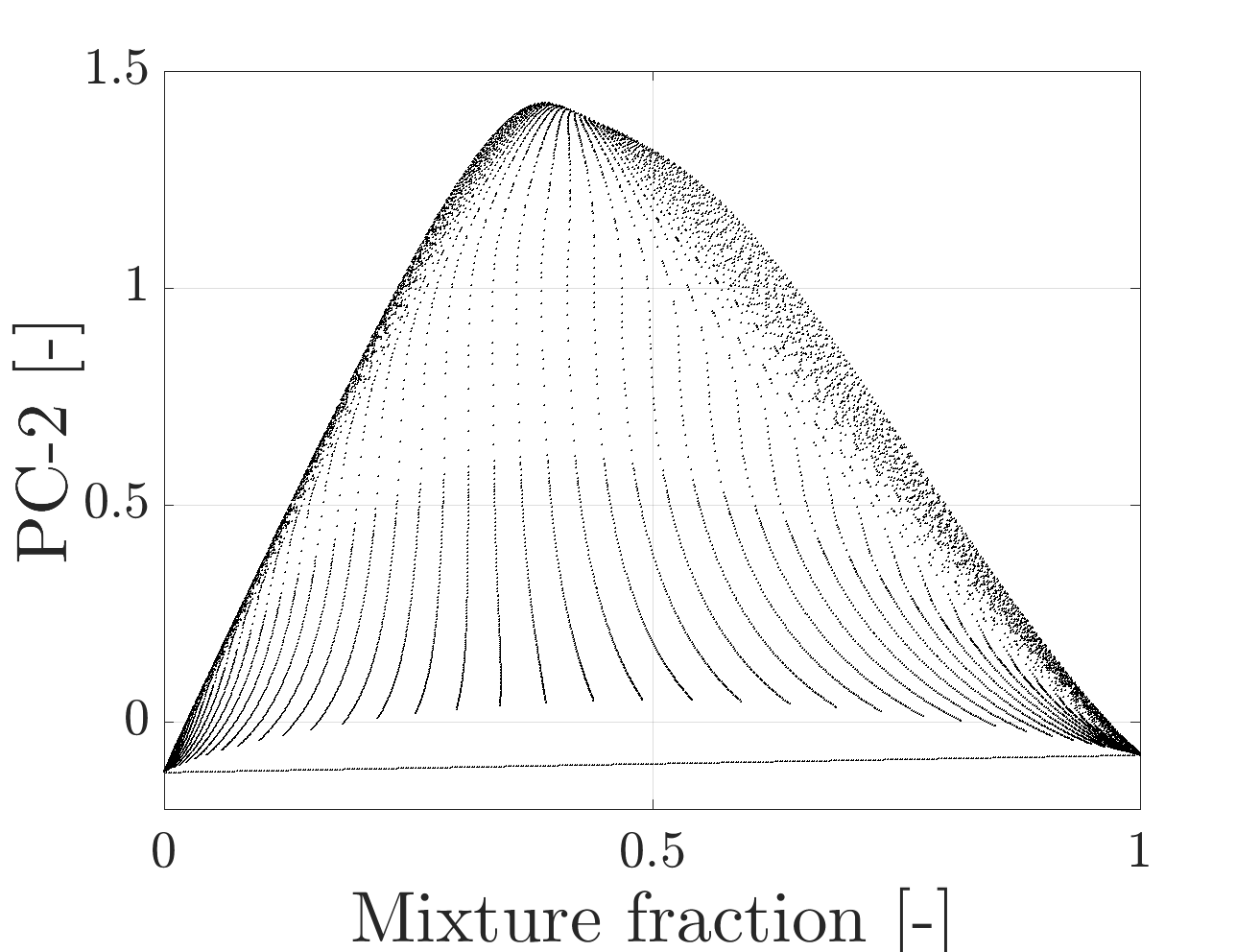
Figure 19: Scatter plot of the low-dimensional combustion manifold in the space of the second PC (PC-2), and the mixture fraction variable. Manifold obtained from the training data set. Reprinted from [49] with permission from Elsevier.

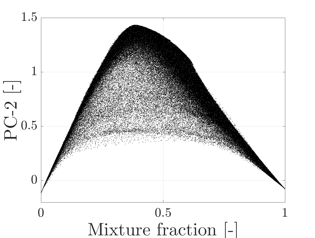
Figure 20: Scatter plot of the low-dimensional combustion manifold in the space of the second PC (PC-2), and the mixture fraction variable. Manifold accessed during the simulation. Reprinted from [49] with permission from Elsevier.

Figure 19 shows the original manifold obtained from the training data set, while Fig. 20 shows the manifold accessed during the simulation with major species at $t=1s$. It can be observed that the simulation does not leave the training manifold, all the points accessed are bounded inside the original training manifold. It is also apparent that most of the solution data is clustered toward the equilibrium solution, showing that the Flame D does not experience significant extinction and re-ignition.

The PC-GPR model can accurately simulate a complex multi-dimensional flame, using only 2 PCs instead of the 35 chemical species. The model can be built using inexpensive one-dimensional simulations, as long as the training data covers the potential state-space accessed during the actual simulation. The PCs stay bounded to the training manifold during the simulation, indicating that the choice of an unsteady canonical reactor ensures to span all the potential chemical states accessed during the simulation. The strength of the method resides in the fact that it does not require any prior selection of variables. Instead, it automatically extracts the most relevant variables to describe the system. From this perspective, the PC-GPR method can be regarded as a generalization of tabulated chemistry approaches [1], particularly for complex systems requiring the definition of a larger number of progress variables.

5 Chemistry Acceleration via Adaptive-Chemistry

In §4, PCA was used to derive the reduced number of transport equations for the new set of variables, PCs. Regression was introduced to handle the nonlinearity of chemical source terms. In this section, we investigate the potential of local PCA (§3.2.2) to classify the thermo-chemical state-space into locally homogeneous regions and apply chemical mechanism reduction locally.

5.1 Description of the Approach

In [56], the authors proposed the operator-splitting strategy for application in numerical algorithms used to solve the multi-component reactive flows. With this approach, chemistry acceleration techniques can be implemented to reduce the computational cost related to the inclusion of detailed kinetic mechanisms. If we consider $\mathbf{\Psi}$ as a vector representing the temperature and mass fractions of chemical species, the transport equation for $\mathbf{\Psi}$ can be written as:

$$\frac{d\mathbf{\Psi}}{dt}=\mathbf{C}(\mathbf{\Psi},t)+\mathbf{D}(\mathbf{\Psi},t)+\mathbf{S}(\mathbf{\Psi})$$ (21)

where $\mathbf{C}(\mathbf{\Psi},t)$ and $\mathbf{D}(\mathbf{\Psi},t)$ are the convective and diffusive transport terms, respectively, and $\mathbf{S}(\mathbf{\Psi})$ is the source term vector (representing the rates of change of $\mathbf{\Psi}$ due to chemical reactions) [57]. For $N$ grid points in the simulation, we obtain a system of $N$ ordinary differential equations (ODEs). According to the Strang splitting scheme [58], eq.(21) can be solved by grouping the contributions of convection and diffusion and integrating them separately from the chemical source term:

$$\begin{cases}\frac{d\mathbf{\Psi}^{a}}{dt}=\mathbf{S}(\mathbf{\Psi}^{a})\\ \frac{d\mathbf{\Psi}^{b}}{dt}=\mathbf{C}(\mathbf{\Psi}^{b}{,t})+\mathbf{D}(\mathbf{\Psi}^{b}{,t})\end{cases}$$ (22)

where the indices $a$ and $b$ denote the separate contributions to $\mathbf{\Psi}$. In particular, three sub-steps are adopted for the numerical integration:

1. Reaction step: The ODE system corresponding to the source term $\mathbf{S}(\mathbf{\Psi}^{a})$ is integrated over $\frac{\Delta t}{2}$.

2. Transport step: The ODE system accounting for the convection and diffusion terms $\mathbf{C}(\mathbf{\Psi}^{b},t)$ and $\mathbf{D}(\mathbf{\Psi}^{b},t)$ is integrated over $\Delta$t.

3. Reaction step: The source term $\mathbf{S}(\mathbf{\Psi}^{a})$ is again integrated over $\frac{\Delta t}{2}$.

Unlike the transport step, the two reaction steps do not require any boundary conditions and they do not have any spatial dependence. The system of $N$ ODEs from steps 1 and 3 can be solved independently from the system of $N$ ODEs from step 2. This makes the adaptive-chemistry techniques very effective and easy to implement. The idea behind the adaptive-chemistry approach is that it is possible to locally consider only a subset of the chemical species implemented in the detailed mechanism, while the remaining subset consists of the species that locally have zero concentration, or result to be not chemically active. It is thus possible to build a library of reduced mechanisms in the preprocessing step, covering the composition space, which is expected to be visited during simulation of the flame of interest [59], [60]. To build the library of reduced mechanisms, the state-space must be first partitioned into a prescribed number of clusters, and a reduced kinetic mechanism is then created separately in each cluster. The high-dimensional space can be partitioned via the VQPCA algorithm (§3.2.2), and for each cluster a reduced kinetic mechanism is generated via directed relation graph with error propagation (DRGEP) [61]. At each time-step of the CFD simulation, the whole set of species in the detailed mechanism is transported. Before the chemical step, the grid points are classified on-the-fly using the local PCA reconstruction error metrics [26], and for each of them the appropriate reduced mechanism is selected from the library. Although a direct relation between the CPU time and the number of species implemented in the mechanism is found for both the transport and the reaction sub-steps described in the eq.(22), alleviating the costs related to the reaction step appears to be more important. The reaction step, in fact, results to be the most consuming part of the computation requiring up to 80 - 85% of the CPU time [57]. The full details of the overall procedure, called SPARC, as well as its validation for steady and unsteady laminar flames, can be found in [62].

5.2 Application of the Approach

Figure 21: Temperature, $O_{2}$, $OH$ and $CO$ profiles obtained from the detailed and the adaptive-chemistry simulation of an axisymmetric, non-premixed laminar nitrogen-diluted methane coflow flame.

The application of the adaptive-chemistry approach is briefly presented here for the simulation of an axisymmetric, non-premixed laminar nitrogen-diluted methane co-flow flame [63]. The detailed simulation was first carried out using the POLIMI_C1C3_HT_1412 kinetic mechanism (84 species and 1698 reactions) [64], and the adaptive simulations were then performed using four degrees of chemical reduction, ranging from $\epsilon_{DRGEP}=0.03$ to $\epsilon_{DRGEP}=0.005$. The average and the maximum number of species included in the reduced mechanisms depending on the reduction tolerance $\epsilon_{DRGEP}$ are reported in Table 3. An excellent agreement was observed for all the cases, although for $\epsilon_{DRGEP}=0.03$ and 0.02 a negligible discrepancy was observed for the lift-off height. The inverse proportionality between the simulation accuracy and the degree of reduction, i.e., the tolerance used for DRGEP, is due to a different number of species included in the reduced mechanisms. Figure 21 shows a comparison between the temperature and species profiles obtained from the detailed and the adaptive simulation carried out with $\epsilon_{DRGEP}=0.005$.

Table 3: The mean and maximum number of chemical species versus the uniformity coefficients for prescribed tolerances $\epsilon$ in DRGEP. The composition space was partitioned via the VQPCA algorithm.

$\epsilon_{DRGEP}$	$n_{sp}^{mean}$	$n_{sp}^{max}$
0.03	31	38
0.02	34	42
0.01	39	44
0.005	43	50

The inclusion of a higher number of chemical species in the reduced mechanisms obviously entails an increase of the mean CPU-time required to carry out the chemical step ($\bar{\tau}_{chem}$). Nevertheless, the adaptive simulation speed-up with respect to the detailed simulation ($S_{chem}$) is large ($S_{chem}\sim 4$) even when the lowest degree of chemical reduction is adopted, as reported in Table 4.

Table 4: Performances of adaptive-chemistry algorithm: average CPU-time per cell (in $ms$) for chemical step integration ($\bar{\tau}_{chem}$) and relative mean speed-up factor ($S_{chem}$) for the steady-state laminar methane flame with respect to the degree of chemistry reduction ($\epsilon_{DRGEP}$).

$\epsilon_{DRGEP}$	$\bar{\tau}_{chem}$	$S_{chem}$
0.03	2.78	5.39
0.02	3.03	4.94
0.01	3.25	4.61
0.005	3.78	3.97
detailed	15.02	-

If multi-dimensional simulations of the same system are not available, the SPARC model can be trained using lower-dimensional (0D or 1D) detailed simulations of the same chemical system. Reduced mechanisms can then be generated based on such training data sets and applied in the multi-dimensional (2D or 3D) adaptive simulations. In [62], a data set consisting of observations generated through steady-state CFDF simulations (see §2), evaluated at different strain rates from $10s^{-1}$ to $330s^{-1}$ (the latter corresponding to extinction conditions) was also considered. This new data set consisted of $\sim 11,000$ points, corresponding to $30$ different strain rates randomly chosen in the considered interval. Also in this case, the accuracy using mechanisms obtained from a lower dimensional training data set was high, with the speed-up with respect to the detailed simulation between 4.5 and 6. More details can be found in [62].

6 Available Software

Apart from the many available MATLAB^® routines, some of which were mentioned in this chapter, two recently developed Python libraries can be used to perform data-driven ROM:

• OpenMORe [65] is a collection of Python modules for reduced-order modeling (ROM), clustering, and classification. It incorporates many ROM techniques such as: PCA, local PCA, kernel PCA and NMF along with the varimax rotation for factor analysis. It can also be used for data clustering with VQPCA or FPCA algorithms, and it introduces utilities for evaluating the clustering solutions. The software, along with a detailed documentation and several examples, is available at https://github.com/burn-research/OpenMORe.

• PCAfold [66] is a Python library that can be used to generate, improve and analyze low-dimensional manifolds obtained via PCA. Several novel functionalities to perform PCA on sampled data sets and analyzing the improved representation of the thermo-chemical state-space variables [67] were introduced. The effect of the training data preprocessing on the topology of the low-dimensional manifolds can be investigated with the novel approaches and metrics to assess the quality of manifolds [68], [69], [70]. PCAfold also accommodates for treatment of the thermo-chemical source terms for use in PC-transport approaches (§4). The user can find numerous illustrative examples and the associated Jupyter notebooks in the software documentation (available at https://pcafold.readthedocs.io/) under Tutorials & Demos. The software is available at https://gitlab.multiscale.utah.edu/common/PCAfold.

7 Summary

In this chapter, several examples of the application of data-driven techniques to multi-component reactive flow systems have been shown. Data reduction techniques, such as PCA, NMF or autoencoders also offer a way to explore hidden features of data sets (§3). These methods are capable of detecting information in an unsupervised way and can thus aid in the process of selecting the best set of variables to effectively parameterize complex systems using fewer dimensions. Moreover, it has been shown how the aforementioned algorithms can be effectively coupled with algorithms that are widely used in the combustion community, such as DRGEP, to obtain physics-informed reduced-order models. Two applications of reduced-order modeling were presented in this chapter: reduction of the number of transport equations (§4) and reduction of large chemical mechanisms (§5). The main power of data-driven techniques is that the modeling can be informed by applying the technique on simple systems that are computationally cheap to obtain. Further improvement can be achieved based on the feedback coming from the validation experiments.

References

- [1] Stephen B. Pope. Small scales, many species and the manifold challenges of turbulent combustion. Proceedings of the Combustion Institute, 34(1):1–31, 2013.
- [2] A. Frassoldati, T. Faravelli, and E. Ranzi. Kinetic modeling of the interactions between NO and hydrocarbons at high temperature. Combustion and Flame, 135:97–112, 2003.
- [3] K.K. Kuo and R. Acharya. Fundamentals of Turbulent and Multi-Phase Combustion. Wiley, 2012.
- [4] B. F. Magnussen. On the structure of turbulence and a generalized eddy dissipation concept for chemical reaction in turbulent flow. 19th AIAA Aerospace Science Meeting, 1981.
- [5] A. Cavaliere and M. de Joannon. Mild combustion. Progress in Energy and Combustion Science, 30:329–366, 2004.
- [6] J.Wünning and J.Wünning. Flameless oxidation to reduce thermal NO-formation. Progress in Energy and Combustion Science, 23:81–94, 1997.
- [7] A. Parente, J.C. Sutherland, B.B. Dally, L. Tognotti, and P.J. Smith. Investigation of the MILD combustion regime via Principal Component Analysis. Proceedings of the Combustion Institute, 33(2):3333–3341, 2011.
- [8] Tianfeng Lu and Chung K Law. Toward accommodating realistic fuel chemistry in large-scale computations. Progress in Energy and Combustion Science, 35(2):192–215, 2009.
- [9] R.W. Bilger, S.H. Starner, and R.J. Kee. On reduced mechanisms for methane-air combustion in nonpremixed flames. Combustion and Flame, 80:135–149, 1990.
- [10] Norbert Peters. Laminar diffusion flamelet models in non-premixed turbulent combustion. Progress in Energy and Combustion Science, 10(3):319–339, 1984.
- [11] Chung K Law. Combustion physics. Cambridge University Press, 2010.
- [12] Alan R Kerstein. One-dimensional turbulence: model formulation and application to homogeneous turbulence, shear flows, and buoyant stratified flows. Journal of Fluid Mechanics, 392:277–334, 1999.
- [13] Tarek Echekki, Alan R Kerstein, and James C Sutherland. The one-dimensional-turbulence model. In Turbulent Combustion Modeling, pages 249–276. Springer, 2011.
- [14] Joel H Ferziger, Milovan Perić, and Robert L Street. Computational methods for fluid dynamics, volume 3. Springer, 2002.
- [15] Robert J Kee, Michael E Coltrin, and Peter Glarborg. Chemically reacting flow: theory and practice. John Wiley & Sons, 2005.
- [16] Stephen R Turns et al. Introduction to combustion, volume 287. McGraw-Hill Companies, 1996.
- [17] Alessandro Parente and James C. Sutherland. Principal component analysis of turbulent combustion data: Data pre-processing and manifold sensitivity. Combustion and Flame, 160(2):340–350, 2013.
- [18] Yue Yang, Stephen B. Pope, and Jacqueline H. Chen. Empirical low-dimensional manifolds in composition space. Combustion and Flame, 160(10):1967–1980, 2013.
- [19] James C. Sutherland, Philip J. Smith, and Jacqueline H. Chen. A quantitative method for a priori evaluation of combustion reaction models. Combustion Theory and Modelling, 11(2):287–303, 2007.
- [20] Richard A Yetter, FL Dryer, and H Rabitz. A comprehensive reaction mechanism for carbon monoxide/hydrogen/oxygen kinetics. Combustion Science and Technology, 79(1-3):97–128, 1991.
- [21] I.T. Jolliffe. Principal Component Analysis. Springer-Verlag New York, 2002.
- [22] Carl Eckart and Gale Young. The approximation of one matrix by another of lower rank. Psychometrika, 1(3):211–218, 1936.
- [23] Aurélie Bellemans, Gianmarco Aversano, Axel Coussement, and Alessandro Parente. Feature extraction and reduced-order modelling of nitrogen plasma models using principal component analysis. Computers & Chemical Engineering, 115:504–514, 2018.
- [24] Kim Peerenboom, Alessandro Parente, Tomáš Kozák, Annemie Bogaerts, and Gérard Degrez. Dimension reduction of non-equilibrium plasma kinetic models using principal component analysis. Plasma Sources Science and Technology, 24(2):025004, 2015.
- [25] Amir Biglari and James C. Sutherland. A filter-independent model identification technique for turbulent combustion modeling. Combustion and Flame, 159(5):1960–1970, 2012.
- [26] Nandakishore Kambhatla and Todd K Leen. Dimension reduction by local principal component analysis. Neural Computation, 9(7):1493–1516, 1997.
- [27] A. Parente, J.C. Sutherland, L. Tognotti, and P.J. Smith. Identification of low-dimensional manifolds in turbulent flames. Proceedings of the Combustion Institute, 32(1):1579–1586, 2009.
- [28] James MacQueen et al. Some methods for classification and analysis of multivariate observations. In Proceedings of the fifth Berkeley symposium on mathematical statistics and probability, volume 1, pages 281–297. Oakland, CA, USA, 1967.
- [29] Giuseppe D’Alessio, Alberto Cuoci, Gianmarco Aversano, Mauro Bracconi, Alessandro Stagni, and Alessandro Parente. Impact of the partitioning method on multidimensional adaptive-chemistry simulations. Energies, 13(10):2567, 2020.
- [30] Giuseppe D’Alessio, Antonio Attili, Alberto Cuoci, Heinz Pitsch, and Alessandro Parente. Unsupervised data analysis of direct numerical simulation of a turbulent flame via local principal component analysis and procustes analysis. In International Workshop on Soft Computing Models in Industrial and Environmental Applications, pages 460–469. Springer, 2020.
- [31] Giuseppe D’Alessio, Antonio Attili, Alberto Cuoci, Heinz Pitsch, and Alessandro Parente. Analysis of turbulent reacting jets via principal component analysis. In Data Analysis for Direct Numerical Simulations of Turbulent Combustion, pages 233–251. Springer, 2020.
- [32] Pentti Paatero and Unto Tapper. Positive matrix factorization: A non-negative factor model with optimal utilization of error estimates of data values. Environmetrics, 5(2):111–126, 1994.
- [33] Chih-Jen Lin. Projected gradient methods for nonnegative matrix factorization. Neural Computation, 19(10):2756–2779, 2007.
- [34] Michael W Berry, Murray Browne, Amy N Langville, V Paul Pauca, and Robert J Plemmons. Algorithms and applications for approximate nonnegative matrix factorization. Computational Statistics & Data Analysis, 52(1):155–173, 2007.
- [35] Ian Goodfellow, Yoshua Bengio, Aaron Courville, and Yoshua Bengio. Deep learning, volume 1. MIT press Cambridge, 2016.
- [36] Yasi Wang, Hongxun Yao, and Sicheng Zhao. Auto-encoder based dimensionality reduction. Neurocomputing, 184:232–242, 2016.
- [37] Hervé Abdi. Factor rotations in factor analyses. Encyclopedia for Research Methods for the Social Sciences. Sage: Thousand Oaks, CA, pages 792–795, 2003.
- [38] Henry F Kaiser. The varimax criterion for analytic rotation in factor analysis. Psychometrika, 23(3):187–200, 1958.
- [39] George AF Seber. Multivariate observations, volume 252. John Wiley & Sons, 2009.
- [40] James C. Sutherland and Alessandro Parente. Combustion modeling using principal component analysis. Proceedings of the Combustion Institute, 32(1):1563–1570, 2009.
- [41] Benjamin J. Isaac, Axel Coussement, Olivier Gicquel, Philip J. Smith, and Alessandro Parente. Reduced-order PCA models for chemical reacting flows. Combustion and Flame, 161(11):2785–2800, 2014.
- [42] Benjamin J. Isaac, Jeremy N. Thornock, James Sutherland, Philip J. Smith, and Alessandro Parente. Advanced regression methods for combustion modelling using principal components. Combustion and Flame, 162(6):2592–2601, 2015.
- [43] Amir Biglari and James C. Sutherland. An a-posteriori evaluation of principal component analysis-based models for turbulent combustion simulations. Combustion and Flame, 162(10):4025–4035, 2015.
- [44] T. Echekki and H. Mirgolbabaei. Principal component transport in turbulent combustion: a posteriori analysis. Combustion and Flame, 162(5):1919–1933, 2015.
- [45] Axel Coussement, Benjamin J. Isaac, Olivier Gicquel, and Alessandro Parente. Assessment of different chemistry reduction methods based on principal component analysis: Comparison of the MG-PCA and score-PCA approaches. Combustion and Flame, 168:83–97, 2016.
- [46] Mohammad Rafi Malik, Benjamin J. Isaac, Axel Coussement, Philip J. Smith, and Alessandro Parente. Principal component analysis coupled with nonlinear regression for chemistry reduction. Combustion and Flame, 187:30–41, 2018.
- [47] Deepak K. Dalakoti, Armin Wehrfritz, Bruno Savard, Marc S. Day, John B. Bell, and Evatt R. Hawkes. An a priori evaluation of a principal component and artificial neural network based combustion model in diesel engine conditions. Proceedings of the Combustion Institute, 2020.
- [48] Axel Coussement, Olivier Gicquel, and Alessandro Parente. MG-local-PCA method for reduced order combustion modeling. Proceedings of the Combustion Institute, 34(1):1117–1123, 2013.
- [49] Mohammad Rafi Malik, Pedro Obando Vega, Axel Coussement, and Alessandro Parente. Combustion modeling using Principal Component Analysis: A posteriori validation on sandia flames D, E and F. Proceedings of the Combustion Institute, 2020.
- [50] J.H. Friedman. Multivariate adaptive regression splines. The Annals of Statistics, 19(1):1–67, 1991.
- [51] H-T. Pao. A comparison of neural network and multiple regression analysis in modeling capital structure. Expert Systems with Applications, 35:720–727, 2008.
- [52] C.E. Rasmussen. Gaussian processes for machine learning. 2006.
- [53] R. S. Barlow and J. H. Frank. Effects of turbulence on species mass fractions in methane/air jet flames. Symposium (International) on Combustion, 27:1087–1095, 1998.
- [54] A. Cuoci, A. Frassoldati, T. Faravelli, and E. Ranzi. OpenSMOKE++: An object-oriented frame-work for the numerical modeling of reactive systems with detailed kinetic mechanisms. Computer Physics Communications, 192:237–264, 2015.
- [55] Gregory P. Smith, David M. Golden, Michael Frenklach, Nigel W. Moriarty, Boris Eiteneer, Mikhail Goldenberg, C. Thomas Bowman, Ronald K. Hanson, Soonho Song, William C. Gardiner Jr., Vitali V. Lissianski, and Zhiwei Qin, 1999.
- [56] Z. Ren and S.B. Pope. Second-order splitting schemes for a class of reactive systems. Journal of Computational Physics, 227(17):8165–8176, 2008.
- [57] Alberto Cuoci, Alessio Frassoldati, Tiziano Faravelli, and Eliseo Ranzi. Numerical modeling of laminar flames with detailed kinetics based on the operator-splitting method. Energy & Fuels, 27(12):7730–7753, 2013.
- [58] Gilbert Strang. On the construction and comparison of difference schemes. SIAM journal on numerical analysis, 5(3):506–517, 1968.
- [59] D.A. Schwer, P. Lu, and W.H. Green Jr. An adaptive chemistry approach to modeling complex kinetics in reacting flows. Combustion and Flame, 133(4):451–465, 2003.
- [60] I. Banerjee and M.G. Ierapetritou. An adaptive reduction scheme to model reactive flow. Combustion and Flame, 144(3):619–633, 2006.
- [61] P. Pepiot-Desjardins and H. Pitsch. An efficient error-propagation-based reduction method for large chemical kinetic mechanisms. Combustion and Flame, 154(1-2):67–81, 2008.
- [62] Giuseppe D’Alessio, Alessandro Parente, Alessandro Stagni, and Alberto Cuoci. Adaptive chemistry via pre-partitioning of composition space and mechanism reduction. Combustion and Flame, 211:68–82, 2020.
- [63] R.K. Mohammed, M.A. Tanoff, M.D. Smooke, A.M. Schaffer, and M.B. Long. Computational and experimental study of a forced, time-varying, axisymmetric, laminar diffusion flame. Symposium (International) on Combustion, 27(1):693–702, 1998.
- [64] Eliseo Ranzi, Alessio Frassoldati, Alessandro Stagni, Matteo Pelucchi, Alberto Cuoci, and Tiziano Faravelli. Reduced kinetic schemes of complex reaction systems: fossil and biomass-derived transportation fuels. International Journal of Chemical Kinetics, 46(9):512–542, 2014.
- [65] G. D’Alessio, A. Cuoci, and A. Parente. OpenMORe: a Python framework for reduction, clustering and analysis of reacting flow data. 2020.
- [66] Kamila Zdybał, Elizabeth Armstrong, Alessandro Parente, and James C. Sutherland. PCAfold: Python software to generate, analyze and improve PCA-derived low-dimensional manifolds. SoftwareX, 12:100630, 2020.
- [67] K. Zdybał, J. C. Sutherland, E. Armstrong, and A. Parente. State-space informed data sampling on combustion manifolds. 2021.
- [68] E. Armstrong and J. C. Sutherland. A technique for characterizing feature size and quality of manifolds. Combustion Theory and Modelling, 25(4):646–668, 2021.
- [69] Kamila Zdybał, James C. Sutherland, and Alessandro Parente. Manifold-informed state vector subset for reduced-order modeling. Proceedings of the Combustion Institute, 2022.
- [70] Kamila Zdybał, Elizabeth Armstrong, James C. Sutherland, and Alessandro Parente. Cost function for low-dimensional manifold topology assessment. Scientific Reports, 12:14496, 2022.