Stochastic ordering in multivariate extremes

Michela Corradini and Kirstin Strokorb

Abstract

The article considers the multivariate stochastic orders of upper orthants, lower orthants and positive quadrant dependence (PQD) among simple max-stable distributions and their exponent measures. It is shown for each order that it holds for the max-stable distribution if and only if it holds for the corresponding exponent measure. The finding is non-trivial for upper orthants (and hence PQD order). From dimension $d\geq 3$ these three orders are not equivalent and a variety of phenomena can occur. However, every simple max-stable distribution PQD-dominates the corresponding independent model and is PQD-dominated by the fully dependent model. Among parametric models the asymmetric Dirichlet family and the Hüsler-Reiß family turn out to be PQD-ordered according to the natural order within their parameter spaces. For the Hüsler-Reiß family this holds true even for the supermodular order.

Keywords: Choquet model; concordance; exponent measure; lower orthant; majorisation; max-stable distribution; max-zonoid; multivariate distribution; positive quadrant dependence; portfolio; stable tail dependence function; upper orthant
2020 MSC 60G70; 60E15

1 Introduction

Research on stochastic orderings and inequalities cover several decades, culminating among a vast literature for instance in the two monographs of Shaked and Shanthikumar (2007) and Müller and Stoyan (2002), the latter with a view towards applications and stochastic models, which appear in queuing theory, survival analysis, statistical physics or portfolio optimisation. Li and Li (2013) summarises developments of stochastic orders in reliability and risk management. While the scientific activities in finance, insurance, welfare economics or management science have been a driving force for many advances in the area, applications of stochastic orders are numerous and not limited to these fields. Importantly, such orderings will often play a role for robust inference, when only partial knowledge about a highly complex stochastic model is available.

Within the Extremes literature, related notions of positive dependence are well-known. It is a long-standing result that multivariate extreme value distributions exhibit positive association (Marshall and Olkin, 1983). More generally, max-infinitely divisible distributions have this property as shown in Resnick (1987), while Beirlant et al. (2004) summarise further implications in terms of positive dependence notions. Recently, an extremal version of the popular MTP2 property (Karlin and Rinott (1980); Fallat et al. (2017)) has been studied in the context of multivariate extreme value distributions, especially Hüsler-Reiß distributions, and linked to graphical modelling, sparsity and implicit regularisation in multivariate extreme value models (Röttger et al., 2023). Without any hope of being exhaustive, further fundamental scientific activity of the last decade on comparing stochastic models with a focus on multivariate extremes includes for instance an ordering of multivariate risk models based on extreme portfolio losses (Mainik and Rüschendorf, 2012), inequalities for mixtures on risk aggregation (Chen et al., 2022), a comparison of dependence in multivariate extremes via tail orders (Li, 2013) or stochastic ordering for conditional extreme value modelling (Papastathopoulos and Tawn, 2015).

Yuen and Stoev (2014) use stochastic dominance results from Strokorb and Schlather (2015) in order to derive bounds on the maximum portfolio loss and extend their work in Yuen et al. (2020) to a distributionally robust inference for extreme Value-at-Risk.

In this article we go back to some fundamental questions concerning stochastic orderings among multivariate extreme value distributions. We focus on the order of positive quadrant dependence (PQD order, also termed concordance order), which is defined via orthant orders. Answers are given to the following questions.

• What is the relation between orders among max-stable distributions and corresponding orders among their exponent measures? (Theorem 4.1 and Corollary 4.2)

• Can we find characterisations in terms of other typical dependency descriptors (stable tail dependence function, generators, max-zonoids)? (Theorem 4.1)

• What is the role of fully independent and fully dependent model in this framework? (Corollary 4.3)

• What is the role of Choquet/Tawn-Molchanov models in this framework? (Corollary 4.4 and Lemma 4.12)

For lower orthants, the answers are readily deduced from standard knowledge in Extremes. It is dealing with the upper orthants that makes this work interesting. The key element in the proof of our most fundamental characterisation result, Theorem 4.1, is based on Proposition B.9 below, which may be of independent interest. Stochastic orders are typically considered for probability distributions only. In order to make sense of the first question, we introduce corresponding orders for exponent measures, which turn out natural in this context, cf. Definition 3.2.

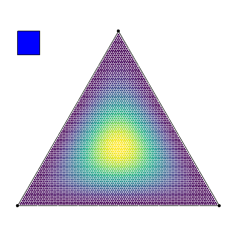
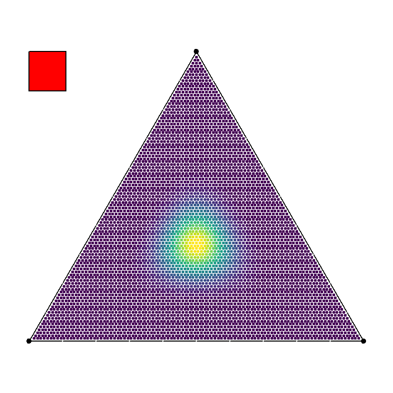
$\alpha=1.5$	$\alpha=3$	$\alpha=12$
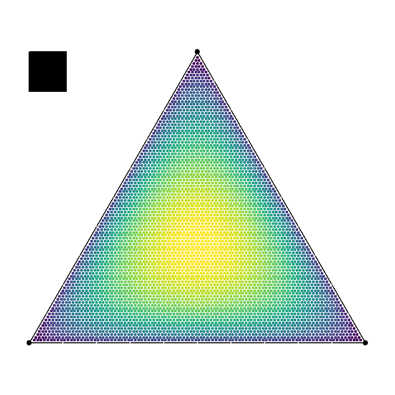
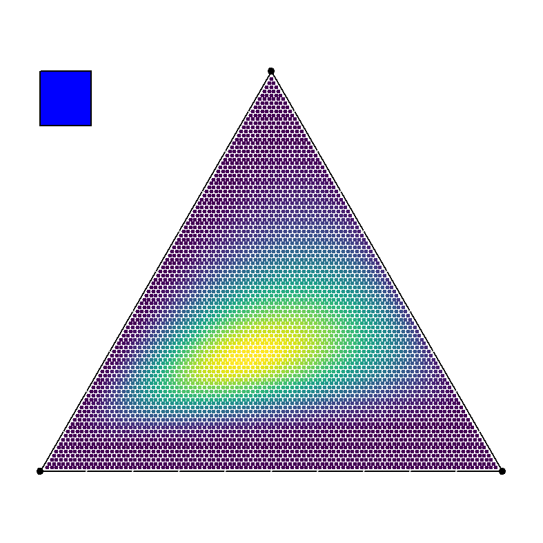
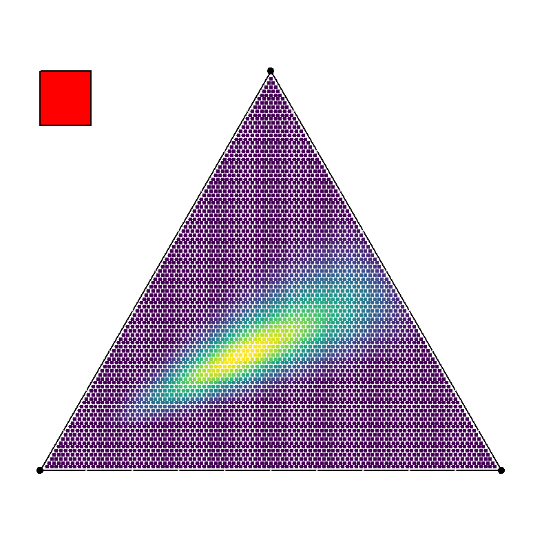
${\bm{\alpha}}=(1.5,1.5,1.5)$	${\bm{\alpha}}=(1.5,3,12)$	${\bm{\alpha}}=(1.5,12,96)$

Figure 1: Angular densities (heat maps) of the symmetric max-stable Dirichlet model (top) and of the asymmetric max-stable Dirichlet model (bottom), cf. (4) for an expression of the density. Larger values are represented by brighter colours. The corresponding max-stable distributions are stochastically ordered in the PQD sense, increasing from left to right (Theorem 4.5). The black, blue and red boxes encode the matching with Figures 6 and 7.

Second, we draw our attention to two popular parametric families of multivariate extreme value distributions that are closed under taking marginal distributions.

• Can we find order relations among the Dirichlet and Hüsler-Reiß parametric models? (Theorem 4.5 and Theorem 4.7)

The answers are affirmative. For the Hüsler-Reiß model the result may be even strengthened for the supermodular order, which is otherwise beyond the scope of this article. To give an impression of the result for the Dirichlet family, Figure 1 depicts six angular densities of the trivariate max-stable Dirichlet model. Aulbach et al. (2015) showed already that the symmetric models associated with the top row densities are decreasing in the lower orthant sense. Our new result covers the asymmetric case depicted in the bottom row; we show that the associated multivariate extreme value distributions are decreasing in the (even stronger) PQD-sense (with a more streamlined proof).

Accordingly, our text is structured as follows. Section 2 recalls some basic representations of multivariate max-stable distributions and examples of parametric models that are relevant for subsequent results. In Section 3 we review the relevant multivariate stochastic orderings together with important closure properties. This section contains also our (arguably natural) definition for corresponding order notions for exponent measures. All main results are then given in Section 4. Proofs and auxiliary results are postponed to Appendices A and B. Appendix C contains background material how we obtained the illustrations (max-zonoid envelopes for bivariate Hüsler-Reiß and Dirichlet families) depicted in Figures 2, 4, 5 and 8.

2 Prerequisites from multivariate extremes

Our main results concern stochastic orderings among max-stable distributions, or, equivalently, orderings among their respective exponent measures, cf. Theorem 4.1 below. Therefore, this section reviews some basic well-known results from the theory of multivariate extremes. Second, we will take a closer look at three marginally closed parametric families, the Dirichlet family, the Hüsler-Reiß family and the Choquet (Tawn-Molchanov) family of max-stable distributions, each model offering a different insight into phenomena of orderings among multivariate extremes.

2.1 Max-stable random vectors and their exponent measures

In order to clarify our terminology, we recall some definitions and basic facts about representations for max-stable distributions, cf. also Resnick (1987) or Beirlant et al. (2004). Operations and inequalities between vectors are meant componentwise. We abbreviate ${\bm{0}}=(0,0,\dots,0)^{\top}\in\mathbb{R}^{d}$. A random vector ${\bm{X}}=(X_{1},\dots,X_{d})^{\top}\in\mathbb{R}^{d}$ is called max-stable if for all $n\geq 1$ there exist suitable norming vectors ${\bm{a}_{n}}>{\bm{0}}$ and ${\bm{b}_{n}}\in\mathbb{R}^{d}$, such that the distributional equality

$$\max_{i=1,\dots,n}({\bm{X}_{i}})\overset{d}{=}{\bm{a}_{n}}{{\bm{X}}+{\bm{b}_{n}}}$$

holds, where ${\bm{X}_{1}},\dots,{\bm{X}_{n}}$ are i.i.d. copies of ${\bm{X}}$. According to the Fisher-Tippet theorem the marginal distributions $G_{i}(x)=\mathbb{P}(X_{i}\leq x)$ are univariate max-stable distributions, that is, either degenerate to a point mass or a generalised extreme value (GEV) distribution of the form $G_{\xi}((x-\mu)/\sigma)$ with $G_{\xi}(x)=\exp(-(1+\xi x)_{+}^{-{1}/{\xi}})$ if $\xi\neq 0$ and $G_{0}(x)=\exp(-e^{-x})$, where $\xi\in\mathbb{R}$ is a shape-parameter, while $\mu\in\mathbb{R}$ and $\sigma>0$ are the location and scale parameters, respectively. We write $\mathrm{GEV}(\mu,\sigma,\xi)$ for short.

A max-stable random vector ${\bm{X}}=(X_{1},\dots,X_{d})^{\top}$ is called simple max-stable if it has standard unit Fréchet marginals, that is, $\mathbb{P}(X_{i}\leq x)=\exp(-1/x)$, $x>0$, for all $i=1,\dots,d$. Any max-stable random vector ${\bm{X}}$ with GEV margins $X_{i}\sim\mathrm{GEV}(\mu_{i},\sigma_{i},\xi_{i})$ can be transformed into a simple max-stable random vector ${\bm{X}^{*}}$ and vice versa via the componentwise order-preserving transformations

$${X_{i}^{*}}=\Big{(}1+\xi_{i}\frac{X_{i}-\mu_{i}}{\sigma_{i}}\Big{)}^{1/\xi_{i}}\quad\text{and}\quad X_{i}=\sigma_{i}\frac{(X^{*}_{i})^{\xi_{i}}-1}{\xi_{i}}+{\mu_{i}},\quad i=1,\dots,d$$ (1)

(with the usual interpretation of $(1+\xi x)^{1/\xi}$ as $e^{x}$ for $\xi=0$). In this sense simple max-stable random vectors can be interpreted as a copula-representation for max-stable random vectors with non-degenerate margins, which encapsulates its dependence structure.

There are different ways to describe the distribution of such simple max-stable random vectors. The following will be relevant for us. Note that such vectors take values in the open upper orthant $(0,\infty)^{d}$ almost surely. Here and hereinafter we shall denote the $i$-th indicator vector by ${\bm{e}_{i}}$ (all components of ${\bm{e}_{i}}$ are zero except for the $i$-th component, which takes the value one).

Theorem/Definition 2.1 (Representations of simple max-stable distributions).

A random vector ${\bm{X}}=(X_{1},\dots,X_{d})^{\top}$ with distribution function $G({\bm{x}})=\exp(-V({\bm{x}}))$, ${\bm{x}}\in(0,\infty]^{d}$, is simple max-stable if and only if the exponent function $V$ can be represented in one of the following equivalent ways:

1. Spectral representation (de Haan, 1984). There exists a finite measure space $(\Omega,\mathcal{A},\nu)$ and a measurable function $f:\Omega\to[0,\infty)^{d}$ such that $\int_{\Omega}f_{i}({\omega})\;\nu(\mathrm{d}{\omega})=1$ for $i=1,\dots,d$, and

   $$V(x_{1},\dots,x_{d})=\int_{\Omega}\max_{i=1,\dots,d}\frac{f_{i}(\omega)}{x_{i}}\;\nu(\mathrm{d}\omega).$$

2. Exponent measure (Resnick, 1987). There exists a $(-1)$-homogeneous measure $\Lambda$ on $[0,\infty)^{d}\setminus\{{\bm{0}}\}$, such that

   $$\Lambda\Big{(}\big{\{}y\in[0,\infty)^{d}\,:\,y_{i}>1\big{\}}\Big{)}=1$$

   for $i=1,\dots,d$, and

   $$V(x_{1},x_{2},\dots,x_{d})=\Lambda\Big{(}\big{\{}y\in[0,\infty)^{d}\,:\,y_{i}>x_{i}\text{ for some }i\in\{1,\dots,d\}\big{\}}\Big{)}.$$

3. Stable tail dependence function (Ressel, 2013). There exists a $1$-homogeneous and max-completely alternating function $\ell:[0,\infty)^{d}\to[0,\infty)$, such that $\ell({\bm{e}_{i}})=1$ for $i=1,\dots,d$, and

   $$V(x_{1},\dots,x_{d})=\ell\bigg{(}\frac{1}{x_{1}},\dots,\frac{1}{x_{d}}\bigg{)}$$

   (cf. Appendix B for the notion of max-complete alternation).

In fact, the spectral representation can be seen as a polar decomposition of the exponent measure $\Lambda$, cf. e.g. Resnick (1987) or Beirlant et al. (2004). Importantly, it is not uniquely determined by the law of ${\bm{X}}$. Typical choices for the measure space $(\Omega,\mathcal{A},\nu)$ include (i) the unit interval with Lebesgue measure or (ii) a sphere $\Omega=\{{\bm{\omega}}\in[0,\infty)^{d}\;:\;\lVert{\bm{\omega}}\rVert=1\}$ with respect to some norm $\lVert\cdot\rVert$, for instance the $\ell_{p}$-norm

$$\lVert{\bm{x}}\rVert_{p}=\bigg{(}\sum_{i=1,\dots,d}\lvert x_{i}\rvert^{p}\bigg{)}^{1/p}$$

for some $p\geq 1$. For (i) it is then the spectral map $f$ which contains all dependence information. For (ii) one usually considers the component maps $f_{i}({\bm{\omega}})=\omega_{i}$, so that the measure $\nu$, then often termed angular measure, absorbs the dependence information. For a given spectral representation $(\Omega,\mathcal{A},\nu,f)$ one may rescale $\nu$ to a probability measure and absorb the rescaling constant into the spectral map $f$. The resulting random vector ${\bm{Z}}=(Z_{1},\dots,Z_{d})^{\top}$ such that $\mathbb{E}(Z_{i})={1}$, $i=1,\dots,d$, and

$$V(x_{1},\dots,x_{d})=\mathbb{E}\max_{i=1,\dots,d}\bigg{(}\frac{Z_{i}}{x_{i}}\bigg{)},$$

has been termed generator of ${\bm{X}}$, cf. Falk (2019). A useful observation is the following; for a given vector ${\bm{x}}$ with values in $\mathbb{R}^{d}$ and a subset $A\subset\{1,\dots,d\}$, let ${\bm{x}}_{A}$ be the subvector with components in $A$.

Lemma 2.2.

Let ${\bm{Z}}$ be a generator for the max-stable law ${\bm{X}}$, then ${\bm{Z}}_{A}$ is a generator for ${\bm{X}}_{A}$.

The stable tail dependence function $\ell$ goes back to Huang (1992) and has also been called D-norm (Falk et al., 2004) of ${\bm{X}}$. Since $\ell$ is 1-homogeneous, it suffices to know its values on the unit simplex $\triangle_{d}=\{{\bm{x}}\in[0,\infty)^{d}\,:\,\lVert{\bm{x}}\rVert_{1}=1\}$; the restriction of $\ell$ to $\triangle_{d}$ is called Pickands dependence function

$$A(x_{1},\dots,x_{d})=\ell(x_{1},\dots,x_{d}),\qquad(x_{1},\dots,x_{d})^{\top}\in\triangle_{d}.$$

There exist further descriptors of the dependence structure, e.g. in terms of Point processes or LePage representation, cf. e.g. Resnick (1987) or, in a very general context, Davydov et al. (2008). Copulas of max-stable random vectors on standard uniform margins are called extreme value copulas (Gudendorf and Segers, 2010).

Let us close with a representation that allows for some interesting geometric interpretations. Molchanov (2008) introduced a convex body $K\subset[0,\infty)^{d}$, which can be interpreted (up to rescaling) as selection expectation of a random cross polytope associated with the (normalised) spectral measure $\nu$. It turns out that the stable tail dependence function is in fact the support function of $K$

$$\ell({\bm{x}})=\sup\{\langle{\bm{x}},{\bm{k}}\rangle\;|\;{\bm{k}}\in K\}.$$ (2)

The convex body $K$ is called max-zonoid (or dependency set) of ${\bm{X}}$ and it is uniquely determined by the law of ${\bm{X}}$. In fact

$$K=\big{\{}{\bm{k}}\in[0,\infty)^{d}\,:\,\langle{\bm{k}},{\bm{x}}\rangle\leq\ell({\bm{x}})\text{ for all }{\bm{x}}\in[0,\infty)^{d}\big{\}}.$$ (3)

In general, it is difficult to translate one representation from Theorem 2.1 into another apart from the obvious relations

$$\ell({\bm{x}}) =\mathbb{E}\max_{i=1,\dots,d}(x_{i}Z_{i})=\int_{\Omega}\max_{i=1,\dots,d}x_{i}{f_{i}(\omega)}\;\nu(\mathrm{d}\omega)=\Lambda\Big{(}\big{\{}y\in[0,\infty)^{d}\,:\,\max_{i=1,\dots,d}(x_{i}y_{i})>1\big{\}}\Big{)}$$

for ${\bm{x}}\geq{\bm{0}}$. For convenience, we have added material in Appendix C how to obtain the boundary of a max-zonoid $K$ from the stable tail dependence function $\ell$ in the bivariate case, which will help to illustrate some of the results below.

2.2 Parametric models

Several parametric models for max-stable random vectors have been summarised for instance in Beirlant et al. (2004). In what follows we draw our attention to two of the most popular parametric models, the Dirichlet and Hüsler-Reiß families, as well as the Choquet model (Tawn-Molchanov model), which will reveal some interesting phenomena and (counter-)examples of stochastic ordering relations.

2.2.1 Dirichlet model

Coles and Tawn (1991) compute densities of angular measures of simple max-stable random vectors constructed from non-negative functions on the unit simplex $\triangle_{d}$. In particular, the following asymmetric Dirichlet model has been introduced. We summarise some equivalent characterisations, each of which may serve as a definition of the asymmetric Dirichlet model. This model has gained popularity due to its flexibility and simple structure forming the basis of Dirichlet mixture models (Boldi and Davison, 2007; Sabourin and Naveau, 2014).

Theorem/Definition 2.3 (Multivariate max-stable Dirichlet distribution).

A random vector ${\bm{X}}=(X_{1},\dots,X_{d})^{\top}$ is simple max-stable Dirichlet distributed with parameter vector ${\bm{\alpha}}=(\alpha_{1},\dots,\alpha_{d})^{\top}\in(0,\infty)^{d}$, we write

$${\bm{X}}=(X_{1},\dots,X_{d})^{\top}\leavevmode\nobreak\ \sim\mathrm{MaxDir}(\alpha_{1},\dots,\alpha_{d})=\mathrm{MaxDir}({\bm{\alpha}})$$

for short, if and only if one of the following equivalent conditions is satisfied:

1. (Gamma generator) A generator of ${\bm{X}}$ is the random vector

   $${\bm{\alpha}}^{-1}{\bm{\Gamma}}=(\Gamma_{1}/\alpha_{1},\Gamma_{2}/\alpha_{2},\dots,\Gamma_{d}/\alpha_{d})^{\top},$$

   where ${\bm{\Gamma}}=(\Gamma_{1},\dots,\Gamma_{d})^{\top}$ consists of independent Gamma distributed variables $\Gamma_{i}\sim\Gamma(\alpha_{i})$, $\alpha_{i}>0$, $i=1,\dots,d$. Here, the Gamma distribution $\Gamma(\alpha_{i})$ has the density

   $$\gamma_{\alpha_{i}}(x)=\frac{x^{\alpha_{i}-1}}{\Gamma(\alpha_{i})}\exp\big{(}-{x}\big{)}.$$

2. (Dirichlet generator) A generator of ${\bm{X}}$ is the random vector

   $$({\bm{\alpha}}^{-1}\lVert{\bm{\alpha}}\rVert_{1}){\bm{D}}=(\alpha_{1}+\dots+\alpha_{d})\cdot(D_{1}/\alpha_{1},D_{2}/\alpha_{2},\dots,D_{d}/\alpha_{d})^{\top},$$

   where ${\bm{D}}$ follows a Dirichlet distribution $\mathrm{Dir}(\alpha_{1},\dots,\alpha_{d})$ on the unit simplex $\triangle_{d}$ with density

   $$d({\omega_{1},\dots,\omega_{d}})=\Gamma(\lVert{\bm{\alpha}}\rVert_{1})\prod_{i=1}^{d}\frac{\omega_{i}^{\alpha_{i}-1}}{\Gamma(\alpha_{i})},\quad(\omega_{1},\dots,\omega_{d})^{\top}\in\triangle_{d}.$$

3. (Angular measure) The density of the angular measure of ${\bm{X}}$ on $\triangle_{d}$ is given by

   $$h(\omega_{1},\dots,\omega_{d})=\frac{\Gamma(\lVert{\bm{\alpha}}\rVert_{1}+1)}{\lVert{\bm{\alpha}}{\bm{\omega}}\rVert_{1}}\prod_{i=1}^{d}\frac{\alpha_{i}^{\alpha_{i}}\omega_{i}^{\alpha_{i}-1}}{\Gamma(\alpha_{i})(\lVert{\bm{\alpha}}{\bm{\omega}}\rVert_{1})^{\alpha_{i}}},\quad(\omega_{1},\dots,\omega_{d})^{\top}\in\triangle_{d}.$$ (4)

To the best of our knowledge the representation through the Gamma generator, albeit inspired by Aulbach et al. (2015) from the fully symmetric case, is new in this generality. We have added a proof in Appendix A.2. An advantage of the representation with the Gamma generator is that it reveals immediately the closure of the model with respect to taking marginal distributions, cf. Lemma 2.2, a result that has been previously obtained in Ballani and Schlather (2011), but with a one-page proof and some intricate density calculations.

Lemma 2.4 (Closure of Dirichlet model under taking marginals).

Let ${\bm{X}}=(X_{1},\dots,X_{d})^{\top}\sim\mathrm{MaxDir}(\alpha_{1},\dots,\alpha_{d})=\mathrm{MaxDir}({\bm{\alpha}})$ and $A\subset\{1,\dots,d\}$, then ${\bm{X}}_{A}\sim\mathrm{MaxDir}({\bm{\alpha}}_{A})$.

The angular density representation on the other hand is useful to see that different parameter vectors ${\bm{\alpha}}\neq{\bm{\beta}}$ lead in fact to different multivariate distributions $\mathrm{MaxDir}({\bm{\alpha}})\neq\mathrm{MaxDir}({\bm{\beta}})$ for $d\geq 2$, so that $(0,\infty)^{d}$ is indeed the natural parameter space for this model.

2.2.2 Hüsler-Reiß model

The multivariate Hüsler-Reiß distribution (Hüsler and Reiß, 1989) forms the basis of the popular Brown-Resnick process (Kabluchko et al., 2009) and has sparked significant interest from the perspectives of spatial modelling (Davison et al., 2019) and more recently in connection with graphical modelling of extremes (Engelke and Hitz, 2020). The natural parameter space for this model is the convex cone of conditionally negative symmetric $d\times d$-matrices, whose diagonal entries are zero

$$\mathcal{G}_{d}=\bigg{\{}{\bm{\gamma}}=(\gamma_{ij})_{i,j\in\{1,\dots,d\}}\in\mathbb{R}^{d\times d}\,:\,\begin{array}[]{c}\gamma_{ij}=\gamma_{ji},\,\gamma_{ii}=0\text{ for all $i,j\in\{1,\dots,d\}$, }\\ v^{\top}{\bm{\gamma}}v\leq 0\text{ for all }v\in\mathbb{R}^{d}\text{ such that }v_{1}+\dots+v_{d}=0\end{array}\bigg{\}}.$$

It is well-known, cf. e.g. Berg et al. (1984, Ch. 3), that for a given ${\bm{\gamma}}\in\mathcal{G}_{d}$, there exists a zero mean Gaussian random vector ${\bm{W}}=(W_{1},\dots,W_{d})^{\top}$ with incremental variance

$$\mathbb{E}(W_{i}-W_{j})^{2}=\gamma_{ij},\qquad i,j\in\{1,\dots,d\},$$ (5)

although its distribution is not uniquely specified by this condition. For instance, select $i\in\{1,\dots,d\}$. Imposing additionally the linear constraint “$W_{i}=0$ almost surely” leads to ${\bm{W}}\sim\mathcal{N}({\bm{0}},{\bm{\Sigma}_{i}})$ with

$$({\bm{\Sigma}_{i}})_{jk}=\frac{1}{2}\big{(}\gamma_{ij}+\gamma_{ik}-\gamma_{jk}\big{)},\qquad j,k\in\{1,\dots,d\},$$

which satisfies (5).

Theorem/Definition 2.5 (Multivariate Hüsler-Reiss distribution, cf. Kabluchko (2011) Theorem 1).

Let ${\bm{\gamma}}\in\mathcal{G}_{d}$ and (5) be valid. Consider the simple max-stable random vector ${\bm{X}}=(X_{1},\dots,X_{d})^{\top}$ defined by the generator ${\bm{Z}}=(Z_{1},\dots,Z_{d})^{\top}$ with

$$Z_{i}=\exp\bigg{(}W_{i}-\frac{1}{2}\mathrm{Var}(W_{i})\bigg{)},\qquad i=1,\dots,d.$$

Then the distribution of ${\bm{X}}$ depends only on ${\bm{\gamma}}$ and not on the specific choice of a zero mean Gaussian distribution satisfying (5). We call ${\bm{X}}$ simple Hüsler-Reiß distributed with parameter matrix ${\bm{\gamma}}$ and write for short

$${\bm{X}}=(X_{1},\dots,X_{d})^{\top}\leavevmode\nobreak\ \sim\mathrm{HR}({\bm{\gamma}}).$$

We also note that for ${\bm{\gamma}}_{1},\,{\bm{\gamma}}_{2}\in\mathcal{G}_{d}$, the distributions $\mathrm{HR}({\bm{\gamma}}_{1})$ and $\mathrm{HR}({\bm{\gamma}}_{2})$ coincide if and only if ${\bm{\gamma}}_{1}={\bm{\gamma}}_{2}$, so that $\mathcal{G}_{d}$ is indeed the natural parameter space for these models. This follows directly from the observation that the multivariate Hüsler-Reiß model is also closed under taking marginal distributions and the equivalent statement for bivariate Hüsler-Reiß models, which can be seen for instance from (19) below. Indeed, we also state the following lemma for clarity. It follows directly from the generator representation of $\mathrm{HR}({\bm{\gamma}})$ and Lemma 2.2.

Lemma 2.6 (Closure of Hüsler-Reiß model under taking marginals).

Let ${\bm{X}}=(X_{1},\dots,X_{d})^{\top}\sim\mathrm{HR}({\bm{\gamma}})$ and $A\subset\{1,\dots,d\}$, then ${\bm{X}}_{A}\sim\mathrm{HR}({\bm{\gamma}}_{A\times A})$, where ${\bm{\gamma}}_{A\times A}$ is the restriction of ${\bm{\gamma}}$ to the components of $A$ in both rows and columns.

It is well-known that up to a change of location and scale parameters Hüsler-Reiß distributions are the only possible limit laws of maxima of triangular arrays of multivariate Gaussian distributions, a finding which can be traced back to Hüsler and Reiß (1989) and Brown and Resnick (1977). The following version will be convenient for us.

Theorem 2.7 (Triangular array convergence of maxima of Gaussian vectors, cf. Kabluchko (2011) Theorem 2).

Let $u_{n}$ be a sequence such that $\sqrt{2\pi}u_{n}e^{u_{n}^{2}/2}/n\to 1$ as $n\to\infty$. For each $n\in\mathbb{N}$ let ${\bm{Y}^{(n)}_{1}},{\bm{Y}^{(n)}_{2}},\dots,{\bm{Y}^{(n)}_{n}}$ be independent copies of a $d$-variate zero mean unit-variance Gaussian random vector with correlation matrix $(\rho^{(n)}_{ij})_{i,j\in\{1,\dots,d\}}$. Suppose that for all $i,j\in\{1,\dots,d\}$

$$4\log(n)(1-\rho^{(n)}_{ij})\to\gamma_{ij}\in[0,\infty)$$

as $n\to\infty$. Then the matrix ${\bm{\gamma}}=(\gamma_{ij})_{i,j\in\{1,\dots,d\}}$ is necessarily and element of $\mathcal{G}_{d}$. Let ${\bm{M}}^{(n)}$ be the componentwise maximum of ${\bm{Y}^{(n)}_{1}},{\bm{Y}^{(n)}_{2}},\dots,{\bm{Y}^{(n)}_{n}}$. Then the componentwise rescaled vector $u_{n}({\bm{M}}^{(n)}-u_{n})$ converges in distribution to the Hüsler-Reiß distribution $\mathrm{HR}({\bm{\gamma}})$.

Remark 2.8.

In the bivariate case we have $\gamma_{12}=\gamma_{21}=\gamma\in[0,\infty)$ and the boundary case $\gamma=0$ leads to a degenerate random vector with fully dependent components, whereas $\gamma\uparrow\infty$ leads to a random vector with independent components. More generally, one might also admit the value $\infty$ for $\gamma_{ij}$ in the multivariate case, as long as the resulting matrix ${\bm{\gamma}}$ is negative definite in the extended sense, cf. Kabluchko (2011). This extension corresponds to a partition of ${\bm{X}}$ into independent subvectors ${\bm{X}}=\bigsqcup_{A}{\bm{X}}_{A}$, where each ${\bm{X}}_{A}$ is a Hüsler-Reiß random vector in the usual sense. Here $\gamma_{ij}=\infty$ precisely when $i$ and $j$ are in different subsets of the partition. Theorem 2.7 extends to this situation as well. In fact, is has been formulated in this generality in Kabluchko (2011).

2.2.3 Choquet model / Tawn-Molchanov model

A popular way to summarise extremal dependence information within a random vector is by considering its extremal coefficients, which in the case of a simple max-stable random vector ${\bm{X}}=(X_{1},X_{2},\dots,X_{d})^{\top}$ may be expressed as

$$\theta(A)=\ell({\bm{e}}_{A}),\qquad{\bm{e}}_{A}=\sum_{i\in A}{\bm{e}}_{i},\qquad A\subset\{1,\dots,d\},\,A\neq\emptyset,$$

or, equivalently,

$$\theta(A)=\mathbb{E}\max_{i\in A}Z_{i}=\int_{\Omega}\max_{i\in A}{f_{i}(\omega)}\;\nu(\mathrm{d}\omega)=\Lambda\Big{(}\big{\{}y\in[0,\infty)^{d}\,:\,\max_{i\in A}(y_{i})>1\big{\}}\Big{)},$$ (6)

where $\ell$ is the stable tail dependence function, ${\bm{Z}}$ a generator, $\Lambda$ the exponent measure and $(\Omega,\mathcal{A},\nu,f)$ a spectral representation for ${\bm{X}}$. Loosely speaking, the coefficient $\theta(A)$, which takes values in $[1,|A|]$, can be interpreted as the effective number of independent variables among the collection $(X_{i})_{i\in A}$. We have $\theta(\{i\})=1$ for singletons $\{i\}$ and naturally $\theta(\emptyset)=0$.

The following result can be traced back to Schlather and Tawn (2002) and Molchanov (2008). Accordingly, the associated max-stable model, which can be parametrised by its extremal coefficients, has been introduced as Tawn-Molchanov model in Strokorb and Schlather (2015). It is essentially an application of the the Choquet theorem (see Molchanov (2017) Section 1.2 and Berg et al. (1984) Theorem 6.6.19), which also holds for not necessarily finite capacities (see Schneider and Weil (2008) Theorem 2.3.2). Therefore, it has been relabelled Choquet model in Molchanov and Strokorb (2016), cf. Appendix B for background on complete alternation. We write $\mathcal{P}_{d}$ for the power set of $\{1,\dots,d\}$ henceforth.

Theorem 2.9.

1. Let $\theta:\mathcal{P}_{d}\to\mathbb{R}$. Then $\theta$ is the extremal coefficient function of a simple max-stable random vector in $(0,\infty)^{d}$ if and only if $\theta(\emptyset)=0$, $\theta(\{i\})=1$ for all $i=1,\dots,d$ and $\theta$ is union-completely alternating.

2. Let $\theta:\mathcal{P}_{d}\to\mathbb{R}$ be an extremal coefficient function. Let

   $$\ell^{*}({\bm{x}})=\int_{0}^{\infty}\theta(\{i\,:\,x_{i}\geq t\})\,dt,\quad{\bm{x}}\in[0,\infty)^{d}$$

   be the Choquet integral with respect to $\theta$. Then $\ell^{*}$ is a valid stable tail dependence function, which retrieves the given extremal coefficients $\ell^{*}({\bm{e}}_{A})=\theta(A)$ for all $A\in\mathcal{P}_{d}$. Its max-zonoid is given by

   $$K^{*}=\big{\{}{\bm{k}}\in[0,\infty)^{d}\,:\,\langle{\bm{k}},{\bm{e}}_{A}\rangle\leq\theta(A)\text{ for all }A\in\mathcal{P}_{d}\big{\}}.$$

3. Let $\ell$ be any stable tail dependence function with extremal coefficient function $\theta$ and $K$ its corresponding max-zonoid. Then

   $$\ell({\bm{x}})\leq\ell^{*}({\bm{x}}),\quad{\bm{x}}\geq 0\qquad\text{and}\qquad K\subset K^{*}.$$

Example 2.10 (Choquet model in the bivariate case).

Let $\ell$ be a bivariate stable tail dependence function and $\theta=\ell(1,1)\in[1,2]$ the bivariate extremal coefficient. Then the associated Choquet model is given by the max-zonoid $K^{*}=\{(x_{1},x_{2})\in[0,1]^{2}\,:\,x_{1}+x_{2}\leq\theta\}$ or the stable tail dependence function $\ell^{*}(x_{1},x_{2})=\max(x_{1}+(\theta-1)x_{2},(\theta-1)x_{1}+x_{2})$. Figure 2 displays a situation, where the original $\ell$ stems from an asymmetric Dirichlet model.

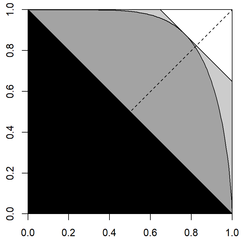
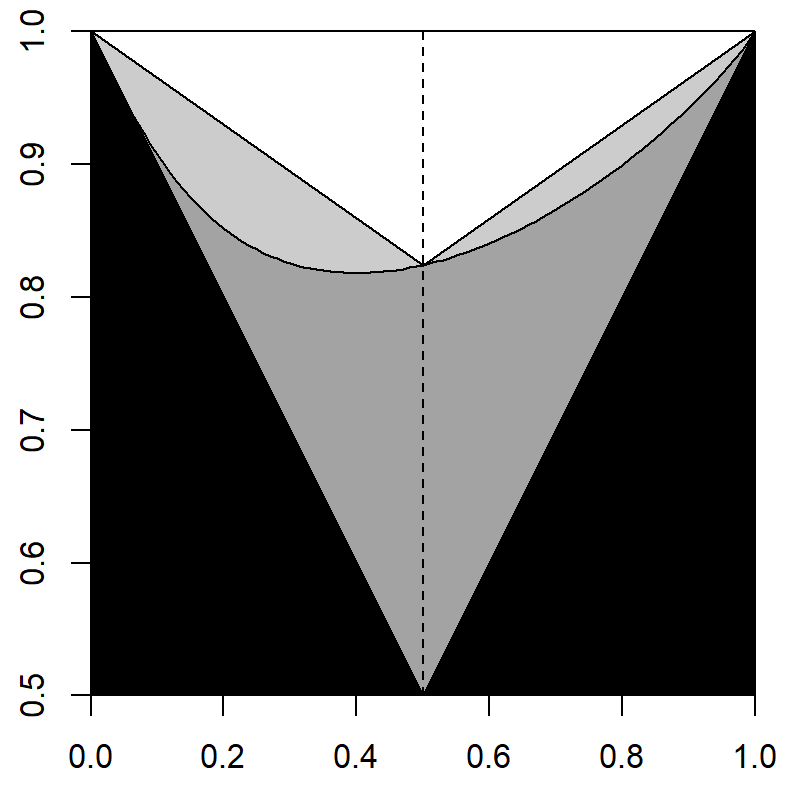
Figure 2: Nested max-zonoids and Pickands dependence functions ranging from full dependence (black), an asymmetric Dirichlet model with ${\bm{\alpha}}=(30,0.2)$ (dark grey), its associated Choquet (Tawn-Molchanov) model (light grey) to the fully independent model (white).

In geometric terms, for any given max-zonoid $K\subset[0,1]^{d}$ the associated Choquet max-zonoid $K^{*}\subset[0,1]^{d}$ is bounded by $2^{d}-1$ hyperplanes, one for each direction ${\bm{e}}_{A}$, which is the supporting hyperplane of the max-zonoid $K$ in the direction of ${\bm{e}}_{A}$.

The Choquet model is a spectrally discrete max-stable model, whose exponent measure has its support contained in the rays through the vectors ${\bm{e}}_{A}$, $A\subset\{1,\dots,d\}$, $A\neq\emptyset$. While its natural parameter space is the set of extremal coefficients, we can also describe it via the mass that the model puts on those rays. To this end, let $\tau:\mathcal{P}_{d}\setminus\{\emptyset\}\to\mathbb{R}$ be given as follows

$$\tau(A) =-(\Delta_{a_{1}}\Delta_{a_{2}}\dots\Delta_{a_{n}}\theta)(\{1,\dots,d\}\setminus A)=\sum_{I\subset A}(-1)^{|I|+1}\theta(I\cup(\{1,\dots,d\}\setminus A)),$$

where we assume $a_{1},a_{2},\dots,a_{n}$ to be the distinct elements from $A\subset\{1,\dots,d\}$. Then the spectral representation $(\Omega,\mathcal{A},\nu^{*},f)$ with $\Omega=\{{\bm{\omega}}\in[0,\infty)^{2}\,:\,\lVert{\bm{\omega}}\rVert_{\infty}=1\}$, $f_{i}({\bm{\omega}})=\omega_{i}$ and

$$\nu^{*}=\sum_{A\in\mathcal{P}_{d}\setminus\{\emptyset\}}\tau(A)\,\delta_{{\bm{e}}_{A}}$$ (7)

corresponds to the stable tail dependence function $\ell^{*}$ from Theorem 2.9. In terms of an underlying generator for which (6) holds true, we may express $\tau$ as

$$\tau(A)=\mathbb{E}\Big{(}\min_{i\in A}Z_{i}-\max_{i\in\{1,\dots,d\}\setminus A}Z_{i}\Big{)}_{+},$$

cf. Papastathopoulos and Strokorb (2016) Lemma 3. Moreover, we recover $\theta$ from $\tau$ via

$$\theta(A)=\sum_{K\,:\,K\cap A\neq\emptyset}\tau(K),$$

which makes the analogy between extremal coefficient functions $\theta$ and capacity functionals of random sets even more explicit.

However, there are two drawbacks with representing the Choquet model by the collection of coefficients $\tau(A)$, $A\subset\{1,\dots,d\}$, $A\neq\emptyset$. First, this representation is specific to the dimension, in which the model is considered, that is, we cannot simply turn to a subset of these coefficients when considering marginal distributions. Second, one may easily forget that one has in fact not $2^{d}-1$ degrees of freedom among these coefficients, but $2^{d}-1-d$, since $\theta(\{i\})=1$ for singletons $\{i\}$, which is only encoded through $d$ linear constraints for $\tau$ as follows

$$\sum_{K\,:\,i\in K}\tau(K)=1,\qquad i=1,\dots,d.$$ (8)

A third parametrisation of the Choquet model, which has received little attention so far, but is very relevant for the ordering results in this article (cf. Lemma 4.12) and does not have such drawbacks, is the following. Instead of extremal coefficients, let us consider the following tail dependence coefficients for $A\subset\{1,\dots,d\}$, $A\neq\emptyset$:

$$\chi(A)=\mathbb{E}\min_{i\in A}Z_{i}=\int_{\Omega}\min_{i\in A}{f_{i}(\omega)}\;\nu(\mathrm{d}\omega)=\Lambda\Big{(}\big{\{}y\in[0,\infty)^{d}\,:\,\min_{i\in A}(y_{i})>1\big{\}}\Big{)}.$$

Then it is easily seen that

$$\chi(A)=\sum_{I\subset A,\,I\neq\emptyset}(-1)^{|I|+1}\theta(I)\qquad\text{and}\qquad\theta(A)=\sum_{I\subset A,\,I\neq\emptyset}(-1)^{|I|+1}\chi(I).$$ (9)

Since $\theta(\emptyset)=0$, and with $a_{1},\dots,a_{n}$ being the distinct elements of $A$, the first identity may also be expressed as

$$\chi(A)=-(\Delta_{a_{1}}\Delta_{a_{2}}\dots\Delta_{a_{n}}\theta)(\emptyset).$$ (10)

In particular $\chi(\{i\})=\theta(\{i\})=1$ for $i=1,\dots,d$, and these operations show explicitly, how $\theta$ and $\chi$ can be recovered from each other. While $\theta$ resembles a capacity functional, $\chi$ can be seen as an analog of an inclusion functional, since

$$\chi(A)=\sum_{K\,:\,A\subset K}\tau(K),$$ (11)

whereas

$$\tau(A)=\sum_{K\,:\,A\subset K}(-1)^{|K\setminus A|}\chi(K)=(\Delta_{b_{1}}\Delta_{b_{2}}\dots\Delta_{b_{m}}\chi)(A),$$

where $b_{1},b_{2},\dots,b_{m}$ are the distinct elements of $\{1,2,\dots,d\}\setminus A$.

To sum up, we may consider three different parametrizations for the Choquet model:

1. by the $2^{d}-1$ extremal coefficients $\theta(A)$, $A\in\mathcal{P}_{d}$, $A\neq\emptyset$,

2. by the $2^{d}-1$ tail dependence coefficients $\chi(A)$, $A\in\mathcal{P}_{d}$, $A\neq\emptyset$,

3. by the $2^{d}-1$ mass coefficients $\tau(A)$, $A\in\mathcal{P}_{d}$, $A\neq\emptyset$.

For (i) and (ii) the constraint for standard unit Fréchet margins is encoded via $\chi(\{i\})=\theta(\{i\})=1$ for $i=1,\dots,d$. For (iii) it amounts to the $d$ conditions from (8). Only (i) and (ii) do not depend on the dimension, in which the model is considered.

3 Prerequisites from stochastic orderings

A wealth of stochastic orderings and associated inequalities have been summarised in Müller and Stoyan (2002) and Shaked and Shanthikumar (2007), the most fundamental order being the usual stochastic order

$$F\leq_{\mathrm{st}}G$$

between two univariate distributions $F$ and $G$, which is defined as $F(x)\geq G(x)$ for all $x\in\mathbb{R}$. This means that draws from $F$ are less likely to attain large values than draws from $G$.

For multivariate distributions definitions of orderings are less straightforward and there are many more notions of stochastic orderings. We will focus on upper orthants, lower orthants and the PQD order here. A subset $U\subset\mathbb{R}^{d}$ is called an upper orthant if it is of the form

$$U=U_{{\bm{a}}}=\{{\bm{x}}\in\mathbb{R}^{d}\,:\,x_{1}>a_{1},\dots,x_{d}>a_{d}\}$$

for some ${\bm{a}}\in\mathbb{R}^{d}$. Similarly, a subset $L\subset\mathbb{R}^{d}$ is called a lower orthant if it is of the form

$$L=L_{{\bm{a}}}=\{{\bm{x}}\in\mathbb{R}^{d}\,:\,x_{1}\leq a_{1},\dots,x_{d}\leq a_{d}\}$$

for some ${\bm{a}}\in\mathbb{R}^{d}$.

Definition 3.1 (Multivariate orders LO, UO, PQD, Shaked and Shanthikumar (2007), Sections 6.G and 9.A, Müller and Stoyan (2002), Sections 3.3. and 3.8).

  
Let ${\bm{X}},{\bm{Y}}\in\mathbb{R}^{d}$ be two random vectors.

• ${\bm{X}}$ is said to be smaller than ${\bm{Y}}$ in the upper orthant order, denoted ${\bm{X}}\leq_{\mathrm{uo}}{\bm{Y}}$,
  if $\mathbb{P}({\bm{X}}\in U)\leq\mathbb{P}({\bm{Y}}\in U)$ for all upper orthants $U\subset\mathbb{R}^{d}$.

• ${\bm{X}}$ is said to be smaller than ${\bm{Y}}$ in the lower orthant order, denoted ${\bm{X}}\leq_{\mathrm{lo}}{\bm{Y}}$,
  if $\mathbb{P}({\bm{X}}\in L)\geq\mathbb{P}({\bm{Y}}\in L)$ for all lower orthants $L\subset\mathbb{R}^{d}$.

• ${\bm{X}}$ is said to be smaller than ${\bm{Y}}$ in the positive quadrant order , denoted ${\bm{X}}\leq_{\mathrm{PQD}}{\bm{Y}}$,
  if we have the relations ${\bm{X}}\leq_{\mathrm{uo}}{\bm{Y}}$ and ${\bm{X}}\geq_{\mathrm{lo}}{\bm{Y}}$.

Note that the PQD order (also termed concordance order) is a dependence order. If ${\bm{X}}\leq_{\mathrm{PQD}}{\bm{Y}}$ holds, it implies that ${\bm{X}}$ and ${\bm{Y}}$ have identical univariate marginals. Several equivalent characterizations of these orders are summarised in the respective sections of Müller and Stoyan (2002) and Shaked and Shanthikumar (2007). In relation to portfolio properties, it is interesting to note that for non-negative random vectors ${\bm{X}},{\bm{Y}}\in[0,\infty)^{d}$

$${\bm{X}}\leq_{\mathrm{uo}}{\bm{Y}}\quad\iff\quad\min_{i=1,\dots,d}(a_{i}X_{i})\leq_{\mathrm{st}}\min_{i=1,\dots,d}(a_{i}Y_{i})\quad\text{ for all }{\bm{a}}\in(0,\infty)^{d};$$ (12)

$${\bm{X}}\leq_{\mathrm{lo}}{\bm{Y}}\quad\iff\quad\max_{i=1,\dots,d}(a_{i}X_{i})\leq_{\mathrm{st}}\max_{i=1,\dots,d}(a_{i}Y_{i})\quad\text{ for all }{\bm{a}}\in(0,\infty)^{d}.$$ (13)

In addition, if ${\bm{X}},{\bm{Y}}\in[0,\infty)^{d}$ and ${\bm{X}}\leq_{\mathrm{lo}}{\bm{Y}}$, then

$$\mathbb{E}\,g\bigg{(}\sum_{i=1}^{d}a_{i}X_{i}\bigg{)}\leq\mathbb{E}\,g\bigg{(}\sum_{i=1}^{d}a_{i}Y_{i}\bigg{)},$$

for all ${\bm{a}}\in[0,\infty)^{d}$ and all Bernstein functions $g$, provided that the expectation exists, cf. Shaked and Shanthikumar (2007) 6.G.14 and 5.A.4 for this fact and Appendix B for a definition of Bernstein functions. In particular, such functions are non-negative, monotonously increasing and concave and therefore form a natural class of utility functions, see e.g. Brockett and Golden (1987) and Caballé and Pomansky (1996). Important examples of Bernstein functions include the identity function, $g(x)=\log(1+x)$ or $g(x)=(1+x)^{\alpha}-1$ for $\alpha\in(0,1)$.

The multivariate orders from Definition 3.1 have several useful closure properties. We refer to Müller and Stoyan (2002) Theorem 3.3.19 and Theorem 3.8.7 for a systematic collection, including

• independent or identical concatenation,

• marginalisation,

• distributional convergence,

• applying increasing transformations to the components,

• taking mixtures.

In what follows, we will need a corresponding notion of multivariate orders not only for probability measures on $\mathbb{R}^{d}$, but also for exponent measures as introduced in Section 2. While the support of an exponent measure $\Lambda$ is contained in $[0,\infty)^{d}\setminus\{{\bm{0}}\}$, its total mass is infinite. We only know for sure that $\Lambda(B)$ is finite for Borel sets $B\subset\mathbb{R}^{d}$ bounded away from the origin in the sense that there exists $\varepsilon>0$, such that $B\cap L_{\varepsilon{\bm{e}}}\neq\emptyset$ (recall $L_{\varepsilon{\bm{e}}}=\{{\bm{x}}\in\mathbb{R}^{d}\,:\,x_{1}\leq\varepsilon,\dots,x_{d}\leq\varepsilon\}$). This means that we need to assume a different view on lower orthants and work with their complements instead, a subtlety, which did not matter previously when defining such notions for probability measures only. The following notion seems natural in view of Definition 3.1 and the results of Section 4. Figure 3 illustrates the restriction to fewer admissible test sets for these orders for exponent measures.

Figure 3: Illustration of test sets for multivariate orders for exponent measures in dimension $d=2$, cf. Definition 3.2. Left: $\Lambda$ is locally finite on the (closed) grey area for all $\varepsilon>0$, its total (infinite) mass is contained in the union of such sets; middle: admissible complement of a lower orthant $\mathbb{R}^{2}\setminus L_{\bm{a}}$ (blue area) for testing lower orthant order for $\Lambda$; right: admissible upper orthants $U_{\bm{a}}$, $U_{\bm{b}}$, $U_{\bm{c}}$ (three red areas) for testing upper orthant order for $\Lambda$.

Definition 3.2 (Multivariate orders for exponent measures).

Let $\Lambda,\widetilde{\Lambda}$ be two infinite measures on $\mathbb{R}^{d}$ with mass contained in $[0,\infty)^{d}\setminus\{{\bm{0}}\}$ and taking finite values on Borel sets bounded away from the origin.

• $\Lambda$ is said to be smaller than $\widetilde{\Lambda}$ in the upper orthant order, denoted $\Lambda\leq_{\mathrm{uo}}\widetilde{\Lambda}$,
  if $\Lambda(U)\leq\widetilde{\Lambda}(U)$ for each upper orthant $U\subset\mathbb{R}^{d}$ that is bounded away from the origin.

• $\Lambda$ is said to be smaller than $\widetilde{\Lambda}$ in the lower orthant order, denoted $\Lambda\leq_{\mathrm{lo}}\widetilde{\Lambda}$,
  if $\Lambda(\mathbb{R}^{d}\setminus L)\leq\widetilde{\Lambda}(\mathbb{R}^{d}\setminus L)$ for all lower orthants $L\subset\mathbb{R}^{d}$ such that $\mathbb{R}^{d}\setminus L$ is bounded away from the origin.

• $\Lambda$ is said to be smaller than $\widetilde{\Lambda}$ in the positive quadrant order, denoted $\Lambda\leq_{\mathrm{PQD}}\widetilde{\Lambda}$,
  if we have the relations $\Lambda\leq_{\mathrm{uo}}\widetilde{\Lambda}$ and $\Lambda\geq_{\mathrm{lo}}\widetilde{\Lambda}$.

4 Main results

First we present some fundamental characterisations of LO, UO and PQD order among simple max-stable distributions and their exponent measures, then we study these orders among the introduced parametric families. While we focus on simple max-stable distributions in what follows, we would like to stress that applying componentwise identical isotonic transformations to random vectors preserves orthant and concordance orders; in this sense the following properties can be seen as statements about the respective copulas. In particular, among max-stable random vectors, it suffices to establish these orders among simple max-stable random vectors and they translate immediately to all counterparts with different marginal distributions, cf. (1).

4.1 Fundamental results

We start by assembling the most fundamental relations for multivariate orders among simple max-stable random vectors. While the statements about lower orthant orders are almost immediate from existing theory and definitions, the relations for upper orthants are a bit more intricate and non-standard in the area. In particular, showing that “$\Lambda\leq_{\mathrm{uo}}\widetilde{\Lambda}$ implies $G\leq_{\mathrm{uo}}\widetilde{G}$” turns out to be non-trivial. The key ingredient in the proof of the following theorem (cf. Appendix A.1) is Proposition B.9 for part b).

Theorem 4.1 (Orthant orders characterisations).

Let $G$ and $\widetilde{G}$ be $d$-variate simple max-stable distributions with exponent measures $\Lambda$ and $\widetilde{\Lambda}$, generators ${\bm{Z}}$ and $\widetilde{\bm{Z}}$, stable tail dependence functions $\ell$ and $\widetilde{\ell}$ and max-zonoids $K$ and $\widetilde{K}$, respectively.

1. The following statements are equivalent.

   1. $G\leq_{\mathrm{lo}}\widetilde{G}$;

   2. $\Lambda\leq_{\mathrm{lo}}\widetilde{\Lambda}$;

   3. $\mathbb{E}(\max_{i=1,\dots,d}(a_{i}Z_{i}))\leq\mathbb{E}(\max_{i=1,\dots,d}(a_{i}\widetilde{Z}_{i}))$ for all ${\bm{a}}\in(0,\infty)^{d}$;

   4. $\ell\leq\widetilde{\ell}$;

   5. $K\subset\widetilde{K}$.

2. The following statements are equivalent.

   1. $G\leq_{\mathrm{uo}}\widetilde{G}$;

   2. $\Lambda\leq_{\mathrm{uo}}\widetilde{\Lambda}$;

   3. $\mathbb{E}(\min_{i\in A}(a_{i}Z_{i}))\leq\mathbb{E}(\min_{i\in A}(a_{i}\widetilde{Z}_{i}))$ for all ${\bm{a}}\in(0,\infty)^{d}$ and $A\subset\{1,\dots,d\}$, $A\neq\emptyset$.

3. If $d=2$, the following statements are equivalent.

   1. $G\leq_{\mathrm{PQD}}\widetilde{G}$;

   2. $G\leq_{\mathrm{uo}}\widetilde{G}$;

   3. $G\geq_{\mathrm{lo}}\widetilde{G}$.

The assumption $d=2$ is important in part c); these equivalences are no longer true in higher dimensions, cf. Example 4.13 below. Theorem 4.1 implies further that the orthant ordering of two generators ${\bm{Z}}$ and ${\widetilde{\bm{Z}}}$ implies the respective ordering of the corresponding distributions ${G}$ and ${\widetilde{G}}$ and exponent measures ${\Lambda}$ and ${\widetilde{\Lambda}}$. However, the converse is false and most generators will not satisfy orthant orderings, even when the corresponding distributions do. An interesting case for this phenomenon is the Hüsler-Reiß family, cf. Example 4.11 below. The following corollary is another immediate consequence of Theorem 4.1.

Corollary 4.2 (PQD/concordance order characterisation).

Let $G$ and $\widetilde{G}$ be $d$-variate simple max-stable distributions with exponent measures $\Lambda$ and $\widetilde{\Lambda}$, then

$$G\leq_{\mathrm{PQD}}\widetilde{G}\quad\iff\quad\Lambda\leq_{\mathrm{PQD}}\widetilde{\Lambda}.$$

It is well-known that for any stable tail dependence function $\ell$ of a simple max-stable random vector

$$\ell_{\mathrm{dep}}({\bm{x}})=\lVert{{\bm{x}}}\rVert_{\infty}\leq\ell({\bm{x}})\leq\lVert{{\bm{x}}}\rVert_{1}=\ell_{\mathrm{indep}}({\bm{x}}),\qquad{\bm{x}}\geq{\bm{0}},$$ (14)

where $\ell_{\mathrm{dep}}$ represents the degenerate max-stable random vector, whose components are fully dependent, and $\ell_{\mathrm{indep}}$ corresponds to the max-stable random vector with completely independent components. From the perspective of stochastic orderings this means that every max-stable random vector is dominated by the fully independent model, while it dominates the fully dependent model with respect to the lower orthant order. It seems less well-known that the converse ordering holds true for upper orthants, so that we arrive at the following corollary.

Corollary 4.3 (PQD/concordance for independent and fully dependent model).

Let $G_{\mathrm{indep}}$, $G_{\mathrm{dep}}$ and $G$ be $d$-dimensional simple max-stable distributions, where $G_{\mathrm{indep}}$ represents the model with fully independent components, and $G_{\mathrm{dep}}$ represents the model with fully dependent components. Then

$$G_{\mathrm{indep}}\,\leq_{\mathrm{PQD}}\,G\,\leq_{\mathrm{PQD}}\,G_{\mathrm{dep}}.$$

Similarly Theorem 2.9 can be strengthened as follows. Whilst previously only the lower orthant order was known, we have in fact PQD/concordance ordering.

Corollary 4.4 (PQD/concordance for the associated Choquet model).

Let ${\bm{X}}$ be a simple max-stable random vector with extremal coefficients $(\theta(A))$, $A\subset\{1,\dots,d\}$, $A\neq\emptyset$ and ${\bm{X}}^{*}$ the Choquet (Tawn-Molchanov) random vector with identical extremal coefficients. Then

$${\bm{X}}^{*}\,\leq_{\mathrm{PQD}}\,{\bm{X}}.$$

4.2 Parametric models

In general, parametric families of multivariate distributions do not necessarily exhibit stochastic orderings. One of the few more interesting known examples among multivariate max-stable distributions is the Dirichlet family, for which it has been shown that it is ordered in the symmetric case (Aulbach et al., 2015, Proposition 4.4), that is, for $\alpha\leq\beta$ we have

$$\mathrm{MaxDir}((\alpha,\alpha,\dots,\alpha))\geq_{\mathrm{lo}}\mathrm{MaxDir}((\beta,\beta,\dots,\beta)).$$ (15)

Figure 4 illustrates (15) in the bivariate situation and shows a bivariate example that these distributions are otherwise not necessarily ordered in the asymmetric case.

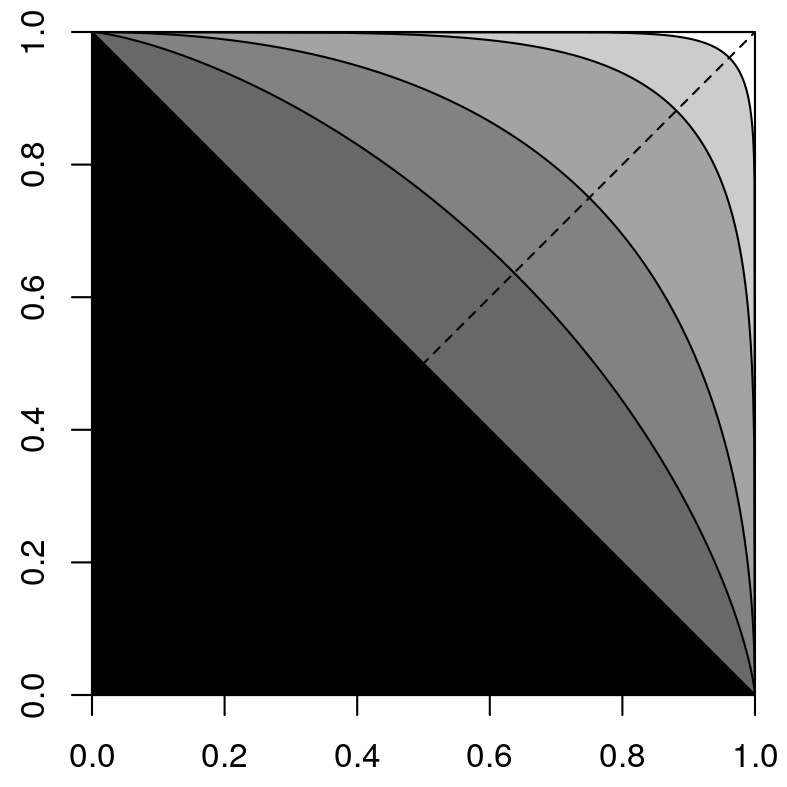
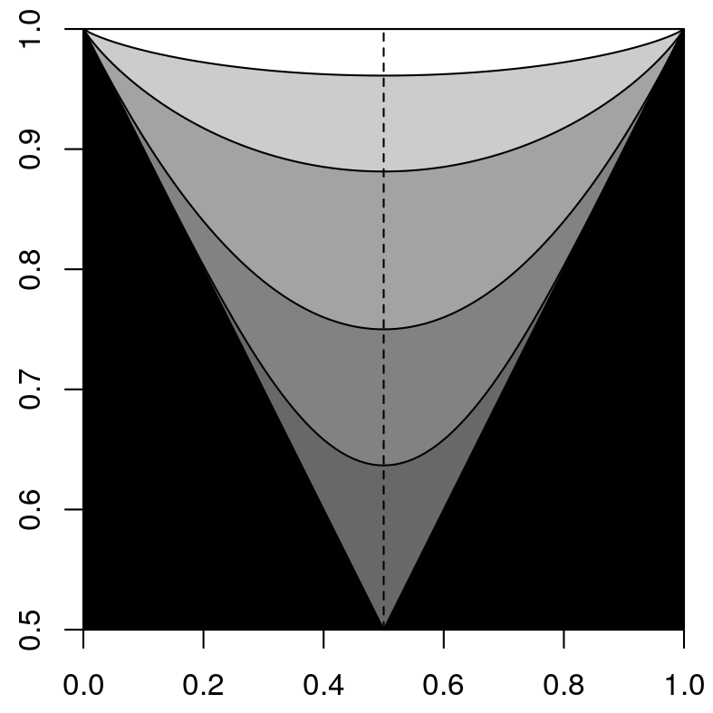
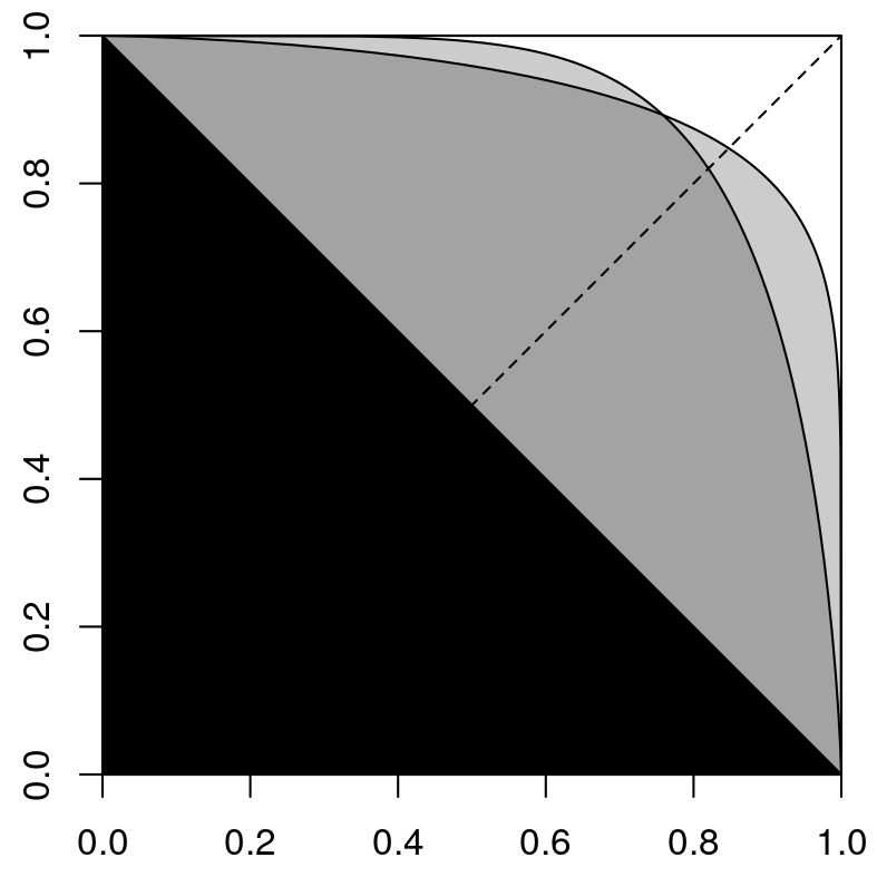
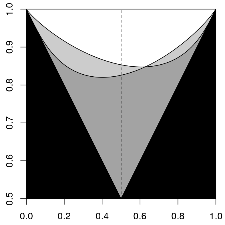
Figure 4: Top: Nested max-zonoids (left) and ordered (hypographs of) Pickands dependence functions (right) from the fully symmetric Dirichlet family for $\alpha\in\{0.0625,0.25,1,4\}$. Smaller values of $\alpha$ correspond to larger sets and larger Pickands dependence functions and are closer to the independence model represented by the box $[0,1]^{2}$ or the constant function, which is identically 1. The fully dependent model is represented in black. Bottom: Non-nested max-zonoids and non-ordered Pickands dependence function from the asymmetric Dirichlet family for $(\alpha_{1},\alpha_{2})\in\{(0.15,12),(4,0.2)\}$.

Here, we extend (15) in several ways: (i) going beyond the symmetric situation considering the fully asymmetric model, (ii) considering PQD/concordance order, (iii) shortening the proof by exploiting a connection to the theory of majorisation, cf. Appendix A.2. Figure 5 provides an illustration of the stochastic ordering for the asymmetric Dirichlet family in the bivariate case. In Figure 1 we see how the mass of the angular measure of the symmetric and asymmetric Dirichlet model is more concentrated from left plot to right plot. This also corresponds to their stochastic ordering, with the right one being the most dominant model in terms of PQD order.

Theorem 4.5 (PQD/concordance order of Dirichlet family).

Consider the max-stable Dirichlet family from Theorem/Definition 2.3. If ${\alpha}_{i}\leq{\beta}_{i}$, $i=1,\dots,d$, then

$$\mathrm{MaxDir}({\alpha_{1},\alpha_{2},\dots,\alpha_{d}})\leq_{\mathrm{PQD}}\mathrm{MaxDir}({\beta_{1},\beta_{2},\dots,\beta_{d}}).$$

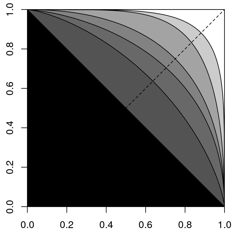
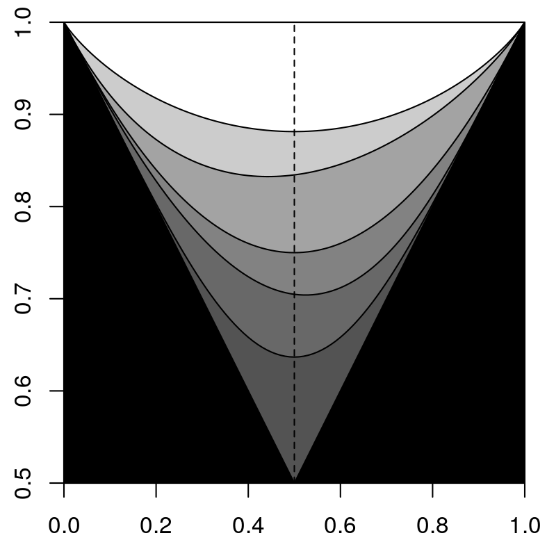
Figure 5: Nested max-zonoids and ordered Pickands dependence functions of the asymmetric max-stable Dirichlet family for $(\alpha_{1},\alpha_{2})\in\{(0.25,0.25),(1,0.25),(1,1),(1,4),(4,4)\}$. Componentwise smaller values of $(\alpha_{1},\alpha_{2})$ correspond to larger sets and larger Pickands dependence functions and are closer to the independence model.

Example 4.6.

In order to draw attention to some further consequences of Theorem 4.5, let ${\bm{X}}\sim\mathrm{MaxDir}({\bm{\alpha}})$ and ${\bm{Y}}\sim\mathrm{MaxDir}({\bm{\beta}})$ where $\alpha_{i}\leq\beta_{i}$, $i=1,\dots,d$, so that ${\bm{X}}\leq_{\mathrm{PQD}}{\bm{Y}}$, hence ${\bm{X}}\leq_{\mathrm{uo}}{\bm{Y}}$ and ${\bm{X}}\geq_{\mathrm{lo}}{\bm{Y}}$, which implies

$$\min_{i=1,\dots,d}(a_{i}X_{i})\leq_{\mathrm{st}}\min_{i=1,\dots,d}(a_{i}Y_{i})\qquad\text{for all ${\bm{a}}\in(0,\infty]^{d}$.}$$

$$\max_{i=1,\dots,d}(a_{i}X_{i})\leq_{\mathrm{st}}\max_{i=1,\dots,d}(a_{i}Y_{i})\qquad\text{for all ${\bm{a}}\in[0,\infty)^{d}$,}$$

cf. (12), (13) and Lemma 2.4. Exemplarily, we consider a range of trivariate symmetric and asymmetric max-stable Dirichlet distributions $\mathrm{MaxDir}(\alpha_{1},\alpha_{2},\alpha_{3})$ with parameters $(\alpha_{1},\alpha_{2},\alpha_{3})$ given in Figure 1. The colouring is chosen such that red models PQD-dominate blue models, which PQD-dominate black models.

In addition, we consider the portfolio with equal weights $(1,1,1)$ and the resulting min-projections $\min(X_{1},X_{2},X_{3})$ and max-projections $\max(X_{1},X_{2},X_{3})$, where $(X_{1},X_{2},X_{3})\sim\mathrm{MaxDir}(\alpha_{1},\alpha_{2},\alpha_{3})$. Figures 6 and 7 display their distribution functions on the Gumbel scale. As commonly of interest for extreme value distributions, instead of the quantile function $Q$, we show the equivalent return level plot, which displays the return levels $Q(1-p)$ for the return period of $1/p$ observations. The plots of these functions are based on empirical estimates from one million simulated observations from the respective models, and their orderings are as expected from the theory, i.e. quantile functions increase as the dominance of the model grows, while distribution functions decrease.

	Distribution functions	Return levels
Symmetric case
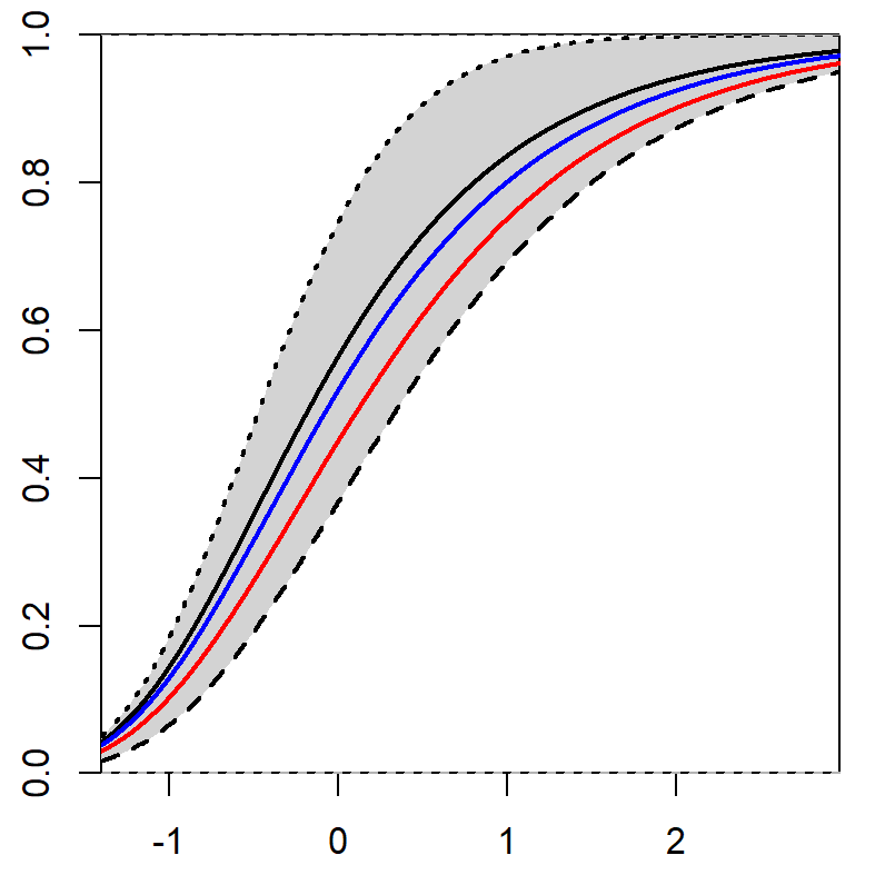
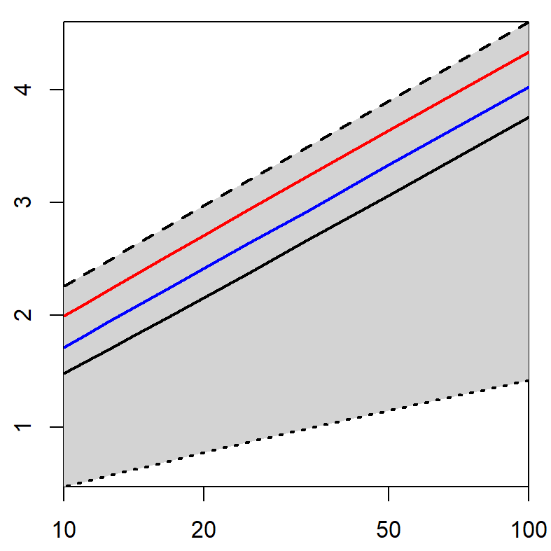
Asymmetric case

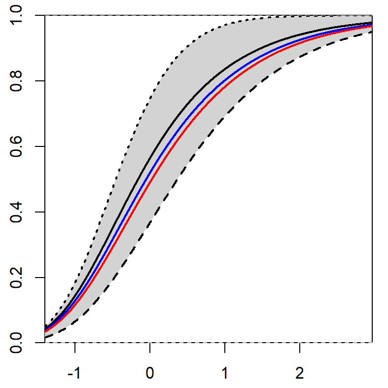
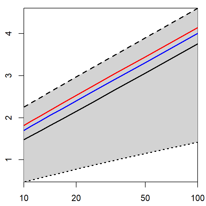
Figure 6: Distribution functions (left) and return levels (right) for return periods 10 to 100 (on logarithmic scale) of $\min(X_{1},X_{2},X_{3})$, where $(X_{1},X_{2},X_{3})\sim\mathrm{MaxDir}(\alpha_{1},\alpha_{2},\alpha_{3})$ on standard Gumbel scale with ${\bm{\alpha}}=(\alpha_{1},\alpha_{2},\alpha_{3})$ as chosen in Figure 1. Top: symmetric case; bottom: asymmetric case. Black, blue and red colouring encodes the matching with Figure 1. The grey areas represent the range between the fully dependent (dashed line) and fully independent (dotted line) cases.

	Distribution functions	Return levels
Symmetric case
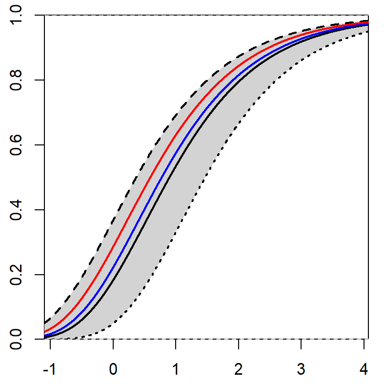
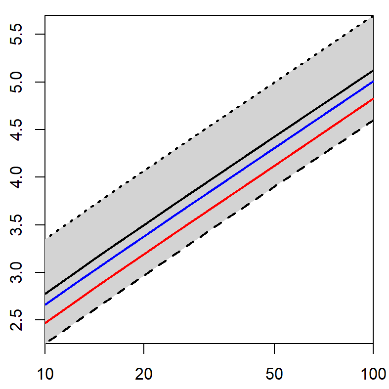
Asymmetric case

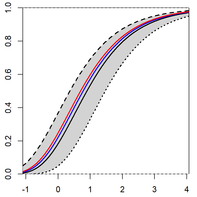
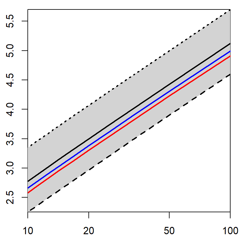
Figure 7: Distribution functions (left) and return levels (right) for return periods 10 to 100 (on logarithmic scale) of $\max(X_{1},X_{2},X_{3})$, where $(X_{1},X_{2},X_{3})\sim\mathrm{MaxDir}(\alpha_{1},\alpha_{2},\alpha_{3})$ on standard Gumbel scale with ${\bm{\alpha}}=(\alpha_{1},\alpha_{2},\alpha_{3})$ as chosen in Figure 1. Top: symmetric case; bottom: asymmetric case. Black, blue and red colouring encodes the matching with Figure 1. The grey areas represent the range between the fully dependent (dashed line) and fully independent (dotted line) cases.

Another prominent family of multivariate max-stable distributions that turns out to be stochastically ordered in the PQD/concordance order is the Hüsler-Reiß family. It can be shown using the limit result from Theorem 2.7 together with Slepian’s normal comparison lemma and some closure properties of the PQD/concordance order. Figure 8 provides an illustration in terms of nested max-zonoids and ordered Pickands dependence functions in the bivariate case. However, while these models are ordered, we would like to point out that none of the typically chosen families of log-Gaussian generators satisfy any of the orthant orders, cf. Example 4.11.

Theorem 4.7 (PQD/concordance order of Hüsler-Reiß family).

Consider the max-stable Hüsler-Reiß family from Theorem/Definition 2.5. If ${\gamma}_{i,j}\leq{\widetilde{\gamma}}_{i,j}$ for all $i,j\in\{1,\dots,d\}$, then

$$\mathrm{HR}({\bm{\gamma}})\geq_{\mathrm{PQD}}\mathrm{HR}(\widetilde{\bm{\gamma}}).$$

Remark 4.8.

With almost identical proof, cf. Appendix A.2, we may even deduce

$$\mathrm{HR}({\bm{\gamma}})\geq_{\mathrm{sm}}\mathrm{HR}(\widetilde{\bm{\gamma}}),$$

where $\geq_{\mathrm{sm}}$ denotes the supermodular order, cf. Müller and Stoyan (2002) Section 3.9 or Shaked and Shanthikumar (2007) Section 9.A.4. We have therefore included the respective arguments in the proof, too, although considering the supermodular order is otherwise beyond the scope of this article.

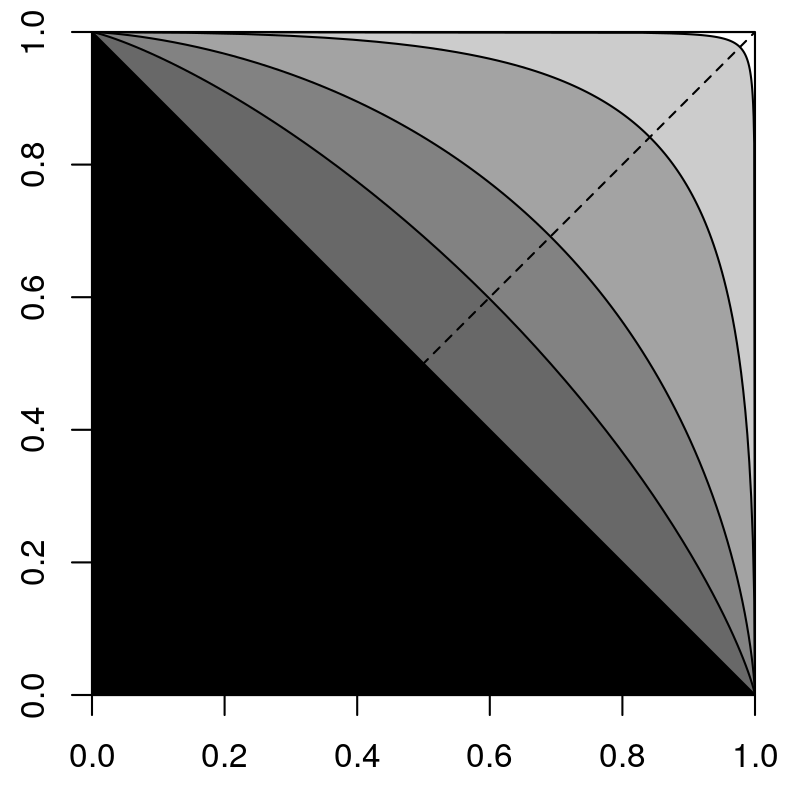
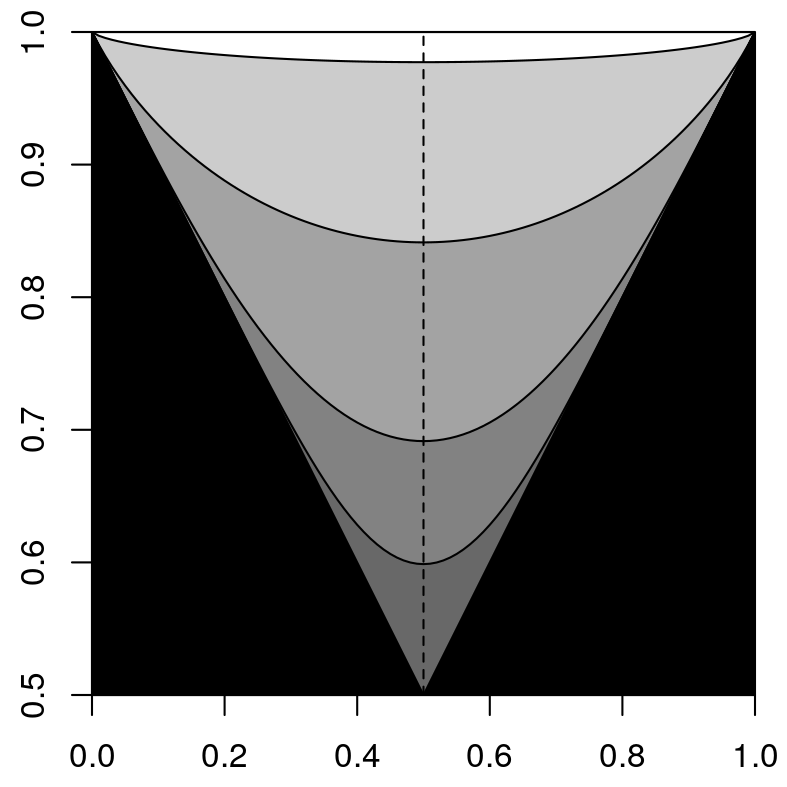
Figure 8: Nested max-zonoids and ordered Pickands dependence functions from the bivariate Hüsler-Reiß family for $\sqrt{\gamma}\in\{0.5,1,2,4\}$. Larger values of $\gamma$ correspond to larger sets and larger Pickands dependence functions and are closer to the independence model.

Remark 4.9.

Theorem 4.7 includes the assumption that both parameter matrices ${\bm{\gamma}}$ and $\widetilde{\bm{\gamma}}$ constitute a valid set of parameters for the Hüsler-Reiß model, i.e. they need to be elements of $\mathcal{G}_{d}$. In dimensions $d\geq 3$ it is possible that increasing (or decreasing) any of the parameters of a given valid ${\bm{\gamma}}$ will result in a set of parameters that is not valid for the Hüsler-Reiß model.

Remark 4.10.

Since the orthant orders are closed under independent conjunction, Theorem 4.7 extends to the generalised Hüsler-Reiß model, where we can allow some parameter values of ${\bm{\gamma}}$ to assume the value $\infty$, as long as ${\bm{\gamma}}$ remains negative definite in the extended sense (see Remark 2.8).

Example 4.11 (Ordering of $G$/$\widetilde{G}$ does not imply generator ordering for ${\bm{Z}}$/$\widetilde{\bm{Z}}$ – the case of Hüsler-Reiß log-Gaussian generators).

Consider the non-degenarate bivariate Hüsler-Reiß model with $\gamma_{12}=\gamma_{21}=\gamma\in(0,\infty)$ and let additionally $a\in[0,1]$. Then the zero mean bivariate Gaussian model $(W_{1},W_{2})^{\top}$ with $\mathbb{E}(W_{1})=\gamma a^{2}$, $\mathbb{E}(W_{2})=\gamma(1-a)^{2}$, $\mathrm{Cov}(W_{1},W_{2})=0.5\gamma\cdot(a^{2}+(1-a)^{2}-1)$ satisfies $\mathbb{E}(W_{1}-W_{2})^{2}=\gamma$, hence leads to a generator for the bivariate Hüsler-Reiß distribution in the sense of Theorem/Definition 2.5. WLOG $a\in(0,1]$ (otherwise consider $1-a$ instead of $a$). Then $\log(Z_{1})$ follows a non-degenerate univariate Gaussian distribution with mean $-0.5\gamma a^{2}$ and variance $\gamma a^{2}$. The family of such distributions is not ordered in $\gamma>0$ (cf. e.g. Shaked and Shanthikumar (2007) Example 1.A.26 or Müller and Stoyan (2002) Theorem 3.3.13). Hence, the bivariate family $(\log(Z_{1}),\log(Z_{2}))^{\top}$ can also not be ordered according to orthant order, nor can any multivariate family, for which this constitutes a marginal family. Accordingly, the corresponding log-Gaussian generators ${\bm{Z}}$ of the Hüsler-Reiß model will not be ordered, even when the resulting max-stable model and exponent measures are ordered as seen in Theorem 4.7.

While Dirichlet and Hüsler-Reiß families are ordered in the PQD/concordance sense according to the natural ordering of their parameter spaces, we would like to provide some examples that show that UO and LO ordering among simple max-stable distributions are in fact not equivalent.

To this end, we revisit the Choquet max-stable model from Section 2.2.3. We write $\mathrm{Choquet}_{\mathrm{EC}}(\theta)$ for the simple max-stable Choquet distribution if it is parameterised by its extremal coefficients $\theta(A)$, $A\subset\{1,\dots,d\}$, $A\neq\emptyset$ and $\mathrm{Choquet}_{\mathrm{TD}}(\chi)$ if it is parameterised by its tail dependence coefficients $\chi(A)$, $A\subset\{1,\dots,d\}$, $A\neq\emptyset$.

Lemma 4.12 (LO and UO order of Choquet family/Tawn-Molchanov model).

Consider the family of max-stable Choquet models from Section 2.2.3. Then the LO order is characterised by the ordering of extremal coefficients, we have

$$\theta\leq\widetilde{\theta}\qquad \iff\qquad\mathrm{Choquet}_{\mathrm{EC}}(\theta)\leq_{\mathrm{lo}}\mathrm{Choquet}_{\mathrm{EC}}(\widetilde{\theta});$$

and the UO order is characterised by the ordering of tail dependence coefficients, that is

$$\chi\leq\widetilde{\chi}\qquad \iff\qquad\mathrm{Choquet}_{\mathrm{TD}}(\chi)\leq_{\mathrm{uo}}\mathrm{Choquet}_{\mathrm{TD}}(\widetilde{\chi}).$$

As we know already from Theorem 4.1 part c), in dimension $d=2$, it is easily seen that $\chi\leq\widetilde{\chi}$ is equivalent to $\theta\geq\widetilde{\theta}$, alternatively recall $\theta_{12}+\chi_{12}=2$. Starting from dimension $d=3$, this is no longer the case and one can easily construct examples, where only LO or UO ordering holds.

Example 4.13.

Table 1 lists valid parameter sets for four different trivariate Choquet models. Among these, we can easily read off that

• $B\leq_{\mathrm{uo}}D$, but there is no order between $B$ and $D$ according to lower orthants;

• $C\leq_{\mathrm{lo}}B$, but there is no order between $B$ and $C$ according to upper orthants.

Of course, it is still possible that Choquet models are ordered according to PQD order, e.g.

• $A\leq_{\mathrm{PQD}}B$.

It is also possible to have both LO and UO order in the same direction, e.g.

• $A\leq_{\mathrm{uo}}C$ and $A\leq_{\mathrm{lo}}C$.

However, note that such an order can only arise if the bivariate marginal distributions all agree.

	$\tau_{1}$	$\tau_{12}$	$\tau_{123}$	$\chi_{12}$	$\chi_{123}$	$\theta_{12}$	$\theta_{123}$
A	0.3	0.2	0.3	0.5	0.3	1.5	1.8
B	0.1	0.3	0.3	0.6	0.3	1.4	1.5
C	0.4	0.1	0.4	0.5	0.4	1.5	1.9
D	0.3	0.0	0.7	0.7	0.7	1.3	1.6

Table 1: Valid parameter sets of trivariate Choquet models, cf. Section 2.2.3, that are exchangeable so that parameters $\tau_{A}$, $\chi_{A}$, $\theta_{A}$ depend on sets $A$ only through their cardinality. Since $\chi_{1}=\theta_{1}=1$ these parameters need not be listed. We have $\tau_{1}+2\tau_{12}+\tau_{123}=1$, $\chi_{123}=\tau_{123}$, $\chi_{12}=\chi_{123}+\tau_{12}$, $\theta_{12}=1+\tau_{1}+\tau_{12}$ and $\theta_{123}=\theta_{12}+\tau_{1}$.

Acknowledgements

We would like to thank two anonymous referees who have positively challenged us in two directions: (i) not only considering the order according to lower orthants, but to study the PQD-order, and (ii) extending the bivariate to the multivariate Hüsler-Reiß model. Their encouragement to pursue these routes has helped us to significantly broaden the scope of this work. MC thankfully acknowledges funding from the Maths DTP 2020 – Engineering and Physical Sciences Research Council grant EP/V520159/1 – at the School of Mathematics of Cardiff University.

Appendix A Proofs

A.1 Proofs concerning fundamental order relations

Proof of Theorem 4.1.

In what follows, let ${\bm{X}}\sim G$ and $\widetilde{\bm{X}}\sim\widetilde{G}$.

a) Because of (13), it suffices to compare $G({\bm{x}})$ and $\widetilde{G}({\bm{x}})$ for ${\bm{x}}\in(0,\infty)^{d}$ only. The same is true for $\ell$ and $\widetilde{\ell}$ as they are continuous on $[0,\infty)^{d}$. At the same time the test sets for the relation $\Lambda\leq_{\mathrm{lo}}\widetilde{\Lambda}$ in Definition 3.2 are precisely of the form $\mathbb{R}^{d}\setminus L_{{\bm{x}}}$, where ${\bm{x}}\in(0,\infty)^{d}$. So the equivalence of (i), (ii), (iii) and (iv) follows directly from the relations

$$G({\bm{x}})=\mathbb{P}({\bm{X}}\in L_{\bm{x}})=\exp(-\Lambda([0,\infty]^{d}\setminus L_{\bm{x}}))=\exp(-\Lambda(\mathbb{R}^{d}\setminus L_{\bm{x}}))$$

with

$$\Lambda(\mathbb{R}^{d}\setminus L_{\bm{x}})=\ell(1/x_{1},\dots,1/x_{d})=\mathbb{E}(\max(Z_{1}/x_{1},\dots,Z_{d}/x_{d})),$$

and the respective tilde-counterparts. Likewise, the equivalence of (iv) and (v) is immediate from (3) and (2).

b) We start by showing the equivalence between (ii) and (iii). The test sets for the relation $\Lambda\leq_{\mathrm{uo}}\widetilde{\Lambda}$ in Definition 3.2 are precisely the upper orthants $U_{{\bm{x}}}$, where at least one component of ${\bm{x}}$ is larger than zero. Let ${\bm{a}}\in(0,\infty)^{d}$ and $A\subset\{1,\dots,d\}$, $A\neq\emptyset$. Define ${\bm{x}}\in\mathbb{R}^{d}$ by setting $x_{i}=1/a_{i}$ if $i\in A$ and $x_{i}=-1$ else. Then $U_{\bm{x}}$ is an admissible test set and

$$\Lambda(U_{\bm{x}})=\Lambda\bigg{(}\Big{\{}{\bm{y}}\in[0,\infty)^{d}\setminus\{{\bm{0}}\}\,:\,\min_{i\in A}(a_{i}y_{i})>1\Big{\}}\bigg{)}=\mathbb{E}\Big{(}\min_{i\in A}(a_{i}Z_{i})\Big{)}.$$ (16)

Likewise, $\widetilde{\Lambda}(U_{\bm{x}})=\mathbb{E}(\min_{i\in A}(a_{i}\widetilde{Z}_{i}))$ and we may deduce the implication (ii)$\Rightarrow$(iii). Conversely, assume (iii) and note that the same argument implies $\Lambda(U_{\bm{x}})\leq\widetilde{\Lambda}(U_{\bm{x}})$ for any ${\bm{x}}$, which has at least one positive component, whilst all other components of ${\bm{x}}$ are negative. What remains to be seen is the same relation for upper orthants $U_{\bm{x}}$, for which at least one component of ${\bm{x}}$ is positive, but where among the non-positive components, there may be zeroes. Let ${\bm{x}}\in\mathbb{R}^{d}$ be such a vector. For $n\in\mathbb{N}$ let ${\bm{x}}_{n}\in\mathbb{R}^{d}$ be an identical vector, but with zero entries replaced by $1/n$. Then $\Lambda(U_{{\bm{x}}_{n}})\leq\widetilde{\Lambda}(U_{{\bm{x}}_{n}})$ for all $n\in\mathbb{N}$ by the previous argument, whilst $U_{{\bm{x}}_{n}}\uparrow U_{\bm{x}}$, such that $\Lambda(U_{{\bm{x}}_{n}})\to\Lambda(U_{{\bm{x}}})$ and $\widetilde{\Lambda}(U_{{\bm{x}}_{n}})\to\widetilde{\Lambda}(U_{{\bm{x}}})$ as $n\to\infty$. This shows (iii)$\Rightarrow$(ii).

Next, we establish (i)$\Rightarrow$(iii). Assume (i). Since the order UO is closed under marginalisation, it suffices to consider $A=\{1,\dots,d\}$ in (iii), see also Lemma 2.2. Set $x_{i}=1/a_{i}$, $i=1,\dots,d$, such that (16) holds (as well as the tilde-version) and note that the closure of $U_{\bm{x}}$ in $[0,\infty]^{d}\setminus\{{\bm{0}}\}$ is a continuity set for each of the $(-1)$-homogeneous measures $\Lambda$ and $\widetilde{\Lambda}$. Hence, since each max-stable vector satisfies its own Domain-of-attraction conditions (cf. e.g. Resnick (1987) Section 5.4.2), we have

$$\Lambda(U_{\bm{x}})=\lim_{n\to\infty}n\mathbb{P}({\bm{X}}\in nU_{\bm{x}})=\lim_{n\to\infty}n\mathbb{P}({\bm{X}}\in U_{n{\bm{x}}})$$

and the analog for $\widetilde{\Lambda}$ and $\widetilde{\bm{X}}$. The implication (i)$\Rightarrow$(iii) follows.

Lastly, let us establish (iii)$\Rightarrow$(i). Suppose (iii) holds. We abbreviate $\chi^{(a)}(A)=\mathbb{E}(\min_{i\in A}(a_{i}Z_{i}))$ and analogously $\widetilde{\chi}^{(a)}(A)=\mathbb{E}(\min_{i\in A}(a_{i}\widetilde{Z}_{i}))$, such that (iii) translates into

$$\chi^{(a)}(A)\leq\widetilde{\chi}^{(a)}(A)$$

for all ${\bm{a}}\in(0,\infty)^{d}$ and $A\subset\{1,\dots,d\}$, $A\neq\emptyset$. With $\theta^{(a)}(A)=\mathbb{E}(\max_{i\in A}(a_{i}Z_{i}))$ we find that

$$\chi^{(a)}(A)=\sum_{I\subset A,\,I\neq\emptyset}(-1)^{|I|+1}\theta^{(a)}(I)\qquad\text{and}\qquad\theta^{(a)}(A)=\sum_{I\subset A,\,I\neq\emptyset}(-1)^{|I|+1}\chi^{(a)}(I)$$

(similarly to (9) and analogously for the tilde-version), where $\theta^{(a)}$ can be interpreted as directional extremal coefficient function. It is easily seen that $\theta^{(a)}$ with $\theta^{(a)}(\emptyset)=0$ is union-completely alternating, cf. Lemma B.3.

Because of (12), in order to arrive at (i), it suffices to establish

$$\mathbb{P}\Big{(}\min_{i=1,\dots,d}(a_{i}X_{i})>1\Big{)}\leq\mathbb{P}\Big{(}\min_{i=1,\dots,d}(a_{i}\widetilde{X}_{i})>1\Big{)}$$

for all ${\bm{a}}\in(0,\infty)^{d}$. In the notation of Lemma B.3 and with $g(x)=1-\exp(-x)$, the left-hand side can be rewritten as

$$\mathbb{P}\Big{(}\min_{i=1,\dots,d}(a_{i}X_{i})>1\Big{)} =1-\sum_{I\subset\{1,\dots,d\},\,I\neq\emptyset}(-1)^{|I|+1}\mathbb{P}\Big{(}\max_{i\in I}(a_{i}X_{i})\leq 1\Big{)}$$

$$=-\sum_{I\subset\{1,\dots,d\}}(-1)^{|I|+1}\exp\big{(}-\ell({\bm{a}}_{I})\big{)}$$

$$=\sum_{I\subset\{1,\dots,d\}}(-1)^{|I|+1}-\sum_{I\subset\{1,\dots,d\}}(-1)^{|I|+1}\exp\big{(}-\theta^{(a)}(I)\big{)}$$

$$=\sum_{I\subset\{1,\dots,d\}}(-1)^{|I|+1}g\big{(}\theta^{(a)}(I)\big{)}$$

(and analogously for the tilde-version). The assertion follows then directly from Proposition B.9, since $g$ is a Bernstein function.

c) The statement follows from the relation

$$\mathbb{E}(\min(a_{1}Z_{1},a_{2}Z_{2}))+\mathbb{E}(\max(a_{1}Z_{1},a_{2}Z_{2}))=\mathbb{E}(\min(a_{1}\widetilde{Z}_{1},a_{2}\widetilde{Z}_{2}))+\mathbb{E}(\max(a_{1}\widetilde{Z}_{1},a_{2}\widetilde{Z}_{2})),$$

as both sides are equal to $a_{1}+a_{2}$. ∎

Proof of Corollary 4.3.

In view of (14) and Theorem 4.1 b), if suffices to investigate the upper and lower bounds of $\mathbb{E}(\min_{i\in A}(a_{i}Z_{i}))$ for ${\bm{a}}\in(0,\infty)^{d}$ and $A\subset\{1,\dots,d\}$, $A\neq\emptyset$, where ${\bm{Z}}$ is a generator for $G$. We have

$$\mathbb{E}\big{(}\min_{i\in A}(a_{i}Z_{i})\big{)} \leq\min_{i\in A}(\mathbb{E}(a_{i}Z_{i}))=\min_{i\in A}(a_{i})\qquad\text{and}\qquad\mathbb{E}\big{(}\min_{i\in A}(a_{i}Z_{i})\big{)}\geq\begin{cases}a_{j}&\text{if }A=\{j\},\\ 0&\text{else},\end{cases}$$

and the upper and lower bounds are attained by generators of the fully dependent model (${\bm{Z}}$ being almost surely ${\bm{e}}=(1,1,\dots,1)^{\top}$) and the independent model (${\bm{Z}}$ being uniformly distributed among the set $\{d{\bm{e}_{1}},d{\bm{e}_{2}},\dots,d{\bm{e}}_{d}\}$), respectively, which implies the assertion. ∎

Proof of Corollary 4.4.

The lower orthant order ${\bm{X}}^{*}\,\geq_{\mathrm{lo}}\,{\bm{X}}$ is known from Theorem 2.9. Let ${\bm{Z}}$ and ${\bm{Z}}^{*}$ be generators of the respective models. Since they share identical extremal coefficients, they also share identical tail dependence coefficients $\chi(A)=\mathbb{E}(\min_{i\in A}Z_{i})=\mathbb{E}(\min_{i\in A}Z^{*}_{i})$, $A\subset\{1,\dots,d\}$, $A\neq\emptyset$, which can be retrieved from $\theta$ via (9). In general, we have for $A\subset\{1,\dots,d\}$, $A\neq\emptyset$, ${\bm{a}}\in(0,\infty)^{d}$

$$\mathbb{E}\big{(}\min_{i\in A}(a_{i}Z_{i})\big{)}\geq\min_{i\in A}(a_{i})\mathbb{E}\big{(}\min_{i\in A}(Z_{i})\big{)}=\min_{i\in A}(a_{i})\cdot\chi(A).$$

The Choquet model attains the lower bound, since with (7) and (11)

$$\mathbb{E}\big{(}\min_{i\in A}(a_{i}Z^{*}_{i})\big{)} =\sum_{L\subset\{1,\dots,d\},L\neq\{\emptyset\}}\tau(L)\min_{i\in A}(a_{i}({\bm{e}}_{L})_{i})$$

$$=\sum_{L\subset\{1,\dots,d\},A\subset L}\tau(L)\min_{i\in A}(a_{i})=\min_{i\in A}(a_{i})\cdot\chi(A).$$

So by Theorem 4.1 we also have ${\bm{X}}^{*}\,\leq_{\mathrm{uo}}\,{\bm{X}}$, hence the assertion. ∎

Proof of Lemma 4.12.

The LO part is immediate from $\theta\leq\widetilde{\theta}$ implying the inclusion of associated max-zonoids $K^{*}\subset\widetilde{K}^{*}$ or Choquet integrals $\ell^{*}\leq\widetilde{\ell}^{*}$ (cf. Theorem 2.9) and then follows directly from Theorem 4.1 part a). For the UO part, note from the Proof of Corollary 4.4 that for $A\subset\{1,\dots,d\}$, $A\neq\emptyset$, ${\bm{a}}\in(0,\infty)^{d}$

$$\mathbb{E}\big{(}\min_{i\in A}(a_{i}Z^{*}_{i})\big{)}=\min_{i\in A}(a_{i})\cdot\chi(A)\qquad\text{and}\qquad\mathbb{E}\big{(}\min_{i\in A}(a_{i}\widetilde{Z}^{*}_{i})\big{)}=\min_{i\in A}(a_{i})\cdot\widetilde{\chi}(A)$$

if ${\bm{Z}}$ and $\widetilde{\bm{Z}}$ are generators of the respective models, hence the assertion with Theorem 4.1 part b). ∎

A.2 Proofs concerning the Dirichlet and Hüsler-Reiß models

Proof of Theorem 2.3.

The equivalence of (ii) and (iii) has been verified in Coles and Tawn (1991). The equivalence of (i) and (ii) follows similarly to Aulbach et al. (2015) (3) from the fact that ${\bm{D}}$ is distributed like ${\bm{\Gamma}}/\lVert{\bm{\Gamma}}\lVert_{1}$ and the independence of ${\bm{\Gamma}}/\lVert{\bm{\Gamma}}\rVert_{1}$ and $\lVert{\bm{\Gamma}}\rVert_{1}$. More precisely, let $\ell_{1}$ and $\ell_{2}$ be the stable tail dependence functions that arise from the generators (i) and (ii), respectively. Then $\ell_{1}$ and $\ell_{2}$ can be expressed as follows for any ${\bm{x}}\in[0,\infty)^{d}$

$$\ell_{1}({\bm{x}}) =\mathbb{E}\max_{i=1,\dots,d}\frac{x_{i}\Gamma_{i}}{\alpha_{i}}={\mathbb{E}\lVert{\bm{\Gamma}}\rVert_{1}}\cdot\mathbb{E}\max_{i=1,\dots,d}\frac{x_{i}\Gamma_{i}/\lVert{\bm{\Gamma}}\rVert_{1}}{\alpha_{i}},$$

$$\ell_{2}({\bm{x}}) =\mathbb{E}\max_{i=1,\dots,d}\frac{x_{i}\lVert{\bm{\alpha}}\rVert_{1}D_{i}}{\alpha_{i}}=\lVert{\bm{\alpha}}\rVert_{1}\cdot\mathbb{E}\max_{i=1,\dots,d}\frac{x_{i}D_{i}}{\alpha_{i}}.$$

If suffices to note $\mathbb{E}\lVert{\bm{\Gamma}}\rVert_{1}=\lVert{\bm{\alpha}}\rVert_{1}$ in order to conclude $\ell_{1}=\ell_{2}$. ∎

In order to prove Theorem 4.5 we will use a simple inequality that follows from the theory of majorisation (Marshall et al., 2011).

Proposition A.1 (Marshall and Proschan (1965) Corollary 3, Marshall et al. (2011) Proposition B.2.b.).

Let $g:\mathbb{R}\to\mathbb{R}$ be continuous and convex and let $X_{1},X_{2},\dots$ be a sequence of independent and identically distributed random variables, then

$$\mathbb{E}\,g\bigg{(}\sum_{i=1}^{n}\frac{X_{i}}{n}\bigg{)}$$

is nonincreasing in $n=1,2,\dots$.

Corollary A.2.

Let $g:\mathbb{R}\to\mathbb{R}$ be continuous and convex and, let $Z^{(\alpha)}\sim\Gamma(\alpha)$ follow a univariate Gamma distribution with shape parameter $\alpha>0$, then

$$\mathbb{E}\,g\bigg{(}\frac{Z^{(\alpha)}}{\alpha}\bigg{)}$$

is nonincreasing in $\alpha\in(0,\infty)$.

Proof.

We consider first the case that $\alpha=(k/n)\cdot\beta$ for some natural numbers $1\leq k<n$. Then consider independent and identically distributed random variables $\Gamma_{1},\Gamma_{2},\dots$ following a $\Gamma(\beta/n)$ distribution. Then Proposition A.1 gives

$$\mathbb{E}\,g\bigg{(}\frac{\sum_{i=1}^{k}\Gamma_{i}}{\alpha}\bigg{)}=\mathbb{E}\,g\bigg{(}\frac{n}{\beta}\cdot\sum_{i=1}^{k}\frac{\Gamma_{i}}{k}\bigg{)}\geq\mathbb{E}\,g\bigg{(}\frac{n}{\beta}\cdot\sum_{i=1}^{n}\frac{\Gamma_{i}}{n}\bigg{)}=\mathbb{E}\,g\bigg{(}\frac{\sum_{i=1}^{n}\Gamma_{i}}{\beta}\bigg{)}.$$

By the convolution stability of the Gamma distribution

$$\sum_{i=1}^{k}\Gamma_{i}\sim\Gamma(\alpha)\qquad\text{and}\qquad\sum_{i=1}^{n}\Gamma_{i}\sim\Gamma(\beta).$$

Hence, the assertion is shown for $\alpha$ and $\beta$ that differ by a rational multiplier.

If we only know $\alpha<\beta$, consider a decreasing sequence $\beta_{n}\downarrow\beta$, such that $\alpha$ and $\beta_{n}$ differ by a rational multiplier. This gives $\mathbb{E}g({Z^{(\alpha)}}/{\alpha})\geq\limsup_{n\to\infty}\mathbb{E}g({Z^{(\beta_{n})}}/{\beta_{n}})$ by the above argument. On the other hand, Fatou’s lemma gives $\mathbb{E}g({Z^{(\beta)}}/{\beta})\leq\liminf_{n\to\infty}\mathbb{E}g({Z^{(\beta_{n})}}/{\beta_{n}})$. This finishes the proof. ∎

Proof of Theorem 4.5.

If ${\bm{\alpha}}={\bm{\beta}}$, the statement is clear. Else, because the parameter space of the Dirichlet model is $(0,\infty)^{d}$, we can find a chain of parameter vectors ${\bm{\alpha}}={\bm{\alpha}}^{(0)}\leq{\bm{\alpha}}^{(1)}\leq\dots\leq{\bm{\alpha}}^{(m)}={\bm{\beta}}$, such that for each $i=0,\dots,m-1$, the vectors ${\bm{\alpha}}^{(i)}$ and ${\bm{\alpha}}^{(i+1)}$ differ only by one component. Hence it suffices to consider the case, where ${\bm{\alpha}}$ and ${\bm{\beta}}$ differ only in one component. Without loss of generality, let this be the first component.

Let ${\bm{Z}}$ be a Gamma generator for $\mathrm{MaxDir}({\bm{\alpha}})$ and $\widetilde{\bm{Z}}$ be a Gamma generator for for $\mathrm{MaxDir}({\bm{\beta}})$ in the sense of Theorem/Definition 2.3. Then we may assume that $Z_{i}=\widetilde{Z}_{i}$ for $i=2,\dots,d$, whereas $\alpha_{1}Z_{1}\sim\Gamma(\alpha_{1})$ and $\beta_{1}\widetilde{Z}_{1}\sim\Gamma(\beta_{1})$ are independent from $(Z_{2},\dots,Z_{d})^{\top}$, and $\alpha_{1}<\beta_{1}$ by assumption. We will need to show (cf. Theorem 4.1) that for fixed ${\bm{a}}\in(0,\infty)^{d}$ and $A\subset\{1,\dots,d\}$, $A\neq\emptyset$

$$\mathbb{E}\min_{i\in A}\big{(}a_{i}Z_{i}\big{)}\leq\mathbb{E}\min_{i\in A}\big{(}a_{i}\widetilde{Z}_{i}\big{)}\qquad\text{and}\qquad\mathbb{E}\max_{i=1,\dots,d}\big{(}a_{i}Z_{i}\big{)}\geq\mathbb{E}\max_{i=1,\dots,d}\big{(}a_{i}\widetilde{Z}_{i}\big{)}.$$

Due to the setting above, it suffices to consider only subsets $A$ with $1\in A$, and due to the marginal standardisation $\mathbb{E}(Z_{1})=1$, it suffices to restrict our attention to $A\setminus\{1\}\neq\emptyset$. Setting $V_{A}=\min_{i\in A\setminus\{1\}}{(a_{i}Z_{i})}$ and $W=\max_{i=2,\dots,d}{(a_{i}Z_{i})}$ this means the assertion will follow from

$$\mathbb{E}\min\big{(}a_{1}Z_{1},V_{A}\big{)}\leq\mathbb{E}\min\big{(}a_{1}\widetilde{Z}_{1},V_{A}\big{)}\qquad\text{and}\qquad\mathbb{E}\max\big{(}a_{1}Z_{1},W\big{)}\geq\mathbb{E}\max\big{(}a_{1}\widetilde{Z}_{1},W\big{)}.$$

Indeed, this is implied by Corollary A.2, when considering the continuous convex functions $g_{c}(x)=-\min(a_{1}x,c)$ or $g_{c}(x)=\max(a_{1}x,c)$ for a constant $c\in\mathbb{R}$. ∎

Proof of Theorem 4.7.

Set

$$\rho_{ij}^{(n)}=\exp(-\gamma_{ij}/(4\log(n))\qquad\text{and}\qquad\widetilde{\rho}_{ij}^{(n)}=\exp(-\widetilde{\gamma}_{ij}/(4\log(n))$$

for $i,j\in\{1,\dots,d\}$, $n\in\mathbb{N}$, so that ${\bm{\gamma}},{\widetilde{\bm{\gamma}}}\in\mathcal{G}_{d}$ ensures that the resulting matrices are correlation matrices, cf. e.g. Berg et al. (1984) Theorem 3.2.2. By construction, $\rho_{ij}^{(n)}\geq\widetilde{\rho}_{ij}^{(n)}$ for all $i,j,n$. And so the normal comparison lemma (Slepian, 1962), cf. also Tong (1980) Section 2.1. or Müller and Stoyan (2002) Example 3.8.6, implies that ${\bm{Y}}\geq_{\mathrm{PQD}}\widetilde{\bm{Y}}$ if ${\bm{Y}}$ and $\widetilde{\bm{Y}}$ are zero mean unit-variance Gaussian random vectors with correlations ${\bm{\rho}}$ and $\widetilde{\bm{\rho}}$, respectively. In fact, even ${\bm{Y}}\geq_{\mathrm{sm}}\widetilde{\bm{Y}}$ holds for the supermodular order (Müller and Stoyan, 2002, Theorem 3.13.5).

Consider the triangular arrays with independent ${\bm{Y}}^{(n)}_{i}\sim{\bm{Y}}$, $i=1,\dots,n$ and $\widetilde{\bm{Y}}^{(n)}_{i}\sim\widetilde{\bm{Y}}$, $i=1,\dots,n$. Since $t(1-\exp(-a/t))\to a$ as $t\to\infty$, Theorem 2.7 gives that

$$u_{n}({\bm{M}}^{(n)}-u_{n})=u_{n}\cdot\bigg{(}\max_{i=1,\dots,n}({\bm{Y}}^{(n)}_{i})_{1}-u_{n},\dots,\max_{i=1,\dots,n}({\bm{Y}}^{(n)}_{i})_{d}-u_{n}\bigg{)}^{\top}$$

converges in distribution to $\mathrm{HR}({\bm{\gamma}})$ and the corresponding tilde-version, while the closure under independent conjunction (Shaked and Shanthikumar (2007) Theorem 9.A.5) together with Shaked and Shanthikumar (2007) Theorem 9.A.4 implies $u_{n}({\bm{M}}^{(n)}-u_{n})\geq_{\mathrm{PQD}}u_{n}(\widetilde{\bm{M}}^{(n)}-u_{n})$ for all $n\in\mathbb{N}$. In fact, even $u_{n}({\bm{M}}^{(n)}-u_{n})\geq_{\mathrm{sm}}u_{n}(\widetilde{\bm{M}}^{(n)}-u_{n})$ for all $n\in\mathbb{N}$ as the supermodular order is also closed under independent conjuction (Müller and Stoyan, 2002, Theorem 3.9.14) and note Shaked and Shanthikumar (2007) Theorem 9.A.12. The assertion follows now from the closure of the PQD-order under distributional limits (Shaked and Shanthikumar (2007) Theorem 9.A.5). We even have $\mathrm{HR}({\bm{\gamma}})\geq_{\mathrm{sm}}\mathrm{HR}(\widetilde{\bm{\gamma}})$, as the supermodular order satisfies the same closure property with respect to distributional limits (Müller and Stoyan, 2002, Theorem 3.9.12). ∎

Appendix B Complete alternation and Bernstein functions

We recall some elementary definitions and facts from Berg et al. (1984), cf. also Molchanov (2017). Let $(S,\circ,e)$ be an abelian semigroup, that is, a non-empty set $S$ with a composition $\circ$ that is associative and commutative and has a neutral element $e$. Three examples are of interest to us:

1. $S=[0,\infty)$ with $+$ and neutral element $0$,

2. $S=\mathcal{P}_{d}$, the power set of $\{1,\dots,d\}$, with the union operation $\cup$ and neutral element $\emptyset$,

3. $S=[0,\infty)^{d}$ with the componentwise maximum operation $\vee$ and neutral element ${\bm{0}}$.

Examples (ii) and (iii) are even idempotent semigroups, as $s\circ s=s$ for these operations. We use the standard notation

$$(\Delta_{b}f)(a)=f(a)-f(a\circ b).$$

Definition B.1.

A function $f:S\to\mathbb{R}$ is called completely alternating if for all $n\geq 1$, $\{s_{1},\dots,s_{n}\}\subset S$ and $s\in S$

$$(\Delta_{s_{1}}\Delta_{s_{2}}\dots\Delta_{s_{n}}f)(s)=\sum_{I\subset\{1,\dots,n\}}(-1)^{|I|}f(s\circ\bigcirc_{i\in I}\,s_{i})\leq 0.$$

For idempotent semigroups (examples (ii) and (iii) above), the complete alternation property coincides with negative definiteness, cf. Berg et al. (1984) 4.4.16 and 4.6.8.

Definition B.2.

A function $f:S\to\mathbb{R}$ is called negative definite if for all $n\geq 2$, $\{s_{1},\dots,s_{n}\}\subset S$, $\{a_{1},\dots,a_{n}\}\subset\mathbb{R}$ with $a_{1}+\dots+a_{n}=0$

$$\sum_{j=1}^{n}\sum_{k=1}^{n}a_{j}a_{k}f(s_{j}\circ s_{k})\leq 0.$$

In the context of multivariate extremes, max-complete alternation of the stable tail dependence function implies union-complete alternation of the extremal coefficient function. In fact, the following directional version holds true irrespective of whether we take homogeneity or marginal standardisation into account or not.

Lemma B.3.

Let $\ell:[0,\infty)^{d}\to[0,\infty)$ be max-completely alternating. Let ${\bm{x}}\in[0,\infty)^{d}$. Let $\theta^{(x)}:\mathcal{P}_{d}\to[0,\infty)$ be defined as $\theta^{(x)}(A)=\ell({\bm{x}}_{A})$, where ${\bm{x}}_{A}={\bm{x}}\cdot{\bm{e}}_{A}\in[0,\infty)^{d}$ is the vector with $x_{i}$ as $i$-th coordinate if $i\in A$ and zero else. Then $\theta^{(x)}$ is union-completely alternating.

Proof.

The result follows from the observation that ${\bm{x}}_{A\cup B}={\bm{x}}_{A}\vee{\bm{x}}_{B}$ for $A,B\in\mathcal{P}_{d}$. Therefore,

$$(\Delta_{A_{1}}\dots\Delta_{A_{n}}\theta^{(x)})(A)=(\Delta_{{\bm{x}}_{A_{1}}}\dots\Delta_{{\bm{x}}_{A_{n}}}\ell)({\bm{x}}_{A})\leq 0$$

for $A,A_{1},\dots,A_{n}\in\mathcal{P}_{d}$, where $n\geq 1$. ∎

Lemma B.4 (Independent concatenation).

Let $\theta_{1}:\mathcal{P}(M)\to[0,\infty)$ and $\theta_{2}:\mathcal{P}(N)\to[0,\infty)$ be union-completely alternating, where $\mathcal{P}(M)$ and $\mathcal{P}(N)$ are the power sets of finite sets $M$ and $N$, respectively, such that $\theta_{1}(\emptyset)=\theta_{2}(\emptyset)=0$. Then $\theta:\mathcal{P}(M\cup N)\to[0,\infty)$ with $\theta(A)=\theta_{1}(A\cap M)+\theta_{2}(A\cap N)$ is union-completely alternating and $\theta(\emptyset)=0$.

Proof.

By the Choquet theorem (Schneider and Weil, 2008, Theorem 2.3.2) we may express

$$\theta_{1}(A)=\sum_{K\in\mathcal{P}(M):K\cap A\neq\emptyset}a_{K}\qquad\text{ and }\qquad\theta_{2}(B)=\sum_{L\in\mathcal{P}(N):L\cap B\neq\emptyset}b_{L}$$

for non-negative coefficients $a_{K}$, $K\subset M$, $K\neq\emptyset$ and $b_{L}$, $L\subset N$, $L\neq\emptyset$. Define for $A\subset M$, $B\subset N$

$$\theta(A\cup B)=\sum_{(K,L)\in\mathcal{P}(M)\times\mathcal{P}(N):(K\cup L)\cap(A\cup B)\neq\emptyset}c_{K\cup L},\quad\text{ where }\quad c_{K\cup L}=\begin{cases}a_{K}&\text{if }K\neq\emptyset,L=\emptyset,\\ b_{L}&\text{if }K=\emptyset,L\neq\emptyset,\\ 0&\text{if }K\neq\emptyset,L\neq\emptyset.\end{cases}$$

Then it is easily seen that $\theta(A\cup B)=\theta_{1}(A)+\theta_{2}(B)$, hence the assertion. ∎

Corollary B.5.

Let $\theta:\mathcal{P}_{d}\to[0,\infty)$ be union-completely alternating with $\theta(\emptyset)=0$. Then $\theta^{\prime}:\mathcal{P}_{d+1}\to[0,\infty)$, $\theta^{\prime}(A)=\theta(A\cap\{1,\dots,d\})+c\mathbf{1}_{d+1\in A}$ is union-completely alternating with $\theta^{\prime}(\emptyset)=0$ for any $c\geq 0$.

There are various equivalent definitions for Bernstein functions. For us it will be sufficient to consider the following. The equivalence of (i) and (ii) in the following theorem is a consequence from the 2-divisibility of $([0,\infty),+,0)$, cf. Berg et al. (1984) 4.6.8.

Theorem/Definition B.6.

A function $g:[0,\infty)\to\mathbb{R}$ is called a Bernstein function if one of the following equivalent conditions is satisfied:

1. $g\geq 0$, $g$ is continuous, and $g$ is negative definite with respect to addition.

2. $g\geq 0$, $g$ is continuous, and $g$ is completely alternating with respect to addition.

3. $g$ can be expressed as

   $$g(r)=a+br+\int_{0}^{\infty}(1-\mathrm{e}^{-tr})\nu(\mathrm{d}t),\quad r\geq 0,$$

   where $a,b\geq 0$ and $\nu$ is a non-negative Radon measure on $(0,\infty)$ satisfying the integrability condition $\int_{0}^{\infty}\min(t,1)\nu(\mathrm{d}t)<\infty$.

An important property of Berstein functions is that they act on negative definite kernels with non-negative diagonal, cf. Berg et al. (1984) 4.4.3.

Corollary B.7.

Let $S$ be an idempotent semigroup and $f:S\rightarrow[0,\infty)$ be completely alternating and $g$ a Bernstein function. Then the composition map $g\circ f:S\to[0,\infty)$ is completely alternating.

Corollary B.8.

Let $\theta:\mathcal{P}_{d}\to[0,\infty)$ be union-completely alternating with $\theta(\emptyset)=0$ and $g$ be a Bernstein function. Let $A^{*}\subset\{1,\dots,d\}$ and $c>0$. Then

$$\sum_{J\subset\{1,\dots,d\}\setminus A^{*}}(-1)^{|J|}g\big{(}\theta(A^{*}\cup J)\big{)}\leq\sum_{J\subset\{1,\dots,d\}\setminus A^{*}}(-1)^{|J|}g\big{(}\theta(A^{*}\cup J)+c\big{)}.$$

Proof.

By Corollary B.5, the function $\theta^{\prime}:\mathcal{P}_{d+1}\to[0,\infty)$, $\theta^{\prime}(A)=\theta(A\cap\{1,\dots,d\})+c\mathbf{1}_{d+1\in A}$ is union-completely alternating with $\theta^{\prime}(\emptyset)=0$. Hence, Corollary B.7 implies that $g\circ\theta^{\prime}$ is again union-completely alternating. Hence, by Definition B.1 and since $\{1,\dots,d,d+1\}\setminus A^{*}$ is not empty (it contains at least the element $d+1$)

$$\sum_{J^{\prime}\subset\{1,\dots,d,d+1\}\setminus A^{*}}(-1)^{|J^{\prime}|}g\big{(}\theta^{\prime}(A^{*}\cup J^{\prime})\big{)}\leq 0.$$

Now each $J^{\prime}$ above is either a subset $J$ of $\{1,\dots,d\}\setminus A^{*}$ or it is of the form $J\cup\{d+1\}$, where $J$ is a subset of $\{1,\dots,d\}\setminus A^{*}$. Separating the summands accordingly gives the assertion. ∎

The following proposition is the key argument to establish the implication $\Lambda\leq_{\mathrm{uo}}\widetilde{\Lambda}$ $\Rightarrow$ $G\leq_{\mathrm{uo}}\widetilde{G}$ in Theorem 4.1.

Proposition B.9.

Let $\theta:\mathcal{P}_{d}\rightarrow[0,\infty)$ and $\widetilde{\theta}:\mathcal{P}_{d}\rightarrow[0,\infty)$ be union-completely alternating with $\theta(\emptyset)=\widetilde{\theta}(\emptyset)=0$. For $A\subset\{1,\dots,d\}$, $A\neq\emptyset$ set

$$\chi(A)=\sum_{I\subset A,\,I\neq\emptyset}(-1)^{|I|+1}\theta(I)\qquad\text{and}\qquad\widetilde{\chi}(A)=\sum_{I\subset A,\,I\neq\emptyset}(-1)^{|I|+1}\widetilde{\theta}(I).$$

Suppose

$$\chi(A)\leq\widetilde{\chi}(A)\quad\text{ for all }\quad A\subset\{1,\dots,d\},\,A\neq\emptyset.$$

Let $g:[0,\infty)\to[0,\infty)$ be a Bernstein function. Then

$$\sum_{I\subset\{1,\dots,d\}}(-1)^{|I|+1}g\big{(}\theta(I)\big{)}\leq\sum_{I\subset\{1,\dots,d\}}(-1)^{|I|+1}g\big{(}\widetilde{\theta}(I)\big{)}.$$

Remark B.10.

Under the assumptions of Proposition B.9 we have also

$$\sum_{I\subset A}(-1)^{|I|+1}g\big{(}\theta(I)\big{)}\leq\sum_{I\subset A}(-1)^{|I|+1}g\big{(}\widetilde{\theta}(I)\big{)}$$

for any non-empty subset $A$ of $\{1,\dots,d\}$. This follows directly from the proposition as we may restrict $\theta$ and $\widetilde{\theta}$ to the respective subset $A$ and all assumptions that were previously made for $\{1,\dots,d\}$ will be valid for the restrictions to $A$, too.

Proof.

The inverse linear operation to recover $\theta$ from $\chi$ is given by

$$\theta(A)=\sum_{I\subset A,\,I\neq\emptyset}(-1)^{|I|+1}\chi(I)$$

(and likewise for $\widetilde{\theta}$ and $\widetilde{\chi}$), so that both quantities contain the same information. If $\chi=\widetilde{\chi}$ and hence $\theta=\widetilde{\theta}$, the statement is trivially true. Otherwise, we will show the proposition in two steps. First, we will establish its validity in the situation when $\chi(A)<\widetilde{\chi}(A)$ only for one $A^{*}\subset\{1,\dots,d\}$, $A^{*}\neq\emptyset$ and $\chi(A)=\widetilde{\chi}(A)$ for all other $A\subset\{1,\dots,d\}$, $A\neq\emptyset$. Second, we will show how this allows us to derive the proposition using convexity and continuity arguments.

Step 1: Let $\chi(A)<\widetilde{\chi}(A)$ only for one $A^{*}\subset\{1,\dots,d\}$, $A^{*}\neq\emptyset$ and $\chi(A)=\widetilde{\chi}(A)$ for all other $A\subset\{1,\dots,d\}$, $A\neq\emptyset$. Then $c=\widetilde{\chi}(A)-\chi(A)>0$ and

$$\widetilde{\theta}(A)=\begin{cases}\theta(A)+c&\text{if }A^{*}\subset A,\\ \theta(A)&\text{else}\end{cases}$$

if $|A^{*}|$ is odd, and

$$\theta(A)=\begin{cases}\widetilde{\theta}(A)+c&\text{if }A^{*}\subset A,\\ \widetilde{\theta}(A)&\text{else}\end{cases}$$

if $|A^{*}|$ is even, and in both situations it suffices to show that

$$\sum_{I\subset\{1,\dots,d\}:A^{*}\subset I}(-1)^{|I|+1}g\big{(}\theta(I)\big{)}\leq\sum_{I\subset\{1,\dots,d\}:A^{*}\subset I}(-1)^{|I|+1}g\big{(}\widetilde{\theta}(I)\big{)},$$

which is equivalent to

$$\sum_{J\subset\{1,\dots,d\}\setminus A^{*}}(-1)^{|J|+|A^{*}|+1}g\big{(}\theta(A^{*}\cup J)\big{)}\leq\sum_{J\subset\{1,\dots,d\}\setminus A^{*}}(-1)^{|J|+|A^{*}|+1}g\big{(}\widetilde{\theta}(A^{*}\cup J)\big{)}.$$

Hence, if $|A^{*}|$ is odd, we need to establish

$$\sum_{J\subset\{1,\dots,d\}\setminus A^{*}}(-1)^{|J|}g\big{(}\theta(A^{*}\cup J)\big{)}\leq\sum_{J\subset\{1,\dots,d\}\setminus A^{*}}(-1)^{|J|}g\big{(}\theta(A^{*}\cup J)+c\big{)},$$

and, if $|A^{*}|$ is even, we need to establish

$$\sum_{J\subset\{1,\dots,d\}\setminus A^{*}}(-1)^{|J|}g\big{(}\widetilde{\theta}(A^{*}\cup J)\big{)}\leq\sum_{J\subset\{1,\dots,d\}\setminus A^{*}}(-1)^{|J|}g\big{(}\widetilde{\theta}(A^{*}\cup J)+c\big{)}.$$

Both inequalities now follow directly from Corollary B.8.

Step 2: Let $C_{d}$ be the set of points $x=(x_{A})_{A\in\mathcal{P}_{d}\setminus\{\emptyset\}}$ in $\mathbb{R}^{\mathcal{P}_{d}\setminus\{\emptyset\}}$ such that the mapping $A\mapsto x_{A}$ becomes union-completely alternating when setting $x_{\emptyset}=0$. Then $C_{d}$ is a convex cone with non-empty interior and $C_{d}\subset[0,\infty)^{\mathcal{P}_{d}\setminus\{\emptyset\}}$ with $(0,0,\dots,0)\in C_{d}$. Let $T:\mathbb{R}^{\mathcal{P}_{d}\setminus\{\emptyset\}}\to\mathbb{R}^{\mathcal{P}_{d}\setminus\{\emptyset\}}$ be the linear map, such that

$$(Tx)_{A}=\sum_{I\subset A,\,I\neq\emptyset}(-1)^{|I|+1}x_{I}.$$

Then $T\circ T$ is the identity mapping, hence $T$ is invertible. In particular $D_{d}=\{Tx\,:\,x\in C_{d}\}$ is also a convex cone with non-empty interior and $C_{d}=\{Tx\,:\,x\in D_{d}\}$. We also note that $D_{d}\subset[0,\infty)^{\mathcal{P}_{d}\setminus\{\emptyset\}}$, cf. (10) and that $(0,0,\dots,0)\in D_{d}$. Within the setting of the proposition, we have $\theta,\widetilde{\theta}\in C_{d}$ and $\chi,\widetilde{\chi}\in D_{d}$ with $\theta=T(\chi)$, $\widetilde{\theta}=T(\widetilde{\chi})$ and $\chi=T(\theta)$, $\widetilde{\chi}=T(\widetilde{\theta})$.

If both $\theta$ and $\widetilde{\theta}$ are points in the interior of $C_{d}$, then $\chi$ and $\widetilde{\chi}$ are in the interior of $D_{d}$. Therefore, there exists $\varepsilon>0$ such that the Minkowski sum of the line segment between $\chi$ and $\widetilde{\chi}$ and an (e.g. Euclidean) $\varepsilon$-ball centered at $(0,0,\dots,0)\in\mathbb{R}^{\mathcal{P}_{d}\setminus\{\emptyset\}}$ is completely contained in $D_{d}$. Within this set we can find a chain $\chi=\chi^{(0)}\leq\chi^{(1)}\leq\chi^{(2)}\leq\dots\leq\chi^{(n)}=\widetilde{\chi}$, such that for each $i=0,\dots,n-1$ we have that $\chi^{(i)}$ and $\chi^{(i+1)}$ differ only in one component. By construction, we also have that $\theta^{(i)}=T(\chi^{(i)})\in C_{d}$ and $\theta^{(i+1)}=T(\chi^{(i+1)})\in C_{d}$, so that we are in the situation of Step 1 and we may conclude that

$$\sum_{I\subset\{1,\dots,d\}}(-1)^{|I|+1}g\big{(}\theta^{(i)}(I)\big{)}\leq\sum_{I\subset\{1,\dots,d\}}(-1)^{|I|+1}g\big{(}\theta^{(i+1)}(I)\big{)}$$

for all $i=0,\dots,n-1$, hence the assertion (which does not depend on the choice of $\varepsilon$ or the choice of the chain). In other words, we have established the assertion of the proposition if both $\theta$ and $\widetilde{\theta}$ are points in the interior of $C_{d}$.

To complete the argument, note that the mapping $f:C_{d}\to\mathbb{R}$ with

$$f(x)=g(0)+\sum_{I\subset\{1,\dots,d\},I\neq\emptyset}(-1)^{|I|+1}g\big{(}x_{I}\big{)}$$

is continuous. Let $v\in C_{d}$ be a vector in the interior of $C_{d}$. Then, for any $\delta>0$ both $\theta+\delta v$ and $\widetilde{\theta}+\delta v$ are in the interior of $C_{d}$, whereas $\chi+\delta T(v)=T(\theta+\delta v)$ and $\widetilde{\chi}+\delta T(v)=T(\widetilde{\theta}+\delta v)$ are in the interior of $D_{d}$ and still satisfy $\chi+\delta T(v)\leq\widetilde{\chi}+\delta T(v)$. Therefore, $f(\theta+\delta v)\leq f(\widetilde{\theta}+\delta v)$. Finally, since $f$ is continuous, we can find for given $\varepsilon>0$ a corresponding $\delta>0$, such that $f(\theta+\delta v)$ is $\varepsilon$-close to $f(\theta)$, while $f(\widetilde{\theta}+\delta v)$ is $\varepsilon$-close to $f(\widetilde{\theta})$. The assertion of the proposition $f(\theta)\leq f(\widetilde{\theta})$ follows as we may choose $\varepsilon$ arbitrarily close to zero. ∎

Appendix C Calculation of the max-zonoid envelope

Let $K$ be the max-zonoid (or dependency set) associated with a stable tail dependence function $\ell$ of a simple max-stable random vector, that is,

$$K=\big{\{}{\bm{k}}\in[0,\infty)^{d}\,:\,\langle{\bm{k}},{\bm{u}}\rangle\leq\ell({\bm{u}})\quad\text{for all }{\bm{u}}\in\mathbb{S}^{(d-1)}_{+}\big{\}},$$

and, conversely,

$$\ell({\bm{x}})=\sup\{\langle{\bm{x}},{\bm{k}}\rangle\,:\,{\bm{k}}\in K\},\quad{\bm{x}}\in[0,\infty)^{d},$$

cf. Molchanov (2008). Here, $\mathbb{S}^{(d-1)}_{+}=\{{\bm{u}}\in[0,\infty)^{d}\;|\;\lVert{\bm{u}}\rVert_{2}=1\}$ denotes the $(d-1)$-dimensional Euclidean unit sphere in $\mathbb{R}^{d}$ restricted to the upper orthant $[0,\infty)^{d}$. It is well-known that

$$\Delta^{d}\subset K\subset[0,1]^{d},$$

where the cross-polytope $\Delta^{d}=\{{\bm{x}}\in[0,\infty)^{d}\,:\,\langle{\bm{x}},{\bm{1}}\rangle\leq 1\}$ corresponds to perfect dependence, whereas the cube $[0,1]^{d}$ corresponds to independence. In particular, in the direction along the $i$-th axis the set $K$ contains precisely the set $\{t{\bm{e}_{i}}\,:\,t\in[0,1]\}$.

For illustrative purposes we restrict our attention to $d=2$, where we seek to calculate a parametrisation of the boundary curve of a general dependency set $K$. To this end, we parametrise the upper unit circle via ${\bm{u}}=(\cos(\alpha),\sin(\alpha))^{T}\in\mathbb{S}^{1}_{+}$ for $\alpha\in[0,\pi/2]$ and we assume that $\ell$ is differentiable. For $\alpha\in(0,\pi/2)$ a point $(x_{1},x_{2})$ on the desired envelope curve will then satisfy the two conditions

$$\Big{\langle}\begin{pmatrix}\cos(\alpha)\\ \sin(\alpha)\end{pmatrix},\begin{pmatrix}x_{1}\\ x_{2}\end{pmatrix}\Big{\rangle}-\ell\begin{pmatrix}\cos(\alpha)\\ \sin(\alpha)\end{pmatrix} =0,$$

$$\frac{\partial}{\partial\alpha}\bigg{[}\Big{\langle}\begin{pmatrix}\cos(\alpha)\\ \sin(\alpha)\end{pmatrix},\begin{pmatrix}x_{1}\\ x_{2}\end{pmatrix}\Big{\rangle}-\ell\begin{pmatrix}\cos(\alpha)\\ \sin(\alpha)\end{pmatrix}\bigg{]} =0,$$

which can be seen by a standard calculus of variations argument (European Mathematical Society, 2020). Let $\partial_{1}\ell$ and $\partial_{2}\ell$ denote the partial derivatives of $\ell$ with respect to first and second component. The two conditions can be then be expressed as

$$x_{1}\cos(\alpha)+x_{2}\sin(\alpha) =\ell(\cos(\alpha),\sin(\alpha))$$

$$-x_{1}\sin(\alpha)+x_{2}\cos(\alpha) =-\sin(\alpha)\partial_{1}\ell(\cos(\alpha),\sin(\alpha))+\cos(\alpha)\partial_{2}\ell(\cos(\alpha),\sin(\alpha)).$$

Solving the system for $x_{1}$ and $x_{2}$ (while taking into account $\sin^{2}(\alpha)+\cos^{2}(\alpha)=1$) gives

$$x_{1} =\cos(\alpha)L(\alpha)+\sin^{2}(\alpha)L_{1}(\alpha)-\sin(\alpha)\cos(\alpha)L_{2}(\alpha),$$ (17)

$$x_{2} =\sin(\alpha)L(\alpha)-\sin(\alpha)\cos(\alpha)L_{1}(\alpha)+\cos^{2}(\alpha)L_{2}(\alpha),$$ (18)

where

$$L(\alpha)=\ell(\cos(\alpha),\sin(\alpha))\qquad\text{ and }\qquad L_{i}(\alpha)=\partial_{i}\ell(\cos(\alpha),\sin(\alpha)),\quad i=1,2.$$

The parametrisation of the boundary curve of $K$ as given by (17) and (18) is the basis for all our plots in this text.

Example C.1 (Hüsler-Reiß distribution).

For the bivariate Hüsler-Reiß family with stable tail dependence function

$$\ell(x_{1},x_{2})=x_{1}\Phi\bigg{(}\frac{\eta}{2}+\frac{\log(x_{1}/x_{2})}{\eta}\bigg{)}+x_{2}\Phi\bigg{(}\frac{\eta}{2}+\frac{\log(x_{2}/x_{1})}{\eta}\bigg{)},$$ (19)

where $\eta^{2}=\gamma_{12}$, straightforward calculations show that

$$L_{1}(\alpha)=\widetilde{L}(\cot(\alpha))\qquad\text{and}\qquad L_{2}(\alpha)=\widetilde{L}(\tan(\alpha)),$$

with

$$\widetilde{L}(t) =\Phi\left(\frac{\eta}{2}+\frac{\log\left(t\right)}{\eta}\right)+\frac{1}{\eta}\varphi\left(\frac{\eta}{2}+\frac{\log\left(t\right)}{\eta}\right)-\frac{1}{\eta t}\varphi\left(\frac{\eta}{2}-\frac{\log\left(t\right)}{\eta}\right).$$

In other situations the spectral density $h$ of $\ell$ may be known, such that

$$\ell(x_{1},x_{2})=\int_{0}^{1}\max(\omega x_{1},(1-\omega)x_{2})h(\omega)d\omega.$$

Example C.2 (Dirichlet model).

The spectral density of the bivariate Dirichlet model with parameter vector $(\alpha_{1},\alpha_{2})\in(0,\infty)^{2}$ is given by

$$h(\omega)=\frac{\Gamma(\alpha_{1}+\alpha_{2}+1)}{(\alpha_{1}\omega+\alpha_{2}(1-\omega))^{(\alpha_{1}+\alpha_{2}+1)}}\frac{\alpha_{1}^{\alpha_{1}}}{\Gamma(\alpha_{1})}\frac{\alpha_{2}^{\alpha_{2}}}{\Gamma(\alpha_{2})}\omega^{\alpha_{1}-1}(1-\omega)^{\alpha_{2}-1}.$$

Let us abbreviate

$$H(t)=\int_{0}^{t}h(\omega)d\omega\qquad\text{and}\qquad\widetilde{H}(t)=\int_{0}^{t}\omega h(\omega)d\omega.$$

Taking into account the identities $H(1)=2$ and $\widetilde{H}(1)=1$ (due to marginal standardisation) straightforward calculations yield

$$\ell(x_{1},x_{2}) =x_{1}-(x_{1}+x_{2})\widetilde{H}\bigg{(}\frac{x_{2}}{x_{1}+x_{2}}\bigg{)}+x_{2}H\bigg{(}\frac{x_{2}}{x_{1}+x_{2}}\bigg{)},$$

$$\partial_{1}\ell(x_{1},x_{2}) =1-\widetilde{H}\bigg{(}\frac{x_{2}}{x_{1}+x_{2}}\bigg{)},$$

$$\partial_{2}\ell(x_{1},x_{2}) =H\bigg{(}\frac{x_{2}}{x_{1}+x_{2}}\bigg{)}-\widetilde{H}\bigg{(}\frac{x_{2}}{x_{1}+x_{2}}\bigg{)}.$$

Hence,

$$L(\alpha) =\cos(\alpha)-(\sin(\alpha)+\cos(\alpha))\widetilde{H}\bigg{(}\frac{1}{1+\cot(\alpha)}\bigg{)}+\sin(\alpha)H\bigg{(}\frac{1}{1+\cot(\alpha)}\bigg{)},$$

$$L_{1}(\alpha) =1-\widetilde{H}\bigg{(}\frac{1}{1+\cot(\alpha)}\bigg{)},$$

$$L_{2}(\alpha) =H\bigg{(}\frac{1}{1+\cot(\alpha)}\bigg{)}-\widetilde{H}\bigg{(}\frac{1}{1+\cot(\alpha)}\bigg{)}.$$

References

• (1)
• Aulbach et al. (2015) Aulbach, S., Falk, M. and Zott, M. (2015), ‘The space of $D$-norms revisited’, Extremes 18(1), 85–97.
https://doi.org/10.1007/s10687-014-0204-y
• Ballani and Schlather (2011) Ballani, F. and Schlather, M. (2011), ‘A construction principle for multivariate extreme value distributions’, Biometrika 98(3), 633–645.
https://doi.org/10.1093/biomet/asr034
• Beirlant et al. (2004) Beirlant, J., Goegebeur, Y., Teugels, J. and Segers, J. (2004), Statistics of Extremes, Wiley Series in Probability and Statistics, John Wiley & Sons, Ltd., Chichester. Theory and Applications, With contributions from Daniel De Waal and Chris Ferro.
https://doi.org/10.1002/0470012382
• Berg et al. (1984) Berg, C., Christensen, J. P. R. and Ressel, P. (1984), Harmonic analysis on semigroups, Vol. 100 of Graduate Texts in Mathematics, Springer-Verlag, New York. Theory of positive definite and related functions.
https://doi.org/10.1007/978-1-4612-1128-0
• Boldi and Davison (2007) Boldi, M.-O. and Davison, A. C. (2007), ‘A mixture model for multivariate extremes’, J. R. Stat. Soc. Ser. B Stat. Methodol. 69(2), 217–229.
https://doi.org/10.1111/j.1467-9868.2007.00585.x
• Brockett and Golden (1987) Brockett, P. L. and Golden, L. L. (1987), ‘A class of utility functions containing all the common utility functions’, Management Sci. 33(8), 955–964.
https://doi.org/10.1287/mnsc.33.8.955
• Brown and Resnick (1977) Brown, B. M. and Resnick, S. I. (1977), ‘Extreme values of independent stochastic processes’, J. Appl. Probability 14(4), 732–739.
https://doi.org/10.2307/3213346
• Caballé and Pomansky (1996) Caballé, J. and Pomansky, A. (1996), ‘Mixed risk aversion’, J. Econom. Theory 71(2), 485–513.
https://doi.org/10.1006/jeth.1996.0130
• Chen et al. (2022) Chen, Y., Liu, P., Liu, Y. and Wang, R. (2022), ‘Ordering and inequalities for mixtures on risk aggregation’, Math. Finance 32(1), 421–451.
https://doi.org/10.1111/mafi.12323
• Coles and Tawn (1991) Coles, S. G. and Tawn, J. A. (1991), ‘Modelling extreme multivariate events’, J. Roy. Statist. Soc. Ser. B Stat. Methodol. 53(2), 377–392.
https://doi.org/10.1111/j.2517-6161.1991.tb01830.x
• Davison et al. (2019) Davison, A., Huser, R. and Thibaud, E. (2019), Spatial extremes, in ‘Handbook of environmental and ecological statistics’, Chapman & Hall/CRC Handb. Mod. Stat. Methods, CRC Press, Boca Raton, FL, pp. 711–744.
• Davydov et al. (2008) Davydov, Y., Molchanov, I. and Zuyev, S. (2008), ‘Strictly stable distributions on convex cones’, Electron. J. Probab. 13(11), 259–321.
https://doi.org/10.1214/EJP.v13-487
• de Haan (1984) de Haan, L. (1984), ‘A spectral representation for max-stable processes’, Ann. Probab. 12(4), 1194–1204.
https://www.jstor.org/stable/2243357
• Engelke and Hitz (2020) Engelke, S. and Hitz, A. S. (2020), ‘Graphical models for extremes’, J. R. Stat. Soc. Ser. B. Stat. Methodol. 82(4), 871–932. With discussions.
https://doi.org/10.1111/rssb.12355
• European Mathematical Society (2020) European Mathematical Society (2020), Envelope, in ‘Encyclopedia of Mathematics’, EMS Press. Accessed on 2022-08-29.
https://encyclopediaofmath.org/wiki/Envelope
• Falk (2019) Falk, M. (2019), Multivariate Extreme Value theory and D-Norms, Springer Series in Operations Research and Financial Engineering, Springer, Cham.
https://doi.org/10.1007/978-3-030-03819-9
• Falk et al. (2004) Falk, M., Hüsler, J. and Reiß, R.-D. (2004), Laws of Small Numbers: Extremes and Rare Events, extended edn, Birkhäuser Verlag, Basel.
https://doi.org/10.1007/978-3-0348-7791-6
• Fallat et al. (2017) Fallat, S., Lauritzen, S., Sadeghi, K., Uhler, C., Wermuth, N. and Zwiernik, P. (2017), ‘Total positivity in Markov structures’, Ann. Statist. 45(3), 1152–1184.
https://doi.org/10.1214/16-AOS1478
• Gudendorf and Segers (2010) Gudendorf, G. and Segers, J. (2010), Extreme-value copulas, in ‘Copula Theory and Its Applications’, Vol. 198 of Lect. Notes Stat. Proc., Springer, Heidelberg, pp. 127–145.
https://doi.org/10.1007/978-3-642-12465-5_6
• Huang (1992) Huang, X. (1992), Statistics of Bivariate Extremes, PhD Thesis, Erasmus University, Rotterdam, Tinbergen Institute Research series No. 22.
• Hüsler and Reiß (1989) Hüsler, J. and Reiß, R.-D. (1989), ‘Maxima of normal random vectors: between independence and complete dependence’, Statist. Probab. Lett. 7(4), 283–286.
https://doi.org/10.1016/0167-7152(89)90106-5
• Kabluchko (2011) Kabluchko, Z. (2011), ‘Extremes of independent Gaussian processes’, Extremes 14(3), 285–310.
https://doi.org/10.1007/s10687-010-0110-x
• Kabluchko et al. (2009) Kabluchko, Z., Schlather, M. and de Haan, L. (2009), ‘Stationary max-stable fields associated to negative definite functions’, Ann. Probab. 37(5), 2042–2065.
https://doi.org/10.1214/09-AOP455
• Karlin and Rinott (1980) Karlin, S. and Rinott, Y. (1980), ‘Classes of orderings of measures and related correlation inequalities. I. Multivariate totally positive distributions’, J. Multivariate Anal. 10(4), 467–498.
https://doi.org/10.1016/0047-259X(80)90065-2
• Li (2013) Li, H. (2013), Dependence comparison of multivariate extremes via stochastic tail orders, in ‘Stochastic orders in reliability and risk’, Vol. 208 of Lect. Notes Stat., Springer, New York, pp. 363–387.
https://doi.org/10.1007/978-1-4614-6892-9_19
• Li and Li (2013) Li, H. and Li, X., eds (2013), Stochastic Orders in Reliability and Risk, Vol. 208 of Lecture Notes in Statistics, Springer, New York. In honor of Professor Moshe Shaked, Papers from the International Workshop (SORR2011) held in Xiamen, June 27–29, 2011.
https://doi.org/10.1007/978-1-4614-6892-9
• Mainik and Rüschendorf (2012) Mainik, G. and Rüschendorf, L. (2012), ‘Ordering of multivariate risk models with respect to extreme portfolio losses’, Stat. Risk Model. 29(1), 73–105.
https://doi.org/10.1524/strm.2012.1103
• Marshall and Olkin (1983) Marshall, A. W. and Olkin, I. (1983), ‘Domains of attraction of multivariate extreme value distributions’, Ann. Probab. 11(1), 168–177.
https://www.jstor.org/stable/2243583
• Marshall et al. (2011) Marshall, A. W., Olkin, I. and Arnold, B. C. (2011), Inequalities: Theory of Majorization and Its Applications, Springer Series in Statistics, second edn, Springer, New York.
https://doi.org/10.1007/978-0-387-68276-1
• Marshall and Proschan (1965) Marshall, A. W. and Proschan, F. (1965), ‘An inequality for convex functions involving majorization’, J. Math. Anal. Appl. 12, 87–90.
https://doi.org/10.1016/0022-247X(65)90056-9
• Molchanov (2008) Molchanov, I. (2008), ‘Convex geometry of max-stable distributions’, Extremes 11(3), 235–259.
https://doi.org/10.1007/s10687-008-0055-5
• Molchanov (2017) Molchanov, I. (2017), Theory of random sets, Vol. 87 of Probability Theory and Stochastic Modelling, second edn, Springer-Verlag, London.
https://doi.org/10.1007/978-1-4471-7349-6
• Molchanov and Strokorb (2016) Molchanov, I. and Strokorb, K. (2016), ‘Max-stable random sup-measures with comonotonic tail dependence’, Stochastic Process. Appl. 126(9), 2835–2859.
https://doi.org/10.1016/j.spa.2016.03.004
• Müller and Stoyan (2002) Müller, A. and Stoyan, D. (2002), Comparison Methods for Stochastic Models and Risks, Wiley Series in Probability and Statistics, John Wiley & Sons, Ltd., Chichester.
https://www.wiley.com/-p-9780471494461
• Papastathopoulos and Strokorb (2016) Papastathopoulos, I. and Strokorb, K. (2016), ‘Conditional independence among max-stable laws’, Statist. Probab. Lett. 108, 9–15.
https://doi.org/10.1016/j.spl.2015.08.008
• Papastathopoulos and Tawn (2015) Papastathopoulos, I. and Tawn, J. A. (2015), ‘Stochastic ordering under conditional modelling of extreme values: drug-induced liver injury’, J. R. Stat. Soc. Ser. C. Appl. Stat. 64(2), 299–317.
https://doi.org/10.1111/rssc.12074
• Resnick (1987) Resnick, S. I. (1987), Extreme Values, Regular Variation, and Point Processes, Vol. 4 of Applied Probability. A Series of the Applied Probability Trust, Springer-Verlag, New York.
https://doi.org/10.1007/978-0-387-75953-1
• Ressel (2013) Ressel, P. (2013), ‘Homogeneous distributions—and a spectral representation of classical mean values and stable tail dependence functions’, J. Multivariate Anal. 117, 246–256.
https://doi.org/10.1016/j.jmva.2013.02.013
• Röttger et al. (2023) Röttger, F., Engelke, S. and Zwiernik, P. (2023), ‘Total positivity in multivariate extremes’, Ann. Statist. 51(3), 962–1004.
https://doi.org/10.1214/23-aos2272
• Sabourin and Naveau (2014) Sabourin, A. and Naveau, P. (2014), ‘Bayesian Dirichlet mixture model for multivariate extremes: a re-parametrization’, Comput. Statist. Data Anal. 71, 542–567.
https://doi.org/10.1016/j.csda.2013.04.021
• Schlather and Tawn (2002) Schlather, M. and Tawn, J. (2002), ‘Inequalities for the extremal coefficients of multivariate extreme value distributions’, Extremes 5(1), 87–102.
https://doi.org/10.1023/A:1020938210765
• Schneider and Weil (2008) Schneider, R. and Weil, W. (2008), Stochastic and integral geometry, Probability and its Applications (New York), Springer-Verlag, Berlin.
https://doi.org/10.1007/978-3-540-78859-1
• Shaked and Shanthikumar (2007) Shaked, M. and Shanthikumar, J. G. (2007), Stochastic Orders, Springer Series in Statistics, Springer, New York.
https://doi.org/10.1007/978-0-387-34675-5
• Slepian (1962) Slepian, D. (1962), ‘The one-sided barrier problem for Gaussian noise’, Bell System Tech. J. 41, 463–501.
https://doi.org/10.1002/j.1538-7305.1962.tb02419.x
• Strokorb and Schlather (2015) Strokorb, K. and Schlather, M. (2015), ‘An exceptional max-stable process fully parameterized by its extremal coefficients’, Bernoulli 21(1), 276–302.
https://doi.org/10.3150/13-BEJ567
• Tong (1980) Tong, Y. L. (1980), Probability inequalities in multivariate distributions, Academic Press [Harcourt Brace Jovanovich, Publishers], New York-London-Toronto, Ont.
• Yuen and Stoev (2014) Yuen, R. and Stoev, S. (2014), ‘Upper bounds on value-at-risk for the maximum portfolio loss’, Extremes 17(4), 585–614.
https://doi.org/10.1007/s10687-014-0198-5
• Yuen et al. (2020) Yuen, R., Stoev, S. and Cooley, D. (2020), ‘Distributionally robust inference for extreme Value-at-Risk’, Insurance Math. Econom. 92, 70–89.
https://doi.org/10.1016/j.insmatheco.2020.03.003