When Robotics Meets Wireless Communications: An Introductory Tutorial

Abstract

The importance of ground Mobile Robots (MRs) and Unmanned Aerial Vehicles (UAVs) within the research community, industry, and society is growing fast. Nowadays, many of these agents are equipped with communication systems that are, in some cases, essential to successfully achieve certain tasks. In this context, we have begun to witness the development of a new interdisciplinary research field at the intersection of robotics and communications. This research field has been boosted by the intention of integrating Unmanned Aerial Vehicles within the 5G and 6G communication networks, and will undoubtedly lead to many important applications in the near future. Nevertheless, one of the main obstacles to the development of this research area is that most researchers address these problems by oversimplifying either the robotics or the communications aspects. Doing so impedes the ability to reach the full potential of this new interdisciplinary research area. In this tutorial, we present some of the modelling tools necessary to address problems involving both robotics and communication from an interdisciplinary perspective. As an illustrative example of such problems, we focus on the issue of communication-aware trajectory planning in this tutorial.

I Introduction

Interdisciplinary research involving communications and robotics is gaining momentum, as evidenced by the steady increase in publications from the robotics [1, 2, 3, 4], control [5, 6, 7, 8, 9], and communications [10, 11, 12, 13, 14, 15, 16, 17] communities, which are dealing with  Mobile Robots (MRs) and communications issues. Some reasons behind the growing interest include the emergence of 5G technology that aims to integrate  Unmanned Aerial Vehicles (UAVs) into the cellular communication network [18, 19] and the growing importance of robotic swarms [20]. From an application perspective, we can divide these interdisciplinary problems into two categories: Robotics-assisted Communications (RaC) and Communications-assisted Robotics (CaR).

In RaC applications, generally one or multiple Mobile Robots are incorporated into a communication network with the intent to improve the performance of the latter; the MRs typically operate as mobile relays, data ferries, or mobile flying Base Stations (BSs) on-board UAVs. The main objective of RaC is to control the behavior of the added MR in order to improve the performance of the communications network. In traditional mobile communications, the transceiver’s position is considered uncontrollable and random. In RaC, the transceiver’s position is controllable, and thus constitutes an additional communication system parameter to be optimized. This small, but important difference opens up new and exciting possibilities in the design of communication systems involving MRs. For example, in the context of diversity techniques for the compensation of small-scale fading, it is widely accepted that designing the diversity branches in such a way as to make the channels statistically independent maximizes the diversity gain, and thus performance. When using a transceiver mounted on an MR, we demonstrated in [21] that by controlling and adapting the MR’s position, we can obtain diversity branches that yield a higher diversity gain than when the branches are designed to be statistically independent. This short example provides a brief glimpse into the possibilities of going beyond the theoretical bounds derived from classical communications problems when the mobility of the transceiver is treated as an additional controllable parameter of the communications system.

In CaR applications, the communication capabilities of the MR are leveraged to help the robotic system to better perform tasks. Communication is an essential component that enables multi-robot applications [22] and UAV swarms [20, 23, 3]. Communication between the MRs allows the exchange of different types of information, such as: relative localization, allowing for the creation of formations or the navigation of surroundings in a coordinated manner; sensing data, which could be used in mapping applications; and signalling data, used to coordinate the behaviour of a robotic team. Often in CaR applications, the MRs must execute certain robotic tasks while considering the communication quality and swarm connectivity to ensure adequate behaviour of the robotic team.

To efficiently address the problems encountered in RaC and CaR applications, we argue that a good understanding of both communications and robotics is required. Indeed, as will be described later, there is often a deep entanglement between the communications and robotics aspects in such problems. Considering only the communications aspects and oversimplifying the MR’s model might produce an energy inefficient solution that wastes too much energy in motion, or even an unfeasible solution for a real MR due to a breach of its own mechanical constraints. On the other hand, focusing on the robotics aspects and oversimplifying the communication model may lead the MR to fail to complete its task due to unexpected communication failures, which may arise from poorer connectivity or a lower bit rate than those expected with the oversimplified model. Therefore, an interdisciplinary approach is essential when dealing with CaR and RaC problems in order to propose functionally adequate solutions and to fully exploit all underlying opportunities in this new research area. The importance of such an interdisciplinary approach has also been recently recognized in [24, 25], where the authors proposed a simulation framework that allows for coordinating a robotics simulator (e.g. Robot Operating System (ROS)), a communications network simulator, and an antenna simulator. This enables to accurately simulate the dynamics of the robot and the communications channel.

In the literature, however, CaR and RaC problems are often not addressed with such an interdisciplinary approach. Indeed, oversimplified models are often adopted for either the communications or the robotics aspects. This oversimplification causes the researchers to miss interesting results and opportunities, or even to derive techniques that would fail when tested on real robots equipped with real communication systems. Some tutorials have recently been published on communications-aware robotics problems. However, they still simplify either the robotics or communications aspects. For instance, the tutorial [19] discusses UAV communications with great detail, but treats the control and robotics aspects in a superficial manner. The authors in [19] mention that, to the best of their knowledge, no rigorous expression for the UAV energy consumption for a given trajectory has been derived. As we will show in subsection II-B, such a statement is imprecise and comes from a lack of understanding of the UAV dynamic models and control theory. On the other hand, the robotics community generally oversimplifies the communication model. For instance, the authors of [26] consider the problem of a team of data-gathering MRs and assume a binary disk model [27] for the communication channel. In this model, the communication is perfect as long as two MRs remain within a certain distance of each other. Such a model is far from reality, as we shall see in section III-A.

To our knowledge, in the literature, there are no surveys or tutorials which have taken an interdisciplinary approach to address CaR or RaC problems. This tutorial aims to contribute to closing this gap and raising awareness of the importance of an interdisciplinary approach when tackling these problems. To illustrate the opportunities and challenges of this approach, we focus on the important problem of Trajectory Planning (TP) within the context of CaR and RaC applications, henceforth referred to as Communications-aware Trajectory Planning (CaTP). It is our hope that this tutorial will inspire new research in this exciting and promising, yet underdeveloped area.

It is noteworthy that this tutorial serves as an introductory exposition, omitting advanced wireless communication technologies such as multi-antenna communication, which is often the focus of 5G and 6G research. Despite this intentional exclusion, a measure taken to simplify notations and derivations, the content of this tutorial strives to endow the reader with foundational knowledge crucial for the exploration of issues related to CaR and RaC applications within the contexts of 5G and 6G systems. Additionally, it is pertinent to underscore that several scholarly works focused on 6G integrate certain channel models elucidated within the scope of this tutorial.

This tutorial is organized as follows. In section II, we describe in detail the basic and crucial mobile robotics aspects and models. Section III describes the different aspects of communications systems that are relevant to CaTP problems and discusses modelling the wireless communication channels. In section IV, the general structure of CaTP problems, the different types of optimization targets and the constraints involved in these problems are described. In section V, we present the structure of the CaTP, discuss a variety of examples, and present some open research problems and opportunities related to CaTP. In Section VI, the reader can find a concise summary of CaTP structure that can be used as a navigation tool within this tutorial. Finally, section VII provides conclusions.

II Mobile Robot Modeling

Mathematically modelling a phenomenon or object consists of describing it in terms of certain aspects of interest and under certain conditions. We can divide the model into the following four components.

Object representation: in our case, the object to be modelled is the MR. The object representation is a mathematical abstraction of the physical MR that describes properties that are relevant for the problem at hand. In the context of trajectory planning problems, the MR can be described as a single point with orientation, even if the real object itself occupies non-zero physical space. This is a suitable representation of the MR for trajectory planning problems, although it may be inadequate for other problems, such as the mechanical analysis of the MR’s frame.

Model Input: the model input is a set containing all controllable variables and whose effect on the object representation will be captured by the mathematical model. There might be other controllable variables which affect the object representation, but the model input includes only the variables considered in the mathematical model.

Range of validity: this consists of all of the conditions under which the model adequately describes the behaviour of the object representation, e.g. the assumptions on the considered scenarios and ranges of variations for the variables forming the model input. The model input together with the range of validity form the model input space. This space is the set of all valid values that the model input can take.

Input-to-object relation: this is the mapping rule that relates any element within the model input space to a corresponding element within the object representation space. In the case of analytical models, this relation can take the form of explicit mathematical equations, while in the case of numerical methods, it can take the form of numerical-lookup tables or neural networks. ∎

Simplicity is always a desirable property in modelling as it brings tractability, facilitates mathematical analysis, lowers computational requirements, and allows for better problem understanding. One of the fundamental problems in modelling is finding a compromise between simplicity and accuracy that reflects the difference between the behaviour of the mathematical model and the real object. Simple models tend to be highly inaccurate and have reduced ranges of validity; highly accurate models with large ranges of validity tend to be very complex and have little tractability, hence the importance of selecting an adequate level of model complexity. Oversimplification of the model occurs when it is used beyond its range of validity or when variables that have a significant impact on the object representation are disregarded.

Let us analyse this problem in more detail by discussing three important consequences of using oversimplified models for robots in the context of CaTP.

Involuntary energy waste: oversimplifying the motion-induced energy consumption model while searching for minimum energy trajectories may significantly degrade performance. This is illustrated with the scenario described in [28], where a rotary-wing UAV (i.e. a UAV with propellers and thus hovering capability) has to collect data from a sensor network. The authors optimize the UAV trajectory to accomplish this task in minimum time and assume that the energy consumed by the UAV is proportional to the time that the UAV spends in the air. In other words, the authors implicitly model the UAV energy consumption as being proportional to the flying time, thus expecting that a real UAV following the trajectory optimized according to the assumed energy model would indeed accomplish its assigned task while draining the minimum energy from its battery.

For those who are unfamiliar with aeronautics or with aerial robotics, the energy model mentioned above might seem reasonable. However, in [29], the authors present an aerodynamic power consumption model for a rotary-wing UAV that shows that the power consumption also depends on the horizontal speed of the UAV. This model contains a term that increases with the horizontal UAV speed due to the blade’s drag. Hence, a UAV executing the minimum time trajectory will travel as fast as possible and consume a large amount of energy instead of minimizing energy consumption. Furthermore, in [30], the authors demonstrate the benefits of incorporating wind effects into the energy consumption model for rotary-wing aerial vehicles operating in windy conditions. Using simulations, they found that a multirotor’s trajectory optimized according to a wind-dependent model is 100% more energy efficient than a model that ignores the wind effect.

ii. Unfeasibility of designed trajectory: another problem of oversimplified models is the possibility of obtaining a trajectory that does not satisfy robot motion constraints. This may lead to collisions with obstacles or among robots, as well as failures to perform the planned tasks. This occurs when the MR’s motion model disregards the specific kinematic or dynamic constraints of the MR under consideration.

For instance, assume that we want to design a trajectory for a car-like MR to pass in a predefined order through a set of points of interest $\{\mathbf{o}_{k}\}_{k}^{K}$ in a minimum time. We first model the car-like MR with a single integrator, i.e. the position $\mathbf{p}(t)$ of the robot at time $t$ is described by:

$$\mathbf{p}(t)=\mathbf{p}(0)+\int_{0}^{t}\mathbf{v}(\tau)\mathrm{\tau},$$ (1)

where $\mathbf{p}(0)$ is the MR’s initial position and $\mathbf{v}(\tau)$ is its velocity at time $\tau$, which can be directly controlled. To make the model more realistic, we take into account the maximum translational speed of the robot, and thus add the following constraint $\|\mathbf{v}(\tau)\|_{2}<V_{max}$. According to this model, the optimum trajectory that allows the MR to pass through all the points of interest in the minimum time is a piece-wise linear path linking consecutive points of interest, requiring the MR to use the maximum linear speed possible, $V_{max}$, at all times.

Following this piece-wise linear path continuously at a constant linear speed without stopping until reaching the end of the path would require, in general, that the MR instantaneously changes direction at each point of interest without stopping. However, this is an impossible manoeuvre for a car-like MR due to its dynamic and kinematic constraints. Its dynamic constraints will not allow abrupt changes in velocity (whether the change is in direction or in magnitude) and its kinematic constraints will limit the curvature of the turns it can execute. Now, assume that we allow the MR to stop at each point of interest of the piece-wise linear path. This would now require the robot to rotate on the spot at each point of interest in order to change direction and then continue its path. Yet, this manoeuvre is also impossible for the car-like MR due to the kinematic constraints imposed by its own physical geometry.

Clearly, the model (1) used in this example oversimplifies the motion capabilities of the car-like MR. Thus, the solution for the trajectory planning problem derived from such a model results in an unfeasible trajectory for the real car-like MR. Some post-processing, e.g. smoothing the path, could be done on the resulting trajectory to make it feasible for the real MR, however, this would still require considering the MR’s kinematic and/or dynamic constraints.

Reduced performance: A further consequence of oversimplifying models is a degradation in performance. Some impairments may not be captured by overly simplified models. Thus, oversimplified models may cause performance degradation in some cases due to unexpected impairments not predicted by the model.

For instance, in [31], we optimized the trajectory of a fixed-wing UAV acting as a communication relay between two ground nodes. We used aerodynamic equations to model the UAV motion, and we considered the position of the antenna on the UAV airframe. This model allows to predict the airframe-shadowing phenomenon (a blockage of the Line of Sight (LoS) between the UAV and the ground nodes produced by the UAV airframe). The trajectory optimized with this elaborated model was shown to be up to 143.16% more energy efficient than one optimized with an oversimplified model that is unable to predict airframe shadowing. ∎

In some cases, increasing the complexity of the MR models may bring only small benefits to the performance of the system while increasing significantly the complexity of the problem. For instance, in [32], the authors considered a three-wheeled omnidirectional MR and compared two approaches of finding a minimum energy trajectory. The first trajectory was optimized using a certain dynamic model of the robot; the second trajectory used the same dynamic model of the robot, except that it neglected the term accounting for the Coriolis force. Both trajectories were then tested on a real MR. The results showed that when tracking the first trajectory optimized with the simpler dynamic model, the MR consumed just slightly more energy than when it tracked the trajectory optimized with the more complex model.

As we have explained above, the oversimplification of MR models can have serious consequences, thus the importance of selecting an adequate model complexity. In order to help researchers with no (or little) robotics background, the rest of this section provides a general description of mathematical models describing the motion and energy consumption for three popular MRs: ground wheeled robots, rotary-wing(s) aerial robots, and fixed-wing aerial robots. We will present an overview of the different types of models, their implications, and their limitations. This does not constitute an exhaustive list of all the mathematical models associated with these MRs, but rather an introductory presentation for common models used in trajectory planning. Readers familiar with this research area can skip to section III where we discuss the modelling of communication systems and the wireless channel.

We must mention that selecting the appropriate complexity of the models is not always an easy task and sometimes does not have a clear, or even a unique correct answer. This is highly dependent on the particular and specific conditions of the problem to be solved. In this tutorial, we aim to raise awareness about the problems related to oversimplification, while underlining that the solution to the latter is not an overcomplexification. Indeed, overly complex models might solve some issues due to oversimplification, but may also cause other problems, such as a lack of tractability and the high computational burden of the solutions.

II-A Wheeled Mobile Robots (WMRs)

WMRs [33] can be implemented in a simple and relatively inexpensive way, making them highly popular for numerous applications. They can be classified according to the number of wheels, their wheel type, and spatial configuration within the WMR’s frame. These aspects determine the kinematic constraints of the robot. Therefore, before discussing the kinematic model, we briefly present the wheels used in typical WMRs. Some common types include [34]: 1) Conventional wheels: these wheels have two degrees of freedom (DOFs), including rotation around its axis line and rotation around its contact point with the floor. 2) Omnidirectional wheels: this is a special type of wheel constructed using a main conventional wheel with embedded small rollers whose orientation is not aligned with that of the main wheel. This special configuration allows the omnidirectional wheel to operate not only as a conventional wheel, but also to advance along the direction orthogonal to the main wheel’s orientation. These wheels can be actuated (i.e. mechanically coupled to a motor’s shaft).

Kinematics is the field of mechanics that studies the motion of objects without considering the effect of forces. WMR kinematic models describe the relationship between the angular speed of the WMR’s actuated wheels and the velocity of the WMR’s object representation, i.e., the translational and angular velocities of $\mathbf{p}$. There are two types of kinematic models: the forward kinematic model and the inverse kinematic model. Forward kinematic models describe the WMR’s velocities in terms of the angular speeds of the wheels, i.e. the wheels’ angular speeds are the model’s inputs, and the WMR’s velocities are the model’s output. Inverse kinematic models describe the opposite relation: the WMR’s velocities are the model’s inputs, and the angular speeds of the wheels are the model’s outputs. The forward kinematic model is useful for analyzing the movement of the WMR generated by a particular control signal applied to its motors. The inverse kinematic model is useful to make the WMR’s controller track a desired trajectory (i.e. the model’s input is the desired trajectory and the model’s output is the required wheels’ angular speeds).

In the following sections, we will discuss the above-mentioned kinematic models for various WMRs.

II-A1 Forward Kinematic Model

As mentioned before, although WMRs are not single points in the plane, but rather systems that cover a certain area, their object representation consists of their horizontal position $\mathbf{p}$ and orientation $\phi$ (WMRs usually operate in 2D). The point $\mathbf{p}$ is a point on the WMR’s frame whose exact location is selected to facilitate kinematic and dynamic analysis. For instance, in the Three Wheeled Omnidirectional Robot (TOMR) of Fig. 2, the point $\mathbf{p}$ is chosen to be the geometrical center of the MR, but in the Differential Drive Robot (DDR), the point $\mathbf{p}$ is the center of the axis-line of the actuated wheels, rather than the geometrical center of the robot, see Fig. 1. Other choices for $\mathbf{p}$ are also possible, but these would complicate the mathematical analysis of the motion models.

Each type of wheel and their location within the WMR’s frame determines the forward kinematic model, and each type imposes different constraints. For instance, a conventional wheel is allowed rotational slippage around its contact point with the floor, but is not allowed translational slippage. The key hypotheses in the kinematic model derivation are the following: (i) the WMR’s frame is solid and suffers no deformation; (ii) all the wheels are in contact with the floor at all times, which implies the consideration of a flat floor; (iii) each wheel is in contact with the floor only at a single point. For more details about the derivations of forward kinematic models, the interested reader can consult [34].

In terms of number of wheels, the unicycle is the simplest WMR whose kinematic model is described in [35]. Then we have the bicycle which is a vehicle that has a back conventional wheel and a front steerable conventional wheel. Its kinematic model will depend if the driving wheel is the front wheel or the back wheel, see [35] for more details.

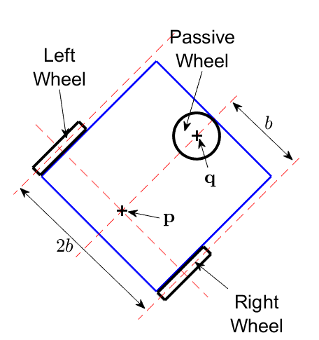
Figure 1: Differential Drive robot diagram.

Now, we consider the DDR, see Fig. 1. This robot has two conventional wheels, of radii $r$, which are actuated by separate motors. The horizontal position of the DDR is determined by the point $\mathbf{p}$ located in the center of the line linking the points of contact of both wheels with the floor. The distance between these points is $2b$. A third unactuated wheel making contact with the floor at point $\mathbf{q}$ provides mechanical stability; it is chosen so that it does not impose any kinematic constraints. The corresponding kinematic model for the DDR is [36]:

$$\left[\begin{array}[]{c}\dot{x}\\ \dot{y}\\ \dot{\theta}\end{array}\right]=\frac{r}{2}\left[\begin{array}[]{cc}\cos(\theta)&\cos(\theta)\\ \sin(\theta)&\sin(\theta)\\ \frac{1}{b}&-\frac{1}{b}\end{array}\right]\left[\begin{array}[]{c}\omega_{R}\\ \omega_{L}\end{array}\right],$$ (2)

where $\omega_{R}\in\mathbb{R}$ and $\omega_{L}\in\mathbb{R}$ are the angular speeds of the right and left wheels, $x$ and $y$ are the $\mathrm{x}$ and $\mathrm{y}$ positions of the DDR, respectively, and $\theta$ is its orientation. The model input vector in (2) is two dimensional, while the DDR configuration (i.e. the output vector) is three dimensional. This implies that the DDR translational velocity (i.e. $[\dot{x},\ \dot{y}]$) and its angular speed $\dot{\theta}$ cannot be controlled independently. The DDR translational speed (i.e. the magnitude of the DDR translational velocity) and its angular speed are expressed as:

$$\left[\begin{array}[]{c}v\\ \dot{\theta}\end{array}\right]=\frac{r}{2}\left[\begin{array}[]{cc}1&1\\ 1&-1\end{array}\right]\left[\begin{array}[]{c}\omega_{R}\\ \omega_{L}\end{array}\right].$$ (3)

Note that while the model (2) is not invertible, the model (3) is invertible. This implies that we can fully set independently the angular speed and translational speed of the robot, but we cannot fully set indpendently its angular speed and its translational velocity.

Another common WMR is the car-like robot. It has two rear conventional wheels which are mechanically coupled to the same motor, and also has two conventional steerable front wheels which are mechanically coupled. Its kinematic model is described in [37].

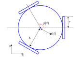
Figure 2: Three-wheeled omnidirectional robot diagram.

Another class of WMR includes omnidirectional robots. They have the particularity of using omnidirectional wheels to enable the robot’s omnidirectional motion, i.e., moving in any direction at any time. One popular MR belonging to this class is the TOMR, see Fig. 2. Its kinematic model is [38]:

$$\left[\begin{array}[]{c}\dot{x}\\ \dot{y}\\ \dot{\phi}\end{array}\right]=r\left[\begin{array}[]{ccc}0&1&L\\ -\sin\left(\frac{\pi}{3}\right)&-\cos\left(\frac{\pi}{3}\right)&L\\ \sin\left(\frac{\pi}{3}\right)&-\cos\left(\frac{\pi}{3}\right)&L\end{array}\right]^{-1}\left[\begin{array}[]{c}\omega_{1}\\ \omega_{2}\\ \omega_{3}\end{array}\right],$$ (4)

where $r$ is the radii of the omnidirectional wheels, $\omega_{i}$ is the angular speed of the $i$th wheel, and $L$ is the distance from the wheels to the robot’s center. Unlike the kinematic models of the DDR and of the car-like robot, that of the TOMR is fully invertible analytically. Hence, we can always independently determine the translational velocity and the angular speed of the MR to find the corresponding exact angular speed of each wheel. Therefore, the TOMR does not present any kinematic restriction on its motion, but dynamic constraints still need to be considered, as will be described in section II-A3.

II-A2 Inverse Kinematic Model

As explained in the previous section, the forward kinematic model is obtained by analysing the MR’s geometry and applying the motion constraints imposed by the wheels. The inverse kinematic models are obtained by inverting the forward kinematic model.

In some cases, the derivation of the inverse kinematic model is straightforward. For instance, consider the kinematic model of the TOMR (4). This is a linear model involving an invertible matrix, and thus the inverse kinematic model for the three-wheeled omnidirectional MR is:

$$\left[\begin{array}[]{c}\omega_{1}\\ \omega_{2}\\ \omega_{3}\end{array}\right]=\frac{1}{r}\left[\begin{array}[]{ccc}0&1&L\\ -\sin\left(\frac{\pi}{3}\right)&-\cos\left(\frac{\pi}{3}\right)&L\\ \sin\left(\frac{\pi}{3}\right)&-\cos\left(\frac{\pi}{3}\right)&L\end{array}\right]\left[\begin{array}[]{c}\dot{x}\\ \dot{y}\\ \dot{\phi}\end{array}\right].$$ (5)

Similarly, the inverse kinematic model for the DDR can be derived from inverting (3):

$$\left[\begin{array}[]{c}\omega_{R}\\ \omega_{L}\end{array}\right]=\frac{b}{r}\left[\begin{array}[]{cc}\frac{1}{b}&1\\ \frac{1}{b}&-1\end{array}\right]\left[\begin{array}[]{c}v\\ \dot{\theta}\end{array}\right].$$ (6)

Finally, some MRs have complex forward kinematic models that are difficult to invert analytically due to nonlinearities and singularities. In such cases, machine learning is a good option for the derivation of the inverse kinematic model [39].

II-A3 Dynamic Model

Dynamic models consider the forces exerted by the robot on its environment. They relate the WMR motion to the torque exerted by each motor and the electric signals producing it. WMR can be modelled as a nonlinear dynamic system whose general form is [40]:

$$\dot{\mathbf{z}}=f(\mathbf{z},\mathbf{u}),$$ (7)

where $\mathbf{z}$ is the state vector of the WMR, where $\mathbf{u}$ is the input signal vector and $f(\cdot)$ is a general function, which can be linear or non-linear. Let us begin the discussion of dynamic models with the popular pure integrator model:

$$\frac{\mathrm{d}^{n}\mathbf{p}(t)}{\mathrm{d}t^{n}}=\mathbf{u}(t),\ \ \ n\in\mathbb{N}^{+},$$ (8)

where $\mathbf{u}$ is the control signal and $\mathbf{p}$ is the WMR position. (8) models a generic omnidirectional robot. It is also a very popular model due to its simplicity, which eases the theoretical analyses. This allows analytical results to be derived with less effort than with the use of more elaborate dynamic models (at the expense of accuracy, however).

Next, we discuss the order $n$ in the model (8). If $n=1$, we obtain the single integrator model, which allows for abrupt velocity changes. This model can describe with some accuracy the WMR motion under any of the following conditions: (i) the WMR speed is constant or changes slowly; (ii) the WMR dynamics is fast enough to follow the input. In [22], the authors used this model to design trajectories, which were then tested experimentally on real WMRs.

The model (8) with $n=2$, which is referred to as the double integrator model, limits the WMR acceleration. It is also a very common model in mobile robotics [5], [41].

The pure integrator model is a very simple general model used to describe a variety of WMRs, but greatly lacks accuracy. We will now begin to discuss more complex and specific dynamic models.

Most WMRs use Direct Current (DC) motors to drive their wheels [36] as they are cheap, easy to control, and efficient. The WMR’s dynamic model can be derived by first modeling the DC motor and then by combining the motor models while considering the MR frame. Following such a procedure, a dynamic model for the DDR is found to be [36]:

$$\dot{\mathbf{z}} = \mathbf{A}\mathbf{z}+\mathbf{B}\mathbf{u},$$ (9)

$$\dot{\mathbf{p}} = \left[\begin{array}[]{ccc}\cos(\phi)&\sin(\phi)&0,\\ 0&0&1,\end{array}\right]^{\mathrm{T}}\mathbf{z},$$ (12)

$$\mathbf{z} = \mathbf{T}_{q}\left[\begin{array}[]{c}\omega_{R}\\ \omega_{L}\end{array}\right],$$ (15)

$$\mathbf{T}_{q}=\frac{r}{2}\left[\begin{array}[]{cc}1&1\\ b^{-1}&-b^{-1}\end{array}\right],$$ (16)

$$\mathbf{p}=[\mathrm{x},\ \mathrm{y},\phi]^{\mathrm{T}},\quad\mathbf{z}=[v,\ \dot{\phi}]^{\mathrm{T}},\quad\mathbf{u}=[u_{R},\ u_{L}]^{\mathrm{T}},$$ (17)

where $u_{R}$ and $u_{L}$ are the normalized input DC voltage to the motors (i.e. $|u_{R}|\leq$$=$$1$ and$|u_{L}|\leq$$=$$1$); $\omega_{R}$ and $\omega_{L}$ are the angular speeds of the right and left wheels, respectively; $\mathbf{p}$ is the pose of the WMR (i.e. the WMR’s horizontal position and orientation); $v$ and $\dot{\phi}$ are the translational speed and the angular speed (around its center) of the WMR, respectively. The matrices $\mathbf{A}$ and $\mathbf{B}$ contain information related to the inertia of the MR, its weight, the friction, the battery voltage level, and other electromechanical parameters of the motors.

From this dynamic model, we observe that: 1) The DDR’s state vector $\mathbf{z}$ is linear w.r.t. the control input $\mathbf{u}$, see (9), but the pose is nonlinear w.r.t. $\mathbf{z}$, see (12). 2) The DDR’s velocity, encoded in $\mathbf{z}$, is related to the input $\mathbf{u}$ by a first-order linear system and its pose is related to $\mathbf{u}$ by a second-order nonlinear system. This implies that the input $\mathbf{u}$ controls the DDR’s acceleration, and so the state $\mathbf{z}$ cannot change abruptly. Consequently, the WMR has the following limitations: (i) it cannot change the speed abruptly, thus requiring a non-zero deceleration time to stop; (ii) it cannot change direction abruptly. 3) If $\dot{\mathbf{z}}$ in (9) is significantly small, then $\mathbf{z}\approx-\mathbf{A}^{-1}\mathbf{B}\mathbf{u}$. In other words, if the DDR’s acceleration is significantly small, then the WMR state $\mathbf{z}$ almost becomes linear w.r.t. the control signal $\mathbf{u}$. As such, the dynamic DDR motion model (9)-(17) does not add additional constraints and can be sufficiently modelled by the kinematic model.

The dynamic model of the TOMR is [32]:

$$\dot{\mathbf{z}} = \mathbf{A}(\phi,\dot{\phi})\mathbf{z}+\mathbf{B}\mathbf{u},$$ (18)

$$\mathbf{p} = \left[\begin{array}[]{cc}\mathbf{I}_{3\times 3}&\mathbf{O}_{3\times 3}\end{array}\right]\mathbf{z},$$ (20)

$$\mathbf{z}=[\mathrm{x},\ \mathrm{y},\phi,\ \dot{\mathrm{x}},\ \dot{\mathrm{y}},\dot{\phi}]^{\mathrm{T}},\quad\mathbf{u}=[u_{1},\ u_{2}\ u_{3}]^{\mathrm{T}},$$ (21)

where:

$$\mathbf{A}(\phi,\dot{\phi})=\left[\begin{array}[]{cc}\mathbf{O}_{3\times 3}&\mathbf{I}_{3\times 3}\\ \mathbf{O}_{3\times 3}&\mathbf{R}(\phi)\dot{\mathbf{R}}^{\mathrm{T}}(\phi)\dot{\phi}-\mathbf{C}\end{array}\right],$$ (22)

$$\mathbf{R}(\phi)=\left[\begin{array}[]{ccc}\cos(\phi)&-\sin(\phi)&0,\\ \sin(\phi)&\cos(\phi)&0,\\ 0&0&1,\end{array}\right].$$ (23)

The matrices $\mathbf{B}$ and $\mathbf{C}$ in (18) and (22) depend on the electromechanical characteristics of the particular TOMR. The matrix $\mathbf{R}(\phi)\dot{\mathbf{R}}^{\mathrm{T}}(\phi)\dot{\phi}$ is related to the Coriolis force.

As opposed to the DDR, where the dynamic model described in (9) is linear, the TOMR dynamic model in (18)-(23) is nonlinear w.r.t. the input. The nonlinearity comes from $\mathbf{A}(\phi,\dot{\phi})$ and, in particular, from the component $\mathbf{R}(\phi)\dot{\mathbf{R}}^{\mathrm{T}}(\phi)\dot{\phi}$ in (21) produced by the Coriolis force. After having discussed some dynamic models for WMRs, we continue with the models for describing their energy consumption due to motion.

II-A4 Energy Consumption model

Most MRs draw their energy from a battery. Due to the limited capacity of the battery, it is important to calculate the MR energy consumption to determine their operation time. There are various approaches to derive energy consumption models, but we will discuss only some of the most common ones.

Electric model: most WMRs use DC motors to actuate their wheels because of their advantages in comparison to other types of motors, as explained in [36]. In this approach, we first calculate the energy consumed by the $k$th motor as a function of the instantaneous electric power:

$$E_{k}=\int_{t}\mathfrak{p}_{k}(t)\mathrm{d}t,$$ (24)

where $\mathfrak{p}_{k}(t)=\mathfrak{i}_{k}(t)\mathfrak{v}_{k}(t)$ is the instantaneous electric power consumed by the $k$th motor, $\mathfrak{i}_{k}(t)$ is the input current, and $\mathfrak{v}_{k}(t)$ is the DC input voltage to the $k$th motor. Since this is a DC motor, the input variable controlling it is the DC input voltage (controlled using Pulse-Width Modulation (PWM)), which is given as:

$$\mathfrak{v}_{k}(t)=u_{k}(t)V_{s},$$ (25)

where $V_{s}$ is the amplitude of the PWM signal and $u_{k}(t)\in[-1,1]$ is the normalized control signal. Circuit theory and electromechanical equations are then used to derive the equations relating the input current $\mathfrak{i}_{k}(t)$ to the angular speed $\omega_{k}$ of the wheel that is mechanically coupled with the motor’s shaft. Thereafter, the dynamic model is used to relate the WMR state vector to the wheel’s angular speed. Finally, these equations are combined to obtain an equation relating the WMR energy consumption to the input vector $\mathbf{u}$ and the WMR state vector. To illustrate this method, we briefly present the energy consumption models of a DDR and of a TOMR. According to [42], the DDR’s energy consumption model is:

$$E = \int_{t}\left(k_{1}\|\mathbf{u}(t)\|^{2}-k_{2}\mathbf{z}^{\mathrm{T}}(t)\mathbf{T}_{q}^{-\mathrm{T}}\mathbf{u}(t)\right)\mathrm{d}t,$$ (26)

where the integrand corresponds to the electric power consumed and the parameters $k_{1}$ and $k_{2}$ depend on electromechanical properties of the motors. Variables $\mathbf{u}$, $\mathbf{z}$, and $\mathbf{T}_{q}$ have the same definition as in (9)-(17). The energy consumption model for the three-wheeled omnidirectional MR is given in [32] as:

$$E = \int_{t}\left(k_{1}\|\mathbf{u}(t)\|^{2}-k_{2}\dot{\mathbf{p}}^{\mathrm{T}}(t)\mathbf{R}(\phi)\mathbf{B}\mathbf{u}(t)\right)\mathrm{d}t,$$ (27)

where $\mathbf{u}(t)$, $\mathbf{p}(t)$, and $\mathbf{B}$ have the same definition as in (18), while $k_{1}$ and $k_{2}$ depend on the motor’s electromechanical characteristics. In [43], the authors present an energy consumption model for a car-like robot derived using the same method, however neglecting the energy required to steer.

This model describes the electrical energy consumed at the input of the motors and takes into account the energy lost as heat within the motor. (26) and (27) are quadratic functions of the normalized control signal $\mathbf{u}(t)$.

Physics approach: another approach to describe the WMR energy consumption is to analyze the system from an external perspective and calculate the WMR’s kinetic energy and the energy required to overcome the floor’s friction. To illustrate this type of model, let us consider the energy consumption model of the DDR presented in [44]:

$$E_{\rm motors}=E_{\rm kin}+E_{\rm res},$$ (28)

where $E_{\rm kin}$ is the kinetic energy, $E_{\rm res}$ is the energy consumed by the motors to overcome the traction resistance presented by the friction of the floor, and $E_{\rm motors}$ is the energy consumed by the motors, which is measurable from an external point of view, i.e., without taking into account the internal losses. The kinetic energy is given by:

$$E_{\rm kin} = \frac{1}{2}mv^{2}(t)+I\omega^{2}(t),$$ (29)

$$= \int_{t}\{mv(t)a(t)+I\omega(t)\beta(t)\}\mathrm{d}t,$$

where $m$ is the total WMR’s mass; $I$ is the total WMR’s rotational inertia; $v$ and $\omega$ are the translational and rotational speeds, respectively; and $a(t)$ and $\beta(t)$ are the translational and rotational accelerations, respectively. The products $v(t)a(t)$ and $\omega(t)\beta(t)$ in (29) can be negative when the WMR stops, meaning that the WMR’s motors get some power back that could be recovered by the WMR’s electrical system. But, most WMR’s do not have the electric systems to recover such power and thus, considering this limitation, (29) becomes:

$$E_{\rm kin}=\int_{t}\{m\max(v(t)a(t),0)+I\max(\omega(t)\beta(t),0)\}\mathrm{d}t.$$ (30)

The term describing the energy consumed to overcome friction in (28) is:

$$E_{res}=2\mu mg\int_{t}\max(|v(t)|,b|\omega(t)|)\mathrm{d}t.$$ (31)

The distance travelled by the DDR is approximately $\int_{t}|v(t)|\mathrm{d}t$. The advantage of this model lies with its independence to the type of motor used by the WMR. It requires only the mass $m$ and the rotational inertia $I$ of the WMR, which can be estimated. The disadvantage is that it only considers the energy expenditure observed from the outside and does not take into account the internal losses of the motors and the circuitry.

Data-driven Model: the energy consumption models mentioned above are derived from physical principles. Those theoretical models, for the sake of tractability, often ignore certain effects, such as nonlinearities of the motor or the influence of temperature on the electric resistances. Another approach consists of measuring the electric consumption of the WMR under different conditions, creating a dataset, and then training numerical models. The authors of [45] present a simple implementation of this approach by measuring the power consumed by DC motors at different angular speeds. The authors note that a suitable model for the power consumption of the $k$th motor is:

$$P_{k}=\sum_{j=0}^{6}a_{j}\omega_{k}^{j},$$ (32)

where $\omega_{k}$ is the angular speed of the $k$th motor and $\{a_{j}\}_{j=0}^{6}$ are experimentally determined coefficients. The model in (32) is then combined with the kinetic model, which relates the velocity of the WMR to the angular speed of the wheels $\omega_{k}$ in order to obtain the power consumed by the WMR. After integration over time, we obtain the consumed energy.

In [46], there are two examples of this type of energy consumption model. First, the authors measure the power consumption of the PPRK (a commercial TOMR moving at a constant linear speed $v$. The measurements are done at different linear speeds up to a maximum value. After a numerical analysis of the measurements, the authors observed that the power consumed by the PPRK can be well-modelled by a fourth order polynomial function of the linear speed. Next, the authors did the same for the Pioneer 3DX (a commercial DDR) and measured its energy consumption while moving at a constant speed on a straight line. Due to limitations in the robot’s internal system, the Pioneer 3DX could not be operated at its maximum linear speed. The experimental results showed that the power consumption of this robot can be modelled with an affine function of the linear speed.

The derivation of this type of model can require significant time to gather data in the laboratory. Additionally, the generalisation of the derived models to conditions different from those of the modeling phase might exhibit an uncertain accuracy, e.g. when trying to use the model in [46] to predict the energy consumption of the Pioneer 3DX while moving along curves or at variable linear speed. On the other hand, one advantage of this type of model is that they do not require deep theoretical knowledge. Also, they can implicitly consider the various complex processes involved in energy consumption, which may be complicated to take into account in the theoretical models. For example in [45], the authors mention that DC motors can be modelled with a second-order polynomial of the angular speed $\omega$ from electromagnetic theory. Yet, measurements show that such a model is insufficient. For example, the sixth-order polynomial model introduced in (32) exhibited a much better fit on real measurements. This may be due to the fact that the second-order model derived from theory overlooks certain processes, while the model in (32) took them into account implicitly through the fitting process.

Restricted Domain Models: some simple energy consumption models are derived from more complex models by constraining their range of validity. To illustrate this, let us consider the work in [47] where the authors use an electric energy consumption model for a DDR, similar to the one used in (26). They restrict the DDR to move within a straight line with a trapezoidal linear speed profile. For such a trajectory, they analytically calculate the energy consumption starting from the electric energy consumption model to obtain the following expression:

$$E=\sum_{j=-1}^{3}a_{j}\omega^{j},$$ (33)

where $\omega$ is the angular speed of the DDR wheels. The model (33) exposes an interesting phenomenon that is sometimes overlooked: motors can be inefficient when operated at very low speeds. As the motor’s speed decreases, the term $\omega^{-1}$ in (33) dominates the energy consumption and grows very quickly. After the optimization of the trapezoidal speed profile, the authors found that the energy consumption is proportional to the distance travelled when the total duration of movement remains constant. Based on the result in (33), the authors of [48] modeled the energy consumption as being proportional to the distance $D$ travelled by the WMR:

$$E=kD,$$ (34)

where $k$ is a proportionality factor. The model (34) has been adopted by many authors for simplicity and is sometimes derived in a similar manner in different papers, or sometimes just assumed as it is intuitive and simple, see [49] and [50].

These models are, in general, simplifications of other more complex models under certain conditions. When choosing a model, we must consider where it comes from and how it was derived in order to see if the application in which we intend to use it is close enough to the conditions under which the model was derived. This is done so as to ensure that we do not operate the model outside its range of validity. Otherwise, if we neglect this aspect, then the model selected might deviate significantly from the true energy consumption. For example, while the model introduced in (34) is appropriate when a WMR is moving at a constant speed, it may be quite inaccurate when the speed varies considerably over time.

Square norm: lastly, another popular energy consumption model within the control theory community is :

$$E=\int_{0}^{t}\|\mathbf{u}(\tau)\mathrm{d}\|^{2}\tau,$$ (35)

where $\mathbf{u}$ is the control signal of the WMR dynamic model. This is notably a simplification of the energy consumption models derived through circuit theory presented in (26) and (27). The model in (35) becomes closer to the models (26) and (27) when the WMR operates at low speeds and/or the coefficient $k_{2}$ of those models is small. ∎

Although motion consumes a significant part of the energy in WMRs, there are also other processes which consume a non-negligible amount of energy. In [51], the authors empirically evaluated the contribution of different processes to the energy consumption of a DDR and found that the sensors and microcontrollers also contribute significantly to energy consumption The microcontroller’s power consumption can be modelled as constants, since they usually perform low level tasks which are repetitive and relatively stable. On the other hand, the power consumption of the embedded computers can be modelled as a stochastic process as they usually perform tasks which depend more on exogenous inputs, and thus have a more variable behaviour.

II-B Rotary-wing UAVs

The study of the motion of aerial vehicles is a complex subject that has been investigated since the early appearance of the first airplanes. There is a large body of literature on the aerodynamic aspects of these vehicles and their modeling. In this section, we will discuss the quadrotor aerial robot, which is a basic type of multirotor UAV.

Multirotor aerial robots (also called rotary-wing aerial robots) are one of the most popular types of aerial robots nowadays. One of the most common type of these UAVs is the quadrotor, which is the subject of this section.

The WMRs discussed in the previous section operate in 2D and their configuration is fully described by their horizontal position and orientation. In contrast, UAVs operate in 3D. To fully describe their configuration, we need to specify their 3D position, as well as their attitude, which can be expressed using either Euler angles or quaternions [52, 53]. In this tutorial, we will limit the discussion to models representing the attitude using Euler angles; details about the utilisation of quaternions to represent the attitude can be found in [54].

The configuration of the UAV can be described using Euler angles as:

$$\mathbf{p}(t)=[x,\ y\ ,z,\ \theta,\ \phi,\ \psi]^{\mathrm{T}},$$ (36)

where $[x,\ y\ ,z]^{\mathrm{T}}$ is the UAV center of mass and $\theta$, $\phi$, and $\psi$ are the Euler angles of roll, pitch, and yaw, respectively, which describe the orientation of the UAV (see [55] for a more detailed geometrical description of these angles). Note that $[x,\ y\ ,z]^{\mathrm{T}}$ is represented in a static coordinate frame attached to the world and not to the UAV itself, and $[\theta,\phi,\psi]^{\mathrm{T}}$ are represented in a coordinate frame attached to the center of mass of the UAV oriented in the same manner as the inertial coordinate frame. Before discussing the quadrotor dynamic model, we will briefly discuss the physical principles that allow it to fly. In a classic quadrotor, the four propellers lie in the same plane and are oriented vertically. When the propeller rotates, it creates thrust in the same direction as its orientation and with a sense opposing the gravity. The faster the propeller turns, the greater the thrust generated. When all four propellers produce the same thrust, the plane containing all four propellers is parallel to the floor, and the resulting thrust is vertical. If this thrust equals the gravitational force, then the quadrotor remains in the air hovering. When one propeller turns faster or slower than the other, the quadrotor tilts and the resulting thrust presents a horizontal component, making the UAV move in the horizontal plane.

Just as the dynamic models of the WMRs were derived starting from the electrical analysis of their motors, the derivation of the dynamic model for multirotors begins in the same way. Consider a dynamic model for the quadrotor that is used by many roboticists [56]:

$$\left[\begin{array}[]{c}\frac{\mathrm{d}^{{2}}{\mathsf{x}}}{\mathrm{d}{t}^{{2}}}\\ \vskip 3.0pt plus 1.0pt minus 1.0pt\cr\frac{\mathrm{d}^{{2}}{\mathsf{y}}}{\mathrm{d}{t}^{{2}}}\\ \vskip 3.0pt plus 1.0pt minus 1.0pt\cr\frac{\mathrm{d}^{{2}}{\mathsf{z}}}{\mathrm{d}{t}^{{2}}}\end{array}\right] = \left[\begin{array}[]{c}\mathrm{c}(\phi)\mathrm{s}(\theta)\mathrm{c}(\psi)+\mathrm{s}(\phi)\mathrm{s}(\psi)\\ \vskip 3.0pt plus 1.0pt minus 1.0pt\cr\mathrm{c}(\phi)\mathrm{s}(\theta)\mathrm{s}(\psi)-\mathrm{s}(\phi)\mathrm{c}(\psi)\\ \vskip 3.0pt plus 1.0pt minus 1.0pt\cr\mathrm{c}(\phi)\mathrm{c}(\theta)\end{array}\right]\frac{{u}_{\mathsf{z}}}{m}-\left[\begin{array}[]{c}0\\ 0\\ g\end{array}\right],$$ (46)

$$\left[\begin{array}[]{c}\frac{\mathrm{d}^{{2}}{\phi}}{\mathrm{d}{t}^{{2}}}\\ \vskip 3.0pt plus 1.0pt minus 1.0pt\cr\frac{\mathrm{d}^{{2}}{\theta}}{\mathrm{d}{t}^{{2}}}\\ \vskip 3.0pt plus 1.0pt minus 1.0pt\cr\frac{\mathrm{d}^{{2}}{\psi}}{\mathrm{d}{t}^{{2}}}\end{array}\right] = \left[\begin{array}[]{c}\left(\frac{I_{\mathsf{y}}-I_{\mathsf{z}}}{I_{\mathsf{x}}}\right)\,\frac{\mathrm{d}{\theta}}{\mathrm{d}{t}}\,\frac{\mathrm{d}{\psi}}{\mathrm{d}{t}}-\frac{J}{I_{\mathsf{x}}}\,\frac{\mathrm{d}{\theta}}{\mathrm{d}{t}}\,{q}_{w}\\ \vskip 3.0pt plus 1.0pt minus 1.0pt\cr\left(\frac{I_{\mathsf{z}}-I_{\mathsf{x}}}{I_{\mathsf{y}}}\right)\,\frac{\mathrm{d}{\phi}}{\mathrm{d}{t}}\,\frac{\mathrm{d}{\psi}}{\mathrm{d}{t}}+\frac{J}{I_{\mathsf{y}}}\,\frac{\mathrm{d}{\phi}}{\mathrm{d}{t}}\,{q}_{w}\\ \vskip 3.0pt plus 1.0pt minus 1.0pt\cr\left(\frac{I_{\mathsf{x}}-I_{\mathsf{y}}}{I_{\mathsf{z}}}\right)\,\frac{\mathrm{d}{\phi}}{\mathrm{d}{t}}\,\frac{\mathrm{d}{\theta}}{\mathrm{d}{t}}\end{array}\right]+\left[\begin{array}[]{c}\frac{\ell\,{u}_{\mathsf{y}}}{I_{\mathsf{x}}}\\ \vskip 3.0pt plus 1.0pt minus 1.0pt\cr\frac{\ell\,{u}_{\mathsf{x}}}{I_{\mathsf{y}}}\\ \vskip 3.0pt plus 1.0pt minus 1.0pt\cr\frac{\,{u}_{\psi}}{I_{\mathsf{z}}}\end{array}\right],$$ (57)

$$\left[\begin{array}[]{c}{u}_{\mathsf{x}}\\ {u}_{\mathsf{y}}\\ {u}_{\mathsf{z}}\\ {u}_{\psi}\end{array}\right] = \left[\begin{array}[]{cccc}-\kappa_{b}&0&\kappa_{b}&0\\ 0&\kappa_{b}&0&-\kappa_{b}\\ \kappa_{b}&\kappa_{b}&\kappa_{b}&\kappa_{b}\\ \kappa_{\tau}&-\kappa_{\tau}&\kappa_{\tau}&-\kappa_{\tau}\end{array}\right]\left[\begin{array}[]{c}{\omega}_{1}^{2}\\ {\omega}_{2}^{2}\\ {\omega}_{3}^{2}\\ {\omega}_{4}^{2}\end{array}\right],$$ (71)

$${q}_{w} = \omega_{1}-\omega_{2}+\omega_{3}-\omega_{4},$$ (73)

where ${u}_{\mathsf{x}}(t)$, ${u}_{\mathsf{y}}(t)$, ${u}_{\mathsf{z}}(t)$, and ${u}_{\psi}(t)$ denote the control signals for the drone; $\omega_{j}(t)$ is the angular velocity of the $j$th motor; $m$ is the total mass of the drone; $g$ is the gravitational constant; $\ell$ is the distance from the center of the quadrotor to each motor; $I_{\mathsf{x}}$, $I_{\mathsf{y}}$, and $I_{\mathsf{z}}$ are the rotational inertia components; $J$ is the total inertia of the motors; and $\kappa_{b}$ and $\kappa_{\tau}$ are the thrust and aerodynamic drag factors of the propellers, respectively. In (71), the matrix relating the vector inputs $\left[\begin{array}[]{cccc}{u}_{\mathsf{z}}&{u}_{\mathsf{y}}&{u}_{\mathsf{x}}&{u}_{\psi}\end{array}\right]^{T}$ with the square angular velocities vector $\left[\begin{array}[]{cccc}{\omega}_{1}^{2}(t)&{\omega}_{2}^{2}(t)&{\omega}_{3}^{2}(t)&{\omega}_{4}^{2}(t)\end{array}\right]^{\mathrm{T}}$ is not singular.

Equation (57) describes the drone’s Euler angles (roll $(\phi)$, pitch $(\theta)$, and yaw $(\psi)$) measured with respect to the axes $o_{B}{\mathsf{x}}_{B}$, $o_{B}{\mathsf{y}}_{B}$, and $o_{B}{\mathsf{z}}_{B}$, with $(o_{B}{\mathsf{x}}_{B}{\mathsf{y}}_{B}{\mathsf{z}}_{B})$ being the body axis system whose origin ${o_{B}}$ is given by the geometric centre of the quadrotor.

The quadrotor motion given by the model in (46)-(73) is described w.r.t. to a fixed orthogonal axis set ${(o{\mathsf{x}}{\mathsf{y}}{\mathsf{z}})}$, where ${o{\mathsf{z}}}$ points vertically up, i.e. opposed to the gravity vector. The origin ${o}$ is located at a desired height ${\bar{\mathsf{z}}}$ with respect to the ground level. The coordinates $\mathsf{x}$, $\mathsf{y}$, and $\mathsf{z}$ in (46) refer to the position of the centre of gravity of the quadrotor in the space where $\mathsf{z}$ is its altitude [57]. In the literature, we find different axis configurations in which the quadrotor motion can be described and each axis configuration provides slightly different models. The time dependence of the variables in equations (46) and (57) is not explicitly shown in order to lighten the notation. Further, due to the symmetry of the quadrotor, we have $I_{\mathsf{x}}=I_{\mathsf{y}}=I$.

More complex models are also possible, which consider external disturbances, such as the wind. Regarding the energy consumption of the quadrotor, there are electric models and physics-based models that are derived using approaches similar to those used for the WMR. In [56], the energy consumption of a quadrotor is modeled as:

$$E = \sum_{j=1}^{4}\int_{t}\Bigg{[}\left(\sum_{k=0}^{4}c_{k}\omega_{j}^{k}(t)\right)+c_{6}\dot{\omega}_{j}(t)+c_{7}\dot{\omega}_{j}^{2}(t)$$ (74)

$$+ c_{8}\omega_{j}(t)\dot{\omega}_{j}(t)+c_{9}\omega_{j}^{2}(t)\dot{\omega}(t)\Bigg{]}\mathrm{d}t,$$

where the coefficients $\{c_{k}\}_{0}^{9}$ depend on the parameters of the quadrotor’s motors and the geometry of the propellers.

In [58], the authors present the following hybrid energy consumption model based on basic mechanics and completed with some correction factors obtained experimentally:

$$E_{c} = \int_{t_{0}}^{t_{f}}\sum_{j=1}^{4}\tau_{j}(t)\omega_{j}(t)\mathrm{d}t,$$

$$= \int_{t_{0}}^{t_{f}}\sum_{j=1}^{4}\left(\dot{\omega}_{j}(t)+\mathcal{K}_{\tau}\omega_{j}^{2}(t)+D_{v}\omega_{j}(t)\right)\omega_{j}(t)\mathrm{d}t,$$

where (II-B) is the energy consumed by the four motors of the quadrotor. In other words, (II-B) only describes the amount of energy that is translated into mechanical energy, but disregards the efficiency of the motors.

II-C Fixed-wing UAVs

In this section, we briefly discuss fixed-wing UAVs and present a simple, but useful dynamic model for CaTP problems. Fixed-wing UAVs fly using principles that are different from those used by multirotor UAVs and are consequently modelled in a different manner with different characteristics.

In general, fixed-wing UAVs are more energy-efficient than multirotor UAVs mainly because of their ability to glide. They also fly for longer times, longer distances, and at higher speeds. However, they are less agile and cannot land or take-off vertically. As opposed to multirotor UAVs, fixed-wing UAVs are generally not designed to hover. Nevertheless, some special types of fixed-wing UAVs having high thrust-to-weight ratios can hover using complex control techniques [59].

Fixed-wings UAV are controlled by the thrust generated by its propeller(s) and by controlling surfaces (aileron, elevator, and rudder). Micro fixed-wing UAVs usually drive their propellers with an electric motor, while small fixed-wing UAVs can drive it using gas powered motors.

The fixed-wing UAV center of mass position is sometimes described in the North-East-Down (NED) coordinate system, where the down axis points towards the center of the Earth and is aligned with the force of gravity. In this case, the altitude is measured in the opposite direction of the down axis. The attitude of the fixed-wing airplane is expressed using Euler angles in the body frame defined as follows: its origin lies in the center of gravity of the airplane, the $x$ axis points to the nose of the plane, the $y$ axis points to the right wing, and the $z$ axis is orthogonal to those two axes and follows the right-hand rule. The roll $\phi$ describes the rotation about the $x$ axis, the pitch $\theta$ describes the rotation about the $y$ axis, and the yaw $\psi$ describes the rotation about the $z$ axis.

The aerodynamics of airplanes are significantly more complex and nonlinear. Since this is an elementary tutorial, we will present only a high-level simplified dynamic model that can be used for trajectory planing, as well as one linearized dynamic model. In the absence of wind, a simplified nonlinear dynamic model describing the fixed-wing UAV motion is [60]:

$$\left[\begin{array}[]{cc}\dot{p}_{n}\\ \dot{p}_{e}\\ \dot{h}\end{array}\right]=V_{a}\left[\begin{array}[]{cc}\cos(\psi)\cos(\gamma)\\ \sin(\psi)\cos(\gamma)\\ \sin(\gamma)\end{array}\right]$$ (76)

$$\left[\begin{array}[]{cc}\dot{\psi}\\ \dot{\gamma}\end{array}\right]=\left[\begin{array}[]{cc}\frac{F_{lift}}{mV_{a}}\frac{\sin(\phi)}{\cos(\gamma)}\\ \frac{F_{lift}}{mV_{a}}\cos(\phi)-\frac{g}{V_{a}}\cos(\gamma)\end{array}\right]$$ (77)

$$\left[\begin{array}[]{cc}F_{lift}\\ F_{drag}\end{array}\right]=\frac{1}{2}\rho V_{a}^{2}S\left[\begin{array}[]{cc}C_{L}\\ C_{D_{0}}+KC_{L}^{2}\end{array}\right]$$ (78)

$$\dot{V}_{a}=\frac{F_{\rm thrust}}{m}-\frac{F_{\rm drag}}{m}-g\sin(\gamma)$$ (79)

where $g$ is the gravitational constant, $S$ is the planform area of the wing, $C_{D_{0}}$ is the zero lift drag, $K$ is the induced drag factor, $m$ is the mass of the airplane, and $\rho$ is the air density. The input to this model is the lift coefficient $C_{L}$, the thrust $F_{\rm thrust}$, and the roll $\phi$. $\dot{p}_{n}$ and $\dot{p}_{e}$ are the speeds along the north and east axes, respectively, and $\dot{h}$ is the altitude speed measured w.r.t. to the negative direction of the down axis. $F_{lift}$ and $F_{\rm drag}$ are the lift and drag forces experienced by the plane. Finally, $V_{a}$ is the air speed of the airplane.

The constant altitude and the airspeed scenario (i.e. $\dot{h}=0$ and $\dot{V}_{a}=0$) are common and of particular importance for CaTP applications. In this case, we have $\gamma=0$, $\dot{\gamma}=0$, and $F_{thrust}=F_{drag}$. The dynamic model (76)-(79) reduces to the kinematic model:

$$\left[\begin{array}[]{cc}\dot{p}_{n}\\ \dot{p}_{e}\end{array}\right]=V_{a}\left[\begin{array}[]{cc}\cos(\psi)\\ \sin(\psi)\end{array}\right]$$ (80)

$$\dot{\psi}=({g}/{V_{a}})\tan(\phi).$$ (81)

With this kinematic model, the paths are usually composed of straight lines and circular arcs [61]. The simplified models (76) and (80) are practical, but they do not describe the pitch angle $\theta$. This can be an issue for some CaTP since the variations in the orientation of the antenna mounted on the fixed-wing UAV cannot be fully determined without the pitch $\theta$.

Another simple type of dynamic model for the fixed-wing UAV are the linear models. These models are derived after linearizing more complex nonlinear aerodynamic models around small attitude variations. They are separated into two decoupled models, the longitudinal motion model and the lateral motion model. The longitudinal motion model is:

$$\left[\begin{array}[]{c}\dot{u}\\ \dot{w}\\ \dot{q}\\ \dot{\theta}\\ \dot{h}\end{array}\right]=\mathbf{A}\left[\begin{array}[]{c}u\\ w\\ q\\ \theta\\ h\end{array}\right]+\mathbf{B}\left[\begin{array}[]{c}\delta_{e}\\ \tau\end{array}\right]$$ (94)

where $\tau$ is the thrust and $\delta_{e}$ is the elevator angle. For the lateral model, we have that:

$$\left[\begin{array}[]{c}\dot{v}\\ \dot{p}\\ \dot{r}\\ \dot{\phi}\\ \dot{\psi}\end{array}\right]=\mathbf{C}\left[\begin{array}[]{c}v\\ p\\ r\\ \phi\\ \psi\end{array}\right]+\mathbf{D}\left[\begin{array}[]{c}\delta_{a}\\ \delta_{r}\end{array}\right]$$ (107)

where $\delta_{a}$ and $\delta_{r}$ are the action of the aileron and the rudder, respectively. The matrices $\mathbf{A}$, $\mathbf{B}$, $\mathbf{C}$, and $\mathbf{D}$ depend on the particular airplane. Since this is an elementary tutorial, we did not consider the effect of wind on the fixed-wing UAV motion models, but the interested reader can look into [62, 63, 64, 65] for more information regarding this subject.

It can be demonstrated from physical principles that the energy consumption for the fixed-wing UAV can be expressed as follows [10]:

$$E = \int_{0}^{T}\left(c_{1}\|\mathbf{v}\|^{3}+\frac{c_{2}}{\|\mathbf{v}\|}\left(1+\frac{\|\mathbf{a}\|^{2}-\frac{\mathbf{a}^{T}\mathbf{v}}{\|\mathbf{v}\|^{2}}}{g^{2}}\right)\right)\mathrm{d}t$$ (108)

$$+ \frac{m}{2}(\|\mathbf{v}\|^{2}(T)-\|\mathbf{v}\|^{2}(0))$$

where $\mathbf{v}$ is the velocity and $\mathbf{a}$ is the acceleration of the UAV.

II-D Final Comments on Models for Robots

We have presented an overview of some relevant MR’s models that are useful for CaTP problems, but have omitted some important observations. The models presented in this section are all in continuous time, but it is possible to transform them into discrete time models by transforming differential equations into difference equations. Continuous-time models allow for the utilisation of many analytical tools based on derivatives, such as calculus of variations. On the other hand, discrete-time models allow for numerical techniques like dynamic programming or other related techniques. It is important to mention that, in practice, the control signals for the ground MRs and the UAVs are executed in digital computers on board, and thus the control system is implemented in discrete time.

Finally, all the kinematic and dynamic models described in this section are analytical and are mostly derived from physics. But, there are other types of motion models derived through experimentation and machine learning techniques [66].

III Communications System

This section mainly addresses researchers who desire to work on CaTP, but lack the background in communications systems. Those familiar with the topic can skip this section and directly proceed to section IV. In this section, we introduce the reader to the basic concepts of communication systems and wireless channel models required to study CaTP problems. We begin by introducing a common communication system: transceiver. This is a device composed of a transmitter and a receiver. When a communications link is established between two entities, it can take three different forms:

Simplex Link: one entity operates exclusively as a transmitter and the other operates exclusively as a receiver. The data flow is always unidirectional.

Full-Duplex Link: both entities receive and transmit simultaneously. Two independent data flows in opposite directions occur simultaneously.

Half-Duplex Link: both entities receive and transmit in turns, where two independent data flow in opposite directions, but only one is active at a time. This can be implemented using time duplexing, where during an interval of time, one entity transmits and the other receives. During the next interval of time, the roles are swapped. This is periodically repeated. ∎

We now provide a brief overview of the digital transmission. The source node generates data as blocks of bits or as a continuous stream of bits. This data is then divided in small groups, which are inserted into packets to form the payload. Each packet has a header that contains information such as the destination and/or checkup bits to evaluate the integrity of the packet at the receiver. There are two main strategies to exploit the checkup bits in the packet’s header:

Retransmission: if the receiver does not detect any error in the received data packet, it transmits a confirmation packet back to the source node (containing no payload), indicating that the data packet was correctly received. Thereafter, the source node can transmit new data packets (containing new payload). However, if the receiver detects an error in the received data packet, it does not send back the confirmation packet. When the source node realizes that it did not receive a confirmation packet, it assumes that an error occurred and re-transmits the same data packet. The number of retransmissions will depend on the particular communications protocol.

No-retransmission: if the receiver detects an error in the data packet, it discards the payload. On the other hand, if the packet is correctly received, the receiver does not transmit any confirmation to the source node and simply waits for the next packet. The source node continues to transmit data packets. ∎

The retransmission strategy provides robustness to the transmission of data at the cost of a lowered bit rate and increased latency due to the time spent in confirmation and retransmission of data packets. The no-retransmission strategy can achieve a higher bit rate and lower latency at the cost of more erroneous or missing data. The selection of the transmission strategy will depend on the particular application requirements.

After forming the packets, the transmitter modulates the sequence of bits with a carrier signal of high frequency $f_{c}$ (or equivalently of short wavelength $\lambda\triangleq c/f_{c}$ where $c$ is the speed of light) suitable to be radiated as an electromagnetic waves, which are then radiated through the antenna. The propagation environment modifies the radiated wave before arriving to the receiver’s antenna, where it is converted back to an electric signal and processed. The wireless channel model describes the effect that the propagation environment has on the transmitted signal until it reaches the receiver.

III-A Wireless channel modelling

In the context of CaTP, oversimplified wireless channel models can lead the designer to overestimate the communications channel quality and to overlook certain channel behaviours that the MR will encounter in real conditions. In such cases, the MR might underperform or fail to complete its task due to unexpectedly poor communication quality.

To provide the researcher with the basic knowledge of communications for CaTP problems, we will limit the discussion to the simplest type of communications systems: narrowband, single-antenna, and single carrier communications systems. In addition, we will not address the issue of interference. The general channel model representing such systems is:

$$y(t)=\mathcal{H}(\mathbf{p}(t),\mathbf{q}(t),t)x(t)+n(t),$$ (109)

where $x(t)$ and $y(t)$ are the continuous-time transmitted and received complex signals, respectively; $n(t)$ is the noise generated at the receiver, which is usually modelled as a random complex circular white Gaussian process; $\mathbf{p}(t)$ and $\mathbf{q}(t)$ are the positions of the transmitter and the receiver, respectively, at time $t$; and $\mathcal{H}(\mathbf{p}(t),\mathbf{q}(t),t)$ is the complex channel gain. CaTP problems require models that describe the spatio-temporal channel gain $\mathcal{H}(\mathbf{p}(t),\mathbf{q}(t),t)$. We further discuss different common models to describe the spatial variations of the channel gain. To model $\mathcal{H}(\mathbf{p}(t),\mathbf{q}(t),t)$, deterministic, stochastic, and machine learning approaches can be used.

III-A1 Deterministic Models

In the deterministic approach [67], the wireless channel models are often derived from physical principles. One of the simplest and yet most important channel models is the power loss model. It is the base for many more sophisticated channel models and describes how the mean received signal power varies with the transmitter-receiver distance. It is modelled as [68]:

$$\mathcal{H}(\mathbf{p}(t),\mathbf{q}(t),t)=L_{P}^{-1}(\mathbf{p}(t),\mathbf{q}(t)),$$ (110)

$$L_{P}(\mathbf{p}(t),\mathbf{q}(t))=K_{0}\left({\|\mathbf{q}(t)-\mathbf{p}(t)\|_{2}}/{d_{0}}\right)^{\alpha/2},$$ (111)

where $\alpha$ is the power path loss coefficient, $d_{0}$ is a reference distance, and $K_{0}$ is the path loss observed at distance $d_{0}$ that must be in the far field region [69]. This model is valid for distances larger than $d_{0}$, and is used at distances larger than the radiated signal’s wavelength and the physical antenna’s dimensions [67]. Under free space conditions, the power path loss coefficient becomes $\alpha=2$, but experimental results have reported path loss coefficients as low as $\alpha=1.6$ [70, 71] in some urban environments, buildings, and underground mines. This occurs because some hallways and tunnels behave as giant waveguides due to their geometry and the presence of metallic objects that act as reflectors.

Experiments have shown that the power path loss coefficient can change after certain distances. This is modelled using break points [70] after which the path loss changes.

Another deterministic extension to the model in (111) is the two-ray model [68], which takes into consideration only the Line of Sight (LoS) wave and the wave that reaches the receiver’s antenna after only one reflection on the floor. This model was originally derived in the context of cellular network communications [72]. It has been tested for scenarios with a transmitter of less than 50m altitude; this model makes the assumption that the distance between the transmitter and the receiver is such that the curvature of the earth can be neglected, and thus the floor is considered flat.

If we consider multiple waves beside the LoS and the reflected wave of the two-ray channel model, then we obtain the ray tracing model [73], [74], [75]. This method determines the interaction of multiple radiated waves with the environment (e.g. buildings, floor, walls) before arriving to the receiver’s antenna and requires a computational map of the area in which both the transmitter and the receiver operate. The accuracy of the ray tracing model increases when the map is more detailed and when more electromagnetic interactions are considered (e.g. reflection, refraction, diffraction). However, this also increases the computational load.

Let us discuss another deterministic channel model which has been specially devised for indoor operations, and which also requires a map of the building as well as the positions of both transceivers. This model draws a straight line between both nodes, counts the number of walls and floors crossed [76], and then represents the losses due to those walls and floors as described in [77].

III-A2 Stochastic Models

Stochastic models describe the channel in terms of its mean, variance, and correlation functions, rather than trying to predict the exact channel value, unlike deterministic models. Stochastic models are usually simple and can describe the average behaviour of the channel models accurately as well as its statistics. Their simplicity allows for mathematical analysis that can provide useful insights in many application domains, including CaTP problems. Using this approach, $\mathcal{H}(\mathbf{p}(t),\mathbf{q}(t),t)$ is modelled as a multi-scale spatial and time-varying stochastic process [78] composed of three terms [78, 79]:

$$\mathcal{H}(\mathbf{p}(t),\mathbf{q}(t),t) = \frac{s(\mathbf{p}(t),\mathbf{q}(t))h(\mathbf{p}(t),\mathbf{q}(t),(t))}{L_{P}(\mathbf{p}(t),\mathbf{q}(t))},$$ (112)

where $s(\mathbf{p}(t),\mathbf{q}(t))$ represents the shadowing [80, 81], $h(\mathbf{p}(t),\mathbf{q}(t),t)$ represents the small-scale fading [69], and $L_{P}(\mathbf{p}(t),\mathbf{q}(t))$ represents the path loss [68]. We proceed to discuss the physical meaning of these components and their most relevant mathematical models from the perspective of CaTP applications.

Path-loss: this describes a deterministic component that models the mean power loss variations due to distance between the transmitter and the receiver. It usually takes the form of (111). There are also experimentally derived models for the path loss models, such as the Okumura-Hata model [82].

Shadowing: this is a random process that models the signal power reduction due to obstructions caused by large objects, such as buildings. It is a time-invariant term and depends on the transmitter and receiver positions. The shadowing has been experimentally characterized [80] and is generally modelled as a log-normal real random process with variance $\sigma$ and mean $\mu$. Its spatial autocorrelation has been found experimentally to follow an exponential function [78]:

$$r({d}(t))=\exp\left(-d(t)/\beta\right),$$ (113)

where $\beta$ is the decorrelation distance that is usually in the order of $10\lambda$, and is thus also called large-scale fading. For small distances (smaller than $\beta$), the shadowing is often considered constant. To give more flexibility to the shadowing model, $\sigma$ and mean $\mu$ can be made dependent on the geographical region [79]. The shadowing effect can thus be simulated numerically using mathematical models [84].

Multipath-fading: the electromagnetic wave radiated by the transmitter reaches the receiver’s antenna after travelling through multiple random paths. These multiple components interact with the environment through reflection, diffraction, and refraction before arriving, with different phases, to the receiver’s antenna where they are combined. As a consequence, the receiver observes constructive interference in some locations and destructive interference in others. This results in a random spatial process with large signal strength variations over small distances (smaller than $1\lambda$). This phenomenon is called small-scale fading or multi-path fading [67, 85].

Small-scale fading $h(\mathbf{p}(t),\mathbf{q}(t),t)$ is modelled as a random spatial-temporal process with a certain distribution and spatio-temporal correlations dependent on the environment. The study of small-scale fading is a complex subject. In this elementary tutorial, we focus only on the basic models used in CaTP problems.

Three elements influence $h(\mathbf{p}(t),\mathbf{q}(t),t)$: the receiver’s position $\mathbf{p}(t)$, the transmitter’s position $\mathbf{q}(t)$, and the environment. Any change in any of these elements changes the experienced small-scale fading. In traditional mobile communications, $\mathbf{p}(t)$ and $\mathbf{q}(t)$ are considered uncontrollable time-variant random variables. In that context, $h(\mathbf{p}(t),\mathbf{q}(t),t)$ is considered time-variant if the environment varies or if the transceivers move. On the other hand, in CaTP, $h(\mathbf{p}(t),\mathbf{q}(t),t)$ is considered time invariant if $h(\mathbf{p},\mathbf{q},t_{1})=h(\mathbf{p},\mathbf{q},t_{2})$ for any $t_{1}\neq t_{2}$ and for any positions $\mathbf{p}$ and $\mathbf{q}$. In CaTP, the small-scale fading is time-variant only if the environment is dynamic. Otherwise, is it considered time-invariant.

When the small-scale fading is time variant, the temporal variation can be characterized with the coherence time $\tau$, which indicates the maximum duration over which the small-scale fading term remains almost constant. One common way to model the temporal variation of small-scale fading is as follows: $h(\mathbf{p},\mathbf{q},t)$$=$$h_{k}$, for $t\in[k\tau,(k+1)\tau)$ with $\{h_{k}\}_{k}$ being a sequence of independent and identically distributed (i.i.d.) random variables. More dynamic environments have shorter coherence times $\tau$.

After discussing the concept of time-variance for small-scale fading in the context of CaTP, we now proceed to first discuss time-invariant small-scale fading models, and then briefly discuss time-variant models.

We start with the statistical distribution of small-scale fading. When there is no line of sight between the transceivers nor any particular strong dominant wave due to some reflection, $h(\mathbf{p},\mathbf{q},t)$ is commonly modelled as a zero-mean complex circular Gaussian random variable. Hence, $|h(\mathbf{p},\mathbf{q},t)|$ is a Rayleigh distributed random variable, which explains why such a model is referred to as Rayleigh fading [69].

Alternatively, if there is a line of sight between both transceivers, then $h(\mathbf{p},\mathbf{q},t)$ can be modelled as a non-zero-mean complex circular Gaussian random variable:

$$h(\mathbf{p},\mathbf{q},t)=h_{R}+jh_{I}+L,$$ (114)

where $h_{R}$ and $h_{I}$, which are zero-mean independent real Gaussian random variables with variance $1/2$, represent the ensemble of scattered waves arriving to the receiver’s antenna, and $L$ is a real number representing the strength of the line of sight component. The ratio $K=L^{2}/\mathrm{var}(h_{R}+jh_{I})$ is called the Rician factor. If $K\neq 0$, then we say that we have Rician fading [85] and $|h(\mathbf{p},\mathbf{q},t)|$ is a random variable with a Rician probability distribution function. But, when $K=0$, we have Rayleigh fading.

There are other common probabilistic distributions used to model $|h(\mathbf{p},\mathbf{q},t)|$, such as the Nakagami distribution. Unlike the Rayleigh and the Rician distributions, not all other models have physical interpretations, as some distributions are used only because they fit the experimental results well.

We now address the modeling of the spatial variations of small-scale fading. As the name indicates, the magnitude of $h(\mathbf{p},\mathbf{q},t)$ varies significantly over very small distances. Many experiments show that the small-scale fading coherence distance is usually lower than $\approx\lambda/2$. There is no universal model to describe its spatial correlation [86], but there is an important theoretical model derived by Jakes [87] for the case where the receiver is surrounded by a ring of uniformly distributed scatterers. In this scenario, the small-scale fading has a Rayleigh distribution and the following normalized spatial correlation:

$$r(\mathbf{p},\mathbf{q})=J_{0}\left({2\pi\|\mathbf{p}-\mathbf{q}\|_{2}}/{\lambda}\right),$$ (115)

where $J_{0}()$ is the Bessel function of the first kind and zero-th order. It is possible to simulate the 2D random field representing the small-scale fading with the Jakes model using numerical techniques such as those of [88]. If the conditions of the environment differ from those required in the Jakes model, (115) would not be a good model for the spatial correlation function. Alternative models have been developed in the literature see [85], but as with the Jakes model, their decorrelation distance is generally around $\lambda/2$.

III-A3 Data driven Models

Another approach consists of using machine learning techniques to learn the communications channel. For instance in [89], in the context of an iterative CaTP problem, the authors use Gaussian processes to construct a radio map of the wireless channel. This radio map is iteratively updated with channel measurements. In [90], the authors predict the Received Signal Strength (RSS) of the link between a UAV and a Base Station (BS) using the ensemble method technique, which combines various machine learning models. In [91], the authors propose a machine learning technique to learn the channel map of a defined region using segmentation.

In [92], the authors developed a machine learning technique that uses satellite images, determines the position of trees, and then uses an artificial neural network to determine the channel loss depending on the transceivers’ positions. Some other works also use artificial neural networks to predict the channel loss [93]. The radio maps constructed using machine learning techniques can be highly accurate in the regions where the measurements have been taken, but obtaining such measurements can be costly and time consuming. In addition, these are often numerical maps without analytical expressions, thus making them unsuitable for mathematical analysis that could provide useful insight into how to solve CaTP problems. In the rest of this section, we will focus on analytical channel models. The reader interested in machine learning techniques for channel modelling can find more information in [94].

III-B UAV Channel Models

The channel models described in the previous section were originally developed for mobile communications considering ground users and are well-suited to ground MRs applications. In general, they are not appropriate for UAVs applications mainly because of the changing altitude of the UAV. Given the increasing attention being paid to the integration of UAVs into 5G networks [18, 19], for the sake of completeness of this tutorial, we next discuss briefly the modeling of UAV wireless channels, which is currently an active research topic [95, 96]. Before presenting the UAV channel models, let us discuss some particularities of UAV communications. For small-sized UAVs, the receiver is close to the UAV’s power electronics and to the motors which run continuously. As a consequence, sometimes the UAV’s motors generate electromagnetic noise that interferes with the UAV’s own receiver [97].

Figure 3: A chain of relays composed of two UAVs and one ground BS. In blue the LoS components, and in red the AoA and the AoD for each UAV [98].

Another phenomenon is airframe shadowing [95]. This occurs when the frame of the UAV itself partially blocks the LoS. Consider a multirotor UAV with an antenna on the top surface (i.e. the UAV’s surface facing the sky) that is communicating with a ground node. Assume that the UAV moves away from the node. To do this, the multirotor UAV has to tilt in such a way that its bottom surface (i.e. the UAV’s surface facing the ground) is slightly orientated towards the ground node, see Fig. 3. This can fully or partially block the LoS between the antennas of the ground node and of the UAV. In the case of fixed-wing UAVs, airframe shadowing can occur when the UAVs turn. In turning, they usually change their roll by controlling their ailerons. During this manoeuvre, one wing tilts up and the other tilts down. This tilting might temporarily block the LoS with other communication nodes. The airframe shadowing severity, for both types of UAVs, depends on the airframe or wings material, its size, its shape, antenna location on the UAV’s frame, and UAV trajectories. This phenomenon has been observed in practice; but, as mentioned in [95, 96], it has not yet been fully studied.

The communications channel gain depends on the relative orientation of the transmitting and receiving antennas. During the flying phase, a multirotor UAV must tilt, thus changing its antenna orientation. As a consequence, the communication channel observed when a multirotor UAV hovers is different than when they move [99], see Fig. 4. Furthermore, the contribution on the antenna channel gain will vary with the motion of the UAV, see [98] for more details. Similarly, during turning manoeuvres, a fixed-wing UAV has to tilt, thus changing its antenna orientation, see Fig. 5. The communications channel observed when fixed-wing UAVs move on a straight line is different than when they are turning. We also note that the location and orientation of the antenna on the UAV has a significant impact on the communications channel, as shown experimentally in [100, 101, 102, 103].

Figure 4: (a) quad-rotor hovering, (b) quad-rotor moving to the left, and (c) quad-rotor moving to the right.

The UAV channel models can be divided into two types. The first consists of air-to-ground channels, which characterize the channels between a UAV and ground users or ground BS. The second consists of air-to-air channels, which characterize the channels between flying UAVs.

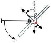
Figure 5: Fixed-wing UAV; the UAV antenna is indicated by a red dot. Front view of fixed-wing UAV performing a steady turn with a bank angle ${\varphi}_{e}$.

III-B1 Air-to-ground channels

The air-to-ground channel communication models the link between a UAV and a ground user, such as a control station or a 5G BS. The properties of this channel depend not only on the distance between both nodes, but also on the UAV altitude and on the elevation angle. As the elevation angle increases, the probability of LoS between both nodes also increases. As such, LoS links present lower losses than non-LoS links. As the UAV altitude increases, the elevation angle increases along with the distance between the nodes. For instance, one illustrative model that describes such effects is [104]:

$$\mathcal{H}(\mathbf{p}(t),\mathbf{q}(t))[dB] = -20\log\left(4\pi\lambda\|\mathbf{p}(t)-\mathbf{q}(t)\|_{2}\right)$$ (116)

$$+ \xi(\mathbf{p}(t),\mathbf{q}(t)),$$

where the first term represents the average path loss and $\xi(\mathbf{p}(t),\mathbf{q}(t))$ represents the shadowing. If there is line of sight, then $\xi(\mathbf{p}(t),\mathbf{q}(t))\sim\mathcal{N}(\mu_{LOS},\sigma_{\rm LOS}^{2})$. Otherwise, $\xi(\mathbf{p}(t),\mathbf{q}(t))\sim\mathcal{N}(\mu_{NLOS},\sigma_{NLOS}^{2})$. To complete this channel model, we must also consider the probability of having line of sight, which can be expressed as:

$$\mathrm{P}_{\rm LOS}(\mathbf{p},\mathbf{q})=\frac{1}{1+a\exp\left(-b\left[\frac{180}{\pi}\sin^{-1}\left(\frac{z_{UAV}}{\|\mathbf{p}-\mathbf{q}\|}\right)-a\right]\right)},$$ (117)

where $z_{UAV}$ is the altitude of the UAV, $\mathbf{p}_{UAV}$ is its position and $\mathbf{q}$ is the position of the ground node. The coefficients $a$ and $b$ are environment-dependent.

The model (116)-(117) does not take into account small-scale fading. As mentioned in [96], small-scale fading in air-to-ground channels often follows a Ricean distribution whose properties depend on the UAV altitude and the surroundings of the ground node. There are also approaches which use 3D numerical maps of the region of operation to determine the channel model [105]. We refer the reader to the survey in [96] for more detailed information about the air-to-ground UAV communications channels.

III-B2 Air-to-air channels

The modeling of ground-to-air channels is not yet well studied, but the situation for air-to-air channels (communications channels between flying UAVs) is worse still as there are fewer studies and measurement campaigns focusing on these types of channels [95]. When the altitude of two UAVs is low, the floor and other objects on the surface (e.g. hills, buildings, and trees) influence the channel. However, as the altitude of the UAVs increases, such influences weaken. As the altitude of both UAVs increases, the channel tends to consist of a LoS and tends to behave like the free-space channel described in section III-A1.

It has been observed experimentally that when the UAVs operate in an open field with a floor that is flat enough, the propagation channel follows a two-ray model [95]. As the altitude of the UAVs increases, the strength of the reflected path decreases. Further, when the UAVs are operating over bodies of water, such as lakes, the strength of the reflected path is stronger than when operating over land.

The constructive and destructive interference between the LoS and reflected waves described by the two-ray model can statistically be described with the small-scale fading. This is the approach taken in [106], where it was shown experimentally that the air-to-air channel model can be modelled as:

$$\mathcal{H}(\mathbf{p}(t),\mathbf{q}(t),t)=\frac{h(\mathbf{p}(t),\mathbf{q}(t),t)}{L_{P}(\mathbf{p}(t),\mathbf{q}(t))},$$ (118)

where the pathloss term $L_{P}(\mathbf{p}(t),\mathbf{q}(t))$ follows the free space model, and the small-scale fading term is well described by a Rician distribution with the height-dependent parameters:

$$p_{h}(x)=\frac{x}{\sigma_{0}^{2}}\exp\left(\frac{-x^{2}-\rho^{2}}{2\sigma_{0}^{2}}\right)I_{0}\left(\frac{x\rho}{2\sigma_{0}^{2}}\right),$$ (119)

where $x\geq 0$; $\rho$ and $\sigma$$=$$ah^{b}+c$ are the strength of the dominant and scattered components, respectively; $h$ is the altitude of the UAVs (both UAVs are assumed to have the same altitude); and with $a$, $b<0$, and $c$ being parameters to be fitted numerically according to the environment. Finally, we refer the reader to the survey in [95] for more detailed information about the air-to-air UAV communication channels.

III-C Performance metrics

In CaTP, the communication aspects are taken into consideration in the optimization problem in either the target function or the constraints. This requires the use of metrics to quantify the performance of wireless communication. Next, we discuss the metrics that are most relevant to CaTP.

Channel quality: one way in which the channel quality can be assessed is by measuring its power by using the Channel-to-noise Ratio (CNR) and the Signal-to-Noise Ratio (SNR). The instantaneous CNR [5] at the receiver is given by:

$$\mathrm{CNR}(\mathbf{p}(t),\mathbf{q}(t),t)={|\mathcal{H}(\mathbf{p}(t),\mathbf{q}(t),t)|^{2}}/{\sigma^{2}},$$ (120)

where $\mathbf{p}(t)$ and $\mathbf{q}(t)$ are the positions of the transmitter and the receiver, respectively, and $\sigma^{2}$ is the power of the thermal noise generated at the receiver. The mean CNR is $\mathbb{E}\left[\mathrm{CNR}(\mathbf{p}(t),\mathbf{q}(t),t)\right]$, where the expected value is taken w.r.t. small-scale fading and shadowing. The SNR is the CNR multiplied by the transmission power.

Another important metric is the Received Signal Strength (RSS) [107]. It measures the power of the received signal, with the reason behind its importance being that many receivers in the market provide the Received Signal Strength Index (RSSI) (a discretized version of the RSS). In practice, many algorithms resort to working with the RSSI.

Error rate: in some cases, one can be more interested in the performance of the communication system, rather than in the channel quality. The principal way of evaluating the performance of a communication system is by quantifying the errors that occurred in the transmission. This is done by calculating the Bit Error Rate (BER) or by the Packet Reception Ratio (PRR) [108], which measures how many packets were successfully received without errors. These metrics evaluate the performance of the communication system, and thus strongly depend on the specifications of the system, including the modulation scheme and the communication protocols.

Channel capacity: the channel capacity was first introduced by Claude Shannon in 1948 in [109]. It is an upper bound on the maximum bit rate, given channel conditions, for which an arbitrarily low BER can be reached. Its mathematical expression depends on the information that the transmitter and the receiver have about the channel, as well as on the power transmission strategy. When the channel is estimated at the receiver and the transmitter uses constant transmission power, then the channel capacity is given by [110]:

$$C=B\int_{0}^{\infty}\log_{2}\left(1+\gamma\right)p(\gamma)\mathrm{d}\gamma,$$ (121)

where $\gamma$ is the SNR, $p(\gamma)$ is its p.d.f., and $B$ is the bandwidth of the transmitted signal.

III-D Energy consumption

Although often the MR’s energy consumption is mostly due to motion, this is not always the case, as shown in the experiments presented in [51]. The $\mu$controller, the CPU, and the sensing systems can consume an amount of energy which may be comparable to the amount of energy spent in motion. The same applies to the MR’s communication system. The energy consumed by the communication system is mainly determined by the transmission power. Next, we discuss transmission strategies.

Constant power transmission: all signals are transmitted with constant average power. Thus, the transmitter’s energy consumption depends on the transmission time, but is independent of the transmitter and receiver positions. In this scenario, the SNR depends on the positions of the transmitter and the receiver through the spatial variations of the channel.

Adaptive power transmission: the transmitter adapts its power to ensure a certain power $P_{ref}$ for the received signal. The power is adapted as follows:

$$P={P_{\rm ref}}/{|\mathcal{H}(\mathbf{p}(t),\mathbf{q}(t),t)|^{2}}.$$ (122)

$P_{\rm ref}$ is selected to ensure a certain quality of service. The transmission power in (122) can take any arbitrarily large value. In practice, the transmission power is limited to a certain value $P_{max}$ by the hardware limitations, or by legal regulations. If the intended transmission power is smaller than $P_{max}$, then the actual transmission power is (122). Alternatively, if the intended transmission power is larger than $P_{max}$ (usually due to a poor channel gain), then it is not possible to satisfy the desired power $P_{ref}$ at the receiver. The most common action in this scenario is to refrain from transmitting and say that an outage has occurred. Thus, the transmission power can be written as:

$$P=\Bigg{\{}\begin{array}[]{cc}\frac{P_{\rm ref}}{|\mathcal{H}(\mathbf{p}(t),\mathbf{q}(t),t)|^{2}}&\mathrm{for}\ \frac{P_{\rm ref}}{|\mathcal{H}(\mathbf{p}(t),\mathbf{q}(t),t)|^{2}}\leq P_{\rm max},\\ 0&\mathrm{otherwise}.\end{array}$$ (123)

For mathematical simplicity and tractability, it is common to assume $P_{\rm max}\rightarrow\infty$ (i.e. disregard the power limitation).

Finally, the energy consumption at the receiver is generally considered constant. It is usually significantly lower than that of the transmitter, and is hence often neglected in the analysis.

III-E Final comments on communications models

We provided an overview of communication systems and basic channel models for both ground MRs and UAVs. We also discussed the special characteristics of UAV channel models. Another special scenario that can be important for some CaTP applications, such as rescue and search operations, regards communication inside tunnels and underground mines. These types of channel models are outside the scope of this tutorial, although interested readers are referred to [111, 71, 112].

The models presented in this section are narrowband models, which are the most basic models. More complex and elaborate models include wideband communication channel models, which take into consideration how the channel varies w.r.t. the frequency. Also, we must mention that when one of the transceivers moves quickly, Doppler shift occurs and affects the received signals. This phenomenon can be of particular importance when dealing with fixed-wing UAVs as they are capable of high speed flight.

IV Communications-aware Trajectory Planning

As mentioned in section I, CaTP refers to designing trajectories where both communications aspects (e.g. communication energy consumption, quality of the communications link, number of transmitted bits) and robotics aspects (e.g. kinematic and dynamic constraints, motion energy consumption) are simultaneously considered. We begin with some preliminary concepts. A particular case of CaTP is the Communications-aware Path Planning (CaPP) problem. The trajectory and path are defined as follows:

Definition 1 (Path).

The path followed by a robot from time instant $t_{1}$ to $t_{2}$ is defined as $\mathcal{P}(\mathbf{p}(t),t_{1},t_{2})\triangleq\{\mathbf{p}(t)|t\in[t_{1},t_{2}]\}$, where $\mathbf{p}(t)$ is the position of the robot at time $t$.

Definition 2 (Trajectory).

The trajectory followed by a robot from time instant $t_{1}$ to $t_{2}$ is the description of the robot’s position at each instant $t\in[t_{1},t_{2}]$ and can then be described as $\mathcal{T}(\mathbf{p}(t),t_{1},t_{2})=\{\mathbf{p}(t),t|t\in[t_{1},t_{2}]\}$.

The path consists of the collection of all the points visited by the MR without specifying when and without any velocity information. The trajectory gives not only information about the points visited by the MR, but also a temporal description of the change of the MR’s position over time. The trajectory can also be considered as the combination of the path and the velocity profile.

From the application point of view, a CaTP problem can be cast as either a CaR or a RaC task. We can also classify CaTP problems depending on what is being optimized into three categories. In the first category, the objective is to design the MR’s full trajectory, i.e., path and velocity profile; see for example [4]. In the second category, the translational velocity is given (e.g. constant speed) and the objective is to design the MR’s path; see for example [113]; this is a CaPP problem. In the third category, the path is given and the objective is to design the translational speed profile with which the MR will follow the given path; see for example [108].

CaTP problems can also be divided according to the trajectory type: predetermined and adaptive (also referred to as reactive). Predetermined trajectories are designed before they are executed by the MR, e.g. [4]. Adaptive trajectories are created and modified as the robot executes them, e.g. [98]; the MR may either use a predetermined trajectory as an initial guide and then implement an adaptive mechanism to adapt it in real-time in response to new information obtained from the environment, or create the trajectory in real-time while operating. Due to the elementary nature of this tutorial, we will mostly focus on predetermined trajectories, whose theory constitutes the base for adaptive ones.

The optimization method and the resulting optimal trajectory strongly depend on the available information about the wireless channel. The following are some possibilities.

i. Physical map available: in this case the Radio Frequency (RF) map or its estimate is known. In other words, we know $\mathcal{H}(\mathbf{p},\mathbf{q}(t),t)$ in Eq. (109) for all $\mathbf{p}\in\mathcal{W}$ and all $t\in[0,T]$ where $\mathcal{W}$ is the workspace where the MR operates and $\mathbf{q}(t)$ is the position of the other node.

For instance, in [114], the authors study the performance of different 3D path planners for a single UAV communicating over a cellular network. They resort to a realistic RF map to accurately evaluate the connectivity and the interference resulting from each path planning algorithm. This map is constructed as follows. First, a public 3D map of the region of Flanders, Belgium [115] is used. This map was generated by Lidar, with a latitude and longitude resolution of 1m$\times$1m, and each pixel contains the height of the surface. Then, using information from the Belgian Institute for Postal Services and Telecommunication, they located nineteen BSs of the Belgian mobile provider, Proximus, within the area of interest. The map was then fed into a 3D radio coverage simulator [116]. The latter uses both the 3D map and the location of the transceivers to determine whether or not a LoS exists, thus accounting for possible shadowing. To account for multipath fading, the simulator adds a Gaussian random process to the overall channel with a variance dependent on the altitude of the UAV. The resulting 3D RF map allowed the authors to observe how changes in altitude can improve communications performance.

If we have a physical 3D map of the workspace, then we can also obtain a 3D RF map by implementing ray tracing [73], [74], [75]. This type of RF map captures the shadowing (due to obstruction of the LoS), and can also capture multipath fading. 2D physical maps can also be used and can be useful particularly for ground MRs operating indoors to accurately determine when walls obstruct the LoS.

ii. RF channel measurements available: in this case, we do not have a physical map of the workspace where the MRs operates, but we have a number of RF channel measurements taken at different locations in the workspace. Thus, prior to solving the CaTP, we feed the channel measurements into a predictor to create an RF map that will be used by the trajectory planner. In [117], the authors consider a ground MR that must visit a number of points of interest, gather data there, and then transmit all collected data to a BS. This must be done while minimizing the total energy consumed. The MR initially disposes of few channel measurements taken in the workspace. These measurements are then fed into the probabilistic channel assessment framework developed by the authors in [78] and [79]. This framework is used by the path planning algorithm to predict the channel gain throughout the workspace. The predicted probabilistic RF map is constructed using the pathloss model, the Probability Density Function (p.d.f.) of the multipath fading, and the p.d.f. of the shadowing as well as its spatial correlation.

iii. Mathematical model available: in this case, we only dispose of a mathematical model of the communications channel. In our previous work [4], we considered the problem of a multirotor UAV that must reach some goal while transmitting data to a BS. The only information about the communications channel used for solving the communications-aware trajectory planning was the pathloss model and the p.d.f. of the shadowing. In [118], the authors considered the problem of optimizing the position of a UAV operating as a BS. To solve this, they considered the pathloss model, which is complemented by the Probability Mass Function (p.m.f.) of the LoS. In [119], we considered the problem of mitigating the small-scale fading in an MR communications link by leveraging the knowledge of its p.d.f. and spatial correlation. ∎

IV-A General Structure

The CaTP optimization problem to determine a predetermined trajectory of a single MR can be formulated as:

$$\begin{array}[]{l}\displaystyle\operatorname*{minimize}_{\mathcal{C},\mathcal{T}}\ J(\mathcal{C},\mathcal{T})\\ {\rm s.t.}\\ {\rm motion\ model},\\ {\rm channel\ model},\\ {\rm trajectory\ constraints},\\ {\rm communications\ constraints},\end{array}$$ (124)

where $\mathcal{C}$ is the set of all communication-related parameters to be optimized, such as modulation order or transmission power; and $\mathcal{T}$ is the set of variables related to the trajectory of the robot, such as the completion duration of the trajectory or the waypoints that form the robot’s path.

For instance, in [28], $\mathcal{T}$ consists of the set of UAV’s 3D hovering locations as well as their visiting order, and communications-related inputs were considered, i.e., $\mathcal{C}=\emptyset$. In [117], $\mathcal{T}$ consists of the set of waypoints forming the robot’s path, and $\mathcal{C}$ describes the spectral efficiency (i.e. the bit rate normalized by the bandwidth) of the robot’s transmitter. In [118], $\mathcal{T}$ describes the 3D position of the UAV, and $\mathcal{C}$ is the set of users that the UAV communicates with. In [14], the inputs forming $\mathcal{T}$ are the position, velocity, and acceleration profiles of the UAV, and those forming $\mathcal{C}$ are the transmission powers of the UAV and the BS. In [4], $\mathcal{T}$ consists of the control signals for the UAV motors, and $\mathcal{C}=\emptyset$. In [120], $\mathcal{T}$ consists of the altitude of the UAV, and $\mathcal{C}$ consists of the beamwidth of its antennas.

The generic CaTP problem in (124) is composed of five elements: the optimization target $J(\mathcal{C},\mathcal{T})$, a motion model for the MR describing how its state behaves according to the control signal $\mathbf{u}$ (discussed in Section II), a wireless channel model describing how the received and transmitted signals behave depending on the position and orientation of the MR (discussed in section III), some trajectory related constraints, and constraints related to the communication system performance and/or goals. We will next discuss the elements of the CaTP problem that have not been discussed in previous sections.

IV-B Optimization target

By convention, optimization problems are usually stated as minimization problems [121], as in (124). However, sometimes (e.g. when the focus is on energy efficiency or on maximizing the number of users served), they are initially cast as maximization problems [14], [12], [118]. Nevertheless, any maximization problem can be converted into an equivalent minimization problem by proceeding as follows [121]:

$$\begin{array}[]{ccc}\displaystyle\operatorname*{maximize}_{\mathcal{C},\mathcal{T}}\ J(\mathcal{C},\mathcal{T})&\rightarrow&\displaystyle\operatorname*{minimize}_{\mathcal{C},\mathcal{T}}\ -J(\mathcal{C},\mathcal{T}).\end{array}$$ (125)

Another possibility is the following transformation:

$$\begin{array}[]{ccc}\displaystyle\operatorname*{maximize}_{\mathcal{C},\mathcal{T}}\ J(\mathcal{C},\mathcal{T})&\rightarrow&\displaystyle\operatorname*{minimize}_{\mathcal{C},\mathcal{T}}\ J^{-1}(\mathcal{C},\mathcal{T}).\end{array}$$ (126)

The linear transformation in (125) maintains the properties of the original optimization target regardless of its nature. The nonlinear transformation (126) deforms the original optimization target by expanding it for values in the region $[-1,1]$ and compressing it outside of this interval. Furthermore, if the original optimization target $J(\mathcal{C},\mathcal{T})$ can take a value of zero, then $J^{-1}(\mathcal{C},\mathcal{T})$ will not be defined at this value. Nevertheless, if $J(\mathcal{C},\mathcal{T})>0$ (or $J(\mathcal{C},\mathcal{T})<0$), then the nonlinear transformation (126) is not necessarily an issue. For instance, the authors in [120] transform a minimization problem into a maximization problem by applying the nonlinear transformation (126) to a strictly positive optimization target. The authors in [122] move in the opposite direction of the nonlinear transformation (126); instead of minimizing the power consumption, they maximize the inverse of the power consumption to simplify the problem.

If the inputs of the optimization problem (i.e. $\mathcal{C}$ and $\mathcal{T}$) are variables, then the optimization target is a function, e.g. [123, 7]. On the other hand, if the inputs of the optimization problem are functions, then the optimization target is a functional [124], e.g. [119, 21, 125]. Further, if the optimization target is a function to be minimized, it is referred to cost function. Alternatively, if the optimization target is a function to be maximized, it is referred to as utility function [121]. Similarly, if the optimization target is a functional to be minimized, it is referred to a cost functional [5, 8].

If the set of inputs $\{\mathcal{C},\mathcal{T}\}$ contains continuous variables/functions and discrete variables/functions, the optimization problem is referred to as mixed-integer. A common class of mixed-integer optimization problems which often appears in CaPP is the Mixed-Integer Linear Programming (MILP) [117, 126, 127, 128].

We next describe some functionals that have been used as optimization targets. We start with the optimization target initially considered in [4] which aims to solve a CaTP problem for a multirotor UAV :

$$J=\vartheta\int_{0}^{t_{f}}\|\mathbf{u}(t)\|_{2}^{2}\mathrm{d}t+(1-\vartheta)w(\mathbf{p}),$$ (127)

where $t_{f}$ is the trajectory duration and $w(\mathbf{p})$ is an arbitrary functional related to a communications criteria which depends on the trajectory of the UAV. The optimization target consists of the sum of two terms, the first one measuring the motion-induced energy consumption, while the second one is a communications-related term which depends on the bit rate over the UAV trajectory. Parameter $\vartheta\in[0,1]$ determines the importance of one term over the other. The control signal for the UAV is $\mathbf{u}(t)\in\mathbb{R}^{4}$, defined in $t\in[0,t_{f}]$ (i.e. $\mathbf{u}$ is a four dimensional vectorial function defined over a closed support). The 3D position of the UAV is $\mathbf{p}(t)\in\mathbb{R}^{3}$, defined in $t\in[0,t_{f}]$ (i.e. $\mathbf{p}$ is a three dimensional vectorial function defined over a closed support). The model in [4] used to describe the relationship between the UAV control signal $\mathbf{u}$ and its position $\mathbf{p}$ is as described in subsection II-B. Therefore, the optimization target $J$ depends on two functions: the UAV control signal $\mathbf{u}$ and the UAV position $\mathbf{p}$ (which itself depends on $\mathbf{u}$). Furthermore, the optimization target is the convex combination of two functionals.

Another interesting example can be found in [125]. In this case, a MR disposes of a fixed time $T$ to harvest radio energy from a BS. The channel experiences small-scale fading, and the radio energy harvested varies greatly over very small distances. Thus, the MR uses the following procedure divided in three phases: during the first phase, the MR moves along a line of length $L$ for a duration of $\alpha T_{s}$ with $\alpha\in(0,1)$ and $T_{s}<T$; during the second phase, the MR moves to the position in the line with the highest channel gain; lastly, the MR remains for the rest of the time (i.e. $T-T_{s}$) at that position harvesting radio energy. The objective is to optimize the velocity profile of the MR to maximize the expected value of the harvested energy. Therefore, the optimization target is:

$$J = E_{s}(v^{I}_{{}_{L,\alpha,T_{s}}})+E_{s}(v^{II}_{{}_{L,\alpha,T_{s}}})+E_{H}(L,T_{s})$$ (128)

$$- E_{m}(v^{I}_{{}_{L,\alpha,T_{s}}})-E_{m}(v^{II}_{{}_{L,\alpha,T_{s}}}),$$

where $v^{I}_{{}_{L,\alpha,T_{s}}}$ and $v^{II}_{{}_{L,\alpha,T_{s}}}$ are the speed profiles of the MR in the first and second phases, respectively. They are both unidimensional continuous functions parametrized by the variables $L$, $\alpha$, and $T_{s}$. The support for $v^{I}_{{}_{L,\alpha,T_{s}}}$ is $t\in[0,\alpha T_{s}]$ and the support for $v^{II}_{{}_{L,\alpha,T_{s}}}$ is $t\in[\alpha T_{s},T_{s}]$. The first term in (128) is the energy harvested during the first phase while using the speed profile $v^{I}_{{}_{L,\alpha,T_{s}}}$; the second term is the energy harvested during the first phase while using the speed profile $v^{II}_{{}_{L,\alpha,T_{s}}}$; the third term is the energy harvested at the optimum position found by the MR. This energy depends on the length $L$ (the space where the MR searched for the position with the largest channel gain) and the time spent harvesting energy at the position with the largest channel gain; the fourth term is the energy spent by the MR in motion during the first phase; the fifth term is the energy spent by the MR in motion during the second phase. From the above description, we can observe that the optimization target (128) is the sum of four functionals ($E_{s}(v^{I}_{{}_{L,\alpha,T_{s}}})$, $E_{s}(v^{II}_{{}_{L,\alpha,T_{s}}})$, $E_{m}(v^{I}_{{}_{L,\alpha,T_{s}}})$, and $E_{m}(v^{II}_{{}_{L,\alpha,T_{s}}})$) and one function $E_{H}(L,T_{s})$ (which depends on the variables $L$ and $T_{s}$). In this problem, the functions $v^{I}_{{}_{L,\alpha,T_{s}}}$ and $v^{II}_{{}_{L,\alpha,T_{s}}}$ are actually parameterized by the variables $L$, $\alpha$, and $T_{s}$. Nevertheless, in [125], we use calculus of variations [129] to find the optimum shape of the speed profiles (i.e. the functions $v^{I}_{{}_{L,\alpha,T_{s}}}$ and $v^{II}_{{}_{L,\alpha,T_{s}}}$) parameterized with $L$, $\alpha$, and $T_{s}$. After this step, the functionals in (128) become functions of $L$, $\alpha$, and $T_{s}$.

The general strategy for converting functionals into functions is to fix the shape of the function that constitutes the input to the functional. One way to do this is to derive the optimum shape, as described in the previous example. However, this is not always possible, at least not analytically, due to the complexity of the problem. An alternative is to use the method presented in [7]. In the latter, we considered a UAV acting as a data ferry between a source and a destination. The objective was to optimize the UAV’s periodic trajectory, of period $T$, to maximize an upper bound of the number of bits transferred. During the first half of the trajectory, the UAV collects data from the source and delivers it to the destination in the second half. The corresponding functional to maximize is:

$$J=\int_{0}^{T/2}r({x}(t),{y}(t))\mathrm{d}t,$$ (129)

where functions $x(t)$ and $y(t)$ represent the trajectory of the UAV at time instant $t$ in the $x-y$ plane, and the integrand in (129) is the maximum instantaneous bit rate achievable at $(x,y)$. The integral represents the maximum amount of bits collected by the UAV from the source. The functional (129) depends on the unidimensional continuous functions $x(t)$ and $y(t)$, with support $t\in[0,T]$. Since the problem indicates that the optimum UAV trajectory is periodic, one way to transform the functional (129) into a function is by constraining the shape of the functions $x(t)$ and $y(t)$ using a Fourier series of order $N$. After adding this constraint into the optimization problem, the functional (129) becomes a function of the Fourier series coefficients. The resulting optimum trajectory is suboptimal. It gets closer to the optimum trajectory as the order of the Fourier series grows, but this also increases the number of parameters to optimize.

Below we briefly review some of the communications-related and robotics-related terms used in the optimization target of CaTP problems. In [130], the communications-related term is the outage probability of the communication link. In [118], the optimization target is the number of users served by a UAV operating as an aerial BS. In [131], the communications-related term is the coverage radius of a Low-altitude aerial platform (LAP) acting as a BS for ground users. In [120], the communications-related terms are the time that the UAV takes to transmit a certain amount of data, and the total amount of bits transmitted by the UAV. In [119], the optimization target includes the expected value of the channel gain. In [117], the communications-related term considered in the optimization target is the energy spent in data transmission.

In [28], the authors consider a multirotor UAV and a cost function which has two robotics-related terms: the time that the UAV takes to complete the trajectory and the time that it spends hovering over ground nodes. In [117], the authors consider an MR moving at constant speed, and a cost function which consists of the motion-induced energy consumption in the form of (34). In [14], the authors aim to maximize the efficiency of a fixed-wing UAV acting as a communications relay; the cost function represents the propulsion-induced energy consumption in the form of (108).

IV-C Trajectory constraints

These constraints directly restrain the shape of the trajectory and the time in which it is completed.

One simple constraint in this category defines the area where the MR can operate. For example, the authors in [86] constrain the area where the MR can move by $\mathbf{p}(t)\in\mathcal{W}/\mathcal{Q}_{t}$, where $\mathbf{p}(t)\in\mathbb{R}^{2}$, $\mathcal{W}\subset\mathbb{R}^{2}$ is the workspace and $\mathcal{Q}_{t}$ is the set of points where channel measurements have been taken up to the instant $t$. In [126], the authors define the environment $\mathcal{X}$ as a large convex polygonal subset of the 2-D Euclidean space $\mathbb{R}^{2}$, define $\mathcal{X}_{obs}\subseteq\mathcal{X}$ as the regions in the environment occupied by polygon obstacles.

The shape of the trajectory can be constrained to polynomials [132] or splines [133]. One reason for using such constraints is that the resulting optimum trajectory can be feasible for real-life robots [98]. Various types of polynomials can be used, each with its own particular properties (e.g. Chebyishev polynomials [134], Laguerre polynomials [135]). More information about the relationship between this type of constraint and the trajectory’s feasibility and smoothness can be found in [136] and the references therein.

We can also constrain the initial and/or final positions of the robots [108], [12] by adding the trivial constraints:

$$\mathbf{p}(0)=\mathbf{p}_{\rm ini}, \mathbf{p}(t_{f})=\mathbf{p}_{\rm fin}.$$ (130)

If the initial and final positions differ (see [12, 137]), we have an open trajectory. If they are the same ([138, 7]), we have a closed trajectory. We find closed trajectories in repetitive tasks, such as a multirotor UAV operating as a data ferry [7], an MR doing periodic data collection from sensor nodes [128], or a fixed-wing UAV acting as a communications relay [138, 31]. Further, a predetermined trajectory that is periodic and smooth can be well approximated by truncated Fourier series.

Another type of constraint aims at limiting the velocity and/or acceleration of the robot. In [139], the authors consider a group of $N$ MRs and limit the speed of each one using the following constraint:

$$\|\dot{\mathbf{p}}_{n}\|_{\infty}\leq V_{n},$$ (131)

where $\dot{\mathbf{p}}_{n}\in\mathbb{R}^{2}$ is the velocity of the $n$th MR, and $V_{n}$ is a design parameter. The authors mention that they used the $H_{\infty}$-norm to limit the MRs speed instead of the $\ell_{2}$-norm in order to keep their particular optimization problem as a linear program. Nevertheless, the use of the $\ell_{2}$-norm to directly limit the speed is very common [137, 11]. In the case of multirotor UAVs, it is also common to separately limit the horizontal speed and the vertical speed [140], [141]. Sometimes, constraints limit not only the speed, but also the acceleration of the MR [29]. One may also set lower and upper bounds on the velocities and accelerations [142].

The previous constraints directly limit the velocity of the UAV, but other constraints indirectly perform this by acting on the inputs to the dynamic model of the UAV. For instance, the authors in [143] limit the rotational speed and acceleration of the rotors.

IV-D Communications constraints

These constraints act on the overall communication system performance or directly on the wireless channel experienced by the MR along the whole trajectory. When stochastic channel models are used, the constraints related to the wireless channel are probabilistic. For example, the authors in [28] consider the problem of a multirotor UAV in a dense Internet of Things (IoT) network that visits $M$ hovering locations where it collects data from the connected nodes. The ground-to-air channels experience Nakagami-$m$ fading. Depending on the Signal-to-Interference-and-Noise Ratio (SINR) which itself depends on the hovering locations, the probability of successfully collecting data from the covered sensors can vary. Therefore, the authors add the following probabilistic constraint to their problem:

$$\sum_{\ell=1}^{M}\mathbb{E}[K_{\ell}]\geq N,$$ (132)

where $K_{\ell}$ is the number of successfully collected observations at the $\ell$th hovering location, and $N$ is the minimum desired average number of successful observations that the UAV must collect from the IoT network. In [117], the authors consider the problem of an MR that must visit $m$ Points of Interest (POI), gather their data, and then transmit it to a BS. The MR can transmit with $n_{r}$ different spectral efficiencies. The MR can choose to transmit data from the current POI or from other $n_{s}$ communication points close by to compensate for small-scale fading. The authors include the following constraint:

$$\sum_{2}^{m}\sum_{j=1}^{n_{s}+1}\sum_{k=1}^{n_{r}}R_{k}t_{i,j,k}=V/B,$$ (133)

where $R_{k}$ is the $k$th spectral efficiency, $V$ is the total number of bits collected from the POIs, $B$ is the bandwidth used in the transmission, and $t_{i,j,k}$ is the time spent by the MR transmitting at the $j$th communication point of the $i$th POI using the spectral efficiency $R_{k}$. Note that even if both [28] and [117] consider a stochastic channel model, the constraint (132) is stochastic but the constraint (133) is deterministic. This is due to the fact that the constraint (132) acts on the received bits, which is a stochastic process (due to the stochastic channel model), whereas the constraint (133) acts on the transmitted bits, which is a deterministic process. In [29], the authors consider a multirotor UAV acting as a BS and providing communications to ground users. The transmitter of the UAV has a bandwidth $B$ divided into $N_{F}$ orthogonal subcarriers. The authors include the following constraint to ensure that each user is provided with at least a specified minimum bit rate:

$$\sum_{i}^{N_{F}}\left(\frac{s_{k}^{i}[n]B}{N_{F}}\right)\log_{2}\left(1+\gamma_{k}^{i}[n]\right)\geq R_{k}^{req},\,\,\forall k,n$$ (134)

where $s_{k}^{i}[n]=1$ if the $k$th user is assigned the $i$th subcarrier by the UAV at time $n$, and $s_{k}^{i}[n]=0$ otherwise, $B/N_{F}$ is the bandwidth of each subcarrier, $\gamma_{k}^{i}[n]$ is the SNR, of the channel between the $k$th user and the UAV on the $i$th subcarrier at instant $n$, and $R_{k}^{req}$ is the minimum bit rate required by the $k$th user. The constraint (134) ensures that, at all times, the achievable data rate of each user is at least $R_{k}^{req}$. In [29], the optimization problem was formulated in discrete time. We can find similar constraints in [144] where a UAV serves $K$ users and a minimum bit rate for each one must be ensured. Similarly, in [145], a UAV acts as a communications relay between a ground user and a BS and a constraint is added to ensure a minimum bit rate on each communications link.

We can also constrain the average number of bits that the robot must transmit to have a lower bound:

$$\int_{0}^{T}\mathbb{E}[R({\rm SNR}(\mathbf{p}(t),\mathbf{q}(t),t))]\mathrm{d}t\geq N,$$ (135)

where ${\rm SNR}(\mathbf{p}(t),\mathbf{q}(t),t)$ is the instantaneous SNR at time $t$ over the link between the MR located at $\mathbf{p}(t)$ and the other node located at $\mathbf{q}(t)$. The function $R(\cdot)$ determines the transmission bit rate as a function of the instantaneous SNR. This function $R(\cdot)$ depends on the modulation scheme as well as on the bandwidth of the transmitted signal. The expected value in (135) is taken w.r.t. the joint p.d.f. of the shadowing and small-scale fading. To introduce this constraint, the designer needs to know the first-order statistics of the wireless channel model. Because of the stochastic nature of the wireless channel, the constraint (135) does not ensure that the MR will be able to always transmit at least $N$ bits, but rather that following the same trajectory in the same environment it will transmit at least $N$ bits on average. Note that (135) assumes that the transmission process is continuous (the integrand in (135) is treated as a continuous function of time). Even if the transmission is not continuous (e.g. when data is transmitted in packets and not in a continuous and uninterrupted flow), we can assume in practice that it is a continuous process since the dynamics of the motion is generally much slower than those of data transmission.

When formulating the problem in discrete time and dealing with Decode-and-Forward (DF) relays, there is a common constraint called Information Causality Constraint (ICC) [146, 13, 14, 147]: at time slot $n$, the DF relay receives data from a source, processes it, and then transmits it at the next time slot to the destination. For instance, in [146], the ICC is included in the discrete-time optimization problem as follows:

$$\sum_{i=2}^{n}\log_{2}\left(1+p_{r}[i]\gamma_{rd}[i]\right)\leq\sum_{i=1}^{n-1}\log_{2}\left(1+p_{s}[i]\gamma_{sr}[i]\right),$$ (136)

where $\gamma_{sr}[i]$ and $\gamma_{rd}[i]$ are the CNR at discrete time slot $i$ of the source-to-relay and relay-to-destination links, respectively, and $p_{s}[i]$ and $p_{r}[i]$ are the transmission powers at discrete time slot $i$ of the source and of the relay, respectively. The argument of the left term represents the achievable bit rate in the relay-to-destination link at slot $i$, while the argument of the right term represents the achievable bit rate in the source-to-relay at slot $i$. The ICC (136) ensures that at time slot $n$, the relay cannot transmit to the destination more bits than the maximum number of bits it had already processed from the source, hence the term causality. We must mention that the Amplify-and-Forward (AF) relays operate differently from the DF relays, and thus the ICC should be adapted accordingly.

There are also constraints acting directly on the wireless channel; the advantage of such constraints resides in the fact that it makes the optimisation problem independent of the used communication system (e.g. modulation type, AF or DF relay). For instance, when the channel model is stochastic, we cannot ensure that the CNR will take a certain value $\gamma_{0}$, but we can add a constraint to ensure that it achieves this value $\gamma_{0}$ with a desired probability $\eta$:

$$\mathrm{Pr}\left({\rm CNR}(\mathbf{p}(t),\mathbf{q}(t),t)\geq\gamma_{0}\right)=\eta,\ \forall\ t\in[0,T],$$ (137)

where $\mathbf{p}(t)$ and $\mathbf{q}(t)$ are the positions of the transmitter and receiver at time $t$, and $T$ is the duration over which the constraint must be enforced. We find a similar constraint in [122, 148] where the authors use expected values rather than probabilities to deal with the stochasticity of the communications channels. In [149], the authors introduce a constraint limiting the maximum path loss allowed, which acts only on the deterministic part of the wireless channel.

Another class of constraints act on the communications coverage. They can act either in space [150, 118] or in time [151]. The authors in [118] consider a UAV acting as an aerial BS for a group of ground users $\mathcal{U}$ and aim to maximize the number of users served. To solve this problem, the authors use the following constraint:

$$R(h)\geq r_{i}-M(u_{i}-1),\,\,\forall\,\,i=1,\cdots,|\mathcal{U}|,$$ (138)

where $R(h)$ is the communications coverage radius of the UAV, which depends on its altitude $h$, $r_{i}$ is the horizontal distance between the $i$th user and the BS, $\{u_{i}\}_{i=1}^{|\mathcal{U}|}$ are binary allocation variables to be optimized (if $u_{i}=1$, then the $i$th user is served by the UAV and $u_{i}=0$ otherwise), and $M>\displaystyle\max_{i}\{r_{i}\}$ is a design parameter. The constraint (138) works as follows. If we allocate the $i$th user to the aerial BS (i.e. $u_{i}=1$), then (138) is satisfied only if that user is within the coverage area. On the other hand, if we do not allocate the $i$th user to the aerial BS (i.e. $u_{i}=0$), then the constraint (138) becomes satisfied regardless of its horizontal distance $r_{i}$ to the aerial BS. In [151], the authors consider a UAV navigating in an area sparsely covered by ground BSs. The objective is to reach a final destination in minimum time $T$, but to ensure that the UAV does not spend more than $\tau_{\rm max}$ continuous seconds outside the coverage area the following constraint is used:

$$\rho(t)-t-1\leq\tau_{\max},$$ (139)

where $\rho(t)=\operatorname*{argmin}_{\forall s>t}\{c_{s}=1\}$ with:

$$c_{t}=\Bigg{\{}\begin{array}[]{cc}1&\mathrm{if}\,\exists\,\mathbf{g}_{k}\in\mathcal{G}\,:\|\mathbf{g}_{k}-\mathbf{p}(t)\|\leq R,\\ 0&\mathrm{otherwise},\end{array}$$ (140)

where $\mathcal{G}$ is set containing the positions of all the BSs, $\mathbf{g}_{k}$ is the position of the $k$th BS, and $R$ is the coverage range of the BSs.

Other constraints act on the transmission power. For example, the authors in [137] consider a UAV equipped with a transmitter that has power control capacity and constrain the average transmission power:

$$\frac{1}{N}\sum_{n=1}^{N}p[n]\leq P,$$ (141)

where $p[n]$ is the power transmitted by the UAV at discrete time $n$, $N$ is the duration of the UAV trajectory, and $P$ is the maximum average power allowed. In [29], the authors consider a UAV with a transmitter with $N_{F}$ subcarriers to serve $K$ users. The authors constrain the maximum instantaneous transmission power as:

$$\sum_{i=1}^{N_{F}}\sum_{k=1}^{K}s_{k}^{i}[n]p_{k}^{i}[n]\leq P_{\max},$$ (142)

where $s_{k}^{i}[n]$ is a binary allocation variable. If at time $n$, the $i$th subcarrier is allocated to the $k$th user, then $s_{k}^{i}[n]=1$; otherwise, $s_{k}^{i}[n]=0$. The power transmitted by the UAV to the $k$th user through the $i$th subcarrier is $p_{k}^{i}[n]$. The overall sum in the left term of (142) is the total power transmitted by the UAV at time $n$. Both constraints (141) and (142) make sense for diverse reasons, among them we find the properties of the power amplifier of the RF transmitter. Indeed, the RF amplifier is a nonlinear device. Hence, while it is possible that the average power of the signal transmitted operates within the linear region of the amplifier, if the maximum instantaneous power is unconstrained, then the peak power may drive the RF amplifier to operate in the nonlinear region and thus lead to distortion. This will degrade the performance of the communication [152, 153].

The energy consumed in communications can sometimes be comparable to the energy spent in motion. This is reflected in [29], where the authors consider a UAV equipped with solar panels for energy harvesting and providing communication to ground users. To ensure the continuous operation of the UAV, the authors add the following constraint:

$$\left(\frac{1}{\epsilon}P_{\rm tx}[n]+P_{\rm UAV}[n]+P_{\rm static}\right)\Delta_{T}\leq q[n],\,\forall n,$$ (143)

where $P_{\rm tx}[n]$ is the power transmitted at discrete time $n$, $P_{\rm UAV}[n]$ is the aerodynamic power consumption of the UAV, $P_{\rm static}$ is the static power required to maintain the operation of the UAV, $\Delta_{T}$ is the sampling duration of the UAV controller, and $q[n]$ is the energy level of the battery. The energy harvested from the sun does not appear in (143) because in this system the solar panels are only connected to the battery, so they cannot directly power the other systems of the UAV. ∎

IV-E Soft Constraints

The constraints discussed above are hard constraints, i.e., either they are satisfied or they are not. In some cases, hard constraints can cause feasibility issues in the optimization problem [154]. It might be that some combination of parameter values makes it impossible to satisfy every single hard constraint in the optimization problem, rendering it unfeasible. In complex CaTP problems it might be hard to identify this situation. This can be addressed by relaxing some hard constraints and transforming them into soft constraints [155, 156, 157]. The idea of soft constraints is to allow violations but impose a penalty depending on the extent of the violation.

In CaTP, some constraints are imposed by the physical world. For example, the energy constraint (143) states that the UAV cannot consume more energy than the energy stored within its battery, as this constraint is imposed by the laws of physics and cannot be relaxed. On the other hand, other constraints are arbitrarily imposed by the designer. For example, for the constraint in (130), the final position of the robot is arbitrarily imposed by the designer. Thus, if the robot finishes its trajectory at $\mathbf{p}_{fin}+\bm{\epsilon}$ with a small $\|\bm{\epsilon}\|_{2}$, rather than at exactly $\mathbf{p}_{fin}$, there would probably not be a problem. Similarly, in the constraint (134), the minimum achievable bit rate $R^{req}_{k}$ is arbitrarily imposed by the designer. If a user experiences a bit rate slightly inferior to the desired minimum bit rate, it might pass unnoticed. These constraints are the ones that can be relaxed and converted into soft constraints.

There are various methods to implement soft constraints, but we will discuss only three of them. The first method consists of the use of slack variables [156, 154, 121]. We can use them to relax inequality constraints. For instance, consider the following generic optimization problem with hard constraints:

$$\operatorname*{minimize}_{x} J(x)$$

$$\mathrm{s.t.}$$ (144)

$$g(x)\leq 0,\quad f(x)=c,$$

where $x,J(x),g(x),f(x),c$$\in$$\mathbb{R}$. We can relax the hard inequality constraint imposed on $g(x)$ with a slack variable $s$:

$$\operatorname*{minimize}_{x,s} J(x)+k_{1}s^{2}$$

$$\mathrm{s.t.}$$ (145)

$$g(x)\leq s,\quad s\geq 0,\quad f(x)=c,$$

where $k_{1}>0$ is a design parameter. In (IV-E), we can have $g(x)>0$ since the slack variable $s$ will take the necessary value to satisfy the constraint $g(x)\leq s$. Nevertheless, this adds a penalty $k_{1}s^{2}$ to the cost function. If $g(x)\leq 0$, then $s=0$. The relaxed optimization problem needs to optimize not only the variable $x$ but also $s$. In [12], we find an interesting example where a CaTP has its cost function exclusively composed of a single slack variable.

The second method consists of the use of exponential penalty functions [158] to relax the inequality functions:

$$\operatorname*{minimize}_{x} J(x)+\frac{k_{1}}{k_{2}}\left(\exp{\left(k_{2}\,g(x)\right)}-1\right)$$

$$\mathrm{s.t.}$$ (146)

$$f(x)=c,$$

where $k_{1},k_{2}>0$. If $g(x)=0$, the penalization term becomes exactly zero. If $g(x)<0$ and $k_{2}\rightarrow+\infty$, then the penalization term tends to zero and its effect vanishes. If $g(x)>0$, then the penalization term becomes larger. In [4], we used exponential penalization to avoid obstacles in a CaTP problem.

The third method is to transfer the equality constraints to the optimization target as quadratic penalizations [157, 155]:

$$\operatorname*{minimize}_{x} J(x)+k_{1}|f(x)-c|^{2}$$

$$\mathrm{s.t.}$$ (147)

$$g(x)\leq 0,$$

where $k_{1}>0$. The penalization term in (IV-E) is small if $f(x)$ is close to the desired value $c$, and the farther $f(x)$ from $c$, the larger the penalization. In [159], the authors consider a CaTP with multiple MRs and they add to their cost functional the same type of penalization as in (IV-E).

We can simultaneously relax the inequality and equality constraints by combining the use of slack variables and the quadratic penalization terms:

$$\operatorname*{minimize}_{x,s} J(x)+k_{1}|f(x)-c|^{2}+k_{2}s^{2}$$

$$\mathrm{s.t.}$$ (148)

$$g(x)\leq s,\quad s\geq 0,$$

If the original problem (IV-E) is feasible, then all of its hard constraints are satisfied by the optimum solution $x^{*}$. Consequently, the relaxed problems (IV-E), (IV-E), and (IV-E) are equivalent to (IV-E), and (IV-E) will tend to be equivalent to (IV-E) as $k_{2}\rightarrow+\infty$. Alternatively, if the original problem (IV-E) is unfeasible, the relaxed problem (IV-E) is still feasible; by tuning $k_{1}$ and $k_{2}$, we can get as close as possible to satisfying the original hard constraints.

V CaTP Examples

Next, we first describe in detail three illustrative examples of CaTP problems that were carefully selected to showcase the variety of mathematical forms that CaTP problems can take. Then, we present a survey of minimum energy CaTP problems, a survey of energy efficient CaTP problems, and finally a survey of the different types of CaTP problems.

Example 1. An MR is tasked to move in a finite time $t_{f}$ from an initial position $\mathbf{p}_{ini}$ to a final position $\mathbf{p}_{fin}$ while transmitting a given number of bits $c$ to a BS with a certain bit error probability. The objective is to optimize the trajectory and the instantaneous bit rate to balance the motion energy and the energy spent in transmission.

The input to the MR is the control signal $\mathbf{u}(t)\in\mathbb{R}^{2}$, which directly controls its acceleration. The communications input is the instantaneous transmission bit rate $R(t)\in\mathbb{R}$. Note that $\mathbf{u}(t)$ and $R(t)$ are both functions with support $[0,t_{f}]$.

In this example, the state vector of the system is $\mathbf{x}^{\mathrm{T}}=[\mathbf{x}_{1}^{\mathrm{T}}(t)\,\,\mathbf{x}_{2}^{\mathrm{T}}(t)\,\,{x}_{3}(t)]$, where $\mathbf{x}_{1}(t)\in\mathbb{R}^{2}$ and $\mathbf{x}_{2}(t)\in\mathbb{R}^{2}$ are the MR position and velocity, and ${x}_{3}(t)\in\mathbb{R}$ is the number of bits transmitted by the MR.

The optimization problem is cast as a maximization problem with the following cost functional:

$$J(\mathbf{x},\mathbf{u},R) = \int_{0}^{t_{f}}\left(\frac{(2^{R(t)}-1)s(\mathbf{x}_{1}(t))}{K}\right)\mathrm{d}t$$ (149)

$$+ \gamma\int_{0}^{t_{f}}p_{2}\left(\|\mathbf{x}_{2}(t)\|_{2},\|\mathbf{u}(t)\|_{2}\right)\mathrm{d}t$$

$$+ C_{1}\|\mathbf{x}_{1}(t_{f})-\mathbf{p}_{\rm fin}\|^{2}+C_{2}\|\mathbf{x}_{2}(t_{f})\|^{2}$$

$$+ C_{3}\|{x}_{3}(t_{f})-c\|^{2}.$$

The first term in the functional corresponds to the energy spent in transmission, where the transmitter of the MR has a power control mechanism that sets $K=-1.5/\log(5p_{b})$ to adapt the transmission power to ensure a BER $p_{b}$. The integrand of this first term corresponds to the power required to meet the targeted BER with the transmission bit rate $R(t)$, as well as the CNR estimation $s(\mathbf{x}_{1}(t))$ at position $\mathbf{x}_{1}(t)$. The second term is the motion-induced energy, weighted by parameter $\gamma>0$, with $p_{2}(a,b)$ being a second-order polynomial in $a$ and $b$; the integrand is the instantaneous power consumed in motion. The last terms are quadratic penalties on the desired final states of the system. $C_{1},C_{2},C_{3}>0$ are design parameters that determine the importance of reaching the desired final states. The first penalty moves the final MR position $\mathbf{x}_{1}(t_{f})$ to the desired final position $\mathbf{p}_{\rm fin}$. The second penalty makes the MR to end the trajectory with the lowest possible speed. The third penalty drives the MR to transmit data close to $c$ bits by the end of the trajectory. The initial state value of the state variables is set with the following constraints:

$$\mathbf{x}_{1}(0)=\mathbf{p}_{\rm ini}, \mathbf{x}_{2}(0)=\bm{0}, x_{3}(0)=0,$$ (150)

and the inputs are bounded according to:

$$0\leq\|\mathbf{u}\|_{2}\leq u_{\max}, 0\leq R(t)\leq R_{\max}.$$ (151)

The system is described by the following linear dynamic model:

$$\dot{\mathbf{x}}_{1}(t)=\mathbf{x}_{2}(t), \dot{\mathbf{x}}_{2}(t)=\mathbf{u}(t),$$ (152)

$$\dot{x}_{3}(t) = R(t),$$ (153)

The robotics-related aspects are described in (152). From a systems theory perspective, one may state that (153) alone represents the communications model. However, if we interpret the communications model as the full mathematical description of how the communications system behaves, then it includes not only (153) but also the bounds on the bit rate (153) and the transmitted power description in the first term of the functional (149), as well as the function $s(\mathbf{x}_{1}(t))$ describing how the CNR estimation varies with the position of the MR. In summary, this CaTP problem takes the following form:

$$\operatorname*{minimize}_{\mathbf{u},R} J(\mathbf{x},\mathbf{u},R)$$

$$\mathrm{s.t.}$$

$$\dot{\mathbf{x}}_{1}(t)=\mathbf{x}_{2}(t),\quad\dot{\mathbf{x}}_{2}(t)=\mathbf{u}(t),\quad\dot{x}_{3}(t)=R(t),$$

$$\mathbf{x}_{1}(0)=\mathbf{p}_{\rm ini},\,\,\mathbf{x}_{2}(0)=\bm{0},\,\,x_{3}(0)=0,$$

$$0\leq\|\mathbf{u}\|_{2}\leq u_{\max},\,\,0\leq R(t)\leq R_{\max}.$$

It is worth noting that the cost functional of this optimization problem, with the exception of the first term, is quadratic w.r.t. the state vector $\mathbf{x}$ and the input $R$. $\blacksquare$

Example 2. An IoT sensor network is randomly deployed in a region, say $\mathcal{A}$, and a multirotor UAV is tasked with collecting at least an expected amount of $\zeta$ successful transmissions from the network. The UAV is equipped with an antenna of a fixed beamwidth $\phi$. It visits $M$ Hovering Locations to collect data from the sensor nodes. The coordinates of the $m$th HL are $\ell_{m}=[x_{m}\,y_{m}\,h]$, where $x_{m}$ and $y_{m}$ are the $x-y$ coordinates of the $m$th HL and $h$ is its altitude, which is the same for all of the HLs. When the UAV is at the $m$th HL, its communication system covers a circular area $\mathcal{A}_{m}$ of radius:

$$R=h\tan(\phi/2).$$ (155)

At the $m$th HL, the UAV spends a time $T_{hover}^{m}$ performing the following process. It first broadcasts a signal to activate the nodes in $\mathcal{A}_{m}$. The nodes that get activated transmit, with a constant spectrum efficiency $\log_{2}(1+\beta)$, over a common radio spectrum using a slotted ALOHA medium access scheme with transmission probability $p_{tx}$. The transmission of the $n$th node is successful if the SINR at the UAV is larger than $\beta$. This criterion comes from the definition of Shannon’s channel capacity and its implications; if the SINR of the communications channel is $\beta_{0}$, then the maximum bit rate ensuring that the data can be recovered without errors is $B\log_{2}(1+\beta_{0})$, where $B$ is the bandwidth. Thus, if we try to transmit over this channel using a bit rate of $B\log_{2}(1+\beta)$ with $\beta_{0}<\beta$, the transmission will fail. The set of nodes in the region $\mathcal{A}_{m}$ that successfully transmit their data is denoted as $\tilde{\bm{\Psi}}_{m}$.

The transmission of the node with the largest SINR is treated as the intended transmission by the UAV; the transmissions of other nodes are treated as interference. The SINR at the UAV receiver related to the transmission from a node $n$ in the set $\tilde{\bm{\Psi}}_{m}$ is:

$$\mathrm{SINR}_{m}^{n}=\frac{PG_{n}D^{-\eta}_{n}}{\sum_{\mathbf{x\in\tilde{\bm{\Psi}}_{m}}/\mathbf{x}_{n}}PG_{x}D^{-\eta}_{x}+\sigma^{2}},$$ (156)

where $P$ is the transmission power, $\eta$ is the power path-loss coefficient, $D_{n}$ is the distance between the UAV and the $n$th node in $\tilde{\bm{\Psi}}_{m}$, $G_{n}$ is the power gain due to small-scale fading (considered here to follow a Nakagami-$m$ distribution), and $\sigma^{2}$ is the noise power at the receiver.

When the UAV moves from one HL to another HL, it moves on a straight line. Its acceleration rate, its deceleration rate and its maximum speed are denoted by $\hat{a}$, $\check{a}$ and $v_{max}$, respectively. Thus, the time that the UAV takes to travel from the $m$th HL to the $(m+1)$th HL is:

$$\tau_{\mu}=\Bigg{\{}\begin{array}[]{ccc}\sqrt{\frac{d_{m}}{\hat{{a}}+\check{{a}}}}&\mathrm{if}&d_{m}\leq\hat{d}+\check{d},\\ \hat{t}+\check{t}+\frac{d_{m}-\hat{d}-\check{d}}{v_{\max}}&\mathrm{if}&d_{m}>\hat{d}+\check{d},\end{array}$$ (157)

where $d_{m}$ is the distance between the $m$th HL and the $(m+1)$th HL, $\hat{t}=v_{max}/\hat{a}$, $\check{t}=v_{max}/\check{a}$, $\hat{d}=1/2\hat{a}\hat{t}^{2}$, and $\check{d}=1/2\check{a}\check{t}^{2}$. The first line in (157) is the time it takes for the UAV to move between the two HLs. If $d_{m}$ is too short, then the UAV cannot reach its maximum speed. The second line is the time it takes when the distance is large enough so that the UAV reaches its maximum speed.

The trajectory-related inputs in the optimization problem are the total number of HLs, say $M$, and their 3D locations, given by $\mathbf{L}=[\bm{\ell}_{1},\,\bm{\ell}_{2},\cdots,\bm{\ell}_{M}]$ with $\bm{\ell}_{m}\in\mathbb{R}^{3}$. The flight path of the UAV is encoded in the binary matrix $\mathbf{Z}\in\{0,1\}^{M\times M}$ where $z_{i,j}=1$ if the UAV departs from the $i$th HL to arrive to the $j$th HL, and $z_{i,j}=0$ otherwise.

The communications-related input is the coverage radius $R$. However, given that in this scenario the beamwidth $\phi$ of the UAV antenna is fixed, the altitude of the HLs uniquely determines the coverage radius $R$, see (155). Thus, the inputs $R$ and $\mathbf{L}$ cannot be chosen independently.

The path constraints of the optimization problem are as follows. Each HL must be reached from only one HL:

$$\sum_{i=1,i\neq j}^{M}z_{i,j}=1,\,\,\,\forall\,j\in[1,M].$$ (158)

At each HL, the UAV can only reach one HL:

$$\sum_{j=1,i\neq j}^{M}z_{i,j}=1,\,\,\,\forall\,i\in[1,M].$$ (159)

Note that constraints (158) and (159) imply that the path for the UAV must be closed. The last path constraint is the Miller-Tucker-Zemlin (MTZ) constraint [160] which ensures that the path does not include subloops :

$$\phi_{i}-\phi_{j}+Mz_{i,j}\leq M-1,\quad 2\leq i\neq j\leq M.$$ (160)

where $\bm{\phi}=[\phi_{2},\,\phi_{3},\cdots,\phi_{M}]\in\mathbb{R}^{M-1}$ are auxiliary variables for the MTZ constraint exclusively.

The communications constraints imposed are as follows. The expected value of the number of successful transmissions collected at all of the $M$ HLs by the UAV must be at least $\zeta$:

$$\sum_{m=1}^{M}\mathbb{E}[K_{m}]\geq\zeta,$$ (161)

where $K_{m}$ is the number of successful transmissions collected at the $m$th HL. The UAV must cover the full region $\mathcal{A}$ where the IoT sensor network is deployed:

$$\mathcal{A}\subseteq\displaystyle\cup_{m=1}^{M}\mathcal{A}_{m}.$$ (162)

The cost function is the total flying time of the UAV to perform one full round of the collection process:

$$T_{total}=\sum_{m=1}^{M}T_{\rm hover}^{m}+T_{\rm travel},$$ (163)

where $T_{\rm hover}^{m}$ is the time that the UAV hovers over the $m$th HL, which depends on the number of HLs, the channel capacity, and the probability of receiving a successful transmission, see [161] for the details; $T_{\rm travel}$ is the time that the UAV spends in motion which depends mainly on $\mathbf{L}$ and on $\mathbf{Z}$. In summary, this CaTP problem takes the following form:

$$\operatorname*{minimize}_{M,R,\mathbf{L},\mathbf{Z},\bm{\phi}} T_{\rm total}$$

$$\mathrm{s.t.}$$

$$\sum_{m=1}^{M}\mathbb{E}[K_{m}]\geq\zeta \mathcal{A}\subseteq\displaystyle\cup_{m=1}^{M}\mathcal{A}_{m},$$

$$(101),\quad(102),$$

$$\phi_{i}-\phi_{j}+Mz_{i,j}\leq M-1, \,\,2\leq i\neq j\leq M,$$

$$R=h\tan(\phi/2).$$ (164)

Note that this optimization problem is a Mixed-Integer Programming (MIP) problem since it has continuous variables ($\mathbf{L}$, $\bm{\phi}$ and $R$) and discrete variables ($M$ and $\mathbf{Z}$); in this example, the discrete variables determine the UAV path. $\blacksquare$

Example 3. In [29], a multirotor UAV equipped with solar panels to recharge its battery and with a multicarrier transmitter having $N_{F}$ subcarriers, is tasked with providing communications to $K$ ground users. This problem is formulated in discrete time and considers the joint optimization of the 3D UAV trajectory and the wireless resource allocation to maximize the system’s sum throughput over a period of time. The time is divided into $N_{T}$ time slots of duration $\Delta_{T}$. The inputs to the UAV is its 3D position $\mathbf{r}\in\mathbb{R}^{N_{T}\times 3}$ and its 3D velocity $\mathbf{v}\in\mathbb{R}^{N_{T}\times 3}$. Another input in this problem is the energy level of the UAV battery $\mathbf{q}\in\mathbb{R}^{N_{T}\times 1}$. The communications-related inputs are the power transmitted by the UAV and the subcarriers allocation schedule. The power transmitted to the $k$th user through the $i$th subcarrier at time slot $n$ is denoted by $p_{k}^{i}[n]$; if the $i$th subcarrier is allocated to the $k$th user at time slot $n$, then $s_{k}^{i}[n]=1$, and $s_{k}^{i}[n]=0$ otherwise. We also define $\mathbf{p}\in\mathbb{R}_{>0}^{N_{T}\times N_{F}\times K}$ and $\mathbf{p}\in\{0,1\}^{N_{T}\times N_{F}\times K}$ which contain all the set of variables $p_{k}^{i}[n]$ and $s_{k}^{i}[n]$ respectively.

The UAV motion model is a first-order model:

$$\mathbf{r}[n+1]=\mathbf{r}[n]+\mathbf{v}[n+1]\Delta_{T},$$ (165)

where $\mathbf{r}[n]\in\mathbb{R}^{3}$ is the position of the UAV at time slot $n$, and $\mathbf{v}[n]\in\mathbb{R}^{3}$ is the velocity of the UAV. The UAV model also includes the aerodynamic power consumption model:

$$P_{\rm UAV}[n] = \frac{k_{1}}{\sqrt{v_{x,y}^{2}[n]+\sqrt{v_{x,y}^{4}[n]+4k_{2}^{4}}}}$$ (166)

$$+ k_{3}v_{z}[n]+k_{4}v_{x,y}^{3}[n],$$

where $v_{x,y}[n]$ and $v_{z}[n]$ are the horizontal and vertical speeds of the UAV, where $k_{1}$, $k_{2}$, $k_{3}$, and $k_{4}$ are constants; see [29] for more details. The power generated by the solar panel is upper bounded according to:

$$\underline{P}_{\rm solar}[n]=\frac{c_{1}}{1+\exp{-c_{2}(z[n]-c_{3})}}+c_{4},$$ (167)

The communications model is described by the following equations. The signal received by user $k$ assigned to the $i$th subcarrier at time slot $n$ is:

$$u_{k}^{i}[n]=\frac{\sqrt{\zeta p_{k}^{i}[n]}h_{k}^{i}[n]}{\|\mathbf{r}[n]-\mathbf{r}_{k}\|}d_{k}^{i}[n]+n_{k}^{i}[n],$$ (168)

where $\mathbf{r}_{k}\in\mathbb{R}^{3}$ is the position of user $k$, $\zeta$ captures the antenna gain, $h_{k}^{i}[n]\in\mathbb{C}$ is the channel gain between the UAV and user $k$ on subcarrier $i$ and it accounts for the multipath fading and the shadowing, $n_{k}^{i}[n]\in\mathbb{C}$ is the noise generated at user $k$’s receiver on subcarrier $i$, and $d_{k}^{i}[n]\in\mathbb{C}$ denotes the symbol transmitted from the UAV to user $k$ through subcarrier $i$th. Since $d_{k}^{i}[n]$ and $n_{k}^{i}[n]$ are stochastic processes, (168) would be an incomplete channel model without including the their statistical distributions. In [29], the authors assume that $\mathbb{E}[d_{k}^{i}[n]]=1$ and that $n_{k}^{i}[n]$ is a zero-mean Additive White Gaussian Noise (AWGN) with variance $\sigma^{2}$. They describe an offline trajectory planning problem and its online version. Here, we discuss the offline version only, where a non-causal knowledge of $h_{k}^{i}[n]$ is assumed, thus making this term deterministic; see [29] for the details of this issue.

The communications model is completed with a formula for the user $k$’s achievable bit rate through subcarrier $i$:

$$R_{k}^{i}[n]=s_{k}^{i}[n]B\log_{2}\left(1+\frac{\zeta^{2}|h_{k}^{i}[n]|^{2}p_{k}^{i}[n]}{\|\mathbf{r}[n]-\mathbf{r}_{k}\|^{2}\sigma^{2}}\right),$$ (169)

This optimization problem is cast as a maximization problem, and the utility function is the total throughput averaged over the number of subcarriers, $N_{F}$:

$$J(\mathbf{p},\mathbf{s},\mathbf{r})=\frac{1}{N_{F}B}\sum_{n=1}^{N_{T}}\sum_{i=1}^{N_{F}}\sum_{k=1}^{K}R_{k}^{i}[n].$$ (170)

The acceleration, the speeds, and the altitude of the UAV are constrained as follows:

$$\|\mathbf{v}[n+1]-\mathbf{v}[n]\|_{2}\leq a_{\max}\Delta_{T},\quad\quad\quad$$ (171)

$$v_{x,y}[n]\leq V^{x,y}_{\max},\quad v_{z}[n]\leq V^{z}_{\max},\quad Z_{\min}\leq z[n]\leq Z_{\max}.$$ (172)

The energy level of the UAV battery is constrained by:

$$0\leq q[n]\leq q_{\max},\quad q[1]=q_{0},\,\,\,q[N_{T}+1]=q_{\rm end},$$ (173)

where $q_{0}$ and $q_{\rm end}$ are the initial and final desired states.

We next describe the communications-related constraints. First, since $p_{k}^{i}[n]$ represent a power, we have that $p_{k}^{i}[n]\geq 0$. At each time slot, the total transmit power is limited, i.e.:

$$\sum_{i=1}^{N_{F}}\sum_{k=1}^{K}s_{k}^{i}[n]p_{k}^{i}[n]\leq P_{\max},$$ (174)

where $P_{\max}$ is the maximum transmit power. The subcarriers allocation should be done so that each subcarrier is allocated to only one user at most:

$$\sum_{k=1}^{K}s_{k}^{i}[n]\leq 1,\\ s_{k}^{i}[n]\in\{0,1\},$$ (175)

Further, the UAVs must warrant each user a minimum bit rate:

$$\sum_{i=1}^{N_{F}}R_{k}^{i}[n]\geq R_{k}^{\rm req},$$ (176)

where $R_{k}^{\rm req}$ is the minimum bit rate required by user $k$.

The energy consumption-related constraints are as follows. The energy consumed cannot surpass the energy stored in the battery:

$$\left[\sum_{i=1}^{N_{F}}\sum_{k=1}^{K}\frac{1}{\epsilon}s_{k}^{i}[n]p_{k}^{i}[n]+\underline{P}_{\rm UAV}[n]+P_{\rm static}\right]\Delta_{T}\leq q[n],$$ (177)

where $\epsilon\in(0,1)$ is the efficiency of the power amplifier of the UAV transmitter, and $P_{static}$ is the constant power to keep the UAV operational.The increase of energy in the battery between consecutive time slots is bounded according to:

$$q[n+1] \leq q[n]+\underline{P}_{\rm solar}[n]\Delta_{T}-P_{\rm static}\Delta_{T}$$

$$- \left[\sum_{i=1}^{N_{F}}\sum_{k=1}^{K}\frac{1}{\epsilon}s_{k}^{i}[n]p_{k}^{i}[n]+P_{\rm UAV}[n]\right]\Delta_{T}.$$

Depending on the charging state, the UAV’s battery might not store all of the power generated by its solar panel. The resulting CaTP problem thus takes the following form:

$$\operatorname*{maximize}_{\mathbf{p},\mathbf{s},\mathbf{r},\mathbf{v},\mathbf{q}}\quad J(\mathbf{p},\mathbf{s},\mathbf{r})$$ (179)

$$\begin{array}[]{l}\mathrm{s.t.}\\ \\ \|\mathbf{v}[n+1]-\mathbf{v}[n]\|_{2}\leq a_{\max}\Delta_{T},\\ v_{x,y}[n]\leq V^{x,y}_{\max},\quad v_{z}[n]\leq V^{z}_{\max},\quad Z_{\min}\leq z[n]\leq Z_{\max},\\ \\ R_{k}^{i}[n](\mathbf{p},\mathbf{s},\mathbf{r})=s_{k}^{i}[n]B\log_{2}\left(1+\frac{\zeta^{2}|h_{k}^{i}[n]|^{2}p_{k}^{i}[n]}{\sigma^{2}}\right)\\ \sum_{i=1}^{N_{F}}\sum_{k=1}^{K}s_{k}^{i}[n]p_{k}^{i}[n]\leq P_{\max},\quad p_{k}^{i}[n]\geq 0,\\ \sum_{k=1}^{K}s_{k}^{i}[n]\leq 1,\quad s_{k}^{i}[n]\in\{0,1\},\\ \sum_{i=1}^{N_{F}}R_{k}^{i}[n](\mathbf{p},\mathbf{s},\mathbf{r})\geq R_{k}^{\rm req},\\ \\ {(120),\quad(121)},\\ 0\leq q[n]\leq q_{\max},\quad q[1]=q_{0},\quad q[N_{T}+1]=q_{\rm end}.\\ \end{array}$$ (180)

In this problem, there are continuous variables ($\mathbf{p}$, $\mathbf{r}$, $\mathbf{v}$ and $\mathbf{q}$) and discrete variables ($\mathbf{s}$), i.e. this is MIP problem. The discrete variables are used to allocate the subcarriers of the UAV transmitter to the users served. In addition, the problem is formulated in discrete time, where the time between consecutive discrete instants corresponds to the duration of the symbols transmitted by the multircarrier transmitter of the UAV. This assumes that the communications channel remains more or less constant during the slot time, i.e., the coherence time of the communications channel is assumed larger than the time slot duration. $\blacksquare$

V-A Minimum Energy Trajectories

The Minimum Energy Trajectory with Communications Objectives problem is one of the most illustrative CaTP problems. It considers an MR that accomplishes a certain task involving both motion and communications. The objective is to design the MR’s trajectory so as to perform the desired task while minimizing the overall energy consumption (i.e. communications energy plus motion energy). This is important since MRs usually draw their energy from an onboard battery which feeds not only their locomotion system, but their communications system as well. By minimizing the overall energy consumption, we may either reduce the MR’s battery size (and thus its cost) or increase the MR’s operational time, allowing it to fulfil more and longer tasks. Note that this problem may be irrelevant for tethered MRs since they receive energy from an external source [162].

At first glance, we could say that the energy spent by the MR in communications is negligible compared to the energy spent in motion, but as mentioned in section III-D, this is not always true. The energy consumed by the communication system may be comparable to the energy spent in motion [163]. This depends on various aspects, such as the amount of data transmitted, the distance to the node communicating with the MR, and the adopted power transmission strategy. In addition, the size of the MR also plays a role in this comparison [23]. For a small MRs, the power spent in communications can be significant w.r.t. the power consumed in motion; however, for larger and heavier robots, the opposite might be true. Mathematically, the Minimum Energy Trajectory with Communications Objectives problem is stated as an optimization problem with the following optimization target:

$$J=E_{\rm motion}(\mathbf{u},0,T)+E_{\rm comm}(\mathbf{u},0,T),$$ (181)

where $E_{\rm motion}(\mathbf{u},0,T)$ and $E_{\rm comm}(\mathbf{u},0,T)$ are the energies spent by the MR in motion and in communications, respectively, from time 0 up to time $T$ using the control signal $\mathbf{u}$. The power transmission policy used (see section III-D) drastically affects the optimum trajectory and the problem complexity.

If the transmission power is constant and the transmission is continuous, the communication energy consumption can be expressed as:

$$E_{\rm comm}(\mathbf{u},0,T)=PT.$$ (182)

If the final time $T$ and the transmission power $P$ are fixed, then the communications term in the cost function (181) becomes constant and the problem becomes that of minimizing the motion energy subject to communications constraints, often related to the quality of the received signal that itself depends on the MR’s trajectory. On the other hand, if a transmission power control is used (see section III-D), then the communication energy consumption in (181) depends on the particular trajectory followed by the MR. If the transmission power is given by (122), the received power is always $P_{ref}$, and thus the quality of the signal received is independent of the trajectory. However, (122) assumes no bound on the maximum transmission power. If we consider maximum transmission power, then the actual transmission power consumption is given by (123). Additional constraints are needed to ensure that the robot can communicate with a BS. We illustrate this with the following example: an MR must depart from a point $A$ and arrive at a point $B$ while communicating with a BS using the power control strategy (123). We seek to optimize its trajectory so that the total energy (181) is minimized. If the channel observed along the minimum motion energy path between points $A$ and $B$ is so poor that no transmission is possible along this path (i.e. $E_{\rm comm}(\mathbf{u},0,T)=0$), this would be the optimum path for our problem, however the issue is that no communication would occur. Therefore, when using the transmission power policy in (123), we must also include constraints to ensure that communication requirements are satisfied.

There is an instance of this problem in [50] where the authors consider a ground MR that needs to communicate with a BS and must reach a predefined point. The path is optimized to minimize the total energy consumption while completing the entire task. In [164, 165], we consider a ground MR that must communicate with a BS through a communication channel experiencing small-scale fading. We optimize the MR trajectory to find a good location for transmission while minimizing the communications and motion energies.

V-B Energy Efficient Trajectories

In this scenario, the goal is to use as little energy in motion as possible to complete a communications-related task.This results in Energy Efficient Communications-aware trajectories that can be obtained using the following optimization target:

$$J=\theta E_{\rm motion}(\mathbf{u},0,T)+(1-\theta)f_{\rm comm}(\mathbf{u},0,T)$$ (183)

where $E_{\rm motion}(\mathbf{u},0,T)$ is the motion energy consumed by the MR, $f_{\rm comm}(\mathbf{u},0,T)$ is a communication metric to be minimized, and $\theta\in[0,1]$ is a design parameter that determines the importance of one objective with respect to the other. Since both terms have generally different physical units, we need to normalize them to ensure that they vary, more or less, in the same numerical range to avoid problems when solving the CaTP optimization problem numerically. We used this approach in [4]. Another way of formulating an energy-efficient communications-aware trajectories problem is by maximizing the following objective function:

$$J=\frac{g_{\rm comm}(\mathbf{u},0,T)}{E_{\rm motion}(\mathbf{u},0,T)}$$ (184)

where $g_{\rm comm}(\mathbf{u},0,T)$ is a communications metric to be maximized. Here, (184) maximizes the ratio of two metrics. The advantage of doing this is that we can easily combine metrics having different units and do not need to normalize them, nor to select an adequate weight parameter. Nevertheless, this optimization target lacks flexibility by being able to produce only a single trajectory, rather than a whole Pareto front of possible trajectories as with (183). We used this approach in [166]. Yet another way to tackle energy-efficient communications-aware trajectories is to define the optimization target as the motion energy and cast the communications objective as constraints. By doing this, the MR will reach the communications objective using the minimum motion energy possible. The complementary form is also possible, where the optimization target is a communications metric and constraints are imposed on the motion energy. In this case, the MR efficiently expends a certain amount of energy to optimize the communications metric.

For instance, in [86], the authors consider the problem of an MR that must sense some area while maintaining communication with a BS, and design a trajectory to complete this task while maintaining appropriate channel quality throughout the entire trajectory. In [167], the authors consider the problem of a MR that must find a position where the channel gain is high enough to allow for communication with a certain quality, while minimizing the motion energy. In [168], the authors consider a problem in which a team of MRs all have a copy of the same message and need to transmit it to a BS, which combines the signals received from all of the MRs. The goal is to maximize the total received signal power. To achieve this, the MRs need to find positions, using as little energy as possible, where the channel gain is high enough. In [113], the authors design the path for an energy-limited UAV that must reach a certain point while satisfying certain channel constraints to transmit video. In [114], the authors highlight the importance of considering the wireless communication links for UAVs when designing paths and considering the communication coverage of the UAV’s path. In [169, 170], we consider the problem of an MR that must reach a certain target point and transmit data to a BS; the trajectory is optimized so as to spend as little energy in motion as possible while transmitting as much data as possible. The objective function in [169, 170] takes the form of (183) where the communication-related term represents the number of bits transmitted by the MR. In [4], we extended this by considering a general communications term that can represent various communications-related criteria.

V-C Other Trajectory Design Strategies

We now discuss some other types of CaTP problems that represent interesting and exciting research opportunities. Additional examples of CaTP can be found in [171].

i. Trajectory design for Robotic relays. A robotic relay is an MR that relays data between communicating nodes. They can be used to establish communication between two nodes that cannot communicate directly because their direct communication channel is too weak. This can happen if both nodes are far from each other or if there are obstacles between them. In this case, one or more robotic relays can establish communications between the nodes. The advantage of using robotic relays instead of static ones is that they can adapt their positions to maintain or improve the performance of the system, regardless of any change in the environment or in the positions of the nodes.

In this problem, the objective is to optimize the trajectory of one or more robotic relays to have good end-to-end communication performance. For instance, in [139], the authors considered the scenario in which a chain of robotic relays must ensure communication between a static robot and an exploring robot. In [172], the authors addressed the problem of designing trajectories for robotic routers to ensure communication within an indoor environment. In [173], the authors considered the problem of a fixed-wing UAV relay to help a ground robot. In [146], the authors too considered a fixed-wing UAV relay between ground nodes and optimized its trajectory to maximize the end-to-end throughput. The authors of [174] developed an experimental platform for robotic relays. In [175], we optimized the position of a robotic relay to transfer data from various sensors to a fusion center.

ii. Trajectory Design for Data Ferries. Robotic data ferries operate similarly to robotic relays, except that they move between the nodes to physically transport data. Data ferries are suitable only in scenarios where the application tolerates the delay introduced by the movement of the data ferry. In some cases, the source node produces data continuously, which requires designing a periodic (or quasi-periodic) trajectory. These periodic trajectories are generally optimized by maximizing the end-to-end throughput or maximizing the energy efficiency of the data transfer process (i.e. minimizing the energy cost of transferring one bit of data).

In [89], the authors designed a closed trajectory for a UAV acting as a data ferry to maximize the end-to-end throughput. In [123], we studied the problem of a ground MR acting as a ferry that must gather data from various sensors and then move towards a fusion center to deliver the data. We studied the tradeoff between the energy consumption of the MR and the end-to-end throughput. In [7], we considered the problem of a UAV acting as a data ferry and we optimized its closed trajectory to maximize the end-to-end throughput. In [12], the authors optimize the trajectory of a UAV that collects the data from sensor nodes in an energy efficient manner. In [166], we optimized a 3D trajectory for a quadrotor UAV to collect data in an energy efficient manner. In this scenario, as the UAV increases its altitude, the region that it covers grows, but the channel losses also grow. Thus, the UAV altitude has to be carefully optimized. In [176], the authors consider a multirotor UAV that must collect data from a sensor network. They optimize the location of the collection points and the 2D UAV trajectory to minimize the Age of Information (AoI) of the data collected. The AoI is a freshness measure of the data, it measures the time since its generation up to its delivery to the intended recipient. In [177], the authors consider a similar problem where a UAV must collect data from some nodes and then deliver it to a fusion center via a cellular network. Since the cellular network is designed for ground users, it does not have coverage everywhere in the sky, and the UAV may thus encounter various coverage holes at the altitude where it operates. In this problem, the authors optimize the UAV trajectory to minimize the worst AoI from all the nodes.

iii. Communications-aware Trajectory for PV equipped robots. Solar PV panels can be added to UAVs to extend their flying time. This allows the UAVs to recharge their batteries through the solar panels. Both the power production of the PV panels and the quality of the communications depend on the UAV position. This makes the CaTP problem more complex by considering not only the motion and communications aspects but also the energy harvesting aspect as well.

In [29], the authors optimize the 3D trajectory of a UAV equipped with a PV solar panel that must provide communications, see section V for details. A variation of this problem is presented in [178] where the UAV can sell the energy generated and the users are charged by the amount of data processed by the UAV. The objective is to optimize the UAV trajectory to maximize the revenue. The energy and data transmitted are both translated into money, and thus the optimization target representing the revenue is a weighted sum of the data received by the UAV from the users, the energy consumed, and the energy sold. The authors in [179] optimize the behaviour of UAVs which are equipped with transceivers and PV panels to minimize the overall energy consumption of a heterogeneous communications network.

iv. Trajectory Design for Small-Scale Fading Compensation. The small-scale fading provokes large variations in the channel gain over small distances (compared to the wavelength used) and they can significantly degrade the performance of the communication system, see section III-A. Thus, it is important to compensate for this phenomenon. One way to compensate for it is to control the position of the robot’s antenna by controlling the position of the robot itself. This way, the robots can leverage the spatial variations of the small-scale fading to improve the experienced channel gain. This problem can take two forms. In the first form, the objective is to find a static position from which the robot will transmit its data. The robot explores a small region to find a suitable point for transmission. In its second form, the robot must follow a certain path and can only control its linear velocity. In this case, a speed controller is designed to compensate for the small-scale fading. The strategy of such controllers is to reduce the speed when the channel gain is high and increase it otherwise, see [108].

In [180], the authors experimentally control the position of the robot to compensate for the small-scale fading. In [181], the authors also experimentally demonstrate this same principle using an antenna mounted on a turntable. In [125], we considered a ground MR harvesting RF energy and developed a trajectory planner that exploits small-scale fading to maximize the energy harvested. The path explored by the MR was restricted to a straight line whose length is optimized. In [182], we extended this trajectory planner to optimize the shape of the path. In [119], we developed a predetermined trajectory planner for a ground MR to find points with high channel gain in its vicinity in an energy-efficient manner. In this technique, the MR explores a set of stopping points to determine the best position for communication. We expanded upon this work in [21] by making the trajectory planner adaptive. At each time, the next point to be visited by the MR is calculated as a function of the channel measured in the current and previous points. This technique outperforms the technique presented in [119], but requires an estimate of the shadowing as well. We further investigated this technique in [183] by considering an MR equipped with an antenna mounted on a rotary platform that follows a predefined trajectory while communicating with a BS. We developed a feedback controller that continuously optimizes the position of the antenna under time-varying fading. In [175, 123], we optimize the position of a ground MR to compensate for the small-scale fading of multiple communication channels simultaneously.

v. Communications-aware UAV Placement. In Communications-aware UAV placement problems, the focus is on the stopping (or final) positions of the UAV to provide communication to ground users, rather than on the full trajectory. In some cases, the energy required by the UAV to reach a convenient final position is also of interest. For these problems, the wireless channel model usually considers the effect of the altitude and uses similar models to the ones described in section III-B1. It is expected that drones will become a part of the cellular networks to improve their performance, and thus this particular problem is of interest. Even if this is not a CaTP problem, it requires similar tools and models.

In [184], the problem of positioning UAVs for improving a cellular network is considered. In [185], the authors optimize the altitude of a UAV to provide service to a cellular network. In [150], the authors optimize the 3D position of a UAV to maximize the number of covered users. In [118], the authors optimize the 3D position of UAV to maximize the number of users covered by the network. In [149], the authors optimize the position of a UAV providing communications to a user inside a vertical building. In [186], the authors propose a distributed algorithm to iteratively optimize the position of a team of UAV providing service to users in a network.

vi. UAVs and physical layer security. A recent application is the implementation of physical layer techniques [187] through the use of UAV to solve cybersecurity issues [188]. One example is the joint optimization of the UAV’s trajectory and communications strategy to improve the security of the network against eavesdroppers. The strategy is to use one or more UAVs to either (i) jam the eavesdropper to degrade its SNR or (ii) act as relays between the BS and the targeted node so that the latter reduces its transmission power, thus decreasing the strength of the signals captured by eavesdroppers.

In [189] we optimized the position of an omnidirectional UAV, acting as relay, which was under attack attack by a malicious jammer. In [190], the authors consider a source node that must transmit data to a destination node via a UAV acting as a relay, but an eavesdropper is present. They jointly optimize the UAV trajectory and the communications parameters to maximize the secrecy rate. They degrade the communications channel between the UAV and the eavesdropper while improving the quality of the end-to-end legitimate communications link. In [191], the authors optimize the trajectory and communication parameters of a UAV that operates as a jammer. The UAV jammer degrades the SINR at an eavesdropper while minimizing the impact on the legitimate nodes. Similar cybersecurity CaTP problems are discussed in [192, 193, 194, 195].

V-D Useful numerical tools to solve CaTP problems

Our focus in this paper is on the formulation and design of the CaTP problem, with limited discussion on resolution methodologies. This is attributed to the inherent variability of the CaTP problem, which assumes a diverse array of forms.However, for the sake of completeness, we briefly discuss software tools and algorithms that prove beneficial in addressing various instances of CaTP problems.

The first tool is CVX [196] which is a Matlab-based modeling system for convex optimization. It can be used to solve some standard convex problems such as linear programming, quadratic programming and even MIP among other types of convex problems. CVX can be used with various solvers such as MOSEK [197] and Gurobi [198]. A comparable tool for convex optimization is CVXPY [199], designed for Python. Another optimization tool is CPLEX [200] which can work with C/C++ as well as with Python. CPLEX can be used to solve linear programming problems, quadratic programming problems as well as MIP among others.

When the CaTP problem is convex and the optimization target is a function, the aforementioned tools can be employed. If the optimization target is a function, but the CaTP problem is non-convex, then we can rely on successive convex approximation or on heuristic algorithms such as simulated annealing or genetic algorithms to solve the problem.

Finally, when the optimization target of the CaTP problem is a functional and the optimization problem involves optimizing a function instead of a set of variables, then CasADi [201], an open-source tool for nonlinear optimization and algorithmic differentiation, could be helpful. CasADi is a tool commonly used in optimal control problems. Alternatively, reinforcement learning, applicable to control problems [202], can be implemented using dedicated Python libraries.

VI CaTP Summary and Final Comments

We conclude this tutorial by presenting a mathematical formalization of the CaTP description (124). This will help the reader to understand the mathematical structure of CaTP problems and can be used as a guide to formulate a specific CaTP problem. In addition, this section constitutes a high-level map that indicates in which part of the tutorial is discussed each element of the CaTP problem.

$$\operatorname*{minimize}_{\mathcal{C},\mathcal{T}} J(\mathcal{C},\mathcal{T})$$ (185)

s.t.

$$\dot{\mathbf{x}} = \mathbf{f}_{\rm dyn}(\mathbf{x},\mathcal{T}),$$ (186a)

$$\mathbf{f}_{\rm kyn}(\mathbf{x}) = \bm{0},$$ (186b)

$$\mathbf{g}_{\rm kyn}(\mathbf{x}) \leq \bm{0},$$ (186c)

$$\mathbf{f}_{\rm lim}(\mathcal{T}) = \bm{0},$$ (186d)

$$\mathbf{g}_{\rm lim}(\mathcal{T}) \leq \bm{0},$$ (186e)

$$E_{\rm mech} = {f}_{\rm mech}(\mathbf{x},\mathcal{T}),$$ (186f)

$$\mathbf{r} = \mathbf{f}_{\rm chan}(\mathbf{s}(\mathcal{C}),\mathbf{p},\mathbf{q},\mathbf{n}_{com};\mathbf{h},t,),$$ (187a)

$$\mathbf{f}_{\rm rep}(\mathbf{h}) = \mathbf{f}_{\rm desc}(\mathbf{p},\mathbf{q},t)$$ (187b)

$$\mathbf{f}_{\rm rep}(\mathbf{n}_{com}) = \mathbf{f}_{\rm nc},$$ (187c)

$$\bm{\Gamma} = \mathbf{f}_{\rm pr}(\mathbf{p},\mathbf{q},\mathbf{h},t,\mathcal{C}),$$ (187d)

$$\mathbf{d}_{\rm rx} = \int_{0}^{t_{f}}\mathbf{f}_{\rm rate}(\bm{\Gamma},\mathcal{C})\mathrm{d}t,$$ (187e)

$$\mathbf{f}_{lim}(\mathcal{C}) \leq \bm{0},$$ (187f)

$$E_{\rm comm} = {f}_{\rm comm}(\mathbf{\Gamma},\mathcal{C}),$$ (187g)

$$\mathbf{f}_{\rm traj}(\mathbf{x},\mathcal{T}) = \bm{0},$$ (188a)

$$\mathbf{g}_{\rm traj}(\mathbf{x},\mathcal{T}) \leq \bm{0},$$ (188b)

$$\mathbf{f}_{\rm comm}(\mathbf{r},\bm{\Gamma},\mathbf{d}_{rx},\mathbf{p},\mathbf{q},\mathcal{C}) = \bm{0},$$ (189a)

$$\mathbf{g}_{\rm comm}(\mathbf{r},\bm{\Gamma},\mathbf{d}_{rx},\mathbf{p},\mathbf{q},\mathcal{C}) \leq \bm{0},$$ (189b)

$$\mathbf{g}_{en}(E_{\rm mech},\dot{E}_{\rm mech},E_{\rm comm},\dot{E}_{\rm comm})\leq\mathbf{0}.$$ (190)

We divide (185)-(189b) into the optimization target (185), discussed in section IV-B, and five blocks.

The first block (186a)-(186f) constitutes the model of the robot. In (186a), the function $\mathbf{f}_{dyn}$ describes the dynamic model of the robot, and $\mathbf{x}$ is the state vector; see sections II-A3, II-B, and II-C. In placement problems, discussed in section V-C, the dynamic model is not needed.

The equality constraint (186b) describes the forward kinematic model of the robot; see section II-A1. While (186c) represents the inequality kinematic constraints. For example, in a wheeled ground MR, depending on its physical configuration, the steering angle might be restrained to some range. These kinematic inequality constraints are not discussed in this tutorial. If the kinematic constraints of the particular robot are not relevant to the problem, then we can put (186b) and (186c) aside.

The constraints (186d) and (186e) directly act on the input related to the robot’s control. Section IV-C provides some examples; see (131).

Equation (186f) is the mechanical energy consumption model of the robot; see sections II-A4, II-B, and II-C. This model is not always necessary, but it becomes essential if we are interested in the total operation time of the robot or we are interested in energy efficiency.

The second block (187a)-(187g) constitutes the model of the communications channel. In (187a), $\mathbf{r}$ is the signal (or signals) received, $\mathbf{s}(\mathcal{C})$ is the signal (or signals) transmitted which depends on the communications parameters $\mathcal{C}$, $\mathbf{p}$ and $\mathbf{q}$ are the poses (position and attitude) of the transmitter and of the receiver respectively, $\mathbf{n}_{\rm comm}$ is the noise generated at the receiver, $\mathbf{h}$ represents the small-scale fading and the shadowing, and $t$ is the time. If the communications channel is time-invariant we drop the dependency on $t$ in the function $\mathbf{f}_{\rm chan}$. Note that $\mathbf{f}_{\rm chan}$ is a function, parameterized by $\mathbf{h}$ and $t$, which takes as input the signal transmitted $\mathbf{s}(\mathcal{C})$, the poses of the transmitter(s) and the receiver(s) and the noise $\mathbf{n}_{\rm comm}$ to calculate the signal(s) received $r$; see section III-A for more information.

Equation (187b) describes the model of the shadowing and/or small-scale fading, i.e. $\mathbf{h}$. If the channel model selected is stochastic, then the function $\mathbf{f}_{\rm rep}$ is the statistical representation chosen for $\mathbf{h}$, and $\mathbf{f}_{\rm desc}$ is the actual description for $\mathbf{f}_{\rm rep}(\mathbf{h})$. For example, let $h\in\mathbb{R}$ be the small-scale fading, if we represent $h$ with its mean and its variance, then $\mathbf{f}_{\rm rep}({h})=[\mathbb{E}[h],\quad\mathrm{Var}[h]]^{\mathrm{T}}$. Thus, $\mathbf{f}_{\rm desc}$ would be the formulas of the vector $[\mathbb{E}[h],\quad\mathrm{Var}[h]]$. We could also choose to represent $h$ with its p.d.f. and its temporal correlation. If we are not using a stochastic model and $h$ is time-invariant, then we could represent $h$ with a 2D RF map. In this case, we could have $\mathbf{f}_{\rm rep}({h})=h(\mathbf{p},\mathbf{q})$ and $\mathbf{f}_{\rm desc}$ could be a numerical function that returns the corresponding value of $h$ for each pair $\{\mathbf{p},\mathbf{q}\}$, see section III-A. If the channel model used in (187a) disregards the small-scale fading and the shadowing, then (187b) is not required; this occurs when the channel model used is deterministic; see section III-A1.

Equation (187c) is the statistical description of the noise generated at the receiver. It acts similarly as (187b) with the exception that its description is always the p.d.f. and the temporal autocorrelation. This model is rarely explicitly written in the equations, and the authors rather describe it in the text, e.g. saying that the noise is white Gaussian with zero-mean and variance $\sigma^{2}$.

In (187d), $\Gamma$ is the SNR; see section III-C (or SINR like in Example V of section V) at the receiver, (156) is one instance of the function $\mathbf{f}_{pr}$. (187d) can be calculated from (187a), and so it is not essential to add it if (187a) is already included in the model. It is also possible to include (187d) and leave out (187a); see Example V in section V.

In (187e), $\mathbf{d}_{\rm rx}$ is the data received, and $\mathbf{f}_{\rm rate}$ is the data rate which is related to the channel capacity; see section III-C. Here, data can be the number of bits received or the number of successful transmissions/packets; see Examples V and V in section V.

The constraint (187f) acts directly on the communications-related inputs; see section IV-A.

The constraint (187g) describes the energy consumption model for the communications system; see section III-D. If the energy consumption of the communications system is significantly inferior to the energy consumed by the motion of the robot, then we might drop this model.

The third block (i.e., (188a) and (188b)) and the fourth block (i.e., (189a) and (189b)) constitute the constraints introduced by the designer, excluding the constraints due to physical reasons, on the trajectory/path (see section IV-A) and on the communications system (see section IV-A) respectively.

The fifth block (190) can also be added to limit the energy and/or power consumption of the system. It is possible to have a single inequality constraint which will limit the total energy consumption or the total power consumption as in Example V in section V. It is also possible to limit the total energy consumption and the total power consumption simultaneously. It is also possible to introduce inequality constraints to limit the transmission power of the communications system (e.g., (141) and (142) in section IV-D)), and separately introduce another inequality to limit the power consumption of the robot motors.

The CaTP problem formulation presented above does not intend to be a one model fits all, but rather a guide to the reader about how to mathematically formulate their CaTP problem. Depending on the specific needs, this formulation would require adjustments. For instance, (185)-(189b) is formulated in continuous time, but an equivalent discrete-time formulation is also possible; see Example V. The trajectory planning problem (185)-(189b) can be considered a CaTP problem if all of the following conditions are satisfied: i) either (187a) or (187d) are present; ii) the function $\mathbf{f}_{\rm chan}$, or the function $\mathbf{f}_{\rm pr}$ if the former is not present, should depend on the position of the robot; iii) the cost function (185) depends on $\mathcal{C}$ or there is at least one constraint in (189a)-(189b) that depends on $\mathcal{C}$. These conditions establish the bridge that links the robotic block (i.e., (186a)-(186f) and (188a)-(188b)) with the communications block (i.e., (187a)-(187g) and (189a)-(189b)). In other words, a TP problem is a CaTP problem if it includes a communications channel model that depends on the position of the agent and if at least one communications-related term appears either in the optimization target or in any constraint.

VII Discussion and Concluding Thoughts

The growing interest for merging ground MRs and UAVs with communication systems is gaining momentum in both industry and academia. One of the main reasons for this occurrence is the surge of 5G technologies, which aim to integrate UAVs into the cellular networks. Another important reason involves the growing popularity of multi-robot systems where the MRs must maintain communication links. In these applications, the communications and robotics aspects are closely interrelated. In section I, we discussed some of the consequences of addressing these problems without an interdisciplinary approach.

Due to the strong entanglement between the robotics and communications aspects, an interdisciplinary approach is fundamental to fully exploit the maximum potential of this research area. In the hope of contributing to the quantity of material and quality of this research area, this tutorial provides the basic theory behind this still underdeveloped, yet promising research area. We have described different motion models for various types of ground and aerial MRs, as well as various channel models for different scenarios relevant to the CaTP problems. Additionally, we have provided a general mathematical formulation for CaTP problems for predetermined trajectories. Different ways have been shown in which the robotic motion models and the communications channel models can interact with each other within the formulation of CaTP problems. Finally, we have provided a brief application-oriented classification of different CaTP problems and other related problems.

Daniel Bonilla Licea received his M.Sc. degree in 2011 from the Centro de Investigación y Estudios Avanzados (CINVESTAV), Mexico City. From May 2011 until June 2012, he worked as an intern in the signal processing team of Intel Labs in Guadalajara, Mexico. He received his PhD degree in 2016 from the University of Leeds, U.K. In 2016, he was invited for a short research visit at the Centre de Recherche en Automatique de Nancy (CRAN), France. In 2017, he collaborated in a research project with the Centro de Investigación en Computacion (CIC) in Mexico. From 2017 to 2020, he held a postdoctoral position at the International University of Rabat, Morocco. From 2020 to 2023, he held a full-time a postdoctoral position at the Czech Technical University in Prague, Czech Republic. Currently he is a full-time assistant professor at the Mohammed VI Polytechnic University, Morocco, and a part-time senior researcher at Czech Technical University in Prague, Czech Republic. His main research interests are signal processing and communications-aware robotics.

Mounir Ghogho (F’18) received the M.Sc. degree in 1993 and the PhD degree in 1997 from the National Polytechnic Institute of Toulouse, France. He was an EPSRC Research Fellow with the University of Strathclyde (Scotland), from Sept 1997 to Nov 2001. In Dec 2001, he joined the school of Electronic and Electrical Engineering at the University of Leeds (England), where he was promoted to full Professor in 2008. While still affiliated with the University of Leeds, in 2010 he joined the International University of Rabat (Morocco) where he is currently Dean of Doctoral College and Director of TICLab (ICT Research Laboratory). He was awarded the UK Royal Academy of Engineering Research Fellowship in 2000 and the IBM Faculty Award in 2013. He was elevated to the grade of IEEE Fellow in 2018. His research interests are in signal processing, machine learning, and wireless communication. In the past, he served as an associate editor of the Signal Processing Magazine, the IEEE Transactions on Signal Processing, the IEEE Signal Processing Letters, and the Elsevier Digital Signal Processing journal, and a member of the IEEE Signal Processing Society SPCOM Technical Committee, the IEEE Signal Processing Society SPTM Technical Committee, and the IEEE Signal Processing Society SAM Technical Committee. He is currently a member of the steering committee of the IEEE Transactions of SIgnal and Information Processing over Networks. He held invited scientist/professor positions at Telecom Paris-Tech (France), NII (Japan), BUPT (China), University Carlos 3rd of Madrid (Spain), ENSICA (Toulouse), Darmstadt Technical University (Germany), and Minnesota University (USA).

Martin Saska received his MSc. degree at Czech Technical University in Prague, 2005, and his Ph.D. degree at University of Wuerzburg, Germany, within the PhD program of Elite Network of Bavaria, 2009. Since 2009, he is a research fellow at Czech Technical University in Prague, where he founded and heads the Multi-robot Systems lab (http://mrs.felk.cvut.cz/) and co-founded the Center for Robotics and Autonomous Systems with more than 70 researchers cooperating in robotics (https://robotics.fel.cvut.cz/cras/). He was a visiting scholar at the University of Illinois at Urbana-Champaign, USA in 2008, and at University of Pennsylvania, USA in 2012, 2014, and 2016, where he worked with Vijay Kumar’s group within GRASP lab. He is an author or co-author of >150 publications in peer-reviewed conferences with multiple best paper awards and more >40 publications in impacted journals, including IJRR, AURO, JFR, ASC, EJC, with >4000 citations indexed by Scholar and H-index 35. His team won multiple robotic challenges in MBZIRC 2017, MBZIRC 2020, and DARPA SubT competitions (http://mrs.felk.cvut.cz/projects/mbzirc, http://mrs.felk.cvut.cz/mbzirc2020, http://mrs.felk.cvut.cz/projects/darpa).

References

- [1] A. Gasparri, L. Sabattini, and G. Ulivi, “Bounded Control Law for Global Connectivity Maintenance in Cooperative Multirobot Systems,” IEEE Transactions on Robotics, vol. 33, no. 3, pp. 700–717, 2017.
- [2] Y. Gao, H. Chen, Y. Li, C. Lyu, and Y. Liu, “Autonomous Wi-Fi Relay Placement With Mobile Robots,” IEEE/ASME Transactions on Mechatronics, vol. 22, no. 6, pp. 2532–2542, 2017.
- [3] V. S. Varadharajan et al., “Swarm Relays: Distributed Self-Healing Ground-and-Air Connectivity Chains,” IEEE Robotics and Automation Letters, vol. 5, no. 4, pp. 5347–5354, 2020.
- [4] D. Bonilla Licea, M. Bonilla, M. Ghogho, S. Lasaulce, and V. S. Varma, “Communication-Aware Energy Efficient Trajectory Planning With Limited Channel Knowledge,” IEEE Transactions on Robotics, vol. 36, no. 2, pp. 431–442, 2020.
- [5] U. Ali, Hong Cai, Y. Mostofi, and Y. Wardi, “Motion and communication co-optimization with path planning and online channel prediction,” in 2016 American Control Conference (ACC), 2016, pp. 7079–7084.
- [6] A. Muralidharan and Y. Mostofi, “First passage distance to connectivity for mobile robots,” in 2017 American Control Conference (ACC), 2017, pp. 1517–1523.
- [7] D. Bonilla Licea, M. Bonilla, M. Ghogho, and M. Malabre, “UAV Trajectory Planning for Delay Tolerant Communications,” in 2019 IEEE 58th Conference on Decision and Control (CDC), 2019, pp. 4166–4171.
- [8] U. Ali, H. Cai, Y. Mostofi, and Y. Wardi, “Motion-Communication Co-Optimization With Cooperative Load Transfer in Mobile Robotics: An Optimal Control Perspective,” IEEE Transactions on Control of Network Systems, vol. 6, no. 2, pp. 621–632, 2019.
- [9] Y. Kantaros et al., “Temporal Logic Task Planning and Intermittent Connectivity Control of Mobile Robot Networks,” IEEE Transactions on Automatic Control, vol. 64, no. 10, pp. 4105–4120, 2019.
- [10] Y. Zeng and R. Zhang, “Energy-Efficient UAV Communication With Trajectory Optimization,” IEEE Transactions on Wireless Communications, vol. 16, no. 6, pp. 3747–3760, 2017.
- [11] Q. Wu, Y. Zeng, and R. Zhang, “Joint Trajectory and Communication Design for Multi-UAV Enabled Wireless Networks,” IEEE Transactions on Wireless Communications, vol. 17, no. 3, pp. 2109–2121, 2018.
- [12] C. Zhan, Y. Zeng, and R. Zhang, “Energy-Efficient Data Collection in UAV Enabled Wireless Sensor Network,” IEEE Wireless Communications Letters, vol. 7, no. 3, pp. 328–331, 2018.
- [13] X. Liu et al., “Throughput Optimization of Blocked Data Transmission: A Mobile-Relay-UAV-Assisted Approach,” in IEEE International Conference on Computer and Communications, 2019, pp. 792–796.
- [14] S. Ahmed, M. Z. Chowdhury, and Y. M. Jang, “Energy-Efficient UAV Relaying Communications to Serve Ground Nodes,” IEEE Communications Letters, vol. 24, no. 4, pp. 849–852, 2020.
- [15] M. T. Dabiri and S. M. S. Sadough, “Optimal Placement of UAV-Assisted Free-Space Optical Communication Systems With DF Relaying,” IEEE Communications Letters, vol. 24, no. 1, pp. 155–158, 2020.
- [16] M. I. Khalil, “Energy Efficiency Maximization of Relay Aerial Robotic Networks,” IEEE Transactions on Green Communications and Networking, vol. 4, no. 4, pp. 1081–1090, 2020.
- [17] A. Zhou et al., “Robotic Millimeter-Wave Wireless Networks,” IEEE/ACM Transactions on Networking, vol. 28, no. 4, pp. 1534–1549, 2020.
- [18] M. Debashisha and N. Enrico, “A survey on cellular-connected UAVs: Design challenges, enabling 5G/B5G innovations, and experimental advancements,” Computer Networks, vol. 182, pp. 1–25, 2020.
- [19] Y. Zeng, Q. Wu, and R. Zhang, “Accessing From the Sky: A Tutorial on UAV Communications for 5G and Beyond,” Proceedings of the IEEE, vol. 107, no. 12, pp. 2327–2375, 2019.
- [20] S. Chung et al., “A Survey on Aerial Swarm Robotics,” IEEE Transactions on Robotics, vol. 34, no. 4, pp. 837–855, 2018.
- [21] D. Bonilla Licea, D. McLernon, and M. Ghogho, “Mobile Robot Path Planners With Memory for Mobility Diversity Algorithms,” IEEE Transactions on Robotics, vol. 33, no. 2, pp. 419–431, 2017.
- [22] J. Fink et al., “Robust Control of Mobility and Communications in Autonomous Robot Teams,” IEEE Access, vol. 1, pp. 290–309, 2013.
- [23] M. Coppola et al., “A Survey on Swarming With Micro Air Vehicles: Fundamental Challenges and Constraints,” Frontiers in Robotics and AI, vol. 7, p. 18, 2020.
- [24] M. Calvo-Fullana, A. Pyattaev, D. Mox, S. Andreev, and A. Ribeiro, “Communications and Robotics Simulation in UAVs: A Case Study on Aerial Synthetic Aperture Antennas,” IEEE Communications Magazine, vol. 59, no. 1, pp. 22–27, 2021.
- [25] M. Calvo-Fullana et al., “ROS-NetSim: A Framework for the Integration of Robotic and Network Simulators,” IEEE Robotics and Automation Letters, vol. 6, no. 2, pp. 1120–1127, 2021.
- [26] M. Guo and M. M. Zavlanos, “Multirobot Data Gathering Under Buffer Constraints and Intermittent Communication,” IEEE Transactions on Robotics, vol. 34, no. 4, pp. 1082–1097, 2018.
- [27] M. Lindhe and K. H. Johansson, “Using robot mobility to exploit multipath fading,” IEEE Wireless Communications, vol. 16, no. 1, pp. 30–37, 2009.
- [28] O. M. Bushnaq, A. Celik, H. Elsawy, M. Alouini, and T. Y. Al-Naffouri, “Aeronautical Data Aggregation and Field Estimation in IoT Networks: Hovering and Traveling Time Dilemma of UAVs,” IEEE Transactions on Wireless Communications, vol. 18, no. 10, pp. 4620–4635, 2019.
- [29] Y. Sun et al., “Optimal 3D-Trajectory Design and Resource Allocation for Solar-Powered UAV Communication Systems,” IEEE Transactions on Communications, vol. 67, no. 6, pp. 4281–4298, 2019.
- [30] X. Dai et al., “Energy-Efficient UAV Communications in the Presence of Wind: 3D Modeling and Trajectory Design,” IEEE Transactions on Wireless Communications, pp. 1–1, 2023.
- [31] D. Bonilla Licea, M. Bonilla E., M. Ghogho, and M. Saska, “Energy-Efficient Fixed-Wing UAV Relay With Considerations of Airframe Shadowing,” IEEE Communications Letters, vol. 27, no. 6, pp. 1550–1554, 2023.
- [32] H. Kim and B. K. Kim, “Minimum-energy trajectory planning and control on a straight line with rotation for three-wheeled omni-directional mobile robots,” in 2012 IEEE/RSJ International Conference on Intelligent Robots and Systems, 2012, pp. 3119–3124.
- [33] P. F. Mulr and C. P. Neuman, “Kinematic modeling of wheeled mobile robots,” Journal of Robotic Systems, vol. 4, no. 2, pp. 281–340, 1987.
- [34] ——, “Kinematic modeling of wheeled mobile robots,” Journal of Robotic Systems, vol. 8, no. 2, pp. 281–340, 1987.
- [35] B. Siciliano, L. Sciavicco, L. Villani, and G. Oriolo, Robotics: Modelling, Planning and Control. Springer-Verlag London Limited, 2010.
- [36] H. Kim and B. K. Kim, “Minimum-Energy Translational Trajectory Generation for Differential-Driven Wheeled Mobile Robots,” in J Intell Robot Syst, vol. 49, 2007, pp. 367–383.
- [37] A. J. Weinstein and K. L. Moore, “Pose estimation of Ackerman steering vehicles for outdoors autonomous navigation,” in 2010 IEEE International Conference on Industrial Technology, 2010, pp. 579–584.
- [38] H. J. Kim and B. K. Kim, “Minimum-energy trajectory planning on a tangent for battery-powered three-wheeled omni-directional mobile robots,” in ICCAS 2010, 2010, pp. 1701–1706.
- [39] N. Tan et al., “Neural-Network-Based Control of Wheeled Mobile Manipulators With Unknown Kinematic Models,” in 2020 International Symposium on Autonomous Systems (ISAS), 2020, pp. 212–216.
- [40] A. P. Andrews and M. S. Grewal, Kalman filtering: Theory and Practice Using MATLAB. John Wiley & Sons, 2008.
- [41] U. Ali et al., “An optimal control approach for communication and motion co-optimization in realistic fading environments,” in 2015 American Control Conference (ACC), 2015, pp. 2930–2935.
- [42] H. Kim and B. K. Kim, “Minimum-energy cornering trajectory planning with self-rotation for three-wheeled omni-directional mobile robots,” in Int. J. Control Autom. Syst., vol. 15, 2017, p. 1857–1866.
- [43] P. Tokekar, N. Karnad, and V. Isler, “Energy-optimal trajectory planning for car-like robots,” Autonomous Robots, vol. 37, p. 279–300, 2014.
- [44] S. Liu and D. Sun, “Minimizing Energy Consumption of Wheeled Mobile Robots via Optimal Motion Planning,” IEEE/ASME Transactions on Mechatronics, vol. 19, no. 2, pp. 401–411, 2014.
- [45] Yongguo Mei et al., “Energy-efficient motion planning for mobile robots,” in IEEE International Conference on Robotics and Automation, 2004. Proceedings. ICRA ’04. 2004, vol. 5, 2004, pp. 4344–4349 Vol.5.
- [46] Yongguo Mei, Yung-Hsiang Lu, Y. C. Hu, and C. S. G. Lee, “Deployment of mobile robots with energy and timing constraints,” IEEE Transactions on Robotics, vol. 22, no. 3, pp. 507–522, 2006.
- [47] Guiling Wang et al., “Optimizing sensor movement planning for energy efficiency,” in ISLPED ’05. Proceedings of the 2005 International Symposium on Low Power Electronics and Design, 2005., 2005, pp. 215–220.
- [48] F. El-Moukaddem, E. Torng, and G. Xing, “Mobile Relay Configuration in Data-Intensive Wireless Sensor Networks,” IEEE Transactions on Mobile Computing, vol. 12, no. 2, pp. 261–273, 2013.
- [49] Chiping Tang and P. K. McKinley, “Energy Optimization under Informed Mobility,” IEEE Transactions on Parallel and Distributed Systems, vol. 17, no. 9, pp. 947–962, 2006.
- [50] C. C. Ooi and C. Schindelhauer, “Minimal Energy Path Planning for Wireless Robots,” Mobile Networks and Applications, vol. 14, no. 3, pp. 309–321, 2009.
- [51] Y. Mei, Y. Lu, Y. C. Hu, and C. G. Lee, “A Case Study of Mobile Robot’s Energy Consumption and Conservation Techniques,” in 2th International Conference on Advanced Robotics, 2005.
- [52] W. Youn and S. Andrew Gadsden, “Combined Quaternion-Based Error State Kalman Filtering and Smooth Variable Structure Filtering for Robust Attitude Estimation,” IEEE Access, vol. 7, pp. 148 989–149 004, 2019.
- [53] G. Michieletto et al., “Hierarchical nonlinear control for multi-rotor asymptotic stabilization based on zero-moment direction,” Automatica, vol. 117, p. 108991, 2020.
- [54] J. Diebel, “Representing Attitude: Euler Angles, Unit Quaternions, and Rotation Vectors,” 2006.
- [55] R. Mahony, V. Kumar, and P. Corke, “Multirotor Aerial Vehicles: Modeling, Estimation, and Control of Quadrotor,” IEEE Robotics Automation Magazine, vol. 19, no. 3, pp. 20–32, 2012.
- [56] F. Morbidi, R. Cano, and D. Lara, “Minimum-energy path generation for a quadrotor UAV,” in 2016 IEEE International Conference on Robotics and Automation (ICRA), 2016, pp. 1492–1498.
- [57] C. M.V, Flight Dynamics Principles. A Linear Systems Approach to Aircraft Stability and Control. Elsevier Ltd., New York, 2013.
- [58] F. Yacef, N. Rizoug, L. Degaa, O. Bouhali, and M. Hamerlain, “Trajectory optimisation for a quadrotor helicopter considering energy consumption,” in 2017 4th International Conference on Control, Decision and Information Technologies (CoDIT), 2017, pp. 1030–1035.
- [59] W. Green and P. Oh, “Autonomous hovering of a fixed-wing micro air vehicle,” in Proceedings 2006 IEEE International Conference on Robotics and Automation, 2006. ICRA 2006., 2006, pp. 2164–2169.
- [60] R. W. Beard and T. W. McLain, Small Unmanned Aircraft: Theory and Practice. USA: Princeton University Press, 2012.
- [61] I. Lugo-Cárdenas, G. Flores, S. Salazar, and R. Lozano, “Dubins path generation for a fixed wing UAV,” in 2014 International Conference on Unmanned Aircraft Systems (ICUAS), 2014, pp. 339–346.
- [62] J. W. Langelaan, N. Alley, and J. Neidhoefer, “Wind Field Estimation for Small Unmanned Aerial Vehicles,” Journal of Guidance, Control, and Dynamics, vol. 34, no. 4, pp. 1016–1030, 2011. [Online]. Available: https://doi.org/10.2514/1.52532
- [63] R. W. Beard, J. Ferrin, and J. Humpherys, “Fixed Wing UAV Path Following in Wind With Input Constraints,” IEEE Transactions on Control Systems Technology, vol. 22, no. 6, pp. 2103–2117, 2014.
- [64] T. A. Johansen et al., “On estimation of wind velocity, angle-of-attack and sideslip angle of small UAVs using standard sensors,” in 2015 International Conference on Unmanned Aircraft Systems (ICUAS), 2015, pp. 510–519.
- [65] K. T. Borup et al., “Kalman Filters for Air Data System Bias Correction for a Fixed-Wing UAV,” IEEE Transactions on Control Systems Technology, vol. 28, no. 6, pp. 2164–2176, 2020.
- [66] P. J. Nguyen-Tuong D., “Model learning for robot control: a survey,” Cognitive Process, vol. 12, p. 319–340, 2011.
- [67] A. F. Molisch, Wireless Communications. John Wiley & Sons Ltd, 2011.
- [68] P. Liu, D. W. Matolak, B. Ai, and R. Sun, “Path Loss Modeling for Vehicle-to-Vehicle Communication on a Slope,” IEEE Transactions on Vehicular Technology, vol. 63, no. 6, pp. 2954–2958, 2014.
- [69] B. Sklar, “Rayleigh fading channels in mobile digital communication systems .I. Characterization,” IEEE Communications Magazine, vol. 35, no. 7, pp. 90–100, 1997.
- [70] A. F. Molisch et al., “A survey on vehicle-to-vehicle propagation channels,” IEEE Wireless Communications, vol. 16, no. 6, pp. 12–22, 2009.
- [71] A. E. Forooshani et al., “A Survey of Wireless Communications and Propagation Modeling in Underground Mines,” IEEE Communications Surveys Tutorials, vol. 15, no. 4, pp. 1524–1545, 2013.
- [72] T. Rappaport, Wireless communications: Principles and practice, 2nd ed., ser. Prentice Hall communications engineering and emerging technologies series. Prentice Hall, 2002, includes bibliographical references and index.
- [73] N. ryul Jeon et al., “Performance of Channel Prediction Using 3D Ray-tracing Scheme Compared to Conventional 2D Scheme,” in Asia-Pacific Conference on Communications, 2006.
- [74] R. Zentner and A. K. Mucalo, “Ray Tracing Interpolation for Continuous Modeling of Double Directional Radio Channel,” in Eurocon, 2013.
- [75] O. Stabler and R. Hoppe, “MIMO channel capacity computed with 3D ray tracing model,” in 3rd European Conference on Antennas and Propagation, 2009.
- [76] S. Y. Seidel and T. S. Rappaport, “914 MHz path loss prediction models for indoor wireless communications in multifloored buildings,” IEEE Transactions on Antennas and Propagation, vol. 40, no. 2, pp. 207–217, 1992.
- [77] Kwok-Wai Cheung, J. H. . Sau, and R. D. Murch, “A new empirical model for indoor propagation prediction,” IEEE Transactions on Vehicular Technology, vol. 47, no. 3, pp. 996–1001, 1998.
- [78] Y. Mostofi et al., “Estimation of communication signal strength in robotic networks,” in 2010 IEEE International Conference on Robotics and Automation, 2010, pp. 1946–1951.
- [79] M. Malmirchegini and Y. Mostofi, “On the Spatial Predictability of Communication Channels,” IEEE Transactions on Wireless Communications, vol. 11, no. 3, pp. 964–978, 2012.
- [80] M. Gudmundson, “Correlation model for shadow fading in mobile radio systems,” Electronics Letters, vol. 27, pp. 2145–2146(1), November 1991.
- [81] F. Baccelli and X. Zhang, “A correlated shadowing model for urban wireless networks,” in 2015 IEEE Conference on Computer Communications (INFOCOM), 2015, pp. 801–809.
- [82] R. D. A. Timoteo et al., “A Proposal for Path Loss Prediction in Urban Environments using Support Vector Regression,” in ICT 2014, 2014.
- [83] N. C. Beaulieu and M. Naseri, “A Circuit Theory Model for Shadow Fading Autocorrelation in Wireless Radio Channels,” IEEE Wireless Communications Letters, vol. 8, no. 1, pp. 161–164, 2019.
- [84] Xiaodong Cai and G. B. Giannakis, “A two-dimensional channel simulation model for shadowing processes,” IEEE Transactions on Vehicular Technology, vol. 52, no. 6, pp. 1558–1567, 2003.
- [85] M. K. Simon and M.-S. Alouini, Digital Communication over Fading Channels. John Wiley & Sons Ltd, 2005.
- [86] A. Ghaffarkhah and Y. Mostofi, “Communication-Aware Motion Planning in Mobile Networks,” IEEE Transactions on Automatic Control, vol. 56, no. 10, pp. 2478–2485, 2011.
- [87] W. C. Jakes, Microwave Mobile Communications. IEEE Press, 1974.
- [88] Yahong Rosa Zheng and Chengshan Xiao, “Simulation models with correct statistical properties for Rayleigh fading channels,” IEEE Transactions on Communications, vol. 51, no. 6, pp. 920–928, 2003.
- [89] A. J. Carfang et al., “Improving data ferrying by iteratively learning the radio frequency environment,” in 2014 IEEE/RSJ International Conference on Intelligent Robots and Systems, 2014, pp. 1182–1188.
- [90] S. K. Goudos and G. Athanasiadou, “Application of an Ensemble Method to UAV Power Modeling for Cellular Communications,” IEEE Antennas and Wireless Propagation Letters, vol. 18, no. 11, pp. 2340–2344, 2019.
- [91] J. Chen et al., “Learning radio maps for UAV-aided wireless networks: A segmented regression approach,” in 2017 IEEE International Conference on Communications (ICC), 2017, pp. 1–6.
- [92] Y. Egi and C. E. Otero, “Machine-Learning and 3D Point-Cloud Based Signal Power Path Loss Model for the Deployment of Wireless Communication Systems,” IEEE Access, vol. 7, pp. 42 507–42 517, 2019.
- [93] E. Ostlin, H. Zepernick, and H. Suzuki, “Macrocell Path-Loss Prediction Using Artificial Neural Networks,” IEEE Transactions on Vehicular Technology, vol. 59, no. 6, pp. 2735–2747, 2010.
- [94] P. S. Bithas et al., “A Survey on Machine-Learning Techniques for UAV-Based Communications,” Sensors, vol. 19, no. 23, 2019.
- [95] A. A. Khuwaja et al., “A Survey of Channel Modeling for UAV Communications,” IEEE Communications Surveys Tutorials, vol. 20, no. 4, pp. 2804–2821, 2018.
- [96] W. Khawaja, I. Guvenc, D. W. Matolak, U. C. Fiebig, and N. Schneckenburger, “A Survey of Air-to-Ground Propagation Channel Modeling for Unmanned Aerial Vehicles,” IEEE Communications Surveys Tutorials, vol. 21, no. 3, pp. 2361–2391, 2019.
- [97] M. Asadpour, B. Van den Bergh, D. Giustiniano, K. A. Hummel, S. Pollin, and B. Plattner, “Micro aerial vehicle networks: an experimental analysis of challenges and opportunities,” IEEE Communications Magazine, vol. 52, no. 7, pp. 141–149, 2014.
- [98] D. Bonilla Licea, G. Silano, M. Ghogho, and M. Saska, “Optimum Trajectory Planning for Multi-Rotor UAV Relays with Tilt and Antenna Orientation Variations,” in 2021 29th European Signal Processing Conference (EUSIPCO), 2021, pp. 1586–1590.
- [99] E. Yanmaz, R. Kuschnig, and C. Bettstetter, “Channel measurements over 802.11a-based UAV-to-ground links,” in 2011 IEEE GLOBECOM Workshops (GC Wkshps), 2011, pp. 1280–1284.
- [100] N. Ahmed, S. S. Kanhere, and S. Jha, “On the importance of link characterization for aerial wireless sensor networks,” IEEE Communications Magazine, vol. 54, no. 5, pp. 52–57, 2016.
- [101] C. Cheng et al., “Performance Measurement of 802.11a Wireless Links from UAV to Ground Nodes with Various Antenna Orientations,” in Proceedings of 15th International Conference on Computer Communications and Networks, 2006, pp. 303–308.
- [102] E. Yanmaz, R. Kuschnig, and C. Bettstetter, “Achieving air-ground communications in 802.11 networks with three-dimensional aerial mobility,” in 2013 Proceedings IEEE INFOCOM, 2013, pp. 120–124.
- [103] J. Chen et al., “Impact of 3D UWB Antenna Radiation Pattern on Air-to-Ground Drone Connectivity,” in 2018 IEEE 88th Vehicular Technology Conference (VTC-Fall), 2018, pp. 1–5.
- [104] Q. Zhang et al., “Machine Learning for Predictive On-Demand Deployment of Uavs for Wireless Communications,” in 2018 IEEE Global Communications Conference (GLOBECOM), 2018, pp. 1–6.
- [105] H. E. Hammouti and M. Ghogho, “Air-to-Ground Channel Modeling for UAV Communications Using 3D Building Footprints,” in Ubiquitous Networking. Springer International Publishing, 2018, pp. 372–383.
- [106] N. Goddemeier and C. Wietfeld, “Investigation of Air-to-Air Channel Characteristics and a UAV Specific Extension to the Rice Model,” in 2015 IEEE Globecom Workshops (GC Wkshps), 2015, pp. 1–5.
- [107] A. Zanella, “Best Practice in RSS Measurements and Ranging,” IEEE Communications Surveys Tutorials, vol. 18, no. 4, pp. 2662–2686, 2016.
- [108] M. Lindhe and K. H. Johansson, “Communication-aware trajectory tracking,” in 2008 IEEE International Conference on Robotics and Automation, 2008, pp. 1519–1524.
- [109] C. E. Shannon, “A mathematical theory of communication,” The Bell System Technical Journal, vol. 27, no. 3, pp. 379–423, 1948.
- [110] A. Goldsmith, Wireless Communications. Stanford University, 2004.
- [111] S. Yarkan, S. Guzelgoz, H. Arslan, and R. R. Murphy, “Underground Mine Communications: A Survey,” IEEE Communications Surveys Tutorials, vol. 11, no. 3, pp. 125–142, 2009.
- [112] A. Hrovat, G. Kandus, and T. Javornik, “A Survey of Radio Propagation Modeling for Tunnels,” IEEE Communications Surveys Tutorials, vol. 16, no. 2, pp. 658–669, 2014.
- [113] A. Mardani, M. Chiaberge, and P. Giaccone, “Communication-Aware UAV Path Planning,” IEEE Access, vol. 7, pp. 52 609–52 621, 2019.
- [114] S. De Bast et al., “Cellular Coverage-Aware Path Planning for UAVs,” in 2019 IEEE 20th International Workshop on Signal Processing Advances in Wireless Communications (SPAWC), 2019, pp. 1–5.
- [115] Geopunt, “DHMV II,” http://www.geopunt.be/actualiteit/2016/april/dhmvii-volledig, [Online; accessed 17-January-2023].
- [116] A. Colpaert, E. Vinogradov, and S. Pollin, “Aerial Coverage Analysis of Cellular Systems at LTE and mmWave Frequencies Using 3D City Models,” Sensors, vol. 18, no. 12, 2018.
- [117] Y. Yan and Y. Mostofi, “Communication and path planning strategies of a robotic coverage operation,” in 2013 American Control Conference, 2013, pp. 860–866.
- [118] R. I. Bor-Yaliniz et al., “Efficient 3-D placement of an aerial base station in next generation cellular networks,” in 2016 IEEE International Conference on Communications (ICC), 2016, pp. 1–5.
- [119] D. Bonilla Licea, M. Ghogho, D. McLernon, and S. A. R. Zaidi, “Mobility Diversity-Assisted Wireless Communication for Mobile Robots,” IEEE Transactions on Robotics, vol. 32, no. 1, pp. 214–229, 2016.
- [120] H. He et al., “Joint Altitude and Beamwidth Optimization for UAV-Enabled Multiuser Communications,” IEEE Communications Letters, vol. 22, no. 2, pp. 344–347, 2018.
- [121] S. Boyd and L. Vandenberghe, Convex Optimization. Cambridge University Press, 2004.
- [122] D. S. Kalogerias and A. P. Petropulu, “Mobile beamforming and spatially controlled relay communications,” in 2016 IEEE International Conference on Acoustics, Speech and Signal Processing (ICASSP), 2016, pp. 6405–6409.
- [123] E. Nurellari, D. B. Licea, and M. Ghogho, “Optimum Trajectory Planning for Robotic Data Ferries in Delay Tolerant Wireless Sensor Networks,” in 2019 27th European Signal Processing Conference (EUSIPCO), 2019, pp. 1–5.
- [124] D. G. Luenberger, Optimization by vector space methods. John Wiley and Sons, 1969.
- [125] D. Bonilla Licea et al., “Improving Radio Energy Harvesting in Robots Using Mobility Diversity,” IEEE Transactions on Signal Processing, vol. 64, no. 8, pp. 2065–2077, 2016.
- [126] Z. Liu, B. Wu, J. Dai, and H. Lin, “Distributed communication-aware motion planning for multi-agent systems from STL and SpaTeL specifications,” in 2017 IEEE 56th Annual Conference on Decision and Control (CDC), 2017, pp. 4452–4457.
- [127] E. F. Flushing, L. M. Gambardella, and G. A. Di Caro, “On Using Mobile Robotic Relays for Adaptive Communication in Search and Rescue Missions,” in 2016 IEEE International Symposium on Safety, Security, and Rescue Robotics (SSRR), 2016, pp. 370–377.
- [128] A. Ghaffarkhah and Y. Mostofi, “Optimal motion and communication for persistent information collection using a mobile robot,” in 2012 IEEE Globecom Workshops, 2012, pp. 1532–1537.
- [129] D. Kirk, Optimal Control Theory: An Introduction. Dover Pubications, Inc., 2004, includes bibliographical references and index.
- [130] S. Zhang et al., “Joint Trajectory and Power Optimization for UAV Relay Networks,” IEEE Communications Letters, vol. 22, no. 1, pp. 161–164, 2018.
- [131] A. Al-Hourani et al., “Optimal LAP Altitude for Maximum Coverage,” IEEE Wireless Communications Letters, vol. 3, no. 6, pp. 569–572, 2014.
- [132] I. D. Cowling, O. A. Yakimenko, J. F. Whidborne, and A. K. Cooke, “A prototype of an autonomous controller for a quadrotor UAV,” in 2007 European Control Conference (ECC), 2007, pp. 4001–4008.
- [133] C. Richter, A. Bry, and N. Roy, Polynomial trajectory planning for aggressive quadrotor flight in dense indoor environments, ser. Springer Tracts in Advanced Robotics, 2016, vol. 114, cited By :333.
- [134] J. Vlassenbroeck and R. Van Dooren, “A Chebyshev technique for solving nonlinear optimal control problems,” IEEE Transactions on Automatic Control, vol. 33, no. 4, pp. 333–340, 1988.
- [135] M. Huzmezan et al., “Multivariable Laguerre-based indirect adaptive predictive control a reliable practical solution for process control,” in IASTED Modeling and Control Conf, 2001, pp. 18–21.
- [136] D. Brescianini and R. D’Andrea, “Computationally Efficient Trajectory Generation for Fully Actuated Multirotor Vehicles,” IEEE Transactions on Robotics, vol. 34, no. 3, pp. 555–571, 2018.
- [137] Y. Huang et al., “Cognitive UAV Communication via Joint Trajectory and Power Control,” in 2018 IEEE 19th International Workshop on Signal Processing Advances in Wireless Communications (SPAWC), 2018, pp. 1–5.
- [138] F. Ono et al., “A Wireless Relay Network Based on Unmanned Aircraft System With Rate Optimization,” IEEE Transactions on Wireless Communications, vol. 15, no. 11, pp. 7699–7708, 2016.
- [139] E. Stump, A. Jadbabaie, and V. Kumar, “Connectivity management in mobile robot teams,” in 2008 IEEE International Conference on Robotics and Automation, 2008, pp. 1525–1530.
- [140] C. You and R. Zhang, “3D Trajectory Optimization in Rician Fading for UAV-Enabled Data Harvesting,” IEEE Transactions on Wireless Communications, vol. 18, no. 6, pp. 3192–3207, 2019.
- [141] M. Hua et al., “3D UAV Trajectory and Communication Design for Simultaneous Uplink and Downlink Transmission,” IEEE Transactions on Communications, vol. 68, no. 9, pp. 5908–5923, 2020.
- [142] K. Liu et al., “Optimal Time Trajectory Generation and Tracking Control for Over-Actuated Multirotors With Large-Angle Maneuvering Capability,” IEEE Robotics and Automation Letters, vol. 7, no. 3, pp. 8339–8346, 2022.
- [143] J. A. Bezerra and D. A. Santos, “Optimal Exact Control Allocation for Under-Actuated Multirotor Aerial Vehicles,” IEEE Control Systems Letters, vol. 6, pp. 1448–1453, 2022.
- [144] Z. Xiao et al., “Unmanned Aerial Vehicle Base Station (UAV-BS) Deployment With Millimeter-Wave Beamforming,” IEEE Internet of Things Journal, vol. 7, no. 2, pp. 1336–1349, 2020.
- [145] J. Chen and D. Gesbert, “Optimal positioning of flying relays for wireless networks: A LOS map approach,” in 2017 IEEE International Conference on Communications (ICC), 2017, pp. 1–6.
- [146] Y. Zeng, R. Zhang, and T. J. Lim, “Throughput Maximization for UAV-Enabled Mobile Relaying Systems,” IEEE Transactions on Communications, vol. 64, no. 12, pp. 4983–4996, 2016.
- [147] X. Hu et al., “UAV-Assisted Relaying and Edge Computing: Scheduling and Trajectory Optimization,” IEEE Transactions on Wireless Communications, vol. 18, no. 10, pp. 4738–4752, 2019.
- [148] M. Mozaffari et al., “Mobile Unmanned Aerial Vehicles (UAVs) for Energy-Efficient Internet of Things Communications,” IEEE Transactions on Wireless Communications, vol. 16, no. 11, pp. 7574–7589, 2017.
- [149] H. Shakhatreh et al., “Efficient 3D placement of a UAV using particle swarm optimization,” in 2017 8th International Conference on Information and Communication Systems (ICICS), 2017, pp. 258–263.
- [150] Y. Chen et al., “A 3D Placement of Unmanned Aerial Vehicle Base Station Based on Multi-Population Genetic Algorithm for Maximizing Users with Different QoS Requirements,” in 2018 IEEE 18th International Conference on Communication Technology (ICCT), 2018, pp. 967–972.
- [151] E. Bulut and I. Guevenc, “Trajectory Optimization for Cellular-Connected UAVs with Disconnectivity Constraint,” in 2018 IEEE International Conference on Communications Workshops (ICC Workshops), 2018, pp. 1–6.
- [152] L. Ding et al., “A robust digital baseband predistorter constructed using memory polynomials,” IEEE Transactions on Communications, vol. 52, no. 1, pp. 159–165, 2004.
- [153] D. Morgan et al., “A Generalized Memory Polynomial Model for Digital Predistortion of RF Power Amplifiers,” IEEE Transactions on Signal Processing, vol. 54, no. 10, pp. 3852–3860, 2006.
- [154] M. Askari et al., “Stability of Soft-Constrained Finite Horizon Model Predictive Control,” IEEE Transactions on Industry Applications, vol. 53, no. 6, pp. 5883–5892, 2017.
- [155] H. Schepker, S. Nordholm, and S. Doclo, “Acoustic Feedback Suppression for Multi-Microphone Hearing Devices Using a Soft-Constrained Null-Steering Beamformer,” IEEE/ACM Transactions on Audio, Speech, and Language Processing, vol. 28, pp. 929–940, 2020.
- [156] E. C. Kerrigan and J. M. Maciejowski, “Soft constraints and exact penalty functions in model predictive control,” in UKACC International Conference, Cambridge, 2000, pp. 1–6.
- [157] Q. Chen et al., “Soft-Constrained Random Walk Propagation for Hierarchical Image Matting,” in 2016 3rd International Conference on Information Science and Control Engineering (ICISCE), 2016, pp. 626–630.
- [158] S. DorMohammadi and M. Rais-Rohani, “Exponential penalty function formulation for multilevel optimization using the analytical target cascading framework,” STRUCTURAL AND MULTIDISCIPLINARY OPTIMIZATION, vol. 47, no. 4, pp. 599–612, APR 2013.
- [159] U. Ali, H. Cai, Y. Mostofi, and Y. Wardi, “Motion-Communication Co-Optimization With Cooperative Load Transfer in Mobile Robotics: An Optimal Control Perspective,” IEEE Transactions on Control of Network Systems, vol. 6, no. 2, pp. 621–632, 2019.
- [160] C. E. Miller, A. W. Tucker, and R. A. Zemlin, “Integer Programming Formulation of Traveling Salesman Problems,” J. ACM, vol. 7, no. 4, p. 326–329, oct 1960. [Online]. Available: https://doi.org/10.1145/321043.321046
- [161] O. M. Bushnaq et al., “Aeronautical Data Aggregation and Field Estimation in IoT Networks: Hovering and Traveling Time Dilemma of UAVs,” IEEE Transactions on Wireless Communications, vol. 18, no. 10, pp. 4620–4635, 2019.
- [162] E. Rossi et al., “Online Nonlinear Model Predictive Control for tethered UAVs to perform a safe and constrained maneuver,” in 2019 18th European Control Conference (ECC), 2019, pp. 3996–4001.
- [163] Y. Yan and Y. Mostofi, “To Go or Not to Go: On Energy-Aware and Communication-Aware Robotic Operation,” IEEE Transactions on Control of Network Systems, vol. 1, no. 3, pp. 218–231, 2014.
- [164] D. Bonilla Licea et al., “An energy saving robot mobility diversity algorithm for wireless communications,” in 21st European Signal Processing Conference (EUSIPCO 2013), 2013, pp. 1–5.
- [165] D. Bonilla Licea, D. McLernon, and M. Ghogho, “Designing optimal trajectory planners for robotic communications,” in IET Intelligent Signal Processing Conference 2013 (ISP 2013), 2013, pp. 1–6.
- [166] D. Bonilla Licea, E. Nurellari, and M. Ghogho, “Energy-Efficient 3D UAV Trajectory Design for Data Collection in Wireless Sensor Networks,” in ICASSP 2020 - 2020 IEEE International Conference on Acoustics, Speech and Signal Processing (ICASSP), 2020, pp. 8329–8333.
- [167] A. Muralidharan and Y. Mostofi, “Path Planning for a Connectivity Seeking Robot,” in 2017 IEEE Globecom Workshops (GC Wkshps), 2017, pp. 1–6.
- [168] ——, “Distributed beamforming using mobile robots,” in 2016 IEEE International Conference on Acoustics, Speech and Signal Processing (ICASSP), 2016, pp. 6385–6389.
- [169] D. Bonilla Licea, V. S. Varma, S. Lasaulce, J. Daafouz, and M. Ghogho, “Trajectory planning for energy-efficient vehicles with communications constraints,” in 2016 International Conference on Wireless Networks and Mobile Communications (WINCOM), 2016, pp. 264–270.
- [170] D. Bonilla Licea, V. S. Varma, S. Lasaulce, J. Daafouz, M. Ghogho, and D. McLernon, “Robust Trajectory Planning for Robotic Communications Under Fading Channels,” in Ubiquitous Networking, E. Sabir, A. García Armada, M. Ghogho, and M. Debbah, Eds. Cham: Springer International Publishing, 2017, pp. 450–460.
- [171] A. Muralidharan and Y. Mostofi, “Communication-Aware Robotics: Exploiting Motion for Communication,” Annual Review of Control, Robotics, and Autonomous Systems, vol. 4, no. 1, pp. 115–139, 2021.
- [172] O. Tekdas and V. Isler, “Robotic routers,” in 2008 IEEE International Conference on Robotics and Automation, 2008, pp. 1513–1518.
- [173] H. Oh et al., “Communication-aware convoy following guidance for UAVs in a complex urban environment,” in 2016 24th Mediterranean Conference on Control and Automation (MED), 2016, pp. 1230–1235.
- [174] K. Kim et al., “Mobile Autonomous Router System for Dynamic (Re)formation of Wireless Relay Networks,” IEEE Transactions on Mobile Computing, vol. 12, no. 9, pp. 1828–1841, 2013.
- [175] D. Bonilla Licea, E. Nurellari, and M. Ghogho, “Energy Balancing for Robotic Aided Clustered Wireless Sensor Networks Using Mobility Diversity Algorithms,” in 2018 26th European Signal Processing Conference (EUSIPCO), 2018, pp. 1815–1819.
- [176] J. Liu et al., “UAV-Aided Data Collection for Information Freshness in Wireless Sensor Networks,” IEEE Transactions on Wireless Communications, vol. 20, no. 4, pp. 2368–2382, 2021.
- [177] G. Chen, C. Cheng, X. Xu, and Y. Zeng, “Minimizing the Age of Information for Data Collection by Cellular-Connected UAV,” IEEE Transactions on Vehicular Technology, pp. 1–5, 2023.
- [178] L. Chiaraviglio et al., “Joint Optimization of Area Throughput and Grid-Connected Microgeneration in UAV-Based Mobile Networks,” IEEE Access, vol. 7, pp. 69 545–69 558, 2019.
- [179] A. Alsharoa et al., “Spatial and Temporal Management of Cellular HetNets with Multiple Solar Powered Drones,” IEEE Transactions on Mobile Computing, vol. 19, no. 4, pp. 954–968, 2020.
- [180] W. Burgard, O. Brock, and C. Stachniss, An Experimental Study of Exploiting Multipath Fading for Robot Communications. MIT press, 2008, pp. 289–296.
- [181] D. Puccinelli and M. Haenggi, “Spatial Diversity Benefits by Means of Induced Fading,” in 2006 3rd Annual IEEE Communications Society on Sensor and Ad Hoc Communications and Networks, vol. 1, 2006, pp. 128–137.
- [182] D. Bonilla Licea, D. McLernon, M. Ghogho, E. Nurellari, and S. A. Raza Zaidi, “Robotic Mobility Diversity Algorithm with Continuous Search Space,” in 2018 26th European Signal Processing Conference (EUSIPCO), 2018, pp. 702–706.
- [183] D. Bonilla Licea, M. Ghogho, D. McLernon, and S. A. R. Zaidi, “Antenna Controller for Low-latency and High Reliability Robotic Communications over Time-varying Fading Channels,” in 2019 27th European Signal Processing Conference (EUSIPCO), 2019, pp. 1–5.
- [184] G. Geraci et al., “Supporting UAV Cellular Communications through Massive MIMO,” in 2018 IEEE International Conference on Communications Workshops (ICC Workshops), 2018, pp. 1–6.
- [185] A. Farajzadeh, O. Ercetin, and H. Yanikomeroglu, “UAV Data Collection Over NOMA Backscatter Networks: UAV Altitude and Trajectory Optimization,” in ICC 2019 - 2019 IEEE International Conference on Communications (ICC), 2019, pp. 1–7.
- [186] H. El Hammouti, M. Benjillali, B. Shihada, and M. Alouini, “Learn-As-You-Fly: A Distributed Algorithm for Joint 3D Placement and User Association in Multi-UAVs Networks,” IEEE Transactions on Wireless Communications, vol. 18, no. 12, pp. 5831–5844, 2019.
- [187] L. J. Rodriguez et al., “Physical layer security in wireless cooperative relay networks: state of the art and beyond,” IEEE Communications Magazine, vol. 53, no. 12, pp. 32–39, 2015.
- [188] X. Sun et al., “Physical Layer Security in UAV Systems: Challenges and Opportunities,” IEEE Wireless Communications, vol. 26, no. 5, pp. 40–47, 2019.
- [189] D. Bonilla Licea, G. Silano, M. Ghogho, and M. Saska, “Omnidirectional Multi-Rotor Aerial Vehicle Pose Optimization: A Novel Approach to Physical Layer Security,” in ICASSP 2024 - 2024 IEEE International Conference on Acoustics, Speech and Signal Processing (ICASSP), 2024.
- [190] X. Sun et al., “Joint Resource Allocation and Trajectory Design for UAV-Aided Wireless Physical Layer Security,” in 2018 IEEE Globecom Workshops (GC Wkshps), 2018, pp. 1–6.
- [191] A. Li, Q. Wu, and R. Zhang, “UAV-Enabled Cooperative Jamming for Improving Secrecy of Ground Wiretap Channel,” IEEE Wireless Communications Letters, vol. 8, no. 1, pp. 181–184, 2019.
- [192] Y. Cai et al., “Dual-UAV-Enabled Secure Communications: Joint Trajectory Design and User Scheduling,” IEEE Journal on Selected Areas in Communications, vol. 36, no. 9, pp. 1972–1985, 2018.
- [193] Y. Zhou et al., “Improving Physical Layer Security via a UAV Friendly Jammer for Unknown Eavesdropper Location,” IEEE Transactions on Vehicular Technology, vol. 67, no. 11, pp. 11 280–11 284, 2018.
- [194] C. Liu, J. Lee, and T. Q. S. Quek, “Safeguarding UAV Communications Against Full-Duplex Active Eavesdropper,” IEEE Transactions on Wireless Communications, vol. 18, no. 6, pp. 2919–2931, 2019.
- [195] X. Sun et al., “Robust Trajectory and Resource Allocation Design for Secure UAV-Aided Communications,” in 2019 IEEE International Conference on Communications Workshops (ICC Workshops), 2019, pp. 1–6.
- [196] I. CVX Research, “CVX: Matlab software for disciplined convex programming, version 2.0,” http://cvxr.com/cvx, Aug. 2012.
- [197] M. ApS, The MOSEK optimization toolbox for MATLAB manual. Version 9.0., 2019. [Online]. Available: http://docs.mosek.com/9.0/toolbox/index.html
- [198] Gurobi Optimization, LLC, “Gurobi Optimizer Reference Manual,” 2023. [Online]. Available: https://www.gurobi.com
- [199] S. Diamond and S. Boyd, “CVXPY: A Python-embedded modeling language for convex optimization,” Journal of Machine Learning Research, vol. 17, no. 83, pp. 1–5, 2016.
- [200] CPLEX, IBM ILOG, “V12. 1: User’s Manual for CPLEX,” International Business Machines Corporation, vol. 46, no. 53, p. 157, 2009.
- [201] J. Andersson, J. Gillis, G. Horn, J. Rawlings, and M. Diehl, “Casadi: a software framework for nonlinear optimization and optimal control,” Mathematical Programming Computation, vol. 11, 07 2018.
- [202] L. Buşoniu, T. de Bruin, D. Tolić, J. Kober, and I. Palunko, “Reinforcement learning for control: Performance, stability, and deep approximators,” Annual Reviews in Control, vol. 46, pp. 8–28, 2018. [Online]. Available: https://www.sciencedirect.com/science/article/pii/S1367578818301184