Neuromorphic Visual Odometry with Resonator Networks

Abstract

Autonomous agents require self-localization to navigate in unknown environments. They can use Visual Odometry (VO) to estimate self-motion and localize themselves using visual sensors. This motion-estimation strategy is not compromised by drift as inertial sensors or slippage as wheel encoders. However, VO with conventional cameras is computationally demanding, limiting its application in systems with strict low-latency, -memory, and -energy requirements. Using event-based cameras and neuromorphic computing hardware offers a promising low-power solution to the VO problem. However, conventional algorithms for VO are not readily convertible to neuromorphic hardware. In this work, we present a VO algorithm built entirely of neuronal building blocks suitable for neuromorphic implementation. The building blocks are groups of neurons representing vectors in the computational framework of Vector Symbolic Architecture (VSA) which was proposed as an abstraction layer to program neuromorphic hardware. The VO network we propose generates and stores a working memory of the presented visual environment. It updates this working memory while at the same time estimating the changing location and orientation of the camera. We demonstrate how VSA can be leveraged as a computing paradigm for neuromorphic robotics. Moreover, our results represent an important step towards using neuromorphic computing hardware for fast and power-efficient VO and the related task of simultaneous localization and mapping (SLAM). We validate this approach experimentally in a simple robotic task and with an event-based dataset, demonstrating state-of-the-art performance in these settings.

Animals as small as bees, with less than one million neurons, show an extraordinary ability to navigate complex environments using visual information [1]. These animals use visual signals to estimate their own motion and to keep track of their position relative to important locations. A comparable computation performed by machines is called “Visual Odometry” (VO). The biological solution to VO remains unmatched in compactness and energy efficiency compared to today’s best technical solutions found in robotics [2, 3]. Improving the energy efficiency of VO is an open challenge that can enable novel applications, such as small autonomous drones [4], planetary rovers [5, 6, 7], or light-weight augmented reality (AR) glasses. Current VO algorithms are mostly implemented using standard cameras and conventional synchronous logic computing technologies, either with on-device hardware, such as embedded GPUs, or by sending data to the cloud for external processing, significantly increasing the system’s energy footprint. Understanding how to apply the working principles of biological visual self-motion estimation in electronic hardware is a promising avenue to build novel, more efficient neural-inspired VO processing systems.

The field of neuromorphic engineering pursues the goal of building computing hardware that emulates biological signal processing [8, 9]. The main insight in this field is that the efficiency of brains exploits a close match between algorithms and the structure of the biological computing hardware. Neuromorphic processors typically consist of many parallel digital or mixed-signal computing elements that reproduce the dynamics of biological spiking neurons and of the synapses connecting them. These hardware architectures use asynchronous, event-driven communication between neurons and fine-grained parallelism with local memory. This yields power-efficient implementations of neural network-based algorithms, in some cases showing orders of magnitude advantages in power consumption and time to solution [10, 11].

The main challenge in exploiting the full potential of neuromorphic hardware is the development of a computing framework that can provide an abstraction layer for programming the many features of neurons and synapses on neuromorphic hardware, as well as connecting neurons in networks with different structures in order to solve a given computational task. Based on connectionist models for symbolic reasoning [12, 13, 14] originating in cognitive science and theoretical neuroscience, several such frameworks have been proposed [15, 16, 17, 18] that provide an abstraction layer to link a desired computation to a neural or neuromorphic implementation. The abstraction is achieved by designating populations of neurons to represent behavioral variables or symbols, and a definition of (neural or synaptic) operations for manipulating these variables.

One such framework [15, 17] is Vector Symbolic Architectures (VSA) [19] or hyperdimensional computing [20]. In this framework, variables, symbols, and operations are represented by long (i.e., high-dimensional) random vectors. Vectors can be composed of binary, integer, real, or complex numbers, depending on the VSA type used. The high dimensionality of vectors in VSA makes random vectors representing different variables almost orthogonal to each other, enabling the encoding of composite data structures into single vectors. A neuromorphic algorithm is then defined by vector operations selectively decoding and manipulating variables in such data structures.

In this work, we use a VSA called Fourier Holographic Reduced Representation [21] that computes with complex vectors. Based on [22], we show in the accompanying paper [23] how complex vectors are implemented as spike-timing patterns in populations of spiking neurons on neuromorphic hardware. Specifically, a complex number with unit amplitude, a so-called phasor [24], is encoded by the timing of a neuron’s spike representing the complex number’s phase. In this work, we present the first robotic application of such a neuromorphic VSA algorithm that is capable of leveraging the speed and efficiency of spike-timing codes.

Visual odometry is fundamental in enabling a robot to navigate reliably. Computationally, VO amounts to estimating geometrical transformations between pairs of images obtained with a moving camera. This capability can support other tasks that require estimation of the transformation between two or more views, e.g., for scene reconstruction. Estimation of such transformations becomes computationally expensive with increasing resolution of images and as the size of the 3D space of interest grows. An extension of VSA representations, Fractional Power Encoding [21, 25, 26, 27] allows us to perform such transformations in a compact way using vector-based representations of visual frames. With a neuromorphic realization of the VSA computing framework, fast and efficient methods can be developed for different robotic tasks that rely on geometrical transforms, pattern matching, and associative memory, all expressed in the common VSA language.

Our work represents a case study to investigate if the proposed phasor VSA framework with its recent extensions [26] provides the necessary robustness and flexibility for robotics applications. Visual odometry is chosen as it is an expensive and challenging task that is fundamental for both robotics and computational neuroscience.

Results

Visual Odometry with the Hierarchical Resonator Network: Model

The VSA-based approach to VO that we develop here leverages a neuromorphic method for scene analysis based on a generative model described in our accompanying paper [23]. A generative model of a scene holds the knowledge of possible object shapes and their transforms that can generate an image. The analysis of a given image requires inference in the generative model, involving a computationally expensive search over all shapes and transforms. To make this inference tractable, our method uses a formulation of the generative model in which images are represented as a sum of products of VSA vectors. Different terms in the sum correspond to different objects in the image. Different vectors in each product describe different factors of variation of an individual object, such as shape, translation, and rotation. The inference then involves vector factorization, which can be performed efficiently and in parallel on neuromorphic hardware [23] by the so-called resonator network [28, 29]. Specifically, resonator networks can perform invariant pattern recognition with respect to a certain image transform if the image is encoded into a reference frame in which vector binding is equivariant to the image transform. For image translation, this requires image encoding into a Cartesian reference frame by a transform that fulfills the Fourier convolution theorem. The convolution theorem then guarantees that each translation (or convolution) in the image domain can be computed on the image representations by component-wise multiplication with a vector, that is, by vector binding. In [23] fractional power encoding [25, 27, 26], (see Eq. 1) is used to encode the input image. This is a linear transform like the conventional Fourier transform but with randomized rather than regularly spaced frequencies.

However, standard resonator networks cannot perform inference for generative models of images that combine factors of variation that do not commute, such as rotation and translation transforms. For inference in such generative models of images, [23] proposes a resonator network with a novel partitioned architecture, the hierarchical resonator network (HRN). The hierarchical resonator network consists of two partitions that work in different reference frames, a Cartesian and a polar or log-polar one. The two partitions communicate via matrix transforms that convert from one reference frame to the other.

The addition of a log-polar reference frame in the HRN is inspired by an earlier method for image registration, the Fourier-Mellin transform [30, 31, 32]. Image rotation and scaling correspond to translations if transformed into a log-polar reference frame. Thus, in the log-polar partition of the HRN, vector binding becomes equivariant to rotation and scaling. Going iteratively back and forth between the two reference frames, the HRN can successively infer the factors for a given input image.

The important difference between HRN and the Fourier-Mellin approach is that the HRN does not need to discard phases in the (randomized) Fourier domain to make the image representation translation invariant. Instead, the iterations in the HRN successively center the image in the Cartesian partition in the coordinate frame defined by the initial “map.” The conventional Fourier-Mellin transform method is constrained to a certain kind of problem, while n our case, it is easy to introduce additional dimensions, such as object identities and color, as demonstrated in the companion paper [23]. The described image analysis method, therefore, offers a versatile framework for solving various image processing tasks.

To perform visual odometry, in this work, we simplify the generative model of [23] to a single image (the map) that is translated and rotated as a whole instead of a collection of templates to be translated, rotated, and combined to obtain the image. Effectively, we perform image registration, i.e., finding the transformation between two images. The first image defines the (stationary) navigation coordinate frame to which subsequent images are aligned. We call this first image the initial map. Overall, we introduce three key differences compared to [23] which are highlighted in Fig. 1:

1. In the VO setting, the camera is moving. Thus the scene is dynamic, and the network receives a different input at each iteration. Consequently, the resonator network does not fully converge but follows the input.

2. We use input from an event-based camera (a Dynamic Vision Sensor, DVS [33]) as it can generate images – so-called event frames that consist of a given number of asynchronous luminance-change events – much faster than a standard camera. Furthermore, the DVS creates sparse images that are better suited for the compressed VSA representation than dense frames from conventional cameras.

3. Instead of a generative model with several fixed templates, we use a model with one dynamic map. The map is initialized from the first input and defines the navigation coordinate frame. It is updated dynamically when new parts of the scene come into view or when the scene changes and slowly forgets content that is not refreshed.

With these changes, the hierarchical resonator serves as a recursive filter that estimates three degrees of freedom of camera movement: translation and rotation in a plane. The full dynamics of the resonator are described in Eq. 5, and the map update is shown in Eq. 10 in the Methods section.

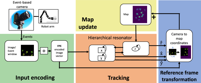
Figure 1: Neuromorphic Event-Based Visual Odometry with the Hierarchical Resonator Network. Events from an event-based camera are collected and encoded using fractional power encoding (FPE) into a VSA vector. The generative model assumes that the input is generated from a rotated and translated map. This model is inverted by the hierarchical resonator using two interacting partitions with different frames of reference. The translation ($\hat{x},\hat{y}$) and rotation ($\hat{r}$) estimates are then used to transform the input into map coordinates and to update the map.

Visual Odometry with the Hierarchical Resonator Network: Results

Following recent event-based visual odometry work [34, 35, 36, 37, 38, 39, 40], we use event-based data from the Event Camera Dataset [41] to benchmark our architecture. The dataset contains events, frames, and IMU measurements from a DAVIS240C event-based sensor and high-speed 6-DoF motion capture for the ground truth. We use the shapes_rotation sequence, which is 60 seconds long and was recorded while the camera was rotated by hand in 3 DoF in front of a wall with images of geometrical shapes. The data sequence contains almost no translation but very fast rotation (angular velocity up to 730^∘/s), which leads to motion blur and large jumps in the conventional camera frames but is well resolved by the DVS camera events.

For simplicity, we assume that the camera movement happens only in the three rotational DoF (roll, pan, and tilt) and approximate pan and tilt as pure translations in the pixel space. We show that the network is able to follow the camera movement faithfully with a median error of 3.5 degrees. As shown in Table 1, our VSA-based resonator network outperforms the neural networks trained on samples of the shapes_rotation dataset as reported by [38]. However, we would like to point out that [38] uses a small amount of training data. Larger amounts of data are likely to improve the performance and generalization of such models. Note that our approach does not require training. Instead, we calibrate the trajectories by using part of the data after the experiment to find the lag and linear transform that minimize the error to the ground truth. For this calibration, we use either the same split (70/30) as [38] (numbers given in parentheses) or just the last 10 seconds of the same training set, which yields better results with fewer data. This is likely due to the fact that it is closer to the test set and it provides a larger movement range per time, excluding the slow movements at the beginning of the recording.

Publication	Name	angle error (∘)
[42] Kendall et al. (2015) by [38]	PoseNet	12.5
[43] Kendall et al. (2016) by [38]	Bayesian PoseNet	12.1
[44] Laskar et al. (2017) by [38]	Pairwise-CNN	10.4
[45] Walch et al. (2017) by [38]	LSTM-Pose	7.6
[38] Nguyen et al. (2019)	SP-LSTM	5
Renner et al. (2022) (ours)	Neuromorphic VO	3.5 (4.7)
Renner et al. (2022) (ours)	Neuromorphic VO + IMU	2.7 (4.2)

Table 1: Comparison of different neural network architectures based on the median angular error for the shapes_rotation dataset. The given numbers from our work are obtained using only the last part of the training set from [38] for calibration. In parentheses are the errors when the whole training set is used.

The estimated camera trajectories compared to the ground truth are shown in Fig. 2. Fig.2A shows the unprocessed readout of the resonator states over several iterations at the beginning and the middle of the experiment. The inner product similarity of the resonator state with the VSA encoding vectors that code for the given locations is plotted. The states are initialized randomly so that the similarity is approximately equally distributed over all locations (left panels) in the beginning. In an orientation phase, in the first few iterations, the resonator quickly identifies several possible solutions that are active in superposition before the resonator starts tracking the correct camera trajectory a few iterations later.

From these similarity traces, we obtain the trajectories of the best estimates of the three output values by calculating a similarity-weighted mean of the indices in each iteration (see Eq. 8). Then we calibrate these trajectories and compare the trajectories to the ground truth, as shown in Fig. 2B. The network output and the ground truth match closely. The trajectory obtained from integrating (dead reckoning) the readings from the inertial measurement unit (IMU), which is also shown in Fig. 2B, drifts significantly, as expected from dead reckoning. In our VO network, drift is significantly smaller, as the movement is tracked relative to the map without dead reckoning.

The dynamic map at the end of the experiment is shown in Fig.2C. Fig.2D shows the input to the network (green) and the map transformed to the egocentric coordinates for visualization purposes at several points during the experiment. The first image is taken directly after the orientation phase when the overlap between the map and the input is perfect. The third image is taken around the iteration with the largest error. A likely reason for the increased error in this iteration is a combination of poor correspondence between the map and the current input and very fast camera movements that makes it hard to follow with the slower state update dynamics.

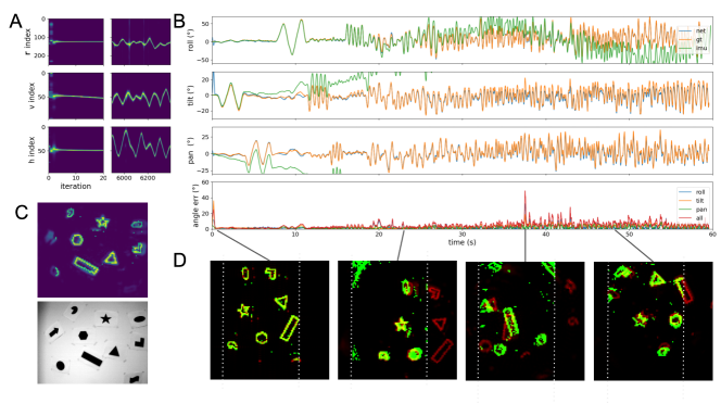
Figure 2: Tracking of the camera rotation from the event-based shapes_rotation dataset [41] in simulation. A. Unprocessed readout (inner product similarity) of the resonator states at the beginning of the experiment (left) and in later iterations around second 37.5 of the dataset (right). The r index directly corresponds to the roll angle while v and h are rotated and scaled (calibrated) into pan and tilt angles. Brighter colors indicate a higher inner product similarity of the resonator state with the codebook vector at the given location. After a short orientation phase where several locations are active in superposition, the states converge to a unique solution and follow the camera’s movement after less than ten iterations. In later iterations (right), we observe that the similarity peak also becomes broader (i.e., the network is less certain) when the camera moves quickly outside of the area covered by the map leading to increased error (as seen in B and D). B. Population vector readout (blue) of the angles calibrated to the ground truth coordinates. Ground truth from motion capture (orange). Camera trajectory from IMU measurement (green). Lowest row: plot of the tracking error (angle between ground truth and output trajectory) over time. C. Map at the end of the experiment (top) and conventional camera frame that shows the scene in its entirety (bottom). D. Event-based camera input (green) and transformed map (red) at 4 different iterations. Overlapping pixels between the map and camera view are yellow. The map was rotated and shifted by the current estimate of the network in order to show correspondence. White dotted lines indicate the borders of the camera image. The area outside of the white lines is zero-padded, as the transformed map can protrude the camera image

Sensory fusion of IMU and vision

To improve the performance of the network in situations when VO generates a large error and to emphasize the flexibility of our approach and the VSA framework, we demonstrate sensory fusion of the visual and inertial modalities in Fig. 3. While the visual odometry provides absolute angles relative to the map, the IMU measurements provide the angular velocities, i.e., the rates of change of the rotation angles. This means we can include a prediction step into the state update equations (see Eq. 11). Instead of just estimating each state from the input and the other states, each state is predicted using its rate of change before it is used to update the other states. As expected, the peak in the state readout becomes sharper in Fig. 3A compared to Fig. 2A, and particularly in difficult iterations, the error is significantly reduced, leading to an overall lower median error in this experiment of 2.7 degrees (see Tab. 1).

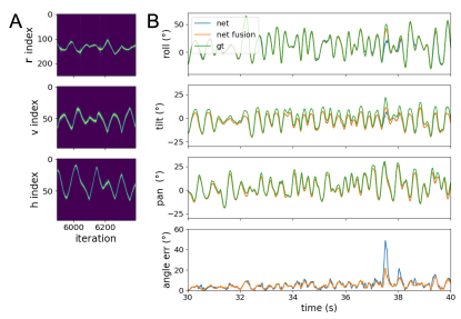
Figure 3: Tracking of the camera rotation from the event-based shapes_rotation dataset [41] in simulation using both IMU and event-based vision sensors. A. Unprocessed readout of the resonator states around second 37.5 of the dataset, for the network including IMU fusion, compare with Fig. 2A. B. Comparison of the trajectories and error with and without fusion. The network that uses both VO and IMU performs better in cases where VO is difficult.

Robust VO with a dynamic scene

To demonstrate the independence of the algorithm on the specific dataset and camera and to allow us to record a controlled dynamic scene, we built a custom setup using a robotic arm with an event-based camera mounted on the wrist. The arm was moved repeatedly in an arc over a static tabletop scene, as shown in Fig. 4A. The network tracks the camera’s movement relative to the starting position in three degrees of freedom (translation in the horizontal and vertical direction and roll angle). Here, the network achieves a median error of 1 cm in the position and 2.2 degrees in the roll angle. The error and the comparison with the ground truth are shown in Fig. 4.

For simplicity, our system assumes that scenes are planar and mostly static, i.e., the objects do not move. However, in reality, this assumption rarely holds. In future work, it is possible to include separate moving 3D objects in the generative model of the scene. However, in this proof of concept, we content ourselves with testing the robustness of our VO algorithm to dynamic changes in the scene by manually removing a large object, e.g., the bowl in Fig. 4A. Removal of the bowl does not increase the error significantly, and we visualize in Fig. 4C how the removed bowl vanishes from the dynamic map throughout the experiment.

So, the dynamic map update lends the network robustness to dynamic scene changes, and it allows the network to operate in regions of the scene not captured in the initial map. However, in longer simulations, there is a risk that the map (and, therefore, our navigation coordinate frame) drifts because the estimated transforms used for the map updates are not always accurate. To avoid such drift, we make the initial map a fixed point of the dynamics and thereby anchor the map. This is achieved by adding the initial map at each map update, as described in Eq. 10. The effect of this anchoring can be seen in Fig. 4D. The position variance is increased when the arm moves to the left, which is further away from the initial map. In future work, mechanisms for re-anchoring with a hierarchy of maps could be explored.

Figure 4: Tracking of the location and rotation of an event-based camera mounted on a robotic arm. A. The robotic arm setup and the tabletop scene with the event-based camera mounted on the arm. The arm moves back and forth in the arc shown in red. B. Population vector readout (blue) of the angles transformed to the ground truth coordinates. Ground truth from the robotic arm (orange). Lowest row: tracking error over time for location (left axis) and rotation (right axis). C. Tracking and mapping are robust against small changes in the scene. The map at the iteration before removal of the bowl, just after removal, and seconds after removal. As soon as the bowl is removed, it fades from the map until it is fully deleted. D. Population vector readout of the roll angle (color) and x, y locations transformed into the ground truth coordinate system.

Discussion

We developed a novel neuromorphic solution to visual odometry (VO), or self-motion estimation, – one of the fundamental tasks in robotics [2, 3]. We achieved state-of-the-art performance of the proposed VO algorithm on the event-based dataset [41], as well as demonstrated its applicability to a real-world robotic task. Our approach leverages VSAs, recently proposed as a framework for programming neuromorphic hardware [17]. Notably, the proposed solution combines three recent innovations in VSAs: (1) fractional power encoding [25, 27, 26] for encoding continuous quantities and transforms, (2) resonator networks [28, 29] for efficiently analyzing the visual input, and (3) phasor-based VSA models [22, 25] for enabling a neuromorphic implementation.

Neuromorphic computing holds great promise in terms of efficiency, as measured by the energy-delay product [10]. Designing algorithms for this unconventional computing architecture, however, is a challenge. Currently, most researchers use multi-layer artificial neural networks (ANNs) trained with deep learning on- or off-chip as a programming framework for neuromorphic chips. This framework parametrizes algorithms with artificial neurons, configured in layered, densely connected, feed-forward networks [46, 47, 48, 49]. Unsurprisingly, feed-forward processing with artificial neurons under-uses the capabilities of neuromorphic hardware to yield only modest gains over implementations in traditional computers or GPUs [10]. It is the exploitation of spike-timing, intrinsic neural dynamics, and recurrent architectures [10, 50, 51] that yield energy-delay products in neuromorphic hardware exceeding those in conventional computing hardware by orders of magnitudes [10].

A novel framework for neuromorphic computing hardware based on VSAs can overcome many limitations of the ANN framework [17]. In particular, real-valued VSAs, encoded with firing rates, have been used to design algorithms with spiking neurons on neuromorphic hardware for cognitive [52] and other tasks [15, 53, 54]. Unfortunately, a rate code requires many costly spikes per neuron. Our results showcase a new VSA-based computing framework for programming neural computations based on a spike-timing code. Specifically, we used a VSA with complex state vectors, called holographic reduced representations [21]. In our framework, the phase of a complex variable is encoded by the spike times of a rhythmically firing “phasor neuron” [22]. This allowed us to map the resonator network on neuromorphic hardware, specifically Intel’s research chip Loihi, as shown in the accompanying paper [23]. In order to scale the model and implement additional features, such as updates of the map, which are required for an implementation of the network presented here, we rely on the new features of Intel’s most recent Loihi 2, such as the programmable neuron model and graded spikes.

Computationally, our approach is related to previous work on spatial correlation-based approaches, particularly the map-seeking circuit (MSC) [55]. The map-seeking circuit is a multi-layer network with feedback that performs inference in generative models and has been successfully used for image registration in adaptive optics [56]. Our VO method shares with the MSC the use of superposition and content-addressable memory for estimating the transforms. The main differences are in the internal representations and computation. The MSC is based on standard ANN operations, while our approach uses the vector binding operation of VSAs. Accordingly, we avoid representing the transforms with large sets of matrices to tile the transform parameters at sufficiently fine resolution. The transforms are instead represented by VSA vectors of the same dimensionality as the encoded input.

Another neural solution of VO is based on deep learning. In this case, the mapping from the visual scene to the camera coordinates is stored in synaptic weights of a deep ANN. We have observed overfitting to the specific scene(s) used in training such deep ANNs in the examples that we used for comparison in this work, where both training and test sets were extracted from the same event sequence [38]. In contrast, our model holds the visual scene in the working memory of the dynamic map, not demanding generalization over all possible scenes in the trained weights, as in convolutional neural network approaches, such as [57]. We can easily change the tracked map or object, as demonstrated in the map update experiment. The resonator network is small compared to the convolutional approach - approximately in the order of 100k neurons vs. many millions with deep CNNs while performing similarly or better. In future work, our model could, however, be augmented with pre-trained CNNs for more detailed scene analysis. For instance, a CNN could be used to recognize or detect individual objects making the input to the resonator network even sparser (fewer events per point in space) than the one built directly from events of the dynamic vision sensor. With such preprocessing, the VSA could even better play out its strength which is representing and computing on sparse high-dimensional data. Furthermore, this could be a step toward semantic Simultaneous Localization and Mapping (SLAM).

To put this work in a broader context, we note that in the last decade, significant progress has been made in performing visual odometry tasks with event-based cameras [58, 59, 60, 61, 62, 63, 64, 65, 66, 67, 68]. The use of event-based cameras enables high temporal resolution ($>1kHz$) with reduced motion blur at a lower computational cost compared to high-speed cameras, and it is robust to light intensity changes. Our algorithm shares these advantages and can save time and energy compared to conventional computing approaches, as we can make use of parallel in-memory processing. Efficient solutions to VO are crucial for energy-constrained robotics applications such as small autonomous drones [4] and planetary rovers [5, 6, 7].

In its current form, the model serves as a validation of the VSA and hierarchical resonator approach in a robotics task. It is, however, still a limited demonstration of the framework’s capability, as we considered a 2-dimensional scene at a fixed distance both in our robotic setup and the dataset benchmark. Scaling this architecture to a fully-fledged 3D scenario with a 6 degree of freedom motion estimation requires further extensions of the hierarchical resonator theory and likely the inclusion of additional modalities or stereo vision. We have shown that integrating additional sensor channels, such as an inertial measurement for motion estimation, leads to more effective and precise multi-modal odometry. In future work, this approach could be extended with depth perception, e.g., with stereo or LIDAR technology. The resonator framework and VSA representations are well-suited for fusion of different sensory modalities due to their use of homogeneous vector-based representations for different spaces and transformations between them.

Methods

.1 Data and preprocessing

Event camera dataset.

The event-based dataset [41] that we used in our validation experiment contains events and IMU measurements from a DAVIS240C camera [69] and high-speed 6-DoF motion-capture for the ground truth. The shapes_rotation sequence is 60 seconds long and was recorded holding the camera in hand and rotating it in 3 rotational degrees of freedom. It contains almost no translation but very fast rotation (angular velocity up to $730^{\circ}/s$).

Robotic arm setup.

We ran another set of experiments to demonstrate VO with an event-based camera mounted on a robotic arm. We used a Prophesee event-based camera evaluation kit for the experiment: an event-based vision sensor with VGA resolution (640x480), a C mount lens (70 degrees FOV), and Prophesee player software. A Prophesee Gen2 Metavision event-based camera was mounted on a Jaco2 robot arm - specifically, on the joint that meets the end-effector - using a wristband (see Fig. 4). The Jaco2 arm is a 6DoF assistive robot arm. The arm is mounted on a table with several objects, including a cup, utensils, and bowl, placed on top to simulate real-world use cases (see Fig. 4A). The robot arm’s reach is 90 cm, and it is mounted on the platform next to the table of size 75cm x 75cm.

We moved the arm in the 2D plane with the camera facing down, scanning the table. We recorded the data using the Prophesee player software. We used the Kinova Jaco2 and custom-built software to control the arm and record its trajectory.

DVS data preprocessing

For all network simulations, recorded events were used. Events were stored with a timestamp, pixel coordinates (x, y), and a polarity (on/off). Polarity was discarded. Coordinates were downsampled from 640x480 to 64x48 pixels for the Prophesee sensor and from 240x180 to 96x72 pixels for the INIvation DAVIS240C. This was achieved by dividing the event coordinates by the respective factor and then rounding them to integers. For the shapes_rotation dataset, a fixed amount of 2000 events, and for the robotic arm dataset, 5000 events were accumulated into one event package (set of events), which makes the processing mostly invariant to the current movement speed. Especially for faster movements, even smaller packages would be possible and yield a better temporal resolution. Finally, a binary array $I$ was created by setting all pixels with more than 0 (shapes_rotation) or 1 (robotic arm) events to 1 and all others to 0, effectively removing some noise events in the latter case.

.2 Encoding

Throughout this paper, we use the Fourier Holographic Reduced Representations (FHRR) VSA [70, 21], which uses vectors of complex numbers like the Fourier transform. We use fractional power encoding (FPE) [70, 25, 27, 26] to represent space, as described in [23]. In this vector encoding, space is spanned by repeated binding of a VSA “seed vector”, while the binding operation is generalized to fractions so that it can be applied on a continuous scale [70, 25, 27, 26]. Instead of synthetic images of letters, as in [23], we encoded an event package into a VSA vector. With FPE, a set of events $s$ can be encoded as the sum of the exponentiated seed vectors $h_{0}$ and $v_{0}$ (for horizontal and vertical coordinates):

$$\mathbf{s} =\sum_{x,y\text{ in }E}{\mathbf{h}_{0}^{x}\odot\mathbf{v}_{0}^{y}},$$ (1)

Here, the sum denotes bundling, which is the sum of complex numbers, and $\odot$ signifies binding, which is the element-wise (Hadamard) product. For instance, a set of 3 events ($E=\{[27,24],[39,43],[28,38]\}$) is encoded as follows:

$$\mathbf{s} =\mathbf{h}_{0}^{27}\odot\mathbf{v}_{0}^{24}+\mathbf{h}_{0}^{39}\odot\mathbf{v}_{0}^{43}+\mathbf{h}_{0}^{28}\odot\mathbf{v}_{0}^{38}.$$ (2)

In practice, as long as the possible ranges of x and y are known beforehand, which is the case for camera pixels, the encoding can also be written as a matrix product of the complex codebook matrix $\Phi$ and the binary event array I. The codebook matrix contains a codebook vector for each pixel location $[x,y]$ that is calculated by $\mathbf{h}_{0}^{x}\odot\mathbf{h}_{0}^{y}$. In this formulation, the event package can be encoded by:

$$\mathbf{s} =\Phi I.$$ (4)

The FPE encoding constitutes a generalization of the Fourier transform. In the case of regularly spaced seed vector phases containing all N $N^{th}$-roots of unity, the 1D FPE becomes equivalent to a 1D Fourier transform. In the 2D case described above, $\Phi$ would be the DFT matrix. This can be used to achieve equivariance of the binding operation with periodic transformations, such as rotation. A similar mechanism to encode event-based vision pixels into a hyperdimensional vector was employed by [71] using permutations instead of binding with the Hadamard product. The error reported for the shapes_rotation dataset and the trajectories shown in Fig. 2 were obtained using the regular DFT codebook matrix. The trajectory in Fig. 4 was obtained using a random codebook matrix with a vector size of N = 3072.

.3 Network architecture

As shown in Fig. 1, the network can be split into three parts: (1) The hierarchical resonator that performs the tracking, (2) the reference frame transformation from the camera to the map coordinates, and (3) the map update. The hierarchical resonator receives the encoded image and the map as input and outputs estimates of the transformation between the two inputs. The next module uses these estimates to transform the encoded input image from the camera to map coordinates. This transformed image in map coordinates is then used to update the map.

The resonator network was introduced in [28]. Here, we use the hierarchical resonator network [23] that generalizes the resonator by allowing a nested structure of factors that can use different reference frames (such as log-polar coordinates). The version used here is simpler than in [23], as we do not include color and scale. Furthermore, we only have a single template, which we call map in this paper. However, unlike in [23], the map changes over time, and the input to the network is not a static artificial letter but a stream of events from a DVS camera.

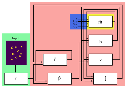
Figure 5: Hierarchical resonator for visual odometry. Colors match Fig.1. The dynamics are explained in Eq.5.

The evolution of the three states of the resonator network (horizontal displacement $h$, vertical displacement $v$, and rotation $r$) is described by the following equations and visualized in Fig. 5:

$$\begin{split}\mathbf{\hat{h}}(t+1)&=(1-\gamma)\mathbf{\hat{h}}(t)+\gamma f\Big{(}\mathbf{H}p\Big{(}\mathbf{H}^{\dagger}\Big{(}\mathbf{\hat{p}}(t)\odot\mathbf{\hat{v}}^{*}(t)\odot\mathbf{\hat{m}}^{*}(t)\Big{)}\Big{)}\Big{)},\\ \mathbf{\hat{v}}(t+1)&=(1-\gamma)\mathbf{\hat{v}}(t)+\gamma f\Big{(}\mathbf{V}p\Big{(}\mathbf{V}^{\dagger}\Big{(}\mathbf{\hat{p}}(t)\odot\mathbf{\hat{h}}^{*}(t)\odot\mathbf{\hat{m}}^{*}(t)\Big{)}\Big{)}\Big{)},\\ \mathbf{\hat{r}}(t+1)&=(1-\gamma)\mathbf{\hat{r}}(t)+\gamma f\Big{(}\mathbf{R}p\Big{(}\mathbf{R}^{\dagger}\Big{(}\mathbf{s}(t)\odot\mathbf{\hat{l}}^{*}(t)\Big{)}\Big{)}\Big{)},\\ \text{with}\\ \mathbf{\hat{p}}(t)&=\mathbf{\Lambda}\big{(}\mathbf{s}(t)\odot\mathbf{\hat{r}}^{*}(t)\big{)},\\ \mathbf{\hat{l}}(t)&=\mathbf{\Lambda}^{-1}\big{(}\mathbf{\hat{m}}\odot\mathbf{\hat{h}}^{*}(t)\odot\mathbf{\hat{v}}^{*}(t)\big{)}.\end{split}$$ (5)

$\mathbf{s}(t)$ is the input as obtained from Eq. 4. The letters with the $\hat{}$ are the current states of the resonator at a given iteration t. The capital letters ($H,V,R$) are the encoding matrices for the respective states ($h,v,r$). The encoding matrices are created by generating a codebook vector for each location using FPE. Cleanup of the state is achieved by first decoding the state with the complex conjugate transpose ($\dagger$) of the encoding matrix, taking the real value and applying an optional nonlinearity, and then encoding it again by a matrix product with the encoding matrix. $f$ denotes a nonlinearity, specifically, elementwise division of the complex vector by the complex magnitudes, i.e., projection to the unit circle in the Gaussian number plane. $p$ is another nonlinearity that leads to a stronger cleanup: $p(\mathbf{x})=\mathbf{x}^{k}/|\mathbf{x}^{k}|_{2}$, with $k$ typically being between 2 and 20. $\Lambda$ denotes the matrix that transforms between the VSA vector in Cartesian coordinates and the one in polar or log-polar coordinates. $\gamma$ is constant (0.2) and determines the speed of the state update. $*$ denotes the complex conjugate necessary for unbinding of a state. Note that if binding corresponds to a shift in one direction, unbinding corresponds to the same shift but in the opposite direction.

The readout of the resonator is done as follows: First, the state is decoded using the decoding matrix. This corresponds to calculating the inner product similarity of the resonator state with the codebook vectors at each location of interest. To get the best locations, one could take the index with the largest similarity value. This, however, discards much of the information contained in the similarity distribution (see Fig. 2A and Fig. 3 for plots of this unprocessed state readout). Therefore the output of the network is calculated as a population vector of the state readout (similar to [72]). The population vector is the similarity-weighted average of the indices (see Eq. 8). It allows sub-pixel (sub-index) resolution compared to simply taking the index of the largest value. To avoid the influence of outliers, only the five neighboring indices on both sides of the index with the largest value were used for the population vector decoding. I.e., first, the highest peak in the readout is selected, then the neighborhood around the peak is used to determine the exact estimate.

For instance, for the horizontal (h) state, the network output is calculated as follows:

$$h_{dec}(t)=H^{\dagger}\mathbf{\hat{h}}(t),$$ (6)

$$h^{max}_{dec}=argmax(h_{dec}(t)),$$ (7)

$$h_{out}(t)=\frac{\sum_{i=[h^{max}_{dec}-5,h^{max}_{dec}+5]}{ih_{dec,i}(t)}}{\sum_{i=[h^{max}_{dec}-5,h^{max}_{dec}+5]}{h_{dec,i}(t)}}.$$ (8)

The map estimate $\hat{m}$ is treated almost like a regular resonator state. However, a cleanup matrix does not exist, as the map is not known beforehand and changes over time. Unlike the other states, which are initialized by a random complex vector of unit magnitude, the first map $\hat{m}(0)$ is the first input $s(0)$ to the network. This means that all transformations will be relative to this starting position, and the origin of the map reference frame is set to be at the origin of this first map. After that, the map is updated (Eq. 10) similarly to the other states by an estimate created from the other states. This estimate is the input rotated and shifted from input to map coordinates, see Eq. 9). This transformation could, in principle, be performed using the cleaned-up resonator states. However, to achieve a cleaner map, the update is performed using the output of the network, i.e., only with the best transformation estimate (i.e., the network output as described in Eq. 8) instead of a superposition of all likely transformations as needed for the resonator.

As described in Eq. 9, the transformation of the map is performed using fractional binding of the current input vector $s(t)$ with the seed vectors exponentiated by the real-valued output of the network.

To avoid a wrong map update, which could lead to a remapping to a different frame of reference, the map update is blocked during the first 100 iterations (after which the correct transformation has usually been found).

To avoid drifts of the map that can happen if the estimates are slightly off over a longer time, the map is anchored to the starting map. This is achieved by adding the starting map $\hat{m}(0)$ to the map update at each iteration with a low weight $\mu_{2}$. Here, the anchor is the first map that defines the navigation frame and does not change; however, the anchor could also be implemented as a slowly updating long-term memory.

$$\mathbf{m}(t) =\big{[}\mathbf{\Lambda}\big{(}\mathbf{s(t)}\odot\mathbf{h}^{h_{out}(t)}\odot\mathbf{v}^{v_{out}(t)}\big{)}\big{]}\odot\mathbf{r}^{r_{out}(t)},$$ (9)

$$\mathbf{\hat{m}}(t+1) =\mu_{1}\mathbf{\hat{m}}(t)+\mu_{2}\mathbf{\hat{m}}(0)+(1-\mu_{1}-\mu_{2})\mathbf{m}(t).$$ (10)

For the IMU fusion experiments, the states are additionally updated before every resonator iteration using fractional binding with the IMU reading from the shapes_rotation dataset, interpolated to the current timestamp, and adjusted to the time difference between the current and the last timestamp.

For instance, the roll angle estimate $\hat{r}$ is updated as follows:

$$\mathbf{\hat{r}}(t)=\mathbf{\hat{r}}(t-1)\odot r^{r_{IMU}(t)},$$ (11)

where $r$ is the seed vector for the roll angle and $r_{IMU}(t)$ is the IMU reading interpolated at time t.

.4 Analysis

For the comparison with the ground truth, we obtained the raw state trajectory over time by decoding the states by the population vector readout explained above for each iteration. Each iteration was assigned the timestamp in the middle of the first and last event of the respective event package processed in that iteration. To determine the lag, we resampled the ground truth and the raw output trajectory to a fixed sampling rate of 400 Hz using linear interpolation. Finally, we calculated the lag between the ground truth and the network by crosscorrelation of the camera roll trajectory.

To determine the error, the ground truth trajectories were resampled using linear interpolation to the timestamps of the network trajectories. A part of the trajectories was used to find the best matching scaling, translation, and rotation using the Umeyama algorithm for rigid alignment [73] to calibrate the pan and tilt (or horizontal and vertical) trajectories. For the shapes_rotation dataset, we used either the same 70/30 dataset split (called ”novel split”) as [38] or we only used the last 10 seconds of the training set for calibration. We used the first arc ($0.5-5s$) for the robotic arm data. This calibration is needed as the ground truth reference frame is not necessarily the same as the first map reference frame. Also, the network calculates the translation in pixel coordinates. The roll angle was set to start at 0 but is not calibrated as the network output is in absolute angles like the ground truth. Note that the calibration maps the network’s v and h output traces to pan and tilt angles in case of the shapes_rotation data and to x and y positions in case of the robotic arm data.

The code in this work was written in python 3.8. Preprocessing and simulations were conducted using NumPy, and plots were generated with matplotlib. We used SciPy for interpolation and the python package quaternion for processing the ground truth trajectory of the shapes dataset.

Author Contributions

All authors contributed to writing and editing; YS and LS conceptualized the project in the robotic space; PF and FS provided guidance on the new VSA approach; AR developed the VO network model, implemented, ran, and analyzed the network simulations; LS design and ran the robotic arm experiments.

References

References

- [1] M. Srinivasan, “Honey bees as a model for vision, perception, and cognition,” Annual Review of Entomology, vol. 55, pp. 267–284, 2010.
- [2] D. Nistér, O. Naroditsky, and J. Bergen, “Visual odometry,” in Proceedings of the 2004 IEEE Computer Society Conference on Computer Vision and Pattern Recognition, 2004. CVPR 2004., vol. 1, pp. I–I, Ieee, 2004.
- [3] D. Scaramuzza and F. Fraundorfer, “Visual odometry [tutorial],” IEEE robotics & automation magazine, vol. 18, no. 4, pp. 80–92, 2011.
- [4] D. Palossi, A. Loquercio, F. Conti, E. Flamand, D. Scaramuzza, and L. Benini, “A 64-mW DNN-based visual navigation engine for autonomous nano-drones,” IEEE Internet of Things Journal, vol. 6, pp. 8357–8371, oct 2019.
- [5] H. P. Moravec, Obstacle avoidance and navigation in the real world by a seeing robot rover. PhD thesis, Stanford University, 1980.
- [6] S. Lacroix, A. Mallet, R. Chatila, and L. Gallo, “Rover self localization in planetary-like environments,” in Artificial Intelligence, Robotics and Automation in Space, vol. 440, p. 433, 1999.
- [7] P. Corke, D. Strelow, and S. Singh, “Omnidirectional visual odometry for a planetary rover,” in 2004 IEEE/RSJ International Conference on Intelligent Robots and Systems (IROS)(IEEE Cat. No. 04CH37566), vol. 4, pp. 4007–4012, IEEE, 2004.
- [8] C. Mead, “Neuromorphic electronic systems,” Proceedings of the IEEE, vol. 78, no. 10, pp. 1629–1636, 1990.
- [9] G. Indiveri, B. Linares-Barranco, T. J. Hamilton, A. van Schaik, R. Etienne-Cummings, T. Delbruck, S.-C. Liu, P. Dudek, P. Häfliger, S. Renaud, J. Schemmel, G. Cauwenberghs, J. Arthur, K. Hynna, F. Folowosele, S. Saighi, T. Serrano-Gotarredona, J. Wijekoon, Y. Wang, and K. Boahen, “Neuromorphic silicon neuron circuits.,” Frontiers in Neuroscience, vol. 5, p. 73, may 2011.
- [10] M. Davies, A. Wild, G. Orchard, Y. Sandamirskaya, G. A. F. Guerra, P. Joshi, P. Plank, and S. R. Risbud, “Advancing neuromorphic computing with loihi: A survey of results and outlook,” Proceedings of the IEEE, pp. 1–24, 2021.
- [11] S.-C. L. Giacomo Indiveri, “Memory and information processing in neuromorphic systems.,” PROCEEDINGS OF THE IEEE, vol. 103, pp. 1379–1397, june 2015.
- [12] T. A. Plate, “Analogy Retrieval and Processing with Distributed Vector Representations,” Expert Systems: The International Journal of Knowledge Engineering and Neural Networks, vol. 17, no. 1, pp. 29–40, 2000.
- [13] R. Gayler, “Multiplicative binding, representation operators & analogy (workshop poster).,” (Sofia), New Bulgarian University, 1998.
- [14] P. Kanerva, “Binary Spatter-Coding of Ordered K-tuples,” in International Conference on Artificial Neural Networks (ICANN), vol. 1112 of Lecture Notes in Computer Science, pp. 869–873, 1996.
- [15] C. Eliasmith and C. H. Anderson, Neural engineering: Computation, representation, and dynamics in neurobiological systems. MIT press, 2003.
- [16] Y. Sandamirskaya, “Dynamic neural fields as a step toward cognitive neuromorphic architectures.,” Frontiers in Neuroscience, vol. 7, p. 276, 2013.
- [17] D. Kleyko, M. Davies, E. P. Frady, et al., “Vector Symbolic Architectures as a Computing Framework for Nanoscale Hardware,” arXiv:2106.05268, pp. 1–28, 2021.
- [18] D. Liang, R. Kreiser, C. Nielsen, N. Qiao, Y. Sandamirskaya, and G. Indiveri, “Neural state machines for robust learning and control of neuromorphic agents,” IEEE Journal on Emerging and Selected Topics in Circuits and Systems, vol. 9, no. 4, pp. 679–689, 2019.
- [19] R. W. Gayler, “Vector Symbolic Architectures Answer Jackendoff’s Challenges for Cognitive Neuroscience,” in Joint International Conference on Cognitive Science (ICCS/ASCS), pp. 133–138, 2003.
- [20] P. Kanerva, “Hyperdimensional computing: An introduction to computing in distributed representation with high-dimensional random vectors,” Cognitive computation, vol. 1, pp. 139–159, jun 2009.
- [21] T. A. Plate, “Holographic reduced representations,” IEEE Transactions on Neural networks, vol. 6, no. 3, pp. 623–641, 1995.
- [22] E. P. Frady and F. T. Sommer, “Robust computation with rhythmic spike patterns.,” Proceedings of the National Academy of Sciences of the United States of America, vol. 116, pp. 18050–18059, sep 2019.
- [23] A. Renner, L. Supic, A. Danielescu, G. Indiveri, B. A. Olshausen, Y. Sandamirskaya, F. T. Sommer, and E. P. Frady, “Neuromorphic visual scene understanding with resonator networks,” arXiv preprint arXiv:2208.12880, 2022.
- [24] A. Noest, “Phasor neural networks.,” Neural information processing systems, p. 584, 1988.
- [25] P. Frady, P. Kanerva, and F. Sommer, “A framework for linking computations and rhythm-based timing patterns in neural firing, such as phase precession in hippocampal place cells,” CCN, 2019.
- [26] E. Frady, D. Kleyko, C. Kymn, B. Olshausen, and F. Sommer, “Computing on functions using randomized vector representations.,” arXiv preprint arXiv:2109.03429, 2021.
- [27] B. Komer, T. Stewart, A. Voelker, and C. Eliasmith, “A neural representation of continuous space using fractional binding.,” in Annual Meeting of the Cognitive Science Society (CogSci), pp. 2038–2043, Cognitive Science Society, 2019.
- [28] E. P. Frady, S. J. Kent, B. A. Olshausen, and F. T. Sommer, “Resonator networks, 1: An efficient solution for factoring high-dimensional, distributed representations of data structures.,” Neural Computation, pp. 1–21, oct 2020.
- [29] S. J. Kent, E. P. Frady, F. T. Sommer, and B. A. Olshausen, “Resonator networks, 2: Factorization performance and capacity compared to optimization-based methods.,” Neural Computation, vol. 32, pp. 2332–2388, dec 2020.
- [30] D. Casasent and D. Psaltis, “Position, rotation, and scale invariant optical correlation,” Applied optics, vol. 15, no. 7, pp. 1795–1799, 1976.
- [31] Q.-s. Chen, M. Defrise, and F. Deconinck, “Symmetric phase-only matched filtering of fourier-mellin transforms for image registration and recognition,” IEEE Transactions on pattern analysis and machine intelligence, vol. 16, no. 12, pp. 1156–1168, 1994.
- [32] B. S. Reddy and B. N. Chatterji, “An fft-based technique for translation, rotation, and scale-invariant image registration,” IEEE transactions on image processing, vol. 5, no. 8, pp. 1266–1271, 1996.
- [33] G. Gallego, T. Delbrück, G. Orchard, C. Bartolozzi, B. Taba, A. Censi, S. Leutenegger, A. J. Davison, J. Conradt, K. Daniilidis, et al., “Event-based vision: A survey,” IEEE transactions on pattern analysis and machine intelligence, vol. 44, no. 1, pp. 154–180, 2020.
- [34] C. Reinbacher, G. Munda, and T. Pock, “Real-time panoramic tracking for event cameras,” in 2017 IEEE International Conference on Computational Photography (ICCP), pp. 1–9, IEEE, may 2017.
- [35] H. Rebecq, T. Horstschaefer, and D. Scaramuzza, “Real-time visual-inertial odometry for event cameras using keyframe-based nonlinear optimization,” in Procedings of the British Machine Vision Conference 2017, p. 16, British Machine Vision Association, 2017.
- [36] A. Zihao Zhu, N. Atanasov, and K. Daniilidis, “Event-based visual inertial odometry,” in Proceedings of the IEEE Conference on Computer Vision and Pattern Recognition, pp. 5391–5399, 2017.
- [37] A. R. Vidal, H. Rebecq, T. Horstschaefer, and D. Scaramuzza, “Ultimate slam? combining events, images, and imu for robust visual slam in hdr and high-speed scenarios,” IEEE Robotics and Automation Letters, vol. 3, no. 2, pp. 994–1001, 2018.
- [38] A. Nguyen, T.-T. Do, D. G. Caldwell, and N. G. Tsagarakis, “Real-time 6DOF pose relocalization for event cameras with stacked spatial LSTM networks,” in 2019 IEEE/CVF Conference on Computer Vision and Pattern Recognition Workshops (CVPRW), pp. 1638–1645, IEEE, jun 2019.
- [39] H. Rebecq, R. Ranftl, V. Koltun, and D. Scaramuzza, “High speed and high dynamic range video with an event camera,” IEEE transactions on pattern analysis and machine intelligence, 2019.
- [40] K. Xiao, G. Wang, Y. Chen, Y. Xie, and H. Li, “Research on event accumulator settings for event-based slam,” arXiv preprint arXiv:2112.00427, 2021.
- [41] E. Mueggler, H. Rebecq, G. Gallego, T. Delbruck, and D. Scaramuzza, “The event-camera dataset and simulator: Event-based data for pose estimation, visual odometry, and slam,” The International Journal of Robotics Research, vol. 36, no. 2, pp. 142–149, 2017.
- [42] A. Kendall, M. Grimes, and R. Cipolla, “PoseNet: A convolutional network for real-time 6-DOF camera relocalization,” in 2015 IEEE International Conference on Computer Vision (ICCV), pp. 2938–2946, IEEE, dec 2015.
- [43] A. Kendall and R. Cipolla, “Modelling uncertainty in deep learning for camera relocalization,” in 2016 IEEE International Conference on Robotics and Automation (ICRA), pp. 4762–4769, IEEE, may 2016.
- [44] Z. Laskar, I. Melekhov, S. Kalia, and J. Kannala, “Camera relocalization by computing pairwise relative poses using convolutional neural network,” in 2017 IEEE International Conference on Computer Vision Workshops (ICCVW), pp. 920–929, IEEE, oct 2017.
- [45] F. Walch, C. Hazirbas, L. Leal-Taixe, T. Sattler, S. Hilsenbeck, and D. Cremers, “Image-based localization using LSTMs for structured feature correlation,” in 2017 IEEE International Conference on Computer Vision (ICCV), pp. 627–637, IEEE, oct 2017.
- [46] S. Esser, P. Merolla, J. Arthur, A. Cassidy, R. Appuswamy, A. Andreopoulos, D. Berg, J. McKinstry, T. Melano, D. Barch, C. di Nolfo, D. P., A. Amir, B. Taba, M. Flickner, and D. Modha, “Convolutional networks for fast, energy-efficient neuromorphic computing,” PNAS, vol. 113, pp. 11441–11446, 2016.
- [47] C. Frenkel, M. Lefebvre, J.-D. Legat, and D. Bol, “A 0.086-mm 212.7-pj/sop 64k-synapse 256-neuron online-learning digital spiking neuromorphic processor in 28-nm cmos,” IEEE transactions on biomedical circuits and systems, vol. 13, no. 1, pp. 145–158, 2018.
- [48] S. B. Shrestha and G. Orchard, “Slayer: Spike layer error reassignment in time,” in Advances in Neural Information Processing Systems, pp. 1412–1421, 2018.
- [49] A. Renner, F. Sheldon, A. Zlotnik, L. Tao, and A. Sornborger, “The backpropagation algorithm implemented on spiking neuromorphic hardware,” arXiv preprint arXiv:2106.07030, 2021.
- [50] M. Davies, N. Srinivasa, T.-H. Lin, G. Chinya, Y. Cao, S. H. Choday, G. Dimou, P. Joshi, N. Imam, S. Jain, et al., “Loihi: A neuromorphic manycore processor with on-chip learning,” IEEE Micro, vol. 38, no. 1, pp. 82–99, 2018.
- [51] E. P. Frady, G. Orchard, D. Florey, N. Imam, R. Liu, J. Mishra, J. Tse, A. Wild, F. T. Sommer, and M. Davies, “Neuromorphic nearest neighbor search using intel’s pohoiki springs,” in Proceedings of the Neuro-inspired Computational Elements Workshop, (New York, NY, USA), pp. 1–10, ACM, mar 2020.
- [52] C. Eliasmith, T. C. Stewart, X. Choo, T. Bekolay, T. DeWolf, Y. Tang, and D. Rasmussen, “A large-scale model of the functioning brain.,” Science, vol. 338, pp. 1202–1205, nov 2012.
- [53] A. Mundy, J. Knight, T. C. Stewart, and S. Furber, “An efficient spinnaker implementation of the neural engineering framework,” in 2015 International Joint Conference on Neural Networks (IJCNN), pp. 1–8, IEEE, 2015.
- [54] F. Corradi, C. Eliasmith, and G. Indiveri, “Mapping arbitrary mathematical functions and dynamical systems to neuromorphic vlsi circuits for spike-based neural computation,” in 2014 IEEE International Symposium on Circuits and Systems (ISCAS), pp. 269–272, IEEE, 2014.
- [55] D. W. Arathorn, Map-seeking circuits in visual cognition: A computational mechanism for biological and machine vision. Stanford University Press, 2002.
- [56] C. R. Vogel, D. W. Arathorn, A. Roorda, and A. Parker, “Retinal motion estimation in adaptive optics scanning laser ophthalmoscopy,” Optics express, vol. 14, no. 2, pp. 487–497, 2006.
- [57] R. Serrano-Gotarredona, M. Oster, P. Lichtsteiner, A. Linares-Barranco, R. Paz-Vicente, F. Gomez-Rodriguez, L. Camunas-Mesa, R. Berner, M. Rivas-Perez, T. Delbruck, S.-C. Liu, R. Douglas, P. Hafliger, G. Jimenez-Moreno, A. Civit Ballcels, T. Serrano-Gotarredona, A. J. Acosta-Jimenez, and B. Linares-Barranco, “CAVIAR: a 45k neuron, 5M synapse, 12G connects/s AER hardware sensory-processing- learning-actuating system for high-speed visual object recognition and tracking.,” IEEE Transactions on Neural Networks, vol. 20, pp. 1417–1438, sep 2009.
- [58] M. Cook, L. Gugelmann, F. Jug, C. Krautz, and A. Steger, “Interacting maps for fast visual interpretation,” in The 2011 International Joint Conference on Neural Networks, pp. 770–776, IEEE, jul 2011.
- [59] H. Kim, A. Handa, R. Benosman, S.-H. Ieng, and A. Davison, “Simultaneous mosaicing and tracking with an event camera,” in Proceedings of the British Machine Vision Conference 2014, pp. 26.1–26.12, British Machine Vision Association, 2014.
- [60] E. Mueggler, B. Huber, and D. Scaramuzza, “Event-based, 6-DOF pose tracking for high-speed maneuvers,” in 2014 IEEE/RSJ International Conference on Intelligent Robots and Systems, pp. 2761–2768, IEEE, sep 2014.
- [61] A. Censi and D. Scaramuzza, “Low-latency event-based visual odometry,” in 2014 IEEE International Conference on Robotics and Automation (ICRA), pp. 703–710, IEEE, may 2014.
- [62] D. Weikersdorfer, D. B. Adrian, D. Cremers, and J. Conradt, “Event-based 3D SLAM with a depth-augmented dynamic vision sensor,” in 2014 IEEE International Conference on Robotics and Automation (ICRA), pp. 359–364, IEEE, may 2014.
- [63] G. Gallego, C. Forster, E. Mueggler, and D. Scaramuzza, “Event-based camera pose tracking using a generative event model.,” arXiv preprint arXiv:1510.01972, 2015.
- [64] B. Kueng, E. Mueggler, G. Gallego, and D. Scaramuzza, “Low-latency visual odometry using event-based feature tracks,” in 2016 IEEE/RSJ International Conference on Intelligent Robots and Systems (IROS), pp. 16–23, IEEE, oct 2016.
- [65] H. Rebecq, G. Gallego, E. Mueggler, and D. Scaramuzza, “EMVS: Event-based multi-view Stereo—3D reconstruction with an event camera in real-time,” International journal of computer vision, vol. 126, pp. 1–21, nov 2017.
- [66] H. Rebecq, T. Horstschäfer, G. Gallego, and D. Scaramuzza, “Evo: A geometric approach to event-based 6-dof parallel tracking and mapping in real time,” IEEE Robotics and Automation Letters, vol. 2, no. 2, pp. 593–600, 2016.
- [67] G. Gallego, H. Rebecq, and D. Scaramuzza, “A unifying contrast maximization framework for event cameras, with applications to motion, depth, and optical flow estimation,” in Proceedings of the IEEE Conference on Computer Vision and Pattern Recognition, pp. 3867–3876, 2018.
- [68] A. Z. Zhu, L. Yuan, K. Chaney, and K. Daniilidis, “Unsupervised event-based learning of optical flow, depth, and egomotion,” in 2019 IEEE/CVF Conference on Computer Vision and Pattern Recognition (CVPR), pp. 989–997, IEEE, jun 2019.
- [69] C. Brandli, R. Berner, M. Yang, S.-C. Liu, and T. Delbruck, “A 240 x 180 130 dB 3 us latency global shutter spatiotemporal vision sensor,” IEEE Journal of Solid-State Circuits, vol. 49, pp. 2333–2341, oct 2014.
- [70] T. Plate, Distributed representations and nested compositional structure. University of Toronto, Department of Computer Science, 1994.
- [71] A. Mitrokhin, P. Sutor, C. Fermüller, and Y. Aloimonos, “Learning sensorimotor control with neuromorphic sensors: Toward hyperdimensional active perception.,” Science Robotics, vol. 4, may 2019.
- [72] A. Renner, M. Evanusa, and Y. Sandamirskaya, “Event-based attention and tracking on neuromorphic hardware,” in 2019 IEEE/CVF Conference on Computer Vision and Pattern Recognition Workshops (CVPRW), pp. 1709–1716, IEEE, jun 2019.
- [73] S. Umeyama, “Least-squares estimation of transformation parameters between two point patterns,” IEEE Transactions on Pattern Analysis & Machine Intelligence, vol. 13, no. 04, pp. 376–380, 1991.