Intersection Numbers from Higher-order Partial Differential Equations

Abstract

We propose a new method for the evaluation of intersection numbers for twisted meromorphic $n$-forms, through Stokes’ theorem in $n$ dimensions. It is based on the solution of an $n$-th order partial differential equation and on the evaluation of multivariate residues. We also present an algebraic expression for the contribution from each multivariate residue. We illustrate our approach with a number of simple examples from mathematics and physics.

1 Introduction

The intersection number of differential $n$-forms matsumoto1994 ; matsumoto1998 ; OST2003 ; doi:10.1142/S0129167X13500948 ; goto2015 ; goto2015b ; Yoshiaki-GOTO2015203 ; Mizera:2017rqa ; matsubaraheo2019algorithm ; Ohara98intersectionnumbers ; https://doi.org/10.48550/arxiv.2006.07848 ; https://doi.org/10.48550/arxiv.2008.03176 ; https://doi.org/10.48550/arxiv.2104.12584 acts like an inner product in the de Rham twisted cohomology group, namely the quotient space of the closed forms modulo the exact forms, and therefore, it yields the decomposition of differential forms in a basis of forms, generating the vector space Mastrolia:2018uzb ; Frellesvig:2019kgj ; Frellesvig:2019uqt ; Frellesvig:2020qot .

A wide class of integral functions, such as Aomoto-Gel’fand integrals, Euler-Mellin integrals, Gel’fand-Kapranov-Zelevinsky integrals, to name a few, which embed and generalise Feynman integrals, can be considered as the pairing of regulated integration domains, known as twisted cycles, and of regulated forms, known as twisted cocycles aomoto2011theory . Within this definition, the integrand appears as the product of a multivalued function, called twist, and of a differential form. The twist carries information on the integral regularisation: for the case of dimensionally regulated Feynman integrals, the space-time dimensionality appears in the exponent of the twist. In this fashion, the algebraic properties of the integrals can be thought as coming more fundamentally from the algebraic properties of the corresponding cycles and cocycles. In particular, evaluation of intersection numbers for twisted differential forms becomes a crucial operation to derive linear and quadratic relations for integrals mentioned above, and to systematically derive differential and difference equations the latter obey Mastrolia:2018uzb ; Frellesvig:2019kgj ; Frellesvig:2019uqt ; Frellesvig:2020qot ; Mizera:2019vvs ; Chen:2020uyk ; Weinzierl:2020gda ; Caron-Huot:2021xqj ; Caron-Huot:2021iev ; Chen:2022lzr . See  Mizera:2019ose ; Cacciatori:2021nli ; Abreu:2022mfk ; Weinzierl:2022eaz ; Mastrolia:2022tww ; Frellesvig:2021vem ; Mandal:2022vok , for recent reviews, and Chen:2022lzr ; Ma:2021cxg for applications to multi-loop calculus. Applications of intersection theory and co-homology to diagrammatic coaction have been presented in Abreu:2019wzk ; Abreu:2019xep ; Abreu:2021vhb ; Abreu:2022erj , and to other interesting physical contexts in  Mizera:2017cqs ; Kaderli:2019dny ; Kalyanapuram:2020vil ; Weinzierl:2020nhw .

The evaluation of the intersection numbers for twisted forms is based on the twisted version of Stokes’ theorem cho1995 . In particular, for the case of logarithmic $n$-forms, intersection numbers can be computed by applying the algorithm proposed in matsumoto1998 or by means of the global residue theorem Mizera:2017rqa . For generic meromorphic $n$-forms, the evaluation procedure can become computationally more demanding, and it can be performed by means of an iterative approach, as proposed in Mizera:2019gea ; Frellesvig:2019uqt ; Frellesvig:2020qot , elaborating on Ohara98intersectionnumbers . The iterative approach has been further refined in Weinzierl:2020xyy , by exploiting the invariance of the intersection numbers for forms belonging to the same cohomology classes. In Caron-Huot:2021xqj ; Caron-Huot:2021iev , this algorithm has been extended to account also for the relative cohomology cases matsumoto2018relative , required when dealing with singularities of the integrand which are not regulated by the twist.

As an alternative to the evaluation procedure based on the Stokes’ theorem, intersection numbers can also be computed by solving the secondary equation built from the Pfaffian systems Matsubara-Heo-Takayama-2020b ; matsubaraheo2019algorithm ; Chestnov:2022alh . Within this algorithm, the determination of Pfaffian systems obeyed by the generators of the cohomology group is required, and efficient methods for their derivation have recently started to be proposed by means of Macaulay matrix in Chestnov:2022alh .

In this article, we propose a new algorithm for the computation of the intersection number of twisted $n$-forms, based on a novel way of applying Stokes’ theorem that requires the solution of a higher-order partial differential equation and application of the multivariate residues. The computational algorithm hereby proposed can be considered as a natural extension of the univariate case cho1995 , and, just as the latter, its application requires the solution of a (partial) differential equation around each intersection point, that belongs to the set of zeroes of the twist. In this work, we show that the solution of the differential equation can be found analytically by multiple Laurent series expansions, and that each residue admits a closed expression in terms of the Laurent coefficients of the two forms entering the pairing and of the twist.

The structure of the paper is as follows: in Section 2 we discuss aspects of twisted cohomology theory and intersection numbers; we introduce a new method for computation of multivariate intersection numbers as multivariate residues using a higher-order partial differential equation, and discus its solution locally around each intersection point. Section 3 contains application of our new approach to integrals and functions of interests for physics and mathematics. In Section 4 we give a closed, algebraic expression for each residue, contributing to the multivariate intersection number. Section 5 contains our concluding remarks. The paper includes four appendices: Appendix A contains the link of our new approach to Matsumoto’s algorithm, explicitly shown in the simple case of 2-forms; Appendix B contains further details of the examples discussed in Section 3; Appendix C contains the derivation of the algebraic expression given in Section 4.

2 Intersection numbers for twisted n-forms

2.1 Twisted cohomology

Let $\mathcal{B}_{i}$, with $i=1,\ldots,m$ , be complex homogeneous polynomials in the homogeneous coordinates $Z=(Z_{1},\ldots,Z_{n+1})$ of the complex projective space $\mathbb{C}\mathrm{P}^{n}$. We introduce a manifold $X=\mathbb{C}\mathrm{P}^{n}-\bigcup_{i=1}^{m}{\mathcal{S}}_{i}$, where the hypersurfaces ${\mathcal{S}}_{i}$ are identified by the equations:

$$\mathcal{S}_{i}:=\bigl{\{}Z\>|\>\mathcal{B}_{i}(Z)=0\bigr{\}}\ .$$ (1)

In the following we work in the chart $Z_{1}\neq 0$ with the local coordinates (see Appendix B.1 for details)

$$z=(z_{1},\ldots,z_{n}):=({Z_{2}}/{Z_{1}},\ldots,{Z_{n+1}}/{Z_{1}})\ .$$ (2)

We introduce the Aomoto-Gel’fand integrals, defined as twisted period integrals,

$$\int_{\Gamma^{(\mathbf{n})}}u\>\varphi^{(\mathbf{n})}\equiv\int_{\Gamma^{(\mathbf{n})}}u\>\hat{\varphi}^{(\mathbf{n})}\>\mathrm{d}^{\bf n}z\ ,\qquad{\rm with}\quad\mathrm{d}^{\bf n}z:=\mathrm{d}z_{1}\wedge\ldots\wedge\mathrm{d}z_{n}\ ,$$ (3)

where: $u$ is a multivalued function called the twist, which regulates the integral; $\Gamma^{(\mathbf{n})}$ is a regularised cycle called twisted or loaded cycle, i.e. an $n$-chain with empty boundary on $X$ (usually $\Gamma^{(\mathbf{n})}$ is denoted as $\Gamma^{(\mathbf{n})}\equiv\Gamma^{(\mathbf{n})}\otimes u$ to separate the integration domain $\Gamma^{(\mathbf{n})}$ and a specific choice of the branch of multivalued $u$ along it); $\varphi^{(\mathbf{n})}$ is a meromorphic differential $n$-form defined on $X$, called the twisted cocycle. In general $u$ is a multivalued function that “vanishes” on the integration boundary: $u(\partial{\Gamma^{(\mathbf{n})}})=0$. The latter property ensures that for any generic $({\bf n-1})$-form $\varphi^{(\mathbf{n-1})}$ the integral of the total differential is zero:

$$0=\int_{\Gamma^{(\mathbf{n})}}\mathrm{d}(u\,\varphi^{(\mathbf{n-1})})=\int_{\Gamma^{(\mathbf{n})}}u\,\nabla_{\omega}\,\varphi^{(\mathbf{n-1})}\ ,$$ (4)

where we introduced the covariant derivative:

$$\nabla_{\omega}:=\mathrm{d}+\omega\wedge=u^{-1}\cdot\mathrm{d}\cdot u\ ,\qquad{\rm with}\qquad\omega\equiv\sum_{i=1}^{n}\hat{\omega}_{i}\>\mathrm{d}z_{i}=\mathrm{d}\log(u)\ ,$$ (5)

with $\mathrm{d}=\sum_{i=i}^{n}\mathrm{d}_{z_{i}}\ ,$ where $\mathrm{d}_{z_{i}}=\partial_{z_{i}}\mathrm{d}z_{i}\ ,$ and $\hat{\omega}_{i}=u^{-1}\partial_{z_{i}}u$ , using the shorthand notation $\partial_{z_{i}}\equiv\partial/\partial z_{i}$ . When dealing with individual integration variables, it might be convenient to consider the decomposition of the full covariant derivative:

$$\nabla_{\omega}=\sum_{i=1}^{n}\nabla_{\omega_{i}}\ ,$$ (6)

with the partial covariant derivatives defined as:

$$\nabla_{\omega_{i}}:={\hat{\nabla}}_{\omega_{i}}\mathrm{d}z_{i}\ ,\qquad{\rm and}\quad{\hat{\nabla}}_{\omega_{i}}=\partial_{z_{i}}+{\hat{\omega}}_{i}\ .$$ (7)

Aomoto-Gel’fand integrals represent a wide class of special functions, such as Gauß hypergeometric functions, Lauricella functions, and their generalizations, Euler-type integrals, and Feynman integrals Mastrolia:2018uzb . Integrals of this class are invariant under shifting of the differential $n$-form by a covariant derivative: $\varphi^{(\mathbf{n})}\to\varphi^{(\mathbf{n})}+\nabla_{\omega}\,\varphi^{(\mathbf{n-1})}$ , explicitly:

$$\int_{\Gamma^{(\mathbf{n})}}u\,\varphi^{(\mathbf{n})}=\int_{\Gamma^{(\mathbf{n})}}u\,(\varphi^{(\mathbf{n})}+\nabla_{\omega}\,\varphi^{(\mathbf{n-1})})\ .$$ (8)

Similar results are obtained also for the so called dual integrals, obtained from the integrals (3) by replacing $u\to u^{-1}$ and $\omega\to-\omega$ in definition (5).

In the case of Feynman integrals in the Baikov representation Baikov:1996iu , the twist $u$ admits the following factorized form:

$$u=\prod_{i=1}^{m}{\mathcal{B}}_{i}^{\gamma_{i}}\ ,$$ (9)

where the exponents $\gamma_{i}$ are non-integer, and the factors $\mathcal{B}_{i}$ are polynomials build out of the kinematical and Baikov variables (corresponding to propagators). For this set of functions, analyticity, unitarity, and algebraic structure are related to the geometry captured by the Morse function $h:=\mathrm{Re}(\log(u))$, see Witten:2010cx ; Lee:2013hzt .

The multivalued twist $u$ carries information on the regularization: for dimensionally regulated Feynman integrals, it depends on the integration variables as well as on the external scales, such as the Mandelstam invariants and masses (all appearing in the polynomials $\mathcal{B}_{i}$), and on the space-time dimensionality $d$ (appearing in the $\gamma_{i}$). The topological information of integrals and dual integrals is contained in $\omega$ that is a differential form with zeroes and poles, collected in the respective sets:

$$\mathbb{Z}_{\omega}=\bigl{\{}\text{zeros of $\omega$}\bigr{\}}\ ,\quad\text{and}\quad\mathbb{P}_{\omega}=\bigl{\{}\text{poles of $\omega$}\bigr{\}}\ .$$ (10)

The invariance of integrals and dual integrals under the transformation (8) can be used to expose the algebraic structure of Aomoto-Gel’fand integrals. Let us introduce two vector spaces of twisted cocycles: the twisted $n$-th cohomology group,

$$H^{\mathbf{n}}_{\omega} =\frac{{\rm Ker}(\nabla_{\omega}:\varphi^{(\mathbf{n})}\to\varphi^{(\mathbf{n+1})})}{{\rm Im}(\nabla_{\omega}:\varphi^{(\mathbf{n-1})}\to\varphi^{(\mathbf{n})})}\ ,$$ (11)

which is the quotient space of closed $n$-forms $\{\varphi^{(\mathbf{n})}\,|\ \nabla_{\omega}\varphi^{(\mathbf{n})}=0\}$ modulo exact forms $\{\varphi^{(\mathbf{n})}\,|\ \varphi^{(\mathbf{n})}=\nabla_{\omega}{\varphi^{(\mathbf{n-1})}}\}$; and the dual twisted cohomology group: $(H^{\mathbf{n}}_{\omega})^{\vee}:=H^{\mathbf{n}}_{-\omega}$ . These spaces are isomorphic, and their dimension:

$$\nu={\rm dim}(H_{\mathbf{n}}^{\pm\omega})\ ,$$ (12)

can be determined by counting the number of critical points of ${\mathcal{B}_{i}}$ , namely $\nu={\rm dim}({\mathbb{Z}}_{\omega})$ Lee:2013hzt , or equivalently from the Euler characteristics $\chi({\mathbb{P}}_{\omega})$ of the projective variety generated by the poles of $\omega$, as $\nu=(-1)^{n}(n+1-\chi({\mathbb{P}}_{\omega}))$ Frellesvig:2019uqt , see also Bitoun:2017nre ; Agostini:2022cgv , or by the Shape Lemma Frellesvig:2020qot .

We denote the elements of the twisted cohomology (11) as $\langle\varphi_{L}|\in H^{\mathbf{n}}_{\omega}$ , $|\varphi_{R}\rangle\in H^{\mathbf{n}}_{-\omega}$ , and use them to define the following natural twisted Poincaré pairings:

• Integrals:

  $$I=\int_{\Gamma^{(\mathbf{n})}}u\,\varphi_{L}\ .$$ (13)

• Dual integrals:

  $${I^{\vee}}=\int_{\Gamma^{(\mathbf{n})}}u^{-1}\,\varphi_{R}\ .$$ (14)

• Intersection numbers for twisted cocycles:

  $$\langle\varphi_{L}\>|\>\varphi_{R}\rangle\equiv(2\pi\mathrm{i})^{-n}\int_{X}(u\,\varphi_{L,c})\wedge(u^{-1}\,\varphi_{R})\ ,$$ (15)

  where $\varphi_{L,c}$ is a compactly supported cocycle equivalent to $\varphi_{L}$ matsumoto1998 (see also Section 2.3 below and Appendix A).

2.2 Integrals and Relations

Let us now briefly review some practical applications of the twisted cohomology theory to the study of Feynman integrals, focusing on the IBP decomposition method.

Consider the bases generating the cohomology groups introduced in eq. (11): $\{\langle e_{i}|\}_{i=1,\ldots,\nu}\in H^{n}_{\omega}$ and $\{|h_{i}\rangle\}_{i=1,\ldots,\nu}\in H^{n}_{-\omega}$ . These two bases can be used to express the identity operator in the cohomology space Mastrolia:2018uzb ; Frellesvig:2019kgj as follows:

$$\mathbb{I}_{c}=\sum_{i,j=1}^{\nu}|h_{i}\rangle\left(\mathbf{C}^{-1}\right)_{ij}\langle e_{j}|\ ,$$ (16)

where we defined the metric matrix:

$$\mathbf{C}_{ij}:=\langle e_{i}\>|\>h_{j}\rangle\ ,$$ (17)

whose elements are intersection numbers of the twisted basis forms.

Linear relations for Aomoto-Gel’fand-Feynman integrals, the differential equations, and the finite difference equation they obey are consequences of the purely algebraic application of the identity operator (16), see also Mastrolia:2018uzb .

In the context of Feynman integral calculus, the decomposition of scattering amplitudes in terms of master integrals (MIs), as well as the equations obeyed by the latter, are derived by means of IBPs Tkachov:1981wb ; Chetyrkin:1981qh and of the Laporta method Laporta:2001dd . These relations emerge naturally from the algebraic properties of twisted cocycles.

Indeed, generic twisted cocycles can be projected onto the bases in the corresponding vector spaces as:

$$\langle\varphi_{L}|=\langle\varphi_{L}|\>\mathbb{I}_{c}=\sum_{i=1}^{\nu}c_{i}\,\langle e_{i}|\ ,\quad\;\;\; {\rm with} \qquad c_{i}=\sum_{j=1}^{\nu}\,\langle\varphi_{L}\>|\>h_{j}\rangle\,\left(\mathbf{C}^{-1}\right)_{ji}\ .$$ (18)

The latter formula is dubbed the master decomposition formula for twisted cocycles Mastrolia:2018uzb ; Frellesvig:2019kgj . It implies that the decomposition of any Aomoto-Gel’fand-Feynman integral as a linear combination of MIs is an algebraic operation (similarly to the decomposition/projection of any vector within a vector space), which can be carried out by computing intersection numbers of the twisted de Rham differential forms. Using the master decomposition formula, a Feynman integral $I$ can be decomposed in terms the MIs $J_{i}$ as:

$$I=\sum_{i=1}^{\nu}c_{i}\,J_{i}\ .$$ (19)

with the decomposition coefficients $c_{i}$ given by eq. (18).

Let us remark, that the metric matrix (17), in general, differs from the identity matrix. The Gram-Schmidt algorithm can be employed to build orthonormal bases from generic sets of independent elements, using the intersection numbers as scalar products. But more generally the coefficients appearing in the formulas (18, 19) are independent of the respective dual elements. Therefore, exploiting this freedom in choosing the corresponding dual bases may yield striking simplifications Frellesvig:2019kgj ; Caron-Huot:2021xqj ; Caron-Huot:2021iev . The decomposition formulas hold also in the case of the relative twisted de Rham cohomology, which allows for relaxation of the non-integer condition for the exponents $\gamma_{i}$ that appear in eq. (9), see matsumoto2018relative ; Caron-Huot:2021xqj ; Caron-Huot:2021iev .

2.3 Partial Differential Equation

By elaborating on the method proposed in matsumoto1998 , we hereby propose to evaluate the intersection number for n-forms, using the multivariate Stokes’ theorem, yielding (see also Appendix A):

$$\langle\varphi_{L}^{({\bf n})}\>|\>\varphi_{R}^{({\bf n})}\rangle=(2\pi\mathrm{i})^{-n}\,\int_{X}(u\,\varphi_{L,c}^{({\bf n})})\wedge(u^{-1}\varphi_{R}^{({\bf n})})=\sum_{p\in\mathbb{P}_{\omega}}{\rm Res}_{z=p}(\psi\,\varphi_{R}^{({\bf n})})\ ,$$ (20)

where:

• $\psi$ is a function (0-form), that obeys the following $n$-th order partial differential equation ($n$PDE):

  $$\frac{\partial^{n}}{\partial z_{1}\,\partial z_{2}\ldots\partial{z_{n}}}(u\,\psi) =u\,\hat{\varphi}_{L}^{({\bf n})}\ .$$ (21)

• $p=(p_{1},p_{2},\ldots,p_{n})\in\mathbb{P}_{\omega}$ is a pole of $\omega$, i.e. an intersection point of singular hypersurface $\mathcal{S}_{i}$ defined in eq. (1), at finite location or at infinity.

• The residue symbol stands for:

  $${\rm Res}_{z=p}(f)={\rm Res}_{z_{n}={p_{n}}}\ldots{\rm Res}_{z_{1}={p_{1}}}(f)=(2\pi\mathrm{i})^{-n}\int_{\circlearrowleft_{1}\wedge\ldots\wedge\circlearrowleft_{n}}f\>\mathrm{d}z_{1}\wedge\ldots\wedge\mathrm{d}z_{n}\ ,$$ (22)

  where the integral goes over a product of small circles $\circlearrowleft_{i}$ , each encircling the corresponding pole $z_{i}=p_{i}$ in the $z_{i}$-plane, see Griffiths1994-oh .

Representation (20) can be derived by rewriting the intersection number integral as a flux of a certain local form $\eta$:

$$\int_{X}(u\,\varphi_{L,c}^{({\bf n})})\wedge(u^{-1}\varphi_{R}^{({\bf n})})=\sum_{p\in{\mathbb{P}}_{\omega}}\int_{D_{p}}\mathrm{d}_{z_{1}}\ldots\mathrm{d}_{z_{n}}\eta\ .$$ (23)

Working term-by-term in the sum on the RHS, let us temporarily denote by $(z_{1},\ldots,z_{n})$ the local coordinates centered at the intersection point $p$. As the integration domain we take the polydisc $D_{p}=\bigl{\{}(z_{1},\ldots,z_{n})\>\big{|}\>|z_{1}|,\dots,|z_{n}|\leq\epsilon\bigr{\}}$ and define:

$$\eta:=\bar{h}_{1}\ldots\bar{h}_{n}\>\bigl{(}u\,\psi\bigr{)}\>\bigl{(}u^{-1}\varphi_{R}^{(\mathbf{n})}\bigr{)}\ ,$$ (24)

where $\bar{h}_{i}:=1-h_{i}$ and $h_{i}$ is the Heaviside step-function:

$${h}_{i}\equiv{h}(z_{i}):=\begin{cases}1&\text{for $|z_{i}|<\epsilon$\ ,}\\ 0&\text{otherwise,}\end{cases}$$ (25)

so that the differential $\mathrm{d}h_{i}$ is localized on the circle $|z_{i}|=\epsilon$ . The action of the partial derivatives in eq. (23) gives:

$$\mathrm{d}_{z_{1}}\ldots\mathrm{d}_{z_{n}}\eta=\Bigl{(}\bar{h}_{1}\ldots\bar{h}_{n}\>\bigl{(}u\,\nabla_{\omega_{1}}\ldots\nabla_{\omega_{n}}\psi\bigr{)}+\ldots+(-1)^{n}\bigl{(}u\,\psi\bigr{)}\>\mathrm{d}h_{1}\wedge\ldots\wedge\mathrm{d}h_{n}\Bigr{)}\wedge\bigl{(}u^{-1}\varphi_{R}^{(\mathbf{n})}\bigr{)}\ .$$ (26)

By requiring that the auxilary $0$-form $\psi$ is the solution of the following $n$PDE:

$$u\nabla_{\omega_{1}}\ldots\nabla_{\omega_{n}}\psi=u\,\varphi_{L}\ ,$$ (27)

we obtain:

$$\mathrm{d}_{z_{1}}\ldots\mathrm{d}_{z_{n}}\eta=(u\,\varphi_{L,c})\wedge(u^{-1}\,\varphi_{R})\ ,$$ (28)

where the compactly supported $n$-form $\varphi_{L,c}$ is defined as:

$$\varphi_{L,c}:=\bar{h}_{1}\ldots\bar{h}_{n}\>\varphi_{L}+\ldots+(-1)^{n}\,\psi\>\mathrm{d}h_{1}\wedge\ldots\wedge\mathrm{d}h_{n}\equiv\nabla_{\omega_{1}}\ldots\nabla_{\omega_{n}}\bigl{(}\bar{h}_{1}\ldots\bar{h}_{n}\psi\bigr{)}\ .$$ (29)

The middle expression here is equivalent to the $\varphi_{L,c}$ introduced by Matsumoto in matsumoto1998 and, therefore, the integration of eq. (23) can be carried out via iterated residues. Indeed, since $\varphi_{R}$ is a holomorphic $n$-form, in eq. (26) only the last term gives a non vanishing contribution:

$$\int_{X}\bigl{(}u\,\varphi_{L,c}^{(\mathbf{n})}\bigr{)}\wedge\bigl{(}u^{-1}\varphi_{R}^{(\mathbf{n})}\bigr{)} = (-1)^{n}\sum_{p\in\mathbb{P}_{\omega}}\int_{D_{p}}\bigl{(}u\,\psi\bigr{)}\>\mathrm{d}h_{1}\wedge\ldots\wedge\mathrm{d}h_{n}\wedge\bigl{(}u^{-1}\varphi_{R}^{(\mathbf{n})}\bigr{)}$$ (30)

$$= \sum_{p\in\mathbb{P}_{\omega}}\int_{\circlearrowleft_{1}\wedge\ldots\wedge\circlearrowleft_{n}}\psi\,\varphi_{R}^{(\mathbf{n})}$$

$$= (2\pi\mathrm{i})^{n}\sum_{p\in{\mathbb{P}}_{\omega}}{\rm Res}_{z=p}(\psi\,\varphi_{R}^{(\mathbf{n})})\ ,$$

where the product of small circles $\circlearrowleft_{1}\wedge\ldots\wedge\circlearrowleft_{n}$ (i.e. an $n$-dimensional torus) is the distinguished boundary of the polydisc $D_{p}$ . The last equation above reproduces the result shown in eq. (20). For more details we refer the interested reader to the discussion in Appendix A.

Finally, let us once again highlight the crucial eq. (27) and write it as:

$$\boxed{\nabla_{\omega_{1}}\nabla_{\omega_{2}}\ldots\nabla_{\omega_{n}}\psi=\varphi_{L}^{(\mathbf{n})}}\ .$$ (31)

This $n$PDE, equivalent to eq. (21), is the natural extension of the equation $\nabla_{\omega_{1}}\psi=\varphi_{L}^{(\mathbf{1})}$ presented in matsumoto1998 for the single variable case. Equation (31) constitutes the first main result of this communication, as it offers a new algorithm for the direct determination of the scalar function $\psi$, hence a simpler strategy for the evaluation of the intersection numbers between twisted $n$-forms.

2.4 Solution

The solution of eqs. (21, 31) can be formally written as:

$$\psi=u^{-1}\int_{z_{0}}^{z}u\,\varphi_{L}^{({\bf n})}\ .$$ (32)

A crucial observation is in order. The global solution $\psi$ is, in general, a transcendental function. The evaluation of the intersection number in (20), though, because of the calculation of residues, requires the knowledge of $\psi$ only locally around each of the contributing pole, say $\psi_{p}=\psi|_{z\to p}$ . To determine the local expression of $\psi$ around the point $p$, we propose two equivalent strategies:

1. solution by ansatz:

   $$\psi_{p}\equiv\psi|_{z\to p}=\sum_{{\boldsymbol{a}}={\boldsymbol{a}}_{\rm min}}^{{\boldsymbol{a}}_{\rm max}}\psi_{p,{\boldsymbol{a}}}\,(z-p)^{\boldsymbol{a}}\ ,$$ (33)

   whose coefficients $\psi_{p,{\boldsymbol{a}}}$ can be determined by requiring the fulfillment of (31) around the pole $p$. The values of the ${\boldsymbol{a}}_{\rm min}$ and the ${\boldsymbol{a}}_{\rm max}$ depend on the Laurent expansion of $\varphi_{L}^{({\bf n})}$ and $\varphi_{R}^{({\bf n})}$ around $p$. The determination of the Laurent coefficients $\psi_{p,{\boldsymbol{a}}}$ can be carried out by solving the triangular systems of linear equations that arises after inserting the ansatz in the multivariate differential equation.

2. solution by series expansion:

   $$\psi_{p}\equiv\psi\Big{|}_{z\to p}=\bigl{(}u^{-1}\bigr{)}\Big{|}_{z\to p}\int^{z}_{p}\bigl{(}u\,\varphi_{L}^{(\mathbf{n})}\bigr{)}\Big{|}_{z\to p}\ ,$$ (34)

   which can be directly obtained by a series expansion under the integral sign, and a subsequent multifold integration. Taking $p=0$ without loss of generality, we observe that as $z\to 0$, the twist (9) admits a factorized expansion $u|_{z\to 0}=z^{\gamma^{\prime}}\cdot\sum_{{\boldsymbol{i}}\geq{\boldsymbol{0}}}u_{{\boldsymbol{i}}}z^{{\boldsymbol{i}}}$ with non-integer exponents $\gamma^{\prime}$. A similar expansion holds for the cocycles: $\hat{\varphi}_{L}|_{z\to 0}=\sum_{{\boldsymbol{i}}\geq{\boldsymbol{\mu_{L}}}}\varphi_{L,{\boldsymbol{i}}}\>z^{{\boldsymbol{i}}}$ and $\hat{\varphi}_{R}|_{z\to 0}=\sum_{{\boldsymbol{i}}\geq{\boldsymbol{\mu_{R}}}}\varphi_{R,{\boldsymbol{i}}}\>z^{{\boldsymbol{i}}}$ with integer leading exponents ${\boldsymbol{\mu_{L}}},{\boldsymbol{\mu_{R}}}\in\mathbb{Z}^{n}$. Using these expansions integration in eq. (34) can be done term by term via $\int^{z}\mathrm{d}x\>x^{a}=z^{a+1}/(a+1)$.

Let us remark that the second strategy allows for a straightforward determination of the intersection numbers bypassing any linear system solving procedure, and it constitutes the second main result of this study.

2.5 Simplified formulas from Rescaling

In the previous sections we saw how the intersection number was given by

$$\langle\varphi_{L}\>|\>\varphi_{R}\rangle=\sum_{p\in\mathbb{P}_{\omega}}{\rm Res}_{z=p}(\psi\,\varphi_{R})\ ,\qquad\text{where formally}\qquad\psi=u^{-1}\int u\,\varphi_{L}\ .$$ (35)

It is not hard to see that the above expressions are invariant under the following simultaneous rescalings:

$$u\rightarrow u/q\,,\qquad\varphi_{L}\rightarrow\varphi_{L}\,q\,,\qquad\varphi_{R}\rightarrow\varphi_{R}/q\,,\qquad\psi\rightarrow\psi\,q\,,$$ (36)

where $q$ may be any function of $z$. Since each individual residue of eq. (35) possesses this invariance, the rescaling may be done locally at each individual $p$. Such rescalings are of interest since certain specific choices for $q$ introduce simplifications. Two special choices of $q$ are of particular interest:

Right rescaling.

This is defined as the choice $q=\hat{\varphi}_{R}$. It corresponds to the rescaling:

$$u\rightarrow u_{R}:=u/\hat{\varphi}_{R}\,,\qquad\varphi_{L}\rightarrow\phi:=\varphi_{L}\,\hat{\varphi}_{R}\,,\qquad\hat{\varphi}_{R}\rightarrow 1\,,\qquad\psi\rightarrow f:=\psi\,\hat{\varphi}_{R}\,,$$ (37)

In this case, the $n$PDE eq. (31) becomes

$${\hat{\nabla}}_{\omega_{R,1}}\cdots{\hat{\nabla}}_{\omega_{R,n}}f={\hat{\phi}}\,,$$ (38)

where $\omega_{R}:=d\log(u_{R})$, and the argument of the residues appearing in eq. (35) is directly given by $f$. Therefore, upon the right rescaling, it is sufficient to know the solution of the differential equation in (38) up to the simple pole term, because the higher order terms, from $\mathcal{O}(1)$ on, would not contribute to the residue. This observation turns in a computational advantage, and, for this reason, eq. (38), which is a special form of eq. (31), will become in Section 4 the starting point for deriving an algebraic expression of ${\rm Res}(f)$.

Left rescaling

This form of rescaling is defined by the choice $q=1/\hat{\varphi}_{L}$. It corresponds to

$$u\rightarrow u_{L}:=u\,\hat{\varphi}_{L}\,,\qquad\hat{\varphi}_{L}\rightarrow 1\,,\qquad\varphi_{R}\rightarrow\phi:=\hat{\varphi}_{L}\,\varphi_{R}\,,\qquad\psi\rightarrow g:=\psi/\hat{\varphi}_{L}\,,$$ (39)

Upon this rescaling eq. (31) becomes

$$\hat{\nabla}_{\omega_{L,1}}\cdots\hat{\nabla}_{\omega_{L,n}}\,g=1\,,$$ (40)

and we also define $\omega_{L}:=d\log(u_{L})$, and where the argument of the residues appearing in eq. (35) becomes $g\,\hat{\varphi}_{L}\,\varphi_{R}$. This equation is conceptually simpler to solve than the case with a generic form on the RHS.

Finally let us remark, that another source of simplifications is the shift invariance of intersection numbers:

$$\langle\varphi_{L}\>|\>\varphi_{R}\rangle=\langle\varphi_{L}+\nabla_{\omega}\xi_{L}\>|\>\varphi_{R}+\nabla_{-\omega}\xi_{R}\rangle\ ,$$ (41)

which is valid for generic $(n-1)$-forms $\xi_{L}$ and $\xi_{R}$, but discussion of this falls out of our scope. Now we move on to applications of the formalism that was introduced here.

3 Applications

In this section we apply the $n$PDE method for computing intersection numbers of twisted $2$-forms ($n=2$ variables). Explicit results presented below agree with the iterative method of Mizera:2019gea ; Frellesvig:2019uqt ; Frellesvig:2020qot .

3.1 Two-loop massless sunrise diagram

The first example is the massless sunrise diagram on the maximal cut. Using the Baikov parametrization, we denote the two irreducible scalar products as $z_{1}$ and $z_{2}$ . The twist $u$ is built from the Baikov polynomial on the maximal cut. In the three coordinate charts $U_{z}$, $U_{x}$, and $U_{y}$ of the projective plane $\mathbb{C}\mathrm{P}^{2}$ (see Appendix B.1 for a brief review) it looks like this:

$$u=\begin{cases}z_{1}^{\gamma_{1}}z_{2}^{\gamma_{2}}\>(z_{1}+z_{2}-s)^{\gamma_{3}}&\text{in $U_{z}$}\ ,\\ x_{1}^{\gamma_{1}}x_{2}^{-\gamma_{0}}\>(1+x_{1}-sx_{2})^{\gamma_{3}}&\text{in $U_{x}$}\ ,\\ y_{1}^{-\gamma_{0}}y_{2}^{\gamma_{2}}\>(1-sy_{1}+y_{2})^{\gamma_{3}}&\text{in $U_{y}$}\ ,\end{cases}$$ (42)

where $\gamma_{0}:=\gamma_{1}+\gamma_{2}+\gamma_{3}$ , and the polynomial factors (9) are $\{\mathcal{B}_{1},\mathcal{B}_{2},\mathcal{B}_{3}\}:=\{z_{1},z_{2},z_{1}+z_{2}-s\}$ . The corresponding singular hypersurfaces $\mathcal{S}_{i}$ defined in eq. (1) intersect at $3+2+1=6$ points in $\mathbb{C}\mathrm{P}^{2}$ (see Figure 1a):

$$\mathbb{P}_{\omega}=\begin{cases}(z_{1},z_{2})\in\bigl{\{}(0,0),(s,0),(0,s)\bigr{\}}&\text{in $U_{z}$}\ ,\\ (x_{1},x_{2})\in\bigl{\{}(0,0),(-1,0)\bigr{\}}&\text{in $U_{x}$}\ ,\\ (y_{1},y_{2})=(0,0)&\text{in $U_{y}$}\ .\end{cases}$$ (43)

In this example we consider intersection numbers between generic $\varphi_{L}^{(\mathbf{2})}$ and $\varphi_{R}^{(\mathbf{2})}$ cocyles:

$$\varphi^{(\mathbf{2})}_{\mathchoice{\mathbin{\vbox{\hbox{\scalebox{1.0}{$\displaystyle\bullet$}}}}}{\mathbin{\vbox{\hbox{\scalebox{1.0}{$\textstyle\bullet$}}}}}{\mathbin{\vbox{\hbox{\scalebox{1.0}{$\scriptstyle\bullet$}}}}}{\mathbin{\vbox{\hbox{\scalebox{1.0}{$\scriptscriptstyle\bullet$}}}}}}=z_{1}^{n_{1}}z_{2}^{n_{2}}\>(z_{1}+z_{2}-s)^{n_{3}}\>\mathrm{d}z_{1}\wedge\mathrm{d}z_{2}\ ,$$ (44)

where $\mathchoice{\mathbin{\vbox{\hbox{\scalebox{1.0}{$\displaystyle\bullet$}}}}}{\mathbin{\vbox{\hbox{\scalebox{1.0}{$\textstyle\bullet$}}}}}{\mathbin{\vbox{\hbox{\scalebox{1.0}{$\scriptstyle\bullet$}}}}}{\mathbin{\vbox{\hbox{\scalebox{1.0}{$\scriptscriptstyle\bullet$}}}}}\in\{L,R\}$ , and $n_{i}\in\mathbb{Z}$ .

Our task is to compute the multivariate residues shown in the main formula (20) at each of the points (43). One way to do this is to find coordinate transformations that localize on these points $\mathbb{P}_{\omega}$ , and allow for direct series expansion and solution of the $n$PDE (21) either using the algebraic formula (72) or the integral formula (32) (see also an alternative algebraic formula in Appendix B.4). We collect such transformations in Table 1 and refer the interested reader to Appendix B.2 for further details.

Chart	Point	Coordinate transformation(s)
$U_{z}$	$1:(0,0)$	$(z_{1},\>z_{2})$
	$2:(s,0)$	$\bigl{\{}(s+z_{1}z_{2},\>z_{2}),\>(s+z_{1},\>z_{1}z_{2}),\>(s+(z_{1}-1)z_{2},\>z_{2})\bigr{\}}$
	$3:(0,s)$	$\bigl{\{}(z_{1}z_{2},\>s+z_{2}),\>(z_{1},\>s+z_{1}z_{2}),\>((z_{1}-1)z_{2},\>s+z_{2})\bigr{\}}$
$U_{x}$	$4:(0,0)$	$(\tfrac{z_{1}}{z_{2}},\>\tfrac{1}{z_{2}})$
	$5:(-1,0)$	$\bigl{\{}(\tfrac{{z_{1}z_{2}-1}}{z_{2}},\>\tfrac{1}{z_{2}}),\>(\tfrac{{z_{1}-1}}{{z_{1}z_{2}}},\>\tfrac{1}{{z_{1}z_{2}}}),\>(\tfrac{{(s+z_{1})z_{2}}-1}{z_{2}},\>\tfrac{1}{z_{2}})\bigr{\}}$
$U_{y}$	$6:(0,0)$	$(\tfrac{1}{z_{1}},\>\tfrac{z_{2}}{z_{1}})$

Table 1: Intersection points $\mathbb{P}_{\omega}$ (middle) from the three coordinate charts of $\mathbb{C}\mathrm{P}^{2}$ (left) that contribute to the intersection numbers between forms (44) with the massless sunrise twist (42). On the right we show the coordinate transformations used to compute the residues (20). We sum over all the contributions of each displayed transformation.

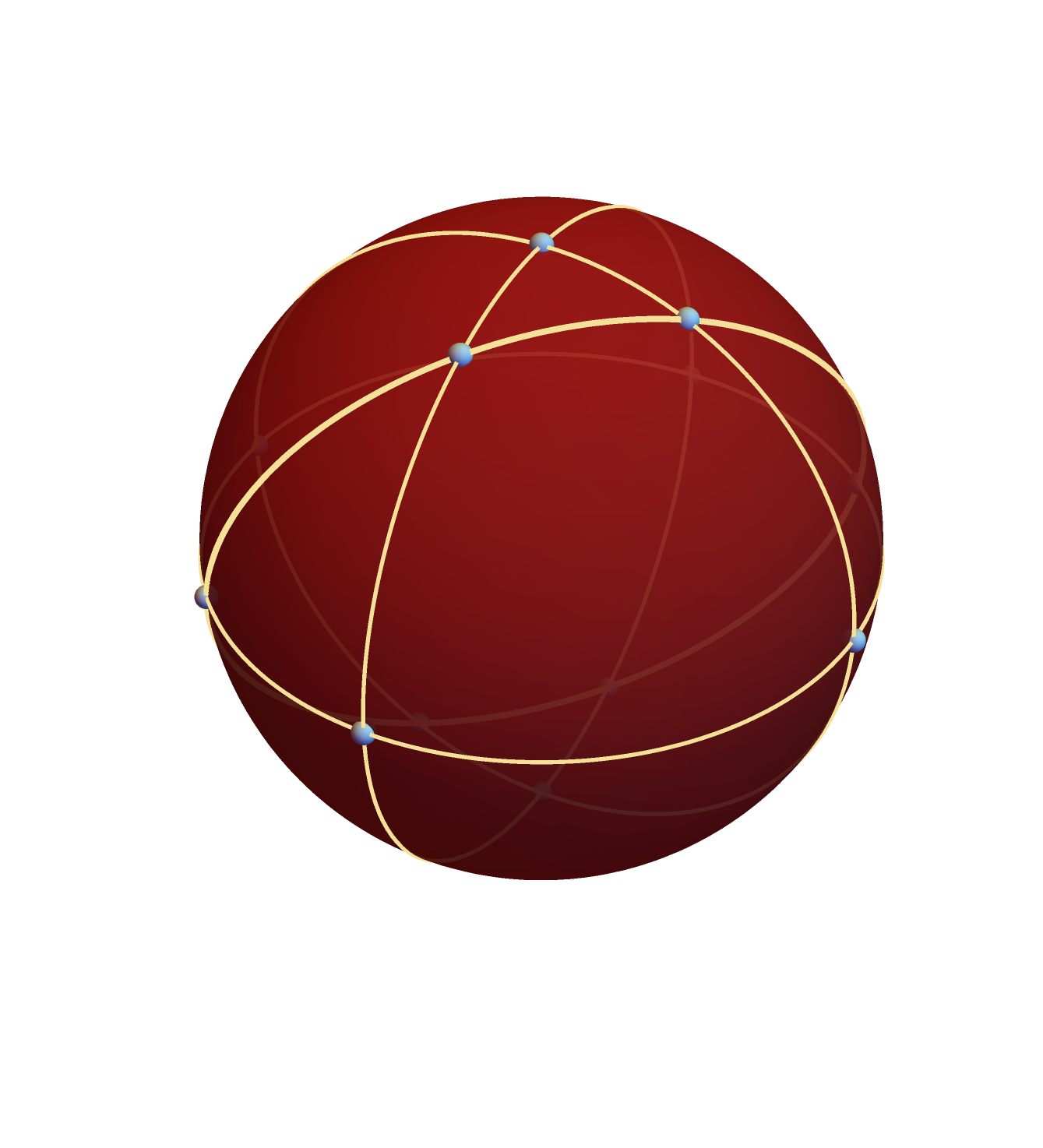
(a) Sunrise diagram

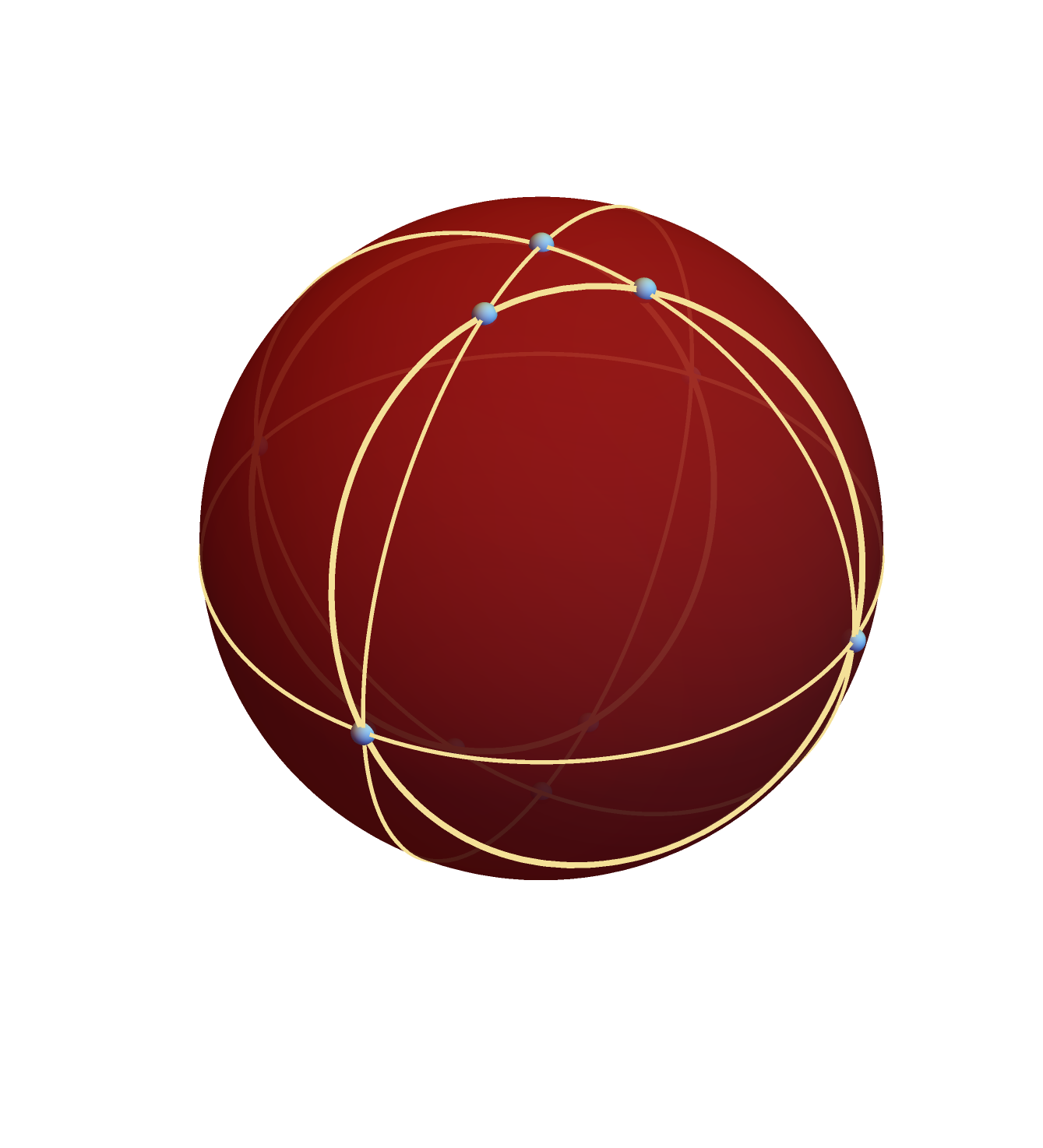
(b) Planar box diagram

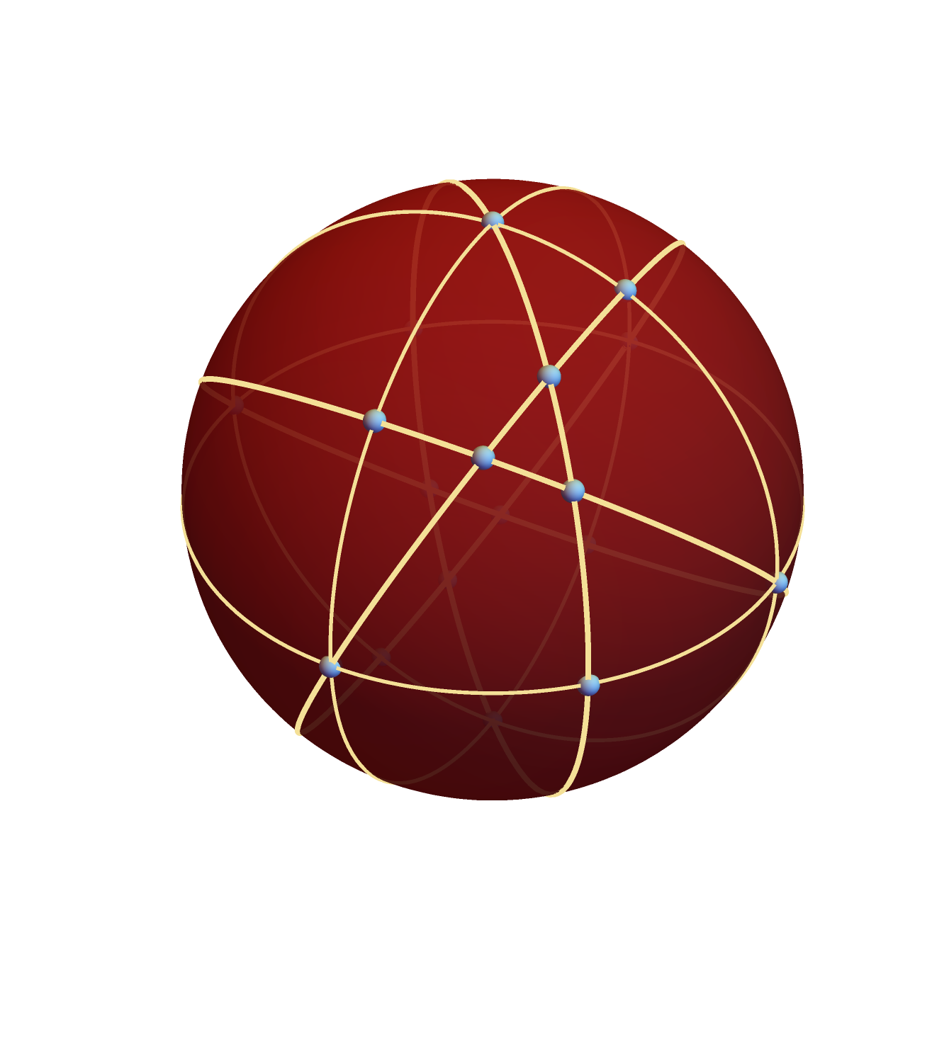
(c) ${}_{3}F_{2}$

Figure 1: Singular hypersurfaces $\mathcal{S}_{i}$ of the massless sunrise twist (42) on the left, massless 2-loop planar box twist (52) in the middle, and the ${}_{3}F_{2}$ twist (60) on the right. The red sphere (with identified antipodal points) depicts the real slice of the projective plane $\mathbb{C}\mathrm{P}^{2}$, whose equator is the line at infinity. The blue dots represent the intersection points collected in eqs. (43, 54, 61).

Example 1.

Consider the intersection $\langle\varphi_{L}\>|\>\varphi_{R}\rangle$ between:

$$\hat{\varphi}_{L}=\frac{1}{z_{1}^{2}z_{2}}\ ,\qquad\hat{\varphi}_{R}=\frac{1}{z_{1}^{2}z_{2}}\ .$$ (45)

Out of the six points collected in eq. (43) only two give non-trivial residues, yielding:

$$\langle\varphi_{L}\>|\>\varphi_{R}\rangle={\rm Res}_{z=(0,0)}(\psi\,\varphi_{R})+{\rm Res}_{z=(0,s)}(\psi\,\varphi_{R})=-\frac{1}{s^{2}}\frac{\gamma_{3}(\gamma_{1}+\gamma_{3})}{\gamma_{1}(1-\gamma_{1}^{2})\gamma_{2}}-\frac{1}{s^{2}}\frac{\gamma_{3}}{\gamma_{1}(1-\gamma_{1}^{2})}\ .$$ (46)

Example 2.

We can also compute $\langle\varphi_{L}\>|\>\varphi_{R}\rangle$ of meromorphic forms containing the $\mathcal{B}_{3}$ factor:

$$\hat{\varphi}_{L}=\frac{1}{z_{1}z_{2}(z_{1}+z_{2}-s)}\ ,\qquad\hat{\varphi}_{R}=\frac{1}{z_{1}z_{2}(z_{1}+z_{2}-s)^{2}}\ .$$ (47)

Out of the six points shown in eq. (43) the three points from the $U_{z}$ chart give non-zero residues:

$${\rm Res}_{z=(0,0)}(\psi\,\varphi_{R}) =-\tfrac{1}{s^{3}}\tfrac{1}{\gamma_{1}\gamma_{2}}\ ,$$ (48)

$${\rm Res}_{z=(s,0)}(\psi\,\varphi_{R}) =0-\tfrac{1}{s^{3}}\tfrac{1+\gamma_{1}+2\gamma_{2}+2\gamma_{3}}{\gamma_{2}(\gamma_{2}+\gamma_{3})(1+\gamma_{2}+\gamma_{3})}-\tfrac{1}{s^{3}}\Bigl{(}\tfrac{1-\gamma_{1}}{(1+\gamma_{3})(1+\gamma_{2}+\gamma_{3})}+\tfrac{1+\gamma_{1}}{\gamma_{3}(\gamma_{2}+\gamma_{3})}\Bigr{)}\ ,$$ (49)

$${\rm Res}_{z=(0,s)}(\psi\,\varphi_{R}) =-\tfrac{1}{s^{3}}\tfrac{1+2\gamma_{1}+\gamma_{2}+2\gamma_{3}}{\gamma_{1}(\gamma_{1}+\gamma_{3})(1+\gamma_{1}+\gamma_{3})}+0-\tfrac{1}{s^{3}}\tfrac{(1+\gamma_{1}+2\gamma_{3})(1+2\gamma_{1}+\gamma_{2}+2\gamma_{3})}{\gamma_{3}(1+\gamma_{3})(\gamma_{1}+\gamma_{3})(1+\gamma_{1}+\gamma_{3})}\ ,$$ (50)

where we separated contributions of the transformations shown in Table 1 into individual terms. By adding them up, the intersection number becomes:

$$\langle\varphi_{L}\>|\>\varphi_{R}\rangle ={\rm Res}_{z=(0,0)}(\psi\,\varphi_{R})+{\rm Res}_{z=(s,0)}(\psi\,\varphi_{R})+{\rm Res}_{z=(0,s)}(\psi\,\varphi_{R})$$

$$=-\frac{1}{s^{3}}\frac{(\gamma_{1}+\gamma_{2}+\gamma_{3})(1+\gamma_{1}+\gamma_{2}+\gamma_{3})}{\gamma_{1}\gamma_{2}\gamma_{3}(1+\gamma_{3})}\ .$$ (51)

3.2 Two-loop planar box diagram

Now we turn to the massless 2-loop planar box on the maximal cut in the Baikov representation with the twist:

$$u=\begin{cases}z_{1}^{\gamma_{1}}z_{2}^{\gamma_{2}}\>(st+s(z_{1}+z_{2})+z_{1}z_{2})^{\gamma_{3}}&\text{in $U_{z}$}\ ,\\ x_{1}^{\gamma_{1}}x_{2}^{-\gamma_{0}-\gamma_{3}}\,\bigl{(}x_{1}+sx_{2}+sx_{1}x_{2}+stx_{2}^{2}\bigr{)}^{\gamma_{3}}&\text{in $U_{x}$}\ ,\\ y_{1}^{-\gamma_{0}-\gamma_{3}}y_{2}^{\gamma_{2}}\,\bigl{(}sy_{1}+y_{2}+sy_{1}y_{2}+sty_{1}^{2}\bigr{)}^{\gamma_{3}}&\text{in $U_{y}$}\ ,\end{cases}$$ (52)

where $\gamma_{0}:=\gamma_{1}+\gamma_{2}+\gamma_{3}$, and the factors (9) are:

$$\{\mathcal{B}_{1},\mathcal{B}_{2},\mathcal{B}_{3}\}:=\{z_{1},z_{2},st+s(z_{1}+z_{2})+z_{1}\}\ .$$ (53)

There are $3+1+1=5$ intersection points in $\mathbb{C}\mathrm{P}^{2}$ of the singular hypersurfaces $\mathcal{S}_{i}$ (see Figure 1b), their location is as follows:

$$\mathbb{P}_{\omega}=\begin{cases}(z_{1},z_{2})\in\bigl{\{}(0,0),(-t,0),(0,-t)\bigr{\}}&\text{in $U_{z}$}\ ,\\ (x_{1},x_{2})=(0,0)&\text{in $U_{x}$}\ ,\\ (y_{1},y_{2})=(0,0)&\text{in $U_{y}$}\ .\end{cases}$$ (54)

Here we only consider intersection numbers between monomial $\varphi_{L}^{(\mathbf{2})}$ and $\varphi_{R}^{(\mathbf{2})}$ cocycles:

$$\varphi^{(\mathbf{2})}_{\mathchoice{\mathbin{\vbox{\hbox{\scalebox{1.0}{$\displaystyle\bullet$}}}}}{\mathbin{\vbox{\hbox{\scalebox{1.0}{$\textstyle\bullet$}}}}}{\mathbin{\vbox{\hbox{\scalebox{1.0}{$\scriptstyle\bullet$}}}}}{\mathbin{\vbox{\hbox{\scalebox{1.0}{$\scriptscriptstyle\bullet$}}}}}}=z_{1}^{n_{1}}z_{2}^{n_{2}}\>\mathrm{d}z_{1}\wedge\mathrm{d}z_{2}\ ,$$ (55)

with the same notation as in eq. (44).

Some of the intersection points (54) turn out to be degenerate: they have three singular hypersurfaces $\mathcal{S}_{i}$ passing through them. An example of this is the point $x=(0,0)$ located on the line at infinity, as can be seen from eq. (52) and Figure 1b. One way to amend this issue is to employ the resolution of singularities procedure (closely related to the sector decomposition algorithm, see Borowka:2017idc ; Heinrich:2021dbf ; Bogner:2007cr ). In Appendix B.3 we give further details and collect the full list of coordinate transformations used for computation of intersection numbers in this setup.

Example 3.

Let us consider the intersection number $\langle\varphi_{L}\>|\>\varphi_{R}\rangle$ between the two logarithmic forms:

$$\hat{\varphi}_{L}=\frac{1}{z_{1}z_{2}}\ ,\qquad\hat{\varphi}_{R}=\frac{1}{z_{1}z_{2}}\ .$$ (56)

Only the origins of the three charts (54) contribute to this intersection number producing:

$$\langle\varphi_{L}\>|\>\varphi_{R}\rangle ={\rm Res}_{z=(0,0)}(\psi\,\varphi_{R})+{\rm Res}_{x=(0,0)}(\psi\,\varphi_{R})+{\rm Res}_{y=(0,0)}(\psi\,\varphi_{R})$$

$$=\tfrac{1}{\gamma_{1}\gamma_{2}}+\Bigl{(}\tfrac{-1}{\gamma_{1}(\gamma_{2}+\gamma_{3})}+\tfrac{1}{(\gamma_{2}+\gamma_{3})(\gamma_{0}+\gamma_{3})}\Bigr{)}+\Bigl{(}\tfrac{1}{(\gamma_{1}+\gamma_{3})(\gamma_{0}+\gamma_{3})}+\tfrac{-1}{\gamma_{2}(\gamma_{1}+\gamma_{3})}\Bigr{)}\ .$$ (57)

Example 4.

Similar to Example 1, we compute the intersection between:

$$\hat{\varphi}_{L}=\frac{1}{z_{1}^{2}z_{2}}\ ,\qquad\hat{\varphi}_{R}=\frac{1}{z_{1}^{2}z_{2}}\ .$$ (58)

We find the three points from $\mathbb{P}_{\omega}$ contribute to this intersection number, resulting in:

$$\langle\varphi_{L}\>|\>\varphi_{R}\rangle ={\rm Res}_{z=(0,0)}(\psi\,\varphi_{R})+{\rm Res}_{z=(0,-t)}(\psi\,\varphi_{R})+{\rm Res}_{x=(0,0)}(\psi\,\varphi_{R})$$

$$=-\tfrac{1}{t^{2}}\tfrac{\gamma_{3}(\gamma_{1}+\gamma_{3})}{\gamma_{1}\gamma_{2}(1-\gamma_{1}^{2})}-\tfrac{1}{s^{2}t^{2}}\tfrac{\gamma_{3}(s-t)^{2}}{\gamma_{1}(1-\gamma_{1}^{2})}+\tfrac{1}{s^{2}}\tfrac{\gamma_{3}(\gamma_{1}+\gamma_{3})}{\gamma_{1}(1-\gamma_{1}^{2})(\gamma_{2}+\gamma_{3})}\ .$$ (59)

Chart	Point	Coordinate transformation(s)
$U_{z}$	$(0,0)$	$\bigl{\{}(z_{1}z_{2},\>z_{2}),(z_{1},\>z_{1}z_{2}),((1+z_{1})z_{2},\>z_{2})\bigr{\}}$
	$(0,s)$	$(z_{1},\>s+z_{2})$
	$(s,s)$	$\bigl{\{}(s+z_{1}z_{2},\>s+z_{2}),(s+z_{1},\>s+z_{1}z_{2}),(s+(1+z_{1})z_{2},\>s+z_{2})\bigr{\}}$
	$(1,0)$	$(1+z_{1},\>z_{2})$
	$(1,s)$	$(1+z_{1},\>s+z_{2})$
	$(1,1)$	$\bigl{\{}(1+z_{1}z_{2},\>1+z_{2}),(1+z_{1},\>1+z_{1}z_{2}),(1+(1+z_{1})z_{2},\>1+z_{2})\bigr{\}}$
$U_{x}$	$(0,0)$	$\bigl{\{}(z_{1},\>\tfrac{1}{z_{2}}),(\tfrac{1}{z_{2}},\>\tfrac{1}{z_{1}z_{2}}),(1+z_{1},\>\tfrac{1}{z_{2}})\bigr{\}}$
	$(1,0)$	$(\tfrac{1+z_{1}}{z_{2}},\>\tfrac{1}{z_{2}})$
$U_{y}$	$(0,0)$	$\bigl{\{}(\tfrac{1}{z_{1}z_{2}},\>\tfrac{1}{z_{1}}),(\tfrac{1}{z_{1}},\>z_{2}),(\tfrac{1}{(s^{-1}+z_{1})z_{2}},\tfrac{1}{s^{-1}+z_{1}})\bigr{\}}$

Table 2: Intersection points $\mathbb{P}_{\omega}$ (middle) from the three coordinate charts of $\mathbb{C}\mathrm{P}^{2}$ (left) that contribute to the intersection numbers between forms (62) with the ${}_{3}F_{2}$ twist (60). On the right we show the coordinate transformations used to compute the residues (20). We sum over all the contributions of each displayed transformation.

3.3 ${}_{3}F_{2}$ hypergeometric function

Another setup with degenerate intersection points is the ${}_{3}F_{2}$ hypergeometric function, whose twist looks like this:

$$u=\begin{cases}z_{1}^{\gamma_{1}}z_{2}^{\gamma_{2}}\>(1-z_{1})^{\gamma_{3}}\>(s-z_{2})^{\gamma_{4}}\>(z_{1}-z_{2})^{\gamma_{5}}&\text{in $U_{z}$}\ ,\\ (-1)^{\gamma_{3}+\gamma_{5}}\>x_{1}^{\gamma_{1}}x_{2}^{-\gamma_{0}}\>(x_{1}-x_{2})^{\gamma_{3}}\>(sx_{2}-1)^{\gamma_{4}}\>(1-x_{1})^{\gamma_{5}}&\text{in $U_{x}$}\ ,\\ (-1)^{\gamma_{3}}\>y_{1}^{-\gamma_{0}}y_{2}^{\gamma_{2}}\>(1-y_{1})^{\gamma_{3}}\>(sy_{1}-y_{2})^{\gamma_{4}}\>(1-y_{2})^{\gamma_{5}}&\text{in $U_{y}$}\ ,\end{cases}$$ (60)

where $\gamma_{0}:=\gamma_{1}+\ldots+\gamma_{5}$ . The five singular hypersurfaces $\mathcal{S}_{i}$ intersect at the following $6+2+1=9$ points (see Figure 1c):

$$\mathbb{P}_{\omega}=\begin{cases}(z_{1},z_{2})\in\bigl{\{}(0,0),(0,s),(s,s),(1,0),(1,s),(1,1)\bigr{\}}&\text{in $U_{z}$}\ ,\\ (x_{1},x_{2})\in\bigl{\{}(0,0),(1,0)\bigr{\}}&\text{in $U_{x}$}\ ,\\ (y_{1},y_{2})=(0,0)&\text{in $U_{y}$}\ .\end{cases}$$ (61)

We compute intersection numbers between generic $\varphi_{L}^{(\mathbf{2})}$ and $\varphi_{R}^{(\mathbf{2})}$ cocyles:

$$\varphi^{(\mathbf{2})}_{\mathchoice{\mathbin{\vbox{\hbox{\scalebox{1.0}{$\displaystyle\bullet$}}}}}{\mathbin{\vbox{\hbox{\scalebox{1.0}{$\textstyle\bullet$}}}}}{\mathbin{\vbox{\hbox{\scalebox{1.0}{$\scriptstyle\bullet$}}}}}{\mathbin{\vbox{\hbox{\scalebox{1.0}{$\scriptscriptstyle\bullet$}}}}}}=z_{1}^{n_{1}}z_{2}^{n_{2}}\>(1-z_{1})^{n_{3}}(s-z_{2})^{n_{4}}(z_{1}-z_{2})^{n_{5}}\>\mathrm{d}z_{1}\wedge\mathrm{d}z_{2}\ ,$$ (62)

with the same notation as in eq. (44).

Example 5.

In continuation of Example 3 we calculate the intersection of the logarithmic forms:

$$\hat{\varphi}_{L}=\frac{1}{z_{1}z_{2}}\ ,\qquad\hat{\varphi}_{R}=\frac{1}{z_{1}z_{2}}\ .$$ (63)

Once again, only the origins of the charts contribute to this intersection number giving the total:

$$\langle\varphi_{L}\>|\>\varphi_{R}\rangle ={\rm Res}_{z=(0,0)}(\psi\,\varphi_{R})+{\rm Res}_{x=(0,0)}(\psi\,\varphi_{R})+{\rm Res}_{y=(0,0)}(\psi\,\varphi_{R})$$

$$=\Bigl{(}\tfrac{1}{\gamma_{1}(\gamma_{1}+\gamma_{2}+\gamma_{5})}+\tfrac{1}{\gamma_{2}(\gamma_{1}+\gamma_{2}+\gamma_{5})}+0\Bigr{)}$$ (64)

$$\quad+\Bigl{(}\tfrac{-1}{\gamma_{1}(\gamma_{2}+\gamma_{4}+\gamma_{5})}+\tfrac{1}{\gamma_{0}(\gamma_{2}+\gamma_{4}+\gamma_{5})}+0\Bigr{)}+\Bigl{(}\tfrac{1}{\gamma_{0}(\gamma_{1}+\gamma_{3}+\gamma_{5})}+\tfrac{-1}{\gamma_{2}(\gamma_{1}+\gamma_{3}+\gamma_{5})}+0\Bigr{)}\ .$$

This concludes our collection of examples, for intersection numbers in $n=2$ variables, involving Feynman integrals and other mathematical functions. Let us remark, that the presented method is also applicable to meromorphic $n$-forms in higher dimensions.

4 Algebraic solutions

In this section, we will introduce an algebraic solution for the contribution to the intersection number coming from each individual residue. The main formula of this section, eq. (72), is derived by solving the $n$PDE using an ansatz. We will start the section by introducing an essential combinatorial object, that of vector compositions.

4.1 Vector Compositions

Vector compositions are a convenient tool for manipulating algebraic expressions involving multivariate monomials, in particular when dealing with product of multivariate series.

Definition 1.

Vector compositions

$$S=\text{VC}(\boldsymbol{\tau})\qquad\text{with}\qquad\boldsymbol{\tau}=(\tau_{1},\ldots,\tau_{n})$$ (65)

are a function of $n$ non-negative integers $\tau_{1}$ to $\tau_{n}$. Its output $S$ is a set of ordered lists $\sigma$, each containing a number of $n$-vectors $\boldsymbol{s}$, with the property $\sum_{\boldsymbol{s}\in\sigma}\boldsymbol{s}=\boldsymbol{\tau}$ ($\boldsymbol{s}$ vectors contain non-negative integers; the zero-vector is excluded, corresponding to all $\boldsymbol{s}>\boldsymbol{0}$). Each $\boldsymbol{s}$ can be represented as a step in $\mathbb{Z}^{n}$, therefore $\sigma$, being a collection of steps, can be mapped to a path in $\mathbb{Z}^{n}$, going from $\boldsymbol{0}$ to $\boldsymbol{\tau}$. Within this representation, $S$ can be viewed as the set of all paths $\mathbb{Z}^{n}$, connecting $\boldsymbol{0}$ to $\boldsymbol{\tau}$, in one or in multiple (ordered) steps, counted by the size of $\sigma$, namely having $|\sigma|=1,2,\ldots$ m, with $m:=\sum_{i=1}^{n}\tau_{i}\,.$

Example 6 ($n=1$ case).

In the univariate case, the vector $\boldsymbol{\tau}$ has just one entry, say $\boldsymbol{\tau}=(m)$ with $m\in{\mathbb{N}}$, therefore the vector compositions reduce to standard compositions, i.e. $\text{VC}(\boldsymbol{\tau})=\text{comp}(m)$. Compositions are a known operation from combinatorics which describe the number of (ordered) ways an integer can be expressed as a sum of positive integers. For illustration, let us choose $\boldsymbol{\tau}=(4)$

$${\rm VC}(\boldsymbol{\tau})=\text{comp}(4)=\big{\{}(4),(3,1),(2,2),(1,3),(2,1,1),(1,2,1),(1,1,2),(1,1,1,1)\big{\}}$$ (66)

Example 7 ($n=2$ case).

The two dimensional case, where the vector $\boldsymbol{\tau}$ has two components, is the first non-trivial case for applying vector composition. For illustration, let us consider $\boldsymbol{\tau}=(1,2)$, yielding

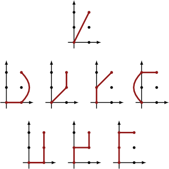
Figure 2: Paths appearing in eq. (67).

$$\text{VC}(\boldsymbol{\tau})=\Big{\{} \left(\tbinom{1}{2}\right),$$

$$\left(\tbinom{1}{0},\tbinom{0}{2}\right),\left(\tbinom{1}{1},\tbinom{0}{1}\right),\left(\tbinom{0}{1},\tbinom{1}{1}\right),\left(\tbinom{0}{2},\tbinom{1}{0}\right),$$ (67)

$$\left(\tbinom{1}{0},\tbinom{0}{1},\tbinom{0}{1}\right),\left(\tbinom{0}{1},\tbinom{1}{0},\tbinom{0}{1}\right),\left(\tbinom{0}{1},\tbinom{0}{1},\tbinom{1}{0}\right)\Big{\}}$$

where the three rows correspond to entries with $|\sigma|$ being 1, 2, and 3, respectively. Each element of $\text{VC}(\boldsymbol{\tau})$ admits a representation in terms of lattice paths in $\mathbb{Z}^{2}$, as shown in Figure 2.

More details on vector compositions can be found in e.g. andrews_1984 . In the current context, they turn out to be a useful tool to express the solution of the $n$PDE eq. (38).

4.2 Algebraic expression for residues

In Section 2 we saw that multivariate intersection numbers can be expressed as a sum over contributions from a number of points, with each contribution expressed as a residue. In the “right rescaling” framework of Section 2.5 the relation is given as

$$\langle\varphi_{L}\>|\>\varphi_{R}\rangle=\sum_{p\in\mathbb{P}_{\omega}}\text{Res}_{z=p}(f)$$ (68)

where $f$ is defined as the solution of eq. (38), namely

$${\hat{\nabla}}_{\omega_{R,1}}\cdots{\hat{\nabla}}_{\omega_{R,n}}\,f={\hat{\phi}}\ ,\qquad{\rm with}\;\qquad{\hat{\phi}}=\hat{\varphi}_{L}\hat{\varphi}_{R}\ ,$$ (69)

and where

$${\hat{\nabla}}_{\omega_{R,i}}:=(\partial_{z_{i}}+(\partial_{z_{i}}w))\ ,\qquad\text{with}\;\qquad w:=\log(u/\hat{\varphi}_{R})\ .$$ (70)

In Section 2.4 it was discussed how to solve systems of the form of eq. (69) by making a series ansatz for $f$ and solving it locally around each point, in what is essentially an analytic use of the “Frobenius method”. In this section we are going to pursue that direction a step further, to obtain an algebraic solution for each term in eq. (68). The first step is to write $w$ and $\hat{\phi}$ as series around each point, where the appropriate variable changes have been made in order to ensure that the point is located at $\boldsymbol{z}=\boldsymbol{0}$ and in addition that the series expansions are well defined so no further variable changes (or blowups) are needed. With this we may write

$${\hat{\phi}} =\sum_{\boldsymbol{i}=\boldsymbol{\mu}_{\boldsymbol{\phi}}\!\!\!}^{\boldsymbol{\infty}}\phi_{\boldsymbol{i}}z^{\boldsymbol{i}}\qquad\quad\text{and}\qquad\quad w=\log(u/\hat{\varphi}_{R})=\sum_{\boldsymbol{i}=\boldsymbol{0}}^{\boldsymbol{\infty}}w_{\boldsymbol{i}}z^{\boldsymbol{i}}\;+\;\sum_{j=1}^{n}v_{j}\log(z_{j})$$ (71)

where $z^{\boldsymbol{i}}:=z_{1}^{i_{1}}\cdots z_{n}^{i_{n}}$. In this notation $\boldsymbol{\mu}_{\boldsymbol{\phi}}$ should be interpreted as the powers corresponding to the leading term in the expansion of $\hat{\varphi}_{L}\hat{\varphi}_{R}$. The $w$-expansion begins at powers $\boldsymbol{0}$ (lower ones cannot appear when $u$ is of the form $\prod_{i}\mathcal{B}_{i}^{\gamma_{i}}$, as in our case). Using an ansatz for $f$ as a Laurent series expansion around each intersection point, the $n$PDE constraints the coefficients, so that the residue of $f$ can be obtained in closed form as,

$$\boxed{\,\text{Res}(f)\,=\!\sum_{\boldsymbol{\tau}=\boldsymbol{0}}^{\!{-}\boldsymbol{\mu}_{\boldsymbol{\phi}}{-}\boldsymbol{2}}\!\sum_{\sigma\in\text{VC}(\boldsymbol{\tau})}\!\left(\frac{(-1)^{|\sigma|}}{U(\boldsymbol{0},\boldsymbol{0})}\prod_{i=1}^{|\sigma|}\frac{U(\boldsymbol{\sigma}_{\boldsymbol{i}},\boldsymbol{\mathcal{T}}_{\!\boldsymbol{i}})}{U(\boldsymbol{0},\boldsymbol{\mathcal{T}}_{\!\boldsymbol{i}})}\right)\!\phi_{-\boldsymbol{\tau}-\boldsymbol{2}}\,}$$ (72)

where

$$\boldsymbol{\mathcal{T}}_{\!\boldsymbol{i}}:=\boldsymbol{\tau}-\sum_{j<i}\!\boldsymbol{\sigma}_{\boldsymbol{j}}$$ (73)

and $U$ is a function dependent only on the terms in the expansion of $w$, which is conveniently defined in terms of an auxiliary function, $R$, as

$$U(\boldsymbol{\lambda},\boldsymbol{\eta}) :=R(\boldsymbol{\lambda},\,{-}\boldsymbol{\eta}{-}\boldsymbol{1})$$ (74)

whose general definition is reported in Appendix C.1.2. Here, for illustration purposes, we showcase its expressions for a few small values of $n$:

$$\bullet\ n=1:\quad R(\alpha,\beta)\,=\,(\beta{+}v)\delta_{\alpha,0}+\alpha w_{\alpha}$$ (75)

$$\bullet\ n=2: R(\boldsymbol{\alpha},\boldsymbol{\beta})=(\beta_{1}{+}v_{1})(\beta_{2}{+}v_{2})\delta_{\boldsymbol{\alpha},\boldsymbol{0}}+\big{(}\alpha_{1}\alpha_{2}+\alpha_{1}(\beta_{2}{+}v_{2})+\alpha_{2}(\beta_{1}{+}v_{1})\big{)}w_{\boldsymbol{\alpha}}$$

$$\>+\sum_{\boldsymbol{j}\,=\,\boldsymbol{0}}^{\boldsymbol{\alpha}}(\alpha_{1}{-}j_{1})j_{2}\,w_{\boldsymbol{\alpha}-\boldsymbol{j}}w_{\boldsymbol{j}}$$ (76)

$$\bullet\ n=3:\quad R(\boldsymbol{\alpha},\boldsymbol{\beta})=(\beta_{1}{+}v_{1})(\beta_{2}{+}v_{2})(\beta_{3}{+}v_{3})\delta_{\boldsymbol{\alpha},\boldsymbol{0}}$$

$$\>+\big{(}(\alpha_{1}{+}\beta_{1}{+}v_{1})(\alpha_{2}{+}\beta_{2}{+}v_{2})(\alpha_{3}{+}\beta_{3}{+}v_{3})-(\beta_{1}{+}v_{1})(\beta_{2}{+}v_{2})(\beta_{3}{+}v_{3})\big{)}w_{\boldsymbol{\alpha}}$$

$$\>+\sum_{\boldsymbol{j}\,=\,\boldsymbol{0}}^{\boldsymbol{\alpha}}\big{(}(\alpha_{1}{-}j_{1})j_{2}(j_{3}{+}\beta_{3}{+}v_{3})+(\alpha_{2}{-}j_{2})j_{3}(j_{1}{+}\beta_{1}{+}v_{1})+(\alpha_{3}{-}j_{3})j_{1}(j_{2}{+}\beta_{2}{+}v_{2})\big{)}w_{\boldsymbol{\alpha}{-}\boldsymbol{j}}w_{\boldsymbol{j}}$$

$$\>+\sum_{\boldsymbol{j}=\boldsymbol{0}}^{\boldsymbol{\alpha}}\,\sum_{\boldsymbol{l}=\boldsymbol{0}}^{\boldsymbol{\alpha}{-}\boldsymbol{j}}\,(\alpha_{1}{-}j_{1}{-}l_{1})\,j_{2}\,l_{3}\,w_{\boldsymbol{\alpha}{-}\boldsymbol{j}{-}\boldsymbol{l}}\,w_{\boldsymbol{j}}\,w_{\boldsymbol{l}}$$ (77)

For a general $n$-variate expression of $R$, see Appendix C.1.2.

The residue formula in eq. (72), using vector compositions, constitutes the third main result of this work. Further details on its derivation can be found in Appendix C.

The arXiv version of this paper is supplemented with a Mathematica implementation of eq. (72), consisting of a package algebraic_residue.m and a notebook file load_algebraic_residue.nb that contains examples of its use.

4.3 Example

Here we show an application of the algebraic formula eq. (72).

Example 8.

Using the setup of Section 3.1, let us compute $\langle\varphi_{L}\>|\>\varphi_{R}\rangle$ with

$$\hat{\varphi}_{L}=\frac{1}{z_{1}z_{2}}\,,\qquad\hat{\varphi}_{R}=\frac{1}{z_{1}z_{2}}\ .$$ (78)

In the “right rescaling” scheme, the first step is to compute $\Phi=\varphi_{L}\hat{\varphi}_{R}$ at each of the points in Table 1 and identify the leading term corresponding to the $\boldsymbol{\mu}_{\boldsymbol{\phi}}$-vector. The result is given in Table 3.

point	$\hat{\Phi}$	${-}\boldsymbol{\mu}_{\boldsymbol{\phi}}{-}\boldsymbol{2}$
1	$z_{1}^{-2}z_{2}^{-2}$	$\{0,0\}$
2a	$(s{+}z_{1}z_{2})^{-2}$	$\{-2,-2\}$
2b	$(s{+}z_{1})^{-2}z_{2}^{-2}$	$\{-2,0\}$
2c	$(s{+}z_{2}(z_{1}{-}1))^{-2}\!$	$\{-2,-2\}$
3a	$z_{1}^{-2}(s{+}z_{2})^{-2}$	$\{0,-2\}$
3b	$(s{+}z_{1}z_{2})^{-2}$	$\{-2,-2\}$

   point $\hat{\Phi}$ ${-}\boldsymbol{\mu}_{\boldsymbol{\phi}}{-}\boldsymbol{2}$ 3c $(z_{1}{-}1)^{-2}(z_{2}{+}s)^{-2}$ $\{-2,-2\}$ 4 $z_{1}^{-2}z_{2}^{-2}$ $\{0,0\}$ 5a $(z_{1}z_{2}{-}1)^{-2}$ $\{-2,-2\}$ 5b $(z_{1}{-}1)^{-2}z_{2}^{-2}$ $\{-2,0\}$ 5c $((s{+}z_{1})z_{2}{-}1)^{-2}$ $\{-2,-2\}$ 6 $z_{1}^{-2}z_{2}^{-2}$ $\{0,0\}$

Table 3: Values for $\hat{\Phi}$ and $\boldsymbol{\mu}_{\boldsymbol{\phi}}$ at the twelve sub-intersection points for Example 8. The points are defined in Table 1, and the additional labels (a,b,c) refer to the adopted coordinate transformation.

We see from the general expression (72) that a given point will only contribute if $-\boldsymbol{\mu}_{\boldsymbol{\phi}}-\boldsymbol{2}\geq\boldsymbol{0}$. So we realize that there only will be contributions from three of the intersection points: 1, 4, and 6. In each case eq. (72) will contain one term only, of the form

$$\text{Res}(f)=\frac{\phi_{-2,-2}}{(v_{1}{-}1)(v_{2}{-}1)}\ .$$ (79)

We observe that $\phi_{-2,-2}=1$ at each of the three points, while the values of the $v_{i}$ depend on the considered point, and are computed locally. The non-vanishing expressions of $\text{Res}(f)$, are:

$$\text{Point 1}:\frac{1}{\gamma_{1}\gamma_{2}}\qquad\text{Point 4}:\frac{-1}{\gamma_{1}(\gamma_{1}{+}\gamma_{2}{+}\gamma_{3})}\qquad\text{Point 6}:\frac{-1}{\gamma_{2}(\gamma_{1}{+}\gamma_{2}{+}\gamma_{3})}\ ,$$ (80)

therefore, the intersection number is obtained by adding them up, as:

$$\langle\varphi_{R}\>|\>\varphi_{L}\rangle =\frac{\gamma_{3}}{\gamma_{1}\gamma_{2}(\gamma_{1}{+}\gamma_{2}{+}\gamma_{3})}\ ,$$ (81)

which is the correct expected results.

5 Conclusion

In this work we proposed a new computational method for the evaluation of intersection numbers for twisted meromorphic $n$-forms through Stokes’ theorem, which is based on the solution of a $n$-th order partial differential equation ($n$PDE). Our finding can be summarised simply as:

$$\langle\varphi_{L}\>|\>\varphi_{R}\rangle=\frac{1}{(2\pi i)^{n}}\int(u\,\varphi_{L,c})\wedge(u^{-1}\,\varphi_{R})=\frac{1}{(2\pi i)^{n}}\oint(u^{-1}\,\varphi_{R})\int(u\,\varphi_{L})\ .$$ (82)

The evaluation of the last integral is performed by multivariate Laurent series expansions and multivariate residues. The analytic properties of the intersection numbers and of the $n$PDE yielded the algebraic determination of the contributing residues, which we were able to cast in closed forms for an efficient evaluation.

The presented method requires the knowledge of the intersection points as input. In the case of a twist corresponding to a hyperplane arrangement and normal crossing at the intersection points, this information can be easily extracted from the integrand. Instead, for generic configurations, when more hypersurfaces pass through a given intersection point, the desingularization procedure constitutes a challenging, hence interesting, mathematical problem.

The formulation of the intersection number for twisted cohomology presented here applies to the case of regulated singularities. We are confident that it can be extended to the relative cohomology case, where the singularities of the integral are not regulated within the twist.

The new method presented here can be applied to derive linear relations, differential equations, difference equations, and quadratic relations for Feynman integrals as well as for a wider class of functions, such as Aomoto-Gel’fand integrals, Euler-Mellin integrals, and GKZ hypergeometric functions. Therefore the method can be useful for computational (quantum) field theory, and computational differential and algebraic topology.

Acknowledgements

We wish to acknowledge interesting and stimulating discussions on intersection theory with Sergio Cacciatori, Yoshiaki Goto, Saiei Matsubara-Heo, Keiji Matsumoto, and Nobuki Takayama, at various stages. We would like to thank Sebastian Mizera for discussions and comments on the manuscript, and Henrik Munch for many good discussions and various checks. H.F. would like to thank Cristian Vergu for stimulating discussions.
We also would like to acknowledge the anonymous referee for her/his suggestions about improving our manuscripts.

V.C. is supported by the Diagrammalgebra Stars Wild-Card Grant UNIPD. H.F. is partially supported by a Carlsberg Foundation Reintegration Fellowship, and has received funding from the European Union’s Horizon 2020 research and innovation program under the Marie Skłodowska-Curie grant agreement No. 847523 ‘INTERACTIONS’. The work of M.K.M. is supported by Fellini - Fellowship for Innovation at INFN funded by the European Union’s Horizon 2020 research and innovation programme under the Marie Skłodowska-Curie grant agreement No 754496. F.G. is supported by Fondazione Cassa di Risparmio di Padova e Rovigo (CARIPARO).

Appendix A Relation to Matsumoto’s algorithm

In this appendix we adopt the notation of matsumoto1998 (see also Mizera:2019gea for a review) and explicitly derive the $n$PDE (31) in the $n=2$ variable setting.

Let us consider an intersection number among two holomorphic $2$-forms $\varphi_{L}$ and $\varphi_{R}$, and assume that any two hypersurfaces $\mathcal{S}_{i}$ and $\mathcal{S}_{j}$ defined in eq. (1) intersect at point(s), such that no other $\mathcal{S}_{k}$ with $k\neq i,j$ passes through it. The main idea of matsumoto1998 is to find an explicit $2$-form $\varphi_{L,c}$ with compact support in the same cohomology class of $\varphi_{L}$ . This $2$-form appears in the definition of the intersection number integral (20):

$$\langle\varphi_{L}\>|\>\varphi_{R}\rangle=(2\pi\mathrm{i})^{-2}\,\int_{X}\varphi_{L,c}\wedge\varphi_{R}\ .$$ (83)

We associate an intersection point $p_{ij}:=\mathcal{S}_{i}\cap\mathcal{S}_{j}$ with each pair of indices $(i,j)$ with $i<j$. For a singular hypersurface $\mathcal{S}_{i}$ we introduce two tubular neighborhoods $V_{i}$ and $U_{i}$ around it of radius $\epsilon_{1}$ and $\epsilon_{2}$ respectively, with $\epsilon_{1}<\epsilon_{2}$ , such that $V_{i}\subset U_{i}$ . Following matsumoto1998 , we then write an explicit formula for the compactly supported $2$-form:

$$\varphi_{L,c}=\varphi_{L}-\nabla_{\omega}\left(\sum_{j}h_{j}\left(\>\sum_{i<j}\mathrm{d}h_{i}\>\psi_{p_{ij}}+\prod_{i<j}(1-h_{i})\>\psi^{j}_{p_{ij}}\right)\right)\ ,$$ (84)

where $h_{j}$ is a smoothened version of the Heaviside step function: $h_{j}=1$ in $V_{j}$ , $h_{j}=0$ outside $U_{j}$ , and it smoothly interpolates between the two boundary values $0\leq h_{j}\leq 1$ in $U_{j}\setminus V_{j}$ . These properties of $h_{j}$ imply that the two forms coincide $\varphi_{L,c}=\varphi_{L}$ outside of the singular neighborhood $\cup_{j}U_{j}\supset\cup_{j}\mathcal{S}_{j}$ .

Furthermore, it is not difficult to show that eq. (84) has compact support, i.e. the $2$-form $\varphi_{L,c}$ vanishes on the singular neighborhood $\cup_{j}V_{j}\subset\cup_{j}U_{j}$, if we impose certain constraints on the auxiliary $0$- and $1$-forms appearing on the RHS of eq. (84). For our purposes here it is enough to investigate these constraints locally around a given intersection point $p_{ij}$ for some fixed $i$ and $j$, where we introduce local coordinates $(z_{1},z_{2})$, such that the hypersurfaces $\mathcal{S}_{i}$ and $\mathcal{S}_{j}$ are parametrized by $z_{1}=0$ and $z_{2}=0$ respectively. Then the auxiliary 1-forms $\psi^{i}$ and $\psi^{j}$, and the 0-form $\psi$ (we will drop the subscripts in the following) from eq. (84) must satisfy the following differential equations matsumoto1998 :

$$\nabla_{\omega}\psi^{i} =\varphi_{L} \text{on $U_{i}:=\bigl{\{}(z_{1},z_{2})\>\big{|}\>|z_{1}|\leq\epsilon_{2}\bigr{\}}$}\ ,$$

$$\nabla_{\omega}\psi^{j} =\varphi_{L} \text{on $U_{j}:=\bigl{\{}(z_{1},z_{2})\>\big{|}\>|z_{2}|\leq\epsilon_{2}\bigr{\}}$}\ ,$$ (85)

$$\nabla_{\omega}\psi =\psi^{i}-\psi^{j}\qquad \text{on $U_{i}\cap U_{j}$}\ ,$$

with the $z$-dependence shown explicitly:

$$\psi^{i}=\hat{\psi}^{i}(z_{1},z_{2})\>\mathrm{d}z_{2}\ ,\qquad\psi^{j}=\hat{\psi}^{j}(z_{1},z_{2})\>\mathrm{d}z_{1}\ ,\qquad\psi\equiv\hat{\psi}(z_{1},z_{2})\ .$$ (86)

Then on the polydisc $U_{i}\cap U_{j}$ eq. (84) reduces to:

$$\varphi_{L,c}=(1-h_{j})(1-h_{i})\>\varphi_{L}-(1-h_{j})\>\mathrm{d}h_{i}\wedge\psi^{i}-(1-h_{i})\>\mathrm{d}h_{j}\wedge\psi^{j}+\psi\>\mathrm{d}h_{i}\wedge\mathrm{d}h_{j}\ ,$$ (87)

which vanishes on the inner polydisc $V_{i}\cap V_{j}$ . Similarly one can show that eq. (84) vanishes on the rest of the singular tube $V_{j}\setminus\cup_{i\neq j}U_{i}$ for each $j$, which proves that $\varphi_{L,c}$ indeed has compact support.

In the integral (83) the compactly supported $2$-form $\varphi_{L,c}$ is wedged against the holomorphic form $\varphi_{R}$, hence out of eq. (84) only the anti-holomorphic part will contribute to the intersection number. The only source of this is the last term in eq. (87), so that the intersection number integral localizes onto neighborhoods of intersection points $p_{ij}$ as:

$$\langle\varphi_{L}\>|\>\varphi_{R}\rangle=(2\pi\mathrm{i})^{-2}\sum_{p_{ij}}\int_{(U_{i}\setminus V_{i})\cap(U_{j}\setminus V_{j})}\psi\>\mathrm{d}h_{i}\wedge\mathrm{d}h_{j}\wedge\varphi_{R}\ ,$$ (88)

where the integration domain is a difference of two polydiscs:

$$(U_{i}\setminus V_{i})\cap(U_{j}\setminus V_{j})=\{(z_{1},z_{2})\,|\,\epsilon_{1}\leq|z_{1}|,|z_{2}|\leq\epsilon_{2}\}\equiv(U_{i}\cap U_{j})\setminus(V_{i}\cap V_{j})$$ (89)

Each integral in eq. (88) can be computed applying Stokes’ theorem one variable at time. Recalling that $h_{i}$ vanishes on $\partial U_{i}=\{z_{1}\,|\,|z_{1}|=\epsilon_{2}\}$ (and similar for $h_{j}$), we obtain the following:

$$\begin{split}(2\pi\mathrm{i})^{-2}\int_{\epsilon_{1}\leq|z_{1}|,|z_{2}|\leq\epsilon_{2}}\mathrm{d}h_{i}\wedge\mathrm{d}h_{j}\wedge\psi\,\varphi_{R}&=-(2\pi\mathrm{i})^{-2}\int_{|z_{1}|=\epsilon_{1},\epsilon_{1}\leq|z_{2}|\leq\epsilon_{2}}\mathrm{d}h_{j}\wedge\psi\varphi_{R}\\ &=-(2\pi\mathrm{i})^{-1}\int_{\epsilon_{1}\leq|z_{2}|\leq\epsilon_{2}}\mathrm{d}h_{j}\wedge\bigl{(}{\rm Res}_{z_{1}=0}\,\psi\varphi_{R}\bigr{)}\\ &=(2\pi\mathrm{i})^{-1}\int_{|z_{2}|=\epsilon_{1}}\,{\rm Res}_{z_{1}=0}\,\psi\varphi_{R}\\ &={\rm Res}_{z_{2}=0}\bigl{(}{\rm Res}_{z_{1}=0}\,\psi\varphi_{R}\bigr{)}\ .\end{split}$$ (90)

We would like to emphasise, that in ref. matsumoto1998 the 0-form $\psi$ is determined via a multi-step procedure, in which the auxiliary 1-forms $\psi^{i},\psi^{j}$ have to be determined first as solution to the system (85). In our work, instead, $\psi$ is determined at one go as the solution of a single higher-order differential equation:

$$\nabla_{\omega_{1}}\nabla_{\omega_{2}}\psi=\varphi_{L}\ ,\qquad\text{on $U_{i}\cap U_{j}$}\ .$$ (91)

In fact, considering $\nabla_{\omega}=\nabla_{\omega_{1}}+\nabla_{\omega_{2}}$, we have the following identity:

$$\nabla_{\omega_{2}}\psi=\psi^{i}\ .$$ (92)

Then the last equation of eq. (85) can be rearranged as:

$$0=\nabla_{\omega}\left(\nabla_{\omega}\psi-(\psi^{i}-\psi^{j})\right)=\nabla_{\omega}\left(\nabla_{\omega_{1}}\psi+\psi^{j}\right)\ ,$$ (93)

which indeed gives the $n$PDE eq. (31) in $n=2$ variables: $\nabla_{\omega_{1}}\nabla_{\omega_{2}}\psi=\varphi_{L}$ .

A.1 Examples of $\eta$

Here for illustrative purposes we collect the two examples of the $\eta$ introduced in eq. (24).

Example 9 ($n=1$ case).

Locally around a given intersection point the univariate version of eq. (24) is:

$$\eta=\bar{h}_{1}\>\bigl{(}u\,\psi\bigr{)}\>\bigl{(}u^{-1}\varphi_{R}\bigr{)}\ .$$ (94)

The corresponding version of the intersection number integral (23) reads:

$$\mathrm{d}_{1}\eta =\Bigl{(}\bar{h}_{1}\>\bigl{(}u\nabla_{\omega_{1}}\psi\bigr{)}-\bigl{(}u\,\psi\bigr{)}\>\mathrm{d}h_{1}\Bigr{)}\wedge\bigl{(}u^{-1}\varphi_{R}\bigr{)}$$ (95)

$$\equiv\bigl{(}u\varphi_{L,c}\bigr{)}\wedge\bigl{(}u^{-1}\varphi_{R}\bigr{)}\ ,$$ (96)

where the compactly supported $1$-form (29) becomes:

$$\varphi_{L,c}=\varphi_{L}-\nabla_{\omega_{1}}(h_{1}\psi)\ .$$ (97)

in agreement with matsumoto1998 .

Example 10 ($n=2$ case).

Specifying the formula (24) to $2$-variate case gives:

$$\eta=\bar{h}_{1}\bar{h}_{2}\>\bigl{(}u\,\psi\bigr{)}\>\bigl{(}u^{-1}\varphi_{R}\bigr{)}\ ,$$ (98)

so that the integrand (23) turns into:

$$\mathrm{d}_{1}\mathrm{d}_{2}\eta =\Bigl{(}\bar{h}_{1}\bar{h}_{2}\>\bigl{(}u\nabla_{\omega_{1}}\nabla_{\omega_{2}}\psi\bigr{)}-\bar{h}_{2}\>\mathrm{d}h_{1}\wedge\bigl{(}u\nabla_{\omega_{2}}\psi\bigr{)}$$

$$\quad-\bar{h}_{1}\>\bigl{(}u\nabla_{\omega_{1}}\psi\bigr{)}\wedge\mathrm{d}h_{2}+\bigl{(}u\,\psi\bigr{)}\>\mathrm{d}h_{1}\wedge\mathrm{d}h_{2}\Bigr{)}\wedge\bigl{(}u^{-1}\varphi_{R}\bigr{)}$$ (99)

$$\equiv\bigl{(}u\varphi_{L,c}\bigr{)}\wedge\bigl{(}u^{-1}\varphi_{R}\bigr{)}\ ,$$ (100)

where the compactly supported $2$-form $\varphi_{L,c}$ agrees with the definition (87).

Appendix B Additional details for the applications

In this appendix we provide further details for the examples presented in Section 3.

B.1 Projective plane

Here we review some of the basic features of the complex projective space $\mathbb{C}\mathrm{P}^{n}$, which is the ambient space of the integration domain $X$ introduced in eq. (15). To support the examples discussed in Section 3, we focus on the $n=2$ dimensional case known as the complex projective plane $\mathbb{C}\mathrm{P}^{2}$.

Consider a triple of complex variables $(Z_{1},Z_{2},Z_{3})\in\mathbb{C}^{3}\setminus(0,0,0)$ . The projective plane $\mathbb{C}\mathrm{P}^{2}$ consists of equivalence classes of these triples under a uniform rescaling: $(Z_{1},Z_{2},Z_{3})\equiv(\lambda Z_{1},\lambda Z_{2},\lambda Z_{3})$ for $\lambda\in\mathbb{C}^{\ast}$. In other words, $\mathbb{C}\mathrm{P}^{2}$ is the space of complex lines in $\mathbb{C}^{3}$ passing through the origin.

We turn $\mathbb{C}\mathrm{P}^{2}$ into a manifold by covering it with three coordinate charts defined as follows:

$$\{U_{z},U_{y},U_{x}\}_{i}:=\bigl{\{}(Z_{1},Z_{2},Z_{3})\>\big{|}\>Z_{i}\neq 0\bigr{\}}_{i\in\{1,2,3\}}\ ,$$ (101)

that is, the sets of triples with one non-zero coordinate $Z_{i}$ , which we can safely rescale away. Locally in these charts $\mathbb{C}\mathrm{P}^{2}$ looks like a copy of $\mathbb{C}^{2}$, so we introduce three pairs of local coordinates shown in Table 4.

In the examples below we determine the distinct intersection points of various curves $\mathcal{S}_{i}$ (see above eq. (3)) inside of $\mathbb{C}\mathrm{P}^{2}$. Therefore it is important to understand how the charts overlap with one another in order to avoid overcounting of points. This can be easily deduced from the definition (101): for example, the $U_{z}\cap U_{y}$ is given by triples with $Z_{1}\neq 0$ and $Z_{2}\neq 0$, while $U_{y}\setminus U_{z}$ is determined by $Z_{1}=0$ and $Z_{2}\neq 0$.

Thus in the following we will work mainly in the $U_{z}$ chart along with the corresponding line at infinity: the projective line $\mathbb{C}\mathrm{P}^{1}$ given by $Z_{1}=0$ . This line passes through the other two charts $U_{x}$ and $U_{y}$ , where it is determined by $x_{2}=0$ and $y_{1}=0$ respectively.

Chart	Local coordinates	Back to $U_{z}$
$U_{z}$	$(1,z_{1},z_{2}):=(1,\tfrac{Z_{2}}{Z_{1}},\tfrac{Z_{3}}{Z_{1}})$
$U_{x}$	$(x_{2},x_{1},1):=(\tfrac{Z_{1}}{Z_{3}},\tfrac{Z_{2}}{Z_{3}},1)$	$(x_{1},x_{2})=(\tfrac{z_{1}}{z_{2}},\tfrac{1}{z_{2}})$
$U_{y}$	$(y_{1},1,y_{2}):=(\tfrac{Z_{1}}{Z_{2}},1,\tfrac{Z_{3}}{Z_{2}})$	$(y_{1},y_{2})=(\tfrac{1}{z_{1}},\tfrac{z_{2}}{z_{1}})$

Table 4: The three coordinate charts (left) that cover $\mathbb{C}\mathrm{P}^{2}$ with their local coordinates (middle). On the right we show the coordinate transformations from the $U_{y}$ and $U_{x}$ charts back to $U_{z}$. In this section we focus on the $U_{z}$ chart and its line at infinity, i.e. the projective line $\mathbb{C}\mathrm{P}^{1}$ given by $Z_{1}=0$.

B.2 Two-loop massless sunrise diagram

Here we elaborate on the material of Section 3.1, namely we discuss the coordinate transformations presented in Table 1, focusing on the intersection point $z=(s,0)$ as an illustrative example.

The main purpose of our coordinate transformations is to compute the multivariate residue in the main formula (20) at the selected intersection point. So we start with a shift $(z_{1},z_{2})\mapsto(s+z_{1},z_{2})$, after which the twist (42) turns into:

$$u=(s+z_{1})^{\gamma_{1}}z_{2}^{\gamma_{2}}\>(z_{1}+z_{2})^{\gamma_{3}}\ .$$ (102)

The last factor here is problematic: its series expansion around the new origin $z_{1}=z_{2}=0$ is ill-defined. For example, expanding $1/(z_{1}+z_{2})$ in the following two ways we get different results:

$$1/(z_{1}+z_{2})=\begin{cases}z_{2}^{-1}-z_{1}z_{2}^{-2}+\ldots&\text{first in $z_{1}$, then in $z_{2}$\ ,}\\ z_{1}^{-1}-z_{1}^{-2}z_{2}+\ldots&\text{first in $z_{2}$, then in $z_{1}$\ .}\end{cases}$$ (103)

To fix this we further change $(z_{1},z_{2})\mapsto(z_{1},z_{1}z_{2})$, so that the twist (102) becomes regular:

$$u=z_{1}^{\gamma_{2}+\gamma_{3}}z_{2}^{\gamma_{2}}(s+z_{1})^{\gamma_{1}}\>(1+z_{2})^{\gamma_{3}}\ ,$$ (104)

meaning that all the polynomial factors now have constant terms. Series expansion of eq. (104) no longer depends on the order of operations and we may proceed with evaluation of the multivariate residue in eq. (20) as discussed in Section 2 and Section 3.1. Putting together the transformations that led us to the twist (104) gives:

$$(z_{1},z_{2})\mapsto(s+z_{1},z_{1}z_{2})\ ,$$ (105)

where we recognize one of the elements listed on the second row of Table 1.

In general, coordinate transformations such as (105) are also known as resolutions of singularities of algebraic varieties. They can be computed algorithmically with the help of, for example, pySecDec Borowka:2017idc ; Heinrich:2021dbf .

B.3 Two-loop planar box diagram

Chart	Point	Coordinate transformation(s)
$U_{z}$	$(0,0)$	$(z_{1},\>z_{2})$
	$(-t,0)$	$(-t+(s-t)\sum_{i=1}^{N}(-z_{1}z_{2}/s)^{i}+z_{1}(z_{1}z_{2})^{N}\>,\>z_{1}z_{2})$
	$(0,-t)$	$(z_{1}z_{2}\>,\>-t+(s-t)\sum_{i=1}^{N}(-z_{1}z_{2}/s)^{i}+(z_{1}z_{2})^{N}z_{2})$
$U_{x}$	$(0,0)$	$\bigl{\{}(z_{1},\tfrac{1}{z_{2}}),\>(\tfrac{1}{z_{2}},\tfrac{1}{z_{1}z_{2}}),\>(-s-(s-t)\sum_{i=1}^{N}(-s\>z_{1}z_{2})^{i}+z_{1}(z_{1}z_{2})^{N}\>,\>\tfrac{1}{z_{1}z_{2}})\bigr{\}}$
$U_{y}$	$(0,0)$	$\bigl{\{}(\tfrac{1}{z_{1}z_{2}},\tfrac{1}{z_{1}}),\>(\tfrac{1}{z_{1}},z_{2}),\>(\tfrac{1}{z_{1}z_{2}}\>,\>-s-(s-t)\sum_{i=1}^{N}(-s\>z_{1}z_{2})^{i}+(z_{1}z_{2})^{N}z_{2})\bigr{\}}$

Table 5: Intersection points (middle) from the three coordinate charts of $\mathbb{C}\mathrm{P}^{2}$ (left) that contribute to the intersection numbers between forms (44) with the massless 2-loop planar box twist (52). On the right we show the coordinate transformations used to compute the residues (20). Some transformations are parametrized by $N\in\mathbb{Z}_{\geq 0}$. We sum over all the contributions of each displayed transformation.

Here we provide further details for Section 3.2, in particular in Table 5 we collect the coordinate transformations needed for evaluation of intersection numbers between forms (55) with the twist (52).

Consider the point $z=(-t,0)$ appearing on the second row of Table 5. This point is located at the intersection of the two singular hypersurfaces $\mathcal{S}_{2}\cap\mathcal{S}_{3}$, i.e. satisfies $\mathcal{B}_{2}=\mathcal{B}_{3}=0$ (see eq. (53)). We look for a pair of local coordinates that roughly looks like $(z_{1},z_{2})\mapsto(\mathcal{B}_{3}(z_{1},z_{2}),\mathcal{B}_{2}(z_{1},z_{2}))$ . Since $\mathcal{B}_{2}(z_{1},z_{2}):=z_{2}$ we may keep $z_{2}$ as one of our new coordinates. To derive the transformation rule for $z_{1}$ solve:

$$\mathcal{B}_{3}(z_{1},z_{2}):=st+s(z_{1}+z_{2})+z_{1}z_{2}=0\>\Longrightarrow\>z_{1} =-t+(s-t)\>\frac{-z_{2}/s}{1+z_{2}/s}\ .$$ (106)

and expand this solution near $z_{2}=0$ producing:

$$z_{1}=-t+(s-t)\bigl{(}-z_{2}/s+(-z_{2}/s)^{2}+\ldots+(-z_{2}/s)^{N}+\ldots\bigr{)}\ .$$ (107)

Truncating this expansion up to the $N\textsuperscript{th}$ order and an additional change $(z_{1},z_{2})\mapsto(z_{1},z_{1}z_{2})$ reproduces (up to the $z_{1}(z_{1}z_{2})^{N}$ term) the coordinate transformation shown on the second row of Table 5.

In these new coordinates, the twist becomes:

$$u=z_{1}^{\gamma_{2}+(N+1)\gamma_{3}}z_{2}^{\gamma_{2}+N\gamma_{3}}(-t+\ldots+z_{1}(z_{1}z_{2})^{N})^{\gamma_{1}}\bigl{(}s-(s-t)s^{-N}\>z_{2}+z_{1}z_{2}\bigr{)}^{\gamma_{3}}\ ,$$ (108)

where each polynomial factor now has a constant term, so that the series expansion around $z_{1}=z_{2}=0$ is well-defined. A generic monomial 2-form (55) transforms as follows:

$$\varphi^{(\mathbf{2})}_{\mathchoice{\mathbin{\vbox{\hbox{\scalebox{1.0}{$\displaystyle\bullet$}}}}}{\mathbin{\vbox{\hbox{\scalebox{1.0}{$\textstyle\bullet$}}}}}{\mathbin{\vbox{\hbox{\scalebox{1.0}{$\scriptstyle\bullet$}}}}}{\mathbin{\vbox{\hbox{\scalebox{1.0}{$\scriptscriptstyle\bullet$}}}}}}:=z_{1}^{n_{1}}z_{2}^{n_{2}}\>\mathrm{d}z_{1}\wedge\mathrm{d}z_{2}\mapsto z_{1}^{N+1+n_{2}}z_{2}^{N+n_{2}}\>(-t+\ldots+z_{1}(z_{1}z_{2})^{N})^{n_{1}}\>\mathrm{d}z_{1}\wedge\mathrm{d}z_{2}\ .$$ (109)

The pole order of the form shifts by $N$ in both variables, which implies that for large enough $N$ the non-vanishing condition (119) will no longer be satisfied and the corresponding transformation rule will not contribute to the intersection number. Hence we conclude, that even though the Table 5 collects an infinite number of coordinate transformations, only a finite number of them contributes to a given intersection number.

B.4 Series expansion of the integral formula

Here we derive the expression of a given residue appearing in the main formula (20) that utilises the series expansion method presented in Section 2.4. Throughout this section we assume that the pole of the residue is located at the origin $z=0$.

Using the multi-index notation introduced in Section 2.4, we write the $z$-expanded cocycles as:

$$\hat{\varphi}_{L}=\sum_{{\boldsymbol{i}}\geq{\boldsymbol{\mu_{L}}}}\varphi_{L,{\boldsymbol{i}}}\>z^{\boldsymbol{i}}\ ,\quad\hat{\varphi}_{R}=\sum_{{\boldsymbol{i}}\geq{\boldsymbol{\mu_{R}}}}\varphi_{R,{\boldsymbol{i}}}\>z^{\boldsymbol{i}}\ .$$ (110)

Examples of the domains of summation appearing here are shown in Figure 3a. In the following we will also refer to such domains of $z$-expansions as supports. Expansion of the twist $u$ takes the following form:

$$u(z)=u_{0}\>z^{\boldsymbol{\gamma}}\>\bigl{(}1+\sum_{{\boldsymbol{i}}\cdot{\boldsymbol{1}}\geq 1}u_{\boldsymbol{i}}\>z^{\boldsymbol{i}}\bigr{)}\equiv u_{0}\>z^{\boldsymbol{\gamma}}\>\bigl{(}1+\tilde{u}(z)\bigr{)}\ ,\quad\tilde{u}(z):=\sum_{{\boldsymbol{i}}\cdot{\boldsymbol{1}}\geq 1}u_{\boldsymbol{i}}\>z^{\boldsymbol{i}}\ ,$$ (111)

where $u_{0}$ is a $z$-independent constant, the vector ${\boldsymbol{\gamma}}$ is a linear combination of exponents appearing in (9), $\tilde{u}$ collects terms of the expansion that have at least one power of $z$ inside, and we denote:

$${\boldsymbol{i}}\cdot{\boldsymbol{1}}=i_{1}+\ldots+i_{n}\ .$$ (112)

We show the supports of $u$ and $\tilde{u}$ in Figure 4a and Figure 4b respectively. In the following we implicitly assume an additional condition ${\boldsymbol{i}}\geq{\boldsymbol{j}}$ whenever we write $({\boldsymbol{i}}-{\boldsymbol{j}})\cdot{\boldsymbol{1}}\geq m$ for some vector shift ${\boldsymbol{j}}$.

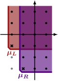
(a) $\mathrm{supp}(\hat{\varphi}_{\mathchoice{\mathbin{\vbox{\hbox{\scalebox{1.0}{$\displaystyle\bullet$}}}}}{\mathbin{\vbox{\hbox{\scalebox{1.0}{$\textstyle\bullet$}}}}}{\mathbin{\vbox{\hbox{\scalebox{1.0}{$\scriptstyle\bullet$}}}}}{\mathbin{\vbox{\hbox{\scalebox{1.0}{$\scriptscriptstyle\bullet$}}}}}})$

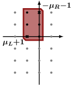
(b) $\rho_{0}$

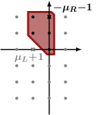
(c) $\rho_{1}$

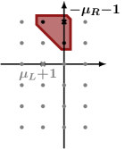
(d) $\rho_{2}$

Figure 3: Supports of the $\hat{\varphi}_{L}$ and $\hat{\varphi}_{R}$ expansions (110) in LABEL:sub@fig:cone-lr, and the corresponding summation domains for eqs. (115, 118) in (LABEL:sub@fig:cone-rho0, LABEL:sub@fig:cone-rho1, LABEL:sub@fig:cone-rho2).

(a) $\mathrm{supp}(u)$

(b) $\mathrm{supp}(\tilde{u})$

(c) $\mathrm{supp}(\tilde{u}^{2})$

(d) for eq. (118)

Figure 4: Supports of the expansions (111) in (LABEL:sub@fig:cone-u0, LABEL:sub@fig:cone-u1, LABEL:sub@fig:cone-u2), where we implicitely assume an extra ${\boldsymbol{i}}\geq{\boldsymbol{0}}$ condition. In (LABEL:sub@fig:cone-u-1) we illustrate the notation of eq. (118) (an additional ${\boldsymbol{i}}\leq{\boldsymbol{0}}$ here is implied as well).

According to the integral formula (32), our goal is to compute the following residue:

$$\rho:={\rm Res}_{z=0}\Bigl{[}\varphi_{R}u^{-1}\int^{z}\varphi_{L}u\Bigr{]}$$ (113)

The key idea is to expand the inverse of the twist $u(z)^{-1}$ in terms of $\tilde{u}(z)$ using the geometric series:

$$\rho =\underbrace{{\rm Res}_{z=0}\Bigl{[}\varphi_{R}\int\varphi_{L}\Bigr{]}}_{\rho_{0}}+\sum_{m=1}^{(-{\boldsymbol{\mu_{L}}}-{\boldsymbol{\mu_{R}}}-{\boldsymbol{2}})\cdot{\boldsymbol{1}}}(-1)^{m}\>\underbrace{{\rm Res}_{z=0}\Bigl{[}\varphi_{R}\cdot\tilde{u}^{m-1}\cdot\Bigl{(}\tilde{u}\int\varphi_{L}-\int\tilde{u}\varphi_{L}\Bigr{)}\Bigr{]}}_{\rho_{m}}\ ,$$ (114)

where in $\rho_{m}$ we gather the residues with $m$ insertions of $\tilde{u}(z)$. The summation bounds in the second term follows from the fact that the $z$-expansion of $\tilde{u}(z)^{m}$ has terms with at least $m$ powers of $z$ inside, as reflected in Figure 4b and Figure 4c for $m=1$ and $m=2$ respectively.

The residue $\rho_{0}$ in eq. (114) is straightforward to evaluate:

$$\rho_{0}=\sum_{{\boldsymbol{i}}={\boldsymbol{\mu_{L}}}+{\boldsymbol{1}}}^{-{\boldsymbol{\mu_{R}}}-{\boldsymbol{1}}}\hat{\varphi}_{R,-{\boldsymbol{i}}-{\boldsymbol{1}}}\>\hat{\varphi}_{L,{\boldsymbol{i}}-{\boldsymbol{1}}}\>\frac{1}{{\boldsymbol{i}}+{\boldsymbol{\gamma}}}\ ,$$ (115)

where the fraction stands for $1/({\boldsymbol{i}}+{\boldsymbol{\gamma}}):=1/\prod_{j}(i_{j}+\gamma_{j})$ , and the $n$-dimensional summation domain is shown in Figure 3b.

To compute $\rho_{m}$ in eq. (114) we separately expand its three factors, multiply them, and take the residue. The first factor is given in eq. (110). The second factor is a power of a series, so we may write its ${\boldsymbol{i}}$^th non-zero coefficient $\tilde{u}(z)^{m}=\sum_{\boldsymbol{i}}(\tilde{u}^{m})_{\boldsymbol{i}}\>z^{\boldsymbol{i}}$ using the Kronecker symbol $\delta_{{\boldsymbol{i}},{\boldsymbol{j}}}$ as:

$$\bigl{(}\tilde{u}^{m}\bigr{)}_{\boldsymbol{i}}=\sum_{{{\boldsymbol{j_{1}}}\cdot{\boldsymbol{1}}}\geq 1}\ldots\sum_{{{\boldsymbol{j_{m}}}}\cdot{\boldsymbol{1}}\geq 1}\delta_{(\sum_{k}{\boldsymbol{j_{k}}}),{\boldsymbol{i}}}\>u_{\boldsymbol{j_{1}}}\ldots u_{\boldsymbol{j_{m}}}\ ,\quad\text{for ${{{\boldsymbol{i}}\cdot{\boldsymbol{1}}}\geq m}$ and ${\boldsymbol{i}}\geq{\boldsymbol{0}}$}\ .$$ (116)

One can come up with various evaluation strategies for this multiple sum using, for example, the nested parametrization as in eq. (158), or the (precomputed) multivariate Bell polynomials Withers:2008 . For the ${\boldsymbol{i}}$^th non-zero coefficient of the last factor of $\rho_{m}$ we get

$$\Bigl{(}\tilde{u}\int\varphi_{L}-\int\tilde{u}\varphi_{L}\Bigr{)}_{\boldsymbol{i}}=\sum_{\begin{subarray}{c}{{\boldsymbol{j}}\cdot{\boldsymbol{1}}}\geq 1\\ {\boldsymbol{j}}\leq{\boldsymbol{i}}-{\boldsymbol{\mu_{L}}}-{\boldsymbol{1}}\end{subarray}}u_{\boldsymbol{j}}\>\hat{\varphi}_{L,{\boldsymbol{i}}-{\boldsymbol{j}}-{\boldsymbol{1}}}\>\Bigl{(}\tfrac{1}{{\boldsymbol{i}}-{\boldsymbol{j}}+{\boldsymbol{\gamma}}}-\tfrac{1}{{\boldsymbol{i}}+{\boldsymbol{\gamma}}}\Bigr{)}\ ,\quad\text{for ${({\boldsymbol{i}}-{\boldsymbol{\mu_{L}}}-{\boldsymbol{1}})\cdot{\boldsymbol{1}}\geq 1}$}$$ (117)

and ${\boldsymbol{i}}\geq{\boldsymbol{\mu_{L}}}+{\boldsymbol{1}}$. Integrals here are done via the same technique as discussed in Section 2.4.

Finally the sum representation of the $\rho_{m}$ residue reads:

$$\rho_{m}=\sum_{\begin{subarray}{c}({\boldsymbol{i}}-{\boldsymbol{\mu_{L}}}-{\boldsymbol{1}})\cdot{\boldsymbol{1}}\geq m\\ {\boldsymbol{i}}\leq-{\boldsymbol{\mu_{R}}}-{\boldsymbol{1}}\end{subarray}}\hat{\varphi}_{R,-{\boldsymbol{i}}-{\boldsymbol{1}}}\sum_{\begin{subarray}{c}{{\boldsymbol{j}}}\cdot{\boldsymbol{1}}\geq m-1\\ ({\boldsymbol{j}}-{\boldsymbol{i}}+{\boldsymbol{\mu_{L}}}+{\boldsymbol{1}})\cdot{\boldsymbol{1}}\leq-1\end{subarray}}(\tilde{u}^{m-1})_{\boldsymbol{j}}\Bigl{(}\tilde{u}\int\varphi_{L}-\int\tilde{u}\varphi_{L}\Bigr{)}_{{\boldsymbol{i}}-{\boldsymbol{j}}}\ ,$$ (118)

where examples of the outer sum’s domain are shown in figures 3c and 3d (see also Figure 4d for an illustration of the $\leq$ notation in the inner sum). Alongside the non-vanishing condition:

$$-{\boldsymbol{\mu_{L}}}-{\boldsymbol{\mu_{R}}}-{\boldsymbol{2}}\geq{\boldsymbol{0}}\ ,$$ (119)

we obtain the algebraic expression for a given residue:

$$\boxed{{\rm Res}(\psi\varphi_{R})=\sum_{m=0}^{(-{\boldsymbol{\mu_{L}}}-{\boldsymbol{\mu_{R}}}-{\boldsymbol{2}})\cdot{\boldsymbol{1}}}(-1)^{m}\rho_{m}}$$ (120)

with $\rho_{m}$ defined by eqs. (115) and (118, 116, 117).

Appendix C Algebraic solution: proof

The purpose of this appendix is to show the validity of the algebraic solution given by eq. (72) and discuss some features not mentioned in the main text.

C.1 Deriving the algebraic expression

We will consider a more general case than in Section 4, and only at the end specify to the “right rescaling” framework. Our starting point will be eqs. (20) and (31):

$$\langle\varphi_{L}\>|\>\varphi_{R}\rangle=\sum_{p\in\mathbb{P}_{\omega}}{\rm Res}_{z=p}(\psi\varphi_{R})$$ (121)

where $\psi$ is defined through

$$\hat{\nabla}_{\omega_{1}}\cdots\hat{\nabla}_{\omega_{n}}\psi=\hat{\varphi}_{L}\qquad\quad\text{where}\qquad\quad\hat{\nabla}_{\omega_{i}}:=\partial_{z_{i}}+(\partial_{z_{i}}\log(u))$$ (122)

We want to approach the differential equation locally as a series expansions. So in the following we will consider a point corresponding to one of the terms of eq. (121) with the assumption that the proper variable changes has been made so $p=0$ and in addition that the series expansions are well defined so no further blowups are needed as also discussed in Section 4.

Let us write the objects involved as such expansions:

$$\hat{\varphi}_{L}=\sum_{\boldsymbol{i}=\boldsymbol{\mu}_{\boldsymbol{L}}}^{\boldsymbol{\infty}}\!\hat{\varphi}_{L,\boldsymbol{i}}\,z^{\boldsymbol{i}}\qquad\qquad\hat{\varphi}_{R}=\sum_{\boldsymbol{i}=\boldsymbol{\mu}_{\boldsymbol{R}}}^{\boldsymbol{\infty}}\!\hat{\varphi}_{R,\boldsymbol{i}}z^{\boldsymbol{i}}\qquad\qquad\psi=\sum_{\boldsymbol{i}=\boldsymbol{\mu}_{\boldsymbol{\psi}}}^{\boldsymbol{\infty}}\!\psi_{\boldsymbol{i}}z^{\boldsymbol{i}}$$ (123)

$$w:=\log(u)=\sum_{\boldsymbol{i}=\boldsymbol{\mu}_{\boldsymbol{w}}}^{\boldsymbol{\infty}}\!w_{\boldsymbol{i}}z^{\boldsymbol{i}}\;+\;\sum_{j=1}^{n}v_{j}\log(z_{j})$$ (124)

The exponent of the leading powers $\boldsymbol{\mu}_{\boldsymbol{L}}$, $\boldsymbol{\mu}_{\boldsymbol{R}}$, $\boldsymbol{\mu}_{\boldsymbol{w}}$ are given by the physical problem, while $\boldsymbol{\mu}_{\boldsymbol{\psi}}$ is not since the $\psi$-expression is an ansatz so $\boldsymbol{\mu}_{\boldsymbol{\psi}}$ is just assumed to chosen to be small enough that all manipulations done in the following are valid.

With these expansions we may easily write the residue we are looking for as

$${\rm Res}_{z=0}(\psi\varphi_{R})=\sum_{\boldsymbol{i}=\boldsymbol{\mu}_{\boldsymbol{\psi}}\!\!}^{-\boldsymbol{\mu}_{\boldsymbol{R}}-\boldsymbol{1}\,}\!\!\!\psi_{\boldsymbol{i}}\,\hat{\varphi}_{R,-\boldsymbol{i}-\boldsymbol{1}}$$ (125)

The challenging part is solving eq. (122) to identify the expressions for the $\psi_{\boldsymbol{i}}$.

C.1.1 The case $n=2$.

Solving the $n$PDE. We first discuss the case $n=2$, and later we extend it to arbitrary $n$-forms. Solving eq. (122) corresponds to solving $\Delta=0$ with

$$\Delta:=\hat{\nabla}_{\omega_{1}}\hat{\nabla}_{\omega_{2}}\psi-\hat{\varphi}_{L}$$ (126)

This corresponds to

$$\Delta =(\partial_{1}\partial_{2}\psi)+(\partial_{1}\partial_{2}w)\psi+(\partial_{1}w)(\partial_{2}\psi)+(\partial_{2}w)(\partial_{1}\psi)+(\partial_{1}w)(\partial_{2}w)\psi-\hat{\varphi}_{L}$$ (127)

where we have used the obvious notation $\partial_{i}:=\partial_{z_{i}}$. Inserting the expansions we get

$$\Delta =\;\,\sum_{\boldsymbol{i}=\boldsymbol{\mu}_{\boldsymbol{\psi}}}^{\boldsymbol{\infty}}(i_{1}i_{2}\psi_{\boldsymbol{i}}-\hat{\varphi}_{L,\boldsymbol{i}-\boldsymbol{1}})z_{1}^{i_{1}-1}z_{2}^{i_{2}-1}$$

$$\;\;+\sum_{\boldsymbol{i}=\boldsymbol{\mu}_{\boldsymbol{\psi}}}^{\boldsymbol{\infty}}\sum_{\boldsymbol{j}=\boldsymbol{\mu}_{\boldsymbol{w}}}^{\boldsymbol{\infty}}\big{(}j_{1}j_{2}w_{\boldsymbol{j}}+i_{2}(j_{1}w_{\boldsymbol{j}}+\delta_{\boldsymbol{j},\boldsymbol{0}}v_{1})+i_{1}(j_{2}w_{\boldsymbol{j}}+\delta_{\boldsymbol{j},\boldsymbol{0}}v_{2})\big{)}\psi_{\boldsymbol{i}}z_{1}^{i_{1}+j_{1}-1}z_{2}^{i_{2}+j_{2}-1}$$

$$\;\;+\sum_{\boldsymbol{i}=\boldsymbol{\mu}_{\boldsymbol{\psi}}}^{\boldsymbol{\infty}}\sum_{\boldsymbol{j}=\boldsymbol{\mu}_{\boldsymbol{w}}}^{\boldsymbol{\infty}}\sum_{\boldsymbol{k}=\boldsymbol{\mu}_{\boldsymbol{w}}}^{\boldsymbol{\infty}}\!(j_{1}w_{\boldsymbol{j}}+\delta_{\boldsymbol{j},\boldsymbol{0}}v_{1})(k_{2}w_{\boldsymbol{k}}+\delta_{\boldsymbol{k},\boldsymbol{0}}v_{2})\psi_{\boldsymbol{i}}\,z_{1}^{i_{1}+j_{1}+k_{1}-1}z_{2}^{i_{2}+j_{2}+k_{2}-1}$$ (128)

Changing the summation variables we may rewrite this as

$$\Delta =\!\!\!\sum_{\boldsymbol{s}=\boldsymbol{\mu}_{\boldsymbol{\psi}}+n\boldsymbol{\mu}_{\boldsymbol{w}}\!}\!\!\!\Delta_{\boldsymbol{s}}\,z^{\boldsymbol{s}-\boldsymbol{1}}$$ (129)

where

$$\Delta_{\boldsymbol{s}} :=\sum_{\boldsymbol{t}=\boldsymbol{\mu}_{\boldsymbol{\psi}}}^{\boldsymbol{s}-n\boldsymbol{\mu}_{\boldsymbol{w}}}\!\!R(\boldsymbol{s}{-}\boldsymbol{t},\boldsymbol{t})\,\psi_{\boldsymbol{t}}\;\;-\;\;\hat{\varphi}_{L,\boldsymbol{s}-\boldsymbol{1}}$$ (130)

with

$$R(\boldsymbol{\alpha},\boldsymbol{\beta}) =(\beta_{1}{+}v_{1})(\beta_{2}{+}v_{2})\delta_{\boldsymbol{\alpha},\boldsymbol{0}}+\big{(}\alpha_{1}\alpha_{2}+\alpha_{1}(\beta_{2}{+}v_{2})+\alpha_{2}(\beta_{1}{+}v_{1})\big{)}w_{\boldsymbol{\alpha}}$$

$$\;\;\;\,+\sum_{\boldsymbol{j}=\boldsymbol{\mu}_{\boldsymbol{w}}}^{\boldsymbol{\alpha}-\boldsymbol{\mu}_{\boldsymbol{w}}}(\alpha_{1}{-}j_{1})j_{2}\,w_{\boldsymbol{\alpha}-\boldsymbol{j}}w_{\boldsymbol{j}}$$ (131)

which reduces to the expression given in eq. (76) in the case where $\boldsymbol{\mu}_{\boldsymbol{w}}=\boldsymbol{0}$. In general this function $R$ may be interpreted as $R(\boldsymbol{\alpha},\boldsymbol{\beta})$ being the coefficient in $\Delta$ of $\psi_{\boldsymbol{\beta}}\,z^{\boldsymbol{\alpha}{+}\boldsymbol{\beta}{-}\boldsymbol{1}}$.

Having $\Delta=0$ in general requires that each term in the $z$-expansion of eq. (129) is zero independently. This means that our task now is to solve $\Delta_{\boldsymbol{s}}=0$ for each value of $\boldsymbol{s}$.

This can be done. If we define

$$\tilde{\boldsymbol{\mu}}_{\boldsymbol{\psi}}:=\boldsymbol{\mu}_{\boldsymbol{L}}-n\boldsymbol{\mu}_{\boldsymbol{w}}+\boldsymbol{1}$$ (132)

we find the recursive solution

$$\psi_{\boldsymbol{q}}\; =\;\qquad\qquad\qquad\qquad\quad 0\qquad\qquad\qquad\qquad\qquad\qquad\text{if}\;\;\boldsymbol{q}\ngeq\tilde{\boldsymbol{\mu}}_{\boldsymbol{\psi}}$$

$$\psi_{\boldsymbol{q}}\; =\;\bigg{(}\hat{\varphi}_{L,\boldsymbol{q}+n\boldsymbol{\mu}_{\boldsymbol{w}}-\boldsymbol{1}}\;-\!\!\!\!\!\sum_{\boldsymbol{r}:\;\tilde{\boldsymbol{\mu}}_{\boldsymbol{\psi}}\leq\boldsymbol{r}<\boldsymbol{q}}\!\!\!\!\!Q(\boldsymbol{q},\boldsymbol{r})\,\psi_{\boldsymbol{r}}\bigg{)}\Big{/}Q(\boldsymbol{q},\boldsymbol{q})\qquad\text{if}\;\;\boldsymbol{q}\geq\tilde{\boldsymbol{\mu}}_{\boldsymbol{\psi}}$$ (133)

where

$$Q(\boldsymbol{q},\boldsymbol{r}):=R(\boldsymbol{q}{-}\boldsymbol{r}{+}n\boldsymbol{\mu}_{\boldsymbol{w}}\,,\;\boldsymbol{r})$$ (134)

and where the exact definitions of $\geq$ and other binary operators applied to the index vectors are given is Section C.4. The quantity $\tilde{\boldsymbol{\mu}}_{\boldsymbol{\psi}}$ may be interpreted as the “correct” value for $\boldsymbol{\mu}_{\boldsymbol{\psi}}$, or at least as a value for which $\boldsymbol{\mu}_{\boldsymbol{\psi}}\nleq\tilde{\boldsymbol{\mu}}_{\boldsymbol{\psi}}$ would make it impossible for the above derivation to go through.

The recursive solution given by eq. (133) can be useful on its own to find $\psi$-solutions to use as arguments of the residue function using for instance eq. (125), but let us continue the derivation in order to find a closed expression.

Evaluation of the residue. The next step is to re-express eq. (133) in a form in which only the coefficients of the individual $\hat{\varphi}_{L,\boldsymbol{i}}$ are recursive. This can be done as

$$\psi_{\boldsymbol{q}} =\sum_{\boldsymbol{\kappa}=\tilde{\boldsymbol{\mu}}_{\boldsymbol{\psi}}}^{\boldsymbol{q}}\!\!\hat{\varphi}_{L,\boldsymbol{\kappa}{+}n\boldsymbol{\mu}_{\boldsymbol{w}}-\boldsymbol{1}}\,\Psi(\boldsymbol{q},\boldsymbol{q}{-}\boldsymbol{\kappa})$$ (135)

with

$$\Psi(\boldsymbol{q},\boldsymbol{\tau})\;=\left\{\begin{array}[]{cc}0&\;\;\text{if}\;\;\boldsymbol{\tau}\ngeq\boldsymbol{0}\\ 1/Q(\boldsymbol{q},\boldsymbol{q})&\;\;\text{if}\;\;\boldsymbol{\tau}=\boldsymbol{0}\\ \frac{-\sum_{\boldsymbol{i}:\,\boldsymbol{0}\leq\boldsymbol{i}<\boldsymbol{\tau}}Q(\boldsymbol{q}{-}\boldsymbol{i},\boldsymbol{q}{-}\boldsymbol{\tau})\Psi(\boldsymbol{q},\boldsymbol{i})}{Q(\boldsymbol{q}{-}\boldsymbol{\tau},\boldsymbol{q}{-}\boldsymbol{\tau})}&\;\;\text{if}\;\;\boldsymbol{\tau}>\boldsymbol{0}\end{array}\right.$$ (139)

or alternatively

$$\Psi(\boldsymbol{q},\boldsymbol{\tau})\;=\left\{\begin{array}[]{cc}0&\;\;\text{if}\;\;\boldsymbol{\tau}\ngeq\boldsymbol{0}\\ 1/W(\boldsymbol{q},\boldsymbol{0})&\;\;\text{if}\;\;\boldsymbol{\tau}=\boldsymbol{0}\\ \frac{-\sum_{\boldsymbol{i}:\,\boldsymbol{0}\leq\boldsymbol{i}<\boldsymbol{\tau}}W(\boldsymbol{q}{-}\boldsymbol{\tau},\boldsymbol{\tau}{-}\boldsymbol{i})\Psi(\boldsymbol{q},\boldsymbol{i})}{W(\boldsymbol{q}{-}\boldsymbol{\tau},\boldsymbol{0})}&\;\;\text{if}\;\;\boldsymbol{\tau}>\boldsymbol{0}\end{array}\right.$$ (143)

where $W(\boldsymbol{\eta},\boldsymbol{\lambda}):=Q(\boldsymbol{\eta}{+}\boldsymbol{\lambda},\boldsymbol{\eta})$ or correspondingly

$$W(\boldsymbol{\eta},\boldsymbol{\lambda}) =R(\boldsymbol{\lambda}{+}n\boldsymbol{\mu}_{\boldsymbol{w}},\,\boldsymbol{\eta})$$ (144)

Eq. (143) is a recursive expression that only involves the coefficients of the expansion of $w$. The recursion can be solved with the result

$$\Psi(\boldsymbol{q},\boldsymbol{\tau}) =\sum_{\sigma\in\text{VC}(\boldsymbol{\tau})}\frac{(-1)^{|\sigma|}}{W(\boldsymbol{q},\boldsymbol{0})}\prod_{i=1}^{|\sigma|}\frac{W(\boldsymbol{q}{-}\boldsymbol{\tau}{+}\sum_{j<i}\boldsymbol{\sigma}_{\boldsymbol{j}},\,\boldsymbol{\sigma}_{\boldsymbol{i}})}{W(\boldsymbol{q}{-}\boldsymbol{\tau}{+}\sum_{j<i}\boldsymbol{\sigma}_{\boldsymbol{j}},\,\boldsymbol{0})}$$ (145)

where VC refers to the vector compositions defined and discussed in Section 4.1. By combining eqs. (135) and (125), and changing the summation variables we get

$$\text{Res}(\psi\varphi_{R}) =\sum_{\boldsymbol{\tau}=\boldsymbol{0}}^{n\boldsymbol{\mu}_{\boldsymbol{w}}-\boldsymbol{\mu}_{\boldsymbol{L}}-\boldsymbol{\mu}_{\boldsymbol{R}}-\boldsymbol{2}\;}\;\;\sum_{\boldsymbol{h}=\tilde{\boldsymbol{\mu}}_{\boldsymbol{\psi}}}^{-\boldsymbol{\mu}_{\boldsymbol{R}}-\boldsymbol{\tau}-\boldsymbol{1}}\!\!\!\;\Psi(\boldsymbol{h}{+}\boldsymbol{\tau},\boldsymbol{\tau})\;\hat{\varphi}_{L,\boldsymbol{h}+n\boldsymbol{\mu}_{\boldsymbol{w}}-\boldsymbol{1}}\;\hat{\varphi}_{R,-\boldsymbol{h}-\boldsymbol{\tau}-\boldsymbol{1}}$$ (146)

and finally we may insert the expression for $\Psi$ from eq. (145) and we get the most general form of the algebraic expression:

$$\boxed{\text{Res}(\psi\varphi_{R})\;=\!\!\!\sum_{\boldsymbol{\tau}=\boldsymbol{0}}^{n\boldsymbol{\mu}_{\boldsymbol{w}}-\boldsymbol{\mu}_{\boldsymbol{L}}-\boldsymbol{\mu}_{\boldsymbol{R}}-\boldsymbol{2}\;}\!\!\!\sum_{\sigma\in\text{VC}(\boldsymbol{\tau})}\;\;\sum_{\boldsymbol{h}=\boldsymbol{\mu}_{\boldsymbol{L}}-n\boldsymbol{\mu}_{\boldsymbol{w}}+\boldsymbol{1}}^{-\boldsymbol{\mu}_{\boldsymbol{R}}-\boldsymbol{\tau}-\boldsymbol{1}}\!\!\!\!\!Y(\boldsymbol{h},\boldsymbol{\tau},\sigma)\;\hat{\varphi}_{L,\boldsymbol{h}+n\boldsymbol{\mu}_{\boldsymbol{w}}-\boldsymbol{1}}\;\hat{\varphi}_{R,-\boldsymbol{h}-\boldsymbol{\tau}-\boldsymbol{1}}}$$ (147)

where

$$Y(\boldsymbol{h},\boldsymbol{\tau},\sigma) :=\frac{(-1)^{|\sigma|}}{W(\boldsymbol{h}{+}\boldsymbol{\tau},\boldsymbol{0})}\prod_{i=1}^{|\sigma|}\frac{W(\boldsymbol{h}{+}\sum_{j<i}\boldsymbol{\sigma}_{\boldsymbol{j}},\,\boldsymbol{\sigma}_{\boldsymbol{i}})}{W(\boldsymbol{h}{+}\sum_{j<i}\boldsymbol{\sigma}_{\boldsymbol{j}},\,\boldsymbol{0})}$$ (148)

We notice that $\boldsymbol{\tau}$ is not really needed as an argument to $Y$ since $\boldsymbol{\tau}=\sum_{j}\boldsymbol{\sigma}_{\boldsymbol{j}}$.

C.1.2 Beyond $n=2$.

Even though the derivation in the previous section was done in the case of $n=2$, it will go through in the same way for different values. In particular the final result eq. (147) will look the same for all values of $n$. The main exceptions are eqs. (126, 127, 128, 131). Looking briefly at some other cases, for $n=1$ we have

$$\Delta\;=\;\hat{\nabla}_{\omega}\psi-\hat{\varphi}_{L}\;=\;(\partial_{z}\psi)+(\partial_{z}w)\psi-\hat{\varphi}_{L}$$ (149)

which will correspond to

$$R(\alpha,\beta)=(\beta{+}v)\delta_{\alpha,0}+\alpha w_{\alpha}$$ (150)

as in eq. (75). Likewise for $n=3$ we have

$$\Delta =\hat{\nabla}_{\omega_{1}}\hat{\nabla}_{\omega_{2}}\hat{\nabla}_{\omega_{3}}\psi-\hat{\varphi}_{L}$$ (151)

$$=(\partial_{1}w)(\partial_{23}\psi)+(\partial_{2}w)(\partial_{13}\psi)+(\partial_{3}w)(\partial_{12}\psi)+(\partial_{12}w)(\partial_{3}\psi)+(\partial_{13}w)(\partial_{2}\psi)+(\partial_{23}w)(\partial_{1}\psi)$$

$$+\big{(}(\partial_{1}w)(\partial_{23}w)+(\partial_{2}w)(\partial_{13}w)+(\partial_{3}w)(\partial_{12}w)\big{)}\psi+(\partial_{1}w)(\partial_{2}w)(\partial_{3}\psi)+(\partial_{1}w)(\partial_{3}w)(\partial_{2}\psi)$$

$$+(\partial_{2}w)(\partial_{3}w)(\partial_{1}\psi)+(\partial_{123}w)\psi+(\partial_{1}w)(\partial_{2}w)(\partial_{3}w)\psi+\partial_{123}\psi-\hat{\varphi}_{L}$$ (152)

which after a similar derivation yields

$$R(\boldsymbol{\alpha},\boldsymbol{\beta}) =\;(\beta_{1}{+}v_{1})(\beta_{2}{+}v_{2})(\beta_{3}{+}v_{3})\delta_{\boldsymbol{\alpha},\boldsymbol{0}}$$

$$\;\;\;+\big{(}(\alpha_{1}{+}\beta_{1}{+}v_{1})(\alpha_{2}{+}\beta_{2}{+}v_{2})(\alpha_{3}{+}\beta_{3}{+}v_{3})-(\beta_{1}{+}v_{1})(\beta_{2}{+}v_{2})(\beta_{3}{+}v_{3})\big{)}w_{\boldsymbol{\alpha}}$$

$$\;\;\;+\;\sum_{\boldsymbol{j}=\boldsymbol{\mu}_{\boldsymbol{w}}}^{\boldsymbol{\alpha}{-}\boldsymbol{\mu}_{\boldsymbol{w}}}\big{(}(\alpha_{1}{-}j_{1})j_{2}(j_{3}{+}\beta_{3}{+}v_{3})+(\alpha_{2}{-}j_{2})j_{3}(j_{1}{+}\beta_{1}{+}v_{1})+(\alpha_{3}{-}j_{3})j_{1}(j_{2}{+}\beta_{2}{+}v_{2})\big{)}w_{\boldsymbol{\alpha}{-}\boldsymbol{j}}w_{\boldsymbol{j}}$$

$$\;\;\;+\,\sum_{\boldsymbol{j}=\boldsymbol{\mu}_{\boldsymbol{w}}}^{\boldsymbol{\alpha}-2\boldsymbol{\mu}_{\boldsymbol{w}}}\,\sum_{\boldsymbol{l}=\boldsymbol{\mu}_{\boldsymbol{w}}}^{\boldsymbol{\alpha}{-}\boldsymbol{j}{-}\boldsymbol{\mu}_{\boldsymbol{w}}}\,(\alpha_{1}{-}j_{1}{-}l_{1})\,j_{2}\,l_{3}\,w_{\boldsymbol{\alpha}{-}\boldsymbol{j}{-}\boldsymbol{l}}\,w_{\boldsymbol{j}}\,w_{\boldsymbol{l}}$$ (153)

which reduces to eq. (77) in the case of $\boldsymbol{\mu}_{\boldsymbol{w}}=\boldsymbol{0}$.

Going through the derivation for various values of $n$ allows us to realize the pattern and find the general expression for $R$ which is given in the following.

General expression for $R$

For $R$ in the $n$-variate case, we may write

$$R(\boldsymbol{\alpha},\boldsymbol{\beta})=\sum_{k=0}^{n}R_{n,k}$$ (154)

where $R_{n,k}$ contains the terms with $k$ $w$-factors and correspondingly $k{-}1$ sums. We find it convenient to use distinct expressions for $R_{n,k}$ for $k=0$, $k=1$, and $k\geq 2$. Defining

$$\lambda_{i}:=\beta_{i}+v_{i}$$ (155)

we have

$$R_{n,0} =\Big{(}\prod_{i=1}^{n}\lambda_{i}\Big{)}\delta_{\boldsymbol{\alpha},\boldsymbol{0}}$$ (156)

$$R_{n,1} =\bigg{(}\Big{(}\prod_{i=1}^{n}(\lambda_{i}{+}\alpha_{i})\Big{)}-\Big{(}\prod_{i=1}^{n}\lambda_{i}\Big{)}\bigg{)}w_{\boldsymbol{\alpha}}$$ (157)

$$R_{n,k} =\!\!\!\sum_{\boldsymbol{i}_{\boldsymbol{2}}=\boldsymbol{\mu}_{\boldsymbol{w}}}^{\boldsymbol{\alpha}-(k-1)\boldsymbol{\mu}_{\boldsymbol{w}}}\cdots\!\!\!\!\!\!\sum_{\boldsymbol{i}_{\boldsymbol{j}}=\boldsymbol{\mu}_{\boldsymbol{w}}}^{\boldsymbol{\alpha}-\sum_{q=2}^{j-1}\boldsymbol{i}_{\boldsymbol{q}}-(k+1-j)\boldsymbol{\mu}_{\boldsymbol{w}}}\!\!\!\!\!\!\cdots\sum_{\boldsymbol{i}_{\boldsymbol{k}}=\boldsymbol{\mu}_{\boldsymbol{w}}}^{\boldsymbol{\alpha}{-}\sum_{q=2}^{k-1}\boldsymbol{i}_{\boldsymbol{q}}-\boldsymbol{\mu}_{\boldsymbol{w}}}$$

$$\quad S_{n,k}\Big{(}\Big{(}\boldsymbol{\alpha}{-}\sum_{q=2}^{k}\boldsymbol{i}_{\boldsymbol{q}}\Big{)},\boldsymbol{i}_{\boldsymbol{2}},\ldots,\boldsymbol{i}_{\boldsymbol{k}},\boldsymbol{\lambda}\Big{)}\,w_{(\boldsymbol{\alpha}{-}\sum_{q=2}^{k}\boldsymbol{i}_{\boldsymbol{q}})}w_{\boldsymbol{i}_{\boldsymbol{2}}}\cdots w_{\boldsymbol{i}_{\boldsymbol{k}}}$$ (158)

where we have defined

$$S_{n,k}(\boldsymbol{i}_{\boldsymbol{1}},\boldsymbol{i}_{\boldsymbol{2}},\ldots,\boldsymbol{i}_{\boldsymbol{k}},\boldsymbol{\lambda}) :=\!\!\!\!\sum_{s\in\text{KSN}(n,k)}\!\!\bigg{(}\prod_{l\in\text{CS}(n,s)}\!\!\!\!\!\!\lambda_{l}\,\bigg{)}\prod_{y=1}^{k}\prod_{j\in s_{y}}i_{y,j}$$ (159)

Here we have $\text{KSN}(n,k)$ being defined as the set of all sets with size $k$ of (non-empty and non-overlapping) subsets of the set of integers from 1 to $n$. An example being

$$\text{KSN}(3,2) =\Big{\{}\big{\{}\{1\},\{2\}\big{\}},\big{\{}\{1\},\{3\}\big{\}},\big{\{}\{2\},\{3\}\big{\}},$$

$$\qquad\big{\{}\{1\},\{2,3\}\big{\}},\big{\{}\{2\},\{1,3\}\big{\}},\big{\{}\{3\},\{1,2\}\big{\}}\Big{\}}$$ (160)

where it should be possible to see the structure reflected in the single-sum term of eq. (153). The other set-function $\text{CS}(n,s)$ gives the counter-set to one of these sets, that is

$$\text{CS}(n,s):=\{1,\ldots,n\}/\bigcup_{i}s_{i}$$ (161)

with an example being

$$\text{CS}(3,\big{\{}\{1\},\{3\}\big{\}}) =\{2\}$$ (162)

We should point out that it is possible to write eq. (158) nicer and more symmetrically at the cost of introducing an extra sum and a delta function, that is

$$R_{n,k} =\!\!\!\sum_{\boldsymbol{i}_{\boldsymbol{1}}=\boldsymbol{\mu}_{\boldsymbol{w}}}^{\boldsymbol{\infty}}\!\!\cdots\!\!\sum_{\boldsymbol{i}_{\boldsymbol{k}}=\boldsymbol{\mu}_{\boldsymbol{w}}}^{\boldsymbol{\infty}}\delta_{(\sum_{j}\!\boldsymbol{i}_{\boldsymbol{j}}),\boldsymbol{\alpha}}\,S_{n,k}(\boldsymbol{i}_{\boldsymbol{1}},\ldots,\boldsymbol{i}_{\boldsymbol{k}},\boldsymbol{\lambda})\,w_{\boldsymbol{i}_{\boldsymbol{1}}}\cdots w_{\boldsymbol{i}_{\boldsymbol{k}}}$$ (163)

where evaluating the $\boldsymbol{i}_{\boldsymbol{1}}$-sum would bring back eq. (158).

C.2 Algebraic expression in the rescaling frameworks

In Section 2.5 it was discussed how to simplify the computation of the intersection number by rescaling the quantities on which it depends, locally at each intersection point. Two different cases were presented, right rescaling and left rescaling, which we will discuss below.

Right rescaling

Right rescaling is defined by the rescalings and renamings given in eq. (37)

$$\hat{\varphi}_{L}\rightarrow\hat{\phi}=\hat{\varphi}_{L}\hat{\varphi}_{R}\,,\qquad\hat{\varphi}_{R}\rightarrow 1\,,\qquad u\rightarrow u_{R}=u/\hat{\varphi}_{R}\,,\qquad\psi\rightarrow f\,.$$ (164)

Eq. (147) may then be used for these rescaled variables, with $\hat{\varphi}_{L,\boldsymbol{i}}$, $\hat{\varphi}_{R,\boldsymbol{i}}$, $w_{\boldsymbol{i}}$, and $v_{j}$ interpreted as the coefficients in the expansions of the rescaled variables $\hat{\phi}$, $1$, and $\log(u_{R})$, and $\boldsymbol{\mu}_{\boldsymbol{L}}$, $\boldsymbol{\mu}_{\boldsymbol{R}}$, $\boldsymbol{\mu}_{\boldsymbol{w}}$ as the corresponding powers of the leading coefficients. But the expansion of $1$ is of course trivial, corresponding to $\hat{\varphi}_{R,\boldsymbol{i}}=\delta_{\boldsymbol{i},\boldsymbol{0}}$ and $\boldsymbol{\mu}_{\boldsymbol{R}}=0$. This allows us to do the $h$-sum of eq. (147) giving

$$\text{Res}(f)\;=\!\!\!\!\!\sum_{\boldsymbol{\tau}=\boldsymbol{0}}^{n\boldsymbol{\mu}_{\boldsymbol{w}}-\boldsymbol{\mu}_{\boldsymbol{L}}-\boldsymbol{2}}\!\!\!\!\sum_{\sigma\in\text{VC}(\boldsymbol{\tau})}\!\!\!\!\!Y(-\boldsymbol{\tau}{-}\boldsymbol{1},\boldsymbol{\tau},\sigma)\;\,\hat{\phi}_{n\boldsymbol{\mu}_{\boldsymbol{w}}-\boldsymbol{\tau}-\boldsymbol{2}}$$ (165)

and inserting the expression for $Y$ the residue becomes

$$\text{Res}(f)\;=\!\!\!\!\!\sum_{\boldsymbol{\tau}=\boldsymbol{0}}^{n\boldsymbol{\mu}_{\boldsymbol{w}}-\boldsymbol{\mu}_{\boldsymbol{L}}-\boldsymbol{2}}\!\!\!\!\sum_{\sigma\in\text{VC}(\boldsymbol{\tau})}\frac{(-1)^{|\sigma|}}{U(\boldsymbol{0},\boldsymbol{0})}\prod_{i=1}^{|\sigma|}\frac{U(\boldsymbol{\sigma}_{\boldsymbol{i}},\,\boldsymbol{\tau}{-}\sum_{j<i}\boldsymbol{\sigma}_{\boldsymbol{j}})}{U(\boldsymbol{0},\,\boldsymbol{\tau}{-}\sum_{j<i}\boldsymbol{\sigma}_{\boldsymbol{j}})}\;\,\hat{\phi}_{n\boldsymbol{\mu}_{\boldsymbol{w}}{-}\boldsymbol{\tau}{-}\boldsymbol{2}}$$ (166)

where

$$U(\boldsymbol{\alpha},\boldsymbol{\beta}) =W(-\boldsymbol{\beta}{-}\boldsymbol{1},\,\boldsymbol{\alpha})$$

$$=R(\boldsymbol{\alpha}{+}n\boldsymbol{\mu}_{\boldsymbol{w}},\,-\boldsymbol{\beta}{-}\boldsymbol{1})$$ (167)

Inserting $\boldsymbol{\mu}_{\boldsymbol{w}}=\boldsymbol{0}$, eq. (166) reduces to the algebraic expression discussed in the main text in eq. (72).

Left rescaling

One may go through the same steps for the left rescaling framework, which is defined in terms of the renamings and rescalings defined in eq. (39)

$$\hat{\varphi}_{L}\rightarrow 1\,,\qquad\hat{\varphi}_{R}\rightarrow\hat{\phi}=\hat{\varphi}_{L}\hat{\varphi}_{R}\,,\qquad u\rightarrow u_{L}=u\hat{\varphi}_{L}\,,\qquad\psi\rightarrow g\,.$$ (168)

Inserting this in eq. (147), we get

$$\text{Res}(g\hat{\varphi}_{L}\hat{\varphi}_{R})\;=\!\!\!\sum_{\boldsymbol{\tau}=\boldsymbol{0}}^{n\boldsymbol{\mu}_{\boldsymbol{w}}-\boldsymbol{\mu}_{\boldsymbol{R}}-\boldsymbol{2}\;}\!\!\!\!\sum_{\sigma\in\text{VC}(\boldsymbol{\tau})}\frac{(-1)^{|\sigma|}}{\tilde{U}(\boldsymbol{0},\boldsymbol{\tau})}\prod_{i=1}^{|\sigma|}\frac{\tilde{U}(\boldsymbol{\sigma}_{\boldsymbol{i}},\,\sum_{j<i}\boldsymbol{\sigma}_{\boldsymbol{j}})}{\tilde{U}(\boldsymbol{0},\,\sum_{j<i}\boldsymbol{\sigma}_{\boldsymbol{j}})}\;\,\hat{\phi}_{n\boldsymbol{\mu}_{\boldsymbol{w}}{-}\boldsymbol{\tau}{-}\boldsymbol{2}}$$ (169)

with

$$\tilde{U}(\boldsymbol{\alpha},\boldsymbol{\beta}) =W(\boldsymbol{\beta}{+}\boldsymbol{1}{-}n\boldsymbol{\mu}_{\boldsymbol{w}},\,\boldsymbol{\alpha})$$

$$=R(\boldsymbol{\alpha}{+}n\boldsymbol{\mu}_{\boldsymbol{w}},\,\boldsymbol{\beta}{+}\boldsymbol{1}{-}n\boldsymbol{\mu}_{\boldsymbol{w}})$$ (170)

Eq. (169) is the algebraic expression in the left rescaling framework.

C.3 Additional details

Expansion maxima

In eqs. (123, 124) we wrote the expansions of $\hat{\varphi}_{L}$, $\hat{\varphi}_{R}$, and $w$ as formal expansions from the corresponding $\boldsymbol{\mu}$ up to $\boldsymbol{\infty}$. Yet we do not need infinitely many terms in the series, there is a maximal value above which the terms do not contribute to the result of eq. (147). Considering eq. (147) as well as the general $n$ expression for $R$ given in and below eq. (154) we may deduce what these maximal values are. Using the notation $\boldsymbol{M}$ in parallel with that used for the minimum values $\boldsymbol{\mu}$ we may write an expansion only containing the terms that are actually needed:

$$\hat{\varphi}_{L}=\sum_{\boldsymbol{i}=\boldsymbol{\mu}_{\boldsymbol{L}}}^{\boldsymbol{M}_{\boldsymbol{L}}}\!\hat{\varphi}_{L,\boldsymbol{i}}z^{\boldsymbol{i}}\qquad\quad\hat{\varphi}_{R}=\sum_{\boldsymbol{i}=\boldsymbol{\mu}_{\boldsymbol{R}}}^{\boldsymbol{M}_{\boldsymbol{R}}}\!\hat{\varphi}_{R,\boldsymbol{i}}z^{\boldsymbol{i}}\qquad\quad w=\sum_{\boldsymbol{i}=\boldsymbol{\mu}_{\boldsymbol{w}}}^{\boldsymbol{M}_{\boldsymbol{w}}\!}\!w_{\boldsymbol{i}}z^{\boldsymbol{i}}\,+\,\sum_{j=1}^{n}v_{j}\log(z_{j})$$ (171)

where we have

$$\boldsymbol{M}_{\boldsymbol{L}}=n\boldsymbol{\mu}_{\boldsymbol{w}}{-}\boldsymbol{\mu}_{\boldsymbol{R}}{-}\boldsymbol{2}\,,\qquad\quad\boldsymbol{M}_{\boldsymbol{R}}=n\boldsymbol{\mu}_{\boldsymbol{w}}{-}\boldsymbol{\mu}_{\boldsymbol{L}}{-}\boldsymbol{2}\,,\qquad\quad\boldsymbol{M}_{\boldsymbol{w}}=(n{+}1)\boldsymbol{\mu}_{\boldsymbol{w}}{-}\boldsymbol{\mu}_{\boldsymbol{L}}{-}\boldsymbol{\mu}_{\boldsymbol{R}}{-}\boldsymbol{2}\,.$$ (172)

This fact is useful for implementation purposes, since it tells which coefficients to extract before applying the algebraic expression. Applying one of the rescaled versions of the algebraic expression does not change these limits if expressed in terms of the original $\varphi_{L}$ and $\varphi_{R}$.

The univariate case

In the univariate case there are two simplifications taking place which deserve discussion. The first is that the vector compositions VC reduce to standard compositions as discussed in Section 4.1. The second is that only one $\omega$ is present which makes it desirable to express the result in terms of expansions of that object, replacing the $w$-expansion of eq. (124) with its separately treated log-terms. That is

$$\omega=\sum_{i=\mu_{\omega}}^{\infty}\!\omega_{i}\,z^{i}$$ (173)

with the relation between the two expansions being $\omega_{i}=(i{+}1)w_{i{+}1}$ except for $\omega_{-1}=v_{1}$. We also have $\mu_{\omega}=\mu_{w}{-}1$. Inserting this in eq. (147) we get

$$\text{Res}(\psi\varphi_{R})\;=\!\!\!\!\sum_{\tau=0}^{\mu_{\omega}-\mu_{\phi}-\mu_{\xi}-1\;}\!\!\!\!\sum_{\sigma\in\text{comp}(\tau)}\;\;\sum_{h=\mu_{\phi}-\mu_{\omega}}^{-\mu_{\xi}-\tau-1}\!\!\!\!\!Y(h,\tau,\sigma)\;\hat{\varphi}_{L,h+\mu_{\omega}}\;\hat{\varphi}_{R,-h-\tau-1}$$ (174)

where

$$Y(h,\tau,\sigma) =\frac{(-1)^{|\sigma|}}{W(h{+}\tau,0)}\prod_{i=1}^{|\sigma|}\frac{W(h{+}\sum_{j<i}\sigma_{j},\,\sigma_{i})}{W(h{+}\sum_{j<i}\sigma_{j},\,0)}$$ (175)

as in eq. (148) but with

$$W(\eta,\lambda)=\eta\,\delta_{\lambda+\mu_{\omega},-1}+\omega_{\lambda+\mu_{\omega}}$$ (176)

Further discussion

It is worthwhile to look at the special case in which everything (e.g. $\varphi_{L}$, $\varphi_{R}$, and all $\omega_{i}$) has simple poles only. This corresponds to $\boldsymbol{\mu}_{\boldsymbol{L}}=\boldsymbol{\mu}_{\boldsymbol{R}}=\boldsymbol{-1}$ and $\boldsymbol{\mu}_{\boldsymbol{w}}=\boldsymbol{0}$. Inserting this in eq. (147) we get that each of the sums contain one term only, leaving

$$\text{Res}(\psi\varphi_{R}) =\frac{\hat{\varphi}_{L,\boldsymbol{-1}}\,\hat{\varphi}_{R,\boldsymbol{-1}}}{\prod_{i=1}^{n}v_{i}}$$ (177)

Combining this with eq. (20) we get an expression for the intersection number similar to an expression from refs. matsumoto1998 ; Mizera:2017rqa .

Additionally it is worth noticing that that the intersection number is linear in both $\varphi_{L}$ and $\varphi_{R}$ which may be seen from the integral definition in eq. (15). That property is easy to see in the algebraic expression as it is given by eq. (147). But in the rescaling framework linearity becomes hidden. For instance looking at the solution in the right-rescaling framework as it is given by eq. (72), linearity in $\varphi_{L}$ is obvious. Linearity in $\varphi_{R}$, however, becomes obscured as the $\varphi_{R,\boldsymbol{i}}$-terms mix with the $w_{\boldsymbol{i}}$-factors, which enter the expressions in a very non-linear fashion.

C.4 Comparing index vectors

(a) $\;\boldsymbol{a}\geq\boldsymbol{b}$

(b) $\;\boldsymbol{a}>\boldsymbol{b}$

(c) $\;\boldsymbol{a}\leq\boldsymbol{b}$

(d) $\;\boldsymbol{a}\nleq\boldsymbol{b}$

Figure 5: Illustration of some of the binary operators defined in Table 6. The shaded areas cover the integer values for which the illustrated relation is true.

$\boldsymbol{a}=\boldsymbol{b}$	$\forall i$: $a_{i}=b_{i}$
$\boldsymbol{a}\leq\boldsymbol{b}$	$\forall i$: $a_{i}\leq b_{i}$
$\boldsymbol{a}\geq\boldsymbol{b}$	$\forall i$: $a_{i}\geq b_{i}$
$\boldsymbol{a}<\boldsymbol{b}$	$\boldsymbol{a}\leq\boldsymbol{b}$ and $\boldsymbol{a}\neq\boldsymbol{b}$

$\boldsymbol{a}\neq\boldsymbol{b}$	$\text{not}(\boldsymbol{a}=\boldsymbol{b})$
$\boldsymbol{a}\nleq\boldsymbol{b}$	$\text{not}(\boldsymbol{a}\leq\boldsymbol{b})$
$\boldsymbol{a}\ngeq\boldsymbol{b}$	$\text{not}(\boldsymbol{a}\geq\boldsymbol{b})$
$\boldsymbol{a}>\boldsymbol{b}$	$\boldsymbol{a}\geq\boldsymbol{b}$ and $\boldsymbol{a}\neq\boldsymbol{b}$

Table 6: The definitions needed to compare index vectors.

In this appendix and in Section 4 we used the notation for the $n$-variate formula eq. (72) where the sums and products are parameterized by index vectors written in bold, of length $n$ and containing integers. Such vectors can be compared using the so-called product order, let us briefly review how it is done. If we let $\boldsymbol{a}$ and $\boldsymbol{b}$ be two such index vectors of length $n$, the relations we use in this paper are defined as in Table 6, and some are illustrated in Figure 5. We see that $\nleq$ and $>$ are not equivalent, for instance it is true that $\binom{1}{2}\nleq\binom{2}{0}$ while it is false that $\binom{1}{2}>\binom{2}{0}$. We notice that the index vectors form a partially ordered set under the $\leq$ operator.

References

- (1) K. Matsumoto, Quadratic Identities for Hypergeometric Series of Type , Kyushu Journal of Mathematics 48 (1994), no. 2 335–345.
- (2) K. Matsumoto, Intersection numbers for logarithmic -forms, Osaka J. Math. 35 (1998), no. 4 873–893.
- (3) K. Ohara, Y. Sugiki, and N. Takayama, Quadratic Relations for Generalized Hypergeometric Functions , Funkcialaj Ekvacioj 46 (2003), no. 2 213–251.
- (4) Y. Goto, Twisted Cycles and Twisted Period Relations for Lauricella’s Hypergeometric Function , International Journal of Mathematics 24 (2013), no. 12 1350094, [arXiv:1308.5535].
- (5) Y. Goto and K. Matsumoto, The monodromy representation and twisted period relations for Appell’s hypergeometric function , Nagoya Math. J. 217 (03, 2015) 61–94.
- (6) Y. Goto, Twisted period relations for Lauricella’s hypergeometric functions , Osaka J. Math. 52 (07, 2015) 861–879.
- (7) Y. Goto, Intersection Numbers and Twisted Period Relations for the Generalized Hypergeometric Function , Kyushu Journal of Mathematics 69 (2015), no. 1 203–217.
- (8) S. Mizera, Scattering Amplitudes from Intersection Theory, Phys. Rev. Lett. 120 (2018), no. 14 141602, [arXiv:1711.00469].
- (9) S.-J. Matsubara-Heo and N. Takayama, An algorithm of computing cohomology intersection number of hypergeometric integrals, Nagoya Mathematical Journal (2019) 1–17, [arXiv:1904.01253].
- (10) K. Ohara, “Intersection numbers of twisted cohomology groups associated with Selberg-type integrals.” http://www.math.kobe-u.ac.jp/HOME/ohara/Math/980523.ps, 1998.
- (11) Y. Goto and S.-J. Matsubara-Heo, Homology and cohomology intersection numbers of gkz systems, 2020.
- (12) S.-J. Matsubara-Heo, Computing cohomology intersection numbers of gkz hypergeometric systems, 2020.
- (13) S.-J. Matsubara-Heo, Localization formulas of cohomology intersection numbers, 2021.
- (14) P. Mastrolia and S. Mizera, Feynman Integrals and Intersection Theory, JHEP 02 (2019) 139, [arXiv:1810.03818].
- (15) H. Frellesvig, F. Gasparotto, S. Laporta, M. K. Mandal, P. Mastrolia, L. Mattiazzi, and S. Mizera, Decomposition of Feynman Integrals on the Maximal Cut by Intersection Numbers, JHEP 05 (2019) 153, [arXiv:1901.11510].
- (16) H. Frellesvig, F. Gasparotto, M. K. Mandal, P. Mastrolia, L. Mattiazzi, and S. Mizera, Vector Space of Feynman Integrals and Multivariate Intersection Numbers, Phys. Rev. Lett. 123 (2019), no. 20 201602, [arXiv:1907.02000].
- (17) H. Frellesvig, F. Gasparotto, S. Laporta, M. K. Mandal, P. Mastrolia, L. Mattiazzi, and S. Mizera, Decomposition of Feynman Integrals by Multivariate Intersection Numbers, JHEP 03 (2021) 027, [arXiv:2008.04823].
- (18) K. Aomoto and M. Kita, Theory of Hypergeometric Functions. Springer Monographs in Mathematics. Springer Japan, 2011.
- (19) S. Mizera and A. Pokraka, From Infinity to Four Dimensions: Higher Residue Pairings and Feynman Integrals, JHEP 02 (2020) 159, [arXiv:1910.11852].
- (20) J. Chen, X. Jiang, X. Xu, and L. L. Yang, Constructing canonical Feynman integrals with intersection theory, Phys. Lett. B 814 (2021) 136085, [arXiv:2008.03045].
- (21) S. Weinzierl, Applications of intersection numbers in physics, in MathemAmplitudes 2019: Intersection Theory and Feynman Integrals, 11, 2020. arXiv:2011.02865.
- (22) S. Caron-Huot and A. Pokraka, Duals of Feynman integrals. Part I. Differential equations, JHEP 12 (2021) 045, [arXiv:2104.06898].
- (23) S. Caron-Huot and A. Pokraka, Duals of Feynman Integrals. Part II. Generalized unitarity, JHEP 04 (2022) 078, [arXiv:2112.00055].
- (24) J. Chen, X. Jiang, C. Ma, X. Xu, and L. L. Yang, Baikov representations, intersection theory, and canonical Feynman integrals, JHEP 07 (2022) 066, [arXiv:2202.08127].
- (25) S. Mizera, Status of Intersection Theory and Feynman Integrals, PoS MA2019 (2019) 016, [arXiv:2002.10476].
- (26) S. L. Cacciatori, M. Conti, and S. Trevisan, Co-Homology of Differential Forms and Feynman Diagrams, Universe 7 (2021), no. 9 328, [arXiv:2107.14721].
- (27) S. Abreu, R. Britto, and C. Duhr, The SAGEX Review on Scattering Amplitudes, Chapter 3: Mathematical structures in Feynman integrals, arXiv:2203.13014.
- (28) S. Weinzierl, Feynman Integrals, arXiv:2201.03593.
- (29) P. Mastrolia, From Diagrammar to Diagrammalgebra, PoS MA2019 (2022) 015.
- (30) H. A. Frellesvig and L. Mattiazzi, On the Application of Intersection Theory to Feynman Integrals: the univariate case, PoS MA2019 (2022) 017, [arXiv:2102.01576].
- (31) M. K. Mandal and F. Gasparotto, On the Application of Intersection Theory to Feynman Integrals: the multivariate case, PoS MA2019 (2022) 019.
- (32) C. Ma, Y. Wang, X. Xu, L. L. Yang, and B. Zhou, Mixed QCD-EW corrections for Higgs leptonic decay via vertex, JHEP 09 (2021) 114, [arXiv:2105.06316].
- (33) S. Abreu, R. Britto, C. Duhr, E. Gardi, and J. Matthew, From positive geometries to a coaction on hypergeometric functions, JHEP 02 (2020) 122, [arXiv:1910.08358].
- (34) S. Abreu, R. Britto, C. Duhr, E. Gardi, and J. Matthew, Generalized hypergeometric functions and intersection theory for Feynman integrals, PoS (2019), no. RACOR2019 067, [arXiv:1912.03205].
- (35) S. Abreu, R. Britto, C. Duhr, E. Gardi, and J. Matthew, The diagrammatic coaction beyond one loop, JHEP 10 (2021) 131, [arXiv:2106.01280].
- (36) S. Abreu, R. Britto, C. Duhr, E. Gardi, and J. Matthew, The Diagrammatic Coaction, in 16th DESY Workshop on Elementary Particle Physics: Loops and Legs in Quantum Field Theory 2022, 7, 2022. arXiv:2207.07843.
- (37) S. Mizera, Combinatorics and Topology of Kawai-Lewellen-Tye Relations, JHEP 08 (2017) 097, [arXiv:1706.08527].
- (38) A. Kaderli, A note on the Drinfeld associator for genus-zero superstring amplitudes in twisted de Rham theory, J. Phys. A 53 (2020), no. 41 415401, [arXiv:1912.09406].
- (39) N. Kalyanapuram and R. G. Jha, Positive Geometries for all Scalar Theories from Twisted Intersection Theory, Phys. Rev. Res. 2 (2020), no. 3 033119, [arXiv:2006.15359].
- (40) S. Weinzierl, Correlation functions on the lattice and twisted cocycles, Phys. Lett. B 805 (2020) 135449, [arXiv:2003.05839].
- (41) K. Cho and K. Matsumoto, Intersection theory for twisted cohomologies and twisted Riemann’s period relations I, Nagoya Math. J. 139 (1995) 67–86.
- (42) S. Mizera, Aspects of Scattering Amplitudes and Moduli Space Localization, arXiv:1906.02099.
- (43) S. Weinzierl, On the computation of intersection numbers for twisted cocycles, J. Math. Phys. 62 (2021), no. 7 072301, [arXiv:2002.01930].
- (44) K. Matsumoto, Relative twisted homology and cohomology groups associated with Lauricella’s , arXiv:1804.00366.
- (45) S.-J. Matsubara-Heo and N. Takayama, Algorithms for pfaffian systems and cohomology intersection numbers of hypergeometric integrals, in Lecture Notes in Computer Science, Lecture notes in computer science, pp. 73–84. Springer International Publishing, 2020. Errata in http://www.math.kobe-u.ac.jp/OpenXM/Math/intersection2/.
- (46) V. Chestnov, F. Gasparotto, M. K. Mandal, P. Mastrolia, S. J. Matsubara-Heo, H. J. Munch, and N. Takayama, Macaulay Matrix for Feynman Integrals: Linear Relations and Intersection Numbers, arXiv:2204.12983.
- (47) P. A. Baikov, Explicit solutions of the multiloop integral recurrence relations and its application, Nucl. Instrum. Meth. A389 (1997) 347–349, [hep-ph/9611449].
- (48) E. Witten, Analytic Continuation Of Chern-Simons Theory, AMS/IP Stud. Adv. Math. 50 (2011) 347–446, [arXiv:1001.2933].
- (49) R. N. Lee and A. A. Pomeransky, Critical points and number of master integrals, JHEP 11 (2013) 165, [arXiv:1308.6676].
- (50) T. Bitoun, C. Bogner, R. P. Klausen, and E. Panzer, Feynman integral relations from parametric annihilators, Lett. Math. Phys. 109 (2019), no. 3 497–564, [arXiv:1712.09215].
- (51) D. Agostini, C. Fevola, A.-L. Sattelberger, and S. Telen, Vector Spaces of Generalized Euler Integrals, arXiv:2208.08967.
- (52) F. V. Tkachov, A Theorem on Analytical Calculability of Four Loop Renormalization Group Functions, Phys. Lett. B 100 (1981) 65–68.
- (53) K. G. Chetyrkin and F. V. Tkachov, Integration by Parts: The Algorithm to Calculate beta Functions in 4 Loops, Nucl. Phys. B192 (1981) 159–204.
- (54) S. Laporta, High precision calculation of multiloop Feynman integrals by difference equations, Int. J. Mod. Phys. A15 (2000) 5087–5159, [hep-ph/0102033].
- (55) P. Griffiths and J. Harris, Principles of algebraic geometry. Wiley Classics Library. John Wiley & Sons, Nashville, TN, Aug., 1994.
- (56) S. Borowka, G. Heinrich, S. Jahn, S. P. Jones, M. Kerner, J. Schlenk, and T. Zirke, pySecDec: a toolbox for the numerical evaluation of multi-scale integrals, Comput. Phys. Commun. 222 (2018) 313–326, [arXiv:1703.09692].
- (57) G. Heinrich, S. Jahn, S. P. Jones, M. Kerner, F. Langer, V. Magerya, A. Pöldaru, J. Schlenk, and E. Villa, Expansion by regions with pySecDec, Comput. Phys. Commun. 273 (2022) 108267, [arXiv:2108.10807].
- (58) C. Bogner and S. Weinzierl, Resolution of singularities for multi-loop integrals, Comput. Phys. Commun. 178 (2008) 596–610, [arXiv:0709.4092].
- (59) G. E. Andrews, The Theory of Partitions. Encyclopedia of Mathematics and its Applications. Cambridge University Press, 1984.
- (60) C. S. Withers and S. Nadarajah, Multivariate Bell polynomials and their applications to powers and fractionary iterates of vector power series and to partial derivatives of composite vector functions, Applied Mathematics and Computation 206 (2008), no. 2 997–1004.