Log-correlated color in Monet’s paintings

Abstract

We describe evidence for logarithmic correlations within the paintings of Claude Monet.

Logarithmic correlations appear in a variety of physical models—from statistical mechanics to quantum field theory to turbulence—and play an important role in several fields of pure and applied mathematics—from random matrix theory to number theory to finance [1, 2, 3, 4, 5, 6, 7, 8, 9, 10, 11, 12, 13]. Here, we describe evidence for logarithmic correlations in the world of art.

The two-dimensional Gaussian free field is a simple physical model with logarithmic correlations. On a lattice, the model consists of harmonic springs connecting the height of neighboring lattice sites. A typical equilibrium configuration of this model is shown in Fig. 1. The correlation function takes the form

$$C(r)=\big{\langle}\big{(}h(\mathbf{x})-\langle h\rangle\big{)}\big{(}h(\mathbf{x}^{\prime})-\langle h\rangle\big{)}\big{\rangle}_{\|\mathbf{x}-\mathbf{x}^{\prime}\|=r}\propto\log\frac{r_{0}}{r}$$ (1)

The logarithmic correlations can be seen in averages taken over a single typical configuration. Fig. 2 shows the empirical correlation function derived from averaging over the snapshot in Fig. 1. Logarithmic correlations result in a fractal geometry of fluctuations, along with other rich properties that have been researched extensively [14, 15].

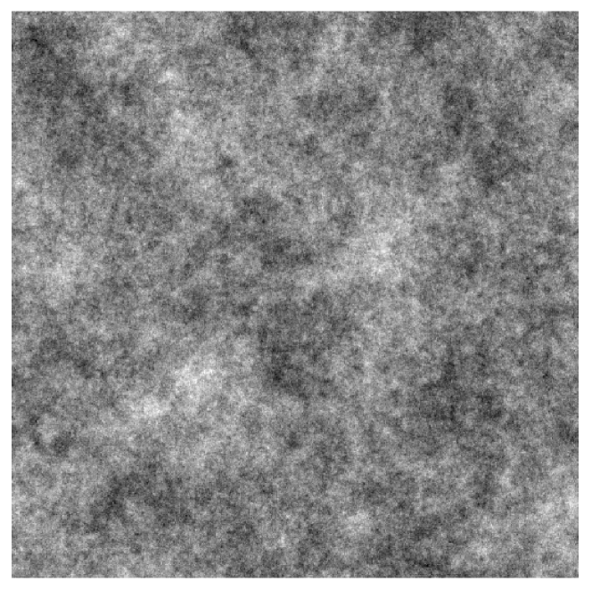
Figure 1: A typical equilibrium configuration of the 2D Gaussian free field on $512\times 512$ square lattice at $T=1$.

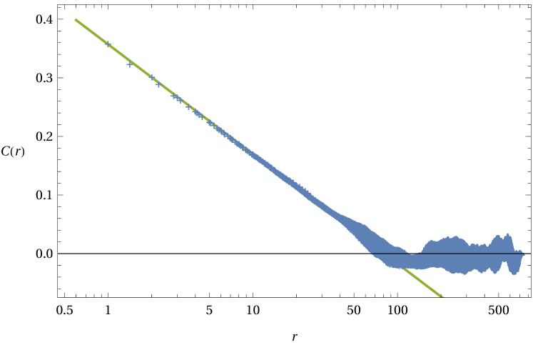
Figure 2: The empirical correlation function of the 2D Gaussian free field resulting from the snapshot in Fig. 1. The green line shows a fit of (1). Logarithms appear linear on a log–linear plot.

Examining Fig. 1, one might notice a superficial similarity with impressionist art. Consider the painting in Fig. 3, The artist’s house seen from the rose garden by Claude Monet. This painting has fluctuations of color that strike the authors as qualitatively alike to that of the Gaussian free field. In the following, we argue that these fluctuations are also quantitatively alike.

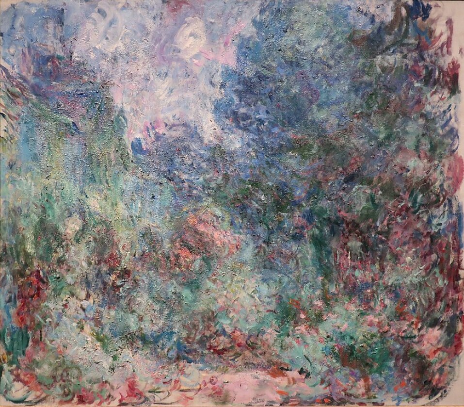
Figure 3: The artist’s house seen from the rose garden, by Claude Monet (1922–1924).

To examine correlations within the painting in Fig. 3, we first convert its pixel color encoding to hue, saturation, and brightness (HSB). Hue, in particular, can be represented as a point on a periodic color line. We extract the hue from the image and encode its value as a vector on the unit circle. Encoded in this way, the hue of the image is equivalent to a state of the xy model on a square lattice. This allows us to define the correlation function

$$C(\mathbf{r})=\big{\langle}\mathbf{h}(\mathbf{x})\cdot\mathbf{h}(\mathbf{x}^{\prime})\big{\rangle}_{\mathbf{r}=|\mathbf{x}-\mathbf{x}^{\prime}|}$$ (2)

The resulting correlation function is plotted in Fig. 5, along with a logarithmic fit. Remarkably, the correlations in the hue are described extremely well by a logarithm with a short-distance cutoff. The horizontal and vertical directions in this painting have nearly identical correlations.

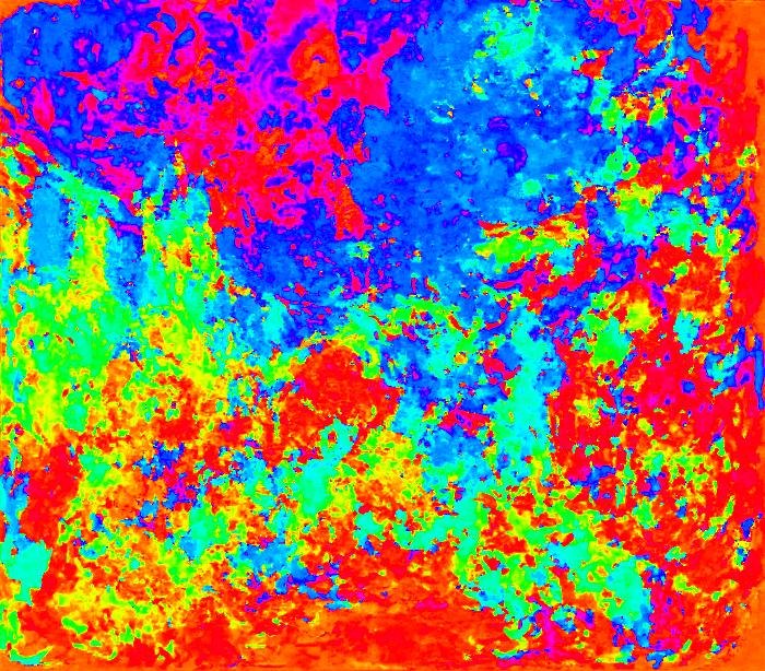
Figure 4: The hue field of the painting in Fig. 3, created by uniformly setting the brightness and saturation to one.

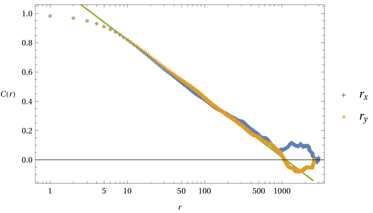
Figure 5: The correlation function along the horizontal ($\mathbf{r}=r_{x}\hat{\mathbf{x}}$) and vertical ($\mathbf{r}=r_{y}\hat{\mathbf{y}}$) for the hue field of the painting in Fig. 3. The line shows a fit of a logarithmic decay.

In order to further investigate this, we chose a collection of Monet paintings in similar style, all painted in the late part of the artist’s life. These were all analysed as described above, with correlation functions plotted in Fig. 6 and fit to logarithms with a short-distance cutoff. Most of the paintings have some scale at which the logarithmic correlations describe the behavior reasonably well, but the quality of the logarithmic description varies substantially from painting to painting.

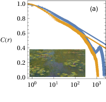
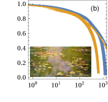
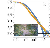
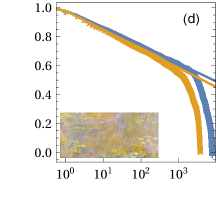
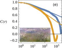
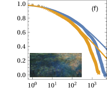
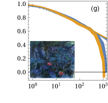
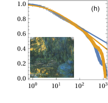
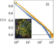
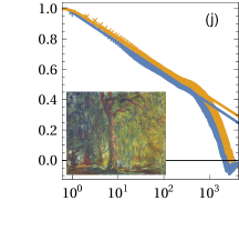
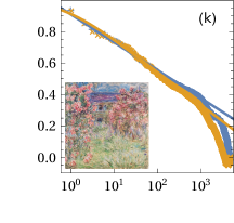
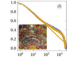
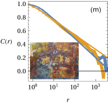
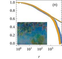
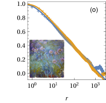
Figure 6: Correlation functions in the horizontal (blue) and vertical (orange) directions, along with fits of cutoff logarithms, for a variety of Monet paintings. The paintings are, from left to right and top to bottom, (a) Le bassin aux nymphéas (1919), (b) Water lilies (1919), (c) Water lilies (1917–1919), (d) Water lilies (1920), (e) Water lilies (c. 1915–1926), (f) Reflection of clouds on the water-lily pond (c. 1920), (g) Water lilies and reflections of a willow (1916–1919), (h) Water-lily pond and weeping willow (1916–1919), (i) Weeping willow (1918), (j) Weeping willow (1918–1919), (k) House among the roses (1917–1919), (l) The rose walk, Giverny (1920–1922), (m) The Japanese footbridge (1920–1922), (n) Wisteria (1920–1925), (o) Agopanthus (1914–1926), and (p) Water lilies (c. 1915).

Fig. 7 compares paintings with the best and worst descriptions by log correlations. Certain qualitative features can be identified by eye: the paintings with stronger log correlations seem to have more color variations at short and medium length scales, while those with weak log correlations have large regions of slow color variation with sharper boundaries. Paintings with stronger log correlations also appear more abstract.

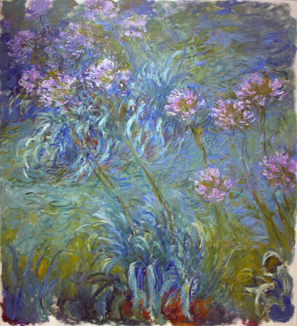
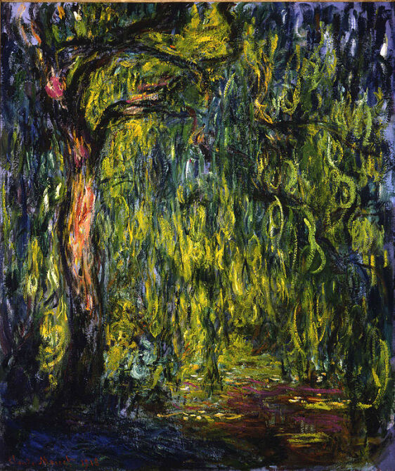
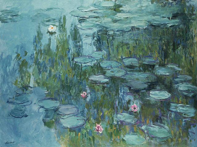
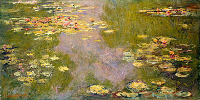
Figure 7: Examples of the Monet paintings in Fig. 6 the strongest and weakest log correlation. Top: Paintings with the strongest log correlation: Agopanthus (1914–1926) and Weeping willow (1918). Bottom: Paintings with the weakest log correlation: Water lilies (c. 1915) and Water lilies (1919).

It’s known that photographs of natural scenes have fluctuations characteristic of logarithmic correlations [16, 17, 18]. Could it be that Claude Monet has just faithfully reproduced these actually occurring statistics in the natural scenes he depicted? To investigate this, we preformed the same analysis with several photographs of Monet’s gardens in Giverny taken by the author or his wife, shown in Fig. 8. Like other natural images, these photos exhibit varying levels of log correlations, or at least their signature. This suggests that Monet is capturing the real correlations in the scenes he depicts, and in his more abstract work amplifies them dramatically.

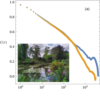
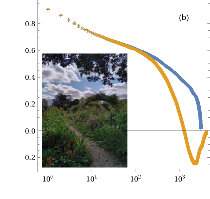
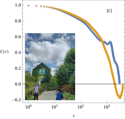
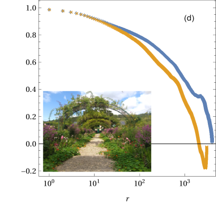
Figure 8: Correlation functions in the horizontal (blue) and vertical (orange) directions for several photographs of Claude Monet’s gardens in Giverny. These photos were taken by the author or his wife on August 19th 2021. (a) The lily pond from the south bank. (b) The gardens from the artist’s house. (c) The artist’s house from the rose garden. (d) The artist’s house through the trestles.

Despite the common belief that beauty is subjective, attempts have been made to quantify the beauty of art. In work by Lakhal et al. [19], the authors propose that structural complexity could be such a measure. They had people compare randomly generated images with particular spatial correlations; log correlations correspond to their parameter $\alpha=-1$. They found that the people surveyed found log correlated images to be among the most attractive, perhaps because of their statistical connection to natural images. Therefore, one might reason that much of wildly-appreciated art would contain log correlations. What makes some of these Monet paintings so striking is how well-described their correlations are by logarithms alone.

Many of the Monet paintings with strong log correlations seem to have been done during the period 1914–1925, a time when the artist suffered from cataracts affecting his vision [20, 21]. At the beginning of this period, he reported that “colours no longer had the same intensity for me,” “reds had begun to look muddy,” and “my painting was getting more and more darkened.” His work took on a broader style with more intense colors, epitomized by Fig. 3. Perhaps Monet’s cataracts affected his painting by leading him to emphasize the abstract (log-correlated) beauty in the strokes of paint over the literal (less log-correlated) beauty of the scene they were meant to depict. However, after 1923–1925 when his cataracts were surgically treated, Monet destroyed many of his paintings from the preceding period and returned to an earlier style. This suggests that the log correlations alone were not enough to meet Monet’s own standard of beauty.

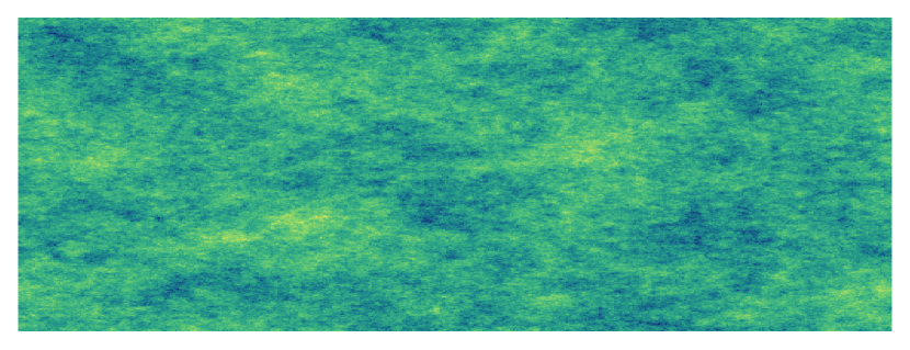
Figure 9: The same Gaussian free field as in Fig. 1, but scaled anisotropically and colored using the Mathematica BlueGreenYellow color scheme.

The presence of logarithmic correlations within Monet paintings suggests a method for producing new Monet-like graphics. First, a log-correlated configuration of some system is produced by standard means. Then, the field is colored using a suitable palette, and perhaps stretched or squished to produce effective anisotropy between horizontal and vertical directions. A first attempt to produce such an image is found in Fig. 9, which the authors feel has a passing resemblance to some of Monet’s work. Incorporating the appropriate brightness and saturation fluctuations would likely improve the resemblance further.

Funding information

JK-D is supported by the Simons Foundation Grant No. 454943.

References

- [1] Nathanaël Berestycki “Introduction to the Gaussian free field and Liouville quantum gravity” In Lecture notes, 2015 URL: https://warwick.ac.uk/fac/sci/maths/research/events/seminars/areas/sis/2018-19/oxford5_berestycki.pdf
- [2] David Carpentier and Pierre Le Doussal “Glass transition of a particle in a random potential, front selection in nonlinear renormalization group, and entropic phenomena in Liouville and sinh-Gordon models” In Physical Review E 63.2 American Physical Society (APS), 2001, pp. 026110 DOI: 10.1103/physreve.63.026110
- [3] Bertrand Duplantier, Rémi Rhodes, Scott Sheffield and Vincent Vargas “Log-correlated Gaussian Fields: An Overview” In Geometry, Analysis and Probability 310, Progress in Mathematics Springer International Publishing, 2017, pp. 191–216 DOI: 10.1007/978-3-319-49638-2_9
- [4] Yan V. Fyodorov and Pierre Le Doussal “Moments of the Position of the Maximum for GUE Characteristic Polynomials and for Log-Correlated Gaussian Processes” In Journal of Statistical Physics 164.1 Springer ScienceBusiness Media LLC, 2016, pp. 190–240 DOI: 10.1007/s10955-016-1536-6
- [5] Yan V. Fyodorov and Jonathan P. Keating “Freezing transitions and extreme values: random matrix theory, and disordered landscapes” In Philosophical Transactions of the Royal Society A: Mathematical, Physical and Engineering Sciences 372.2007 The Royal Society, 2014, pp. 20120503 DOI: 10.1098/rsta.2012.0503
- [6] Y.. Fyodorov, B.. Khoruzhenko and N.. Simm “Fractional Brownian motion with Hurst index and the Gaussian Unitary Ensemble” In The Annals of Probability 44.4 Institute of Mathematical Statistics, 2016, pp. 2980–3031 DOI: 10.1214/15-aop1039
- [7] Nicola Kistler “Derrida’s random energy models. From spin glasses to the extremes of correlated random fields”, 2014 arXiv: http://arxiv.org/abs/1412.0958v1
- [8] Rémi Rhodes and Vincent Vargas “Gaussian multiplicative chaos and applications: A review” In Probability Surveys 11 Institute of Mathematical Statistics, 2014, pp. 315–392 DOI: 10.1214/13-ps218
- [9] E C Bailey and J P Keating “Maxima of log-correlated fields: some recent developments” In Journal of Physics A: Mathematical and Theoretical 55.5 IOP Publishing, 2022, pp. 053001 DOI: 10.1088/1751-8121/ac4394
- [10] Xiangyu Cao, Yan V. Fyodorov and Pierre Le Doussal “Log-correlated random-energy models with extensive free-energy fluctuations: Pathologies caused by rare events as signatures of phase transitions” In Physical Review E 97.2 American Physical Society (APS), 2018, pp. 022117 DOI: 10.1103/physreve.97.022117
- [11] Yan V. Fyodorov and Pierre Le Doussal “Statistics of Extremes in Eigenvalue-Counting Staircases” In Physical Review Letters 124.21 American Physical Society (APS), 2020, pp. 210602 DOI: 10.1103/physrevlett.124.210602
- [12] Yan V. Fyodorov, Ghaith A. Hiary and Jonathan P. Keating “Freezing Transition, Characteristic Polynomials of Random Matrices, and the Riemann Zeta Function” In Physical Review Letters 108.17 American Physical Society (APS), 2012, pp. 170601 DOI: 10.1103/physrevlett.108.170601
- [13] Scott Sheffield “Gaussian free fields for mathematicians” In Probability Theory and Related Fields 139.3-4 Springer ScienceBusiness Media LLC, 2007, pp. 521–541 DOI: 10.1007/s00440-006-0050-1
- [14] E. Bacry, A. Kozhemyak and J.. Muzy “Log-normal continuous cascade model of asset returns: aggregation properties and estimation” In Quantitative Finance 13.5 Informa UK Limited, 2013, pp. 795–818 DOI: 10.1080/14697688.2011.647411
- [15] Jean Duchon, Raoul Robert and Vincent Vargas “FORECASTING VOLATILITY WITH THE MULTIFRACTAL RANDOM WALK MODEL” In Mathematical Finance 22.1 Wiley, 2010, pp. 83–108 DOI: 10.1111/j.1467-9965.2010.00458.x
- [16] Daniel L Ruderman “The statistics of natural images” In Network: Computation in Neural Systems 5.4 Informa UK Limited, 1994, pp. 517–548 DOI: 10.1088/0954-898x_5_4_006
- [17] Daniel L. Ruderman and William Bialek “Statistics of natural images: Scaling in the woods” In Physical Review Letters 73.6 American Physical Society (APS), 1994, pp. 814–817 DOI: 10.1103/physrevlett.73.814
- [18] Greg J. Stephens, Thierry Mora, Gašper Tkačik and William Bialek “Statistical Thermodynamics of Natural Images” In Physical Review Letters 110.1 American Physical Society (APS), 2013, pp. 018701 DOI: 10.1103/physrevlett.110.018701
- [19] Samy Lakhal, Alexandre Darmon, Jean-Philippe Bouchaud and Michael Benzaquen “Beauty and structural complexity” In Physical Review Research 2.2 American Physical Society (APS), 2020, pp. 022058 DOI: 10.1103/physrevresearch.2.022058
- [20] Anna Gruener “The effect of cataracts and cataract surgery on Claude Monet” In British Journal of General Practice 65.634 Royal College of General Practitioners, 2015, pp. 254–255 DOI: 10.3399/bjgp15x684949
- [21] Michael F. Marmor “Ophthalmology and Art: Simulation of Monet’s Cataracts and Degas’ Retinal Disease” In Archives of Ophthalmology 124.12 American Medical Association (AMA), 2006, pp. 1764 DOI: 10.1001/archopht.124.12.1764