A smooth basis for atomistic machine learning

Abstract

Machine learning frameworks based on correlations of interatomic positions begin with a discretized description of the density of other atoms in the neighbourhood of each atom in the system. Symmetry considerations support the use of spherical harmonics to expand the angular dependence of this density, but there is as yet no clear rationale to choose one radial basis over another. Here we investigate the basis that results from the solution of the Laplacian eigenvalue problem within a sphere around the atom of interest. We show that this generates the a basis of controllable smoothness within the sphere (in the same sense as plane waves provide a basis with controllable smoothness for a problem with periodic boundaries), and that a tensor product of Laplacian eigenstates also provides a smooth basis for expanding any higher-order correlation of the atomic density within the appropriate hypersphere. We consider several unsupervised metrics of the quality of a basis for a given dataset, and show that the Laplacian eigenstate basis has a performance that is much better than some widely used basis sets and competitive with data-driven bases that numerically optimize each metric. Finally, we investigate the role of the basis in building models of the potential energy. In these tests, we find that a combination of the Laplacian eigenstate basis and target-oriented heuristics leads to equal or improved regression performance when compared to both heuristic and data-driven bases in the literature. We conclude that the smoothness of the basis functions is a key aspect of successful atomic density representations.

I Introduction

Machine learning (ML) has gained increasing importance in the field of atomistic modeling during the last decade. Successful applications have involved both supervised learning (often in the form of regression of atomic-scale properties) and unsupervised learning (e.g., clustering of large compound/structure databases). Most ML methods, whether supervised or unsupervised, rely on representations of the atomic structures of interest. These representations are constructed as a set of numerical descriptors (or features) which act as the inputs to the ML model. Although several classes of descriptors are now available, their performance is often limited by the choice of basis that is used to project the atomic density correlations ¹. As a result, the identification of a suitable basis is a key step in building more effective descriptors and, ultimately, ML models.

Desirable properties of atomic-scale descriptors include equivariance, uniqueness, interpretability, and low computational cost². However, most of these are properties of broad classes of descriptors, which will not be our focus here. Instead we shall confine our attention to properties that are directly affected by the choice of basis, such as low dimensionality and high information content of the descriptor space, sensitivity to changes in the atomic configuration, and good performance on regression tasks. The spherical harmonics are (almost³) always used as the angular basis for atomic density expansions^{1; 4; 5; 6; 7; 8}. This is because of their symmetry properties with respect to rotation and inversion, which make it possible to generate features with the desired equivariant behavior. However, the best choice of the radial basis is still an open question, with a variety of different radial bases currently in use in different packages for atomic-scale representations and machine learning^{4; 9; 10; 11; 12}.

Radial bases have traditionally been regarded as a component of atomic density-based approaches with a very large design space, but perhaps not a significant effect on the quality of descriptors. As a result, the radial basis functions have typically been chosen for their simplicity and/or computational efficiency. However, these considerations become irrelevant when one uses cubic splines to evaluate the radial basis functions, which can then all be computed equally efficiently¹¹. This is true regardless of their complexity, and regardless of whether the basis is “mollified” as a result of Gaussian smearing of the atomic densities. The focus therefore shifts to the search for a radial basis with optimal properties, regardless of its complexity.

In the present paper, we shall show that the radial basis, and, perhaps even more importantly, how it is truncated, can have a significant impact on the quality of the resulting descriptors. Following a comparison with several other radial bases, ranging from traditional bases to more recent data-driven contractions¹³, we identify the Laplacian eigenstates within a sphere around each atom^{14; 15} as a particularly elegant basis that results in density expansion coefficients and structural descriptors exhibiting all of the desirable properties listed above. We then proceed, motivated by the recent focus on systematic body-ordered expansions^{3; 7; 8}, to investigate the behavior of this and other bases in the context of the higher-order equivariant features that arise in the symmetry-adapted expansion of many-body density correlations. We find that the LE basis, and the truncation strategy we propose, can be successfully combined with several of the heuristic arguments that are commonly applied to the construction of machine-learning potentials^{16; 17; 7; 18}.

II Theory

II.1 Density expansion and density correlations

Machine learning of properties of local atomic environments begins by constructing an equivariant discretization of the neighbor density around each atom $i$ in a structure $A$

$$\rho_{i}(\mathbf{x})=\sum_{j\in A}g(\mathbf{x}-\mathbf{r}_{ji})\approx\sum_{nlm}\psi_{nlm}(\mathbf{x})c^{i}_{nlm},$$ (1)

where $\mathbf{r}_{ji}=\mathbf{r}_{j}-\mathbf{r}_{i}$ is the vector between the central atom and its $j$-th neighbor, $g(\mathbf{x})$ is a localized density function (usually a Dirac delta function or a Gaussian), the $c^{i}_{nlm}$ are the discrete expansion coefficients for the $i$-th environment, and the $\psi_{nlm}(\mathbf{x})$ are orthonormal basis functions. A number of different basis sets have been proposed for this purpose, the vast majority of which use spherical harmonics to represent the angular dependence of the density in conjunction with various radial basis functions $R_{nl}(x)$:

$$\psi_{nlm}(x\hat{\mathbf{x}})=R_{nl}(x)Y_{l}^{m}(\hat{\mathbf{x}}).$$ (2)

We use real-valued spherical harmonics $Y_{l}^{m}(\hat{\mathbf{x}})$ so that the expansion coefficients $c^{i}_{nlm}$ are real.

The same expressions can be written in a form that borrows from the Dirac bra-ket notation of quantum mechanics,

$$\innerproduct*{\mathbf{x}}{\rho_{i}}=\sum_{j\in A}\innerproduct*{\mathbf{x}}{\mathbf{r}_{ji};g}\approx\sum_{nlm}\innerproduct*{\mathbf{x}}{nlm}\innerproduct*{nlm}{\rho_{i}},$$ (3)

in which the terms are in one-to-one correspondence with those in Eq. (1). The expansion coefficients can be written as

$$c^{i}_{nlm}=\sum_{j\in A}\int\operatorname{d}{\!\mathbf{x}}\,R_{nl}(x)Y_{l}^{m}(\hat{\mathbf{x}})g(\mathbf{x}-\mathbf{r}_{ji})\\ =\sum_{j\in A}\innerproduct*{nlm}{\mathbf{r}_{ji};g}=\innerproduct*{nlm}{\rho_{i}}.\phantom{xxxxxxx.}$$ (4)

A pedagogic introduction to the use of this notation is given in Section 3.1 of Ref.1.

We will employ both the functional and the bra-ket notation, using the former when discussing specific basis functions and the latter when manipulating expansion coefficients in a way that does not depend on the choice of the basis. In particular, we will use bra-ket notation to express the equivariant coefficients that discretize the $\nu$-point correlations of the neighbor density as $\innerproduct*{q}{\overline{\rho_{i}^{\otimes\nu};\sigma;\lambda\mu}missing}$. This notation singles out the components of the $\nu$-point density correlation $\rho_{i}^{\otimes\nu}$ that acquire a phase of $(-1)^{\lambda}\sigma$ under inversion and transform under rotation as $Y^{\mu}_{\lambda}$. The indices in the ket thus identify the symmetry properties of the features, while the $q$ in the bra is in general a composite index that we use to enumerate concisely all features associated with a given representation that share the same symmetry.

As discussed in Ref. 8, these equivariant features can be built by starting from the density expansion coefficients that define the $\nu=1$ equivariants

$$\innerproduct*{n}{\overline{\rho_{i}^{\otimes 1};1;\lambda\mu}missing}=\innerproduct*{n\lambda\mu}{\rho_{i}}$$ (5)

and iterating an angular-momentum sum rule

$$\innerproduct*{ql_{2};nl_{1}}{\overline{\rho_{i}^{\otimes\nu+1};\sigma;\lambda\mu}missing}=\sum_{m_{1}m_{2}}\innerproduct*{n}{\overline{\rho_{i}^{\otimes 1};1;l_{1}m_{1}}missing}\\ \times\innerproduct*{q}{\overline{\rho_{i}^{\otimes\nu};\sigma(-1)^{l_{1}+l_{2}+\lambda};l_{2}m_{2}}missing}\!\innerproduct*{l_{1}m_{1};l_{2}m_{2}}{\lambda\mu},$$ (6)

which uses modified Clebsch-Gordan (CG) coefficients $\innerproduct*{l_{1}m_{1};l_{2}m_{2}}{\lambda\mu}$ that are appropriate for the combination of real spherical harmonics.

The atom-centered density correlations (ACDC) that can be constructed from the $\innerproduct*{q}{\overline{\rho_{i}^{\otimes\nu};\sigma;\lambda\mu}missing}$ encompass many of the representations that have been proposed over the past decade, including atom-centered symmetry functions¹⁹ and the SOAP power spectrum⁴ (both equivalent to $\nu=2$ invariants), the SOAP bispectrum⁶ (equivalent to $\nu=3$ invariants), $\lambda$-SOAP features ($\nu=2$ equivariants), and more recent systematic expansions such as the atomic cluster expansion⁷, in which the invariant correlations are used as a basis to obtain interatomic potentials as linear fits. Moment tensor potentials³, achieve a similar goal with a formalism based on Cartesian rather than spherical coordinates. Equivariant neural networks^{20; 21; 22; 23; 24; 25} can also be shown to be very closely related to this construction²⁶. Given that the number of equivariant features generated by iterating (6) grows as the size of the density expansion basis to the power $\nu$, the choice of a concise yet informative discretization is crucial to keep the computational cost under control.

II.2 Laplacian eigenstates

There are good reasons why the spherical harmonics are used to expand the angular dependence of the density. They are the basis functions of the irreducible representations of SO(3), and they are the eigenstates of the kinetic energy operator on the surface of a sphere (the Legendrian). Because they are irreducible representations of SO(3), the set of $(l_{\rm max}+1)^{2}$ spherical harmonics $Y_{l}^{m}(\hat{\mathbf{x}})$ with $l\leq l_{\rm max}$ provides an equivariant representation of the density that treats all rotated densities on an equal footing, and because they are the Legendrian eigenstates with the smallest eigenvalues, this is the smoothest set of $(l_{\rm max}+1)^{2}$ orthonormal basis functions one can construct within a sphere, in the sense that they have the smallest mean square gradients over the sphere [see Eq. (10)].

All of the direct product bases of spherical harmonics and radial basis functions that have been proposed in the past lead to equivariant representations of the density. However, none of these previously proposed basis sets is is explicitly built to optimize some quantitative measure of its smoothness. Optimum smoothness is achieved by choosing the combinations of spherical harmonics and radial basis functions to be the lowest energy eigenstates of the kinetic energy operator within the sphere. This ensures that the combined radial and angular basis respects the uniformity of three dimensional space within the sphere in the same way as the spherical harmonic basis respects the isotropy of the two dimensional surface of the sphere.

For a sphere of radius $a$, the resulting Laplacian eigenstate (LE) basis functions are the solutions with the lowest eigenvalues of the equation

$$-\nabla^{2}\psi_{nlm}(\mathbf{x})=E_{nl}\psi_{nlm}(\mathbf{x}),$$ (7)

subject to the boundary condition

$$\psi_{nlm}(\mathbf{x})=0\quad\hbox{for}\quad x=|\mathbf{x}|=a$$ (8)

and the orthonormality condition

$$\int_{x<a}\psi_{n^{\prime}l^{\prime}m^{\prime}}(\mathbf{x})\psi_{nlm}(\mathbf{x})\,{\rm d}\mathbf{x}=\delta_{n^{\prime}n}\delta_{l^{\prime}l}\delta_{m^{\prime}m}.$$ (9)

The solutions are given by Eq. (2), with radial functions $R_{nl}(x)$ whose explicit form is given along with that of the eigenvalues $E_{nl}$ in Appendix A.

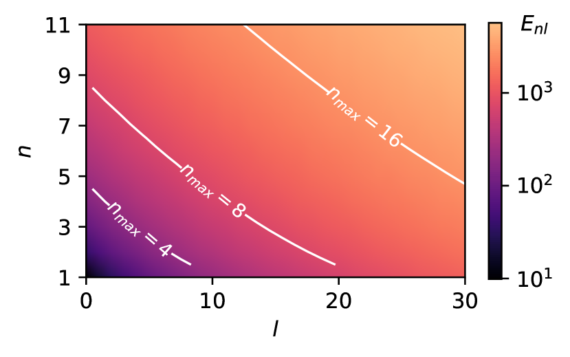
Figure 1: A heat map of the Laplacian eigenvalue $E_{nl}$ in units of $1/a^{2}$, showing the regions of the $n,l$ plane that are included in the LE bases with $E_{\rm max}=E_{n_{\rm max},0}=(n_{\rm max}\pi/a)^{2}$ for $n_{\rm max}$ = 4, 8, and 16.

The connection between small eigenvalues of $-\nabla^{2}$ and smooth eigenfunctions can be understood by considering the Dirichlet problem applied to the 3D sphere. As solutions of the more general Dirichlet problem in a region $\Omega$ of $N$-dimensional real space $\mathbf{x}^{N}$, the eigenstates of $-\nabla^{2}$ have the following property: each successive eigenstate $u(\mathbf{x})$, starting from the one with the lowest eigenvalue, minimises the Rayleigh quotient

$$Q=\left.\displaystyle{\int_{\Omega}\left|\nabla u(\mathbf{x})\right|^{2}\,{\rm d}\mathbf{x}}\middle/\displaystyle{\int_{\Omega}\left|u(\mathbf{x})\right|^{2}\,{\rm d}\mathbf{x}}\right.$$ (10)

subject to the constraint that $u(\mathbf{x})$ is zero on the boundary of $\Omega$ and orthogonal to all eigenstates with smaller eigenvalues. If we take $Q$ as a measure of smoothness, the LE basis truncated via the eigenvalue criterion is thus the smoothest possible basis within the region $\Omega$, which in our case is the 3D sphere, and the eigenvalue $E_{nl}$ quantifies the smoothness of each solution. Truncating the LE basis by retaining the functions with $E_{nl}\leq E_{\rm max}$ is analogous to truncating the spherical harmonic basis by retaining the functions with $l\leq l_{\rm max}$, and it reduces the specification of the basis to a single parameter. The constraint that $E_{nl}\leq E_{\rm max}$ implies that fewer spherical harmonics will be retained in the basis as $n$ increases, so it will contain fewer functions than a direct product basis with the same values of $n_{\rm max}$ and $l_{\rm max}$. This is illustrated in Fig. 1, which shows the regions of the $n,l$ plane that are included in the LE bases with $E_{\rm max}=E_{n_{\rm max}0}$ for various values of $n_{\rm max}$.

II.3 Basis-set smoothness

Smoothness is a desirable feature of machine-learning schemes because it results in a well-behaved interpolation of machine-learned properties to configurations that are not present in the training set. This is an established concept in the atomistic machine learning literature, where smoothness is often enforced through the regularizing effect of including penalty terms in the loss. Smoothing strategies range from the naive Gaussian prior of kernel ridge regression (KRR) to more sophisticated regularization schemes such as that of Ref. 28. The Gaussian smoothing of atomic densities first introduced in SOAP⁵ can also be considered as a regularization. For models involving a basis set representation of the atom density, the regularity of the approximation also depends on the smoothness of the basis functions. Here we intend to show how using a quantifiable smoothness criterion to guide both the choice of the basis set and the truncation of higher-order density correlation features is beneficial to the performance of atomistic ML models.

The Rayleigh quotient in Eq. (10) is clearly just one of many possible measures of the regularity of a function: one could take its mean square curvature, its Lipschitz constant, etc. Perhaps the best way to motivate our choice is to note that the solutions of the Dirichlet problem with periodic boundary conditions are plane waves. The notion that a truncated Fourier expansion is a natural way to enforce regularity is well established, and indeed in plane wave electronic structure codes it is customary to express the basis set truncation in terms of a kinetic energy cutoff. The LE construction yields an analogous basis that is adapted to the symmetry and the boundary conditions of the present problem. This idea has already been exploited in atomistic machine learning: Ref. 15 and the existing DimeNet framework ¹⁴ already use spherical Bessel functions to evaluate radial descriptors, the latter arguing that their bounded maximum frequencies confer both smoothness and stability on the resulting model predictions.

II.4 Unsupervised measures of basis-set quality

We shall now describe three different metrics that can be used to assess the quality of basis sets such as the LE basis introduced in Sec. II.B: a residual variance¹³ metric $\ell_{X}$, a residual Jacobian variance metric $\ell_{J}$, and a Jacobian condition number²⁹ metric $\ell_{CN}$. For the first two of these, it is possible to construct a basis of any desired size that, for a given dataset, is optimal with respect to the metric, and so provides a gold standard against which other bases can be compared. We shall explain how to do this in Sec. II.D. We do not yet know how to construct a finite basis that is optimal for the Jacobian condition number metric, but we do at least know the value that the metric takes in the limit of a complete basis³⁰, so we can use that as the gold standard instead.

II.4.1 Residual variance

Since the expansion in Eq. (1) aims to discretize the $i$-centered neighbor density, a natural criterion for the quality of a basis is how well it minimizes the error in the approximation of $\rho_{i}(\mathbf{x})$. For a given dataset, this can be defined as the normalised $L^{2}$ residual

$$\ell_{X}={\displaystyle{\sum_{i}\int\operatorname{d}{\!\mathbf{x}}\,\,\Bigl{|}\rho_{i}(\mathbf{x})-\sum_{q}c_{q}^{i}\psi_{q}(\mathbf{x})\Bigr{|}^{2}}\over\displaystyle{\sum_{i}\int{\rm d}\mathbf{x}\,\rho_{i}(\mathbf{x})^{2}}},$$ (11)

where $q$ is a shorthand for the $nlm$ basis indices, and $i$ runs over all atomic environments in the dataset. If the discrete basis is orthonormal, then one can compute the numerator in this expression as the difference between the mean $L^{2}$ norm of the neighbor density and the norm of the coefficients $c_{q}^{i}=\innerproduct*{q}{\rho_{i}}$,

$$\ell_{X}={\displaystyle{\sum_{i}\left[\int\operatorname{d}{\!\mathbf{x}}\,\innerproduct*{\mathbf{x}}{\rho_{i}}^{2}-\sum_{q}\innerproduct*{q}{\rho_{i}}^{2}\right]}\over\displaystyle{\sum_{i}\int\operatorname{d}{\!\mathbf{x}}\,\innerproduct*{\mathbf{x}}{\rho_{i}}^{2}}},$$ (12)

or equivalently as the difference between the norm of the coefficients in a complete basis and those in a truncated discretization. The numerator in Eq. (12) is not exactly a difference between two variances, because the density and the coefficients are usually not centered to have zero mean over the data set, but we shall nevertheless call $\ell_{X}$ a residual variance metric following Ref. ¹³.

II.4.2 Residual Jacobian variance

The Jacobian of the features quantifies their sensitivity to atomic displacements. It can be written in terms of the derivatives of the continuous atom density as

$$J_{\mathbf{x},ij\alpha}=\frac{\partial\innerproduct*{\mathbf{x}}{\rho_{i}}}{\partial r_{j\alpha}}\equiv\innerproduct*{\mathbf{x}}{\partial_{j\alpha}\rho_{i}}=\sum_{j^{\prime}}\frac{\partial\innerproduct*{\mathbf{x}}{\mathbf{r}_{j^{\prime}i};g}}{\partial r_{j\alpha}}\\ =-\frac{\partial g(\mathbf{x}-\mathbf{r}_{ji})}{\partial x_{\alpha}}\equiv\innerproduct*{\mathbf{x}}{\mathbf{r}_{ji};\partial_{\alpha}g},\phantom{xxxx.}$$ (13)

where $\alpha$ runs over the Cartesian axes, and in terms of discrete basis states as

$$J_{q,ij\alpha}=\frac{\partial\innerproduct*{q}{\rho_{i}}}{\partial r_{j\alpha}}\equiv\innerproduct*{q}{\partial_{j\alpha}\rho_{i}}=\innerproduct*{q}{\mathbf{r}_{ji};\partial_{\alpha}g}.$$ (14)

The Jacobian arises in the calculation of derivatives of ML models (e.g. forces), and it has been used in the past to assess the quality of atomistic representations – both directly³⁰ and via the sensitivity matrix² $\mathbf{J}_{i}^{T}\mathbf{J}_{i}$. In the present context, it is natural to define a residual Jacobian variance metric $\ell_{J}$ for this purpose by analogy with Eq. (12),

$$\!\!\!\ell_{J}={\displaystyle{\sum_{ij\alpha}\left[\int\operatorname{d}{\!\mathbf{x}}\,\innerproduct*{\mathbf{x}}{\partial_{j\alpha}\rho_{i}}^{2}-\sum_{q}\innerproduct*{q}{\partial_{j\alpha}\rho_{i}}^{2}\right]}\over\displaystyle{\sum_{ij\alpha}\int\operatorname{d}{\!\mathbf{x}}\,\innerproduct*{\mathbf{x}}{\partial_{j\alpha}\rho_{i}}^{2}}},$$ (15)

in which the numerator can again be written equivalently as the difference between the norm of the coefficients $\innerproduct*{q}{\partial_{j\alpha}\rho_{i}}$ in a complete basis and those in a truncated discretization.

II.4.3 Jacobian condition number

We shall base our last metric on the condition number of the Jacobian, that is the ratio between the largest and smallest non-zero singular values of $\mathbf{J}_{i}$. As discussed in Ref. 30, in the limit of a sharp Gaussian smearing $\sigma$ and of a complete basis, all the non-zero singular values of $\mathbf{J}_{i}$ take the same value, because the elements of $\mathbf{J}_{i}^{T}\mathbf{J}_{i}$ become

$$\int\operatorname{d}{\!\mathbf{x}}\,\innerproduct*{\partial_{j\alpha}\rho_{i}}{\mathbf{x}}\innerproduct*{\mathbf{x}}{\partial_{j^{\prime}\alpha^{\prime}}\rho_{i}}=\\ \int\operatorname{d}{\!\mathbf{x}}\,\innerproduct*{\mathbf{r}_{ji};\partial_{\alpha}g}{\mathbf{x}}\innerproduct*{\mathbf{x}}{\mathbf{r}_{j^{\prime}i};\partial_{\alpha^{\prime}}g}\underset{\sigma\rightarrow 0}{\sim}\delta_{\alpha\alpha^{\prime}}\delta_{jj^{\prime}}\frac{\sqrt{\pi}^{3}\sigma}{2},$$ (16)

and so the condition number tends to one. An appropriate Jacobian condition number metric is therefore

$$\ell_{CN}=\frac{1}{n_{\text{train}}}\sum_{i}\frac{s_{\text{max}}(\mathbf{J}_{i})}{s_{\text{min}}(\mathbf{J}_{i})}-1,$$ (17)

where $n_{\text{train}}$ is the number of $i$-centered environments in the training set and $s_{\rm max}(\mathbf{J}_{i})$ and $s_{\rm min}(\mathbf{J}_{i})$ are the largest and smallest non-zero singular values of $\mathbf{J}_{i}$ (the square roots of the largest and smallest eigenvalues of $\mathbf{J}_{i}^{T}\mathbf{J}_{i}$).

From a numerical perspective, condition numbers in the hundreds or thousands are perfectly manageable with floating point arithmetic. However, we would argue that it is beneficial to approach the limit $\ell_{CN}\rightarrow 0$, because this implies that the discretized expansion coefficients are equally sensitive to all types of distortions; i.e., that the basis set does not artificially make the descriptors more sensitive to some deformations than to others. Indeed, it has recently been shown that numerical instabilities that result in moderate values of the Jacobian condition number can affect substantially the performance of ML models^{31; 32}. For the $\ell_{CN}$ metric to be meaningful, there must be at least three times more functions in the basis set than the maximum number of neighbors of any atom $i$ in the data set, so that all the sensitivity matrices $\mathbf{J}_{i}^{T}\mathbf{J}_{i}$ have full rank. Furthermore, the cutoff that is applied in defining the density must be sharp (so that all retained neighbors $j$ of atom $i$ are fully inside the cutoff), and no feature tuning through a radial scaling of the neighbor contributions^{17; 33} can be applied. Incidentally, the fact that the modulating the feature sensitivity in a physically-motivated manner has a significant positive impact on model performance reinforces the notion that it is better to avoid the unpredictable, noisy modulation of the sensitivity that is caused by the choice of a non-smooth basis.

II.5 Metric-optimized bases

The logical next step after having defined metrics to assess the quality of a basis is to look for a construction that yields a basis that is optimal with respect to each metric for a given data set. For the residual variance metric $\ell_{X}$, this step has already been taken in Ref. 13, so here we only sketch the main ideas.

Starting from a basis set expansion in a large set of primitive basis functions $\{\ket{p}\}$, one considers an orthogonal contraction of the expansion coefficients

$$\innerproduct*{q}{\rho_{i}}=\sum_{p}U_{qp}\innerproduct*{p}{\rho_{i}},$$ (18)

in which the orthogonal matrix $\mathbf{U}$ is chosen to diagonalize the real symmetric “covariance” matrix¹³

$$C_{pp^{\prime}}=\sum_{i}\innerproduct*{p}{\rho_{i}}\innerproduct*{\rho_{i}}{p^{\prime}},$$ (19)

such that

$$\sum_{pp^{\prime}}U_{qp}C_{pp^{\prime}}U_{q^{\prime}p^{\prime}}=\gamma_{q}\,\delta_{qq^{\prime}}.$$ (20)

Then since

$$\sum_{iq}\innerproduct*{q}{\rho_{i}}^{2}=\sum_{q}\gamma_{q},$$ (21)

it is clear that the functions $\ket{q}$ with the largest eigenvalues $\gamma_{q}$ provide an optimum contracted basis for the minimization of $\ell_{X}$ in Eq. (12).

Symmetry considerations imply that for a randomly-oriented data set the cross-correlations between features with different SO(3) character must be zero, and so in practice one computes separate blocks of the covariance matrix for each equivariant component

$$C^{\lambda}_{pp^{\prime}}=\sum_{i\mu}\innerproduct*{p}{\overline{\rho_{i}^{\otimes 1};1;\lambda\mu}missing}\innerproduct*{p^{\prime}}{\overline{\rho_{i}^{\otimes 1};1;\lambda\mu}missing}.$$ (22)

As discussed in Ref. 13, it is possible to compute explicitly the radial functions associated with the optimal combinations, and to evaluate the expansion coefficients by approximating them with splines. Since the number of spherical harmonics increases with increasing $\lambda$, we retain the covariance eigenstates with the largest values of $\gamma_{q}/(2\lambda+1)$ so as to achieve the most efficient contraction to a given number of basis functions. Since it gives the optimum value of the metric $\ell_{X}$ for a given dataset, we shall refer to the resulting basis as the X-OPT basis set.

An optimal contracted basis for the Jacobian variance metric $\ell_{J}$ in Eq. (15) can be constructed in the same way, by computing the Jacobian covariance matrix in the primitive basis

$$\!\!\!K^{\lambda}_{pp^{\prime}}\!=\!\sum_{ij\alpha\mu}\innerproduct*{p}{\overline{\partial_{j\alpha}\rho_{i}^{\otimes 1};1;\lambda\mu}missing}\innerproduct*{p^{\prime}}{\overline{\partial_{j\alpha}\rho_{i}^{\otimes 1};1;\lambda\mu}missing},$$ (23)

diagonalizing it, and using the eigenvectors with the largest eigenvalues when weighted by $1/(2\lambda+1)$ to construct the contracted basis functions. We shall refer to the resulting basis as the J-OPT basis set. Both this and the X-OPT basis can be related to the maximization of a Rayleigh quotient akin to Eq. (10), as we discuss in Appendix B and in the SI.

II.6 Higher correlation orders

Our discussion so far has focused on the discretization of the neighbor density, which when expressed using spherical harmonics for the angular part leads to the first-order atom-centered equivariant correlations $\innerproduct*{n}{\overline{\rho_{i}^{\otimes 1};1;\lambda\mu}missing}$. High-accuracy models, however, require higher orders of ACDCs, either built explicitly or through an equivariant network architecture. One should therefore consider how the above ideas generalize to high-order equivariants.

II.6.1 Laplacian eigenstates

The solution of the Laplacian eigenvalue problem in Eq. (7) generates the smoothest possible basis in the 3D sphere $\Omega$. More generally, an analogous Dirichlet problem can be solved in the $\Omega^{\nu}$ hypersphere, where the density $\nu$-correlation $\rho_{i}^{\otimes\nu}$ is defined. The associated Laplacian eigenvalue equation is

$$-\Big{(}\sum_{k=1}^{\nu}\mathbf{\nabla}_{k}^{2}\Big{)}\,\Psi(\{\mathbf{x}_{k}\})=E\,\Psi(\{\mathbf{x}_{k}\}).$$ (24)

Since this is separable into $\nu$ distinct eigenvalue equations, one for each 3D sphere which constitutes the tensor product, the eigenstates are

$$\Psi_{\{n_{k}l_{k}m_{k}\}}(\{\mathbf{x}_{k}\})=\prod_{k=1}^{\nu}\psi_{n_{k}l_{k}m_{k}}(\mathbf{x}_{k}),$$ (25)

and the eigenvalues are

$$E_{\{n_{k}l_{k}\}}=\sum_{k=1}^{\nu}E_{n_{k}l_{k}},$$ (26)

where $\psi_{nlm}(\mathbf{x})$ and $E_{nl}$ are the eigenstates and eigenvalues of Eq. (7). Furthermore, when a tensor product of atomic densities $\rho_{i}^{\otimes\nu}(\{\mathbf{x}_{k}\})$ is expanded in this basis, the resulting integral is also separable, giving

$$\begin{split}\int_{\Omega^{\nu}}\Psi_{\{n_{k}l_{k}m_{k}\}}(\{\mathbf{x}_{k}\})\rho_{i}^{\otimes\nu}(\{\mathbf{x}_{k}\})\,\operatorname{d}{\!\{}\,\mathbf{x}_{k}\}=\phantom{xxxxx}\\ \prod_{k=1}^{\nu}\int_{\Omega}\psi_{n_{k}l_{k}m_{k}}(\mathbf{x}_{k})\rho_{i}(\mathbf{x}_{k})\,\operatorname{d}{\!\mathbf{x}}\,_{k}=\prod_{k=1}^{\nu}c^{i}_{n_{k}l_{k}m_{k}},\end{split}$$ (27)

where the $c^{i}_{nlm}=\innerproduct*{nlm}{\rho_{i}}$ are the equivariant $\rho_{i}^{\otimes 1}$ density expansion coefficients we have considered above.

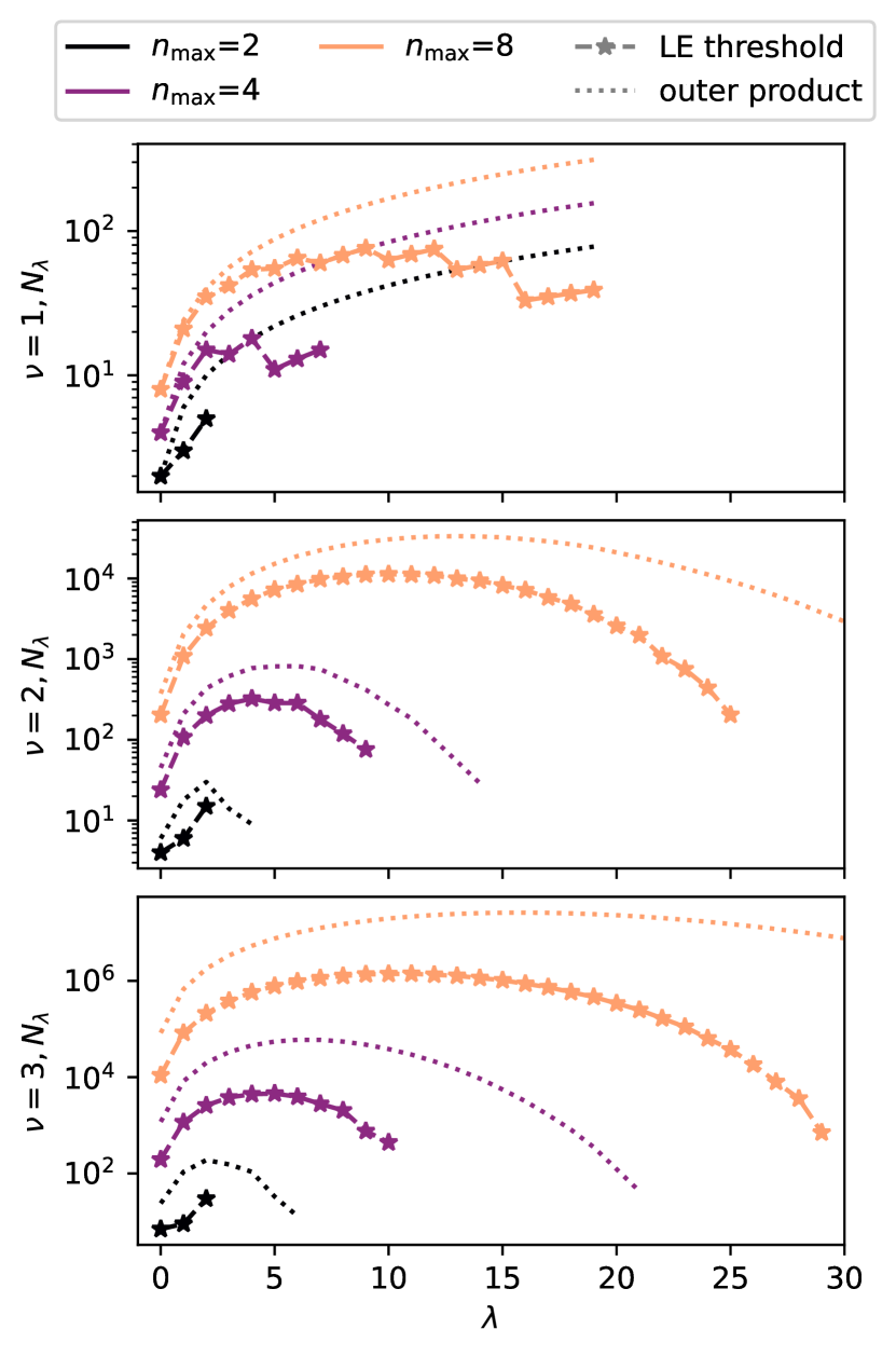
Figure 2: Number of $\innerproduct*{q}{\overline{\rho_{i}^{\otimes\nu};\lambda\mu}missing}$ features retained for each equivariant channel $\lambda$, with (top to bottom) $\nu=1,2,3$. Dashed lines correspond to the features retained by applying the threshold $E_{\rm max}(\nu)=E_{\rm max}(1)+(\nu-1)E_{10}$ at each iteration, with $E_{\rm max}(1)=E_{n_{\rm max},0}$. Dotted lines correspond to taking the outer product density basis for $\nu=1$, and the outer product of the lower-order LE features for $\nu=2,3$.

The product of these separable coefficients is an order-$\nu$ equivariant descriptor in the uncoupled angular momentum basis,

$$\prod_{k=1}^{\nu}c^{i}_{n_{k}l_{k}m_{k}}\equiv\innerproduct*{n_{1}l_{1}m_{1};\ldots n_{\nu}l_{\nu}m_{\nu}}{\rho_{i}^{\otimes\nu}}.$$ (28)

As discussed in Ref. 8, these can be transformed into the irreducible coupled form $\innerproduct*{q}{\overline{\rho_{i}^{\otimes\nu};\sigma;\lambda\mu}missing}$, which can also be constructed iteratively using Eq. (6). Considering the iterative construction, it is easy to see that at each order the coupling combines the projections of degenerate LE functions with the same values of $n$ and $l$, and so the irreducible SO(3) equivariant basis states are also eigenstates of the Laplacian in $\Omega^{\nu}$.

It follows that an ACDC construction based on LE functions will generate the smoothest possible (in the sense of a multi-dimensional generalization of Eq. (10)) equivariant basis in which to expand the $\nu$-neighbor density correlations, provided the expansion is truncated appropriately. In particular, smoothness will be achieved at each order $\nu$ by retaining all equivariants with $\Omega^{\nu}$ Laplacian eigenvalues below some threshold $E_{\rm max}({\nu})$. The $\nu$-independent choice

$$E_{\rm max}(\nu)=E_{\rm max}(1)+(\nu-1)E_{10}$$ (29)

is especially convenient because it ensures that every LE basis function with $E_{nl}\leq E_{\rm max}(1)$ is included in at least one $\nu$-neighbor equivariant, and that no LE basis function with $E_{nl}>E_{\rm max}(1)$ is ever used.

Fig. 2 shows that the application of this threshold at each iteration reduces by at least an order of magnitude the number of equivariants relative to the number obtained by computing all possible combinations of the $\nu=1$ features with $E_{nl}\leq E_{\rm max}(1)$. An additional reduction in the number of features can be achieved by applying selection rules that discard linearly dependent terms, such as considering only lexicographically-sorted $(n,l)$ terms⁸. However, this still does not eliminate the exponential scaling of the number of features with $\nu$. An increasingly aggressive truncation might therefore be preferable for larger $\nu$, especially in situations where higher body-order terms are only expected to make a small contribution to the structure-property relations that are the goal of the calculation.

II.6.2 Residual variance

The selection of high-$\nu$ equivariants on the basis of their $\Omega^{\nu}$ Laplacian eigenvalues is clearly only a viable option for the LE basis: it cannot be done for the metric-optimized X-OPT and J-OPT basis sets introduced in Sec. II.D. There are, however, alternative ways to select the high-$\nu$ features for these basis sets,^{8; 34; 35} as we shall now briefly describe for the case of the X-OPT (minimal residual variance) basis.

The basic idea is to retain as much variance as possible in the high-$\nu$ density expansion coefficients, just as the X-OPT basis retains maximum variance in the $\nu=1$ coefficients. The limit on the amount of variance that can be retained with a finite basis is determined by the CG iteration in Eq. (6), which implies that the square modulus of each combination of features is the product of the square moduli of the lower-order features being combined:¹³

$$\sum_{l_{1}l_{2}}\sum_{\sigma\lambda\mu}\left|\innerproduct*{ql_{2};nl_{1}}{\overline{\rho_{i}^{\otimes{\nu+1}};\sigma;\lambda\mu}missing}\right|^{2}=\\ \sum_{l_{1}m_{1}}\left|\innerproduct*{n}{\overline{\rho_{i}^{\otimes 1};1;l_{1}m_{1}}missing}\right|^{2}\sum_{\sigma_{2}l_{2}m_{2}}\left|\innerproduct*{q}{\overline{\rho_{i}^{\otimes\nu};\sigma_{2};l_{2}m_{2}}missing}\right|^{2}.$$ (30)

Clearly, therefore, the fraction of the variance that can be retained in the high-$\nu$ equivariants of a finite $nlm$ basis decreases exponentially with increasing $\nu$. The goal is nevertheless to retain as much of this limiting variance as possible, while at the same mitigating the exponential increase in the number of equivariants with $\nu$.

The $N$-body iterative contraction of equivariants (NICE) scheme⁸ does this by performing a principal component analysis (PCA), and then evaluating the combinations with the highest variance so as to yield the optimal features for a given size of the pool of ACDC equivariants. However, this a posteriori contraction scheme requires the evaluation of a large number of features before applying the projection step, which can become quite expensive. We have therefore also tested a cheaper iterative variance optimization (IVO) scheme that pre-selects a smaller number of high-order features and functions in a similar way to the iterative CUR selection of Refs. 34; 35. This IVO scheme is described in Appendix C and its high-$\nu$ equivariants are compared with those of the PCA scheme for the X-OPT basis in our benchmark calculations in Sec. III.

II.6.3 Jacobian condition number

Consider the Jacobian ${\bf J}_{i}$ computed for an equivariant of body order $\nu$, with elements $J_{q\sigma\lambda\mu,ij\alpha}=\innerproduct*{q}{\overline{\partial_{j\alpha}\rho_{i}^{\otimes\nu};\sigma;\lambda\mu}missing}$. As we show in Appendix D, in the sharp Gaussian smoothing and complete basis set limit, $\mathbf{J}_{i}^{T}\mathbf{J}_{i}$ can be evaluated in closed form, yielding

$$\!\!\!\sum_{q\sigma\lambda\mu}\innerproduct*{q}{\overline{\partial_{j\alpha}\rho_{i}^{\otimes\nu};\sigma;\lambda\mu}missing}\innerproduct*{q}{\overline{\partial_{j^{\prime}\alpha^{\prime}}\rho_{i}^{\otimes\nu};\sigma;\lambda\mu}missing}=k_{i}\delta_{jj^{\prime}}\delta_{\alpha\alpha^{\prime}},$$ (31)

which again implies a condition number of one. [Note that this expression involves summing over multiple equivariant channels, and that in general invariant features cannot have uniform sensitivity: for high-symmetry structures (and some non-symmetric ones, in the case of degenerate low-order descriptors) $\innerproduct*{q}{\overline{\partial_{j\alpha}\rho_{i}^{\otimes\nu};1;00}missing}$ is strictly singular.³⁰]

III Benchmarks

We shall now compare the performance of the LE basis with that of the data-driven X-OPT and J-OPT bases and the Gaussian-type orbital (GTO) basis presented in Ref. 11. To do this we shall use the three metrics introduced in Section II.4, as well as regression exercises involving DFT potential energies as the supervised target.

III.1 Chemical datasets and parameters

We have performed benchmark calculations on the AIRSS ³⁶ carbon dataset ³⁷ and the random methane dataset³⁸ (using carbon-centered environments only). The random selection of carbon-centered environments in the methane dataset provides a highly uniform distribution of neighbors, whereas the AIRSS carbon structures are more representative of the sort of systems for which potential energies are typically learned. A subset of the 10,000 lowest-energy structures in the random methane dataset was also employed to illustrate how a data-driven basis can be optimized for predominantly tetrahedral structures. A tetrahedral order parameter³⁹ is used in the SI to establish the tetrahedral character of the low-energy methane structures.

The cutoff radius ${r_{\text{cut}}}$ was set to $3.5$ Å for the random and low-energy methane datasets, and to $5.0$ Å for the condensed phase carbon dataset so as to include more coordination shells. Gaussian-smoothed densities were used, with a Gaussian smoothing parameter of $\sigma=0.2$ Å. Since all the C-H distances in the methane dataset are below $r_{\rm max}=3$ Å, the hydrogen density with this smoothing parameter is essentially zero at $r_{\rm cut}=3.5$ Å, so we used a radius of $a=r_{\rm cut}$ when defining the LE basis functions. For the learning exercises on the condensed phase carbon dataset, we also used $a=r_{\rm cut}$, but introduced a cutoff function to damp the density to zero at this radius. The precise form of the cutoff function is given along with the other details of the LE expansion in Appendix A.

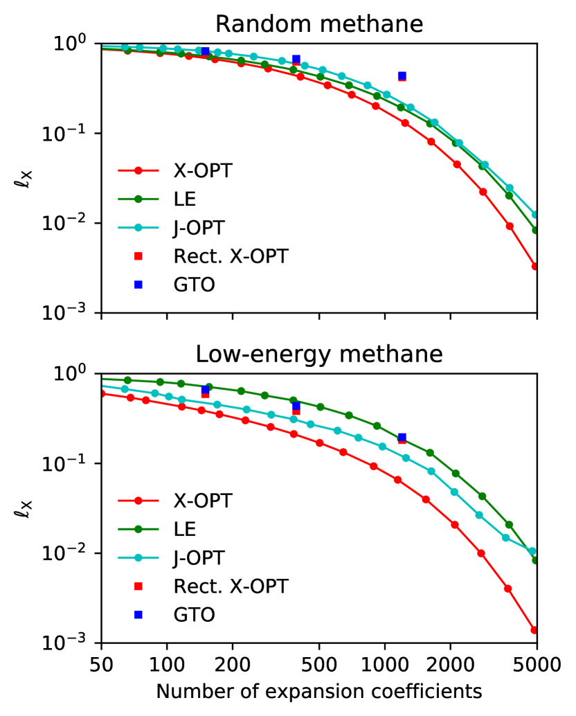
Figure 3: Residual variances of different bases on methane structures. $\ell_{X}$ is the normalised $L^{2}$ error in the approximation to the Gaussian-smoothed density in Eq. 12. The curves are the results obtained with the X-OPT, LE, and J-OPT basis sets truncated to the specified number of $(n,l)$ basis functions (or expansion coefficients) as described in the text. The square markers correspond to full outer-product X-OPT and GTO basis sets with $(n_{\text{max}},l_{\text{max}})=(6,4),(8,6)$ and (12,9).

The LE expansion was truncated by retaining basis functions with $E_{nl}\leq E_{\rm max}$ as described in Sec. II.B. The more traditional GTO and “rectangular” X-OPT bases, which correspond to using rectangular cutoffs in Fig. 1, were truncated via three representative $(n_{\rm max},l_{\rm max})$ combinations (small $(6,4)$, medium $(8,6)$, and large $(12,9)$), and they are indicated by square markers in our figures.

In what follows we report only selected results that highlight the most important observations for each type of benchmark. A more comprehensive series of plots, together with a more detailed discussion, can be found in the SI.

III.2 Density expansion coefficients

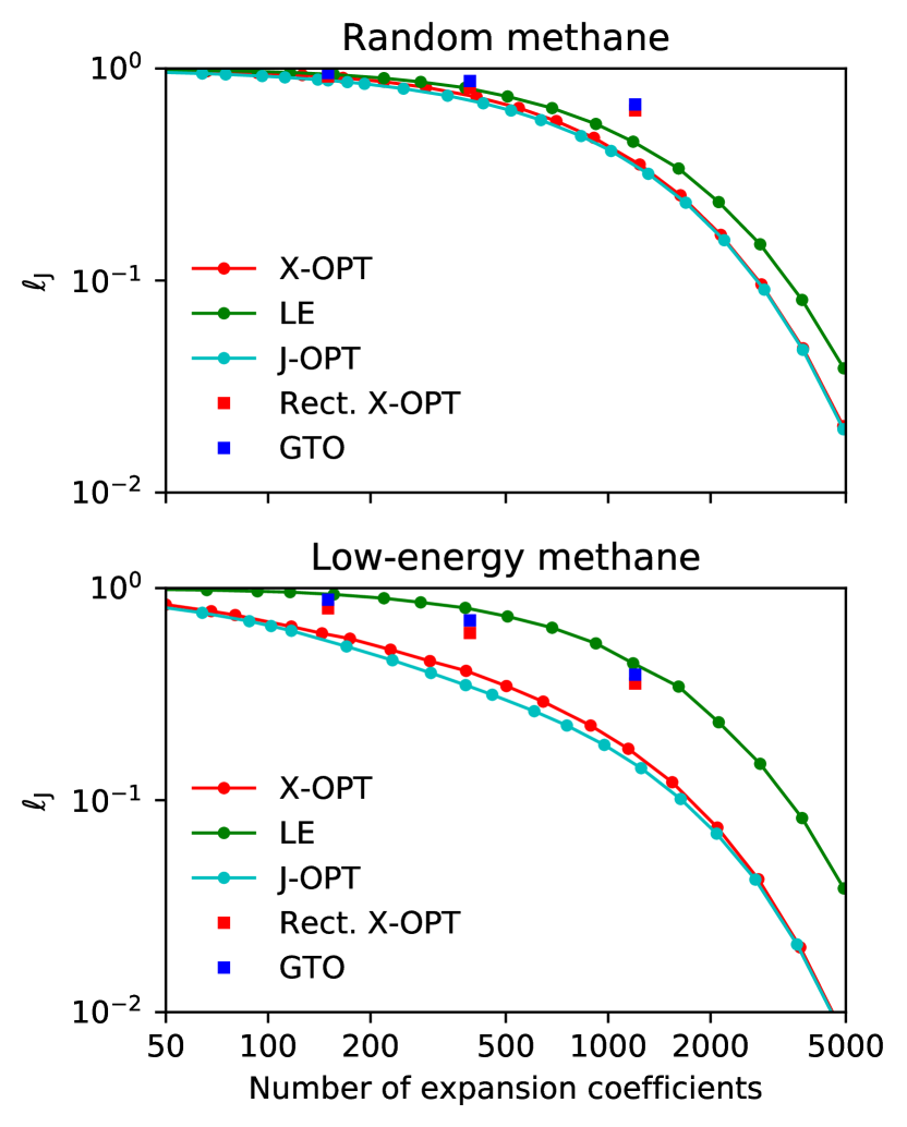
Figure 4: Residual Jacobian variances of different bases on methane structures. $\ell_{J}$ is the error in approximation to the Jacobian of the density expansion defined in Eq. 15. The basis sets are the same as those in Fig. 3.

III.2.1 Residual variance

The residual variance tests conducted on methane are shown in Fig. 3. The X-OPT basis (unsurprisingly) performs best for this metric, while the rectangular bases generally suffer from the exclusion of high-$l$ channels. The LE basis is competitive with all the others, and, given an X-OPT basis of a certain size, it only takes a slightly larger LE basis to match it in terms of captured variance. The benefits of using a data-driven basis are more pronounced for the low-energy methane configurations, in which the H atoms are non-uniformly distributed around the central carbon.

III.2.2 Jacobian variance

The Jacobian variance tests for methane shown in Fig. 4 confirm that the J-OPT basis is optimum for this alternative metric. Once again, the $(n_{\rm max},l_{\rm max})$-truncated bases suffer from the lack of high-$l$ coefficients. The LE basis is competitive with the data-adapted bases for random methane, although noticeably less so for the heavily optimizable low-energy methane structures.

Comparing Figs. 3 and 4 reveals the trade-off between optimizing the variance and the Jacobian variance: although one has to choose one target property to optimize, the resulting basis set also performs well for the other task. This is especially true of the X-OPT basis, which does remarkably well on the Jacobian variance test. Another key observation is that tuning the number of radial functions within each $l$ channel results in a systematically more efficient encoding of information than is present in an outer-product basis of comparable size. This is particularly evident when comparing the two truncation methods for the X-OPT basis. When using the same number of radial functions for each angular momentum channel, the improvement over a primitve GTO basis is barely noticeable, whereas using an adaptive truncation of the radial basis yields an improvement of a factor between 2 and 5 in both $\ell_{X}$ and $\ell_{J}$.

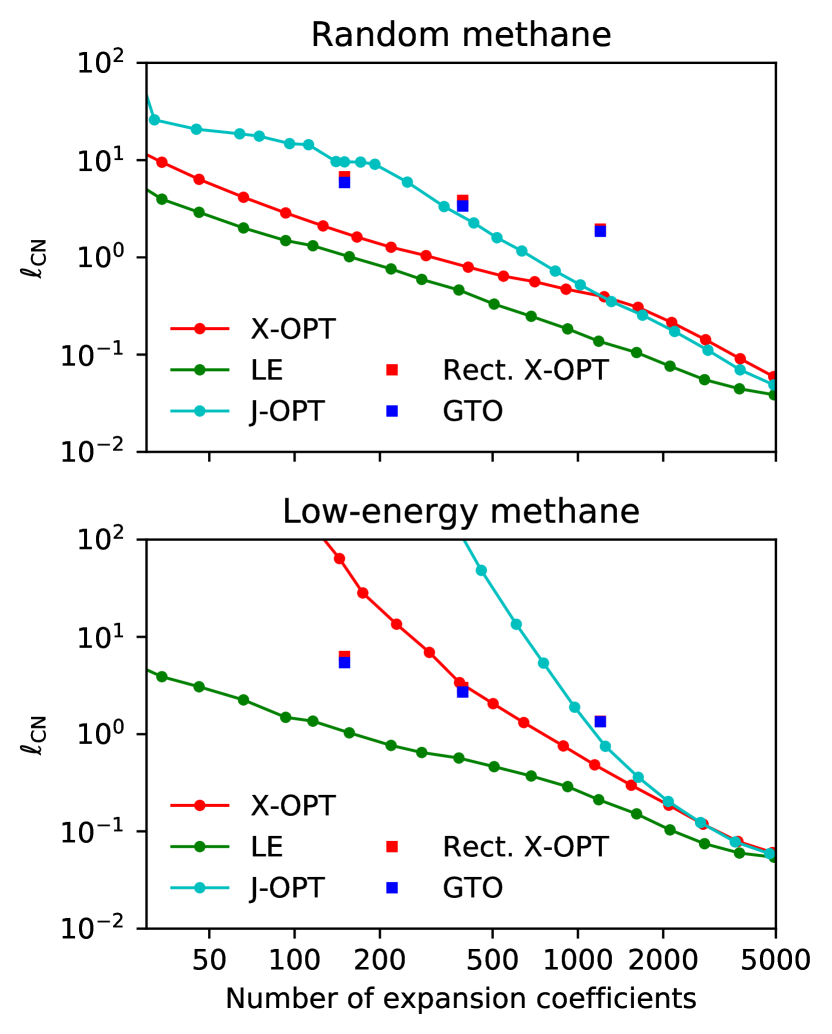
Figure 5: Jacobian condition number tests on methane structures. $\ell_{\text{CN}}\rightarrow 0$ indicates that the condition number of the density-expansion Jacobian tends to one. The basis sets are the same as those in Fig. 3.

III.2.3 Jacobian condition number

The Jacobian condition number (CN) tests are shown in Fig. 5. In contrast to the variance and Jacobian variance tests, these CN tests show the LE basis outperforming all of the other basis sets we have considered. Because it is smooth in the entire atomic neighborhood, even a small LE basis yields a uniform approximation to the atom density, and therefore small anisotropy in the sensitivity of the features to structural deformations, even though it provides a worse $L^{2}$ approximation to the Jacobian (see Fig. 4). The X-OPT basis has a comparable CN to the LE basis for the random methane data set, but a much higher CN for the more optimizable low-energy methane subset. This behaviour can be understood by noting that adapting the basis to the data set makes it less uniform, leading to a more anisotropic response to deformations. A similar reasoning explains why the J-OPT basis, which provides a better approximation to the density derivatives, yields an even higher CN (and therefore a worse result still in this respect) than the X-OPT basis.

III.3 Equivariant $\nu=2$ features

The density expansion coefficients ($\nu=1$ equivariant features) are the starting point of all density-correlation descriptors. In order to build accurate ML models, however, it is almost mandatory to increase the correlation order beyond $\nu=1$. To investigate the impact of the body-order iteration on the different metrics we have introduced, we have repeated the residual variance and Jacobian condition number tests using $\nu=2$ equivariants. For this we have confined our attention to the LE and X-OPT bases, because they perform well on the other tests and their associated truncation criteria readily generalize to higher body-order features.

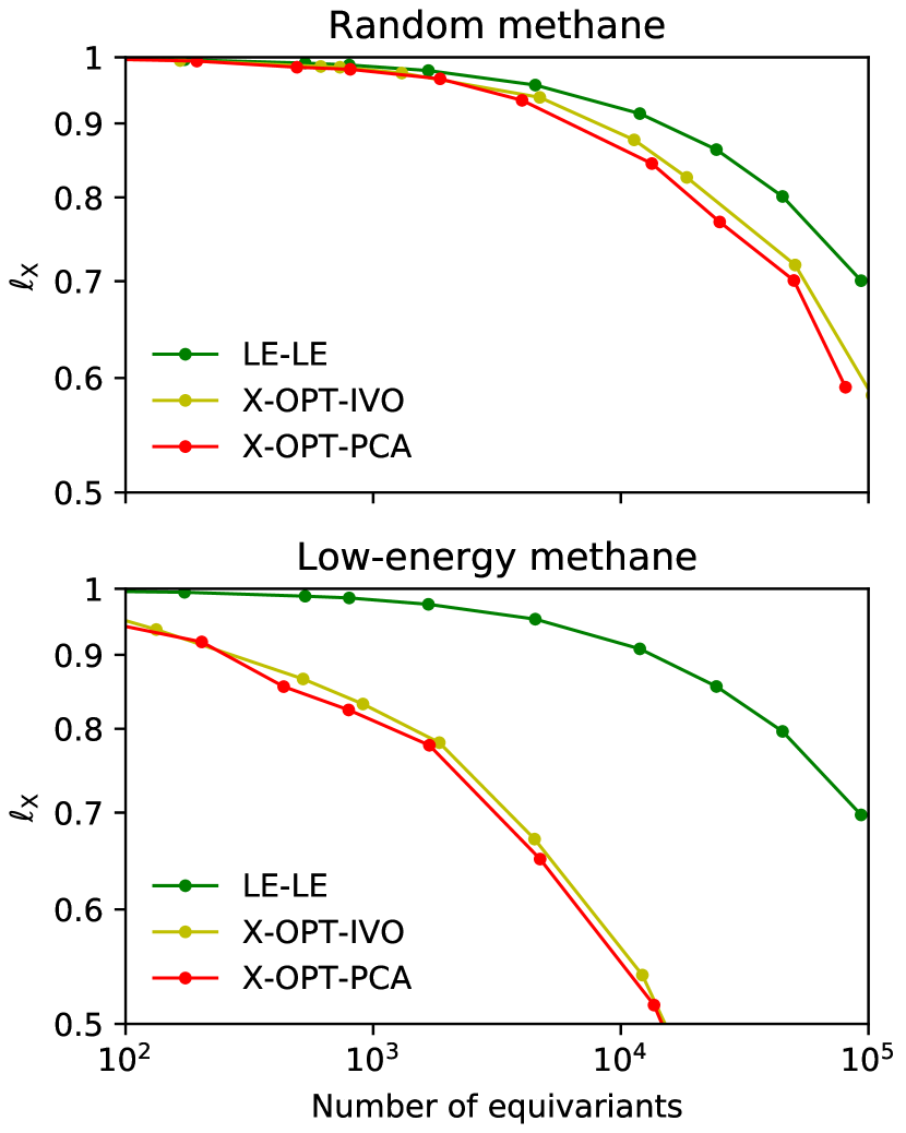
Figure 6: Residual variances of $\nu=2$ equivariants on methane structures. The LE-LE data corresponds to density correlations built on the LE basis, and truncated based on the LE eigenvalues. The X-OPT-PCA and X-OPT-IVO data correspond to a variance-optimal density expansion, with correlations further contracted using PCA or selected using the IVO scheme.

III.3.1 Residual Variance

The residual variances of the LE and X-OPT $\nu=2$ equivariant features for the random and low-energy methane structures are shown in Fig. 6. The PCA contraction retains more variance than the LE truncation, as is obvious from its construction. Contrary to the $\nu=1$ case, however, the retained variance gap is large, especially for the low-energy methane structures, indicating that the $\nu=2$ equivariants are significantly more compressible than the $\nu=1$ density expansion coefficients.

From a numerical point of view, this comparison is not entirely fair, because while the X-OPT basis can be evaluated at no additional cost¹³ compared to the LE basis, the PCA contraction of higher-order representations requires the evaluation of all features before contracting them. This makes it more expensive than using Eq. (29) to pre-select the relevant higher-order equivariant features for the LE basis, as we have done in computing the LE-LE curves in Fig. 6. The IVO scheme, which is based on the selection of the highest variance features, is more closely comparable: after having identified the optimal components, it only requires evaluating those that have been chosen. The resulting IVO equivariants in Fig. 6 have slightly higher residual variance than those from PCA, but they are still significantly lower than those from LE-LE.

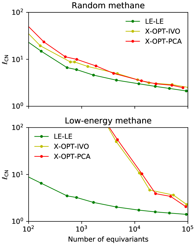
Figure 7: $\nu=2$ Jacobian condition number tests on methane structures. The LE-LE, X-OPT-PCA, and X-OPT-IVO expansions of the $\nu=2$ equivariants are the same as in the residual variance tests in Fig. 6.

III.3.2 Jacobian condition number

The Jacobian condition numbers of the $\nu=2$ equivariants from the X-OPT and LE methods are shown in Fig. 7. As in the $\nu=1$ case, the LE equivariants give the smallest CN, for both the random and the low-energy methane structures. The CN of the X-OPT equivariants increases significantly on going from the random to the low-energy structures, regardless of the feature reduction method employed (PCA contraction or IVO selection). This reinforces the notion that adapting the basis to focus on the correlations that are most common in a given data set increases – rather than decreases – the anisotropy of the Jacobian, at least in the small basis set limit. As more $\nu=2$ equivariants are included in the X-OPT calculation, the Jacobian CN decreases, and by the time there are 10⁵ it appears to be approaching that of the LE calculation.

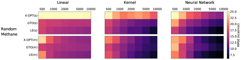
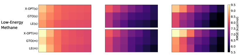
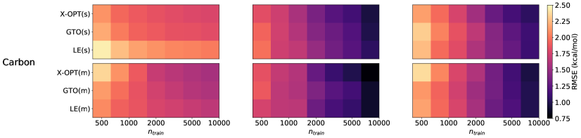
Figure 8: Learning using invariants with $\nu\leq 2$. (s) denotes a small basis, and (m) denotes a medium-sized basis. Each of these is constructed so as to contain a similar number of basis functions for all three methods (X-OPT, GTO, and LE), as described in the SI. Larger expansion coefficient sets exhibit significant overfitting in the case of methane (for these relatively small training set sizes), and they do not significantly improve on their medium-sized counterparts in the case of carbon (see the SI). Additional results for the J-OPT and rectangular X-OPT bases are also available in the SI.

III.4 Learning from invariant features

While the metrics discussed above provide an “unsupervised” estimate of the quality of the basis set used for the density expansion, the ultimate goal of most ML models is to achieve accurate predictions for a target property. We take as a paradigmatic example the construction of models of the interatomic potential, using only energies for training, comparing the performance of the different radial basis sets we have considered. As in the previous section, we show results for some representative cases, and refer the reader to the SI for further examples and a more comprehensive discussion.

III.4.1 Invariants with $\nu\leq 2$

Fig. 8 compares the performance of (up to) $\nu=2$ invariants built from different bases as inputs to linear, kernel, and neural network (NN) models. Linear-based learning saturates quickly due to its inability to account for high body-order interactions, while kernel and NN-based models do not suffer from this issue. The relative performance of different bases is similar across different machine learning models, highlighting a high degree of “orthogonality” between the choice of basis and that of the fitting model, at least for the datasets we have considered.

There is comparatively little to choose between the X-OPT, GTO, and LE results in Fig. 8 for either methane dataset – random methane or low-energy methane – regardless of whether the potential is learned from a linear fit, with a non-linear kernel, or with a neural network. The only real outlier is the small X-OPT basis, which performs particularly poorly for the random methane dataset. The “optimization” of this basis to fit the density more accurately than a LE basis of comparable size clearly does not help with this learning exercise. Indeed, while the differences are often small, the LE results are slightly better than those of the other two basis sets in all 12 of the methane panels in Fig. 8.

The results of the carbon tests in Fig.  8 are another matter. This is a simpler problem that can be solved to “chemical accuracy” (a root mean square error of less than 1 kcal/mol) using any of the three basis sets, provided either a non-linear kernel or a neural network is used to extract higher body-order contributions from the invariant features with $\nu\leq 2$. Once this is done, the results for all three basis sets are essentially the same, provided an appropriate cutoff function is applied to the density to make it go smoothly to zero at $r_{\rm cut}$. [As we have done in these tests: for the LE basis, we used the cutoff functions $f_{1}(x)$ and $f_{2}(r_{ij})$ defined in Appendix A. These were also used when constructing the primitive LE basis that was contracted to produce the X-OPT basis functions. For the GTO basis, $f_{1}(x)$ is not needed, so we simply used $f_{2}(r_{ij})$.]

The use of an aggressive cutoff function that emphasizes the short-range interactions, that are dominant for this problem, is essential to achieve the good performance seen in Fig. 8. As has been noted previously^{17; 33; 7}, this type of feature engineering, which incorporates prior knowledge on the target function, is very effective in improving the performance of a ML model. On the other hand, it appears that in this case the choice of basis set plays only a very limited role. The most accurate results for the carbon dataset in Fig. 8 are seen for the X-OPT basis, which is optimized to fit the radially-weighted density once the cutoff function has been introduced. However, these results are only marginally better than those obtained with the LE basis, which is not optimized to fit the dataset at all.

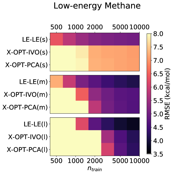
Figure 9: Learning from up to $\nu=3$ invariants. LE-LE denotes a LE basis combined with a Laplacian eigenvalue selection at the $\nu=2$ equivariant level. Similarly, X-OPT-IVO indicates an X-OPT basis ($\nu=1$) and an IVO contraction ($\nu=2$), and X-OPT-PCA indicates PCA contractions at both $\nu=1$ and $\nu=2$. (s), (m), and (l) denote small-sized, medium-sized, and large $\nu=3$ invariant sets, respectively.

III.4.2 Invariants with $\nu\leq 3$.

Given the saturation of the linear learning curves in Fig. 8, the linear learning exercises for the methane datasets were repeated using (up to) $\nu=3$ invariants. The results of these tests are shown in Fig. 9, where it is clear that, when enough $\nu=3$ invariants are included, the curves do not saturate within the range of training set sizes considered. Note also that the use of the LE basis, together with the LE selection scheme for high-order equivariants (LE-LE), affords the lowest RMSEs in these tests for both methane datasets, by a substantial margin. This suggests that the optimum smoothness of the LE basis, which extends in a natural way to the smoothness of the higher body-order features obtained from the LE-LE scheme as described in Sec. II.E, is an important ingredient to successfully learn potential energies from high-$\nu$ invariants. Since this seems to be the direction of travel of much of the most recent work on machine learning potentials,^{3; 7; 8} it could well be the most significant result in this paper, especially since the data-driven and ostensibly “optimized” X-OPT-IVO and X-OPT-PCA results in Fig. 9 are so poor by comparison.

It is important to keep in mind here, though, that the methane dataset, particularly when learning with only C-centered descriptors, is particularly challenging, and heavily dependent on the convergence and resolution of the basis set. Even though the advantage of the LE-LE scheme for other regression tasks, such as learning with both C- and H-centered descriptors, are not be quite so pronounced, they are nonetheless significant (see the next Section, and especially Fig. 10). In particular, it is remarkable that a smoothness criterion, that leads to a very high loss of information content in terms of $\ell_{X}$ (see Fig. 6), proves so effective when it comes to regression performance. This suggests that a complete description of the $\nu$-order density correlations might not be necessary to converge ML models based on them, and that actually seeking the most complete description possible (as is done in X-OPT-PCA) might not be the best approach after all.

III.4.3 Application to body-ordered expansions

The LE-LE idea presented in the previous section is easily extensible to body-ordered expansion frameworks^{7; 8}. We will now show how the LE basis improves over previous basis functions when fitting interatomic potentials for the molecules in the rMD17 dataset.⁴⁰ Given that we will aim to compare with existing results based on the ACE scheme,⁴¹ we will incorporate some of the heuristics that have been used in previous ACE work. Thus, we refer to the resulting model as LE-ACE.

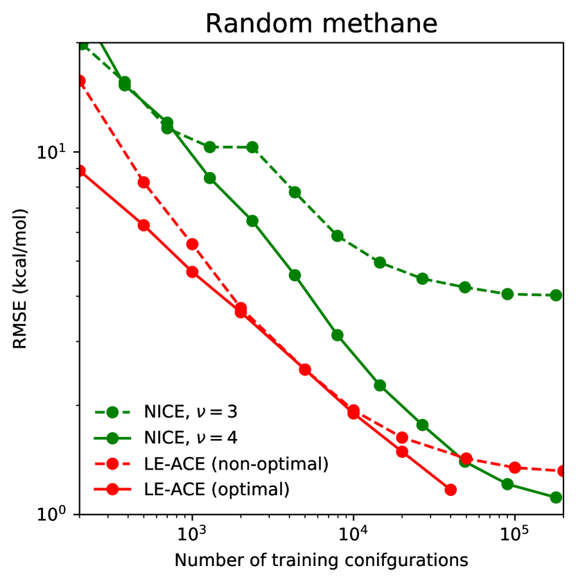
Figure 10: Performance of the LE-ACE model on the random methane dataset. The NICE curves are from Ref. 8. The optimal truncation of LE-ACE follows the $E_{\textrm{max}}{(\nu)}\propto n_{\textrm{train}}^{2/3\nu}$ scaling, while the non-optimal truncation uses the optimal values $E_{\rm max}(\nu)$ for 5000 training structures and extends them to all other points on the learning curve.

Before proceeding to this comparison, we note that one of the challenges when benchmarking linear models is that validation errors depend strongly on regularization, and in particular they depend in a non-monotonic way on the size of the feature vector. For example, when using a small training set one often observes that aggressive truncation results in more transferable models. In the LE-LE context, this means that the $E_{\textrm{max}}{(\nu)}$ values should be optimized as a function of $n_{\textrm{train}}$. This follows because the maximum frequency component of the learned potential at each body order depends on $E_{\rm max}(\nu)$. As more samples are included in the training set, the configuration space of the system is sampled more densely, and therefore higher-frequency components of the potential can be learned. Including basis functions whose frequency is too high leads to overfitting, whereas if $E_{\textrm{max}}{(\nu)}$ is smaller than optimal there will be underfitting.

In order to estimate how $E_{\textrm{max}}(\nu)$ should vary as a function of $n_{\textrm{train}}$, we note that $E_{\textrm{max}}{(\nu)}$ is proportional to the square of the maximum sampled frequency $\omega$ in the $\Omega^{\nu}$ hypersphere. Since $\omega$ is proportional to the inverse of the typical distance $d$ between configurations in the $\Omega^{\nu}$ space, we have $E_{\textrm{max}}{(\nu)}\propto\omega^{2}\propto 1/d^{2}$. If we consider one training point to represent one point in the $\Omega^{\nu}$ hypersphere, the typical distance $d$ scales as $(V^{\nu}/n_{\mathrm{train}})^{1/3\nu}$, where $V^{\nu}$ is the volume of $\Omega^{\nu}$. Hence, $E_{\textrm{max}}{(\nu)}\propto n_{\mathrm{train}}^{2/3\nu}$.

We can illustrate this idea for the random methane dataset by extending the training set beyond the 10,000 configurations we have used in most of the present work. As shown in Fig. 10, the proposed scaling of $E_{\textrm{max}}{(\nu)}$ gives rise to a learning curve that decays linearly on a log-log scale. In contrast, all other learning curves are non-optimal. The $\nu=3$ NICE curve⁸ shows limited accuracy and saturation due to its inability to describe 5-body interactions in the gas-phase methane molecules. The $\nu=4$ NICE and non-optimal LE-ACE curves show signs of saturation (underfitting) in the data-rich regime, as well as overfitting in the data-poor regime, due to their sub-optimal resolution. By contrast, the newly proposed $E_{\textrm{max}}{(\nu)}\propto n_{\mathrm{train}}^{2/3\nu}$ truncation provides a good fit regardless of the amount of training data, suggesting that our frequency-based argument provides a valid heuristic to adapt the resolution of a linear model to the amount of data available.

We will now compare the performance of this new model with that of a standard ACE implementation on the rMD17 dataset⁴⁰, which is widely used as a benchmark, and allows us to compare LE-ACE with several recently-proposed models. This is however a somewhat problematic data set, as it contains highly-correlated structures generated from short, low-temperature molecular dynamics trajectories: as noted in Ref. 42, the most instructive comparisons can be obtained in the data-poor regime. Further details regarding our implementation and additional benchmarks are provided in Appendix E and Section 4 of the SI. We should emphasize here that, for fairness of comparison, we have incorporated a heuristic optimization in the form of a non-linear transformation of the radial coordinate [see Eq. 53], as is almost universally done when learning interactomic potentials in ACE ^{7; 41; 12}.

Molecule	Target	ACE	LE-ACE	NequIP	MACE
Aspirin	E	26.2	22.4(2.0)	19.5	17.0
	F	63.8	59.1(1.3)	52.0	43.9
Azobenzene	E	9.0	9.9(8)	6.0	5.4
	F	28.8	27.5(6)	20.0	17.7
Benzene	E	0.2	0.135(9)	0.6	0.7
	F	2.7	1.44(3)	2.9	2.7
Ethanol	E	8.6	6.6(6)	8.7	6.7
	F	43.0	32.0(1.5)	40.2	32.6
Malonaldehyde	E	12.8	11.3(1.9)	12.7	10.0
	F	63.5	50.9(3.6)	52.5	43.3
Naphthalene	E	3.8	2.9(1)	2.1	2.1
	F	19.7	13.9(3)	10.0	9.2
Paracetamol	E	13.6	14.3(1.8)	14.3	9.7
	F	45.7	45.1(1.6)	39.7	31.5
Salicylic acid	E	8.9	8.3(4)	8.0	6.5
	F	41.7	36.7(1.4)	35.0	28.4
Toluene	E	5.3	4.1(3)	3.3	3.1
	F	27.1	18.4(4)	15.1	12.1
Uracil	E	6.5	5.7(4)	7.3	4.4
	F	36.2	30.7(1.3)	40.1	25.9

Table 1: Benchmark results on the rMD17 dataset⁴⁰, in the smaller and more challenging version presented in Ref. 42, where the training set consists of only 50 structures. The table contains the mean absolute errors of energies (E) and force components (F) in units of meV and meV/Å, respectively, as obtained using ACE [Ref. 41], LE-ACE [Present Work], NequIP [Ref. 24] and MACE [Ref. 42]. The numbers in parentheses after the LE-ACE results are statistical errors in the final digit(s), which represent the standard deviation of five different train/test splits (see SI). The best results for each target are marked in bold.

Our LE-ACE results for the rMD17 dataset are shown in Table I, where they are compared with the results of a standard ACE implementation⁴¹ and those of two state-of-the-art equivariant message-passing neural networks (NequIP²⁴ and MACE⁴²). While there might be other minor differences between the two implementations, it can be seen that the use of the LE basis allows for a significant and systematic improvement in accuracy over the basis functions used in ACE. In some cases, the LE-ACE model is also competitive with NequIP and MACE. It is reasonable to assume that the incorporation of the ideas that underlie the LE basis into NequIP and MACE would lead to similar improvements in the message-passing context to the improvements LE-ACE offers over ACE.

IV Conclusions

In this paper we have investigated the use of the LE basis for the expansion of local atomic densities, explained why this basis, when truncated with the eigenvalue criterion $E_{nl}\leq E_{\rm max}$, provides the smoothest possible basis of a given size within a sphere $\Omega$ in the sense of minimising the Rayleigh quotient in Eq. 10, and described how this property extends in a natural way to the representation of density correlations of arbitrary order $\nu$ within the relevant hyperspheres $\Omega^{\nu}$. Several of these developments have precedents in the recent atomistic machine learning literature. For example, the truncation criterion $E_{nl}\leq E_{\rm max}$ leads to the retention of different numbers of radial basis functions in each angular momentum channel $l$, as is increasingly done when using atomic cluster expansion (ACE) descriptors.^{43; 12} The key difference is that the $E_{nl}\leq E_{\rm max}$ criterion tells us exactly how many radial basis functions to retain for each value of $l$, without the need to introduce any further parameters. We have also described how an analogous criterion can be used to truncate higher body-order features of the LE basis [see Eq. 29], and provided a scaling argument that shows how to adapt the parameters in this more general truncation scheme to the training set size [$E_{\rm max}(\nu)\propto n_{\rm train}^{2/3\nu}$ – see Sec. III.D.3].

We began by arguing that a smooth basis is desirable for machine learning because it implies a smooth interpolation (and possibly extrapolation) of machine-learned properties to configurations that are not present in the training set. Our learning results in Figs. 8– 10 certainly support this argument. In all cases, the LE basis gives results are either comparable to or better than those obtained with data-driven basis sets obtained by optimizing the $L^{2}$ fit to the density, which we find results in a less uniform sensitivity of the density coefficients to atomic displacements.

The advantage of the LE basis is especially apparent in the learning results in Fig. 9, in which the $\nu\leq 3$ invariants are built from $\nu\leq 2$ equivariants that benefit from the smoothness of the LE representation of the density correlations in $\Omega^{2}$. The fact that this advantage is obtained when the LE $\nu=2$ equivariants only capture a small fraction of the variance in the $\nu=2$ density correlations present in the dataset (Fig. 6) is especially interesting, as it suggests that a high resolution representation of the density correlations may not be needed to learn the potential energy.

Our learning results are anti-correlated with the results of our residual variance ($\ell_{X}$) tests in Figs. 3 and 6, but well correlated with the results of our Jacobian condition number ($\ell_{CN}$) tests in Figs. 5 and 7. While this does not imply that the Jacobian condition number is the ultimate indicator of basis set quality, we do believe that it points at the importance of achieving a discretization of the density that has “uniform resolution”, and thereby does not artificially distort the sensitivity of the features to atomic deformations.

A “signal-processing” view, in which features need to provide a basis that fully describes the density correlations, implies an exponential increase in the number of features with body order $\nu$. If instead it suffices to retain enough features to guarantee that the Jacobian is full rank and well-conditioned for every configuration, then one may hope that a number of features proportional to the maximum number of neighbours within $r_{\text{cut}}$ would suffice. Our learning results in Figs. 8–10 suggest that, when it comes to building interatomic potentials, a basis and a truncation strategy that are optimal in a signal-processing sense are less effective than a basis and a truncation strategy aiming for “optimal smoothness”, which is the approach we have taken in this paper.

SUPPLEMENTAL INFORMATION

See supplemental information for a more comprehensive set of benchmarks, its analysis, and a detailed account of the Rayleigh-quotient formulation of optimized bases.

AUTHOR DECLARATIONS

The authors have no conflicts of interest to disclose.

AUTHOR CONTRIBUTIONS

David Manolopoulos and Michele Ceriotti conceived and supervised this project. Filippo Bigi developed the LE smoothness argument and performed and analyzed the calculations. Kevin Huguenin-Dumittan developed the Rayleigh quotient view of the basis optimization problem. All authors contributed to the analytical derivations and to the writing of the paper.

DATA AVAILABILITY

The data that support the findings of this study are available in the paper and the supplementary material. The datasets we use have been published elsewhere and are available from Refs. 44; 45; 46.

Appendix A Details of the LE basis construction

The radial basis functions of the LE basis in a sphere of radius $a$ are

$$R_{nl}(x)=a^{-3/2}N_{nl}j_{l}(z_{nl}x/a),$$ (32)

where $j_{l}(x)$ is a spherical Bessel function, $z_{nl}$ is its $n$-th zero, and

$$N_{nl}=\left[\frac{1}{z_{nl}^{3}}\int_{0}^{z_{nl}}j_{l}(x)^{2}x^{2}\,{\rm d}x\right]^{-1/2}.$$ (33)

The corresponding Laplacian eigenvalues are

$$E_{nl}=\frac{z_{nl}^{2}}{a^{2}}.$$ (34)

When computing the density expansion coefficients in this basis it is necessary to introduce a cutoff, so that only neighbors within ${r_{\text{cut}}}=a$ of the central atom contribute to $\rho_{i}(\mathbf{x})$. For this we use modified Gaussian smearing functions of the form

$$\innerproduct*{\mathbf{x}}{\mathbf{r}_{ji};\tilde{g}}\equiv f_{1}(x)f_{2}(r_{ji})\exp(-|\mathbf{x}-\mathbf{r}_{ji}|^{2}/2\sigma^{2}),$$ (35)

in which $f_{1}(x)$ goes to zero linearly as $x\to a$ so as to fulfil the boundary condition of the LE problem and $f_{2}(r_{ji})$ goes to zero quadratically as $r_{ji}\to a$ to ensure that properties obtained from the expansion are continuous along with their gradients as atoms enter and leave the sphere. A simple choice for these cutoff functions, which we have used in our calculations on the carbon dataset, is

$$f_{k}(r)=\Big{[}\cos\Big(\frac{\pi r}{2a}\Big{missing})\Big{]}^{k}.$$ (36)

The modified Gaussian smearing functions in Eq. (35) can be evaluated in the LE basis as

$$\innerproduct*{nlm}{\mathbf{r}_{ji};\tilde{g}}=\innerproduct*{nl}{r_{ji};\tilde{g}}\innerproduct*{lm}{\hat{\mathbf{r}}_{ji}}.$$ (37)

The radial integrals are given by

$$\innerproduct*{nl}{r;\tilde{g}}\equiv\tilde{g}_{nl}(r)=4\pi f_{2}(r)\times\\ \int_{0}^{a}R_{nl}(x)f_{1}(x)e^{-(x-r)^{2}/2\sigma^{2}}e^{-xr/\sigma^{2}}i_{l}(xr/\sigma^{2})\,x^{2}{\rm d}x,$$ (38)

where $i_{l}(x)$ is a modified spherical Bessel function. These radial integrals can be pre-computed on a grid of $r$ values and fit to cubic splines, making the sum over $j$ in Eq. (4) cheaper to evaluate for each new arrangement of the atoms. A computer program that implements these equations is provided in the supplementary material.

In the methane tests considered in the text, no hydrogen atom is ever more than $r_{\rm max}=3$ Å away from the central carbon atom, so it suffices to dispense with the cutoff functions and set $a=r_{\rm max}+2.5\sigma$. The cutoff functions should be eliminated for the Jacobian variance tests in any case, so this is how we performed all our methane calculations.

Appendix B Rayleigh-quotient formulation of optimized bases

In the main text we have constructed the X-OPT and J-OPT bases by diagonalising the covariance matrices in Eqs. (22) and (23) in a large primitive basis. It is however also possible to introduce a framework that reveals a closer connection between these data-driven bases and the LE construction. In fact, all orthogonal sets of basis functions can be thought of as solutions to an appropriate eigenvalue problem or, equivalently, as the orthogonal functions that optimize an appropriate Rayleigh quotient.

The X-OPT basis is designed to focus on regions where the densities $\rho_{i}$ are usually large, and the J-OPT basis on regions where their gradients are large. To formalize the concept of “where the density is usually large”, we can introduce the function

$$c(\mathbf{x},\mathbf{x}^{\prime})=\sum_{i}\rho_{i}(\mathbf{x})\rho_{i}(\mathbf{x}^{\prime}),$$ (39)

where the sum runs over all atomic environments. This function measures how correlated the densities are at the locations $\mathbf{x}$ and $\mathbf{x}^{\prime}$. Similarly, we can introduce a gradient analogue

$$k(\mathbf{x},\mathbf{x}^{\prime})=\sum_{i\alpha}\frac{\partial\rho_{i}}{\partial x_{\alpha}}(\mathbf{x})\frac{\partial\rho_{i}}{\partial x_{\alpha}^{\prime}}(\mathbf{x}^{\prime}),$$ (40)

that measures correlations between the derivatives of the neighbor density. Using these functions, we can define the Rayleigh quotients

$$Q_{X}=\frac{\int\mathrm{d}\mathbf{x}\int\mathrm{d}\mathbf{x}^{\prime}\,u(\mathbf{x})c(\mathbf{x},\mathbf{x}^{\prime})u(\mathbf{x}^{\prime})}{\int|u(\mathbf{x})|^{2}\,\mathrm{d}\mathbf{x}}$$ (41)

and

$$Q_{J} =\frac{\int\mathrm{d}\mathbf{x}\int\mathrm{d}\mathbf{x}^{\prime}\,u(\mathbf{x})k(\mathbf{x},\mathbf{x}^{\prime})u(\mathbf{x}^{\prime})}{\int|u(\mathbf{x})|^{2}\,\mathrm{d}\mathbf{x}},$$ (42)

that are maximized by the X-OPT and J-OPT bases, respectively. (It is also possible to find linear operators $L$ such that the X-OPT and J-OPT basis functions are solutions to

$$Lu=\lambda u,$$ (43)

and to write the associated Rayleigh quotients as

$$Q=\frac{\langle u|L|u\rangle}{\langle u|u\rangle},$$ (44)

as discussed in more detail in the SI.)

A key difference between these bases and the LE basis is that the X-OPT and J-OPT bases maximize these Rayleigh quotients, whereas the LE basis minimizes the Rayleigh quotient in Eq. (10). This difference can be used to shed some qualitative light on why it is that the Jacobian condition numbers obtained from the J-OPT basis in Fig. 5 are so large. An integration by parts in Eq. (42) gives

$$Q_{J} =\frac{\int\mathrm{d}\mathbf{x}\int\mathrm{d}\mathbf{x}^{\prime}\,c(\mathbf{x},\mathbf{x}^{\prime})\,\nabla u(\mathbf{x})\cdot\nabla u(\mathbf{x}^{\prime})}{\int|u(\mathbf{x})|^{2}\,\mathrm{d}\mathbf{x}}.$$ (45)

This has a similar form to the Rayleigh quotient in Eq. (10), but with a non-local (positive semi-definite) kernel $c(\mathbf{x},\mathbf{x}^{\prime})$ rather than a delta function $\delta(\mathbf{x}-\mathbf{x}^{\prime})$. The LE basis minimizes the Rayleigh quotient in Eq. (10) to give smooth basis functions, whereas the J-OPT basis maximizes the Rayleigh quotient in Eq. (45) to give basis functions that are considerably less smooth.

Appendix C Iterative variance optimization

Here we describe a cheaper IVO alternative to the PCA contraction of high $\nu$ equivariant features. This alternative is a variation on a theme of the iterative CUR selection,³⁴ which proceeds by selecting the feature with highest variance and then orthogonalizing the remaining features to it. In order to ensure that the equivariance of the features is preserved, we orthogonalize separately features with different $\lambda$ (and $\sigma$) character. This can be achieved in practice by treating the different projection components $\mu$ as if they were separate samples.

Take $\mathbf{X}$ to be the $[n_{\text{train}}(2\lambda+1)]\times n_{\rm feature}$ “flattened” feature matrix with angular momentum character $\lambda$. Compute the column-wise norm, and select the index $k$ corresponding the largest norm. All remaining column vectors $\mathbf{X}_{j}$ are then orthogonalized with respect to column $\mathbf{X}_{k}$,

$$\mathbf{X}_{j}\leftarrow\mathbf{X}_{j}-\mathbf{X}_{k}(\mathbf{X}_{k}\cdot\mathbf{X}_{j})/(\mathbf{X}_{k}\cdot\mathbf{X}_{k}),$$ (46)

the column norm is re-computed, and the selection repeated. By choosing a threshold on the residual norm, we can achieve a truncation that mimics a principal component selection, retaining only the features that contribute most to the variance for each equivariant block.

It is important to recognize that the orthogonalization removes duplicate or linearly dependent features. When using the selected features in a regression scheme, this does not entail any loss of information (e.g. the global feature-space reconstruction error, GFRE,⁴⁷ would be zero). However, it does affect our metrics $\ell_{X}$ and $\ell_{J}$, because the reduced feature matrix $\tilde{\mathbf{X}}$ that is obtained by assembling the $\tilde{n}_{\text{feature}}$ highest variance features will have a lower variance than $\mathbf{X}$ when duplicates have been removed. In other words, the discretized coefficients are not a unitary transformation of the real-space neighbor density (i.e. the compression leads to a large feature-space distortion, or GFRD⁴⁷), which is incompatible with our goal of obtaining features that yield a lossless encoding of the neighbor distribution.

Fortunately, this is easily remedied by computing a “weighing matrix” $\mathbf{W}$ such that

$${\bf W}{\bf W}^{T}=\tilde{\bf X}^{+}{\bf X}{\bf X}^{T}(\tilde{\bf X}^{+})^{T},$$ (47)

where $(\cdot)^{+}$ denotes the matrix pseudo-inverse. The weighted features can then be obtained as $\tilde{\mathbf{X}}\mathbf{W}$, and these recover the least-distorted compression for a given selection. To understand why, consider the case in which only two identical features (columns of X) are present, and one is removed. Even though no information is lost, the squared norm of the selected features is halved relative to the starting features, affecting both $\ell_{X}$ and $\ell_{J}$. If the retained column is multiplied by $\sqrt{2}$, however, the squared norm of the starting features is recovered, and the procedure is lossless for $\ell_{X}$ and $\ell_{J}$. The $\mathbf{W}$ matrix generalizes this idea to multiple features with arbitrary linear correlations to the features that have been removed.

Appendix D High-order Jacobian

Here we provide a simple (if cumbersome) proof that the Jacobian of any high-order set of equivariants built from a complete discretization of the neighbor density is diagonal and has condition number equal to one, i.e. that the result in Eq. (31) holds true.

To clarify the argument, we shall avoid the complications that arise from resolving the parity index $\sigma$, and work with Eq. (31) in its unresolved form

$$\sum_{q\lambda\mu}\innerproduct*{\partial_{j\alpha}\overline{\rho_{i}^{\otimes\nu};\lambda\mu}missing}{q}\innerproduct*{q}{\partial_{j^{\prime}\alpha^{\prime}}\overline{\rho_{i}^{\otimes\nu};\lambda\mu}missing}=k_{i}\delta_{jj^{\prime}}\delta_{\alpha\alpha^{\prime}}.$$ (48)

When $\sigma$ is resolved, the final result is the same, but with an additional sum over the parity index in each of the terms in Eq. (52).

In this simplified notation, a generic application of the CG iteration used in Eq. (6) gives

$$\innerproduct*{q_{1}l_{1};q_{2}l_{2}}{\partial_{j\alpha}\overline{\rho_{i}^{\otimes(\nu_{1}+\nu_{2})};\lambda\mu}missing}=\sum_{m_{1}m_{2}}\innerproduct*{l_{1}m_{1};l_{2}m_{2}}{\lambda\mu}\\ \times\left[\innerproduct*{q_{1}}{\partial_{j\alpha}\overline{\rho_{i}^{\otimes\nu_{1}};l_{1}m_{1}}missing}\innerproduct*{q_{2}}{\overline{\rho_{i}^{\otimes\nu_{2}};l_{2}m_{2}}missing}+\right.\\ \left.\innerproduct*{q_{1}}{\overline{\rho_{i}^{\otimes\nu_{1}};l_{1}m_{1}}missing}\innerproduct*{q_{2}}{\partial_{j\alpha}\overline{\rho_{i}^{\otimes\nu_{2}};l_{2}m_{2}}missing}\right].$$ (49)

Combining two terms of this form, and exploiting the orthogonality of CG coefficients

$$\sum_{\lambda\mu}\innerproduct*{l_{1}m_{1};l_{2}m_{2}}{\lambda\mu}\left<\lambda\mu|l_{1}m_{1}^{\prime};l_{2}m_{2}^{\prime}\right>=\delta_{m_{1}m_{1}^{\prime}}\delta_{m_{2}m_{2}^{\prime}},$$ (50)

we find that the left-hand side of Eq. (48) can be written as the sum of four terms, each of which is associated with a product of two lower-order contractions:

$$\sum_{q\lambda\mu}\innerproduct*{\partial_{j\alpha}\overline{\rho_{i}^{\otimes\nu};\lambda\mu}missing}{q}\innerproduct*{q}{\partial_{j^{\prime}\alpha^{\prime}}\overline{\rho_{i}^{\otimes\nu};\lambda\mu}missing}\\ =J_{j\alpha}J_{j^{\prime}\alpha^{\prime}}(\nu_{1})XX(\nu_{2})+XX(\nu_{1})J_{j\alpha}J_{j^{\prime}\alpha^{\prime}}(\nu_{2})\\ +XJ_{j\alpha}(\nu_{1})XJ_{j^{\prime}\alpha^{\prime}}(\nu_{2})+XJ_{j\alpha}(\nu_{2})XJ_{j^{\prime}\alpha^{\prime}}(\nu_{1}),\\$$ (51)

where $\nu=\nu_{1}+\nu_{2}$ and

$$\begin{split}XX(\nu_{k})=&\sum_{qlm}\innerproduct*{\overline{\rho_{i}^{\otimes\nu_{k}};lm}missing}{q}\innerproduct*{q}{\overline{\rho_{i}^{\otimes\nu_{k}};lm}missing}\\ XJ_{j\alpha}(\nu_{k})=&\sum_{qlm}\innerproduct*{\partial_{j\alpha}\overline{\rho_{i}^{\otimes\nu_{k}};lm}missing}{q}\innerproduct*{q}{\overline{\rho_{i}^{\otimes\nu_{k}};lm}missing}\\ J_{j\alpha}J_{j^{\prime}\alpha^{\prime}}(\nu_{k})=&\sum_{qlm}\innerproduct*{\partial_{j\alpha}\overline{\rho_{i}^{\otimes\nu_{k}};lm}missing}{q}\innerproduct*{q}{\partial_{j^{\prime}\alpha^{\prime}}\overline{\rho_{i}^{\otimes\nu_{k}};lm}missing}.\end{split}$$ (52)

In the limit of sharp Gaussians and a complete basis, $XX(1)$ is proportional to the number of neighbours $n_{i}$ of atom $i$, and is independent of the positions of these neighbours. As a consequence, $XJ_{j\alpha}(1)$ is zero. And $J_{j\alpha}J_{j^{\prime}\alpha^{\prime}}(1)$ is just the Jacobian of the density expansion coefficients, which is shown in Ref. ³⁰ to be a constant times $\delta_{jj^{\prime}}\delta_{\alpha\alpha^{\prime}}$. This proves (48) for $\nu_{1}=\nu_{2}=1$ and $\nu=2$. Considering that the density sum rule (30) implies that $XX(\nu_{k})\propto n_{i}^{\nu_{k}}$, and therefore $XJ_{j\alpha}(\nu_{k})=0$, the general case can be verified by induction.

Appendix E LE-ACE model

The regression results shown in Sec. III.4.3 were obtained by incorporating the LE basis into ACE⁷. In this section, we briefly describe the peculiarities of the resulting LE-ACE model.

As in the original ACE method, delta-like densities are employed and a radial transform is used to give more weight to short-range interactions^{7; 41; 12}. In our model, the radial transform takes the form

$$x=\xi(r)=a\Big{(}1-\textrm{exp}\Big{(}-f\,\,\textrm{tan}\Big{(}\frac{\pi r}{2a}\Big{)}\Big{)}\Big{)}\Big{)},$$ (53)

where $r$ is the original radial coordinate, $x$ is the transformed coordinate, $a$ is the radius of the sphere inside which the Laplacian eigenstates are defined, and $f$ is a multiplicative factor that can be optimized. This radial transform, unlike others in the literature, can be applied directly to the LE basis. The resulting basis functions $\psi(\xi(r))$ have the desirable property of going to zero, along with all their derivatives up to infinite order, at $r=a$. This guarantees the continuity of the predicted target property and its derivatives of any order at the cutoff radius.

Following Ref. 41, whose results are reproduced in Table 1 under the ACE label, we use different cutoff radii for the two-body ($\nu=1$) interactions and for higher body-order interactions. These cutoff radii are set to 5.5 Å  and 4.4 Å, respectively, as they are in Ref. 41. It should be noted that these choices for the cutoff radii, while tuned for ACE and also adopted here for consistency purposes, may not be optimal for LE-ACE, which uses different basis functions and a different radial transform.

Tikhonov regularization is employed during the linear fitting stage. Following Ref. 41, the regularization matrix is chosen to be diagonal with entries corresponding to estimates of the derivatives of the basis functions. However, while in Ref. 41 the degree of the estimated derivative is an optimizable parameter, here we always choose to use an estimate of the first derivative, given by $\sqrt{E_{b}}$, where $E_{b}$ is the eigenvalue of the (possibly high-order) LE basis function $b$. See Section II.2 for more details on the connection between $E_{b}$ and the mean square gradient of the LE basis functions.

Given the points above, in order to fully define the LE-ACE model, only the maximum correlation order $\nu_{\rm{max}}$ and the maximum Laplacian eigenvalues $E_{\rm{max}}(\nu)$ for $1\leq\nu\leq\nu_{\rm{max}}$ need to be specified. $\nu_{\rm{max}}$ is set to 3 for azobenzene, uracil, and paracetamol, and to 4 for all other molecules in the rMD17 dataset. These parameters, which ensure consistency with the reference ACE benchmarks⁴¹, are almost certainly not optimal. This needs to be taken into consideration when comparing LE-ACE with NequIP and MACE, which can theoretically describe interactions up to infinite body-orders. A more justifiable choice is that of $\nu_{\rm{max}}=4$ for random methane (where higher-body-order contributions are not relevant).

Regarding the $E_{\rm{max}}(\nu)$ thresholds, these should be adapted according to the importance of the body-ordered contributions in each specific chemical system and to the extent to which the training set samples the potential energy surface. While the details are relegated to the SI, we emphasize that we did not optimize these parameters separately for each molecule in the rMD17 dataset (as was done in the ACE benchmarks). Instead we used a single set of coefficients for all molecules for which $\nu_{\rm{max}}=4$, and a different set for those for which $\nu_{\rm{max}}=3$ (see SI).

See pages 1 of si See pages 2 of si See pages 3 of si See pages 4 of si See pages 5 of si See pages 6 of si See pages 7 of si See pages 8 of si See pages 9 of si See pages 10 of si See pages 11 of si See pages 12 of si See pages 13 of si See pages 14 of si

References

- Musil et al. (2021a) F. Musil, A. Grisafi, A. P. Bartók, C. Ortner, G. Csányi, and M. Ceriotti, Chem. Rev. 121, 9759 (2021a).
- Onat et al. (2020) B. Onat, C. Ortner, and J. R. Kermode, J. Chem. Phys. 153, 144106 (2020).
- Shapeev (2016) A. V. Shapeev, Multiscale Model. Simul. 14, 1153 (2016).
- Bartók et al. (2010) A. P. Bartók, M. C. Payne, R. Kondor, and G. Csányi, Phys. Rev. Lett. 104, 136403 (2010).
- Bartók et al. (2013) A. P. Bartók, R. Kondor, and G. Csányi, Phys. Rev. B 87, 184115 (2013).
- Wood and Thompson (2018) M. A. Wood and A. P. Thompson, The Journal of Chemical Physics 148, 241721 (2018).
- Drautz (2019) R. Drautz, Phys. Rev. B 99, 014104 (2019).
- Nigam et al. (2020) J. Nigam, S. Pozdnyakov, and M. Ceriotti, J. Chem. Phys. 153, 121101 (2020).
- Bartók and Csányi (2015) A. P. Bartók and G. Csányi, Int. J. Quantum Chem. 115, 1051 (2015).
- Himanen et al. (2020) L. Himanen, M. O. Jäger, E. V. Morooka, F. Federici Canova, Y. S. Ranawat, D. Z. Gao, P. Rinke, and A. S. Foster, Computer Physics Communications 247, 106949 (2020).
- Musil et al. (2021b) F. Musil, M. Veit, A. Goscinski, G. Fraux, M. J. Willatt, M. Stricker, and M. Ceriotti, J. Chem. Phys. 154, 114109 (2021b).
- Dusson et al. (2022) G. Dusson, M. Bachmayr, G. Csányi, R. Drautz, S. Etter, C. van der Oord, and C. Ortner, Journal of Computational Physics 454, 110946 (2022).
- Goscinski et al. (2021a) A. Goscinski, F. Musil, S. Pozdnyakov, J. Nigam, and M. Ceriotti, J. Chem. Phys. 155, 104106 (2021a).
- Klicpera et al. (2020) J. Klicpera, J. Groß, and S. Günnemann, arXiv (2020), 10.48550/ARXIV.2003.03123.
- Jinnouchi et al. (2019) R. Jinnouchi, F. Karsai, and G. Kresse, Phys. Rev. B 100, 014105 (2019).
- Behler (2011) J. Behler, The Journal of Chemical Physics 134, 074106 (2011).
- Huang and von Lilienfeld (2016) B. Huang and O. A. von Lilienfeld, The Journal of Chemical Physics 145, 161102 (2016).
- Novikov et al. (2021) I. S. Novikov, K. Gubaev, E. V. Podryabinkin, and A. V. Shapeev, Mach. Learn.: Sci. Technol. 2, 025002 (2021).
- Behler and Parrinello (2007) J. Behler and M. Parrinello, Phys. Rev. Lett. 98, 146401 (2007).
- Kondor et al. (2018a) R. Kondor, H. T. Son, H. Pan, B. Anderson, and S. Trivedi, arXiv:1801.02144 [cs] (2018a).
- Thomas et al. (2018) N. Thomas, T. Smidt, S. Kearnes, L. Yang, L. Li, K. Kohlhoff, and P. Riley, arXiv:1802.08219 [cs] (2018).
- Kondor et al. (2018b) R. Kondor, Z. Lin, and S. Trivedi, arXiv:1806.09231 [cs, stat] (2018b).
- Anderson et al. (2019) B. Anderson, T. S. Hy, and R. Kondor, “Cormorant: Covariant molecular neural networks,” (2019).
- Batzner et al. (2022) S. Batzner, A. Musaelian, L. Sun, M. Geiger, J. P. Mailoa, M. Kornbluth, N. Molinari, T. E. Smidt, and B. Kozinsky, Nature Communications 13, 2453 (2022).
- Qiao et al. (2022) Z. Qiao, A. S. Christensen, M. Welborn, F. R. Manby, A. Anandkumar, and T. F. Miller III, arXiv:2105.14655 [physics] (2022).
- Nigam et al. (2022) J. Nigam, S. Pozdnyakov, G. Fraux, and M. Ceriotti, J. Chem. Phys. 156, 204115 (2022).
- Note (1) Angular momentum theory provides rules to eliminate some redundant terms 8, but does not eliminate the exponential scaling.
- van der Oord et al. (2020) C. van der Oord, G. Dusson, G. Csányi, and C. Ortner, Mach. Learn. Sci. Technol. 1, 015004 (2020).
- Parsaeifard et al. (2021) B. Parsaeifard, D. Sankar De, A. S. Christensen, F. A. Faber, E. Kocer, S. De, J. Behler, O. Anatole von Lilienfeld, and S. Goedecker, Mach. Learn.: Sci. Technol. 2, 015018 (2021).
- Pozdnyakov et al. (2021) S. N. Pozdnyakov, L. Zhang, C. Ortner, G. Csányi, and M. Ceriotti, Open Res Europe 1, 126 (2021).
- Parsaeifard and Goedecker (2022) B. Parsaeifard and S. Goedecker, J. Chem. Phys. 156, 034302 (2022).
- Pozdnyakov et al. (2022) S. N. Pozdnyakov, M. J. Willatt, A. P. Bartók, C. Ortner, G. Csányi, and M. Ceriotti, J. Chem. Phys. 157, 177101 (2022).
- Willatt et al. (2018) M. J. Willatt, F. Musil, and M. Ceriotti, Phys. Chem. Chem. Phys. 20, 29661 (2018).
- Imbalzano et al. (2018) G. Imbalzano, A. Anelli, D. Giofré, S. Klees, J. Behler, and M. Ceriotti, J. Chem. Phys. 148, 241730 (2018).
- Cersonsky et al. (2021) R. K. Cersonsky, B. A. Helfrecht, E. A. Engel, S. Kliavinek, and M. Ceriotti, Mach. Learn.: Sci. Technol. 2, 035038 (2021).
- Pickard and Needs (2011) C. J. Pickard and R. J. Needs, J. Phys. Condens. Matter 23, 053201 (2011).
- Pickard (2020a) C. J. Pickard, “Airss data for carbon at 10GPa and the C+N+H+O system at 1GPa,” (2020a).
- Pozdnyakov et al. (2020a) S. Pozdnyakov, M. Willatt, and M. Ceriotti, “Randomly-displaced methane configurations,” (2020a).
- Chau and Hardwick (1998) P. L. Chau and A. J. Hardwick, Molecular Physics 93, 511 (1998).
- Christensen and von Lilienfeld (2020a) A. S. Christensen and O. A. von Lilienfeld, Machine Learning: Science and Technology 1, 045018 (2020a).
- Kovács et al. (2021a) D. P. Kovács, C. v. d. Oord, J. Kucera, A. E. A. Allen, D. J. Cole, C. Ortner, and G. Csányi, Journal of Chemical Theory and Computation 17, 7696 (2021a), pMID: 34735161, https://doi.org/10.1021/acs.jctc.1c00647 .
- Batatia et al. (2022) I. Batatia, D. P. Kovács, G. N. C. Simm, C. Ortner, and G. Csányi, “Mace: Higher order equivariant message passing neural networks for fast and accurate force fields,” (2022).
- Kovács et al. (2021b) D. P. Kovács, C. v. d. Oord, J. Kucera, A. E. A. Allen, D. J. Cole, C. Ortner, and G. Csányi, Journal of Chemical Theory and Computation 17, 7696 (2021b), pMID: 34735161, https://doi.org/10.1021/acs.jctc.1c00647 .
- Pozdnyakov et al. (2020b) S. Pozdnyakov, M. Willatt, and M. Ceriotti, “Dataset: Randomly-displaced methane configurations,” https://archive.materialscloud.org/record/2020.110 (2020b), (accessed 2020-11-05).
- Pickard (2020b) C. J. Pickard, “AIRSS data for carbon at 10GPa and the C+N+H+O system at 1GPa,” https://archive.materialscloud.org/record/2020.0026/v1 (2020b), (accessed 2020-11-05).
- Christensen and von Lilienfeld (2020b) A. S. Christensen and O. A. von Lilienfeld, “Dataset: Revised md17 dataset,” https://archive.materialscloud.org/record/2020.82 (2020b).
- Goscinski et al. (2021b) A. Goscinski, G. Fraux, G. Imbalzano, and M. Ceriotti, Mach. Learn.: Sci. Technol. 2, 025028 (2021b).