Incremental Permutation Feature Importance (iPFI):
Towards Online Explanations on Data Streams

Abstract

Explainable Artificial Intelligence (XAI) has mainly focused on static learning scenarios so far. We are interested in dynamic scenarios where data is sampled progressively, and learning is done in an incremental rather than a batch mode. We seek efficient incremental algorithms for computing feature importance (FI) measures, specifically, an incremental FI measure based on feature marginalization of absent features similar to permutation feature importance (PFI). We propose an efficient, model-agnostic algorithm called iPFI to estimate this measure incrementally and under dynamic modeling conditions including concept drift. We prove theoretical guarantees on the approximation quality in terms of expectation and variance. To validate our theoretical findings and the efficacy of our approaches compared to traditional batch PFI, we conduct multiple experimental studies on benchmark data with and without concept drift.

Introduction

Online learning from dynamic data streams is a prevalent machine learning (ML) approach for various application domains (Bahri et al. 2021). For instance, predicting energy consumption for individual households can foster energy-saving strategies such as load-shifting. Concept drift resulting from environmental changes, such as pandemic-induced lock-downs, drastically impacts the energy consumption patterns necessitating online ML (García-Martín et al. 2019). Explaining these predictions yields a greater understanding of an individual’s energy use and enables prescriptive modeling for further energy-saving measures (Wastensteiner et al. 2021). For black-box machine learning methods, so-called post-hoc XAI methods seek to explain single predictions or entire models in terms of the contribution of specific features (Adadi and Berrada 2018). In this paper, we are interested in feature importance (FI) as a global assessment of features, which indicates their respective relevance to the given task and model. A prominent representative of global FI is the permutation feature importance (PFI) (Breiman 2001), which, in its original form, requires a holistic view of the entire dataset in a static batch learning environment. More generally, explainable artificial intelligence (XAI) has been studied mainly in the batch setting, where learning algorithms operate on static datasets. In scenarios where data does not fit into memory or computation time is strictly limited, like in progressive data science for big datasets (Turkay et al. 2018), or rapid online learning from data streams (Bahri et al. 2021), this assumption prohibits the use of traditional FI or XAI measures. Incremental, time- and memory-efficient implementations that provide anytime results have received much attention in recent years (Losing, Hammer, and Wersing 2018; Montiel et al. 2020). In this article, we are interested in efficient incremental algorithms for FI. Especially in the context of drifting data distributions, this task is particularly relevant — but also challenging, as many common FI methods are already computationally costly in the batch setting.

Figure 1: Incremental feature importance on an electricity-data stream to create anytime explanations. Concept drift in the data (rectangles) lead to model adaption without visible changes in the model’s performance.

Contribution.

Our core contributions include:

• We establish the concrete connection of model reliance (Fisher, Rudin, and Dominici 2019) and permutation tests to conclude that only properly scaled permutation tests are unbiased estimates of global FI.

• We introduce an incremental estimator for PFI (iPFI) with two sampling strategies to create marginal feature distributions in an incremental learning scenario.

• We provide theoretical guarantees regarding bias, variance, and approximation error, which can be controlled by a single sensitivity parameter, and analyze the estimation quality in the case of a static and an incrementally learned model.

• We implement iPFI and conduct experiments on its approximation quality compared to batch permutation tests, as well as its ability to efficiently provide anytime FI values under different types of concept drift.

All experiments and algorithms are publicly available and integrated into the well-known incremental learning framework river (Montiel et al. 2020).

Related Work.

A variety of model-agnostic local FI methods (Ribeiro, Singh, and Guestrin 2016; Lundberg and Lee 2017; Lundberg et al. 2020; Covert and Lee 2021) exist that provide relevance-values for single instances. In addition, model-specific variants have been proposed for neural networks (Bach et al. 2015; Selvaraju et al. 2017). PFI and its extensions (Molnar et al. 2020; König et al. 2021) are among global FI methods that provide relevance-values across all instances.

SAGE, a popular Shapley-based approach, has been proposed and compared with existing methods (Covert, Lundberg, and Lee 2020). As calculating FI values is computationally expensive, especially for Shapley-based methods, more efficient approaches such as FastSHAP (Jethani et al. 2021) have been introduced. Yet, none of the above methods and extensions natively support an incremental or dynamic setting in which the underlying model and its FI can rapidly change due to concept drift.

An initial approach to explaining model changes by computing differences in FI utilizing drift detection methods is (Muschalik et al. 2022). However, this does not constitute an incremental FI measure. The explanations are created with a time delay and without efficient anytime calculations. A first step towards anytime FI values has been proposed for online Random Forests, where separate test data is used from online bagging to compute changes in impurity and accuracy (Cassidy and Deviney 2014). While this method is limited to online random forests, it does not provide theoretical guarantees or an incremental approach. Similar to batch learning, incremental FI is also relevant to the field of incremental feature selection, where FI is calculated periodically with a sliding window to retain features for the incrementally fitted model (Barddal et al. 2019; Yuan, Pfahringer, and Barddal 2018).

In this work, we provide a truly incremental FI measure whose time sensitivity can be controlled by a single smoothing parameter. Moreover, we establish necessary theoretical guarantees on its approximation quality.

Global Feature Importance

We consider a supervised learning scenario, where $\mathscr{X}$ is the feature space and $\mathscr{Y}$ the target space, e.g., $\mathscr{X}=\mathbb{R}^{d}$ and $\mathscr{Y}=\mathbb{R}$ or $\mathscr{Y}=\{0,1\}$. Let $h:\mathscr{X}\to\mathscr{Y}$ be a model, which is learned from a set or stream of observed data points $z=(x,y)\in\mathscr{X}\times\mathscr{Y}$. Let $D=\{1,\dots,d\}$ be the set of feature indices for the vector-wise feature representations of $x=(x^{(i)}:i\in D)\in\mathscr{X}$. Consider a subset $S\subset D$ and its complement $\bar{S}:=D\setminus S$, which partitions the features, and denote $x^{(S)}:=(x^{(i)}:i\in S)$ as the feature subset of $S$ for a sample $x$. We write $h(x^{(\bar{S})},x^{(S)}):=h(x)$ to distinguish between features from $\bar{S}$ and $S$. For the basic setting, we assume that $N$ observations are drawn independently and identically distributed (iid) from the joint distribution of unknown random variables $(X,Y)$ and denote by $\mathbb{P}_{S}$ the marginal distribution of the features in $S$, i.e., $z_{n}:=(x_{n},y_{n})$ from $Z_{n}:=(X_{n},Y_{n})\overset{iid}{\sim}\mathbb{P}_{(X,Y)}$ and $x_{n}^{(S)}\text{ from }X_{n}^{(S)}\overset{iid}{\sim}\mathbb{P}_{S}$ for samples $n=1,\dots,N$.

Feature importance refers to the relevance of a set of features $S$ for a model $h$. To quantify FI, the key idea of measures such as PFI is to compare the model’s performance when using only features in $\bar{S}$ with the performance when using all features in $D=S\cup\bar{S}$. The idea is that the “removal” of an important feature (i.e., the feature is not provided to a model) substantially decreases a model’s performance. The model performance or risk is measured based on a norm $\|\cdot\|:\mathscr{Y}\to\mathbb{R}$ on $\mathscr{Y}$, e.g., the Euclidean norm, as $\mathbb{E}_{(X,Y)}[\,\|h(X)-Y\|\,]$.

As the model is trained on all features and retraining is computationally expensive, a common method to restrict $h$ to $\bar{S}$ is to marginalize $h$ over the features in $S$. We denote the marginalized risk

$$f_{S}\big{(}x^{(\bar{S})},y\big{)}:=\mathbb{E}_{\tilde{X}\sim\mathbb{P}_{S}}\left[\|h(x^{(\bar{S})},\tilde{X})-y\|\right].$$ (1)

A popular way to define FI for a model $h$ and a feature set $S$ is to compare the marginalized risk with the model’s inherent risk (Covert, Lundberg, and Lee 2020). For a model $h$ and a subset $S\subset D$, FI becomes

$$\phi^{(S)}(h):=\underbrace{\mathbb{E}_{(X,Y)}\Big{[}f_{S}(X^{(\bar{S})},Y)\Big{]}}_{\text{marginalized risk over $\mathbb{P}_{S}$}}-\underbrace{\mathbb{E}_{(X,Y)}\Big{[}\|h(X)-Y\|\Big{]}}_{\text{risk}}.$$

This FI measures the increase in risk when the features in $S$ are marginalized (Covert, Lundberg, and Lee 2020).

Empirical estimation of FI.

Given observations $(x_{1},y_{1}),\dots,(x_{N},y_{N})$, we estimate the FI for a given model $h$ with the canonical estimator

$$\hat{\phi}^{(S)}_{\varphi}:=\frac{1}{N}\sum_{n=1}^{N}\hat{\lambda}^{(S)}(x_{n},x_{\varphi(n)},y_{n}),$$ (2)

where $\varphi:\{1,\dots,N\}\to\{1,\dots,N\}$ represents the realization of a (possibly random) sampling strategy that decides for each observation which observation should be taken to approximate $X^{(S)}$ and

$$\hat{\lambda}^{(S)}(x_{n},x_{m},y_{n}):=\|h(x_{n}^{(\bar{S})},x^{(S)}_{m})-y_{n}\|-\|h(x_{n})-y_{n}\|.$$

Given the iid assumption, it is clear that due to $X_{n}\perp X_{n^{\prime}}$ for $n\neq n^{\prime}$, the estimator is an unbiased estimator of the FI $\phi^{(S)}(h)$, if $\varphi(n)\neq n$ for all $n=1,\dots,N$. In the case of $\varphi(n)=n$, the term in the sum is zero as well as its expectation, which implies $\mathbb{E}[\hat{\phi}^{(S)}_{\varphi}]\leq\phi^{(S)}(h)$ for any $\varphi$. We will now discuss a well understood choice of feature subsets $S\subset D$, sampling strategy $\varphi$ and two estimators for $\phi^{(S)}(h)$.

Permutation Feature Importance (PFI)

A popular example of FI is the well-known PFI (Breiman 2001) that measures the importance of each feature $j\in D$ by using a set $S_{j}:=\{j\}$. More precisely, the FI for each feature $j\in D$ is given by $\phi^{(S_{j})}$ with sets $S_{j}=\{j\}$ and their complement $\bar{S}_{j}=D\setminus\{j\}$. The sampling strategy $\varphi$ used in PFI samples uniformly generated permutations $\varphi\in\mathfrak{S}_{N}$ over the set $\{1,\dots,N\}$, where each permutation has a probability of $1/N!$.

(Empirical) PFI.

Permutation tests, as proposed initially by Breiman (2001), effectively approximate $\mathbb{E}_{\varphi}[\hat{\phi}^{(S_{j})}_{\varphi}]$ by averaging over $M$ uniformly sampled random permutations. We introduce a scaled version of the initially proposed method as the PFI estimator, that is

$$\text{{PFI}: }\hat{\phi}^{(S_{j})}:=\frac{N}{N-1}\underbrace{\frac{1}{M}\sum_{m=1}^{M}\hat{\phi}^{(S_{j})}_{\varphi_{m}}}_{\approx\mathbb{E}_{\varphi}[\hat{\phi}^{(S_{j})}_{\varphi}]}$$ (3)

with $\varphi_{1},\dots,\varphi_{m}\overset{iid}{\sim}\text{unif}(\mathfrak{S}_{N})$. As discussed above, the estimator $\hat{\phi}^{(S_{j})}_{\varphi}$ for a given $\varphi$ is an unbiased estimator for the FI $\phi^{(S_{j})}(h)$, if the permutation is a derangement. In the following, we show that the above estimator is an unbiased estimator of FI, in contrast to the original method without scaling.

Expected PFI.

The PFI estimator highly depends on the sampled permutations. Therefore, we take the expectation over $\varphi$ to analyze its theoretical properties. We can show that the expectation is the model reliance $\bar{\phi}^{(S_{j})}:=\hat{e}_{\text{switch}}-\hat{e}_{\text{orig}}$ which compares the model error $\hat{e}_{\text{orig}}=\frac{1}{N}\sum_{n=1}^{N}\|h(x_{n})-y_{n}\|$ and the error of the model if averaged over all feature instantiations $\hat{e}_{\text{switch}}=\frac{1}{N(N-1)}\sum_{n=1}^{N}\sum_{m\neq n}\|h(x_{n}^{(\bar{S_{j}})},x_{m}^{(S_{j})})-y_{n}\|$. This quantity has been introduced and extensively studied by Fisher, Rudin, and Dominici (2019).

Theorem 1.

The expected PFI (model reliance) can be rewritten as a normalized expectation over uniformly random permutations, i.e.

$$\bar{\phi}^{(S_{j})}=\frac{N}{N-1}\mathbb{E}_{\varphi\sim\text{unif}(\mathfrak{S}_{N})}\left[\hat{\phi}^{(S_{j})}_{\varphi}\right].$$ (4)

Due to space restrictions, all proof are deferred to the supplementary material. Both $\hat{e}_{\text{switch}}$ and $\hat{e}_{\text{orig}}$ as well as the estimator $\bar{\phi}^{(S_{j})}$ are U-statistics, which implies unbiasedness, asymptotic normality and finite sample boundaries under weak conditions (Fisher, Rudin, and Dominici 2019). The variance can thus be directly computed and it is easy to show that $\mathbb{V}[\bar{\phi}^{(S_{j})}]=\mathcal{O}(1/N)$, which by Chebyshev’s inequality implies a bound on the approximation error as $\mathbb{P}(|\bar{\phi}^{(S_{j})}-\phi^{(S_{j})}(h)|>\epsilon)=\mathcal{O}(1/N)$. Hence, the approximation error of the expected PFI is directly controlled by the number of observations $N$ used for computation. The link between permutation tests and the U-statistic $\bar{\phi}^{(S_{j})}$ was already discussed by Fisher, Rudin, and Dominici (2019, Appendix A.3), where it was shown that the sum over permutations without fixed points is proportional to $\hat{e}_{\text{switch}}$. The biased estimator $\frac{1}{M}\sum_{m=1}^{M}\hat{\phi}^{(S_{j})}_{\varphi_{m}}$ appears in (Breiman 2001; Fisher, Rudin, and Dominici 2019; Gregorutti, Michel, and Saint-Pierre 2017). However, to our knowledge, the unbiased version in (3) has not yet been introduced, and Theorem 6 directly yields the unique normalizing constant $\frac{N}{N-1}$, which ensures that the estimator is unbiased. In particular, Theorem 6 justifies to average over repeatedly sampled realizations of $\varphi$ in order to approximate the computationally prohibitive estimator $\bar{\phi}^{(S_{j})}$. In the following, we will pick up this notion when constructing an incremental FI estimator.

Incremental Permutation Feature Importance

We now consider a sequence of models $(h_{t})_{t\in\mathbb{N}}$ from an incremental learning algorithm. At time $t$ the observed data is $\{(x_{0},y_{0}),\dots,(x_{t},y_{t})\}$. The model is incrementally learned over time, such that at time $t$ the observation $(x_{t},y_{t})$ is used to update $h_{t}$ to $h_{t+1}$. Our goal is to efficiently provide an estimate of PFI at each time step $t$ for each feature $j\in D$ using subsets $S_{j}:=\{j\}$. Note that our results can immediately be extended to arbitrary feature subsets $S\subset D$.

In the following, we construct an efficient incremental estimator for PFI. We first discuss how (2) can be efficiently approximated in the incremental learning scenario, given a sampling strategy $\varphi_{t}$. In the sequel, we will rely on a random sampling strategy which is specifically suitable for the incremental setting and easier to implement than permutation-based approaches. Note that a permutation-based approach at time $t$ is difficult to replicate in the incremental setting, as at time $s<t$ not all samples until time $t$ are available. As the model changes over time, naively computing (2) at each time step $t$ using $N$ previous observations results in $N$ model evaluations per time step. Instead, we aim for an estimator that averages the terms in (2) over time rather than over multiple data points at one time step, i.e., we evaluate the current model only twice to compute the time-dependent quantity

$$\hat{\lambda}^{(S_{j})}_{t}(x_{t},x_{\varphi_{t}},y_{t}):=\|h_{t}(x_{t}^{(\bar{S_{j}})},x^{(S_{j})}_{\varphi_{t}})-y_{t}\|-\|h_{t}(x_{t})-y_{t}\|,$$

where $\varphi_{t}:\Omega\to\{0,\dots,t-1\}$ is a sampling strategy to select a previous observation. We propose to average these calculations over time by using exponential smoothing, i.e.

$$\text{{iPFI}: }\hat{\phi}^{(S_{j})}_{t}:=(1-\alpha)\hat{\phi}^{(S_{j})}_{t-1}+\alpha\hat{\lambda}^{(S_{j})}_{t}(x_{t},x_{\varphi_{t}},y_{t}),$$

for $t>t_{0}$, $\hat{\phi}^{(S_{j})}_{t_{0}}:=\hat{\lambda}^{(S_{j})}_{t_{0}}(x_{t},x_{\varphi_{t_{0}}},y_{t_{0}})$, and $\alpha\in(0,1)$. The parameter $\alpha$ is a hyperparameter that should be chosen based on the application. Note that a specific choice of $\alpha$ corresponds to a window size $N$, where $\alpha=\frac{2}{N+1}$ based on the well-known conversion formula, see e.g.  (Nahmias and Olsen 2015, p.73). Given a realization $\varphi_{s}$, observations $z_{s}:=(x_{s},y_{s})$ from iid $Z_{s}:=(X_{s},Y_{s})\overset{iid}{\sim}\mathbb{P}_{(X,Y)}$ and $x_{s}^{(S_{j})}$ from $X_{s}^{(S_{j})}\overset{iid}{\sim}\mathbb{P}_{S_{j}}$, each $\hat{\lambda}_{s}^{(S_{j})}$ is an unbiased estimate of $\phi^{(S_{j})}(h_{s})$. We further require $\varphi_{s}\perp(X,Y)$ and denote

$$\varphi_{s}:\Omega\to\{0,\dots,s-1\}\text{ with }p_{s,r}:=\mathbb{P}(\varphi_{s}=r),$$ (5)

for $s=t_{0},\dots,t$ to select previous observations. Note that $t_{0}>0$ is the first time step where $\hat{\phi}^{(S_{j})}_{t}$ can be computed, as we need previous observations for the sampling process. In the following, we assume that the sampling strategy $(\varphi_{s})_{t_{0}\leq s\leq t}$ is fixed and clear from the context, and thus omit the dependence in $\hat{\phi}^{(S_{j})}_{t}$. We illustrate one explanation step at time $t$ in Algorithm 1. This directly corresponds to (3) with $M=1$ and can be extended to $M>1$ by repeatedly running the procedure in parallel and averaging the results. Next, we discuss two possible sampling strategies.

Algorithm 1 iPFI explanation at time $t$ for feature $j$

1:: $\alpha\in(0,1)$, sampling strategy $\varphi_{t}$, and $\hat{\phi}^{(S_{j})}_{t-1}$.

2:procedure explainOne($h_{t},x_{t},y_{t},j$)

3:     $x_{s}\leftarrow\text{Sample}(\varphi_{t})$

4:     $\hat{\lambda}^{(S_{j})}_{t}\leftarrow\|h_{t}(x_{t}^{(\bar{S_{j}})},x_{s}^{(S_{j})})-y_{t}\|-\|h_{t}(x_{t})-y_{t}\|$

5:     $\hat{\phi}^{(S_{j})}_{t}\leftarrow(1-\alpha)\cdot\hat{\phi}^{(S_{j})}_{t-1}+\alpha\cdot\hat{\lambda}^{(S_{j})}_{t}$

6:     $\varphi_{t+1}\leftarrow\text{UpdateSampler}(\varphi_{t},x_{t})$

7:end procedure

Incremental Sampling Strategies $\varphi$

Since random permutations cannot easily be realized in an incremental setting as they would require knowledge of future events, we now present two alternative types of sampling strategies. We formalize $(\varphi_{s})_{t_{0}\leq s\leq t}$ to choose the previous observation $r$ at time $s$ for the calculation in $\hat{\lambda}_{s}^{(S_{j})}$. To do so, we will specify the probabilities $p_{s,r}$ in (5).

Uniform Sampling

In uniform sampling we assume that each previous observation is equally likely to be sampled at time $s$, i.e., $p_{s,r}=1/s$ for $s=t_{0},\dots,t$ and $r=0,\dots,s-1$. It can be naively implemented by storing all previous observations and uniformly sampling at each time step. However, when memory is limited, it can be implemented with histograms for features of known cardinality. For others, a reservoir of fixed length can be maintained, known as reservoir sampling (Vitter 1985). The probability of a new observation to be included in the reservoir then decreases over time. Clearly, observations are drawn independently, but can be sampled more than once. In a data stream scenario, where changes to the underlying data distribution occur over time, the uniform sampling strategy may be inappropriate, and sampling strategies that prefer recent observations may be better suited.

Geometric Sampling

Geometric sampling arises from the idea to maintain a reservoir of size $L$, which is updated by a new observation at each time step by randomly replacing a reservoir observation with the newly observed one. Until time $t_{0}$ the first $L$ observations are stored in the reservoir. At each sampling step ($t\geq t_{0}$) an observation is uniformly chosen from the reservoir with probability $p:=1/L$. Independently, a sample from the reservoir is selected with the same probability $p:=1/L$ for replacement with the new observation. The resulting probabilities are of the geometric form $p_{s,r}=p(1-p)^{s-r-1}$ for $r\geq t_{0}$ and $p_{s,r}=p(1-p)^{s-t_{0}}$ for $r<t_{0}$. Clearly, the geometric sampling strategy yields increasing probabilities for more recent observations and we demonstrate in our experiments that this can be beneficial in scenarios with concept drift.

Theoretical Results of Estimation Quality

The estimator $\hat{\phi}^{(S_{j})}_{t}$ picks up the notion of the PFI estimator $\hat{\phi}^{(S_{j})}$ in (3), which approximates the expectation over the random sampling strategy $(\varphi)_{t_{0}\leq s\leq t}$ by averaging repeated realizations. While $\hat{\phi}^{(S_{j})}_{t}$ only considers one realization of the sampling strategy, it is easy to extend the approach in the incremental learning scenario by computing the estimator $\hat{\phi}^{(S_{j})}_{t}$ in multiple separate runs in parallel. While this yields an efficient estimate of PFI, it is difficult to analyze the estimator theoretically as each estimator highly depends on the realizations of the sampling strategy. We thus again study the expectation over the sampling strategy and introduce the expected iPFI as $\bar{\phi}^{(S_{j})}_{t}:=\mathbb{E}_{\varphi}[\hat{\phi}^{(S_{j})}_{t}]$, similar to the expected PFI (model reliance) $\bar{\phi}^{(S_{j})}$. To evaluate the estimation quality, we will analyze the bias $|\bar{\phi}^{(S_{j})}_{t}-\phi^{(S_{j})}(h_{t})|$ and the variance of $\bar{\phi}^{(S_{j})}_{t}$. Both can be combined by Chebyshev’s inequality to obtain bounds on the approximation error of $\phi^{(S_{j})}(h_{t})$ for $\epsilon>|\bar{\phi}^{(S_{j})}_{t}-\phi^{(S_{j})}(h_{t})|$ as

$$\mathbb{P}(|\bar{\phi}^{(S_{j})}_{t}-\phi^{(S_{j})}(h_{t})|>\epsilon)=\mathcal{O}(\mathbb{V}[\bar{\phi}^{(S_{j})}_{t}]).$$ (6)

As already said, all proofs are deferred to the supplementary material. Our theoretical results are stated and proven in a general manner, which allows one to extend our approach to other sampling strategies, other feature subsets, and even other aggregation techniques.

Static Model.

Given iid observations from a data stream, we consider an incremental model that learns over time. We begin under the simplified assumption that the model does not change over time, i.e., $h_{t}\equiv h$ for all $t$.

Theorem 2 (Bias for static Model).

If $h\equiv h_{t}$, then

$$\phi^{(S_{j})}(h)-\bar{\phi}^{(S_{j})}_{t}=(1-\alpha)^{t-t_{0}+1}\phi^{(S_{j})}(h).$$

From the above theorem it is clear that the bias of the expected iPFI $\bar{\phi}^{(S_{j})}_{t}$ is exponentially decreasing towards zero for $t\to\infty$ and we thus continue to study the asymptotic estimator $\lim_{t\to\infty}\bar{\phi}_{t}^{(S_{j})}$. While the bias does not depend on the sampling strategy, our next results analyzes the variance of the asymptotic estimator, which does depend on the sampling strategy.

Theorem 3 (Variance for static Model).

If $h_{t}\equiv h$ and $\mathbb{V}[\|h(X_{s}^{(\bar{S_{j}})},X_{r}^{(S_{j})})-Y_{s}\|-\|h(X_{s})-Y_{s}\|]<\infty$, then

Uniform: $$\mathbb{V}\left[\lim_{t\to\infty}\bar{\phi}_{t}^{(S_{j})}\right]=\mathcal{O}(-\alpha\log(\alpha)).$$

Geometric: $$\mathbb{V}\left[\lim_{t\to\infty}\bar{\phi}_{t}^{(S_{j})}\right]=\mathcal{O}(\alpha)+\mathcal{O}(p).$$

The variance is therefore directly controlled by the choice of parameters $\alpha$ and $p$. As the asymptotic estimator is unbiased, it is clear that these parameters control the approximation error, as shown in (6).

Changing Model.

So far, we discussed properties of $\bar{\phi}_{t}^{(S_{j})}$ under the simplified assumption that $h_{t}$ does not change over time. In an incremental learning scenario, $h_{t}$ is updated incrementally at each time step. In cases where no concept drift affects the underlying data generating distribution, we can assume that an incremental learning algorithm gradually converges to an optimal model. We thus assume that the change of the model is controlled and show results similar to the case where $h_{t}$ is static. To control model change formally, we introduce $f^{\Delta}_{S}(x^{(\bar{S_{j}})},h_{s},h_{t}):=\mathbb{E}_{\tilde{X}\sim\mathbb{P}_{S}}[\|h_{t}(x^{(\bar{S_{j}})},\tilde{X})-h_{s}(x^{(\bar{S_{j}})},\tilde{X})\|]$. The expectation of $f^{\Delta}_{S}$ is denoted $\Delta_{S}(h_{s},h_{t}):=\mathbb{E}_{X}[f^{\Delta}_{S}(X,h_{s},h_{t})]$ and $\Delta(h_{s},h_{t}):=\Delta_{\emptyset}(h_{s},h_{t})$. We show that $\Delta_{S}$ and $\Delta$ bound the difference of FI of two models $h_{t}$ and $h_{s}$ and the bias of our estimator.

Theorem 4 (Bias for changing Model).

If $\Delta(h_{s},h_{t})\leq\delta$ and $\Delta_{S}(h_{s},h_{t})\leq\delta_{S}$ for $t_{0}\leq s\leq t$, then

$$|\bar{\phi}^{(S_{j})}_{t}-\phi^{(S_{j})}(h_{t})|\leq\delta_{S}+\delta+\mathcal{O}((1-\alpha)^{t}).$$

In the case of a changing model the estimator is therefore only unbiased if $h_{t}\to h$ as $t\to\infty$. For results on the variance, we control the variability of the models at different points in time. In the case of a static model, the covariances can be uniformly bounded, as they do not change over time. Instead, for a changing model, we introduce the time-dependent function

$$f_{s}(Z_{s},Z_{r}):=\|h_{s}(X_{s}^{(\bar{S_{j}})},X_{r}^{(S_{j})})-Y_{s}\|-\|h_{s}(X_{s})-Y_{s}\|$$

and assume existence of some $\sigma_{\text{max}}^{2}$ such that

$$\text{cov}(f_{s}(Z_{s},Z_{r}),f_{s^{\prime}}(Z_{s^{\prime}},Z_{r^{\prime}}))\leq\sigma_{\text{max}}^{2}$$ (7)

for $t_{0}\leq s,s^{\prime}\leq t$, $r<s$ and $r^{\prime}<s^{\prime}$.

Theorem 5 (Variance for changing Model).

Given (9) for a sequence of models $(h_{t})_{t\geq 0}$, the results of Theorem 8 apply.

Summary.

We have shown that the approximation error of iPFI for FI is controlled by the parameters $\alpha$ and $p$. In the case of drifting data, the approximation error is additionally affected by the changes in the model, as it is then possibly biased and the covariances may change. As the expected PFI estimator has an approximation error of order $\mathcal{O}(1/N)$ for FI, we conclude that the above bounds on the approximation error of expected iPFI are also valid when compared with the expected PFI, if $\alpha$ is chosen according to $\alpha=\frac{2}{N+1}$. In the next section, we corroborate our theoretical findings with empirical evaluations and showcase the efficacy of iPFI in scenarios with concept drift. We also elaborate on the differences between the two sampling strategies.

Experiments

We conduct multiple experimental studies to validate our theoretical findings and present our approach on real data. We consider three benchmark datasets, which are well-established in the FI literature (Covert, Lundberg, and Lee 2020; Lundberg and Lee 2017), one real-world data stream, and one synthetic data stream. As our approach is inherently model-agnostic, we present experimental results for different model types. As classification problems, we use adult (Kohavi 1996) with a Gradient Boosting Tree (GBT) (Friedman 2001) and bank (Moro, Cortez, and Laureano 2011) with a small 2-layer Neural Network (NN) with layer sizes $(128,64)$. As a regression problem, we use bike (Fanaee-T and Gama 2014) with LightGBM (LGBM) (Ke et al. 2017). The real-world electricity-price classification data stream mentioned in the introduction is called elec2 (Harries 1999). In the static case an LGBM model performed best and in the online setting an Adaptive Random Forest classifier (ARF) (Gomes et al. 2017) was used. The synthetic data stream is constructed with the agrawal (Agrawal, Imielinski, and Swami 1993) classification data generator. Like elec2, an LGBM was used in the static scenario, and an ARF was applied in the dynamic setting. The models’ and data streams’ implementation is based on scikit-learn (Pedregosa et al. 2011), River (Montiel et al. 2020), and OpenML (Feurer et al. 2020). We mainly rely on default parameters, and the supplement contains detailed information about the datasets and applied models.
In all our experiments, we compute the iPFI estimator $\hat{\phi}_{\text{iPFI}}^{(S_{j})}$ as the average over ten realizations $\hat{\phi}^{(S_{j})}_{t}$ of the incremental sampling strategies (uniform or geometric). All baseline approaches are chosen, such that they require the same amount of model evaluations as iPFI.

Figure 2: Boxplot of PFI estimates per feature of the bank dataset for batch PFI (left), geometric sampling iPFI (middle), and uniform sampling iPFI (right) on a pre-trained static NN.

data (N)	model (perf.)	error
		uniform	geometric
agrawal (20k)	LGBM (99%)	0.011 (.006)	0.010 (.006)
elec2 ($\approx$45k)	LGBM (88%)	0.038 (.012)	0.037 (.011)
adult ($\approx$45k)	GBT (86%)	0.126 (.040)	0.114 (.025)
bank ($\approx$45k)	NN (91%)	0.126 (.024)	0.132 (.013)
bike ($\approx$17k)	LGBM (26.6)	0.022 (.005)	0.019 (.008)

Table 1: Median error of iPFI compared to batch PFI (IQR between $Q_{1}$ and $Q_{3}$ in braces). Model performance is measured in accuracy and mean absolute error (bike).

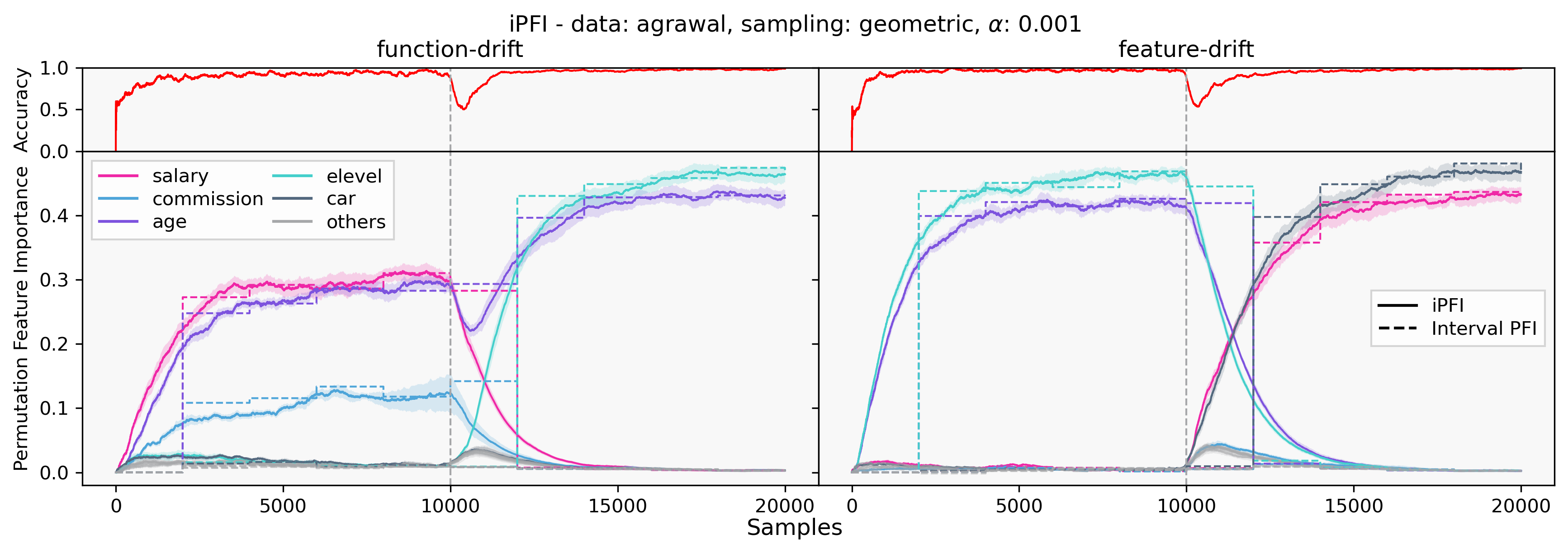
Figure 3: iPFI on two agrawal data streams with induced concept drift. The most important features are colored. The dashed line denotes the batch calculation at set intervals. The dashed vertical line denotes the concept drift.

Figure 4: iPFI with uniform (left) and geometric sampling (right) on elec2 with a feature-drift.

Experiment A: Approximation of Batch PFI

First, we consider the static model setting where models are pre-trained before they are explained on the whole dataset (no incremental learning). This experiment demonstrates that iPFI correctly approximates batch PFI estimation.
We compare iPFI with the classical batch PFI $\hat{\phi}^{(S_{j})}_{\text{batch}}$ for feature $j\in D$, which is computed using the whole static dataset over ten random permutations. We normalize $\hat{\phi}_{\text{iPFI}}^{(S_{j})}$ and $\hat{\phi}_{\text{batch}}^{(S_{j})}$ between 0 and 1, and compute the sum over the feature-wise absolute approximation errors;

$$\text{error}:=\sum_{j\in D}{\left|\hat{\phi}_{\text{iPFI}}^{(S_{j})}-\hat{\phi}_{\text{batch}}^{(S_{j})}\right|}.$$

Table 1 shows the median and interquartile range (IQR) (difference between the first and third quartile) of the error based on ten random orderings of each dataset. Figure 2 shows the approximation quality of iPFI with geometric and uniform sampling per feature for the bank dataset. In the static modeling case, there is no clear difference between geometric and uniform sampling. However, in the dynamic modeling context under drift, the sampling strategy has a substantial effect on the iPFI estimates.

Experiment B: Online PFI Calculation under Drift

In this experiment, we consider a dynamic modeling scenario. Here, instead of a pre-trained model, we fit ARF models incrementally on real data streams and compute iPFI on the fly. For the sake of clarity and simplicity, we only present results for ARF models here. However, as our approach is inherently model-agnostic, any incremental model (implemented for example in river) can be explained. As a baseline, we compare our approach to the interval PFI for feature $j\in D$, which computes the PFI over fixed time intervals during the online learning process with ten random permutations in each interval. This can be seen as a naive implementation of iPFI with large gaps of uncertainty and a substantial time delay. With the synthetic agrawal stream we induce two kinds of real concept drifts: First, we switch the classification function of the data generator, which we refer to as function-drift (changing the functional dependency but retaining the distribution of $X$). Second, we switch the values of two or more features with each other, which we refer to as feature-drift (changing the functional dependency by changing the distribution of $X$). Note that feature-drift can also be applied to datasets, where the classification function is unknown. Figure 3 showcases how well iPFI reacts to both concept drift scenarios. Both concept drifts are induced in the middle of the data stream (after 10,000 samples). For the function-drift example (Figure 3, left), the agrawal classification function was switched from Agrawal, Imielinski, and Swami (1993)’s concept $1$ to concept $2$. Theoretically, only two features should be important for both concepts: For the first concept the pink salary and the purple age features are needed, and for the second concept the classification function relies on the cyan education and the purple age features. However, the ARF model also relies on the blue commission feature, which can be explained as commission directly depends on salary. In the feature-drift scenario (Figure 3, right), the ARF model adapts to a sudden drift where both important features (education and age) are switched with two unimportant features (car and salary). In both scenarios iPFI instantly detects the shifts in importance.

From both simulations, it is clear that iPFI and its anytime computation has clear advantages over interval PFI. In fact, iPFI quickly reacts to changes in the data distribution while still closely matching the “ground-truth” results of the batch-interval computation. For further concept drift scenarios, we refer to the supplementary material.

Experiment C: Geometric vs. Uniform Sampling

Lastly, we focus on the question, which sampling strategy to prefer in which learning environments. We conclude that geometric sampling should be applied under feature-drift scenarios, as the choice of sampling strategy substantially impacts iPFI’s performance in concept drift scenarios where feature distributions change. If a dynamic model adapts to changing feature distributions, and the PFI is estimated with samples from the outdated distribution, the resulting replacement samples are outside the current data manifold. Estimating PFI by using this data can result in skewed estimates, as illustrated in Figure 4. There, we induce a feature-drift by switching the values of the most important feature for an ARF model on elec2 with a random feature. The uniform sampling strategy (Figure 4, left) is incapable of matching the “ground-truth” interval PFI estimation like the geometric sampling strategy (Figure 4, right). Hence, in dynamic learning environments like data stream analytics or continual learning, we recommend applying a sampling strategy that focuses on more recent samples, such as geometric distributions. For applications without drift in the feature-space like progressive data science, uniform sampling strategies, which evenly distribute the probability of a data point being sampled across the data stream, may still be preferred.

For further experiments on different parameters, we again refer to the supplement. Therein, we show that the smoothing parameter $\alpha$ substantially effects iPFI’s FI estimates. Like any smoothing mechanism, this parameter controls the deviation of iPFI’s estimates. This parameter should be set individually for the task at hand. In our experiment, values between $\alpha=0.001$ (conservative) and $\alpha=0.01$ (reactive) appeared to be reasonable.

Conclusion and Future Work

In this work, we considered global FI as a statistic measure of change in the model’s risk when features are marginalized. We discussed PFI as an approach to estimate feature importance and proved that only appropriately scaled permutation tests are unbiased estimators. In this case, the expectation over the sampling strategy (expected PFI) then corresponds to the model reliance U-Statistic (Fisher, Rudin, and Dominici 2019).

Based on this notion, we presented iPFI, an efficient model-agnostic algorithm to incrementally estimate FI by averaging over repeated realizations of a sampling strategy. We introduced two incremental sampling strategies and established theoretical results for the expectation over the sampling strategy (expected iPFI) to control the approximation error using iPFI’s parameters. On various benchmark datasets, we demonstrated the efficacy of our algorithms by comparing them with the batch PFI baseline method in a static progressive setting as well as with interval-based PFI in a dynamic incremental learning scenario with different types of concept drift and parameter choices.

Applying XAI methods incrementally to data stream analytics offers unique insights into models that change over time. In this work, we rely on PFI as an established and inexpensive FI measure. Other computationally more expensive approaches (such as SHAP) address some limitations of PFI. As our theoretical results can be applied to arbitrary feature subsets, analyzing these methods in the dynamic environment offers interesting research opportunities. In contrast to this work’s technical focus, analyzing the dynamic XAI scenario through a human-focused lens with human-grounded experiments is paramount (Doshi-Velez and Kim 2017).

Appendix A Proofs

In the following, we provide the proofs of all theorems. We further present more general results that are stated as propositions.

Theorem 6.

The expected PFI (model reliance) can be rewritten as a normalized expectation over uniformly random permutations, i.e.

$$\bar{\phi}^{(S_{j})}=\frac{N}{N-1}\mathbb{E}_{\varphi\sim\text{unif}(\mathfrak{S}_{N})}\left[\hat{\phi}^{(S_{j})}_{\varphi}\right].$$ (8)

Proof.

We write $f(z_{n},z_{m}):=\|h(x_{n}^{(\bar{S_{j}})},x_{m}^{(S_{j})})-y_{n}\|-\|h(x_{n})-y_{n}\|$ and compute the expectation over randomly sampled permutations $\varphi\in\mathfrak{S}_{N}$. Each permutation has probability $\frac{1}{N!}$, which yields

$$\mathbb{E}_{\varphi}[\hat{\phi}^{(S_{j})}_{\varphi}] =\frac{1}{N!}\sum_{\varphi\in\mathfrak{S}_{N}}\hat{\phi}^{(S_{j})}_{\varphi}$$

$$=\frac{1}{N}\frac{1}{N!}\sum_{n=1}^{N}\sum_{\varphi\in\mathfrak{S}_{N}}f(z_{n},z_{\varphi(n)})$$

$$=\frac{1}{N}\frac{1}{N!}\sum_{n=1}^{N}\sum_{m=1}^{N}(N-1)!f(z_{n},z_{m})$$

$$=\frac{1}{N}\frac{1}{N}\sum_{n=1}^{N}\sum_{m\neq n}f(z_{n},z_{m})$$

$$=\frac{1}{N}\frac{1}{N}\sum_{n=1}^{N}\sum_{m\neq n}\|h(x_{n},x_{m})-y_{n}\|$$

$$-\frac{N-1}{N^{2}}\sum_{n=1}^{N}\|h(x_{n})-y_{n}\|,$$

where we used in the third line that there are $(N-1)!$ permutations with $\varphi(n)=m$. We thus conclude,

$$\frac{N}{N-1}\mathbb{E}_{\varphi}[\hat{\phi}^{(S_{j})}_{\varphi}] =\hat{e}_{\text{switch}}-\hat{e}_{\text{orig}}=\bar{\phi}^{(S_{j})}.$$

∎

Theorem 7 (Bias for static Model).

If $h\equiv h_{t}$, then

$$\phi^{(S_{j})}(h)-\bar{\phi}^{(S_{j})}_{t}=(1-\alpha)^{t-t_{0}+1}\phi^{(S_{j})}(h).$$

Proof.

We consider the more general estimator $\tilde{\phi}^{(S)}_{t}:=\mathbb{E}_{\varphi}[\sum_{s=t_{0}}^{t}w_{s}\hat{\lambda}^{(S)}_{t}(x_{t},x_{\varphi_{t}},y_{t})]$ and prove a more general result that can be used for arbitrary sampling and aggregation techniques.

Proposition 1.

If $h\equiv h_{t}$, then

$$\phi^{(S)}(h)-\mathbb{E}[\tilde{\phi}^{(S)}_{t}]=(1-\mu_{w})\phi^{(S)}(h)$$

with $\mu_{w}:=\sum_{s=t_{0}}^{t}w_{s}$.

Proof.

As each $\hat{\lambda}_{s}^{(S)}$ is an unbiased estimator of $\phi^{(S)}(h_{s})$, we have $\mathbb{E}[\tilde{\phi}^{(S)}_{t}]=\sum_{s=t_{0}}^{t}w_{s}\phi^{(S)}(h)=\mu_{w}\phi^{(S)}(h)$, where we used $(\varphi)_{t_{0}\leq s\leq t}\perp(X,Y)$. ∎

The result then follows directly, as $\bar{\phi}^{(S)}=\tilde{\phi}^{(S)}$ for $w_{s}:=\alpha(1-\alpha)^{t-s}$, $\mu_{w}=1-(1-\alpha)^{t-t_{0}+1}$ and $S:=S_{j}$.

∎

Theorem 8 (Variance for static Model).

If $h_{t}\equiv h$ and $\mathbb{V}[\|h(X_{s}^{(\bar{S_{j}})},X_{r}^{(S_{j})})-Y_{s}\|-\|h(X_{s})-Y_{s}\|]<\infty$, then

Uniform: $$\mathbb{V}\left[\lim_{t\to\infty}\bar{\phi}_{t}^{(S_{j})}\right]=\mathcal{O}(-\alpha\log(\alpha)).$$

Geometric: $$\mathbb{V}\left[\lim_{t\to\infty}\bar{\phi}_{t}^{(S_{j})}\right]=\mathcal{O}(\alpha)+\mathcal{O}(p).$$

Proof.

We again consider the more general estimator $\tilde{\phi}^{(S)}_{t}:=\mathbb{E}_{\varphi}[\sum_{s=t_{0}}^{t}w_{s}\hat{\lambda}^{(S)}_{t}(x_{t},x_{\varphi_{t}},y_{t})]$ and prove a result, that can be used for arbitrary sampling and aggregation techniques.

Proposition 2.

For $\varphi$ from (5) with $\varphi_{s}\perp\varphi_{r}$ for $r<s$ and $p_{s,r}\leq p_{s^{\prime},r}$ for $s>s^{\prime}$, i.e., the probability to sample a previous observation $r$ is non-increasing over time, it holds

$$\mathbb{V}\left[\tilde{\phi}_{t}^{(S)}\right]\leq 4\sigma_{w}^{2}\sigma_{2}^{2}+2\sigma_{2}^{2}\sum_{s=t_{0}}^{t}\sum_{s^{\prime}=t_{0}}^{s-1}w_{s}w_{s^{\prime}}\underbrace{\sum_{r=0}^{s^{\prime}-1}p_{s^{\prime},r}^{2}}_{=:\mathcal{I}_{\varphi}(s)},$$

provided that $\sigma_{2}^{2}:=\mathbb{V}[f(Z_{s},Z_{r})]<\infty$ and with $\sigma^{2}_{w}:=\sum_{s=0}^{t}w_{s}^{2}$.

Proof.

We denote $f(Z_{s},Z_{r}):=\|h(X_{s}^{(\bar{S_{j}})},X_{r}^{(S)})-Y_{s}\|-\|h(X_{s})-Y_{s}\|$. Using $p_{s,r}:=\mathbb{P}(\varphi_{s}=r)$ and properties of variance, we can write

$$\mathbb{V}[\tilde{\phi}_{t}]=\mathbb{V}[\sum_{s=t-N+1}^{t}w_{s}\sum_{r=0}^{s-1}p_{r,s}f(Z_{s},Z_{r})]$$

$$=\sum_{s,s^{\prime}=t_{0}}^{t}w_{s}w_{s^{\prime}}\sum_{r=0}^{s-1}\sum_{r^{\prime}=0}^{s^{\prime}-1}p_{s,r}p_{s^{\prime},r^{\prime}}\text{cov}((s,r),(s^{\prime},r^{\prime})),$$

where $\text{cov}((s,r),(s^{\prime},r^{\prime})):=\text{cov}(f(Z_{s},Z_{r}),f(Z_{s^{\prime}},Z_{r^{\prime}}))$ denotes the covariance of the two random variables. The above sum ranges over all possible combinations of pairs $(s,r)$, where $s=t_{0}\dots,t$ and $r=0,\dots,s-1$. As $r<s$ and $r^{\prime}<s^{\prime}$, it holds $|\{s,s^{\prime},r,r^{\prime}\}|\geq 2$. When $|\{s,s^{\prime},r,r^{\prime}\}|=2$ then $s=s^{\prime}$ and $r=r^{\prime}$ and the covariance reduces to the variance. When none of the indices match, i.e., $|\{s,s^{\prime},r,r^{\prime}\}|=4$, then the covariance is zero, due to the independence assumption. When exactly one index matches, then there are three possible cases:

• case 1: $s=s^{\prime},r\neq r^{\prime}$,

• case 2: $s\neq s^{\prime},r\neq r$ with $r^{\prime}=s$ or $s^{\prime}=r$

• case 3: $s\neq s^{\prime},r=r^{\prime}$.

Case 2 yields the same covariances due to the iid assumption and the symmetric of the covariance. For case 1, with $\mathbb{E}_{(Z_{s},Z_{r})}[f(Z_{s},Z_{r})]=\mathbb{E}_{Z_{s}}\mathbb{E}_{Z_{r}}[f(Z_{s},Z_{r})]=\phi^{(S)}(h)$, we denote $\tilde{f}(Z_{s},Z_{r}):=f(Z_{s},Z_{r})-\phi^{(S)}(h)$ to compute the covariance as

$$\text{cov}((s,r),(s^{\prime},r^{\prime})) =\mathbb{E}[\tilde{f}(Z_{s},Z_{r})\tilde{f}(Z_{s},Z_{r^{\prime}})]$$

$$=\mathbb{E}_{Z_{s}}[\mathbb{E}_{Z_{r}}[\tilde{f}(Z_{s},Z_{r})]\mathbb{E}_{Z_{r^{\prime}}}[\tilde{f}(Z_{s},Z_{r^{\prime}})]]$$

$$=\mathbb{E}_{Z_{s}}[\mathbb{E}_{Z_{r}}[\tilde{f}(Z_{s},Z_{r})]^{2}]$$

$$=\mathbb{V}_{Z_{s}}[\mathbb{E}_{Z_{r}}[f(Z_{s},Z_{r})]],$$

where we have used $\mathbb{E}_{Z_{s}}[\mathbb{E}_{Z_{r}}[\tilde{f}(Z_{s},Z_{r})]]=\phi^{(S)}(h)$ as well as the iid assumption multiple times, in particular when $\mathbb{E}_{Z_{r}}[f(Z_{s},Z_{r})]=\mathbb{E}_{Z_{r^{\prime}}}[f(Z_{s},Z_{r^{\prime}})]$. The same arguments apply for the second argument for case 3, as

$$\text{cov}((s,r),(s^{\prime},r^{\prime}))=\mathbb{V}_{Z_{r}}[\mathbb{E}_{Z_{s}}[f(Z_{s},Z_{r})]].$$

We thus summarize

$$\text{cov}((s,r),(s^{\prime},r^{\prime}))=\begin{cases}\mathbb{V}[f(Z_{s},Z_{r})],\text{ if }s=s^{\prime},r=r^{\prime}\\ \mathbb{V}_{Z_{s}}[\mathbb{E}_{Z_{r}}[f(Z_{s},Z_{r})]],\text{ if case 1}\\ \text{cov}((s,r),(s^{\prime},r^{\prime})),\text{ if case 2}\\ \mathbb{V}_{Z_{r}}[\mathbb{E}_{Z_{s}}[f(Z_{s},Z_{r})]],\text{ if case 3}\\ 0,\text{ if }|\{s,s^{\prime},r,r^{\prime}\}|=4.\end{cases}$$

By the Cauchy-Schwarz inequality all covariances are bounded by $\sigma_{2}^{2}:=\mathbb{V}[f(Z_{s},Z_{r})]$. With $I:=\{t_{0},\dots,t\}$ and $I_{s}:=\{0,\dots,s-1\}$ and $Q_{2}:=\{(s,r):s=s^{\prime}\in I,r=r^{\prime}\in I_{s}\}$ $Q_{3}:=\{(s,s^{\prime},r,r^{\prime}):s,s^{\prime}\in I,r\in I_{s},r^{\prime}\in I_{r^{\prime}},|\{s,s^{\prime},r,r^{\prime}\}|=3\}$. We thus obtain

$$\mathbb{V}[\tilde{\phi}_{t}^{(S)}] =\sigma_{2}^{2}\sum_{(s,r)\in Q_{2}}w_{s}^{2}p_{s,r}^{2}$$

$$+\sum_{(s,s^{\prime},r,r^{\prime})\in Q_{3}}w_{s}w_{s^{\prime}}p_{s,r}p_{s^{\prime},r^{\prime}}\text{cov}((s,r),(s^{\prime},r^{\prime})).$$

For the first sum, we have

$$\sum_{(s,r)\in Q_{2}}w_{s}^{2}p_{s,r}^{2}\leq\sum_{(s,r)\in Q_{2}}w_{s}^{2}p_{s,r}=\sum_{s=t_{0}}^{t}w_{s}^{2}=\sigma_{w}^{2}.$$

For the second sum, $Q_{3}$ decomposes into the three cases. For case 1,

$$\sum_{\begin{subarray}{c}(s,s^{\prime},r,r^{\prime})\in Q_{3}\\ s=s^{\prime},r\neq r^{\prime}\end{subarray}}w_{s}w_{s^{\prime}}p_{s,r}p_{s,r^{\prime}} =\sum_{s=t_{0}}^{t}w_{s}w_{s^{\prime}}\sum_{\begin{subarray}{c}(r,r^{\prime})\in I_{s}^{2}\\ r\neq r^{\prime}\end{subarray}}p_{s,r}p_{s,r^{\prime}}$$

$$\leq\sum_{s=t_{0}}^{t}w_{s}^{2}(\sum_{r=0}^{s-1}p_{s,r})^{2}=\sigma_{w}^{2}.$$

For case 2 w.l.o.g assume $r=s^{\prime}$, which implies $s>s^{\prime}$ and thus $w_{s}\geq w_{s^{\prime}}$, then

$$\sum_{\begin{subarray}{c}(s,s^{\prime},r,r^{\prime})\in Q_{3}\\ s\neq s^{\prime},r\neq r^{\prime},s^{\prime}=r\end{subarray}}w_{s}w_{s^{\prime}}p_{s,s^{\prime}}p_{s^{\prime},r^{\prime}} =\sum_{s=t_{0}}^{t}w_{s}\sum_{s^{\prime}=t_{0}}^{s-1}w_{s^{\prime}}p_{s,s^{\prime}}$$

$$\leq\sum_{s=t_{0}}^{t}w_{s}^{2}=\sigma_{w}^{2}.$$

For case 3, we have

$$\sum_{\begin{subarray}{c}(s,s^{\prime},r,r^{\prime})\in Q_{3}\\ s\neq s^{\prime},r=r^{\prime}\end{subarray}}w_{s}w_{s^{\prime}}p_{s,r}p_{s^{\prime},r} =\sum_{\begin{subarray}{c}(s,s^{\prime})\in I^{2}\\ s\neq s^{\prime}\end{subarray}}w_{s}w_{s^{\prime}}\sum_{r=0}^{\min(s,s^{\prime})-1}p_{s,r}p_{s^{\prime},r}$$

$$=2\sum_{\begin{subarray}{c}(s,s^{\prime})\in I^{2}\\ s>s^{\prime}\end{subarray}}w_{s}w_{s^{\prime}}\sum_{r=0}^{s^{\prime}-1}p_{s,r}p_{s^{\prime},r}$$

$$\leq 2\sum_{\begin{subarray}{c}(s,s^{\prime})\in I^{2}\\ s>s^{\prime}\end{subarray}}w_{s}w_{s^{\prime}}\sum_{r=0}^{s^{\prime}-1}p_{s^{\prime},r}^{2}.$$

In summary, we conclude

$$\mathbb{V}\left[\tilde{\phi}_{t}^{(S)}\right]\leq 4\sigma_{w}^{2}\sigma_{2}^{2}+2\sigma_{2}^{2}\sum_{s=t_{0}}^{t}\sum_{s^{\prime}=t_{0}}^{s-1}w_{s}w_{s^{\prime}}\sum_{r=0}^{s^{\prime}-1}p_{s^{\prime},r}^{2}.$$

∎

The last sum depends on both the choices of weights $w_{s}$ and the collision probability $\mathcal{I}_{\varphi}(s)=\sum_{r=0}^{s-1}p_{s,r}^{2}=P(Q_{1}=Q_{2})$ for $Q_{1},Q_{2}\overset{iid}{\sim}\mathbb{P}_{\varphi_{s}}$, which is related to the Rényi entropy (Rényi 1961). The variance increases with the collision probabilities of the sampling strategy, in particular $\mathcal{I}_{\text{unif}}(s)=\frac{1}{s}$ and $\mathcal{I}_{\text{geom}}(s)=\frac{p}{2-p}(1+(1-p)^{2(s-t_{0})+1})$ for uniform and geometric sampling, respectively.

Lemma 1.

For geometric sampling and $p\in(0,1)$ it holds

$$\mathcal{I}_{\text{geom}}(s)=\sum_{r=0}^{s-1}p^{2}_{s,r}=\frac{p}{2-p}(1+(1-p)^{2(s-t_{0})+1}).$$

Proof.

The probabilities for geometric sampling are

$$p_{s,r}=\begin{cases}p\cdot(1-p)^{s-r-1},r>t_{0}=\frac{1}{p}\\ p\cdot(1-p)^{s-t_{0}},r\leq t_{0}=\frac{1}{p}.\end{cases}$$

Then

$$\mathcal{I}_{\text{geom}}(s) =\sum_{r=0}^{s-1}p^{2}_{s,r}$$

$$=\sum_{r=0}^{t_{0}-1}p^{2}\cdot(1-p_{r})^{2(s-t_{0})}+\sum_{r=t_{0}}^{s-1}p^{2}(1-p)^{2(s-r-1)}$$

$$=t_{0}\cdot p^{2}\cdot(1-p)^{2(s-t_{0})}+\sum_{r=t_{0}}^{s-1}p^{2}(1-p)^{2(s-r-1)}$$

$$=p\cdot(1-p)^{2(s-t_{0})}+p^{2}\sum_{r=0}^{s-t_{0}-1}(1-p)^{2r}$$

$$=p\cdot(1-p)^{2(s-t_{0})}+p^{2}\frac{1-(1-p)^{2(s-t_{0})}}{1-(1-p)^{2}}$$

$$=p\cdot(1-p)^{2(s-t_{0})}+\frac{p}{2-p}(1-(1-p)^{2(s-t_{0})})$$

$$=\frac{p}{2-p}(1+(1-p)^{2(s-t_{0})+1}).$$

∎

We now apply Proposition 2 to our particular estimator $\bar{\phi}^{(S)}=\tilde{\phi}^{(S)}$ with $w_{s}:=\alpha(1-\alpha)^{t-s}$ and take the limit for $t\to\infty$. Note that both uniform and geometric sampling fulfill the condition of the theorem. Furthermore, we have $\sigma^{2}_{w}=\alpha^{2}\sum_{s=0}^{t-t_{0}}(1-\alpha)^{s}\nearrow\frac{\alpha}{2-\alpha}$.

Uniform Sampling

For uniform sampling, we have

$$\mathbb{V}[\bar{\phi}_{t}^{(S)}] \leq\frac{\alpha}{2-\alpha}4\sigma_{2}^{2}+2\sigma_{2}^{2}\sum_{s=t_{0}}^{t}\sum_{s^{\prime}=t_{0}}^{s-1}\alpha^{2}\frac{(1-\alpha)^{t-s+t-s^{\prime}}}{s^{\prime}}$$

$$\leq\frac{\alpha}{2-\alpha}4\sigma_{2}^{2}+2\sigma_{2}^{2}\alpha^{2}\sum_{s=0}^{t-t_{0}}(1-\alpha)^{s}\sum_{s^{\prime}=0}^{t-t_{0}}\frac{(1-\alpha)^{s^{\prime}}}{t-s^{\prime}}$$

For the first sum, we have $\alpha\sum_{s=0}^{t-t_{0}}(1-\alpha)^{s}\nearrow 1$ for $t\to\infty$. For the second sum

$$\alpha\sum_{s^{\prime}=0}^{t-t_{0}}\frac{(1-\alpha)^{s^{\prime}}}{t-s^{\prime}} \leq\alpha(\sum_{\begin{subarray}{c}s^{\prime}=0\\ s^{\prime}\geq t/2\end{subarray}}^{t-t_{0}}(1-\alpha)^{s^{\prime}}+1+\sum_{\begin{subarray}{c}s^{\prime}=1\\ s^{\prime}<t/2\end{subarray}}^{t-t_{0}}\frac{(1-\alpha)^{s^{\prime}}}{s^{\prime}})$$

$$\leq(1-\alpha)^{t/2}-(1-\alpha)^{t-t_{0}+1}+\alpha-\alpha\log(\alpha)$$

$$\overset{t\to\infty}{\longrightarrow}\alpha-\alpha\log(\alpha).$$

Hence,

$$\mathbb{V}[\lim_{t\to\infty}\bar{\phi}_{t}^{(S)}]=\mathcal{O}(-\alpha\log(\alpha)).$$

Geometric Sampling

For geometric sampling, we have

$$\mathbb{V}[\bar{\phi}_{t}^{(S)}] \leq\underbrace{\frac{\alpha}{2-\alpha}4\sigma_{2}^{2}}_{=\mathcal{O}(\alpha)}$$

$$+2\sigma_{2}^{2}\underbrace{\alpha^{2}\sum_{s=t_{0}}^{t}\sum_{s^{\prime}=t_{0}}^{s-1}(1-\alpha)^{t-s+t-s^{\prime}}]}_{=:q(\alpha)}\mathcal{I}_{\text{geom}}(s).$$

For the second term it is enough to show that $0<\lim_{t\to\infty}q(\alpha)<\infty$ to prove the result, as $\mathcal{I}_{\text{geom}}(s)=\mathcal{O}(p)$. By using the properties of geometric progression, we obtain

$$q(\alpha) =\alpha\sum_{s=t_{0}}^{t}(1-\alpha)^{t-s}\alpha\sum_{s^{\prime}=t-s}^{t-t_{0}}(1-\alpha)^{s^{\prime}}$$

$$=\alpha\sum_{s=t_{0}}^{t}(1-\alpha)^{t-s}((1-\alpha)^{t-s}-(1-\alpha)^{t-t_{0}+1})$$

$$=\alpha\sum_{s=0}^{t-t_{0}}(1-\alpha)^{s}((1-\alpha)^{s}-(1-\alpha)^{t-t_{0}+1})$$

$$=\underbrace{\alpha\sum_{s=0}^{t-t_{0}}(1-\alpha)^{2s}}_{\nearrow\frac{1}{2-\alpha}}-(1-\alpha)^{t-t_{0}+1}\underbrace{\alpha\sum_{s=0}^{t-t_{0}}(1-\alpha)^{s}}_{\nearrow 1}$$

$$\overset{t\to\infty}{\longrightarrow}\frac{1}{2-\alpha}.$$

Hence,

$$\mathbb{V}[\lim_{t\to\infty}\bar{\phi}_{t}^{(S)}]\leq\mathcal{O}(\alpha)+2\sigma_{2}^{2}\frac{2}{2-\alpha}\frac{p}{2-p}=\mathcal{O}(\alpha)+\mathcal{O}(p).$$

∎

Theorem 9 (Bias for changing Model).

If $\Delta(h_{s},h_{t})\leq\delta$ and $\Delta_{S}(h_{s},h_{t})\leq\delta_{S}$ for $t_{0}\leq s\leq t$, then

$$|\bar{\phi}^{(S_{j})}_{t}-\phi^{(S_{j})}(h_{t})|\leq\delta_{S}+\delta+\mathcal{O}((1-\alpha)^{t}).$$

Proof.

We again consider the more general estimator $\tilde{\phi}^{(S)}_{t}:=\mathbb{E}_{\varphi}[\sum_{s=t_{0}}^{t}w_{s}\hat{\lambda}^{(S)}_{t}(x_{t},x_{\varphi_{t}},y_{t})]$ and prove a more general result.

Proposition 3.

If $\Delta(h_{s},h_{t})\leq\delta$ and $\Delta_{S}(h_{s},h_{t})\leq\delta_{S}$ for $t_{0}\leq s\leq t$, then $|\mathbb{E}[\hat{\phi}^{(S)}_{t}]-\phi^{(S)}(h_{t})|\leq\mu_{w}(\delta_{S}+\delta)+|(1-\mu_{w})\phi^{(S)}(h_{t})|$.

Proof.

For the proof, we first show that for two models $h_{s},h_{t}$ and a subset $S\subset D$, it holds that $|\phi^{(S)}(h_{t})-\phi^{(S)}(h_{s})|\leq\Delta_{S}(h_{s},h_{t})+\Delta(h_{s},h_{t})$. This follows directly from the reverse triangle inequality for $f_{S}^{\Delta}(x^{(\bar{S})},h_{s},h_{t})\geq\mathbb{E}_{\tilde{X}}[\|h_{t}(x^{(\bar{S})},\tilde{X})-y\|-\|y-h_{s}(x^{(\bar{S})},\tilde{X})\|]$. The result then follows directly by definition, the observation that $\hat{\lambda}_{s}^{(S)}$ is an unbiased estimate of $\phi^{(S)}(h_{s})$, as

$$|\mathbb{E}[\bar{\phi}^{(S)}_{t}]-\phi^{(S)}(h_{t})| =|(\sum_{s=t_{0}}^{t}w_{s}\phi^{(S)}(h_{s}))-\phi^{(S)}(h_{t})|$$

$$\leq\sum_{s=t_{0}}^{t}w_{s}\underbrace{|\phi^{(S)}(h_{s})-\phi^{(S)}(h_{t})|}_{\leq\delta+\delta_{S}}$$

$$+|(\sum_{s=t_{0}}^{t}w_{s}-1)\phi^{(S)}(h_{t})|$$

$$\leq\mu_{w}(\delta+\delta_{S})+\underbrace{|(1-\mu_{w})\phi^{(S)}(h_{t})|}_{\text{bias for static model}}.$$

∎

With $\mu_{w}=1-(1-\alpha)^{t-t_{0}+1}$ our special case follows immediately. ∎

Theorem 10 (Variance for changing Model).

If

$$\text{cov}(f_{s}(Z_{s},Z_{r}),f_{s^{\prime}}(Z_{s^{\prime}},Z_{r^{\prime}}))\leq\sigma_{\text{max}}^{2}$$ (9)

for $t_{0}\leq s,s^{\prime}\leq t$, $r<s$ and $r^{\prime}<s^{\prime}$, then for a sequence of models $(h_{t})_{t\geq 0}$ the results of Theorem 8 apply.

Proof.

In all proofs a changing model $h_{t}$ adds a time dependency on the function $f_{s}(Z_{s},Z_{r}):=\|h_{s}(X_{s}^{(\bar{S})},X_{r}^{(S)})-Y_{s}\|-\|h_{s}(X_{s})-Y_{s}\|$. Instead of bounding the covariances by $\sigma_{2}^{2}$, we now bound the covariances of the time-dependent functions by $\sigma_{\text{max}}^{2}$. This only directly affects Proposition 2, as

$$\mathbb{V}[\bar{\phi}_{t}^{(S)}] =\mathbb{V}[\sum_{s=t-N+1}^{t}w_{s}\sum_{r=0}^{s-1}p_{r,s}f_{s}(Z_{s},Z_{r})]$$

$$=\sum_{s,s^{\prime}=t_{0}}^{t}w_{s}w_{s^{\prime}}\sum_{r=0}^{s-1}\sum_{r^{\prime}=0}^{s^{\prime}-1}p_{s,r}p_{s^{\prime},r^{\prime}}\text{cov}((s,r),(s^{\prime},r^{\prime}))$$

$$\leq\sigma^{2}_{\text{max}}\sum_{s,s^{\prime}=t_{0}}^{t}w_{s}w_{s^{\prime}}\sum_{r=0}^{s-1}\sum_{r^{\prime}=0}^{s^{\prime}-1}p_{s,r}p_{s^{\prime},r^{\prime}}.$$

All remaining arguments and proofs are still valid for a changing model due to the iid assumption. ∎

Appendix B Link to FI used in SAGE

Our definition of FI aligns with the definition of FI $v_{h}(S)$ given by Covert, Lundberg, and Lee (2020), which measures the increase in risk when including features in $S$ compared with marginalizing all features. The conditional distribution $X^{(S)}|X^{(\bar{S})}$ coincides with the marginal distribution if $X^{(\bar{S})}\perp X^{(S)}$, which is often assumed in practice (Covert, Lundberg, and Lee 2021, 2020; Lundberg and Lee 2017). It was even suggested that the marginal distribution is conceptually the right choice (Janzing, Minorics, and Bloebaum 2020).

Appendix C Approximation Error for expected PFI

With $f(Z_{n},Z_{m}):=\|h(X_{n}^{(\bar{S_{j}})},X_{m}^{(S_{j})})-Y_{n}\|-\|h(X_{n})-Y_{n}\|$ and symmetric U-statistic kernel $f_{0}(Z_{n},Z_{m}):=\frac{f(Z_{n},Z_{m})+f(Z_{m},Z_{n})}{2}$, we can write

$$\bar{\phi}^{(S_{j})}=\binom{N}{2}^{-1}\sum_{1\leq n<m\leq N}f_{0}(Z_{n},Z_{m}),$$

which is the basic form of a U-statistic and therefore the variance can be computed as

$$\mathbb{V}\left[\bar{\phi}^{(S_{j})}\right]=\binom{N}{2}^{-1}\sum_{c=1}^{2}\binom{2}{c}\binom{N-2}{2-c}\sigma^{2}_{c}=\mathcal{O}(1/N),$$

where $\sigma_{1}^{2}:=\mathbb{V}_{Z_{n}}[\mathbb{E}_{Z_{m}}[f_{0}(Z_{n},Z_{m})]]$ and $\sigma_{2}^{2}:=\mathbb{V}[f_{0}(Z_{n},Z_{m})]$ are assumed to be finite (Hoeffding 1948). For $\epsilon>0$, we then obtain by Chebyshev’s inequality $\mathbb{P}(|\bar{\phi}^{(S_{j})}-\phi^{(S_{j})}(h)|>\epsilon)=\mathcal{O}(1/N)$, as $\bar{\phi}^{(S_{j})}$ is unbiased.

Appendix D Ground-truth PFI for the agrawal stream.

River (Montiel et al. 2020) implements the agrawal (Agrawal, Imielinski, and Swami 1993) data stream with multiple classification functions. In our experiments we consider the following classification function (among others):

Class A: $$((\text{age}<40)\land(50K\leq\text{salary}\leq 100K))\ \lor$$

$$((40\leq\text{age}<60)\land(75K\leq\text{salary}\leq 125K))\ \lor$$

$$((\text{age}\geq 60)\land(25K\leq\text{salary}\leq 75K))$$

Both feature age and salary are uniformly distributed with $X^{(\text{age})}\sim\mathcal{U}_{[20,80]}$ and $X^{(\text{salary})}\sim\mathcal{U}_{[20,150]}$. Given iid. samples from the data stream the classification problem can be transformed into a two-dimensional problem following the above defined classification function. The two-dimensional classification problem is illustrated in Figure. 5. A sample is classified as concept $A$ when it occurs contained in $A_{1}$, $A_{2}$, or $A_{3}$. Otherwise the sample is classified as concept $B$.

The theoretical PFIs can be calculated with the base probability of an sample belonging to concept A ($P(A_{1})=P(A_{2})=P(A_{3})=\frac{5}{39}$) times the probability of switching the class through changing a feature ($P(A_{i}\rightarrow B_{n,m})$) plus the vice versa for a sample originally belonging to concept $B$.

$$\phi^{(\text{age})} =P(A_{1})\cdot P(A_{1}\rightarrow B_{11})+P(B_{11})\cdot P(B_{11}\rightarrow A_{1})$$

$$+P(A_{2})\cdot P(A_{2}\rightarrow B_{21})+P(B_{21})\cdot P(B_{21}\rightarrow A_{2})$$

$$+P(A_{3})\cdot P(A_{3}\rightarrow B_{31})+P(B_{31})\cdot P(B_{31}\rightarrow A_{3})=$$

$$=\frac{5}{39}\cdot\frac{1}{3}+(\frac{5}{13}\cdot\frac{1}{3})\cdot\frac{1}{3}$$

$$+2\cdot(\frac{5}{39}\cdot\frac{1}{2}+(\frac{5}{13}\cdot\frac{1}{3}+\frac{5}{13}\cdot\frac{1}{3}\cdot\frac{1}{2})\cdot\frac{1}{3})\approx$$

$$\approx 0.3419$$

$$\phi^{(\text{salary})} =P(A_{1})\cdot P(A_{1}\rightarrow B_{12})+P(B_{12})\cdot P(B_{12}\rightarrow A_{1})$$

$$+P(A_{2})\cdot P(A_{2}\rightarrow B_{22})+P(B_{22})\cdot P(B_{22}\rightarrow A_{2})$$

$$+P(A_{3})\cdot P(A_{3}\rightarrow B_{32})+P(B_{32})\cdot P(B_{32}\rightarrow A_{3})=$$

$$=3\cdot(\frac{5}{39}\cdot\frac{8}{13}+(\frac{8}{13}\cdot\frac{1}{3})\cdot\frac{5}{13})\approx$$

$$\approx 0.4734$$

Figure 5: Two-Dimensional Classification Problem of the agrawal Data Stream.

Appendix E Experiments

In the following, we give more comprehensive details about the datasets and models used in our experiments.

Dataset Description

adult (Kohavi 1996)

Binary classification dataset that classifies 48842 individuals based on 14 features into yearly salaries above and below 50k. There are six numerical features and eight nominal features.

bank (Moro, Cortez, and Laureano 2011)

Binary classification dataset that classifies 45211 marketing phone calls based on 17 features to decide whether they decided to subscribe a term deposit. There are seven numerical features and ten nominal features.

bike (Fanaee-T and Gama 2014)

Regression dataset that collects the number of bikes in different bike stations of Toulouse over 187470 time stamps. There are six numerical features and two nominal features.

elec2 (Harries 1999)

Binary classification dataset that classifies, if the electricity price will go up or down. The data was collected for 45312 time stamp from the Australian New South Wales Electricity Market and is based on eight features, six numerical and two nominal.

agrawal (Agrawal, Imielinski, and Swami 1993)

Synthetic data stream generator to create binary classification problems to decide whether an indivdual will be granted a loan based on nine features, six numerical and three nominal. There are ten different decision functions available.

stagger (Schlimmer and Granger 1986)

The stagger concepts makes a simple toy classification data stream. The syntethtical data stream generator consists of three independent categorical features that describe the shape, size, and color of an artificial object. Different classification functions can be derived from these sharp distinctions.

Model Description

All models are implemented with the default parameters from scikit-learn (Pedregosa et al. 2011) and River (Montiel et al. 2020) unless otherwise stated.

ARF

The Adaptive Random Forest Classifier (ARF) uses an ensemble of 50 trees with binary splits, ADWIN drift detection and information gain split criterion. We used the default implementation AdaptiveRandomForestClassifier from River with n_models=50 and binary_split=True.

NN

The Neural Network classifier (NN) was implemented with two hidden layers of size $128\times 64$, ReLu activation function and optimized with stochastic gradient descent (ADAM). We used the default implementation MLPClassifier from scikit-learn.

GBT

The Gradient Boosting Tree (GBT) uses 200 estimators and additively builds a decision tree ensemble using log-loss optimization. We used the GradientBoostingClassifier from scikit-learn with n_estimators=200.

LGBM

The LightGBM (LGBM) constitutes a more lightweight implementation of GBT. We used HistGradientBoostingRegressor for regression tasks and HistGradientBoostingClassifier for classification tasks from scikit-learn with the standard parameters.

Hardware Details

The experiments were mainly run on an computation cluster on hyperthreaded Intel Xeon E5-2697 v3 CPUs clocking at with 2.6Ghz. In total the experiments took around 300 CPU hours (30 CPUs for 10 hours) on the cluster. This mainly stems from the number of parameters and different initializations. Before running the experiments on the cluster, the implementations were validated on a Dell XPS 15 9510 containing an Intel i7-11800H at 2.30GHz. The laptop was running for around 12 hours for this validation.

Summary of experiments

Table 2 contains summary information about the supplementary experiments. Table 3 contains additional information for Experiment B and C in the main contribution.

data	image id	sampling	$\boldsymbol{\alpha}$	whole stream				before drift				after drift
		strategy		$\boldsymbol{Q_{2}}$	IQR	$\boldsymbol{Q_{1}}$	$\boldsymbol{Q_{3}}$	$\boldsymbol{Q_{2}}$	IQR	$\boldsymbol{Q_{1}}$	$\boldsymbol{Q_{3}}$	$\boldsymbol{Q_{2}}$	IQR	$\boldsymbol{Q_{1}}$	$\boldsymbol{Q_{3}}$
agrawal	fu. 1	uniform	0.001	0.050	0.054	0.025	0.079	0.075	0.018	0.063	0.080	0.024	0.028	0.009	0.038
		geometric	0.001	0.052	0.060	0.024	0.084	0.071	0.020	0.068	0.088	0.022	0.023	0.014	0.037
		uniform	0.01	0.047	0.075	0.021	0.096	0.098	0.020	0.091	0.111	0.018	0.011	0.017	0.029
		geometric	0.01	0.040	0.080	0.027	0.107	0.116	0.044	0.078	0.122	0.027	0.008	0.021	0.029
	fu. 2	uniform	0.001	0.067	0.060	0.050	0.110	0.064	0.023	0.047	0.070	0.072	0.065	0.058	0.123
		geometric	0.001	0.063	0.066	0.044	0.110	0.059	0.026	0.041	0.067	0.074	0.071	0.051	0.122
		uniform	0.01	0.111	0.135	0.061	0.196	0.208	0.088	0.153	0.240	0.058	0.016	0.052	0.069
		geometric	0.01	0.103	0.088	0.071	0.159	0.166	0.101	0.140	0.241	0.070	0.028	0.059	0.087
	fu. 2, early	uniform	0.001	0.067	0.123	0.035	0.158	0.110	0.060	0.080	0.140	0.064	0.105	0.032	0.137
		geometric	0.001	0.066	0.132	0.036	0.168	0.116	0.067	0.082	0.149	0.063	0.106	0.032	0.138
		uniform	0.01	0.069	0.113	0.052	0.165	0.217	0.043	0.195	0.238	0.066	0.042	0.046	0.088
		geometric	0.01	0.078	0.103	0.055	0.157	0.187	0.020	0.177	0.196	0.069	0.042	0.050	0.092
	fu. 2, late	uniform	0.001	0.071	0.106	0.045	0.151	0.051	0.031	0.042	0.072	0.244	0.231	0.163	0.394
		geometric	0.001	0.081	0.105	0.051	0.156	0.061	0.042	0.041	0.082	0.246	0.230	0.170	0.400
		uniform	0.01	0.117	0.093	0.066	0.159	0.139	0.087	0.069	0.156	0.095	0.091	0.071	0.162
		geometric	0.01	0.103	0.115	0.063	0.178	0.128	0.106	0.065	0.170	0.077	0.101	0.063	0.163
	fu. 3	uniform	0.001	0.079	0.071	0.037	0.108	0.097	0.026	0.086	0.111	0.032	0.037	0.016	0.053
		geometric	0.001	0.081	0.078	0.035	0.113	0.095	0.036	0.084	0.119	0.029	0.036	0.017	0.053
		uniform	0.01	0.097	0.108	0.053	0.161	0.149	0.044	0.134	0.178	0.056	0.009	0.051	0.060
		geometric	0.01	0.124	0.067	0.087	0.153	0.142	0.022	0.135	0.157	0.090	0.038	0.074	0.112
	fe. 1	uniform	0.001	0.048	0.102	0.018	0.121	0.021	0.036	0.017	0.054	0.087	0.177	0.043	0.220
		geometric	0.001	0.035	0.091	0.015	0.106	0.023	0.031	0.018	0.049	0.047	0.117	0.008	0.125
		uniform	0.01	0.062	0.044	0.034	0.077	0.072	0.023	0.056	0.079	0.046	0.037	0.030	0.067
		geometric	0.01	0.044	0.052	0.035	0.087	0.079	0.047	0.042	0.089	0.043	0.014	0.032	0.046
stagger	fu. 1	uniform	0.001	0.018	0.118	0.014	0.132	0.009	0.005	0.007	0.012	0.132	0.443	0.075	0.518
		geometric	0.001	0.018	0.117	0.015	0.131	0.008	0.006	0.005	0.011	0.131	0.440	0.075	0.515
elec2	fe. 1	uniform	0.001	0.270	0.305	0.042	0.347	0.041	0.061	0.033	0.093	0.353	0.068	0.311	0.378
		geometric	0.001	0.037	0.039	0.033	0.072	0.037	0.066	0.032	0.098	0.037	0.022	0.036	0.057
	fe. 1, gradual	uniform	0.001	0.158	0.263	0.050	0.313	0.048	0.075	0.025	0.101	0.321	0.089	0.283	0.372
		geometric	0.001	0.037	0.024	0.027	0.051	0.040	0.069	0.026	0.095	0.037	0.013	0.028	0.041

Table 2: Summary of additional concept drift experiments on agrawal, stagger, and elec2. The image identifier point to the subsequent section of figures. $Q_{2}$ denotes the median of the error described in Experiment A computed for iPFI and interval PFI (solid line vs. dashed line in the Figures). The interquartile range is calculated between $Q_{1}$ and $Q_{3}$.

data	exp.	image	whole stream				before drift				after drift
		facet	$\boldsymbol{Q_{2}}$	IQR	$\boldsymbol{Q_{1}}$	$\boldsymbol{Q_{3}}$	$\boldsymbol{Q_{2}}$	IQR	$\boldsymbol{Q_{1}}$	$\boldsymbol{Q_{3}}$	$\boldsymbol{Q_{2}}$	IQR	$\boldsymbol{Q_{1}}$	$\boldsymbol{Q_{3}}$
agrawal	B	function- drift	0.052	0.060	0.024	0.084	0.071	0.020	0.068	0.088	0.022	0.023	0.014	0.037
		feature- drift	0.035	0.091	0.015	0.106	0.023	0.031	0.018	0.049	0.047	0.117	0.008	0.125
elec2	C	uniform sampling	0.270	0.305	0.042	0.347	0.041	0.061	0.033	0.093	0.353	0.068	0.311	0.378
		geometric sampling	0.037	0.039	0.033	0.072	0.037	0.066	0.032	0.098	0.037	0.022	0.036	0.057

Table 3: Summary of experiment B and C’s iPFI’s error against interval PFI (solid line vs. dashed line in the Figures).

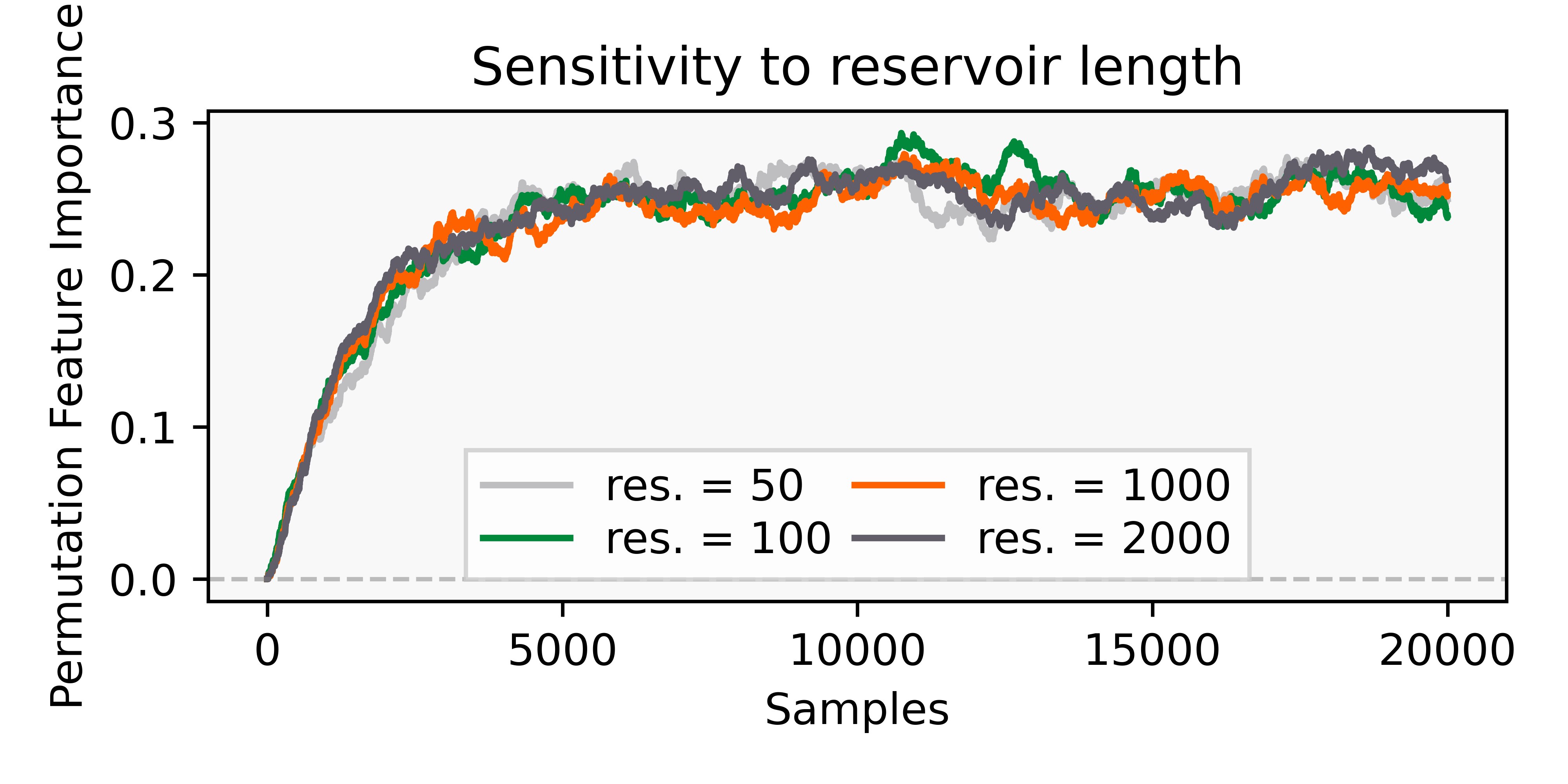
Figure 6: The importance of the nswprice feature for an ARF model training on elec2 for different values of $\alpha$ (left) and reservoir length (right) iPFI parameters.

Parameter Analysis

In addition to the analysis of the sampling strategy, we further analyzed the effect of $\alpha$ smoothing parameter and the length of the reservoir used for sampling. Figure 6 shows how the $\alpha$ smoothing parameter has a substantial effect on the iPFI estimates. The length of the reservoir has no large effect on the estimates. For both sensitivity analysis experiments, iPFI with geometric sampling is applied on an ARF and elec2. only the important nswprice feature is plotted. For each parameter value a single run is presented.

Figure 7: iPFI on agrawal with a function-drift (fu. 1) after 10k samples with $\alpha=0.001$ (top) and $\alpha=0.01$ (bottom).

Figure 8: iPFI on agrawal with a function-drift (fu. 2) after 10k samples with $\alpha=0.001$ (top) and $\alpha=0.01$ (bottom).

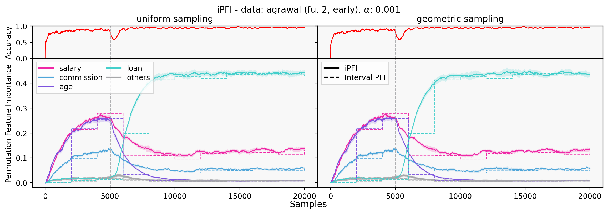
Figure 9: iPFI on agrawal with a function-drift (fu. 2, early) after 5k samples with $\alpha=0.001$ (top) and $\alpha=0.01$ (bottom).

Figure 10: iPFI on agrawal with a function-drift (fu. 2, late) after 15k samples with $\alpha=0.001$ (top) and $\alpha=0.01$ (bottom).

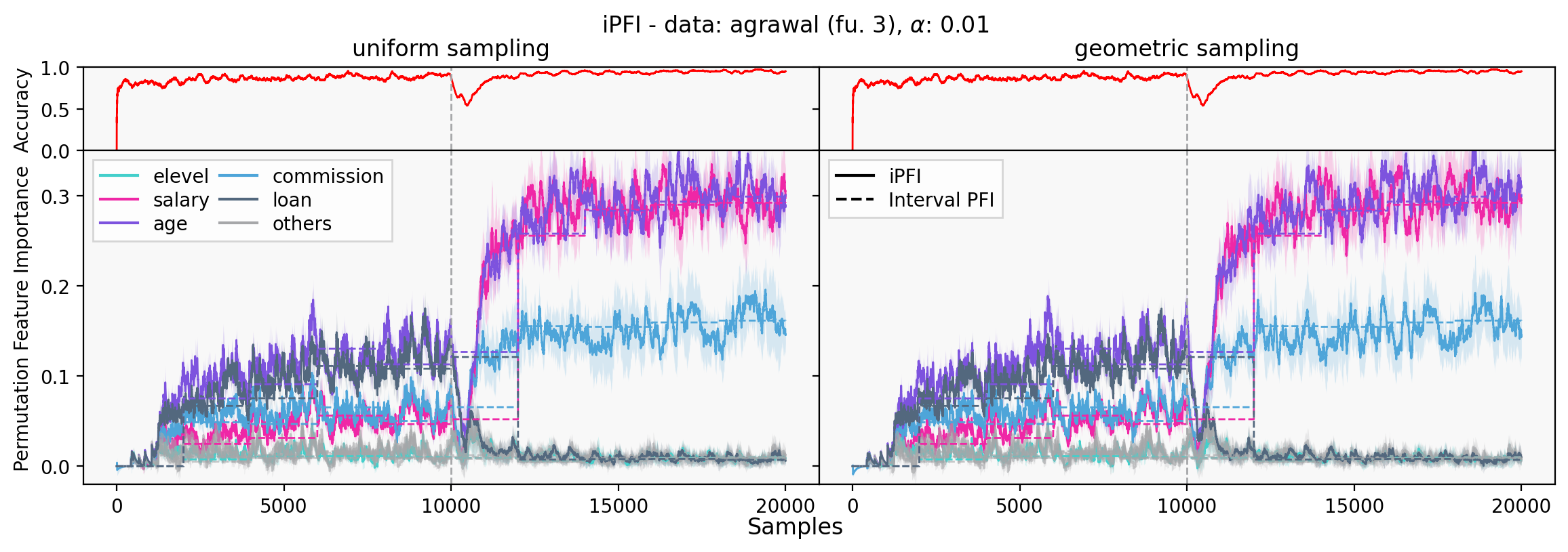
Figure 11: iPFI on agrawal with a function-drift (fu. 3) after 10k samples with $\alpha=0.001$ (top) and $\alpha=0.01$ (bottom).

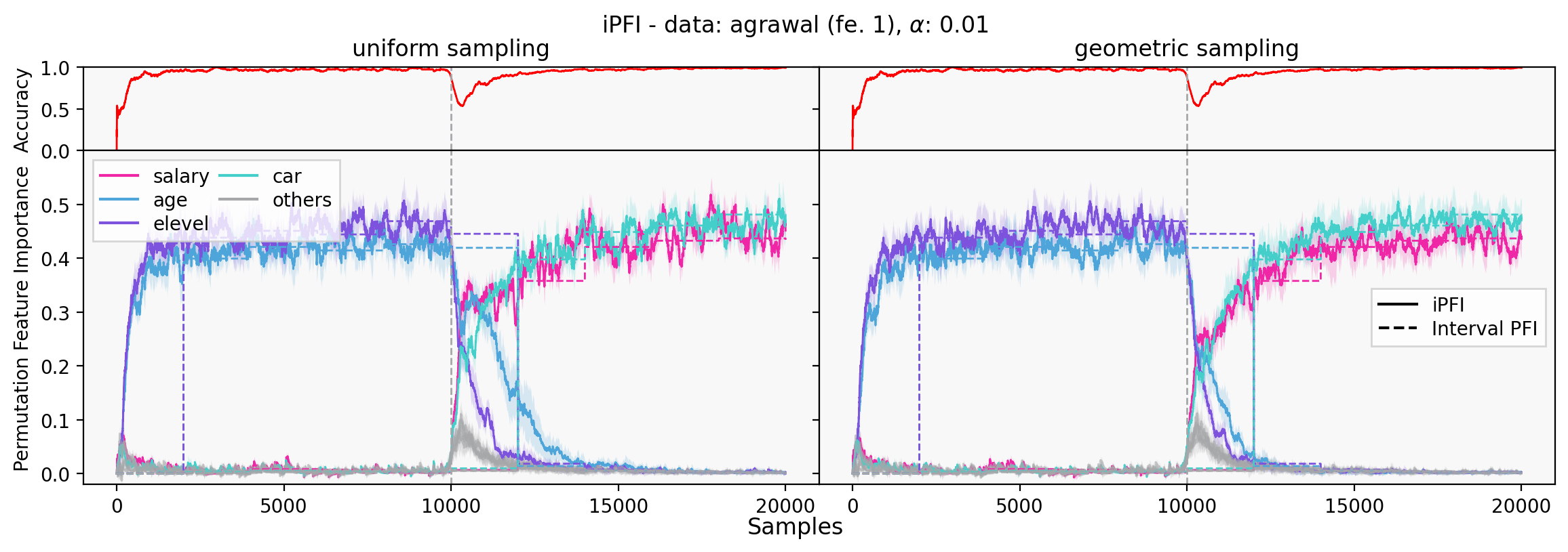
Figure 12: iPFI on agrawal with a feature-drift (fe. 1) after 10k samples with $\alpha=0.001$ (top) and $\alpha=0.01$ (bottom).

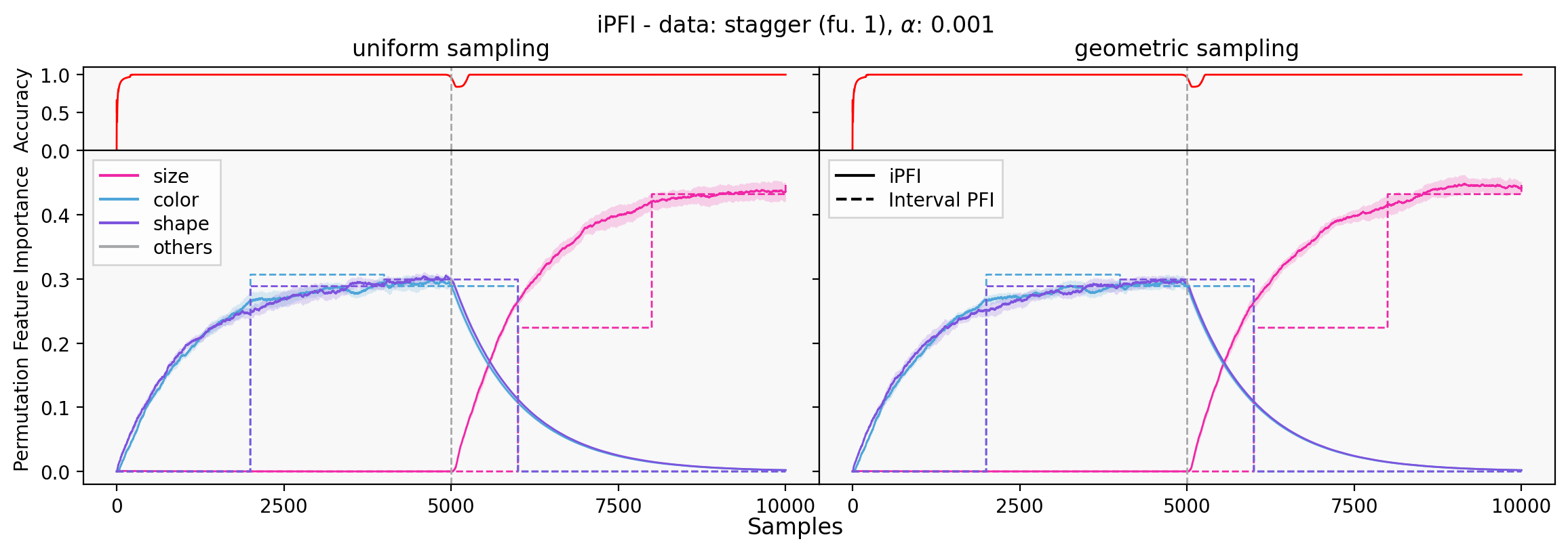
Figure 13: iPFI on stagger with a feature-drift (fu. 1) after 5k samples with $\alpha=0.001$.

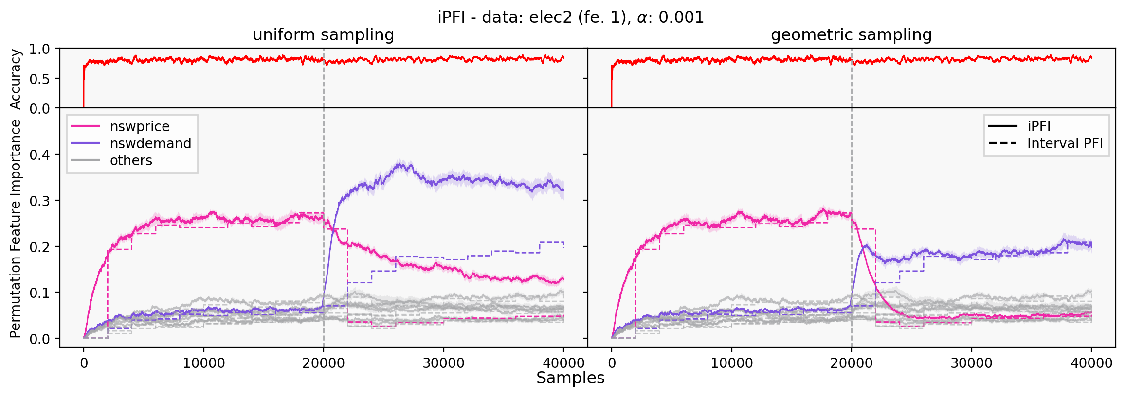
Figure 14: iPFI on elec2 with a sudden feature-drift (fe. 1) (top) and a gradual feature-drift (fe. 1, gradual) (bottom) after 20k samples with $\alpha=0.001$.

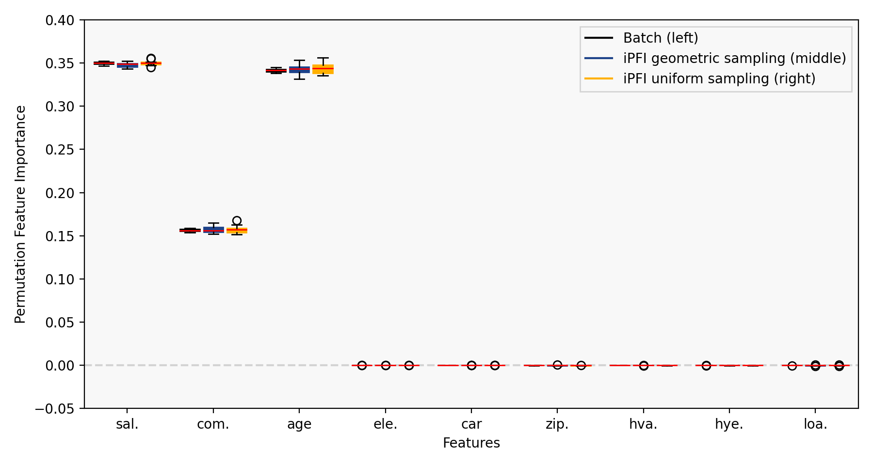
Figure 15: Boxplot of PFI estimates per feature of the agrawal dataset for batch baseline (left), iPFI with geometric sampling (middle), and iPFI with uniform sampling (right) on a pre-trained static LGBM.

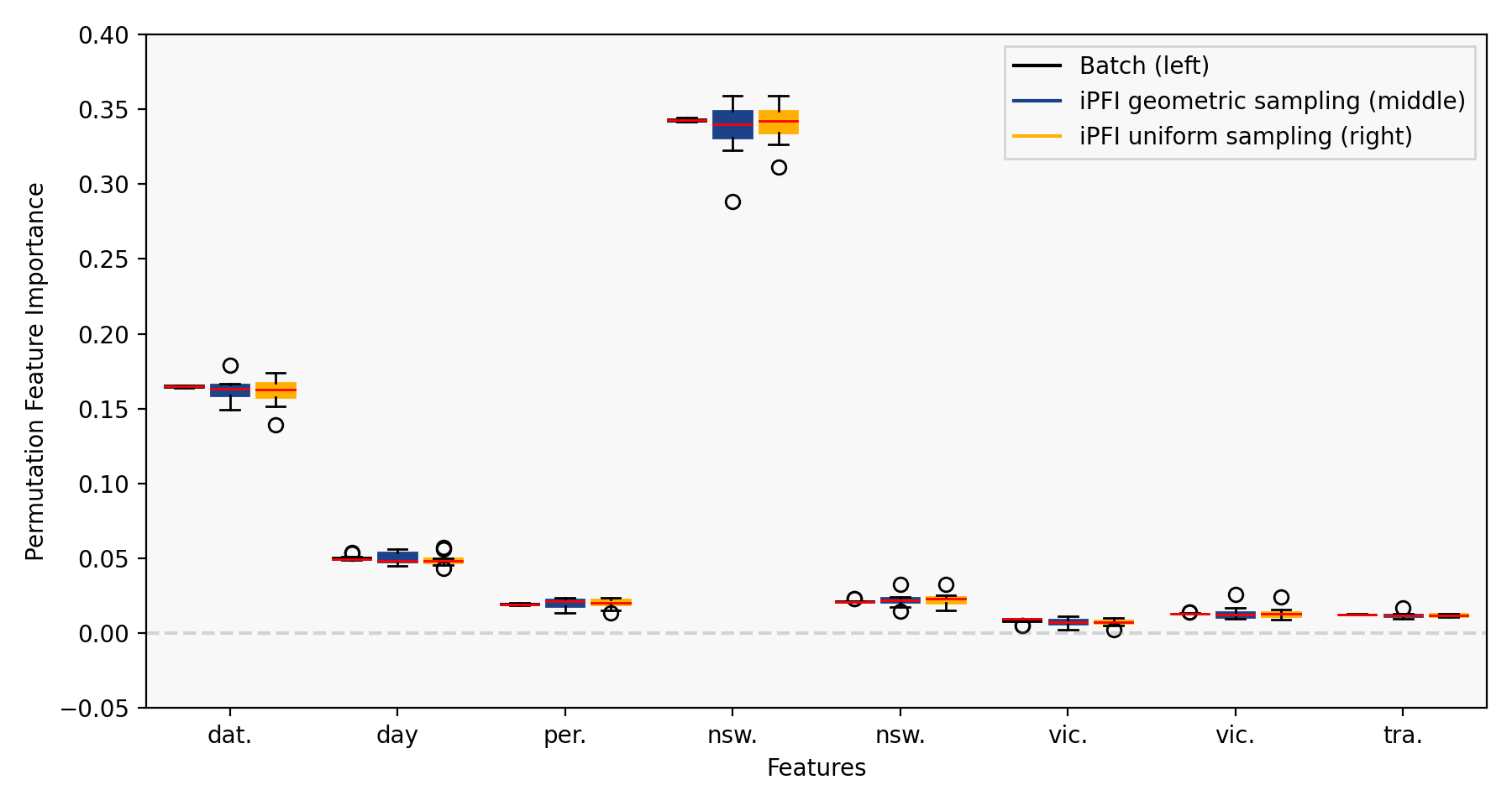
Figure 16: Boxplot of PFI estimates per feature of the elec2 dataset for batch baseline (left), iPFI with geometric sampling (middle), and iPFI with uniform sampling (right) on a pre-trained static LGBM.

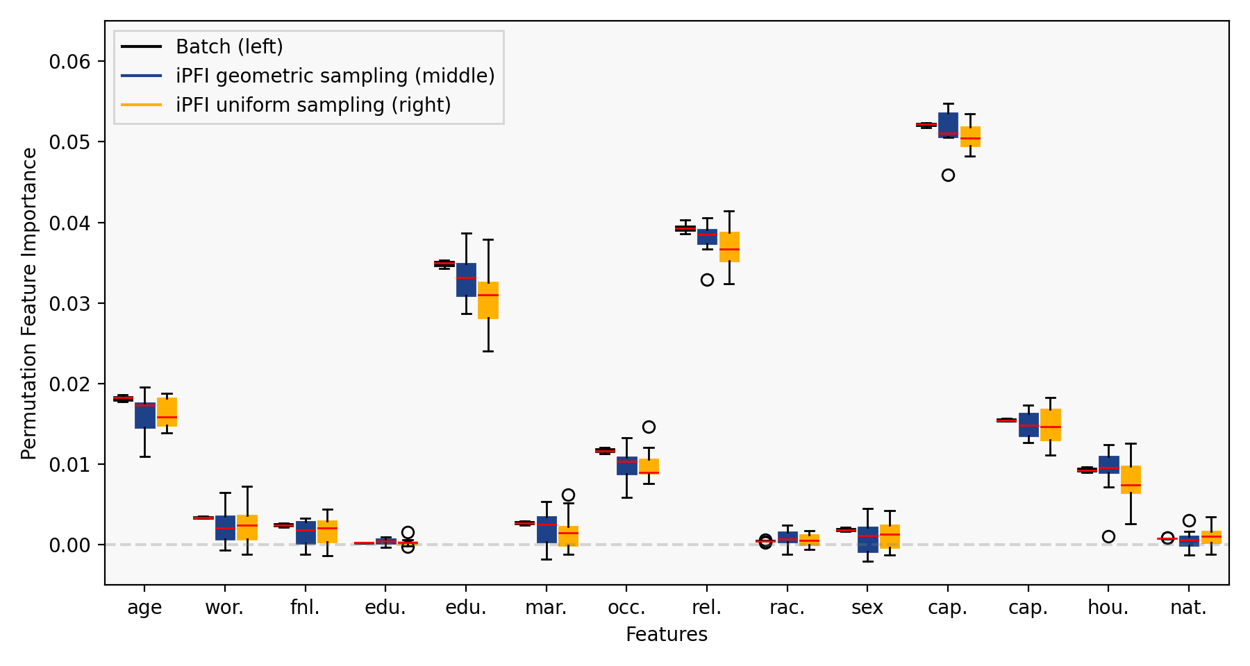
Figure 17: Boxplot of PFI estimates per feature of the adult dataset for batch baseline (left), iPFI with geometric sampling (middle), and iPFI with uniform sampling (right) on a pre-trained static GBT.

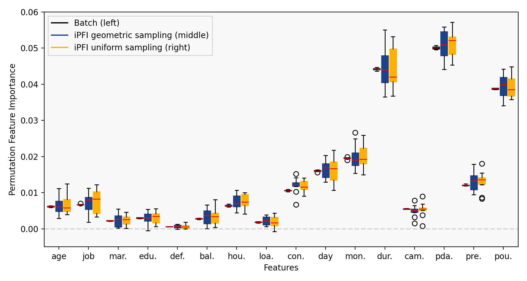
Figure 18: Boxplot of PFI estimates per feature of the bank dataset for batch baseline (left), iPFI with geometric sampling (middle), and iPFI with uniform sampling (right) on a pre-trained static NN.

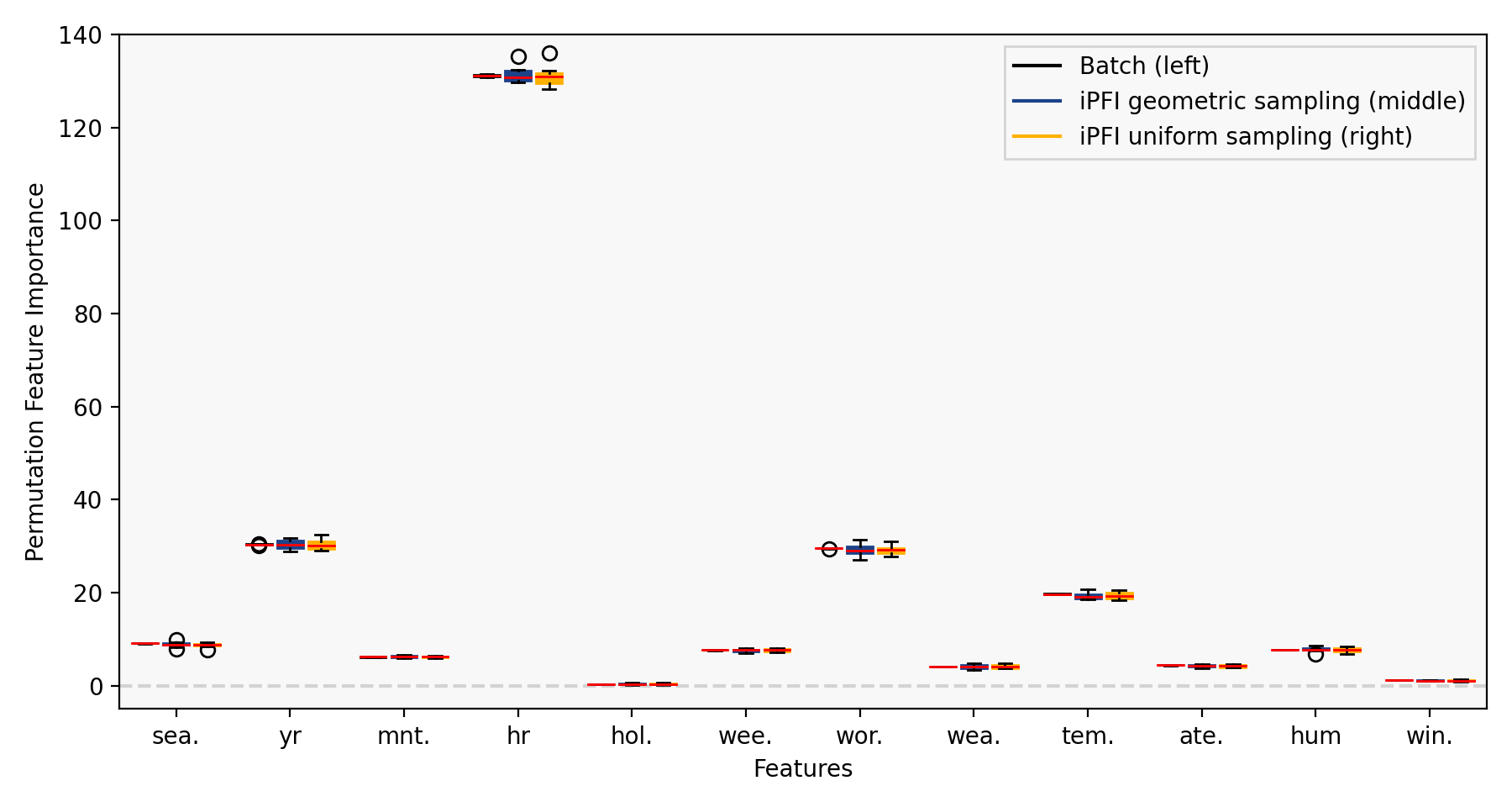
Figure 19: Boxplot of PFI estimates per feature of the bike dataset for batch baseline (left), iPFI with geometric sampling (middle), and iPFI with uniform sampling (right) on a pre-trained static LGBM.

References

- Adadi and Berrada (2018) Adadi, A.; and Berrada, M. 2018. Peeking Inside the Black-Box: A Survey on Explainable Artificial Intelligence (XAI). IEEE Access, 6: 52138–52160.
- Agrawal, Imielinski, and Swami (1993) Agrawal, R.; Imielinski, T.; and Swami, A. 1993. Database Mining: A Performance Perspective. IEEE Transactions on Knowledge and Data Engineering, 5(6): 914–925.
- Bach et al. (2015) Bach, S.; Binder, A.; Montavon, G.; Klauschen, F.; Müller, K.-R.; and Samek, W. 2015. On pixel-wise explanations for non-linear classifier decisions by layer-wise relevance propagation. PloS one, 10(7): e0130140.
- Bahri et al. (2021) Bahri, M.; Bifet, A.; Gama, J.; Gomes, H. M.; and Maniu, S. 2021. Data stream analysis: Foundations, major tasks and tools. Wiley Interdisciplinary Reviews: Data Mining and Knowledge Discovery, 11(3): e1405.
- Barddal et al. (2019) Barddal, J. P.; Enembreck, F.; Gomes, H. M.; Bifet, A.; and Pfahringer, B. 2019. Boosting decision stumps for dynamic feature selection on data streams. Information Systems, 83: 13–29.
- Breiman (2001) Breiman, L. 2001. Random Forests. Machine Learning, 45(1): 5–32.
- Cassidy and Deviney (2014) Cassidy, A. P.; and Deviney, F. A. 2014. Calculating feature importance in data streams with concept drift using Online Random Forest. In 2014 IEEE International Conference on Big Data (Big Data), 23–28.
- Covert and Lee (2021) Covert, I.; and Lee, S.-I. 2021. Improving KernelSHAP: Practical Shapley Value Estimation Using Linear Regression. In Banerjee, A.; and Fukumizu, K., eds., The 24th International Conference on Artificial Intelligence and Statistics (AISTATS 2021), volume 130 of Proceedings of Machine Learning Research, 3457–3465. PMLR.
- Covert, Lundberg, and Lee (2021) Covert, I.; Lundberg, S.; and Lee, S.-I. 2021. Explaining by Removing: A Unified Framework for Model Explanation. Journal of Machine Learning Research, 22(209): 1–90.
- Covert, Lundberg, and Lee (2020) Covert, I.; Lundberg, S. M.; and Lee, S.-I. 2020. Understanding Global Feature Contributions With Additive Importance Measures. In Proceedings of International Conference on Neural Information Processing Systems, 17212–17223.
- Doshi-Velez and Kim (2017) Doshi-Velez, F.; and Kim, B. 2017. Towards a rigorous science of interpretable machine learning. arXiv:1702.08608.
- Fanaee-T and Gama (2014) Fanaee-T, H.; and Gama, J. 2014. Event labeling combining ensemble detectors and background knowledge. Progress in Artificial Intelligence, 2(2): 113–127.
- Feurer et al. (2020) Feurer, M.; van Rijn, J. N.; Kadra, A.; Gijsbers, P.; Mallik, N.; Ravi, S.; Mueller, A.; Vanschoren, J.; and Hutter, F. 2020. OpenML-Python: an extensible Python API for OpenML. arXiv:1911.02490.
- Fisher, Rudin, and Dominici (2019) Fisher, A.; Rudin, C.; and Dominici, F. 2019. All Models are Wrong, but Many are Useful: Learning a Variable’s Importance by Studying an Entire Class of Prediction Models Simultaneously. Journal of Machine Learning Research, 20(177): 1–81.
- Friedman (2001) Friedman, J. H. 2001. Greedy function approximation: A gradient boosting machine. The Annals of Statistics, 29(5): 1189–1232.
- García-Martín et al. (2019) García-Martín, E.; Rodrigues, C. F.; Riley, G.; and Grahn, H. 2019. Estimation of energy consumption in machine learning. Journal of Parallel and Distributed Computing, 134: 75–88.
- Gomes et al. (2017) Gomes, H. M.; Bifet, A.; Read, J.; Barddal, J. P.; Enembreck, F.; Pfharinger, B.; Holmes, G.; and Abdessalem, T. 2017. Adaptive random forests for evolving data stream classification. Machine Learning, 106(9): 1469–1495.
- Gregorutti, Michel, and Saint-Pierre (2017) Gregorutti, B.; Michel, B.; and Saint-Pierre, P. 2017. Correlation and variable importance in random forests. Statistics and Computing, 27(3): 659–678.
- Harries (1999) Harries, M. 1999. SPLICE-2 Comparative Evaluation: Electricity Pricing. Technical report, The University of South Wales.
- Hoeffding (1948) Hoeffding, W. 1948. A Class of Statistics with Asymptotically Normal Distribution. The Annals of Mathematical Statistics, 19(3): 293 – 325.
- Janzing, Minorics, and Bloebaum (2020) Janzing, D.; Minorics, L.; and Bloebaum, P. 2020. Feature relevance quantification in explainable AI: A causal problem. In Proceedings of International Conference on Artificial Intelligence and Statistics, 2907–2916.
- Jethani et al. (2021) Jethani, N.; Sudarshan, M.; Covert, I. C.; Lee, S.-I.; and Ranganath, R. 2021. FastSHAP: Real-time shapley value estimation. In Proceedings of International Conference on Learning Representations.
- Ke et al. (2017) Ke, G.; Meng, Q.; Finley, T.; Wang, T.; Chen, W.; Ma, W.; Ye, Q.; and Liu, T.-Y. 2017. Lightgbm: A highly efficient gradient boosting decision tree. Proceedings of International Conference on Neural Information Processing System, 30.
- Kohavi (1996) Kohavi, R. 1996. Scaling up the Accuracy of Naive-Bayes Classifiers: A Decision-Tree Hybrid. In Proceedings of International Conference on Knowledge Discovery and Data Mining, 202–207.
- König et al. (2021) König, G.; Molnar, C.; Bischl, B.; and Grosse-Wentrup, M. 2021. Relative feature importance. In Proceedings of International Conference on Pattern Recognition, 9318–9325.
- Losing, Hammer, and Wersing (2018) Losing, V.; Hammer, B.; and Wersing, H. 2018. Incremental On-line Learning: A Review and Comparison of State of the Art Algorithms. Neurocomputing, 275: 1261–1274.
- Lundberg et al. (2020) Lundberg, S. M.; Erion, G.; Chen, H.; DeGrave, A.; Prutkin, J. M.; Nair, B.; Katz, R.; Himmelfarb, J.; Bansal, N.; and Lee, S.-I. 2020. From local explanations to global understanding with explainable AI for trees. Nature Machine Intelligence, 2(1): 56–67.
- Lundberg and Lee (2017) Lundberg, S. M.; and Lee, S.-I. 2017. A Unified Approach to Interpreting Model Predictions. In Proceedings of International Conference on Neural Information Processing Systems, 4768–4777.
- Molnar et al. (2020) Molnar, C.; König, G.; Bischl, B.; and Casalicchio, G. 2020. Model-agnostic Feature Importance and Effects with Dependent Features–A Conditional Subgroup Approach. arXiv:2006.04628.
- Montiel et al. (2020) Montiel, J.; Halford, M.; Mastelini, S. M.; Bolmier, G.; Sourty, R.; Vaysse, R.; Zouitine, A.; Gomes, H. M.; Read, J.; Abdessalem, T.; and Bifet, A. 2020. River: machine learning for streaming data in Python. arXiv:2012.04740.
- Moro, Cortez, and Laureano (2011) Moro, S.; Cortez, P.; and Laureano, R. 2011. Using Data Mining for Bank Direct Marketing: An Application of the CRISP-DM Methodology. Proceedings of the European Simulation and Modelling Conference.
- Muschalik et al. (2022) Muschalik, M.; Fumagalli, F.; Hammer, B.; and Hüllermeier, E. 2022. Agnostic Explanation of Model Change based on Feature Importance. KI - Künstliche Intelligenz.
- Nahmias and Olsen (2015) Nahmias, S.; and Olsen, T. L. 2015. Production and operations analysis. Waveland Press.
- Pedregosa et al. (2011) Pedregosa, F.; Varoquaux, G.; Gramfort, A.; Michel, V.; Thirion, B.; Grisel, O.; Blondel, M.; Prettenhofer, P.; Weiss, R.; Dubourg, V.; Vanderplas, J.; Passos, A.; Cournapeau, D.; Brucher, M.; Perrot, M.; and Duchesnay, E. 2011. Scikit-learn: Machine Learning in Python. Journal of Machine Learning Research, 12: 2825–2830.
- Rényi (1961) Rényi, A. 1961. On measures of entropy and information. In Proceedings of the Fourth Berkeley Symposium on Mathematical Statistics and Probability, Volume 1: Contributions to the Theory of Statistics, 547–562.
- Ribeiro, Singh, and Guestrin (2016) Ribeiro, M. T.; Singh, S.; and Guestrin, C. 2016. ”Why Should I Trust You?”: Explaining the Predictions of Any Classifier. In Proceedings of International Conference on Knowledge Discovery and Data Mining, San Francisco, 1135–1144.
- Schlimmer and Granger (1986) Schlimmer, J. C.; and Granger, R. H. 1986. Incremental Learning from Noisy Data. Mach. Learn., 1(3): 317–354.
- Selvaraju et al. (2017) Selvaraju, R. R.; Cogswell, M.; Das, A.; Vedantam, R.; Parikh, D.; and Batra, D. 2017. Grad-cam: Visual explanations from deep networks via gradient-based localization. In Proceedings of the IEEE international Conference on Computer Vision, 618–626.
- Turkay et al. (2018) Turkay, C.; Pezzotti, N.; Binnig, C.; Strobelt, H.; Hammer, B.; Keim, D. A.; Fekete, J.-D.; Palpanas, T.; Wang, Y.; and Rusu, F. 2018. Progressive Data Science: Potential and Challenges. arXiv:1812.08032.
- Vitter (1985) Vitter, J. S. 1985. Random Sampling with a Reservoir. ACM Transactions on Mathematical Software, 11(1): 37–57.
- Wastensteiner et al. (2021) Wastensteiner, J.; Weiss, T. M.; Haag, F.; and Hopf, K. 2021. Explainable AI for Tailored Electricity Consumption Feedback: An Experimental Evaluation of Visualizations. In Quammah, A. E., ed., European Conference on Information Systems (ECIS 2021), volume 55.
- Yuan, Pfahringer, and Barddal (2018) Yuan, L.; Pfahringer, B.; and Barddal, J. P. 2018. Iterative subset selection for feature drifting data streams. In Proceedings of the 33rd Annual ACM Symposium on Applied Computing, 510–517.
Acknowledgments
We gratefully acknowledge funding by the Deutsche Forschungsgemeinschaft (DFG, German Research Foundation): TRR 318/1 2021 – 438445824.
Technical Supplement