Elementary excitations of dipolar Tonks-Girardeau droplets

Abstract

One-dimensional bosonic gas with strong contact repulsion and attractive dipolar interactions may form a quantum droplet with flat-top density profile. Employing effective, hydrodynamic description of the system, we study elementary excitations characterizing response of a droplet to small perturbation. The excitation spectrum consists of two families: phononic-like excitations inside droplets and the scattering modes. Analysis within the linearized regime is supplemented with the full, nonlinear dynamics of small perturbations. Our study focuses mainly on the regime of infinite contact repulsion and tight transversal harmonic confinement, where there are analytic formulas for the density profiles. Moreover, we propose a simplified analytic ansatz suitable to work also outside this regime, provided the gas is in the deep flat-top region of density profiles.

I Introduction

Quantum droplets are a prime example that the mean-field (MF) description may fail even for weakly interacting Bose gas  Petrov (2015); Lima and Pelster (2012, 2011); Böttcher et al. (2021). The MF approach predicts an unstable weakly interacting system, where the corresponding attractive and repulsive contributions nearly cancel each other. This gives way to the enhanced role of zero-point energy fluctuations, usually named the Lee-Huang-Yang (LHY) term Lee et al. (1957), stabilising the emerging droplet. Quantum liquids, however, are more robust in lower dimensions due to the increased quantum fluctuations Petrov and Astrakharchik (2016a); Edler et al. (2017a); Astrakharchik and Malomed (2018); Zin et al. (2018); Ilg et al. (2018); Rakshit et al. (2019); Edmonds et al. (2020); Morera et al. (2020, 2021); Guijarro et al. (2022); Natale et al. (2022).

Particularly, in 1D, quantum droplets have been recently theoretically studied for strongly correlated systems with non-local interactions both in continuum and in the presence of an optical lattice Ołdziejewski et al. (2020); De Palo et al. (2021, 2022); Morera et al. (2022). In the former case, a quantum liquid obeys the so-called Lieb-Liniger Gross-Pitaevski Kopyciński et al. (2022a) equation (LLGPE) that, in the limit of weakly interacting gas, reduces to a standard Gross-Pitaevski equation with the 1D LHY term for short-range interaction. Importantly, in all interaction regimes in 1D, quantum droplets exhibit qualitatively the same ground-state features such as being ultradilute self-bound objects (negative energy for an untrapped state) and having constant chemical potential marked by the flat-top density profile Böttcher et al. (2021).

A hallmark of one-dimensional quantum systems with attractive forces is a transition between droplets and solitons Edler et al. (2017b); Tylutki et al. (2020); Ołdziejewski et al. (2020). Both are bound states, present for an arbitrary number of particles for different interaction regimes. Namely, a droplet solution appears when short-range repulsion prevails over long-range attraction, contrary to the bright soliton case. Although quantum droplets in 1D exhibit a characteristic flat-top density profile for greater numbers of particles, for smaller systems, one can only distinguish between a bright soliton and a droplet by studying their excitations spectrum. This is motivated by the fact, that in a one-dimensional Bose system at least in case without LHY corrections, there are no collective modes in a bright soliton – there are continuum modes solely Castin and Herzog (2001). In contrast, the excitation spectrum of a droplet supports small-amplitude collective excitations Tylutki et al. (2020). Moreover, the excitation spectrum differs between 1D and 3D droplets, for the latter supports both bulk and surface modes Bulgac (2002); Petrov (2015).

Little is known, however, how the above picture changes by introducing strong correlations between the particles. For instance, for repulsive contact interaction, one can experimentally show that while tuning from the weakly to the strongly interacting regime via a magnetic Feshbach resonance, the dispersion changes dramatically by emerging holelike excitations absent for higher dimension and weaker interactions Meinert et al. (2015). The recent progress in preparing a bosonic one-dimensional quantum gas of dysprosium Kao et al. (2021) warrants further studies on the exact nature of excitations in one-dimensional systems with simultaneously present attraction and repulsion.

In this work, we investigate the excitation spectrum of a one-dimensional strongly correlated dipolar Bose gas. The complementary problem of solitonic excitations in such system was studied in Kopyciński et al. (2022b). The system is described with an effective, hydrodynamic approach introduced in earlier works Ołdziejewski et al. (2020); Kopyciński et al. (2022a). The problem poses a serious challenge in solving because of the presence of non-local dipolar interaction and a quite intricate form of short-range contribution. We thus first focus on a analytical regime of fermionised bosons and vanishing range of dipolar forces. We find a qualitative agreement with previous results about weakly interacting Bose-Bose mixtures Tylutki et al. (2020) further confirming robustness of quantum droplets in lower dimensions. Next, we generalise our observations to the full problem.

Let us outline the most important findings of our paper. We analyze the excitation spectrum of dipolar quantum droplets by solving the Bogoliubov-de Gennes (BdG) equations. This is done with an emphasis on regimes, where this complex problem simplifies and analytical treatment is at hand. In particular, in the regime of strong contact interactions and short range of dipolar forces, the density profile of a droplet can be found analytically. We thoroughly study this regime obtaining the expression for the droplet energy and characterize the excitation spectrum. What is more, insights from that analysis motivate a very simple rectangular ansatz for the density profiles of droplets. Within approximation of such ansatz, we derive simple and useful formulas for the droplet width and energy. Moreover, we obtain expressions for the excitation spectrum and the number of phononic bound modes that a droplet can exhibit. The ansatz works also outside the aforementioned regime of strong contact interactions and short-ranged dipolar interactions as long as the droplet’s shape is dominated by the bulk, flat-top part. In addition to the study of excitations within the framework of BdG equations, we numerically analyze the response to the initial perturbation in the full, nonlinear dynamics.

The paper is organized as follows. In Sec. II we introduce the most important features of the system under study. We briefly describe the effective dipolar interactions in one dimension and the hydrodynamic description of strongly interacting Bose gas. This is followed by the analysis of the ground state of the system. In particular, we specify the regime, for which the density profile of the droplet can be found exactly and introduce the rectangular ansatz for the density profiles. After that, in Sec. III we present the results for the excitation spectrum obtained from the solution of BdG equations. In Sec. IV we broaden this analysis by studying the response to initial perturbation in dynamics given by the nonlinear, hydrodynamic equation. Finally, in Sec. V we give a summary of results presented in the paper.

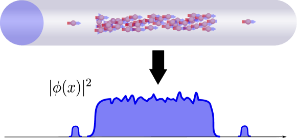
Figure 1: We study a gas of atoms trapped in a quasi-1D tube, with dipole moments polarized. Here, we present head-to-tail configuration that leads to attractive interactions between dipoles. Exciting a quantum droplet state may result in an emission of the matter waves.

II Model

We consider a system of $N$ bosonic atoms with mass $m$ confined to a quasi-one-dimensional geometry, i.e. we assume a very tight harmonic trap with frequency $\omega_{\perp}$ in the $y$ and $z$ directions, but particles are unconfined in the $x$ direction. The atoms interact via repulsive contact potential and attractive dipolar forces. As shown in Fig. 1, the atomic dipole moments, $\bm{\mu}_{D}$ are aligned with an external magnetic field so that the interaction is attractive. We assume that, the trap in the perpendicular $y$ and $z$ directions is so steep, that the motion in these directions is frozen, i.e. atoms occupy the ground state Gaussians. In this situation, one can integrate out the spatial $y$ and $z$ degrees of freedom to obtain an effective model describing the system restricted to $x$ direction only.

This procedure leads to the effective 1D inter-particle interaction potential

$$V(x-x^{\prime})=g\delta(x-x^{\prime})-g_{\text{dd}}V_{\text{dd}}^{\sigma}(x-x^{\prime}),\qquad g,g_{\text{dd}}>0.$$ (1)

The first term expresses the short-range interaction, with the interaction coefficient $g$. The second term, coming from the long-range dipolar potential takes the form Deuretzbacher et al. (2010)

$$V_{\text{dd}}^{\sigma}(x-x^{\prime})=\frac{v(\frac{x-x^{\prime}}{\sigma})}{\sigma},\quad v(u)=\frac{1}{4}\bigg{(}-2|u|+\sqrt{2\pi}(1+u^{2})e^{u^{2}/2}\text{Erfc}(|u|/\sqrt{2})\bigg{)},$$ (2)

where $g_{\text{dd}}=\frac{\mu_{0}\mu_{D}^{2}(3\cos^{2}\theta-1)}{4\pi\sigma^{2}}$, with $\theta$ denoting the angle between orientation of the dipoles and $x$ axis. The full dipolar potential reduced to 1D, i.e. $V_{\text{dd}}^{\sigma}(x)$ is finite at the origin and it has the characteristic effective range that depends on the oscillatory length of the transverse confinement $\sigma=\sqrt{\frac{\hbar}{m\omega_{\perp}}}$. In particular, when transverse trap is getting tighter with $\omega_{\perp}\to\infty$, then $\sigma\to 0$, and the quasi-1D dipolar potential tends to the delta function $V_{\text{dd}}^{\sigma}(x)\to\delta(x)$.

In this paper, we wish to study the regime of strong contact interactions. That is why we cannot simply adapt the standard mean-field approach typically used for the description of 1D dipolar quantum droplets, i.e. GP equation supplemented with LHY term Böttcher et al. (2021). Instead, we turn to the effective, hydrodynamic equation described earlier in Kopyciński et al. (2022a); Ołdziejewski et al. (2020), which is based on the density field $\rho(x)$ and the velocity field $v(x)$. Briefly, we use local density approximation and locally, the energy of contact interactions is expressed with the exact ground state energy function $E_{\text{LL}}(\gamma)$ from the Lieb-Liniger model Lieb and Liniger (1963); Lieb (1963)

$$E_{\text{LL}}(\gamma)=\frac{\hbar^{2}}{2m}N\rho^{2}e_{\text{LL}}(\gamma)$$ (3)

where $\gamma=\frac{m}{\hbar^{2}}\frac{g}{\rho}$ with $\rho$ denoting density of the gas. In order to account for the density slowly varying in space, we promote the parameter $\gamma$ to a function of position $\gamma\to\gamma(x)=\frac{m}{\hbar^{2}}\frac{g}{\rho(x)}$. The function $e_{\text{LL}}(\gamma)$ present in (3) has no known compact analytical form but there exist accurate and handy approximations to it Lang et al. (2017); Ristivojevic (2019); Prolhac (2017). Energy associated with the dipolar interactions is approximated in the standard mean-field way. Precisely, we assume that the dipolar interaction couples densities in different positions and neglect contributions from higher order correlations between atoms. Such an approximation is expected to work when the range of the dipolar interactions $\sigma$ is much larger than the average interparticle spacing defining the fermionization length scale Ołdziejewski et al. (2020). The full energy functional reads

$$E[\phi] =N\int dx\Big{[}\frac{\hbar^{2}}{2m}\left|\frac{\partial\phi}{\partial x}\right|^{2}+\frac{N^{2}\hbar^{2}}{2m}|\phi|^{6}e_{\rm LL}\bigg{(}\frac{gm}{\hbar^{2}N|\phi|^{2}}\bigg{)}+$$ (4)

$$-\frac{1}{2}Ng_{\text{dd}}\int dx^{\prime}V_{\text{DD}}^{\sigma}(x-x^{\prime})|\phi(x)|^{2}|\phi(x^{\prime})|^{2}\Big{]}.$$

The normalized complex field $\phi(x)$ is directly related to two hydrodynamic fields $\rho(x)$ and $v(x)$ via relation

$$\phi(x)=\sqrt{\rho(x)/N}e^{i\varphi(x)},$$ (5)

where $\hbar\partial_{x}\varphi(x)=m\,v(x)$. Applying variational principle to the energy functional (4) leads to

$$i\frac{\partial\phi(x,t)}{\partial t} =-\frac{1}{2}\frac{\partial^{2}\phi(x,t)}{\partial x^{2}}+\mu_{\rm LL}\left[N|\phi(x,t)|^{2}\right]\,\phi(x,t)$$

$$-g_{\text{dd}}N\int dx^{\prime}V_{\text{dd}}^{\sigma}(x-x^{\prime})|\phi(x^{\prime},t)|^{2}\phi(x,t),$$ (6)

where, for brevity, we use $\hbar=m=1$. In the equation above we have introduced a functional defining local chemical potential in the Lieb-Liniger model Lieb and Liniger (1963)

$$\mu_{\rm LL}\left[N|\phi|^{2}\right]=\frac{1}{2}N^{2}|\phi|^{4}\left(3e_{\rm LL}\left(\frac{g}{N|\phi|^{2}}\right)-\frac{g}{N|\phi|^{2}}e^{\prime}_{\rm LL}\left(\frac{g}{N|\phi|^{2}}\right)\right).$$ (7)

The stationary version of Eq. (II) reads

$$\mu\,\phi_{0}(x)=-\frac{1}{2}\frac{\partial^{2}\phi_{0}(x)}{\partial x^{2}}+\mu_{\rm LL}\left[N|\phi_{0}(x)|^{2}\right]\,\phi_{0}(x)-g_{\text{dd}}N\int dx^{\prime}V_{\text{dd}}^{\sigma}(x-x^{\prime})|\phi_{0}(x^{\prime})|^{2}\phi_{0}(x),$$ (8)

where $\mu$ in turn is the chemical potential of the stationary solution $\phi_{0}$. Let us note that a simplified version of Eq. (8), but with an approximate expression for $e_{\text{LL}}(\gamma)$, was studied before in Ołdziejewski et al. (2020). Importantly, for strong short range interaction and sufficiently weak dipolar potential, the ground state of Eq. (4) is a quantum droplet, with characteristic flat-top density profile Ołdziejewski et al. (2020).

In general, Eq. (8) does not have an analytical solution and one must use numerical methods such as imaginary time evolution to solve it. However, there are some special cases, where the equation simplifies and becomes exactly solvable, yielding closed analytical expressions for density profiles of quantum droplets. In this paper, we will mainly focus on these regimes, as the analytical solution allows for a detailed analysis of elementary excitations and comparison with approximate ansatz solutions.

II.1 Analytical regime: $g\to\infty$ and $\sigma\to 0$

In the limit of infinitely strong contact repulsion $g\to\infty$ (fermionization regime with $e_{\text{LL}}(\gamma\to\infty)=\pi^{2}/3$) and short-range dipolar interactions $\sigma\to 0$ the Eq. (II) can be significantly simplified and one finds its exact analytical solutions. Therefore, hereafter we refer to this regime as analytical regime. In this regime Eq. (II) reduces to

$$\mu\phi=-\frac{1}{2}\frac{\partial^{2}\phi}{\partial x^{2}}+\frac{\pi^{2}N^{2}}{2}|\phi|^{4}\phi-g_{\text{dd}}N|\phi|^{2}\phi,$$ (9)

which was studied also in Baizakov et al. (2009). In this special limit the energy functional simplifies to

$$E[\phi] =N\int dx\Big{[}\frac{1}{2}\left|\partial_{x}\phi\right|^{2}+\frac{N^{2}}{2}\frac{\pi^{2}}{3}|\phi|^{6}-\frac{1}{2}Ng_{\text{dd}}|\phi(x)|^{4}\Big{]}.$$ (10)

Note, that the resulting equation contains two competing nonlinear terms, that are different than the nonlinearities appearing for weak interactions only Lima and Pelster (2012).

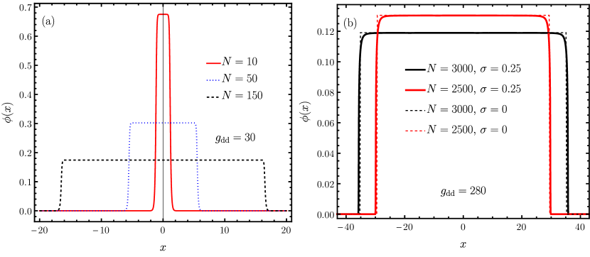
Figure 2: Panel (a): Analytical solutions (11) in the fermionization regime, with range of dipolar interactions $\sigma=0$ for different particle numbers $N$ and fixed $g_{\text{dd}}=30$. The droplet becomes wider with increasing $N$. Moreover, the density profiles become dominated by the bulk, flat-top part and approach a rectangular shape. Panel (b): Fermionization regime with fixed $g_{\text{dd}}=280$. Numerical solutions of Eq. (8) with finite dipolar range $\sigma=0.25$ (solid lines) together with $\sigma=0$ analytical solution (11) to the Eq. (9) (dashed lines). The differences are small and visible only close to the edges of the droplet. Parameter $\kappa\approx 10.6$ fulfills the condition defining the range of applicability of (9). The atom number is so large that analytical solutions (11) are very close to the rectangular ansatz (17).

The ground state of Eq.  (10) has been derived in the context of the nonlinear optics Pushkarov et al. (1979), and it reads

$$\phi^{\infty}(x)=\sqrt{\frac{\sqrt{3}g_{\text{dd}}}{2\pi\eta}}\frac{\tanh(\eta)}{\sqrt{1+\text{sech}(\eta)\,\cosh(x/a)}},$$ (11)

where

$$\eta=\frac{\pi N}{\sqrt{3}}\qquad a=\frac{\pi}{\sqrt{3}g_{\text{dd}}\tanh(\eta)}.$$ (12)

Plots of the solution (11) for some exemplary parameters are presented in Fig. 2(a). We also derived the total energy (10) of the ground state solution (11), in terms of its three contributions, corresponding to the kinetic energy of the envelope $E_{\rm kin}$, the Tonks-Girardeau energy $E_{\rm TG}$ and the dipolar $E_{\rm dip}$ energy. The explicit formulas are

$$E^{\infty}_{\rm kin}=\frac{3\sqrt{3}}{16\pi^{3}}g_{\text{dd}}^{2}\tanh\eta\Bigg{(}-\frac{\eta}{\cosh\eta\sinh\eta}+1\Bigg{)}$$ (13)

$$E^{\infty}_{\rm TG}=\frac{3\sqrt{3}}{16\pi^{3}}g_{\text{dd}}^{2}\tanh\eta\Bigg{(}(2+\text{sech}^{2}\eta)\eta\coth\eta-3\Bigg{)}$$ (14)

$$E^{\infty}_{\rm dip}=-\frac{12\sqrt{3}}{16\pi^{3}}\pi^{3}\tanh\eta\Bigg{(}\eta\coth\eta-1\Bigg{)}.$$ (15)

In the limit of large number of atoms one obtains a simple expression for the total energy (see Fig. 3 for comparison).

$$E^{\infty}=E^{\infty}_{\rm kin}+E^{\infty}_{\rm TG}+E^{\infty}_{\rm dip}\approx-\frac{3g_{\text{dd}}^{2}}{8\pi^{2}}N+\frac{3\sqrt{3}g_{\text{dd}}^{2}}{8\pi^{3}}.$$ (16)

Note that the $N$-independent term in one dimension can be interpreted as surface tension energy. It contains contribution from all types of energies. Its precise value may be useful for study of the phenomena related to fragmentation of droplets De Palo et al. (2022), as it gives the amount of energy required to split a droplet into two smaller ones.

Before further analysis, let us comment on assumptions leading to Eq. (9). While it is clear that infinitely strong contact interactions are physically reasonable Kinoshita et al. (2004); Paredes et al. (2004), the zero-range limit of dipolar interactions $\sigma\to 0$ may appear suspicious. Indeed, one of the assumptions leading to the approximate, hydrodynamic equation (8) corresponds to a range of the dipolar interactions much larger than the average interparticle spacing $d$. However, interparticle spacing does not enter Eq. (8) explicitly. Therefore, one can find a regime with finite $\sigma$, where the characteristic width of the droplet $W$ is much larger than the range of the dipolar interactions $\sigma$. At the same time, this regime is characterized by $\sigma$ much larger than the average interparticle spacing approximately given by $W/N$. We observe that in such a regime, given by the condition $W\gg\sigma\gg W/N$, one can perform the limit $\sigma\to 0$ in Eq. (8) obtaining roughly the same density profile as compared to the one with finite dipolar range $\sigma$. We confirm that on Fig. 2(b). Later in the text, we estimate width of the droplets as $W=2\pi^{2}N/3g_{\text{dd}}$, hence we can write a condition for reliability of Eq. (4) in terms of parameters of our model in the following way $N\gg\kappa\gg 1$, where $\kappa:=3g_{\text{dd}}\sigma/2\pi^{2}$.

The plots presented in Fig. 2(b) suggests yet another approximation, which will be discussed in the next section.

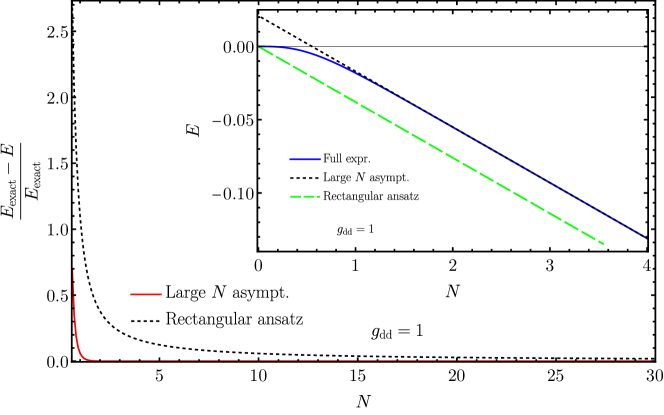
Figure 3: Analytical regime: energy differences between exact energy $E^{\infty}$ and its large $N$ asymptotics (the right hand side of Eq. (16)) and the energy (34) of the rectangular ansatz approximation with fixed $g_{\text{dd}}=1$. The differences are negligible for large enough $N$. Inset: Comparison between the exact energy $E^{\infty}$ together with large $N$ asymptotics and rectangular ansatz formula (34). Dipolar attraction is fixed at $g_{\text{dd}}=1$.

II.2 Rectangular ansatz for the ground state density

Looking at Fig. 2(a) one can notice that when $N$ becomes larger and larger, the solution (11) starts to resemble a rectangle. This motivates us to introduce the following, very simple ansatz

$$\phi_{W}(x)=\frac{1}{\sqrt{W}}\text{rect}(x/W),$$ (17)

where the width $W$ is the only parameter of the ansatz. Although we motivate it mainly by the shape of solutions in the analytical regime, we present results for more general case $g\neq\infty$ and $\sigma\neq 0$. In principle, flat-top shapes resembling rectangle may appear outside the range of parameters for which (8) is exactly solvable. We plug our ansatz to the energy functional Eq. (8) and minimize energy with respect to $W$. Additionally, we neglect term involving $\frac{d\phi}{dx}$, in the same spirit as neglecting the kinetic energy in the Thomas-Fermi approximation. Namely, in the number of parameters we checked that the kinetic energy is much smaller than interaction energy, stemming from the other two terms. This can be confirmed in the analytical regime. The asymptotic form of the kinetic energy (13) becomes $N$-independent there, and thus its contribution to the whole energy (16) is negligible for large $N$. Moreover, to simplify the integral involving dipolar potential, we assume that $W\gg\sigma$. Under these assumptions, we look for the width $W$ minimizing energy

$$\frac{dE}{dW}=\frac{1}{2}N^{3}\Bigg{[}-\frac{2}{W^{3}}e_{\text{LL}}\Big{(}\frac{gW}{N}\Big{)}+\frac{1}{W^{3}}\frac{gW}{N}e_{\text{LL}}^{\prime}\Big{(}\frac{gW}{N}\Big{)}\Bigg{]}+g_{\text{dd}}\frac{N^{2}}{2W^{2}}=0.$$ (18)

The equation above may be formulated in a compact form

$$\frac{1}{\gamma_{W}}\big{(}2e_{\text{LL}}(\gamma_{W})-\gamma_{W}e_{\text{LL}}^{\prime}(\gamma_{W})\big{)}=g_{\text{dd}}/g,$$ (19)

with optimal $W$ hidden in $\gamma_{W}:=gW/N$. From properties of the $e_{\text{LL}}(\gamma)$ function we observe that this equation has a solution only if $g_{\text{dd}}/g<1$, and therefore we expect flat-top solutions only if contact repulsive interactions are stronger than dipolar attraction $g>g_{\text{dd}}$. This is in agreement with previous observations Ołdziejewski et al. (2020); Edler et al. (2017b) suggesting soliton-droplet crossover near $g\approx g_{\text{dd}}$. Additionally, we may calculate the corresponding chemical potential and energy in the rectangular approximation

$$\mu=\mu_{\text{LL}}[N/W]-g_{\text{dd}}\frac{N}{W},\qquad E=\frac{N^{3}}{2W^{2}}e_{\text{LL}}(\gamma_{W})-\frac{N^{2}g_{\text{dd}}}{2W}.$$ (20)

In the limit $g\to\infty$ equation (19) becomes exactly solvable, leading to the explicit formulas for the droplet width

$$W=\frac{2\pi^{2}N}{3g_{\text{dd}}},$$ (21)

the chemical potential and the energy

$$\mu_{W}=-\frac{3g_{\text{dd}}^{2}}{8\pi^{2}},\qquad E_{W}=-\frac{3g_{\text{dd}}^{2}N}{8\pi^{2}}.$$ (22)

In the analytical regime we can directly compare rectangular ansatz energy to the exact expressions. From comparison of Eqs. (16) and (22), we see that rectangular ansatz gives correct value of the term proportional to $N$ but neglects $N-$ independent constant corresponding to surface tension energy. This is in agreement with our initial assumption of large $N$. Additional results in this approach, for energy differences, are presented in Fig. 3.

The rectangular ansatz leads to simple analytic formulas characterizing parameters of a droplet. In the remaining part of the paper we use it further to derive and understand the elementary excitations in the system.

III Elementary excitations

The main goal of this paper is to study excitations of 1D dipolar droplets. Elementary excitations govern their low-energy dynamics, characterize the response to small perturbations and can be used to study the low-temperature thermodynamics. To access elementary excitations and energies, we linearize our equations of motion (II). This procedure, on a formal level, is equivalent to the standard Bogoliubov-de Gennes (BdG) framework applied to nonlinear Schrodinger-like equations Castin (2001). In general, we consider a stationary solution $\phi_{0}(x)$ to the Eq. (II) and wish to characterize a response to some small perturbation of that field. We consider the following, standard ansatz for the perturbed time-dependent field

$$\phi(x,t)=\Big{(}\phi_{\text{0}}(x)+\delta\phi(x,t)\Big{)}e^{-i\mu t},$$ (23)

where $\mu$ is the chemical potential of stationary solution $\phi_{0}(x)$ and the small dynamical perturbation is assumed in the form Pitaevskii and Stringari (2016); Castin (2001)

$$\delta\phi(x,t)=u(x)e^{-i\epsilon t}+v^{*}(x)e^{i\epsilon t}$$ (24)

where the functions $u(x)$ and $v(x)$ characterize the shape of the perturbation and $\epsilon$ denotes the excitation energy. Derivation of BdG equations in our case amounts to substituting the perturbed state, as given in Eq. (23), to the LL-GPE, given in Eq. (II) and linearizing it. We get

$$\epsilon u(x)=\Big{(}-\frac{1}{2}\partial_{x}^{2}-\mu+f_{1}(x)+\mathcal{J}_{1}+\mathcal{J}_{2}\Big{)}u(x)+\Big{(}f_{2}(x)+\mathcal{J}_{2}\Big{)}v(x),$$ (25a)

$$- \epsilon v(x)=\Big{(}-\frac{1}{2}\partial_{x}^{2}-\mu+f_{1}(x)+\mathcal{J}_{1}+\mathcal{J}_{2}\Big{)}v(x)+\Big{(}f_{2}(x)+\mathcal{J}_{2}\Big{)}u(x),$$ (25b)

where we defined two functions related to the LL ground state

$$f_{1}(x):=\frac{1}{2}N^{2}\phi_{0}^{4}(x)\Big{(}9e_{\text{LL}}\big{(}\gamma(x)\big{)}-5\gamma(x)e_{\text{LL}}^{\prime}\big{(}\gamma(x)\big{)}+\gamma^{2}(x)e_{\text{LL}}^{\prime\prime}\big{(}\gamma(x)\big{)}\Big{)},$$ (26a)

$$f_{2}(x):=\frac{1}{2}N^{2}\phi_{0}^{4}(x)\Big{(}6e_{\text{LL}}\big{(}\gamma(x)\big{)}-4\gamma(x)e_{\text{LL}}^{\prime}\big{(}\gamma(x)\big{)}+\gamma^{2}(x)e_{\text{LL}}^{\prime\prime}\big{(}\gamma(x)\big{)}\Big{)},$$ (26b)

and two operators related to non-local interaction:

$$\mathcal{J}_{1}h(x):=-g_{\text{dd}}N\int dx^{\prime}\,V_{\text{dd}}^{\sigma}(x-x^{\prime})\phi_{0}^{2}(x^{\prime})h(x),$$ (27a)

$$\mathcal{J}_{2}h(x):=-g_{\text{dd}}N\int dx^{\prime}\,V_{\text{dd}}^{\sigma}(x-x^{\prime})\phi_{0}(x^{\prime})\phi_{0}(x)h(x^{\prime}).$$ (27b)

Following the lines of Ref. Ronen et al. (2006), we introduce new variables $r(x):=u(x)+v(x)$ and $s(x):=v(x)-u(x)$ transforming our equations to

$$\begin{pmatrix}0&\hat{\mathcal{A}}\\ \hat{\mathcal{B}}&0\end{pmatrix}\begin{pmatrix}r\\ s\end{pmatrix}=\epsilon\begin{pmatrix}r\\ s\end{pmatrix}.$$ (28)

with

$$\hat{\mathcal{A}}:=-\frac{1}{2}\partial_{x}^{2}-\mu+f_{1}(x)-f_{2}(x)+\mathcal{J}_{1},$$ (29a)

$$\hat{\mathcal{B}}:=-\frac{1}{2}\partial_{x}^{2}-\mu+f_{1}(x)+f_{2}(x)+\mathcal{J}_{1}+2\mathcal{J}_{2}.$$ (29b)

We may further simplify our problem by acting with the matrix above once again on the Eq. (28). We get

$$\hat{\mathcal{A}}\hat{\mathcal{B}}r(x)=\epsilon^{2}r(x),$$ (30a)

$$\hat{\mathcal{B}}\hat{\mathcal{A}}s(x)=\epsilon^{2}s(x).$$ (30b)

Note that it is sufficient to solve the eigenproblem for just one equation (30a) or (30b). The remaining eigenvectors (either $r(x)$ or $s(x)$) can be found from the Eq. (28) relating $r(x)$ and $s(x)$ functions. The normalization of $u(x)$ and $v(x)$ is given by the standard condition

$$\int dx\Big{(}|u(x)|^{2}-|v(x)|^{2}\Big{)}=\frac{1}{N}$$ (31)

that for modes with non-zero energy may be expressed with a condition for $r(x)$ function as $\epsilon^{-1}\int dx\,r(x)\hat{\mathcal{B}}r(x)=\frac{1}{N}$.

Note that using Eq. (23), we may write down the approximate time evolution of a density profile

$$\rho(x,t)=|\phi(x,t)|^{2}\approx|\phi_{0}(x)|^{2}+2\phi_{0}(x)\Big{(}u(x)+v(x)\Big{)}\cos(\epsilon t).$$ (32)

Therefore, function $r(x)=u(x)+v(x)$ is directly related to the shape of the density perturbation.

The BdG equations (30a) and (30b) are solved in the momentum space. We discretize the space and work on finite matrices. In the analytical regime, we find that the low-lying energies converge when one takes sufficiently large number of the numerical grid points. However, outside of the analytical regime, first one has to find numerically the stationary solution $\phi_{0}$ of Eq. (8) to later use it in our solver for the BdG equations. Numerical solution of (8) has some inevitable errors, which later strongly amplify in the numerics related to the BdG equations, strongly affect reliability of the excitation energies. We did not fully overcome these problems, therefore we focus mainly on the excitations in the analytical regime and try to draw some conclusions for the more general case. The general case is studied then numerically by studying the evolution of a perturbed state in the frame of the time-dependent LLGPE.

III.1 Analytical regime: $g\to\infty$ and $\sigma\to 0$

In the analytical regime, $g\to\infty$ and $\sigma\to 0$, we use the exact solution for the density profile $\phi_{0}$ to find numerically its excitations.

We illustrate our result in Fig. 4 for a specific parameters corresponding to the analytical regime. In Fig. 4(a) we see several lowest-lying excitation energies for an exemplary quantum droplet, whose density profile is presented in the inset of that figure. We have two zero-energy modes related to the breaking of the translational and phase symmetries. Next, we have a couple of modes that we call ”bound” as their energy is below chemical potential and their profiles vanish outside of the droplet. These modes are either symmetric or antisymmetric functions of the position (see Figs. 4(b,c)). Importantly, apart from a small region near the edges of the droplet, the modes strongly resemble consecutive standing waves of the infinite box potential with the width given by $W$, implying that the edges of droplets effectively impose open boundary conditions. Above the absolute value of chemical potential we have scattering modes, with non-zero probability of finding a particle outside the quantum droplet (cf. Fig. 4(d)). The discrete character of the spectrum of these modes is inherited from the imposed periodic boundary conditions. In general, the scattering modes have continuous spectrum. We checked that by accessing different momenta via varying the size of the periodic box.

Figure 4: Panel (a): excitation energies found from the solution of BdG equations for $N=30$ and $g_{\text{dd}}=100$. There are two zero-energy modes and eight bound modes with energies below chemical potential. The rest can be classified as scattering modes. In the inset we present density profile of the stationary solution. Additionally, we plot excitation energies found in the rectangular ansatz that match well with the energies of bound modes. Panels (b) and (c): shapes of exemplary bound modes (antisymmetric and symmetric, respectively). Panel (d): an example of a scattering mode. Note the non-zero probability of finding particle outside the droplet.

This structure of elementary modes turns out to be generic in the considered regime of $g\to\infty$ and $\sigma\to 0$. In the Fig. 5 we present how excitation spectrum of the bound modes changes when system parameters $N$ and $g_{\text{dd}}$ are varied. As we see in Fig. 5(a), the number of modes grows with the particle number $N$. Moreover, from Fig. 5(b) we see that for fixed $N$, number of modes is independent of $g_{\text{dd}}$ and the excitation energies grow with $g_{\text{dd}}$. Interestingly, these observations can be elucidated with an approximate simple analytical approach, based on the rectangular ansatz introduced earlier.

III.1.1 Rectangular ansatz approach to the excitations

In the Sec. II.2 we show, that width, energy and density of a droplet may be approximated by the results based on a simple rectangular ansatz (17).. We utilize this approach further and solve BdG equations taking $\phi_{0}(x)=\phi_{W}(x)$. In such case BdG equations may be written as

$$\epsilon u(x)=\Big{(}-\frac{1}{2}\partial_{x}^{2}+\pi^{2}(N/W)^{2}-g_{\text{dd}}N/W\Big{)}u(x)+\Big{(}\pi^{2}(N/W)^{2}-g_{\text{dd}}N/W\Big{)}v(x),$$ (33a)

$$- \epsilon v(x)=\Big{(}-\frac{1}{2}\partial_{x}^{2}+\pi^{2}(N/W)^{2}-g_{\text{dd}}N/W\Big{)}v(x)+\Big{(}\pi^{2}(N/W)^{2}-g_{\text{dd}}N/W\Big{)}u(x).$$ (33b)

We are looking for solutions in the form of standing waves $u(x)=u\cos(px)$ and $v(x)=v\cos(px)$ with $p=\frac{\pi}{W},\frac{2\pi}{W},\ldots$. Such values of allowed momenta lead to vanishing of the modes at the boundary of the droplet, as expected. These equations can be readily solved giving

$$\epsilon(p)=\sqrt{\Big{(}(\pi N/W)^{2}-g_{\text{dd}}N/W\Big{)}p^{2}+\Big{(}\frac{p^{2}}{2}\Big{)}^{2}}.$$ (34)

Using $W=\frac{2\pi^{2}N}{3g_{\text{dd}}}$ we obtain explicit excitation energy of $m$-th mode with momentum $p=\frac{m\pi}{W}$

$$\epsilon_{m}=\frac{m}{N}\Big{(}\frac{3}{2\pi}\Big{)}^{2}\sqrt{\frac{1}{3}+\frac{m^{2}}{4N^{2}}}\,g_{\text{dd}}^{2}.$$ (35)

Hence, excitation energies for fixed $N$ grow quadratically with $g_{\text{dd}}$ (cf. Fig. 6(b)). For large $N$ and fixed $g_{\text{dd}}$, energies decay as $\propto N^{-1}$ (cf. Fig. 6(a)) and are proportional to $m$, resembling phononic dispersion relation.

In principle, the spectrum given in Eq. (35) consists of infinitely many eigenenergies. We phenomenologically cut it on the level $\epsilon_{m_{\text{max}}}=-\mu_{W}=\frac{3g_{\text{dd}}^{2}}{8\pi^{2}}$. This gives condition for the maximal number of modes inside a droplet $m_{\text{max}}$:

$$m_{\text{max}}=\sqrt{\frac{1}{3}(\sqrt{5}-2)}N\approx 0.28N.$$ (36)

The number of bound modes grows linearly with the particle number $N$ and it is independent on $g_{\text{dd}}$ in accordance with Fig. 5(b).

Results from rectangular ansatz approach are compared to the full solution of the BdG equations in Figs.5(a,b) and Fig. 4(a). We see a good agreement, especially for the lowest-lying excitations with the eigenenergies far from $-\mu$. The framework built on the rectangular ansatz allows for particularly simple analytical description of droplet excitations that capture the most important features. In particular, excitation modes may be approximately seen as a cosine standing waves of a box with a width given by $W$ and the associated energy of $m$-th mode is determined from (35).

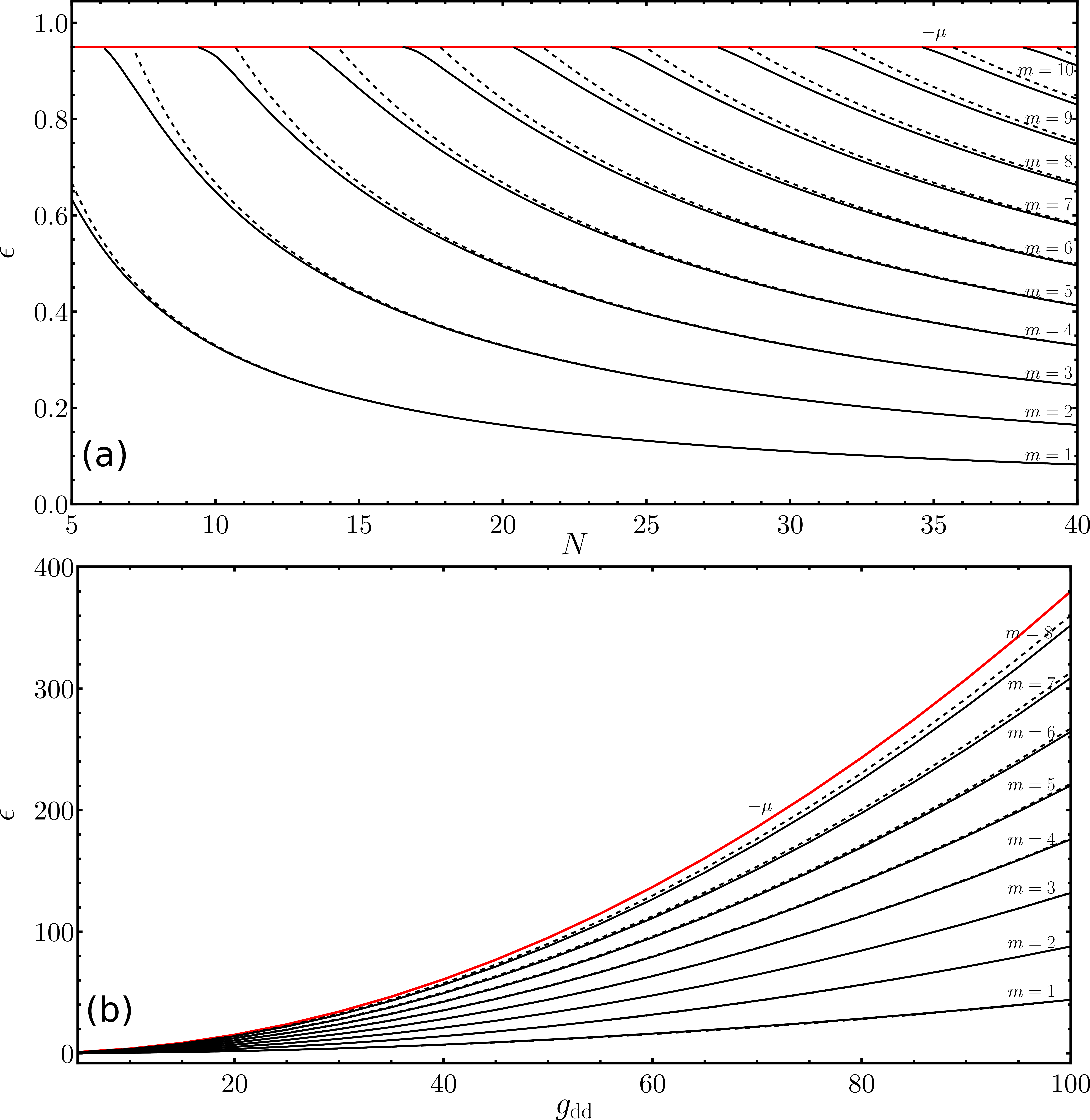
Figure 5: Panel (a): Excitation spectrum of bound modes for a droplet with $g_{\text{dd}}=5$ as a function of particle number $N$. We see that as $N$ grows, the number of bound modes increases and their energies get smaller. Panel (b): Excitation spectrum of bound modes for $N=30$ particles as a function of $g_{\text{dd}}$. The energies are growing functions of $g_{\text{dd}}$. The number of the bound modes does not depend on $g_{\text{dd}}$. In both panels dashed lines mark the results obtained within the framework of rectangular ansatz, Eq. (35).

At this point, it is worth to address two issues. First, analogous excitations were already studied in the droplets in a weakly interacting Bose-Bose mixtures Tylutki et al. (2020), that results from the Gross-Pitaevskii equations extended by the LHY terms Petrov and Astrakharchik (2016b). That results are qualitatively similar to our findings. In both setups, droplets have bound modes displaying phononic dispersion relation and scattering modes. Moreover, the number of bound modes is finite and scales proportionally to $N$ for large droplets. To understand these analogies, one can note that both equations are similar in the sense that they are local equations with competing nonlinearities. In fact, the only difference lies in the different power-law dependence of the terms corresponding to the repulsion and attraction in the system. This analogy in principle may be broken in the regime, where the range of interactions is comparable to the width of the droplet and Eq. (8) becomes truly non-local.

Solving the BdG equations for general case of finite $g$ and $\sigma$ is difficult. On the other hand, we have observed a good agreement between numerical solutions of BdG equations and analytical results based on the simple rectangular ansatz. The latter can be applied for any $g$ and $\sigma$ and practically require only flat-top density profile. Therefore, in the next section we briefly generalize results from this section to parameters outside analytical regime.

III.2 General case in the flat-top regime

The BdG equations (25a) and (25b) used for the case of the rectangular ansatz, but without imposing any restrictions on $g$ and $\sigma$ take the form

$$\epsilon u(x)=\Big{(}-\frac{1}{2}\partial_{x}^{2}+v_{\text{LL}}^{2}[N/L]+\mathcal{J}\Big{)}u(x)+\Big{(}v_{\text{LL}}^{2}[N/L]+\mathcal{J}\Big{)}v(x),$$ (37a)

$$- \epsilon v(x)=\Big{(}-\frac{1}{2}\partial_{x}^{2}+v_{\text{LL}}^{2}[N/L]+\mathcal{J}\Big{)}v(x)+\Big{(}v_{\text{LL}}^{2}[N/L]+\mathcal{J}\Big{)}u(x),$$ (37b)

where we defined the following operator

$$\mathcal{J}h(x)=-\frac{g_{\text{dd}}N}{W}\int dx^{\prime}V_{\text{dd}}^{\sigma}(x-x^{\prime})h(x^{\prime}),$$ (38)

and the Lieb-Liniger speed of sound Lieb and Liniger (1963); Ristivojevic (2014)

$$v_{\text{LL}}[N/W]=\frac{N}{W}\sqrt{3e_{\rm LL}(\gamma_{W})-2\gamma_{W}e_{\rm LL}^{\prime}(\gamma_{W})+\frac{1}{2}\gamma_{W}^{2}e_{\rm LL}^{\prime\prime}(\gamma_{W})}.$$ (39)

Let us remind that the width of the optimal ansatz rectangle $W$ is determined here numerically from the Eq. (19). We find solutions of these equations in the form of standing waves and obtain their spectrum:

$$\epsilon(p)=\sqrt{\Big{(}v_{\text{LL}}^{2}[N/W]-\frac{g_{\text{dd}}N}{W}\hat{V}_{\text{dd}}^{\sigma}(p)\Big{)}p^{2}+\Big{(}\frac{p^{2}}{2}\Big{)}^{2}}.$$ (40)

where $p=\frac{\pi}{W},\frac{2\pi}{W},\ldots$ and $\hat{V}_{\text{dd}}^{\sigma}(p)$ denotes the Fourier transform of the dipolar potential. The number of bound modes can be determined from the transcendental equation $\epsilon(\pi m_{\text{max}}/W)=-\mu=-\mu_{\text{LL}}[N/W]+g_{\text{dd}}N/W$. By taking the limits $g\to\infty$ and $\sigma\to 0$ on the Eq. (40) we obtain, as a special case, the formula (34).

Let us emphasize once again that the results for nonzero $\sigma$ and finite $g$ rely on the assumption, that the stationary density profile is well approximated by a rectangle. In general, this does not have to be the case, as the Eq. (8) has solutions that are closer to Gaussian-like solitonic shapes Ołdziejewski et al. (2020). In such situations, excitation spectrum will differ significantly and one should attempt to solve the full BdG equations.

IV Nonlinear response to a perturbation

In this section we wish to go beyond the linearized version of the dynamics given by Eq. (II). Precisely, to understand better the low energy dynamics of the droplets we numerically solve the full time-dependent equation (II). As initial states we take droplets perturbed with the modes found from BdG equations, analyzed in detail in the previous section. In particular, we want to check the differences between linearized dynamics and the full, nonlinear one given by (II).

The results are presented in Fig. 6. In the first two cases, corresponding to Fig. 6 (a,b), we consider a droplet with the same parameters as in Fig. 4, namely $N=30$, $g_{\text{dd}}=100$ and $\sigma=0$. In Fig. 6(a) we study the dynamics of a bound mode with $m=3$ with the excitation energy given by (35) and the shape proportional to cosine standing wave $u(x),v(x)\sim\cos\frac{3\pi x}{W}$.

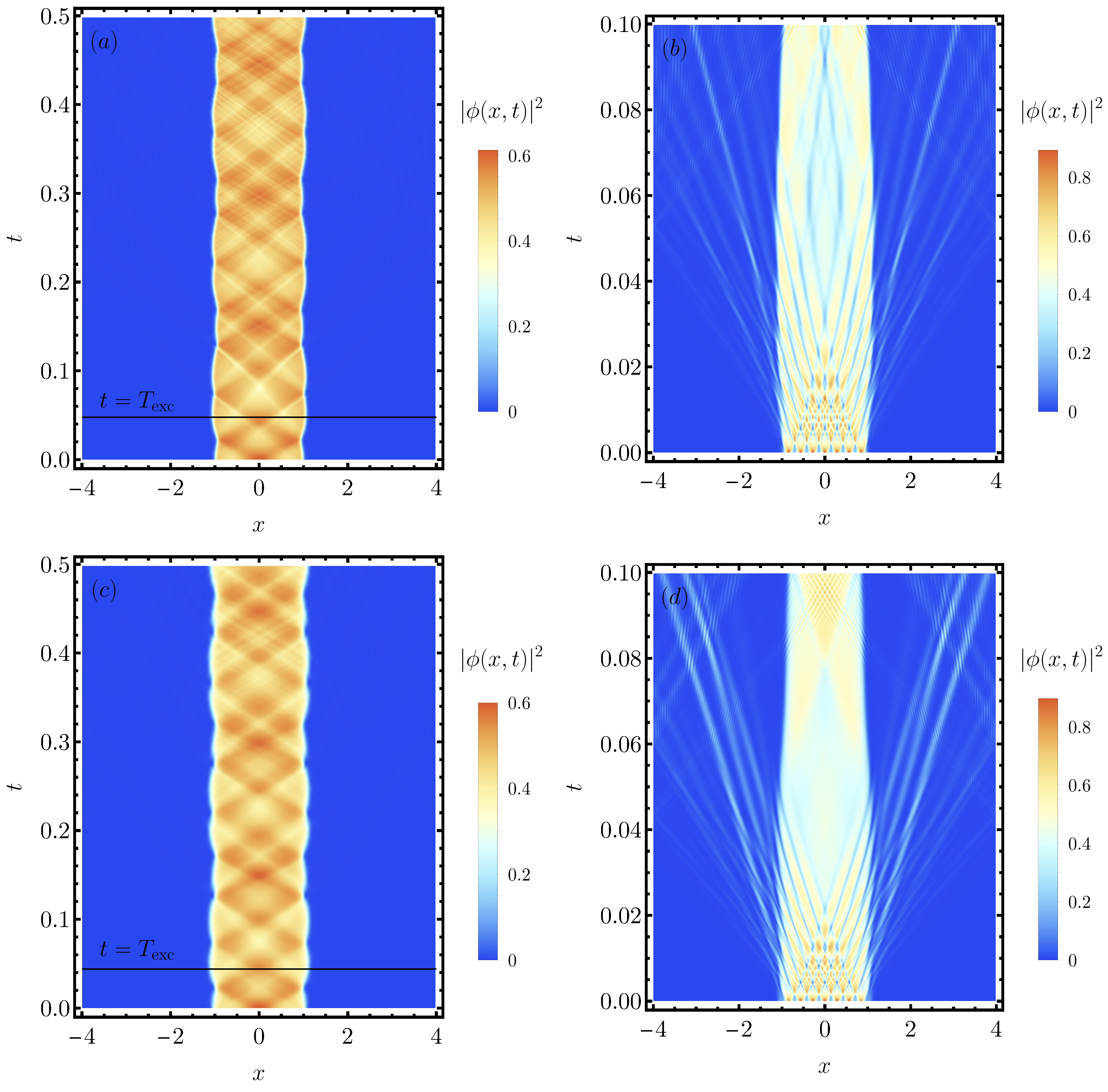
Figure 6: Dynamics of the perturbed droplet with $N=30$, $g_{\text{dd}}=100$ and $\sigma=0$ (first row) or $\sigma=0.05$ (second row). First column: time evolution of bound cosine mode with $m=3$, revival time of the wave matches the period $T_{\text{exc}}$ related to the excitation energy given by (35) for the first row and (40) for the second row. Second column: dynamics of $m=14$ cosine mode, with the excitation energy above the chemical potential. We see the emission of particles in the course of time evolution.

As the excitation energy is below chemical potential, such a perturbation does not lead to the emission of particles from the droplet. After some time, the nonlinear character of evolution brings additional frequencies to the dynamics. Nevertheless, for short times the evolution is governed by a single frequency, given by the excitation energy. This can be seen from the good agreement between revival time of the excited wave and $T_{\text{exc}}=2\pi/\epsilon_{3}$, cf. black line on Fig. 6(a). The situation is drastically different when we consider a mode with an excitation energy higher than the chemical potential. Droplet for our parameters supports eight bound modes, and perturbing it with higher cosine modes should lead to emission of particles. As we see in Fig. 6(b), where the dynamics of $m=14$ cosine mode is presented, this is indeed the case. After short time, particles are emitted and the dynamics in the bulk cannot be described as a single wave that propagates inside and is reflected from the edges.

In Figs.6(c,d) we consider evolution of the same modes, but in the system with nonzero range of dipolar interactions $\sigma=0.05$. We observe that this change makes no qualitative difference in the behavior of the system, suggesting that the general picture of excitations seen in the analytical regime may be valid for flat-top droplets with longer range of dipolar forces. The dynamics presented in this section confirms and supplements the conclusions drawn from the analysis of excitations in the BdG framework.

V Summary and outlook

We have studied flat-top dipolar Tonks-Girardeau droplets, namely quasi 1D droplets in the regime of strong contact interaction. We derived simple approximate formulas for the most important quantities characterizing such a droplet. In between we have found the formulas for the energy of the bulk, and the energy of a droplet edge, i.e. its ”surface”. We presented the excitations spectrum and the shapes of the excitations. Our analysis was based mainly on two approaches.

In the first approach we focused on the analytical regime, where the energy becomes a local operator, and its ground state is analytically known Baizakov et al. (2009). We linearize the equation of motion around the ground state to derive the local BdG equations and find numerically the exact excitation spectrum. Our results can be applied in the limit of large $g$ and when the dipolar interaction coefficient $g_{\rm dd}$, the number of atoms $N$ and the transverse oscillator length $\sigma$ fulfill the conditions $N\gg 3g_{\text{dd}}\sigma/2\pi^{2}\gg 1$.

The second approach was based on a trivial ansatz – approximating droplet density with a rectangular shape and minimizing total energy with respect to its width. Using it, we derived formulas for the excitation spectrum and the number of ”bound modes”, i.e. internal droplet excitations, also beyond the validity regime of the first approach.

We benchmarked the two approaches in the common validity regime, obtaining excellent agreement. We complement this analysis by the simulations of the perturbed droplet dynamics, using the full LLGPE (II). We confirmed the stability of the droplets to perturbation with a bound mode and show that to perturbations with energy above chemical potential induce particle emission from the droplet.

To summarize, the elementary excitations can be characterized as follows. There are two zero-energy modes related to broken symmetries in the system. Next, there is a finite number of bound modes with excitation energies below the chemical potential, whose shapes strongly resemble standing waves of a box with width given by the size of the droplet. These excitations have phononic dispersion relation in the limit of large particle number $N$, moreover the number of these modes is finite and scales proportionally to $N$. In addition to that, a droplet has a continuum spectrum of scattering modes characterized by a non-zero probability of finding a particle outside the droplet.

References

- Petrov (2015) D. Petrov, Phys. Rev. Lett. 115, 155302 (2015).
- Lima and Pelster (2012) A. R. P. Lima and A. Pelster, Phys. Rev. A 86, 063609 (2012).
- Lima and Pelster (2011) A. R. P. Lima and A. Pelster, Phys. Rev. A 84, 041604 (2011).
- Böttcher et al. (2021) F. Böttcher, J.-N. Schmidt, J. Hertkorn, K. S. H. Ng, S. D. Graham, M. Guo, T. Langen, and T. Pfau, Rep. Prog. Phys. 84, 012403 (2021).
- Lee et al. (1957) T. D. Lee, K. Huang, and C. N. Yang, Phys. Rev. 106, 1135 (1957).
- Petrov and Astrakharchik (2016a) D. S. Petrov and G. E. Astrakharchik, Phys. Rev. Lett. 117, 100401 (2016a), arXiv:1605.07585 .
- Edler et al. (2017a) D. Edler, C. Mishra, F. Wächtler, R. Nath, S. Sinha, and L. Santos, Phys. Rev. Lett. 119, 050403 (2017a).
- Astrakharchik and Malomed (2018) G. E. Astrakharchik and B. A. Malomed, Phys. Rev. A 98, 013631 (2018).
- Zin et al. (2018) P. Zin, M. Pylak, T. Wasak, M. Gajda, and Z. Idziaszek, Phys. Rev. A 98, 051603 (2018).
- Ilg et al. (2018) T. Ilg, J. Kumlin, L. Santos, D. S. Petrov, and H. P. Büchler, Phys. Rev. A 98, 051604 (2018).
- Rakshit et al. (2019) D. Rakshit, T. Karpiuk, P. Zin, M. Brewczyk, M. Lewenstein, and M. Gajda, New Journal of Physics 21, 073027 (2019).
- Edmonds et al. (2020) M. Edmonds, T. Bland, and N. Parker, Journal of Physics Communications 4, 125008 (2020).
- Morera et al. (2020) I. Morera, G. E. Astrakharchik, A. Polls, and B. Juliá-Díaz, Phys. Rev. Research 2, 022008 (2020).
- Morera et al. (2021) I. Morera, G. E. Astrakharchik, A. Polls, and B. Juliá-Díaz, Phys. Rev. Lett. 126, 023001 (2021).
- Guijarro et al. (2022) G. Guijarro, G. E. Astrakharchik, and J. Boronat, Phys. Rev. Lett. 128, 063401 (2022).
- Natale et al. (2022) G. Natale, T. Bland, S. Gschwendtner, L. Lafforgue, D. S. Grün, A. Patscheider, M. J. Mark, and F. Ferlaino, arXiv preprint arXiv:2205.03280 (2022).
- Ołdziejewski et al. (2020) R. Ołdziejewski, W. Górecki, K. Pawłowski, and K. Rzazewski, Phys. Rev. Lett. 124, 090401 (2020).
- De Palo et al. (2021) S. De Palo, E. Orignac, M. L. Chiofalo, and R. Citro, Phys. Rev. B 103, 115109 (2021).
- De Palo et al. (2022) S. De Palo, E. Orignac, and R. Citro, Phys. Rev. B 106, 014503 (2022).
- Morera et al. (2022) I. Morera, R. Ołdziejewski, G. E. Astrakharchik, and B. Juliá-Díaz, “Superexchange liquefaction of strongly correlated lattice dipolar bosons,” (2022), arXiv:2204.03906 [cond-mat].
- Kopyciński et al. (2022a) J. Kopyciński, M. Łebek, M. Marciniak, R. Ołdziejewski, W. Górecki, and K. Pawłowski, SciPost Phys. 12, 023 (2022a).
- Edler et al. (2017b) D. Edler, C. Mishra, F. Wächtler, R. Nath, S. Sinha, and L. Santos, Phys. Rev. Lett. 119, 050403 (2017b).
- Tylutki et al. (2020) M. Tylutki, G. E. Astrakharchik, B. A. Malomed, and D. S. Petrov, Phys. Rev. A 101, 051601 (2020).
- Castin and Herzog (2001) Y. Castin and C. Herzog, Comptes Rendus de l’Academie des Sciences de Paris 2 (2001), 10.48550/arXiv.cond-mat/0012040, cond-mat/0012040 .
- Bulgac (2002) A. Bulgac, Phys. Rev. Lett. 89, 050402 (2002).
- Meinert et al. (2015) F. Meinert, M. Panfil, M. J. Mark, K. Lauber, J.-S. Caux, and H.-C. Nägerl, Phys. Rev. Lett. 115, 085301 (2015).
- Kao et al. (2021) W. Kao, K.-Y. Li, K.-Y. Lin, S. Gopalakrishnan, and B. L. Lev, Science 371, 296 (2021).
- Kopyciński et al. (2022b) J. Kopyciński, M. Łebek, W. Górecki, and K. Pawłowski, (2022b), 10.48550/ARXIV.2207.03817.
- Deuretzbacher et al. (2010) F. Deuretzbacher, J. C. Cremon, and S. M. Reimann, Phys. Rev. A 81, 063616 (2010).
- Lieb and Liniger (1963) E. H. Lieb and W. Liniger, Phys. Rev. 130, 1605 (1963).
- Lieb (1963) E. H. Lieb, Phys. Rev. 130, 1616 (1963).
- Lang et al. (2017) G. Lang, F. Hekking, and A. Minguzzi, SciPost Phys. 3, 003 (2017).
- Ristivojevic (2019) Z. Ristivojevic, Phys. Rev. B 100, 081110 (2019).
- Prolhac (2017) S. Prolhac, J. Phys. A: Math. Theor. 50, 144001 (2017).
- Note (1) To keep finite upon decreasing , one should simultaneusly tune to make sufficiently small.
- Baizakov et al. (2009) B. B. Baizakov, F. K. Abdullaev, B. A. Malomed, and M. Salerno, J. Phys. B: At. Mol. Opt. Phys. 42, 175302 (2009).
- Pushkarov et al. (1979) Kh. I. Pushkarov, D. I. Pushkarov, and I. V. Tomov, Opt. Quantum Electron. 11, 471 (1979).
- Kinoshita et al. (2004) T. Kinoshita, T. Wenger, and D. S. Weiss, Science 305, 1125 (2004).
- Paredes et al. (2004) B. Paredes, A. Widera, V. Murg, O. Mandel, S. Fölling, I. Cirac, G. V. Shlyapnikov, T. W. Hänsch, and I. Bloch, Nature 429, 277 (2004).
- Castin (2001) Y. Castin, in Coherent atomic matter waves, Vol. 72, edited by R. Kaiser, C. Westbrook, and F. David (Springer Berlin Heidelberg, Berlin, Heidelberg, 2001) pp. 1–136, series Title: Les Houches - Ecole d’Ete de Physique Theorique.
- Pitaevskii and Stringari (2016) L. Pitaevskii and S. Stringari, Bose-Einstein Condensation and Superfluidity (Oxford University Press, 2016).
- Ronen et al. (2006) S. Ronen, D. C. E. Bortolotti, and J. L. Bohn, Phys. Rev. A 74, 013623 (2006).
- Petrov and Astrakharchik (2016b) D. S. Petrov and G. E. Astrakharchik, Phys. Rev. Lett. 117, 100401 (2016b).
- Ristivojevic (2014) Z. Ristivojevic, Phys. Rev. Lett. 113, 015301 (2014).