Possible origin of HADES data on proton number fluctuations in Au+Au collisions

Abstract

Recent data of the HADES Collaboration in Au+Au central collisions at $\sqrt{s_{\rm NN}}=2.4$ GeV indicate large proton number fluctuations inside one unit of rapidity around midrapidity. This can be a signature of critical phenomena due to the strong attractive interactions between baryons. We study an alternative hypothesis that these large fluctuations are caused by the event-by-event fluctuations of the number of bare protons, and no interactions between these protons are assumed. The proton number fluctuations in five symmetric rapidity intervals $\Delta y$ inside the region $\Delta Y=1$ are calculated using the binomial acceptance procedure. This procedure assumes the independent (uncorrelated) emission of protons, and it appears to be in agreement with the HADES data. To check this simple picture we suggest to calculate the correlation between proton multiplicities in non-overlapping rapidity intervals $\Delta y_{1}$ and $\Delta y_{2}$ placed inside $\Delta Y=1$.

I Introduction

The investigation of the phase diagram of strongly interacting matter is today one of the important topics in nuclear and particle physics. Transitions between different phases are expected to reveal themselves as specific patterns in particle number fluctuations. In particular, a critical point (CP) should yield large fluctuations of the conserved charges Stephanov et al. (1998, 1999); Athanasiou et al. (2010); Stephanov (2009); Kitazawa and Asakawa (2012a); Vovchenko et al. (2016). This generally applies not only to the hypothetical QCD CP which has garnered most attention, but also to the better established CP of the nuclear liquid-gas transition  Sauer et al. (1976); Pochodzalla et al. (1995); Irwin (1937); Vovchenko et al. (2015); Bondorf et al. (1995).

The particle number fluctuations can be characterized by the central moments, $\langle(\Delta N)^{2}\rangle\equiv\sigma^{2}$, $\langle(\Delta N)^{3}\rangle$, $\langle(\Delta N)^{4}\rangle$, etc, where $\langle...\rangle$ denotes the event-by-event averaging and $\Delta N\equiv N-\langle N\rangle$. The scaled variance $\omega$, (normalized) skewness $S\sigma$, and kurtosis $\kappa\sigma^{2}$ of particle number distribution are defined as the following combinations of the central moments,

$$\omega[N] =\frac{\sigma^{2}}{\langle N\rangle}\leavevmode\nobreak\ =\leavevmode\nobreak\ \frac{\kappa_{2}}{\kappa_{1}}\leavevmode\nobreak\ ,$$ (1)

$$S\sigma[N] =\frac{\langle(\Delta N)^{3}\rangle}{\sigma^{2}}\leavevmode\nobreak\ =\leavevmode\nobreak\ \frac{\kappa_{3}}{\kappa_{2}}\leavevmode\nobreak\ ,$$ (2)

$$\kappa\sigma^{2}[N] =\frac{\langle(\Delta N)^{4}\rangle-3\langle(\Delta N)^{2}\rangle^{2}}{\sigma^{2}}\leavevmode\nobreak\ =\leavevmode\nobreak\ \frac{\kappa_{4}}{\kappa_{2}}\leavevmode\nobreak\ ,$$ (3)

where $\kappa_{n}$ are the cumulants of the $N$-distribution. The size-independent (intensive) measures of particle number fluctuations (1-3) are also applied to conserved charges such as net baryon number $B$ and electric charge $Q$.

Having generally longer equilibration times Asakawa et al. (2000); Jeon and Koch (2000), the fluctuations of conserved charges are also thought to reflect properties of earlier stages of collision Kitazawa and Asakawa (2012a). Studies of the higher-order fluctuation measures are motivated by their larger sensitivity to critical phenomena Stephanov (2009, 2011); Schaefer and Wagner (2012); Vovchenko et al. (2015); Chen et al. (2016); Poberezhnyuk et al. (2019). Experimental studies of such fluctuation measures are in progress Luo and Xu (2017).

Total baryon number and electric charge are conserved event-by-event. Therefore, actual fluctuations of conserved charges can only be seen in finite acceptance regions. An optimal choice of acceptance is important problem. If, on the other hand, acceptance is too small, the trivial Poisson-like fluctuations dominate Athanasiou et al. (2010); Poberezhnyuk et al. (2020); Kuznietsov et al. (2022); Pratt and Steinhorst (2020). The acceptance should be large enough compared to correlation lengths relevant for various physics processes  Ling and Stephanov (2016); Vovchenko et al. (2020).

The (net)baryon number fluctuations are expected to be an important signature of any critical phenomena. Because detecting neutrons is problematic, in practice the (net)proton number fluctuations are studied. In central nucleus-nucleus collisions the (net)proton fluctuations are measured at different collision energies as a function of size of a rapidity interval $\Delta y$. At high collision energies fluctuations correspond to the Poisson distribution at small $\Delta y\ll 1$ and they decreases monotonously with $\Delta y$. An explanation of this behavior was recently considered in Refs. Vovchenko and Koch (2021); Savchuk et al. (2022). The main physical effects suppressing the proton number fluctuations are the global baryon number conservation and excluded volume repulsive interactions between protons.

Recently the HADES Collaboration data for proton number fluctuations Adamczewski-Musch et al. (2020) were reported for 5% central Au+Au collisions at the center of mass collision energy of nucleon pairs $\sqrt{s_{\rm NN}}=2.42$ GeV. Note that at this small energy the antiproton production is negligible. In contrast to the data at RHIC and LHC energies the HADES results demonstrate that the scaled variance for protons increases monotonously with $\Delta y$ from unity at $\Delta y\ll 1$ to $\omega>2$ in the symmetric rapidity interval $\Delta Y=1$ in the center of mass system. The effects of baryon conservation and repulsion that appear to drive the behavior of proton number cumulants at high energies fail to describe the HADES data even qualitatively Vovchenko (2022).

Large event-by-event fluctuations of proton number can potentially be a signal of abnormal hadron matter equation of state. This possibility is discussed in Ref. Vovchenko and Koch (2022), which requires strong correlations among the emitted protons in the coordinate space, e.g. due to a possible presence of the critical point in the baryon-rich regime. In the present paper we consider an alternative possibility when no interactions between the detected protons are assumed.

The paper is organized as follows. In Sec. II we present the formulas of the binomial acceptance procedure which connect the fluctuations measures in the finite acceptances with the corresponding quantities in the full phase space. In Sec. III the HADES results are fitted within the the binomial acceptance procedure. Conclusions in Sec. IV closes the article.

II Binomial acceptance procedure

To connect the fluctuations in different rapidity intervals we assume that acceptance of particles is binomial, i.e. that each particle of a given type is accepted by detector with a fixed probability $\alpha$ Bzdak and Koch (2012); Kitazawa and Asakawa (2012b). This probability $0\leq\alpha=\langle n\rangle/\langle N\rangle\leq 1$ equals the ratio of the mean number $\langle n\rangle$ of particles accepted in a fixed region of momentum space $\Delta y$ to the mean number $\langle N\rangle$ of particles of the same type in a “full” momentum space $\Delta Y$. A full momentum space does not necessary means complete $4\pi$-acceptance. The sufficient condition for $\Delta Y$ is to fully encompass $\Delta y$. The main assumption of the binomial acceptance is that the probability $\alpha$ is the same for all particles of a given type and independent of any properties of a specific event. This assumption allows to relate the cumulants within a finite acceptance to their values in the larger, encompassing phase space.

Let the function $P(N)$ be a normalized probability distribution for observing $N$ particles of a given type in the “full” phase space. Assuming the binomial acceptance for particles, the probability $p(n,\alpha)$ to observe $n$ particles detected in the finite $\alpha$-region of the phase space is

$$p(n,\alpha) =\sum_{N=n}^{\infty}\frac{N!}{n!(N-n)!}\,\alpha^{n}(1-\alpha)^{N-n}\,P(N)$$

$$\equiv\sum_{N=n}^{\infty}B(N,n|\alpha)\,P(N)\leavevmode\nobreak\ .$$ (4)

The scaled variance, skewness, and kurtosis of the accepted particles in $\Delta y\leq 1$ are then presented using the distribution (II) as follows Savchuk et al. (2020):

$$\omega_{\alpha}[n] \equiv\frac{\kappa_{2}[n|\alpha]}{\kappa_{1}[n|\alpha]}=1-\alpha+\alpha\omega[N]\leavevmode\nobreak\ ,$$ (5)

$$S\sigma_{\alpha}[n] =\frac{\kappa_{3}[n|\alpha]}{\kappa_{2}[n|\alpha]}=\frac{\omega[N]}{\omega_{\alpha}[n]}\left\{\alpha^{2}S\sigma[N]+3\alpha(1-\alpha)\right\}$$

$$+\frac{1-\alpha}{\omega_{\alpha}[n]}(1-2\alpha)\leavevmode\nobreak\ ,$$ (6)

$$\kappa\sigma^{2}_{\alpha}[n] =\frac{\kappa_{4}[n|\alpha]}{\kappa_{2}[n|\alpha]}=\frac{\displaystyle\omega[N]}{\displaystyle\omega_{\alpha}[n]}\left\{\alpha^{3}\kappa\sigma^{2}[N]\right\}$$ (7)

$$+\frac{\displaystyle\omega[N]}{\displaystyle\omega_{\alpha}[n]}(1-\alpha)\left\{6\alpha^{2}S\sigma[N]+\alpha(7-11\alpha)\right\}$$

$$+\frac{\displaystyle 1-\alpha}{\displaystyle\omega_{\alpha}[n]}\left\{1-6\alpha(1-\alpha)\right\}\leavevmode\nobreak\ ,$$

where $\omega$, $S\sigma$, and $\kappa\sigma^{2}$ correspond to acceptance interval $\Delta Y$ and are given by Eqs. (1-3).

At $\alpha\to 1$ in Eqs. (5-7), one evidently finds $\omega_{\alpha}[n]\to\omega[N]$, $S\sigma_{\alpha}[n]\to S\sigma[N]$, and $\kappa\sigma^{2}_{\alpha}[n]\to\kappa\sigma^{2}[N]$, i.e., the binomial acceptance results approach those in the full rapidity region $\Delta Y=1$. In the opposite limit, $\alpha\to 0$, the cumulant ratios are Poissonian, and $\omega_{\alpha}[n]$, $S\sigma_{\alpha}[n]$, $\kappa\sigma^{2}_{\alpha}[n]\to 1$.

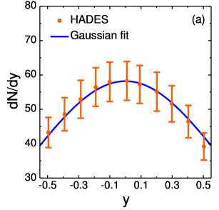
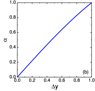
Figure 1: (a): The HADES rapidity distribution are presented by symbols and solid line shows the gaussian fit (8). (b): Acceptance $\alpha$-parameter for the HADES data as a function of the rapidity interval $\Delta y$ calculated using Eq. (9).

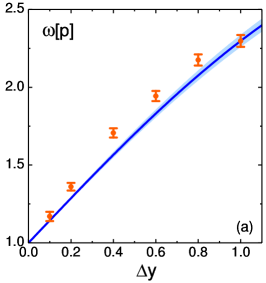
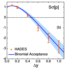
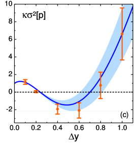
Figure 2: Scaled variance (a), skewness (b), and kurtosis (c) of proton number fluctuations as functions of the rapidity interval $\Delta y$. The HADES data are shown by the symbols. The line corresponds to the binomial acceptance formulas (5-7). The blue bands represent uncertainties due to HADES data errors in the $\Delta Y=1$ rapidity interval.

III HADES results for proton number fluctuations

To describe the proton number fluctuations in Au+Au central collisions at $\sqrt{s_{\rm NN}}=2.42\leavevmode\nobreak\ {\rm GeV}$ as measured by the HADES Collaboration we use the binomial acceptance procedure outlined in Sec. II. The HADES data for $\omega$, $S\sigma$, and $\kappa\sigma^{2}$ are presented for 6 symmetric rapidity intervals $\Delta y=0.1,\leavevmode\nobreak\ 0.2,\leavevmode\nobreak\ 0.4\leavevmode\nobreak\ ,0.6,\leavevmode\nobreak\ 0.8$, and $\Delta Y=1$ in the center of mass system. A transverse momentum cut $0.4<p_{T}<1.6$ GeV/$c$ was applied. In what follows we view the largest rapidity interval $\Delta Y=1$ as a “full” phase space. The quantities $\omega[N]$, $S\sigma[N]$, and $\kappa\sigma^{2}[N]$ for this rapidity interval are then considered as values in the full space (1-3). They are the input parameters for the binomial acceptance formulas (5-7).

The first step of the binomial acceptance procedure is calculating the corresponding $\alpha$-probabilities for different rapidity intervals. In Fig. 1 (a) the preliminary HADES data of the proton rapidity distribution for 10% most central Au+Au collisions Szala (2020); Harabasz et al. (2020) are presented in the rapidity interval $\Delta Y=1$. We fit these data by the gaussian distribution

$$\frac{dN}{dy}\leavevmode\nobreak\ =\leavevmode\nobreak\ C\leavevmode\nobreak\ \exp\left[\leavevmode\nobreak\ -\frac{y^{2}}{2a^{2}}\right]\leavevmode\nobreak\ ,$$ (8)

with two parameters $C=90/\sqrt{2\pi a^{2}}$ and $a=0.62$ which estimate the height and the width of the distribution. For any $\Delta y\leq 1$ one defines the $\alpha$-probabilities as

$$\alpha\leavevmode\nobreak\ =\leavevmode\nobreak\ \frac{\int\limits_{-\Delta y/2}^{\Delta y/2}\,dy\leavevmode\nobreak\ dN/dy}{\int\limits_{-1/2}^{1/2}\,dy\leavevmode\nobreak\ dN/dy}\leavevmode\nobreak\ .$$ (9)

The acceptance parameter $\alpha$ as a function of $\Delta y$ is shown in Fig. 1 (b).

The scaled variance $\omega_{\alpha}[n]$, skewness $S\sigma_{\alpha}[n]$, and kurtosis $\kappa\sigma^{2}_{\alpha}[n]$ of proton number fluctuations as functions of $\Delta y$ are shown in Fig. 2. One can see that the binomial acceptance procedure gives a good agreement with the HADES data for all $\Delta y<1$. Thus, knowledge of “global” cumulants (in the rapidity interval $\Delta Y=1$) is sufficient to restore the corresponding values for any $\Delta y<1$, and no “local” correlations between protons within $\Delta Y$ are observed.

To find the signatures of these global fluctuations we suggest calculating the correlation function for two arbitrary non-overlapping rapidity regions $\Delta y_{1}$ and $\Delta y_{2}$, both inside the symmetric interval $\Delta Y=1$, with $\langle N\rangle$ being the average number of protons inside the interval $\Delta Y=1$ (see Appendix):

$$\rho(n_{1},n_{2})\equiv\leavevmode\nobreak\ \langle N\rangle\frac{\langle n_{1}n_{2}\rangle-\langle n_{1}\rangle\langle n_{2}\rangle}{\langle n_{1}\rangle\langle n_{2}\rangle}=\omega[N]-1\leavevmode\nobreak\ .$$ (10)

Equation (10) demonstrates the universal positive, as $\omega[N]>1$, correlations between $n_{1}$ and $n_{2}$. These correlations are independent of both the sizes of $\Delta y_{1}$ and $\Delta y_{2}$ and of their locations inside the rapidity interval $\Delta Y=1$. Note that for $\omega[N]=0$ these correlations would be negative and equal $\rho=-1$ as a consequence of the global $N$-conservation in the $\Delta Y=1$ interval. The negative values $-1\leq\rho\leq 0$ correspond to small $N$-fluctuations with $0\leq\omega[N]\leq 1$. It would be interesting to check the relation (10) from the HADES data.

IV Conclusions

The binomial acceptance procedure describes the scaled variance, skewness, and kurtosis of proton number fluctuations measured recently by HADES Collaboration in 5% central Au+Au collisions at $\sqrt{s_{\rm NN}}=2.42$ GeV in multiple rapidity intervals. Binomial acceptance formulas connect the observed large proton number fluctuations in the rapidity interval $\Delta Y=1$ with the observed proton number fluctuations. This is consistent with the absence of local correlations between proton momenta inside the rapidity interval $\Delta Y=1$.

The existing HADES data show large non-gaussian fluctuations of the number of protons within the rapidity interval $\Delta Y=1$. These large fluctuations can be due to anomalies in the equation of state of matter created in the collision which manifest themselves as local interproton correlations in the coordinate space. However, large fluctuations can also emerge due to some global external reasons which are valid even for a system of non-interacting particles.

An evident reason for the global proton number fluctuations could be event-by-event fluctuations in the number of nucleon participants. One should exclude this trivial source of event-by-event fluctuations. At small collision energies this is not an easy problem: there is no clear criterion to distinguish between the spectator and participant nucleons. The HADES data are corrected for volume fluctuations Adamczewski-Musch et al. (2020). However, additional studies in this direction would be helpful.

Another complication at the collision energy this low is the significant presence of light nuclear fragments in the final state. The existence of a large fraction of baryons in the form of nuclear fragments can generate large fluctuations of the number of bare protons. Finally, collective flows of baryons at low collision energies appear to be rather small which causes a problem to transfer the particle correlations from coordinate to momentum space.

An interesting consequence of the picture with the global proton number fluctuations and no local correlations between proton momenta is a universal form (10) for the correlations of multiplicities in two arbitrary non-overlapping rapidity intervals $\Delta y_{1}$ and $\Delta y_{2}$, both inside the rapidity region $\Delta Y=1$. The relation (10) can be checked using the existing HADES data for protons at $\sqrt{s_{\rm NN}}=2.42\leavevmode\nobreak\ {\rm GeV}$.

Appendix A Derivation of Eq. (10)

Let $\Delta y_{1}$ and $\Delta y_{2}$ be the non-overlapping rapidity regions, both inside the interval $[-0.5,0.5]$, containing $n_{1}$ and $n_{2}$ particles, respectively. The number of particles $N$ in the interval $[-0.5,0.5]$ is described by the probability distribution $P(N)$. For uncorrelated particles the particle number distribution $P(n_{1},n_{2};N)$ can be presented in the following form:

$$P(n_{1},n_{2};N)=P(N)B(N,n_{2}|\alpha_{2})B(N-n_{2},n_{1}|\alpha_{1})\leavevmode\nobreak\ ,$$ (11)

where $\alpha_{1}=\langle n_{1}\rangle/(\langle N\rangle-\langle n_{2}\rangle)$ and $\alpha_{2}=\langle n_{2}\rangle/\langle N\rangle$. Using Eq. 11 one then finds

$$\langle n_{1}n_{2}\rangle =\sum_{N}\sum_{n_{1},n_{2}}n_{1}n_{2}\leavevmode\nobreak\ P(n_{1},n_{2};N)\leavevmode\nobreak\$$

$$=\leavevmode\nobreak\ \langle n_{1}\rangle\langle n_{2}\rangle\left(1+\frac{\omega[N]-1}{N}\right)\leavevmode\nobreak\ .$$ (12)

References

- Stephanov et al. (1998) M. A. Stephanov, K. Rajagopal, and E. V. Shuryak, Phys. Rev. Lett. 81, 4816 (1998), arXiv:hep-ph/9806219 [hep-ph] .
- Stephanov et al. (1999) M. A. Stephanov, K. Rajagopal, and E. V. Shuryak, Phys. Rev. D60, 114028 (1999), arXiv:hep-ph/9903292 [hep-ph] .
- Athanasiou et al. (2010) C. Athanasiou, K. Rajagopal, and M. Stephanov, Phys. Rev. D82, 074008 (2010), arXiv:1006.4636 [hep-ph] .
- Stephanov (2009) M. A. Stephanov, Phys. Rev. Lett. 102, 032301 (2009), arXiv:0809.3450 [hep-ph] .
- Kitazawa and Asakawa (2012a) M. Kitazawa and M. Asakawa, Phys. Rev. C 86, 024904 (2012a).
- Vovchenko et al. (2016) V. Vovchenko, R. V. Poberezhnyuk, D. V. Anchishkin, and M. I. Gorenstein, J. Phys. A49, 015003 (2016), arXiv:1507.06537 [nucl-th] .
- Sauer et al. (1976) G. Sauer, H. Chandra, and U. Mosel, Nucl. Phys. A264, 221 (1976).
- Pochodzalla et al. (1995) J. Pochodzalla et al., Phys. Rev. Lett. 75, 1040 (1995).
- Irwin (1937) J. O. Irwin, Journal of the Royal Statistical Society 100, 415 (1937).
- Vovchenko et al. (2015) V. Vovchenko, D. V. Anchishkin, M. I. Gorenstein, and R. V. Poberezhnyuk, Phys. Rev. C92, 054901 (2015), arXiv:1506.05763 [nucl-th] .
- Bondorf et al. (1995) J. P. Bondorf, A. S. Botvina, A. S. Ilinov, I. N. Mishustin, and K. Sneppen, Phys. Rept. 257, 133 (1995).
- Asakawa et al. (2000) M. Asakawa, U. W. Heinz, and B. Muller, Phys. Rev. Lett. 85, 2072 (2000), arXiv:hep-ph/0003169 [hep-ph] .
- Jeon and Koch (2000) S. Jeon and V. Koch, Phys. Rev. Lett. 85, 2076 (2000), arXiv:hep-ph/0003168 [hep-ph] .
- Stephanov (2011) M. A. Stephanov, Phys. Rev. Lett. 107, 052301 (2011), arXiv:1104.1627 [hep-ph] .
- Schaefer and Wagner (2012) B. J. Schaefer and M. Wagner, Phys. Rev. D85, 034027 (2012), arXiv:1111.6871 [hep-ph] .
- Chen et al. (2016) J.-W. Chen, J. Deng, H. Kohyama, and L. Labun, Phys. Rev. D93, 034037 (2016), arXiv:1509.04968 [hep-ph] .
- Poberezhnyuk et al. (2019) R. Poberezhnyuk, V. Vovchenko, A. Motornenko, M. I. Gorenstein, and H. Stoecker, (2019), arXiv:1906.01954 [hep-ph] .
- Luo and Xu (2017) X. Luo and N. Xu, Nucl. Sci. Tech. 28, 112 (2017), arXiv:1701.02105 [nucl-ex] .
- Poberezhnyuk et al. (2020) R. V. Poberezhnyuk, O. Savchuk, M. I. Gorenstein, V. Vovchenko, K. Taradiy, V. V. Begun, L. Satarov, J. Steinheimer, and H. Stoecker, Phys. Rev. C 102, 024908 (2020).
- Kuznietsov et al. (2022) V. A. Kuznietsov, O. Savchuk, M. I. Gorenstein, V. Koch, and V. Vovchenko, Phys. Rev. C 105, 044903 (2022).
- Pratt and Steinhorst (2020) S. Pratt and R. Steinhorst, Phys. Rev. C 102, 064906 (2020).
- Ling and Stephanov (2016) B. Ling and M. A. Stephanov, Phys. Rev. C93, 034915 (2016), arXiv:1512.09125 [nucl-th] .
- Vovchenko et al. (2020) V. Vovchenko, O. Savchuk, R. V. Poberezhnyuk, M. I. Gorenstein, and V. Koch, Physics Letters B 811, 135868 (2020).
- Vovchenko and Koch (2021) V. Vovchenko and V. Koch, Phys. Rev. C 103, 044903 (2021).
- Savchuk et al. (2022) O. Savchuk, V. Vovchenko, V. Koch, J. Steinheimer, and H. Stoecker, Physics Letters B 827, 136983 (2022).
- Adamczewski-Musch et al. (2020) J. Adamczewski-Musch et al. (HADES), Phys. Rev. C 102, 024914 (2020), arXiv:2002.08701 [nucl-ex] .
- Vovchenko (2022) V. Vovchenko, (2022), arXiv:2208.13693 [hep-ph] .
- Vovchenko and Koch (2022) V. Vovchenko and V. Koch, Phys. Lett. B 833, 137368 (2022), arXiv:2204.00137 [hep-ph] .
- Bzdak and Koch (2012) A. Bzdak and V. Koch, Phys. Rev. C 86, 044904 (2012).
- Kitazawa and Asakawa (2012b) M. Kitazawa and M. Asakawa, Phys. Rev. C 85, 021901 (2012b).
- Savchuk et al. (2020) O. Savchuk, R. V. Poberezhnyuk, V. Vovchenko, and M. I. Gorenstein, Phys. Rev. C 101, 024917 (2020).
- Szala (2020) M. Szala (HADES), Springer Proc. Phys. 250, 297 (2020).
- Harabasz et al. (2020) S. Harabasz, W. Florkowski, T. Galatyuk, M. Gumberidze, R. Ryblewski, P. Salabura, and J. Stroth, Phys. Rev. C 102, 054903 (2020).