A new T-compatibility condition and its application to the discretization of the damped time-harmonic Galbrun’s equation

Abstract

We consider the approximation of weakly T-coercive operators. The main property to ensure the convergence thereof is the regularity of the approximation (in the vocabulary of discrete approximation schemes). In a previous work the existence of discrete operators $T_{n}$ which converge to $T$ in a discrete norm was shown to be sufficient to obtain regularity. Although this framework proved useful for many applications for some instances the former assumption is too strong. Thus in the present article we report a weaker criterium for which the discrete operators $T_{n}$ only have to converge point-wise, but in addition a weak T-coercivity condition has to be satisfied on the discrete level. We apply the new framework to prove the convergence of certain $H^{1}$-conforming finite element discretizations of the damped time-harmonic Galbrun’s equation, which is used to model the oscillations of stars. A main ingredient in the latter analysis is the uniformly stable invertibility of the divergence operator on certain spaces, which is related to the topic of stable discretizations of the Stokes equation.

Keywords: discrete approximation schemes, weak T-coercivity, Galbrun’s equation
MSC Classification: 35L05, 35Q85, 65N30

1 Introduction

An origin of the T-coercivity technique to analyze equations of non weakly coercive form can be found in the theory of Maxwell’s equation and goes back at least to [11, 10]. The idea to use a discrete variant to prove the stability of approximations can be found e.g. in [29, 7]. In [21] this approach was formalized to a framework to prove the convergence of Galerkin approximations of holomorphic eigenvalue problems and was successfully applied for perfectly matched layer methods to scalar isotropic [19] and anisotropic [23] materials, Maxwell problems in conductive media [21], modified Maxwell Steklov problems [20] and Maxwell transmission problems for dispersive media [40, 25]. In particular [21] is build upon the much broader framework of discrete approximation schemes [39, 41] which originated in the 1970s and the best results for eigenvalue problems in this context are [32, 33]. The main contribution of [21] was to provide a practical criterium to prove the regularity of approximations, which allows to apply the results achieved for discrete approximation schemes. Although for some applications it turns out that the T-compatibility criterion of [21] is too strong, and hence we present in this article a weaker variant. Some similarity can be drawn to the analysis of p-finite element methods for Maxwell problems [6], for which (opposed to h-finite element methods) the cochain projections are not uniformly $L^{2}$ bounded, and hence the discrete compactness property is obtained in [6] by an alternative technique.

The present article is motivated by the study of approximations to the damped time-harmonic Galbrun equation. The Galbrun equation [15] is a linearization of the nonlinear Euler equations with the Lagrangian perturbation of displacement as unknown, and is used in aeroacoustics [35] as well as in an extended version in asteroseismology [34]. We refer to [18] for a well-posedness analysis in the time domain. In the time-harmonic domain an approach in aeroacoustics is to use a stabilized formulation, which is justified by the introduction of an additional transport equation for the vorticity, and we refer to the well-posedness analysis in [8]. Different to aeroacoustics in asteroseismology there exists a significant damping of waves which allows the equation to be analyzed in a more direct way, see the well-posedness results [26, 22]. In the second part of the present article we apply our new framework to the approximation of the damped time-harmonic Galbrun’s equation as considered in [26]:

$$\begin{aligned} -\rho(\omega+i\partial_{\mathbf{b}}+i\Omega\times)^{2}\mathbf{u}&-\nabla\left(\rho c_{s}^{2}\operatorname{div}\mathbf{u}\right)+(\operatorname{div}\mathbf{u})\nabla p\\ &-\nabla(\nabla p\cdot\mathbf{u})+(\operatorname{Hess}(p)-\rho\operatorname{Hess}(\phi))\mathbf{u}+\gamma\rho(-i\omega)\mathbf{u}=\mathbf{f}\quad\mbox{in }\mathcal{O}\end{aligned}$$ (1)

where $\rho,p,\phi,c_{s},\mathbf{b},\Omega$ and $\mathbf{f}$ denote density, pressure, gravitational potential, sound speed, background velocity, angular velocity of the frame and sources, $\partial_{\mathbf{b}}:=\sum_{l=1}^{3}\mathbf{b}_{l}\partial_{x_{l}}$ denotes the directional derivative in direction $\mathbf{b}$, $\operatorname{Hess}(p)$ the Hessian of $p$, $\mathcal{O}\subset\mathbb{R}^{3}$ a bounded domain, and damping is modeled by the term $-i\omega\gamma\rho\mathbf{u}$ with damping coefficient $\gamma$. The main challenge to tackle this equation can already be observed in the case $p,\phi=0,\Omega=0$. We discretize (1) with conforming $\mathbf{H}^{1}$ finite elements. To guarantee the stability of the approximation we use vectorial finite element spaces which admit a suitable uniformly stable inversion of the divergence operator. In particular, let $X_{h}\subset\mathbf{H}^{1}$ be a Lagrangian vectorial finite element space of order $k$ and $Q_{h}\subset L^{2}$ be a scalar finite element space and $L^{2}_{0}:=\{u\in L^{2}\colon\int_{\Omega}u\,\mathrm{d}x=0\}$. Then we require that there exists a uniformly bounded inverse of the (discrete) divergence operator acting on the spaces $Q_{h}\cap L^{2}_{0}\to X_{h}\cap\mathbf{H}^{1}_{0}$. Such methods have been developed in the field of computational fluid dynamics for the stable discretization of incompressible Stokes and Navier-Stokes equations, cf. e.g. [30].

Especially convenient for the analysis are the so-called divergence free finite elements, meaning that the approximative solutions to the Stokes equations are exactly divergence free. However, note that there exist sophisticated techniques to construct such elements and not all divergence free finite elements fit our needs. The pioneering work for divergence free finite elements was set by Scott and Vogelius [38], who established respective results (suitable for our purpose) in 2D for triangular quasi-uniform meshes with finite degree of degenerecy and polynomial degree $k\geq 4$ (the quasi-uniformity is actually not necessary due to [14]). In three dimensions Zhang [44] reported a generalization to uniform tetrahedral grids for $k\geq 6$, and his results in [43] indicate that for general tetrahedral grids suitable orders are $k\geq 8$. The application of convenient finite element spaces on specialized meshes generated by barycentric refinements (suitable for our purpose) received extensive attention and we refer e.g. to [3, 42, 17]. In general such schemes are related to respective discretizations of suitable deRahm complexes with high regularity [13, 36, 16]. There exist also several results for elements on quadrilateral grids for which we refer to the bibliographies of [31, 36]. Other approaches to construct divergence free finite elements include enriched finite elements, nonconforming elements, discontinuous Galerkin methods and isogeometric methods.

Although we will make use of the advantages of divergence free finite elements in the analysis, we note that the more important property is the stable Stokes approximation. A comparison and analysis of different robust finite element discretizations for a simplified Galbrun’s equation is presented in [2]. An approximation with $H(\operatorname{div})$-conforming finite elements is analyzed in [24].

The remainder of this article is structured as follows. In Section 2 we report a multipurpose framework based on a weak T-compatibility condition (weaker than in [21]) to obtain the regularity and hence the stability of approximations. Although in the present article we consider only conforming discretizations to (1), we formulate the framework in a general way to include also nonconforming approximations. In Section 3 we apply the former framework to discretizations of (1). In particular, in Section 3.5 we consider a simplified case of (1) to present the main ideas and in Section 3.6 we treat the general case. In Section 4 we present computational examples to accompany our theoretical results and we conclude in Section 5.

2 Abstract framework

This section discusses a multipurpose framework for the analysis of approximations of linear operators. In Section 2.1 we review the framework and important definitions, as well as sufficient conditions for the convergence of the approximative solution. We aim to apply this framework to operators that are Fredholm with index zero, however have the structure of ‘coercive+compact’ only up to a bijection. Such operators are called weakly $T$-coercive, a precise definition is given in Section 2.2. Note that this property is equivalent to an operator being Fredholm with index zero, and the construction of a suitable $T$ operator is the tool to prove this property. Here we study a way how this property can be mimiced on the discrete level to ensure convergent approximations.

2.1 Discrete approximation schemes

We consider discrete approximation schemes in Hilbert spaces. Note that the forthcoming setting is a bit more restrictive than the schemes considered in [39, 41, 32], but more convenient for our purposes. For two Hilbert spaces $(X,\langle\cdot,\cdot\rangle_{X})$, $(Y,\langle\cdot,\cdot\rangle_{Y})$ let $L(X,Y)$ be the space of bounded linear operators from $X$ to $Y$, and set $L(X):=L(X,X)$.

We consider a discrete approximation scheme of $A\in L(X)$ in the following way. Let $(X_{n},\langle\cdot,\cdot\rangle_{X_{n}})_{n\in\mathbb{N}}$ be a sequence of finite dimensional Hilbert spaces and $A_{n}\in L(X_{n})$. Note that we do not demand that the spaces $X_{n}$ are subspaces of $X$. Instead we demand that there exist operators $p_{n}\in L(X,X_{n})$ such that $\lim_{n\to\infty}\|p_{n}u\|_{X_{n}}=\|u\|_{X}$ for each $u\in X$. We then define the following properties of a discrete approximation scheme:

• A sequence $(u_{n})_{n\in\mathbb{N}},u_{n}\in X_{n}$ is said to converge to $u\in X$, if $\lim_{n\to\infty}\|p_{n}u-u_{n}\|_{X_{n}}=0$.

• A sequence $(u_{n})_{n\in\mathbb{N}},u_{n}\in X_{n}$ is said to be compact, if for every subsequence $\mathbb{N}^{\prime}\subset\mathbb{N}$ exists a subsubsequence $\mathbb{N}^{\prime\prime}\subset\mathbb{N}^{\prime}$ such that $(u_{n})_{n\in\mathbb{N}^{\prime\prime}}$ converges (to a $u\in X$).

• A sequence $(A_{n})_{n\in\mathbb{N}},A_{n}\in L(X_{n})$ is said to approximate $A\in L(X)$, if $\lim_{n\to\infty}\|A_{n}p_{n}u-p_{n}Au\|_{X_{n}}=0$. In a finite element vocabulary it might be more convenient to denote this property as asymptotic consistency.

• A sequence of operators $(A_{n})_{n\in\mathbb{N}},A_{n}\in L(X_{n})$ is said to be compact, if for every bounded sequence $(u_{n})_{n\in\mathbb{N}},u_{n}\in X_{n}$, $\|u_{n}\|_{X_{n}}\leq C$ the sequence $(A_{n}u_{n})_{n\in\mathbb{N}}$ is compact.

• A sequence of operators $(A_{n})_{n\in\mathbb{N}},A_{n}\in L(X_{n})$ is said to be stable, if there exist constants $C,n_{0}>0$ such that $A_{n}$ is invertible and $\|A_{n}^{-1}\|_{L(X_{n})}\leq C$ for all $n>n_{0}$.

• A sequence of operators $(A_{n})_{n\in\mathbb{N}},A_{n}\in L(X_{n})$ is said to be regular, if $\|u_{n}\|_{X_{n}}\leq C$ and the compactness of $(A_{n}u_{n})_{n\in\mathbb{N}}$ implies the compactness of $(u_{n})_{n\in\mathbb{N}}$.

The central properties we are looking for in a discrete approximation scheme are regularity and asymptotic consistency  which are sufficient for the convergence of discrete solutions. To emphasize this we recall in the following some well known results.

Lemma 1.

Let $A\in L(X)$ be bijective and $(A_{n})_{n\in\mathbb{N}}$, $A_{n}\in L(X_{n})$ be a discrete approximation scheme which is regular and approximates $A$. Then $(A_{n})_{n\in\mathbb{N}}$ is stable.

Proof.

Follows from statement 3) of [32, Theorem 2]. ∎

Lemma 2.

Let $A\in L(X)$ be bijective and $(A_{n})_{n\in\mathbb{N}}$, $A_{n}\in L(X_{n})$ be a discrete approximation scheme which is stable  and approximates $A$. Let $u,u_{n}$ be the solutions to $Au=f$ and $A_{n}u_{n}=f_{n}\in X_{n}$, and $\lim_{n\to\infty}\|p_{n}f-f_{n}\|_{X_{n}}=0$. Then $\lim_{n\to\infty}\|p_{n}u-u_{n}\|_{X_{n}}=0$. If the approximation is a conforming Galerkin scheme, i.e. $X_{n}\subset X$ and $p_{n}$ is the orthogonal projection onto $X_{n}$, $f_{n}=p_{n}f$, then there exist constants $C,n_{0}>0$ such that $\|u-u_{n}\|_{X}\leq C\inf_{u_{n}^{\prime}\in X_{n}}\|u-u_{n}^{\prime}\|_{X}$ for all $n>n_{0}$.

Proof.

Let $n_{0}>0$ be such that $A_{n}$ is invertible for all $n>n_{0}$. We estimate

$$\|p_{n}u-u_{n}\|_{X_{n}} \leq\sup_{m>n_{0}}\|A_{m}^{-1}\|_{L(X_{m})}\|A_{n}p_{n}u-A_{n}u_{n}\|_{X_{n}}$$

$$\leq\sup_{m>n_{0}}\|A_{m}^{-1}\|_{L(X_{m})}\big{(}\|A_{n}p_{n}u-p_{n}Au\|_{X_{n}}+\|p_{n}Au-A_{n}u_{n}\|_{X_{n}}\big{)}$$

$$=\sup_{m>n_{0}}\|A_{m}^{-1}\|_{L(X_{m})}\big{(}\|A_{n}p_{n}u-p_{n}Au\|_{X_{n}}+\|p_{n}f-f_{n}\|_{X_{n}}\big{)}.$$

It holds that $\lim_{n\to\infty}\|A_{n}p_{n}u-p_{n}Au\|_{X_{n}}=0$, because $(A_{n})_{n\in\mathbb{N}}$ approximates $A$; and that $\lim_{n\to\infty}\|p_{n}f-f_{n}\|_{X_{n}}=0$ by assumption. Hence the first claim is proven. For the second claim we estimate

$$\|u-u_{n}\|_{X}\leq\|u-p_{n}u\|_{X}+\|p_{n}u-u_{n}\|_{X} \leq\|u-p_{n}u\|_{X}+\sup_{m>n_{0}}\|A_{m}^{-1}\|_{L(X_{m})}\|p_{n}Ap_{n}u-p_{n}Au\|_{X}$$

$$\leq\|u-p_{n}u\|_{X}+\sup_{m>n_{0}}\|A_{m}^{-1}\|_{L(X_{m})}\|A\|_{L(X)}\|u-p_{n}u\|_{X}$$

$$=\big{(}1+\sup_{m>n_{0}}\|A_{m}^{-1}\|_{L(X_{m})}\|A\|_{L(X)}\big{)}\|u-p_{n}u\|_{X}.$$

∎

2.2 The new T-compatibility condition

An operator $A\in L(X)$ is called coercive, if there exists a constant $C>0$ such that $|\langle Au,u\rangle_{X}|\geq C\|u\|_{X}^{2}$ for all $u\in X$. An operator $A\in L(X)$ is called weakly coercive, if there exists a compact operator $K\in L(X)$ such that $A+K$ is coercive. An operator $A$ is called (weakly) right $T$-coercive, if $T\in L(X)$ is bijective and $AT$ is (weakly) coercive.

The next theorem provides a sufficient setting for a discrete approximation of a (weakly) right $T$-coercive operator. This theorem is key for the discretization and its analysis in Section 3.

Theorem 3.

Assume a constant $C>0$, sequences $(A_{n})_{n\in\mathbb{N}},(T_{n})_{n\in\mathbb{N}},(B_{n})_{n\in\mathbb{N}},(K_{n})_{n\in\mathbb{N}}$ and $B,T\in L(X)$ which satisfy the following: for each $n\in\mathbb{N}$ it holds $A_{n},T_{n},B_{n},K_{n}\in L(X_{n})$, $\|T_{n}\|_{L(X_{n})},\|T_{n}^{-1}\|_{L(X_{n})},\|B_{n}\|_{L(X_{n})},\|B_{n}^{-1}\|_{L(X_{n})}\leq C$, $B$ is bijective, $(K_{n})_{n\in\mathbb{N}}$ is compact and

$$\lim_{n\to\infty}\|T_{n}p_{n}u-p_{n}Tu\|_{X_{n}}=0,\qquad \lim_{n\to\infty}\|B_{n}p_{n}u-p_{n}Bu\|_{X_{n}}=0\qquad\forall u\in X,$$ (2a)

$$A_{n}T_{n}= B_{n}+K_{n}.$$ (2b)

Then $(A_{n})_{n\in\mathbb{N}}$ is regular.

Proof.

Let $(u_{n})_{n\in\mathbb{N}}$, $u_{n}\in X_{n}$ be a uniformly bounded sequence $\|u_{n}\|_{X_{n}}\leq C$, $(f_{n})_{n\in\mathbb{N}}$ with $f_{n}:=A_{n}u_{n}$ be compact, and $\mathbb{N}^{\prime}\subset\mathbb{N}$ be an arbitrary subsequence. Consider a converging subsequence $(f_{n})_{n\in\mathbb{N}^{\prime\prime}}$ with $\mathbb{N}^{\prime\prime}\subset\mathbb{N}^{\prime}$ and denote the limit as $f\in X$ such that $\lim_{n\in\mathbb{N}^{\prime\prime}}\|A_{n}u_{n}-p_{n}f\|_{X_{n}}=0$. We then obtain from (2b) that $B_{n}T_{n}^{-1}u_{n}+K_{n}T_{n}^{-1}u_{n}=A_{n}u_{n}=f_{n}\to f$ for $n\in\mathbb{N}^{\prime\prime},n\to\infty$. Since $T_{n}^{-1}$ is bounded and $(K_{n})_{n\in\mathbb{N}}$ is compact , $(T_{n}^{-1}u_{n})_{n\in\mathbb{N}^{\prime\prime}}$ is bounded and we can choose a converging subsequence $(g_{n})_{n\in\mathbb{N}^{\prime\prime\prime}}$ with $g_{n}=K_{n}T_{n}^{-1}u_{n}$, $\mathbb{N}^{\prime\prime\prime}\subset\mathbb{N}^{\prime\prime}$ and limit $g\in X$ such that $\lim_{n\in\mathbb{N}^{\prime\prime\prime}}\|g_{n}-p_{n}g\|_{X_{h}}=0$. We observe that there holds $u_{n}=T_{n}B_{n}^{-1}(f_{n}-g_{n})$. Finally, we want to exploit the properties in (2a) on $T_{n}$ and $B_{n}$ to show $\lim_{n\in\mathbb{N}^{\prime\prime\prime}}\|u_{n}-p_{n}TB^{-1}(f-g)\|_{X_{h}}=0$ which implies the compactness of $(u_{n})_{n\in\mathbb{N}}$. We start with a triangle inequality

$$\|u_{n}-p_{n}TB^{-1}(f-g)\|_{X_{n}} \leq\underbrace{\|u_{n}-T_{n}B_{n}^{-1}p_{n}(f-g)\|_{X_{n}}}_{I}+\underbrace{\|p_{n}TB^{-1}(f-g)-T_{n}B_{n}^{-1}p_{n}(f-g)\|_{X_{n}}}_{II}$$

and bound the two contributions I and II one after another:

$$I \leq\|T_{n}\|_{L(X_{n})}\|B_{n}^{-1}\|_{L(X_{n})}\|B_{n}T_{n}^{-1}u_{n}-p_{n}(f-g)\|_{X_{n}}=C^{2}\|(f_{n}-g_{n})-p_{n}(f-g)\|_{X_{n}}$$

$$=C^{2}\|(f_{n}-p_{n}f)+(g_{n}-p_{n}g))\|_{X_{n}}\leq C^{2}\big{(}\|f_{n}-p_{n}f\|_{X_{n}}+\|p_{n}-p_{n}g\|_{X_{n}}\big{)},$$

$$II \leq\|p_{n}TB^{-1}(f-g)-T_{n}p_{n}B^{-1}(f-g)\|_{X_{n}}+\|T_{n}p_{n}B^{-1}(f-g)-T_{n}B_{n}^{-1}p_{n}(f-g)\|_{X_{n}}$$

$$\leq\|p_{n}TB^{-1}(f-g)-T_{n}p_{n}B^{-1}(f-g)\|_{X_{n}}+C^{2}\|B_{n}p_{n}B^{-1}(f-g)-p_{n}(f-g)\|_{X_{n}},$$

where the latter right-hand side terms converge to zero for $n\to\infty$ by the assumptions in (2a). Hence $(u_{n})_{n\in\mathbb{N}^{\prime\prime\prime}}$ converges (to $TB^{-1}(f-g)$) and thus $A_{n}$ is regular. ∎

We call a sesquilinear form $a(\cdot,\cdot)$ compact or (weakly) (right $T$-)coercive, if its Riesz representation $A\in L(X)$ (defined by $\langle Au,u^{\prime}\rangle_{X}=a(u,u^{\prime})$ for all $u,u^{\prime}\in X$) admits the respective property.

3 Discrete approximations of the damped time-harmonic Galbrun’s equation

In this section we analyze approximations to (1). After introducing the weak formulation of the problem in Section 3.1, we discuss a Helmholtz-type decomposition and a density result in Section 3.2 and Section 3.3, respectively. The discrete approximation is then introduced in Section 3.4 and analysed in two steps in Section 3.5 and Section 3.6, where in Section 3.5 we treat the case of homogeneous pressure and gravity and treat the general case in Section 3.6.

3.1 Preliminaries, notation and weak formulation

To this end we first set our notation, and specify our assumptions on the parameters and the domain. Let $\mathcal{O}\subset\mathbb{R}^{3}$ be a bounded Lipschitz polyhedron. We consider $\mathcal{O}$ to be the default domain for all functions spaces, i.e. $L^{2}:=L^{2}(\mathcal{O})$, etc.. Let $L^{2}_{0}:=\{u\in L^{2}\colon\operatorname{mean}(u)=0\}$. Further for a scalar function space $X$ we use the boldface notation for its vectorial variant, i.e. $\mathbf{X}:=(X)^{3}$. If not specified otherwise, all function spaces are considered over $\mathbb{C}$. We introduce the following subspaces of $H^{1}$ and $\mathbf{H}^{1}$ with zero (normal) trace:

$$\mathbf{H}^{1}_{\boldsymbol{\nu}0}:=\{\mathbf{u}\in\mathbf{H}^{1}\colon\boldsymbol{\nu}\cdot\mathbf{u}=0\text{ on }\partial\mathcal{O}\}\quad\text{and}\quad H^{1}_{0}:=\{\mathbf{u}\in H^{1}\colon\mathbf{u}=0\text{ on }\partial\mathcal{O}\},\quad\mathbf{H}^{1}_{0}:=(H^{1}_{0})^{3},$$

By $C_{PS}>0$ we denote the Poincaré-Steklov constant of $\mathcal{O}$ which satisfies

$$C_{PS}\|u\|_{H^{1}}\leq\|\nabla u\|_{\mathbf{L}^{2}}\quad\text{for all }u\in H^{1}_{0}.$$ (3)

We denote scalar products as $\langle\cdot,\cdot\rangle_{X}$, whereas a scalar product without index always means the $L^{2}$-scalar product for scalar and vectorial functions. We employ the notation $A\lesssim B$, if there exists a constant $C>0$ such that $A\leq CB$. The constant $C>0$ may be different at each occurrence and can depend on the domain $\mathcal{O}$, the physical parameters $\rho,c_{s},p,,\phi,\gamma,\mathbf{b},\omega,\Omega$, and on the sequence of Galerkin spaces $(X_{n})_{n\in\mathbb{N}}$. However, it will always be independent of the index $n$ and any involved functions which may appear in the terms $A$ and $B$.
Let the frequency $\omega\in\mathbb{R}\setminus\{0\}$ and the angular velocity of the frame $\Omega\in\mathbb{R}^{3}$. Let the sound speed, density and damping parameter $c_{s},\rho,\gamma\colon\mathcal{O}\to\mathbb{R}$ be measurable and such that

$$\underline{c_{s}}\leq c_{s}\leq\overline{c_{s}},\qquad\underline{\rho}\leq\rho\leq\overline{\rho},\qquad\underline{\gamma}\leq\gamma\leq\overline{\gamma},$$ (4)

with constants $0<\underline{c_{s}},\overline{c_{s}},\underline{\rho},\overline{\rho},\underline{\gamma},\overline{\gamma}$. Let the pressure and gravitational potential $p,\phi\in W^{2,\infty}$. Let the source term $\mathbf{f}\in\mathbf{L}^{2}$. Further let the flow $\mathbf{b}\in W^{1,\infty}(\mathcal{O},\mathbb{R}^{3})$ such that $\operatorname{div}(\rho\mathbf{b})\in L^{2}$ and $\boldsymbol{\nu}\cdot\mathbf{b}=0$ on $\partial\mathcal{O}$ and $\mathbf{b}$ be compactly supported in $\partial\mathcal{O}$. This ensures that the distributional streamline derivative operator $\partial_{\mathbf{b}}\mathbf{u}:=\mathbf{b}\cdot\nabla\mathbf{u}$ is well-defined w.r.t. the inner product $\langle\rho\cdot,\cdot\rangle$ for $\mathbf{u}\in\mathbf{L}^{2}$ [26], and we define

$$\mathbb{X} :=\{\mathbf{u}\in\mathbf{L}^{2}\colon\operatorname{div}\mathbf{u}\in L^{2},\ \partial_{\mathbf{b}}\mathbf{u}\in\mathbf{L}^{2},\boldsymbol{\nu}\cdot\mathbf{u}=0\text{ on }\partial\mathcal{O}\}$$

with inner product

$$\langle\mathbf{u},\mathbf{u}^{\prime}\rangle_{\mathbb{X}}:=\langle\operatorname{div}\mathbf{u},\operatorname{div}\mathbf{u}^{\prime}\rangle+\langle\partial_{\mathbf{b}}\mathbf{u},\partial_{\mathbf{b}}\mathbf{u}^{\prime}\rangle+\langle\mathbf{u},\mathbf{u}^{\prime}\rangle$$

and the associated norm $\left\|\mathbf{u}\right\|_{\mathbb{X}}^{2}=\langle\mathbf{u},\mathbf{u}\rangle_{\mathbb{X}}$. Note that the smoothness $\mathbf{b}\in W^{1,\infty}(\mathcal{O},\mathbb{R}^{3})$ of the flow will be required to obtain density results for the space $\mathbb{X}$. There exists a constant $C_{XH}>0$ such that

$$C_{XH}\|\mathbf{u}\|_{\mathbb{X}}\leq\|\mathbf{u}\|_{\mathbf{H}^{1}}\quad\text{for all }\mathbf{u}\in\mathbf{H}^{1}.$$ (5)

We further assume the conservation of mass $\operatorname{div}(\rho\mathbf{b})=0$, which allows us to reformulate (1) in the weak form as in [26]: find $\mathbf{u}\in\mathbb{X}$ such that

$$a(\mathbf{u},\mathbf{u}^{\prime})=\langle\mathbf{f},\mathbf{u}^{\prime}\rangle\quad\forall\mathbf{u}^{\prime}\in\mathbb{X}$$ (6)

with the sesquilinear form

$$a(\mathbf{u},\mathbf{u}^{\prime}):= \,\langle c_{s}^{2}\rho\operatorname{div}\mathbf{u},\operatorname{div}\mathbf{u}^{\prime}\rangle-\langle\rho(\omega+i\partial_{\mathbf{b}}+i\Omega\times)\mathbf{u},(\omega+i\partial_{\mathbf{b}}+i\Omega\times)\mathbf{u}^{\prime}\rangle$$ (7)

$$+\langle\operatorname{div}\mathbf{u},\operatorname{grad}p\cdot\mathbf{u}^{\prime}\rangle+\langle\operatorname{grad}p\cdot\mathbf{u},\operatorname{div}\mathbf{u}^{\prime}\rangle+\langle(\operatorname{Hess}(p)-\rho\operatorname{Hess}(\phi))\mathbf{u},\mathbf{u}^{\prime}\rangle$$

$$-i\omega\langle\gamma\rho\mathbf{u},\mathbf{u}^{\prime}\rangle.$$

3.2 Topological decomposition

A crucial tool to analyse (7) and to construct a proper operator $T$ in [26] is a Helmholtz-type decomposition of vector fields in $\mathbb{X}$. We set

$$V:=\{\mathbf{u}\in\mathbf{H}^{1}_{0}\colon\langle\nabla\mathbf{u},\nabla\mathbf{u}^{\prime}\rangle=0\text{ for all }\mathbf{u}^{\prime}\in\mathbf{H}^{1}_{0}\text{ with }\operatorname{div}\mathbf{u}^{\prime}=0\},\qquad W:=\{\mathbf{u}\in\mathbb{X}\colon\operatorname{div}\mathbf{u}=0\}.$$ (8)

Due to [1, Theorem 4.1] we know that $D\mathbf{v}:=\operatorname{div}\mathbf{v}$, $D\in L(V,L^{2}_{0})$ is bijective. The projections onto $V$ and $W$ are given by

$$\mathbf{v}:=D^{-1}\operatorname{div}\mathbf{u},\qquad\mathbf{w}:=\mathbf{u}-\mathbf{v}.$$

Thus $V\oplus W$ is a topological decomposition of $\mathbb{X}$.

3.3 Density results

Consider the space of functions with weak streamline derivatives

$$\mathbb{Y}:=\{\mathbf{v}\in\mathbf{L}^{2}:\ \partial_{\mathbf{b}}\mathbf{v}\in\mathbf{L}^{2}\},\text{ with }\langle\mathbf{u},\mathbf{u}^{\prime}\rangle_{\mathbb{Y}}:=\langle\partial_{\mathbf{b}}\mathbf{u},\partial_{\mathbf{b}}\mathbf{u}^{\prime}\rangle+\langle\mathbf{u},\mathbf{u}^{\prime}\rangle.$$

We gather several density restults for $\mathbb{Y}$ in the next three theorems.

Theorem 4 (simplified vers. of Thm. 3.12 of [9]).

For $\mathbf{b}\in W^{1,\infty}(\mathcal{O},\mathbb{R}^{3})$, $\mathbf{C}^{\infty}(\overline{\mathcal{O}})$ is dense in $\mathbb{Y}$.

Theorem 5.

Let $\mathbf{b}\in W^{1,\infty}(\mathcal{O},\mathbb{R}^{3})$ and $\mathbf{b}$ be compactly supported in $\mathcal{O}$. Then $\mathbf{H}^{1}_{0}$ is dense in $\mathbb{X}$.

Proof.

Consider the topological decomposition $\mathbb{X}=V\oplus W$. Since $V\subset\mathbf{H}^{1}_{0}$, it remains to show that for $\mathbf{u}\in\mathbb{X}$ and $\varepsilon>0$ with $\mathbf{u}=\mathbf{v}+\mathbf{w}$ there exist $\mathbf{w}_{\varepsilon}\in\mathbf{H}^{1}_{0}$ such that $\|\mathbf{w}-\mathbf{w}_{\varepsilon}\|_{\mathbb{X}}<\varepsilon$. By construction $W^{\prime}=\overline{\mathbf{H}^{1}_{0}\cap W}^{\mathbb{X}}$ is a closed subspace of $W$ and we can make an $\mathbb{X}$-orthogonal decomposition $W=W^{\prime}\oplus_{\mathbb{X}}W^{\prime\prime}$ with $W^{\prime\prime}=\{\mathbf{w}\in W\mid\langle\mathbf{w},\mathbf{v}\rangle_{\mathbb{X}}=0~{}\forall\mathbf{v}\in W^{\prime}\}$. Recall $\langle\mathbf{w},\mathbf{v}\rangle_{\mathbb{X}}=0$ for all $\mathbf{w}\in W$, $\mathbf{v}\in V$ so that

$$W^{\prime\prime}=\{\mathbf{w}\in\mathbb{X}\mid\langle\mathbf{w},\mathbf{v}\rangle_{\mathbb{X}}=0~{}\forall\mathbf{v}\in W^{\prime}\oplus V\}=\{\mathbf{w}\in\mathbb{X}\mid\langle\mathbf{w},\phi\rangle_{\mathbb{X}}=0~{}\forall\phi\in\mathbf{H}^{1}_{0}\}$$

where the last equality holds as $W^{\prime}\oplus V=\overline{\mathbf{H}^{1}_{0}}^{\mathbb{X}}$. We now want to prove that $W^{\prime\prime}$ only contains the zero function which allows to conclude that $\mathbf{H}^{1}_{0}$ is dense in $W$.

Consider a $\mathbf{w}\in W^{\prime\prime}\setminus\{0\}$, i.e. $\langle\mathbf{w},\phi\rangle_{\mathbb{X}}=0$ holds for all $\phi\in\mathbf{H}^{1}_{0}$. Note that due to $\mathbf{w}\in W$ it holds $\langle\mathbf{w},\phi\rangle_{\mathbb{X}}=\langle\mathbf{w},\phi\rangle_{\mathbb{Y}}$. Due to Theorem 4 for each $\epsilon>0$ we can find $\mathbf{w}_{\varepsilon}\in\mathbf{H}^{1}$ such that $\|\mathbf{w}-\mathbf{w}_{\varepsilon}\|_{\mathbb{Y}}<\varepsilon$. For sufficiently small chosen $\varepsilon$ this implies that $\langle\mathbf{w},\mathbf{w}_{\varepsilon}\rangle_{\mathbb{Y}}\neq 0$. The problem we face now is that $\mathbf{w}_{\varepsilon}$ does not fulfill any boundary condition. To this end let $\chi\in C_{0}^{\infty}$ be a cut-off function with values in $[0,1]$, and which is equal to one in a set $G$ with $\mathcal{O}\supset G\supset\operatorname{supp}\mathbf{b}$ and $\operatorname{dist}(\partial G,\partial\mathcal{O})>0$. It follows $\phi=\chi\mathbf{w}_{\varepsilon}\in\mathbf{H}^{1}_{0}$, and we compute

$$\langle\mathbf{w},\phi\rangle_{\mathbb{X}}=\langle\mathbf{w},\chi\mathbf{w}_{\varepsilon}\rangle_{\mathbb{X}} =\langle\mathbf{w},\chi\mathbf{w}_{\varepsilon}\rangle+\langle\partial_{\mathbf{b}}\mathbf{w},\partial_{\mathbf{b}}\chi\mathbf{w}_{\varepsilon}\rangle=\underbrace{\langle\mathbf{w},\mathbf{w}_{\varepsilon}\rangle+\langle\partial_{\mathbf{b}}\mathbf{w},\partial_{\mathbf{b}}\mathbf{w}_{\varepsilon}\rangle}_{\langle\mathbf{w},\mathbf{w}_{\varepsilon}\rangle_{\mathbb{Y}}\neq 0}+\langle\mathbf{w},(1-\chi)\mathbf{w}_{\varepsilon}\rangle.$$

We can choose $G$ large enough such that $|\langle\mathbf{w},(1-\chi)\mathbf{w}_{\varepsilon}\rangle|$ becomes arbitrarily small and hence $\langle\mathbf{w},\phi\rangle_{\mathbb{X}}\neq 0$ which contradicts the assumption of an element $\mathbf{w}\neq 0$ in $W^{\prime\prime}$. ∎

Theorem 6.

Let $\mathbf{b}\in W^{1,\infty}(\mathcal{O},\mathbb{R}^{3})$ and $\operatorname{supp}\mathbf{b}$ be compact in $\mathcal{O}$. Then $\mathbf{C}_{0}^{\infty}$ is dense in $\mathbb{X}$.

Proof.

Since $\mathbf{C}^{\infty}_{0}$ is dense in $\mathbf{H}^{1}_{0}$ the claim follows from Theorem 5 and (5). ∎

3.4 $\mathbf{H}^{1}$-conforming discretization

Let $(\mathcal{T}_{n})_{n\in\mathbb{N}}$ be a sequence of shape-regular simplical meshes of $\mathcal{O}$ with maximal element diameter $h_{n}\to 0$ for $n\to\infty$. For $k\in\mathbb{N}$ we denote by $P_{k}$ the space of scalar polynomials with maximal degree $k$. We consider finite element spaces

$$\mathbb{X}_{n}:=\{\mathbf{u}\in\mathbf{H}^{1}_{\boldsymbol{\nu}0}\colon\mathbf{u}|_{T}\in(P_{k}(T))^{3}~{}\forall T\in\mathcal{T}_{n}\},$$

with fixed uniform polynomial degree $k\in\mathbb{N}$. It readily follows $\mathbb{X}_{n}\subset\mathbf{H}^{1}_{\boldsymbol{\nu}0}\subset\mathbb{X}$.

Let us note that the previous assumption that $\mathcal{O}$ is polygonal is crucial for $\mathbb{X}_{n}$ to be a proper finite element space with the usual approximation quality. We discuss the construction of such a finite element space in Appendix A. For curved boundaries, especially in the case of curved boundaries that are approximated with only $C^{0}$-continuous discrete boundaries, the construction of $\mathbb{X}_{n}$ is hardly possible or computationally unfeasible. In these cases, one typically resorts to Lagrange multiplier-based or Nitsche-like techniques in order to weakly impose the boundary condition $\mathbf{u}\cdot\boldsymbol{\nu}=0$ through the variational formulation that is then posed on $\{\mathbf{u}\in\mathbf{H}^{1}\colon\mathbf{u}|_{T}\in(P_{k}(T))^{3}~{}\forall T\in\mathcal{T}_{n}\}.$ In the numerical examples below we will use a Nitsche-based (weak) imposition of the boundary conditions while in the analysis we assume $\mathbf{u}\cdot\boldsymbol{\nu}=0$ to be imposed as essential boundary conditions in $\mathbb{X}_{n}$.

$\mathbb{X}_{n}$ allows for proper approximation of $\mathbf{u}\in\mathbb{X}$:

Lemma 7.

It holds

$$\lim_{n\to\infty}\inf_{\mathbf{u}_{n}^{\prime}\in\mathbb{X}_{n}}\|\mathbf{u}-\mathbf{u}_{n}^{\prime}\|_{\mathbb{X}}=0\quad\text{for each}\quad\mathbf{u}\in\mathbb{X}.$$

Proof.

Let $\mathbf{u}\in\mathbb{X}$ be given. Since $\mathbf{C}^{\infty}_{0}$ is dense in $\mathbb{X}$ (see Thm. 6) we can find for each $\epsilon>0$ a function $\mathbf{u}_{\epsilon}\in\mathbf{C}^{\infty}_{0}$ such that $\|\mathbf{u}-\mathbf{u}_{\epsilon}\|_{\mathbb{X}}<\epsilon$. Further, the canonical interpolation operator $I_{h_{n}}$ is well defined for $\mathbf{u}_{\epsilon}$ and yields the estimate $\|\mathbf{u}_{\epsilon}-I_{h_{n}}\mathbf{u}_{\epsilon}\|_{\mathbf{H}^{1}}\leq Ch_{n}^{2}\|\mathbf{u}_{\epsilon}\|_{\mathbf{H}^{2}}$ with a constant $C>0$ independent of ${h_{n}}$. Since $\mathbf{u}_{\epsilon}$ has compact support it also follows that $I_{h_{n}}\mathbf{u}_{\epsilon}\in\mathbf{H}^{1}_{0}$ and thus $I_{h_{n}}\mathbf{u}_{\epsilon}\in\mathbb{X}_{n}$. Hence we estimate

$$\lim_{n\to\infty}\inf_{\mathbf{u}_{n}^{\prime}\in\mathbb{X}_{n}}\|\mathbf{u}-\mathbf{u}_{n}^{\prime}\|_{\mathbb{X}} \leq\lim_{n\to\infty}\inf_{\mathbf{u}_{n}^{\prime}\in\mathbb{X}_{n}}(\|\mathbf{u}-\mathbf{u}_{\epsilon}\|_{\mathbb{X}}+\|\mathbf{u}_{\epsilon}-\mathbf{u}_{n}^{\prime}\|_{\mathbb{X}})\leq\epsilon+\lim_{n\to\infty}\|\mathbf{u}_{\epsilon}-I_{h_{n}}\mathbf{u}_{\epsilon}\|_{\mathbb{X}}$$

$$\lesssim\epsilon+\lim_{n\to\infty}\|\mathbf{u}_{\epsilon}-I_{h_{n}}\mathbf{u}_{\epsilon}\|_{\mathbf{H}^{1}}\lesssim\epsilon+\lim_{n\to\infty}h_{n}^{2}\|\mathbf{u}_{\epsilon}\|_{\mathbf{H}^{2}}=\epsilon.$$

Since $\epsilon>0$ was chosen arbitrarily it follows $\lim_{n\to\infty}\inf_{\mathbf{u}_{n}^{\prime}\in\mathbb{X}_{n}}\|\mathbf{u}-\mathbf{u}_{n}^{\prime}\|_{\mathbb{X}}=0$. ∎

Let $P_{\mathbb{X}_{n}}\in L(\mathbb{X},\mathbb{X}_{n})$ be the $\mathbb{X}$-orthogonal projection onto $\mathbb{X}_{n}$. Lemma 7 implies that $\lim_{n\to\infty}\|\mathbf{u}-P_{\mathbb{X}_{n}}\mathbf{u}\|_{\mathbb{X}}=0$ for each $\mathbf{u}\in\mathbb{X}$.

Based on $\mathbb{X}_{n}$ we can formulate the discrete problem as:

$$\begin{split}&\text{find }\mathbf{u}_{n}\in\mathbb{X}_{n}\text{ s.t.}\quad a(\mathbf{u}_{n},\mathbf{u}^{\prime}_{n})=\langle\mathbf{f},\mathbf{u}^{\prime}_{n}\rangle\quad\forall\mathbf{u}^{\prime}_{n}\in\mathbb{X}_{n}.\end{split}$$ (9)

Let $A\in L(\mathbb{X})$ be the operator associated to $a(\cdot,\cdot)$ and $A_{n}:=P_{\mathbb{X}_{n}}A|_{\mathbb{X}_{n}}\in L(\mathbb{X}_{n})$. Then the introduced Galerkin approximation constitutes a discrete approximation scheme as described in Section 2.1, whereat $p_{n}=P_{\mathbb{X}_{n}}$. To guarantee the stability of the approximations we impose the following assumption. Let

$$Q_{n}:=\{f\in L^{2}_{0}\colon f|_{T}\in P_{k-1}(T)\quad\forall T\in{\mathcal{T}_{n}}\}$$ (10)

and let $P_{Q_{n}}\in L(L^{2}_{0},Q_{n})$ be the associated orthogonal projection.

A key observation of the following analysis is that a discrete inf-sup-stability for the discrete divergence operator and the spaces $\mathbb{X}_{n}$ and $Q_{n}$ allows to obtain a discrete counterpart of the Helmholtz-type decomposition that is required for the discrete $T_{n}$ operator in the $T$-coercivity analysis.

Assumption 8.

There exists a constant $\beta_{h}>0$ such that

$$\inf_{f_{n}\in Q_{n}\setminus\{0\}}\sup_{\mathbf{u}_{n}\in\mathbb{X}_{n}\setminus\{0\}}\frac{|\langle\operatorname{div}\mathbf{u}_{n},f_{n}\rangle|}{\|\nabla\mathbf{u}_{n}\|_{(L^{2})^{3\times 3}}\|f_{n}\|_{L^{2}}}>\beta_{h}$$

for all $n\in\mathbb{N}$.

The choice of $Q_{n}$ in (10) relates to Scott-Vogelius elements in the discretization of the Stokes problem. In order to ensure its stability and hence to make sure that 8 is satisfied it is usually necessary to apply special meshes (barycentric refinement) and/or sufficiently large polynomial degree $k$, see e.g. [36] and [38, 44, 3, 42, 17].

8 can often be relaxed if $Q_{n}$ is replaced by another finite element space and in the discrete formulation $\operatorname{div}$ is replaced by $\operatorname{div}_{h}:=P_{Q_{n}}\operatorname{div}$. We will comment on this type of discretizations and the necessary adjustments in the analysis in more detail in Remark 15 after the first a priori error bounds, below.

3.5 Homogeneous pressure and gravity

In this section we consider a simplified case of (1) in which the pressure and gravitational potential are assumed to be constant before we consider the general case in the subsequent section. (7) reduces to

$$a(\mathbf{u},\mathbf{u}^{\prime})=\langle c_{s}^{2}\rho\operatorname{div}\mathbf{u},\operatorname{div}\mathbf{u}^{\prime}\rangle-\langle\rho(\omega+i\partial_{\mathbf{b}}+i\Omega\times)\mathbf{u},(\omega+i\partial_{\mathbf{b}}+i\Omega\times)\mathbf{u}^{\prime}\rangle-i\omega\langle\gamma\rho\mathbf{u},\mathbf{u}^{\prime}\rangle.$$

We aim to establish the stability of $(A_{n})_{n\in\mathbb{N}}$ by means of Theorem 3 and Lemma 1. To this end we need to construct operators $T_{n}$ with respective properties. Of course the natural approach is to mimic the analysis from the continuous level [26]. However, for the analysis in this article we will rely on a slightly different construction than used in [26]. The reason thereof is that this new variant can be mimiced more easily on the discrete level. While the analysis presented here is an important setup for the discrete problem, compared to the results in [26] it is suboptimal, as the assumption on the Mach number $\|c_{s}^{-1}\mathbf{b}\|_{\mathbf{L}^{\infty}}$ is more restrictive.

Corollary 9.

Let $\beta>0$ be the $\inf$-$\sup$ constant of the divergence on $\mathcal{O}$. Let $\|c_{s}^{-1}\mathbf{b}\|_{\mathbf{L}^{\infty}}^{2}<\beta^{2}\frac{\underline{c_{s}}^{2}\underline{\rho}}{\overline{c_{s}}^{2}\overline{\rho}}$. Let $T:=P_{V}-P_{W}$. Then $A$ is weakly right $T$-coercive.

Proof.

Using $T\mathbf{u}=\mathbf{v}-\mathbf{w}$ we have that $\langle AT\mathbf{u},\mathbf{u}\rangle_{\mathbb{X}}=a(\mathbf{v}-\mathbf{w},\mathbf{v}+\mathbf{w})$. It then holds $AT=B+K$ for $B$ and $K$ defined by

$$\langle B\mathbf{u},\mathbf{u}^{\prime}\rangle_{\mathbb{X}}:= \langle c_{s}^{2}\rho\operatorname{div}\mathbf{v},\operatorname{div}\mathbf{v}^{\prime}\rangle-\langle\rho i\partial_{\mathbf{b}}\mathbf{v},i\partial_{\mathbf{b}}\mathbf{v}^{\prime}\rangle$$

$$-\langle\rho i\partial_{\mathbf{b}}\mathbf{v},(\omega+i\partial_{\mathbf{b}}+i\Omega\times)\mathbf{w}^{\prime}\rangle+\langle\rho(\omega+i\partial_{\mathbf{b}}+i\Omega\times)\mathbf{w},i\partial_{\mathbf{b}}\mathbf{v}^{\prime}\rangle$$ (11)

$$+\langle\rho(\omega+i\partial_{\mathbf{b}}+i\Omega\times)\mathbf{w},(\omega+i\partial_{\mathbf{b}}+i\Omega\times)\mathbf{w}^{\prime}\rangle+i\omega\langle\gamma\rho\mathbf{w},\mathbf{w}^{\prime}\rangle$$

$$\langle K\mathbf{u},\mathbf{u}^{\prime}\rangle_{\mathbb{X}}:= -\langle\rho(\omega+i\Omega\times)\mathbf{v},(\omega+i\Omega\times)\mathbf{v}^{\prime}\rangle-\langle\rho(\omega+i\Omega\times)\mathbf{v},i\partial_{\mathbf{b}}\mathbf{v}^{\prime}\rangle-\langle\rho i\partial_{\mathbf{b}}\mathbf{v},(\omega+i\Omega\times)\mathbf{v}^{\prime}\rangle,$$

$$-\langle\rho(\omega+i\Omega\times)\mathbf{v},(\omega+i\partial_{\mathbf{b}}+i\Omega\times)\mathbf{w}^{\prime}\rangle+\langle\rho(\omega+i\partial_{\mathbf{b}}+i\Omega\times)\mathbf{w},(\omega+i\Omega\times)\mathbf{v}^{\prime}\rangle$$ (12)

$$-i\omega\langle\rho\gamma\mathbf{v},\mathbf{v}^{\prime}\rangle+i\omega\langle\rho\gamma\mathbf{w},\mathbf{v}^{\prime}\rangle-i\omega\langle\rho\gamma\mathbf{v},\mathbf{w}^{\prime}\rangle,~{}~{}\text{ for all}~{}\mathbf{u},\mathbf{u}^{\prime}\in\mathbb{X}.$$

The operator $K$ is compact due to the compact Sobolev embedding from $V\subset\mathbf{H}^{1}$ to $\mathbf{L}^{2}$. We now show that $B$ is coercive and hence that $A$ is bijective. Let $\tau\in(0,\pi/2)$. We compute

$$\frac{1}{\cos\tau}\operatorname{Re}\left(e^{-i\tau\operatorname{sgn}\omega}\langle B\mathbf{u},\mathbf{u}\rangle_{\mathbb{X}}\right)= \langle c_{s}^{2}\rho\operatorname{div}\mathbf{v},\operatorname{div}\mathbf{v}\rangle-\langle\rho i\partial_{\mathbf{b}}\mathbf{v},i\partial_{\mathbf{b}}\mathbf{v}\rangle$$

$$+\langle\rho(\omega+i\partial_{\mathbf{b}}+i\Omega\times)\mathbf{w},(\omega+i\partial_{\mathbf{b}}+i\Omega\times)\mathbf{w}\rangle+\tan\tau|\omega|\langle\gamma\rho\mathbf{w},\mathbf{w}\rangle$$

$$-2\tan\tau\operatorname{sgn}\omega\operatorname{Im}\left(\langle\rho i\partial_{\mathbf{b}}\mathbf{v},(\omega+i\partial_{\mathbf{b}}+i\Omega\times)\mathbf{w}\rangle\right)$$

We estimate the last term by the Cauchy–Schwarz inequality and the weighted Young inequality $|2ab|\leq(1-\epsilon)^{-1}a^{2}+(1-\epsilon)b^{2}$ with an additional parameter $\epsilon\in(0,1)$, $a=\tan\tau\|\sqrt{\rho}\partial_{\mathbf{b}}\mathbf{v}\|_{L^{2}}$, and $b=\|\sqrt{\rho}(\omega+i\partial_{\mathbf{b}}+i\Omega\times)\mathbf{w}\|_{L^{2}}$ and obtain

$$\frac{1}{\cos\tau}\operatorname{Re}\left(e^{-i\tau\operatorname{sgn}\omega}\langle B\mathbf{u},\mathbf{u}\rangle_{\mathbb{X}}\right)\geq \langle c_{s}^{2}\rho\operatorname{div}\mathbf{v},\operatorname{div}\mathbf{v}\rangle-\big{(}1+(1-\epsilon)^{-1}\tan^{2}\tau\big{)}\langle\rho i\partial_{\mathbf{b}}\mathbf{v},i\partial_{\mathbf{b}}\mathbf{v}\rangle$$

$$+\epsilon\langle\rho(\omega+i\partial_{\mathbf{b}}+i\Omega\times)\mathbf{w},(\omega+i\partial_{\mathbf{b}}+i\Omega\times)\mathbf{w}\rangle+\tan\tau|\omega|\langle\gamma\rho\mathbf{w},\mathbf{w}\rangle$$

We estimate further

$$\langle c_{s}^{2}\rho\operatorname{div}\mathbf{v},\operatorname{div}\mathbf{v}\rangle -\big{(}1+(1-\epsilon)^{-1}\tan^{2}\tau\big{)}\langle\rho i\partial_{\mathbf{b}}\mathbf{v},i\partial_{\mathbf{b}}\mathbf{v}\rangle$$

$$\geq\left(\beta^{2}\underline{c_{s}}^{2}\underline{\rho}-\overline{c_{s}}^{2}\overline{\rho}\|c_{s}^{-1}\mathbf{b}\|_{\mathbf{L}^{\infty}}^{2}\big{(}1+(1-\epsilon)^{-1}\tan^{2}\tau\big{)}\right)\langle\nabla\mathbf{v},\nabla\mathbf{v}\rangle.$$

Due to the assumption of this lemma we can choose small enough $\tau\in(0,\pi/2)$ and $\epsilon>0$ such that the constant in the right hand-side is positive. Since $\|\mathbf{v}\|_{\mathbb{X}}\lesssim\|\nabla\mathbf{v}\|_{L^{2}}$ for $\mathbf{v}\in\mathbf{H}^{1}_{0}$ this yields coercivity in $\mathbf{v}$. As in [26] a weighted Young’s inequality shows that

$$\epsilon\langle\rho(\omega+i\partial_{\mathbf{b}}+i\Omega\times)\mathbf{w},(\omega+i\partial_{\mathbf{b}}+i\Omega\times)\mathbf{w}\rangle+\tan\tau|\omega|\langle\gamma\rho\mathbf{w},\mathbf{w}\rangle\gtrsim\left\|\partial_{\mathbf{b}}\mathbf{w}\right\|_{L^{2}}^{2}+\left\|\mathbf{w}\right\|_{L^{2}}^{2}=\left\|\mathbf{w}\right\|_{\mathbb{X}}^{2}.$$

Thus $|\langle B\mathbf{u},\mathbf{u}\rangle_{\mathbb{X}}|\gtrsim\left\|\mathbf{v}\right\|_{\mathbb{X}}^{2}+\left\|\mathbf{w}\right\|_{\mathbb{X}}^{2}\gtrsim\left\|\mathbf{u}\right\|_{\mathbb{X}}^{2}$ and the claim follows. ∎

3.5.1 Regular approximation

Applying a Helmholtz-type decomposition analogously to (8) yields

$$V_{n}:=\{\mathbf{u}_{n}\in\mathbb{X}_{n}\cap\mathbf{H}^{1}_{0}\colon\langle\nabla\mathbf{u}_{n},\nabla\mathbf{u}^{\prime}_{n}\rangle=0\quad\forall\mathbf{u}^{\prime}_{n}\in\mathbf{H}^{1}_{0}\cap W_{n}\},\quad W_{n} :=\{\mathbf{u}_{n}\in\mathbb{X}_{n}\colon\operatorname{div}\mathbf{u}_{n}=0\}.$$

Assumption 8 ensures that the problem to

$$\text{find }\mathbf{v}_{n}\in V_{n}\text{ such that }\operatorname{div}\mathbf{v}_{n}=\operatorname{div}\mathbf{u}_{n},$$ (13)

admits a unique solution $\mathbf{v}_{n}$ which satisfies $\beta_{h}\|\nabla\mathbf{v}_{n}\|_{(L^{2})^{3\times 3}}\leq\|\operatorname{div}\mathbf{v}_{n}\|_{L^{2}}$. We denote $D_{n}^{-1}\in L(Q_{n},V_{n})$ the respective solution operator. We define the projection $P_{V_{n}}\mathbf{u}_{n}:=\mathbf{v}_{n}$ of $\mathbf{u}_{n}$ to $V_{n}$ as the solution $\mathbf{v}_{n}$ to (13). It follows that $P_{V_{n}}\in L(\mathbb{X}_{n})$ is uniformly bounded. Further, it follows from its definition that $P_{V_{n}}$ is a projection. Consequently we set $P_{W_{n}}\mathbf{u}_{n}:=\mathbf{w}_{n}:=\mathbf{u}_{n}-\mathbf{v}_{n}$. Conveniently we shall write $\mathbf{u}_{n}=\mathbf{w}_{n}+\mathbf{v}_{n}$. We deduce that $P_{W_{n}}\in L(\mathbb{X}_{n})$ is also a uniformly bounded projection. Hence $T_{n}:=P_{V_{n}}-P_{W_{n}}\in L(\mathbb{X}_{n})$ is uniformly bounded with uniformly bounded inverse $T_{n}^{-1}=T_{n}$.

Lemma 10.

For each $\mathbf{v}\in V$ it holds that $\lim_{n\to\infty}\left\|\mathbf{v}-D_{n}^{-1}P_{Q_{n}}\operatorname{div}\mathbf{v}\right\|_{\mathbf{H}^{1}}=0$.

Proof.

$(\mathbf{v},0)$ solves the problem to find $(\mathbf{u},\mathbf{z})\in\mathbf{H}^{1}_{0}\times(W\cap\mathbf{H}^{1}_{0})$ such that

$$\langle\operatorname{div}\mathbf{u},\operatorname{div}\mathbf{u}^{\prime}\rangle+\langle\nabla\mathbf{u},\nabla\mathbf{z}^{\prime}\rangle+\langle\nabla\mathbf{z},\nabla\mathbf{u}^{\prime}\rangle=\langle\operatorname{div}\mathbf{v},\operatorname{div}\mathbf{u}^{\prime}\rangle,\qquad\forall(\mathbf{u}^{\prime},\mathbf{z}^{\prime})\in\mathbf{H}^{1}_{0}\times(W\cap\mathbf{H}^{1}_{0}),$$

and $(D_{n}^{-1}P_{Q_{n}}\operatorname{div}\mathbf{v},0)$ solves the problem to find $(\mathbf{u}_{n},\mathbf{z}_{n})\in\mathbb{X}_{n}\cap\mathbf{H}^{1}_{0}\times(W_{n}\cap\mathbf{H}^{1}_{0})$ such that

$$\langle\operatorname{div}\mathbf{u}_{n},\operatorname{div}\mathbf{u}^{\prime}_{n}\rangle+\langle\nabla\mathbf{u}_{n},\nabla\mathbf{z}^{\prime}_{n}\rangle+\langle\nabla\mathbf{z}_{n},\nabla\mathbf{u}^{\prime}_{n}\rangle=\langle\operatorname{div}\mathbf{v},\operatorname{div}\mathbf{u}^{\prime}_{n}\rangle,\ \forall(\mathbf{u}_{n}^{\prime},\mathbf{z}_{n}^{\prime})\in\mathbb{X}_{n}\cap\mathbf{H}^{1}_{0}\times(W_{n}\cap\mathbf{H}^{1}_{0}).$$

The latter is a conforming Galerkin approximation of the former. It can be seen that both equations are uniformly stable by testing with $(\mathbf{v}+\mathbf{z},\mathbf{w})$ and $(\mathbf{v}_{n}+\mathbf{z}_{n},\mathbf{w}_{n})$ respectively. With a Céa lemma, it only remains to show that $\lim_{n\to\infty}\inf_{\mathbf{u}_{n}\in\mathbb{X}_{n}\cap\mathbf{H}^{1}_{0}}\left\|\mathbf{u}-\mathbf{u}_{n}\right\|_{\mathbf{H}^{1}}=0$ and $\lim_{n\to\infty}\inf_{\mathbf{z}_{n}\in W_{n}\cap\mathbf{H}^{1}_{0}}\left\|\mathbf{z}-\mathbf{z}_{n}\right\|_{\mathbf{H}^{1}}=0$ for $\mathbf{u}=\mathbf{v}\in V\subset\mathbf{H}^{1}_{0}$ and $\mathbf{z}=0$ respectively. The first result is standard while the second is trivial as $\mathbf{z}=0\in W_{n}$. ∎

Next we shall establish the point-wise limit of $T_{n}$.

Lemma 11.

For each $\mathbf{u}\in\mathbb{X}$ it holds $\lim_{n\to\infty}\|T_{n}P_{\mathbb{X}_{n}}\mathbf{u}-P_{\mathbb{X}_{n}}T\mathbf{u}\|_{\mathbb{X}}=0$.

Proof.

It suffices to prove $\lim_{n\to\infty}\|P_{V_{n}}P_{\mathbb{X}_{n}}\mathbf{u}-P_{\mathbb{X}_{n}}P_{V}\mathbf{u}\|_{\mathbb{X}}=0$. We use $P_{V_{n}}=D_{n}^{-1}P_{Q_{n}}\operatorname{div}$ and estimate

$$\|P_{V_{n}}P_{\mathbb{X}_{n}}\mathbf{u} -P_{\mathbb{X}_{n}}P_{V}\mathbf{u}\|_{\mathbb{X}}\leq\|D_{n}^{-1}P_{Q_{n}}\operatorname{div}P_{\mathbb{X}_{n}}\mathbf{u}-P_{V}\mathbf{u}\|_{\mathbb{X}}+\|P_{V}\mathbf{u}-P_{\mathbb{X}_{n}}P_{V}\mathbf{u}\|_{\mathbb{X}}$$

$$\leq\|D_{n}^{-1}P_{Q_{n}}\operatorname{div}\mathbf{u}-P_{V}\mathbf{u}\|_{\mathbb{X}}+\|D_{n}^{-1}P_{Q_{n}}\operatorname{div}\|_{L(\mathbb{X})}\|\mathbf{u}-P_{\mathbb{X}_{n}}\mathbf{u}\|_{\mathbb{X}}+\|P_{V}\mathbf{u}-P_{\mathbb{X}_{n}}P_{V}\mathbf{u}\|_{\mathbb{X}}.$$

The claim follows now from $\operatorname{div}\mathbf{u}=\operatorname{div}P_{V}\mathbf{u}$, Lemma 10, (5) and the point-wise convergence of $P_{\mathbb{X}_{n}}$ (see Lemma 7). ∎

Lemma 12.

If $\|c_{s}^{-1}\mathbf{b}\|_{\mathbf{L}^{\infty}}^{2}<\beta_{h}^{2}\frac{\underline{c_{s}}^{2}\underline{\rho}}{\overline{c_{s}}^{2}\overline{\rho}}$, then $(A_{n})_{n\in\mathbb{N}}$ is regular.

Proof.

We apply Theorem 3. In the previous part of this Section 3.5.1 we already constructed $T_{n}$ and showed that $T_{n}\in L(\mathbb{X}_{n})$ and $T_{n}^{-1}=T_{n}\in L(\mathbb{X}_{n})$ are uniformly bounded. Further, Lemma 11 shows that $T_{n}$ converges pointwise. Next we need to split $A_{n}T_{n}=B_{n}+K_{n}$ into a stable part $B_{n}\in L(\mathbb{X}_{n})$ and a compact part $K_{n}\in L(\mathbb{X}_{n})$. To do so we stick very closely to the lines of [26]. Recall that $\langle A_{n}T_{n}\mathbf{u}_{n},\mathbf{u}_{n}\rangle_{\mathbb{X}}=a(\mathbf{v}_{n}-\mathbf{w}_{n},\mathbf{v}_{n}+\mathbf{w}_{n})$. Hence it holds $A_{n}T_{n}=B_{n}+K_{n}$ with $B_{n}$ and $K_{n}$ defined by

$$\langle B_{n}\mathbf{u}_{n},\mathbf{u}^{\prime}_{n}\rangle_{\mathbb{X}}:= \langle c_{s}^{2}\rho\operatorname{div}\mathbf{v}_{n},\operatorname{div}\mathbf{v}_{n}^{\prime}\rangle-\langle\rho i\partial_{\mathbf{b}}\mathbf{v}_{n},i\partial_{\mathbf{b}}\mathbf{v}_{n}^{\prime}\rangle$$

$$-\langle\rho i\partial_{\mathbf{b}}\mathbf{v}_{n},(\omega+i\partial_{\mathbf{b}}+i\Omega\times)\mathbf{w}_{n}^{\prime}\rangle+\langle\rho(\omega+i\partial_{\mathbf{b}}+i\Omega\times)\mathbf{w}_{n},i\partial_{\mathbf{b}}\mathbf{v}_{n}^{\prime}\rangle$$

$$+\langle\rho(\omega+i\partial_{\mathbf{b}}+i\Omega\times)\mathbf{w}_{n},(\omega+i\partial_{\mathbf{b}}+i\Omega\times)\mathbf{w}_{n}^{\prime}\rangle+i\omega\langle\gamma\rho\mathbf{w}_{n},\mathbf{w}_{n}^{\prime}\rangle$$

and

$$\langle K_{n}\mathbf{u}_{n},\mathbf{u}^{\prime}_{n}\rangle_{\mathbb{X}}:= -\langle\rho(\omega+i\Omega\times)\mathbf{v}_{n},(\omega+i\Omega\times)\mathbf{v}_{n}^{\prime}\rangle-\langle\rho(\omega+i\Omega\times)\mathbf{v}_{n},i\partial_{\mathbf{b}}\mathbf{v}_{n}^{\prime}\rangle-\langle\rho i\partial_{\mathbf{b}}\mathbf{v}_{n},(\omega+i\Omega\times)\mathbf{v}_{n}^{\prime}\rangle$$

$$-\langle\rho(\omega+i\Omega\times)\mathbf{v}_{n},(\omega+i\partial_{\mathbf{b}}+i\Omega\times)\mathbf{w}_{n}^{\prime}\rangle+\langle\rho(\omega+i\partial_{\mathbf{b}}+i\Omega\times)\mathbf{w}_{n},(\omega+i\Omega\times)\mathbf{v}_{n}^{\prime}\rangle$$

$$-i\omega\langle\rho\gamma\mathbf{v}_{n},\mathbf{v}_{n}^{\prime}\rangle+i\omega\langle\rho\gamma\mathbf{w}_{n},\mathbf{v}_{n}^{\prime}\rangle-i\omega\langle\rho\gamma\mathbf{v}_{n},\mathbf{w}_{n}^{\prime}\rangle$$

for all $\mathbf{u}_{n},\mathbf{u}_{n}^{\prime}\in\mathbb{X}_{n}$. The operator $K_{n}$ is compact due to the compact Sobolev embedding from $V_{n}\subset\mathbf{H}^{1}$ to $\mathbf{L}^{2}$. It is straightforward to see that $B_{n}$ is uniformly bounded and that $B_{n}$ converges pointwise to the operator $B\in L(\mathbb{X})$ defined in (11). The uniform coercivity of $B_{n}$ follows along the lines of the proof of 9, with the constant $\beta$ replaced by $\beta_{h}$. Hence the claim is proven. ∎

3.5.2 Convergence

Theorem 13.

Let $p$ and $\phi$ be constant. Let $\mathbf{u}$ be the solution to (1). Let Assumption 8 be satisfied and $\|c_{s}^{-1}\mathbf{b}\|_{\mathbf{L}^{\infty}}^{2}<\beta_{h}^{2}\frac{\underline{c_{s}}^{2}\underline{\rho}}{\overline{c_{s}}^{2}\overline{\rho}}$. Then there exists an index $n_{0}>0$ such that for all $n>n_{0}$ the solution $\mathbf{u}_{n}$ to (9) exists and $\mathbf{u}_{n}$ converges to $\mathbf{u}$ in the $\mathbb{X}$-norm with the best approximation estimate $\|\mathbf{u}-\mathbf{u}_{n}\|_{\mathbb{X}}\lesssim\inf_{\mathbf{u}_{n}^{\prime}\in\mathbb{X}_{n}}\|\mathbf{u}-\mathbf{u}_{n}^{\prime}\|_{\mathbb{X}}$.

Proof.

Due to Lemma 12 the approximation scheme $(A_{n})_{n\in\mathbb{N}}$ is regular. Since $A$ is bijective [26] the claim follows from Lemmas 1 and 2. ∎

Remark 14.

Note that for smooth solutions $\mathbf{u}\in\mathbf{H}^{1+s}$, $s>0$ we can obtain convergence rates by convenient techniques:

$$\inf_{\mathbf{u}_{n}^{\prime}\in\mathbb{X}_{n}}\|\mathbf{u}-\mathbf{u}_{n}^{\prime}\|_{\mathbb{X}}\lesssim\inf_{\mathbf{u}_{n}^{\prime}\in\mathbb{X}_{n}}\|\mathbf{u}-\mathbf{u}_{n}^{\prime}\|_{\mathbf{H}^{1}}\lesssim h^{\min(s,k)}\|\mathbf{u}\|_{\mathbf{H}^{1+s}}.$$

Remark 15.

The considered discrete setting can be generalized by replacing the divergence operator $\operatorname{div}$ in the discrete formulation by a discrete version $\operatorname{div}_{h}:\mathbb{X}_{n}\to Q_{n}$ with a space $Q_{n}$ that is potentially different to the one in (10). In this case also the 8 would be relaxed w.r.t. $\operatorname{div}$ and $Q_{n}$. One important case which is known as the Taylor-Hood discretization in fluid dynamics is obtained from $Q_{n}=\{f\in L^{2}_{0}\colon f|_{T}\in P_{k-1}(T)\quad\forall T\in{\mathcal{T}_{n}}\}\cap H^{1}$ and $\operatorname{div}_{h}=P_{Q_{n}}\operatorname{div}$. For the implementation of $\operatorname{div}_{h}$ one typically introduces an auxiliary variable, the so-called pseudo-pressure so that $\langle\operatorname{div}_{h}\mathbf{u}_{n},\operatorname{div}_{h}\mathbf{u}_{n}^{\prime}\rangle$ becomes $\langle q_{n},\operatorname{div}\mathbf{u}_{n}^{\prime}\rangle+\langle\operatorname{div}\mathbf{u}_{n},q_{n}^{\prime}\rangle-\langle q_{n},q_{n}^{\prime}\rangle$ where $\mathbf{u}_{n}$ and $q_{n}$ and $\mathbf{u}_{n}^{\prime}$ and $q_{n}^{\prime}$ are the trial and the test functions in $\mathbb{X}_{n}$ and $Q_{n}$, respectively. Let us briefly sketch the changes in the analysis that would be necessary to account for this change in the discrete formulation. First, note that replacing $\operatorname{div}$ with $\operatorname{div}_{h}$ in (9) would lead to a non-conforming discretization. Hence, we would need to prove asymptotic consistency, i.e. that the corresponding sequence of discrete operators $A_{n}$ approximates  $A$ which has been trivial for the Galerkin approximation. In the discrete subspace splitting $W_{n}$ would need to be defined w.r.t. to $\operatorname{div}_{h}$ (instead of $\operatorname{div}$) as well as the corresponding projection onto $V_{n}$ in (13). With only minor changes also the proof of Lemma 10 would carry over to this setting so that finally convergence of the corresponding discrete solution $\mathbf{u}_{n}$ to the continuous solution $\mathbf{u}$ would follow. Alternatively, an equivalent conforming discretization could be analysed by introducing the pseudo-pressure formulation already on the continuous level. In the remainder of the analysis in this manuscript we will continue to focus on to the case of the divergence operator $\operatorname{div}$ and the space $Q_{n}$ as in (10). However, in the numerical examples below we will also consider a Taylor-Hood-type discretization and compare it with the chosen setting of Scott-Vogelius-type elements.

3.6 Heterogeneous pressure and gravity

In this section we expand the analysis from the previous section and consider heterogeneous pressure $p$ and gravitational potential $\phi$.

3.6.1 Analysis on the continuous level

As in [26] we introduce $\mathbf{q}:=c_{s}^{-2}\rho^{-1}\nabla p$ and express

$$a(\mathbf{u},\mathbf{u}^{\prime}) =\langle c_{s}^{2}\rho(\operatorname{div}+\mathbf{q}\cdot)\mathbf{u},(\operatorname{div}+\mathbf{q}\cdot)\mathbf{u}^{\prime}\rangle-\langle\rho(\omega+i\partial_{\mathbf{b}}+i\Omega\times)\mathbf{u},(\omega+i\partial_{\mathbf{b}}+i\Omega\times)\mathbf{u}^{\prime}\rangle$$ (14)

$$-i\omega\langle\rho\gamma\mathbf{u},\mathbf{u}^{\prime}\rangle+\langle(\operatorname{Hess}(p)-\rho\operatorname{Hess}(\phi)-c_{s}^{2}\rho\,\mathbf{q}\otimes\mathbf{q})\mathbf{u},\mathbf{u}^{\prime}\rangle.$$ (15)

However, in the forthcoming analysis we will deviate from [26] and avoid the introduction of an additional third space $Z$ in the topological decomposition of $\mathbb{X}$. Consider now the divergence operator $D\in L(V,L^{2}_{0}),D\mathbf{v}:=\operatorname{div}\mathbf{v}$. We know that $D^{-1}\in L(L^{2}_{0},V)$. Now consider

$$\tilde{D}\in L(V,L^{2}_{0}),\ \tilde{D}\mathbf{v}:=D\mathbf{v}+\mathbf{q}\cdot\mathbf{v}+M\mathbf{v}+F\mathbf{v}$$

with $M\mathbf{v}:=-\operatorname{mean}(\mathbf{q}\cdot\mathbf{v})$ and a finite dimensional operator $F\mathbf{v}:=\sum_{n=1}^{N}\phi_{n}\langle\operatorname{div}\mathbf{v},\operatorname{div}\psi_{n}\rangle$, $\phi_{n}\in L^{2}_{0},\psi_{n}\in V$ such that $\tilde{D}$ is bijective. To be more specific $\mathbf{q}\cdot$ is compact due to the compact embedding $\mathbf{H}^{1}\hookrightarrow\mathbf{L}^{2}$, and hence $D+\mathbf{q}\cdot+M\in L(V,L^{2}_{0})$ is a compact perturbation of a bijective operator and thus Fredholm with index zero. Thus $\operatorname{dim}\ker(D+\mathbf{q}\cdot+M)=\operatorname{codim}\operatorname{ran}(D+\mathbf{q}\cdot+M)=:N$. Here we use that $\langle\operatorname{div}\mathbf{v},\operatorname{div}\mathbf{v}^{\prime}\rangle$ is an equivalent scalar product to $\langle\mathbf{v},\mathbf{v}^{\prime}\rangle_{\mathbf{H}^{1}}$ on $V$. Let $\psi_{n},n=1,\dots,N$ be an orthonormal basis with respect to $\langle\operatorname{div}\mathbf{v},\operatorname{div}\mathbf{v}^{\prime}\rangle$ of $\ker(D+\mathbf{q}\cdot+M)$ and $\phi_{n},n=1,\dots,N$ be an orthonormal basis of $\operatorname{ran}(D+\mathbf{q}\cdot+M)^{\bot}$. With this construction $\tilde{D}$ is indeed bijective. However, note that $\tilde{D}$ is also bounded and well-defined on $\mathbb{X}$, i.e. $\tilde{D}\in L(\mathbb{X},L^{2}_{0})$. Although the inverse $\tilde{D}^{-1}$ will always be considered in the space $L(L^{2}_{0},V)$. For $\mathbf{u}\in\mathbb{X}$ we construct a topological decomposition as follows.

$$\mathbf{v}:=\tilde{D}^{-1}\tilde{D}\mathbf{u}\qquad\text{and}\qquad\mathbf{w}:=\mathbf{u}-\mathbf{v}.$$

Since $\mathbf{v}\in V$ it holds

$$\|\operatorname{div}\mathbf{v}\|_{L^{2}}\geq\beta\|\nabla\mathbf{v}\|_{(L^{2})^{3\times 3}}.$$

Further it follows that

$$(\operatorname{div}+\mathbf{q}\cdot)\mathbf{w} =(\operatorname{div}+\mathbf{q}\cdot)\mathbf{u}-(\operatorname{div}+\mathbf{q}\cdot)\mathbf{v}$$ (16)

$$=(\operatorname{div}+\mathbf{q}\cdot)\mathbf{u}-(\operatorname{div}+\mathbf{q}\cdot+M+F)\mathbf{v}+(M+F)\mathbf{v}$$

$$=(\operatorname{div}+\mathbf{q}\cdot)\mathbf{u}-(\operatorname{div}+\mathbf{q}\cdot+M+F)\mathbf{u}+(M+F)\mathbf{v}$$

$$=-(M+F)\mathbf{u}+(M+F)\mathbf{v}$$

$$=-(M+F)(\mathbf{u}-\mathbf{v})$$

$$=-(M+F)\mathbf{w}$$

is a compact operator, which is almost as good as being zero. Hence the decomposition $\mathbf{u}=\mathbf{v}+\mathbf{w}$ satisfies our wishes. Thus we build

$$T\mathbf{u}:=\mathbf{v}-\mathbf{w}.$$ (17)

Let $\lambda_{-}(\underline{\underline{m}})\in L^{\infty}$ be the smallest eigenvalue of the symmetric matrix $\underline{\underline{m}}:=-\rho^{-1}\operatorname{Hess}(p)+\operatorname{Hess}(\phi)$. Further let

$$C_{M} :=\max\Big{\{}0,\sup_{x\in\mathcal{O}}\frac{-\lambda_{-}(\underline{\underline{m}}(x))}{\gamma(x)}\Big{\}}\qquad\text{and}\qquad\theta:=\arctan(C_{M}/|\omega|)\in[0,\pi/2),\quad\text{for }\omega\neq 0.$$ (18)

Corollary 16.

Let $\|c_{s}^{-1}\mathbf{b}\|_{\mathbf{L}^{\infty}}^{2}<\beta^{2}\frac{\underline{c_{s}}^{2}\underline{\rho}}{\overline{c_{s}}^{2}\overline{\rho}}\frac{1}{1+\tan^{2}\theta}$. Then $A$ is weakly right $T$-coercive.

Proof.

Using $T$ as defined in Equation 17 we can split $AT=B+K$ with $B,K\in L(\mathbb{X})$ given by

$$\langle B\mathbf{u},\mathbf{u}^{\prime}\rangle_{\mathbb{X}}:= -\langle\rho i\partial_{\mathbf{b}}\mathbf{v},(\omega+i\partial_{\mathbf{b}}+i\Omega\times)\mathbf{w}^{\prime}\rangle+\langle\rho(\omega+i\partial_{\mathbf{b}}+i\Omega\times)\mathbf{w},i\partial_{\mathbf{b}}\mathbf{v}^{\prime}\rangle$$ (19)

$$+\langle\rho(\omega+i\partial_{\mathbf{b}}+i\Omega\times)\mathbf{w},(\omega+i\partial_{\mathbf{b}}+i\Omega\times)\mathbf{w}^{\prime}\rangle-\langle\rho i\partial_{\mathbf{b}}\mathbf{v},i\partial_{\mathbf{b}}\mathbf{v}^{\prime}\rangle$$

$$+i\omega\langle\gamma\rho\mathbf{w},\mathbf{w}^{\prime}\rangle+\langle\rho\underline{\underline{m}}\mathbf{w},\mathbf{w}^{\prime}\rangle+\langle c_{s}^{2}\rho\operatorname{div}\mathbf{v},\operatorname{div}\mathbf{v}^{\prime}\rangle$$

$$+\langle c_{s}^{2}\rho(\mathbf{q}\cdot\mathbf{w}),(\mathbf{q}\cdot\mathbf{w}^{\prime})\rangle+\langle\rho F\mathbf{w},F\mathbf{w}^{\prime}\rangle+\langle\rho M\mathbf{w},M\mathbf{w}^{\prime}\rangle$$

and

$$\langle K\mathbf{u},\mathbf{u}^{\prime}\rangle_{\mathbb{X}} :=-\langle\rho(\omega+i\Omega\times)\mathbf{v},(\omega+i\Omega\times)\mathbf{v}^{\prime}\rangle-\langle\rho(\omega+i\Omega\times)\mathbf{v},i\partial_{\mathbf{b}}\mathbf{v}^{\prime}\rangle-\langle\rho i\partial_{\mathbf{b}}\mathbf{v},(\omega+i\Omega\times)\mathbf{v}^{\prime}\rangle$$

$$-\langle\rho(\omega+i\Omega\times)\mathbf{v},(\omega+i\partial_{\mathbf{b}}+i\Omega\times)\mathbf{w}^{\prime}\rangle+\langle\rho(\omega+i\partial_{\mathbf{b}}+i\Omega\times)\mathbf{w},(\omega+i\Omega\times)\mathbf{v}^{\prime}\rangle$$

$$-i\omega\langle\gamma\rho\mathbf{v},\mathbf{w}^{\prime}\rangle+i\omega\langle\gamma\rho\mathbf{w},\mathbf{v}^{\prime}\rangle-i\omega\langle\gamma\rho\mathbf{v},\mathbf{v}^{\prime}\rangle$$

$$+\langle\rho\underline{\underline{m}}\mathbf{w},\mathbf{v}^{\prime}\rangle-\langle\rho\underline{\underline{m}}\mathbf{v},\mathbf{w}^{\prime}\rangle-\langle\rho\underline{\underline{m}}\mathbf{v},\mathbf{v}^{\prime}\rangle$$

$$+\langle c_{s}^{2}\rho\mathbf{q}\cdot\mathbf{v},\operatorname{div}\mathbf{v}^{\prime}\rangle+\langle c_{s}^{2}\rho\mathbf{q}\cdot\mathbf{v},\operatorname{div}\mathbf{v}^{\prime}\rangle-\langle c_{s}^{2}\rho\operatorname{div}\mathbf{w},\mathbf{q}\cdot\mathbf{v}^{\prime}\rangle+\langle c_{s}^{2}\rho\mathbf{q}\cdot\mathbf{v},\operatorname{div}\mathbf{w}^{\prime}\rangle$$

$$-\langle c_{s}^{2}\rho(\operatorname{div}+\mathbf{q}\cdot)\mathbf{w},(\operatorname{div}+\mathbf{q}\cdot)\mathbf{w}^{\prime}\rangle-\langle c_{s}^{2}\rho(\operatorname{div}+\mathbf{q}\cdot)\mathbf{w},\operatorname{div}\mathbf{v}^{\prime}\rangle+\langle c_{s}^{2}\rho\operatorname{div}\mathbf{v},(\operatorname{div}+\mathbf{q}\cdot)\mathbf{w}^{\prime}\rangle$$

$$-\langle\rho F\mathbf{w},F\mathbf{w}^{\prime}\rangle-\langle\rho M\mathbf{w},M\mathbf{w}^{\prime}\rangle$$

for all $\mathbf{u},\mathbf{u}^{\prime}\in\mathbb{X}$. The operator $K$ is compact due to the compact compact Sobolev embedding from $V\subset\mathbf{H}^{1}$ to $\mathbf{L}^{2}$, due to the compactness of $F,M$ and Equation 16. Next we show that $B$ is coercive. Let $\tau\in(0,\pi/2-\theta)$. First we note that

$$\frac{1}{\cos(\theta+\tau)} \operatorname{Re}\left(e^{-i(\theta+\tau)\operatorname{sgn}\omega}\left(\langle\rho(i\omega\gamma+\underline{\underline{m}})\mathbf{w},\mathbf{w}\rangle\right)\right)$$

$$=\operatorname{Re}\left(\langle\rho(i\omega\gamma+\underline{\underline{m}})\mathbf{w},\mathbf{w}\rangle\right)$$

$$\quad+\operatorname{sgn}\omega\tan(\theta+\tau)\operatorname{Im}\left(\langle\rho(i\omega\gamma+\underline{\underline{m}})\mathbf{w},\mathbf{w}\rangle\right)$$

$$=\langle\rho\underline{\underline{m}}\mathbf{w},\mathbf{w}\rangle+|\omega|\tan(\theta+\tau)\langle\rho\gamma\mathbf{w},\mathbf{w}\rangle$$

$$\geq\langle\rho\lambda_{-}(\underline{\underline{m}})\mathbf{w},\mathbf{w}\rangle+|\omega|\tan(\theta+\tau)\langle\rho\gamma\mathbf{w},\mathbf{w}\rangle$$

$$\geq|\omega|(\tan(\theta+\tau)-\tan\theta)\langle\rho\gamma\mathbf{w},\mathbf{w}\rangle,$$

whereat the last estimate is due to the definition of $\theta$ (18). We compute

$$\frac{1}{\cos(\theta+\tau)}\operatorname{Re}\left(e^{-i(\theta+\tau)\operatorname{sgn}\omega}\langle B\mathbf{u},\mathbf{u}\rangle_{\mathbb{X}}\right) \geq\langle c_{s}^{2}\rho\operatorname{div}\mathbf{v},\operatorname{div}\mathbf{v}\rangle-\langle\rho i\partial_{\mathbf{b}}\mathbf{v},i\partial_{\mathbf{b}}\mathbf{v}\rangle$$

$$+\langle\rho(\omega+i\partial_{\mathbf{b}}+i\Omega\times)\mathbf{w},(\omega+i\partial_{\mathbf{b}}+i\Omega\times)\mathbf{w}\rangle$$

$$+(\tan(\theta+\tau)-\tan\theta)|\omega|\langle\gamma\rho\mathbf{w},\mathbf{w}\rangle$$

$$+\langle\rho F\mathbf{w},F\mathbf{w}\rangle+\langle\rho M\mathbf{w},M\mathbf{w}\rangle+\langle c_{s}^{2}\rho\mathbf{q}\cdot\mathbf{w},\mathbf{q}\cdot\mathbf{w}\rangle$$

$$+2\tan(\theta+\tau)\operatorname{sgn}\omega\operatorname{Im}\left(\langle\rho i\partial_{\mathbf{b}}\mathbf{v},(\omega+i\partial_{\mathbf{b}}+i\Omega\times)\mathbf{w}\rangle\right).$$

We proceed now as in the proof of 9 and estimate

$$\frac{1}{\cos(\theta+\tau)}\operatorname{Re}\left(e^{-i(\theta+\tau)\operatorname{sgn}\omega}\langle B\mathbf{u},\mathbf{u}\rangle_{\mathbb{X}}\right) \geq\langle c_{s}^{2}\rho\operatorname{div}\mathbf{v},\operatorname{div}\mathbf{v}\rangle-\big{(}1+(1-\epsilon)^{-1}\tan^{2}(\theta+\tau)\big{)}\langle\rho i\partial_{\mathbf{b}}\mathbf{v},i\partial_{\mathbf{b}}\mathbf{v}\rangle$$

$$+\epsilon\langle\rho(\omega+i\partial_{\mathbf{b}}+i\Omega\times)\mathbf{w},(\omega+i\partial_{\mathbf{b}}+i\Omega\times)\mathbf{w}\rangle$$

$$+(\tan(\theta+\tau)-\tan\theta)|\omega|\langle\gamma\rho\mathbf{w},\mathbf{w}\rangle$$

$$+\langle\rho F\mathbf{w},F\mathbf{w}\rangle+\langle\rho M\mathbf{w},M\mathbf{w}\rangle+\langle c_{s}^{2}\rho\mathbf{q}\cdot\mathbf{w},\mathbf{q}\cdot\mathbf{w}^{\prime}\rangle$$

The same reasoning as in the proof of 9 yields

$$\langle c_{s}^{2}\rho\operatorname{div}\mathbf{v},\operatorname{div}\mathbf{v}\rangle-\big{(}1+(1-\epsilon)^{-1}\tan^{2}(\theta+\tau)\big{)}\langle\rho i\partial_{\mathbf{b}}\mathbf{v},i\partial_{\mathbf{b}}\mathbf{v}\rangle\gtrsim\|\mathbf{v}\|_{\mathbb{X}}^{2}$$

and

$$\epsilon\langle\rho(\omega+i\partial_{\mathbf{b}}+i\Omega\times)\mathbf{w},(\omega+i\partial_{\mathbf{b}}+i\Omega\times)\mathbf{w}\rangle+(\tan(\theta+\tau)-\tan\theta)|\omega|\langle\gamma\rho\mathbf{w},\mathbf{w}\rangle\gtrsim\|\partial_{\mathbf{b}}\mathbf{w}\|^{2}_{\mathbf{L}^{2}}+\|\mathbf{w}\|^{2}_{\mathbf{L}^{2}}.$$

Using Equation 16 we know that $\operatorname{div}\mathbf{w}=-\mathbf{q}\cdot\mathbf{w}-M\mathbf{w}-F\mathbf{w}$ and we obtain further that

$$\epsilon\langle\rho(\omega+i\partial_{\mathbf{b}}+i\Omega\times)\mathbf{w},(\omega+i\partial_{\mathbf{b}}+i\Omega\times)\mathbf{w}\rangle$$

$$\quad+(\tan(\theta+\tau)-\tan\theta)|\omega|\langle\gamma\rho\mathbf{w},\mathbf{w}\rangle$$

$$\quad+\langle\rho F\mathbf{w},F\mathbf{w}\rangle+\langle\rho M\mathbf{w},M\mathbf{w}\rangle+\langle c_{s}^{2}\rho\mathbf{q}\cdot\mathbf{w},\mathbf{q}\cdot\mathbf{w}\rangle$$

$$\gtrsim\|\operatorname{div}\mathbf{w}\|^{2}_{L^{2}}+\|\partial_{\mathbf{b}}\mathbf{w}\|^{2}_{\mathbf{L}^{2}}+\|\mathbf{w}\|^{2}_{\mathbf{L}^{2}}=\|\mathbf{w}\|_{\mathbb{X}}^{2}.$$

Thus $B$ is uniformly coercive and the proof is finished. ∎

3.6.2 The discrete topological decomposition

Now we mimic this construction on the discrete level. Let $P_{Q_{n}}$ be the orthogonal projection onto $Q_{n}$. Consider the discrete operator

$$\tilde{D}_{n}:=P_{Q_{n}}\tilde{D}|_{V_{n}}.$$

Note that $V_{n}\not\subset V$ and hence $\tilde{D}_{n}$ is a nonconforming approximation of $\tilde{D}$.

Lemma 17.

$\tilde{D}_{n}\in L(V_{n},Q_{n})$ with $p_{n}=D_{n}^{-1}P_{Q_{n}}\operatorname{div}\in L(V,V_{n}),P_{Q_{n}}\in L(L^{2}_{0},Q_{n})$ forms a discrete approximation scheme of $\tilde{D}\in L(V,L^{2}_{0})$, which approximates $\tilde{D}$ and is stable. In particular, it holds $\lim_{n\to\infty}\|\tilde{D}_{n}^{-1}P_{Q_{n}}\tilde{D}\mathbf{v}-\mathbf{v}\|_{\mathbf{H}^{1}}=0$ for each $\mathbf{v}\in V$.

Proof.

Due to Lemma 10 and since $P_{Q_{n}}$ is an orthogonal projection it easily follows that the approximation is a discrete approximation scheme. For the approximation property we compute for $\mathbf{v}\in V$

$$\|\tilde{D}_{n}p_{n}\mathbf{v}-P_{Q_{n}}\tilde{D}\mathbf{v}\|_{L^{2}} =\|\tilde{D}_{n}D_{n}^{-1}P_{Q_{n}}\operatorname{div}\mathbf{v}-P_{Q_{n}}\tilde{D}\mathbf{v}\|_{L^{2}}=\|P_{Q_{n}}\tilde{D}D_{n}^{-1}P_{Q_{n}}\operatorname{div}\mathbf{v}-P_{Q_{n}}\tilde{D}\mathbf{v}\|_{L^{2}}$$

$$\leq\|P_{Q_{n}}\tilde{D}\|_{L(\mathbf{H}^{1},L^{2})}\|D_{n}^{-1}P_{Q_{n}}\operatorname{div}\mathbf{v}-\mathbf{v}\|_{\mathbf{H}^{1}},$$

whereat the right hand-side tends to zero for $n\to\infty$ due to Lemma 10. By construction $\tilde{D}\in L(V,L^{2}_{0})$ is bijective and hence the regularity of $\tilde{D}_{n}$ implies its stability. Since we can split $\tilde{D}_{n}=D_{n}+P_{Q_{n}}(q\cdot+M+F)|_{V_{n}}$ into a stable part $D_{n}$ and a compact part $P_{Q_{n}}(q\cdot+M+F)|_{V_{n}}$ the regularity of $\tilde{D}_{n}$ follows similarily as in the proof of Theorem 3. The last claim follows from

$$\|\tilde{D}_{n}^{-1}P_{Q_{n}}\tilde{D}\mathbf{v}-\mathbf{v}\|_{\mathbf{H}^{1}}\leq\|\tilde{D}_{n}^{-1}P_{Q_{n}}\tilde{D}\mathbf{v}-D_{n}^{-1}P_{Q_{n}}\operatorname{div}\mathbf{v}\|_{\mathbf{H}^{1}}+\|D_{n}^{-1}P_{Q_{n}}\operatorname{div}\mathbf{v}-\mathbf{v}\|_{\mathbf{H}^{1}}$$

Here the first terms tends to zero, because the discrete approximation scheme of $\tilde{D}$ is stable ($p_{n}=D_{n}^{-1}P_{Q_{n}}\operatorname{div}$, $\tilde{D}^{-1}\tilde{D}\mathbf{v}=\mathbf{v}$), and the second term tends to zero due to Lemma 10. ∎

To mimic the construction on the continuous level we define for $\mathbf{u}_{n}\in\mathbb{X}_{n}$ the decomposition

$$\mathbf{v}_{n}:=\tilde{D}_{n}^{-1}P_{Q_{n}}\tilde{D}\mathbf{u}_{n}\qquad\text{and}\qquad\mathbf{w}_{n}:=\mathbf{u}_{n}-\mathbf{v}_{n}.$$

Due to Lemma 17 $\mathbf{v}_{n}$ and $\mathbf{w}_{n}$ are well-defined. Further, it follows from its definition that $\mathbf{u}_{n}\mapsto\mathbf{v}_{n}$ is a projection. Since $\mathbf{v}_{n}\in V_{n}$ it also holds

$$\|\operatorname{div}\mathbf{v}_{n}\|_{L^{2}}\geq\beta_{h}\|\nabla\mathbf{v}_{n}\|_{(L^{2})^{3\times 3}}.$$

For $\mathbf{w}_{n}$ we compute

$$\begin{split}P_{Q_{n}}(\operatorname{div}+\mathbf{q}\cdot)\mathbf{w}_{n}&=P_{Q_{n}}(\operatorname{div}+\mathbf{q}\cdot)\mathbf{u}_{n}-P_{Q_{n}}(\operatorname{div}+\mathbf{q}\cdot)\mathbf{v}_{n}\\ &=P_{Q_{n}}(\operatorname{div}+\mathbf{q}\cdot)\mathbf{u}_{n}-P_{Q_{n}}(\operatorname{div}+\mathbf{q}\cdot+M+F)\mathbf{v}_{n}+P_{Q_{n}}(M+F)\mathbf{v}_{n}\\ &=P_{Q_{n}}(\operatorname{div}+\mathbf{q}\cdot)\mathbf{u}_{n}-P_{Q_{n}}(\operatorname{div}+\mathbf{q}\cdot+M+F)\mathbf{u}_{n}+P_{Q_{n}}(M+F)\mathbf{v}_{n}\\ &=-P_{Q_{n}}(M+F)\mathbf{u}_{n}+P_{Q_{n}}(M+F)\mathbf{v}_{n}\\ &=-P_{Q_{n}}(M+F)(\mathbf{u}_{n}-\mathbf{v}_{n})\\ &=-P_{Q_{n}}(M+F)\mathbf{w}_{n}\\ &=-P_{Q_{n}}F\mathbf{w}_{n}.\end{split}$$ (20)

With this at hand we can set

$$T_{n}\mathbf{u}_{n}:=\mathbf{v}_{n}-\mathbf{w}_{n}.$$

Naturally it holds $T_{n}^{-1}=T_{n}$. Due to Lemma 17 $\|T_{n}\|_{L(\mathbb{X}_{n})}$ is uniformly bounded.

Lemma 18.

For each $\mathbf{u}\in\mathbb{X}$ it holds $\lim_{n\to\infty}\|T_{n}P_{\mathbb{X}_{n}}\mathbf{u}-P_{\mathbb{X}_{n}}T\mathbf{u}\|_{\mathbb{X}}=0$

Proof.

We can proceed similarily as in the proof of Lemma 11. It suffices to prove $\lim_{n\to\infty}\|P_{V_{n}}P_{\mathbb{X}_{n}}\mathbf{u}-P_{\mathbb{X}_{n}}P_{V}\mathbf{u}\|_{\mathbb{X}}=0$. We use $P_{V_{n}}=\tilde{D}_{n}^{-1}P_{Q_{n}}\tilde{D}$ and estimate

$$\|P_{V_{n}}P_{\mathbb{X}_{n}}\mathbf{u}-P_{\mathbb{X}_{n}}P_{V}\mathbf{u}\|_{\mathbb{X}} \leq\|\tilde{D}_{n}^{-1}P_{Q_{n}}\tilde{D}P_{\mathbb{X}_{n}}\mathbf{u}-P_{V}\mathbf{u}\|_{\mathbb{X}}+\|P_{V}\mathbf{u}-P_{\mathbb{X}_{n}}P_{V}\mathbf{u}\|_{\mathbb{X}}$$

$$\leq\|\tilde{D}_{n}^{-1}P_{Q_{n}}\tilde{D}\mathbf{u}-P_{V}\mathbf{u}\|_{\mathbf{H}^{1}}+\|\tilde{D}_{n}^{-1}P_{Q_{n}}\tilde{D}\|_{L(\mathbb{X},V_{n})}\|\mathbf{u}-P_{\mathbb{X}_{n}}\mathbf{u}\|_{\mathbb{X}}$$

$$+\|P_{V}\mathbf{u}-P_{\mathbb{X}_{n}}P_{V}\mathbf{u}\|_{\mathbb{X}}.$$

The second two summands vanish in the limit $n\to\infty$ due to the point-wise convergence of $P_{\mathbb{X}_{n}}$. For the first term we apply $\tilde{D}\mathbf{u}=\tilde{D}P_{V}\mathbf{u}$ and Lemma 17. ∎

3.6.3 Regularity

Let $Q_{n}^{+}:=Q_{n}\oplus\operatorname{span}\{1\}$ and $P_{Q_{n}^{+}}$ be the $L^{2}$ orthogonal projection onto $Q_{n}^{+}$ given by

$$P_{Q_{n}^{+}}:=P_{Q_{n}}+M.$$

Lemma 19.

If $\|c_{s}^{-1}\mathbf{b}\|_{\mathbf{L}^{\infty}}^{2}<\beta_{h}^{2}\frac{\underline{c_{s}}^{2}\underline{\rho}}{\overline{c_{s}}^{2}\overline{\rho}}\frac{1}{1+\tan^{2}\theta}$, then $(A_{n})_{n\in\mathbb{N}}$ is regular.

Proof.

We proceed similarily to the proof of Lemma 12 and apply Theorem 3. In the previous part of this Section 3.5.1 we already constructed $T_{n}$ and showed that $T_{n}\in L(\mathbb{X}_{n})$ and $T_{n}^{-1}=T_{n}\in L(\mathbb{X}_{n})$ are uniformly bounded. Further, Lemma 18 shows that $T_{n}$ converges pointwise. Next we split $A_{n}T_{n}=B_{n}+K_{n}$ into a stable part $B_{n}\in L(\mathbb{X}_{n})$ and a compact part $K_{n}\in L(\mathbb{X}_{n})$. Recall that $\langle A_{n}T_{n}\mathbf{u}_{n},\mathbf{u}_{n}^{\prime}\rangle_{\mathbb{X}}=a(\mathbf{v}_{n}-\mathbf{w}_{n},\mathbf{v}_{n}^{\prime}+\mathbf{w}_{n}^{\prime})$. We start by considering the terms involving $(\operatorname{div}+\mathbf{q}\cdot)$. Note that

$$\langle c_{s}^{2}\rho\operatorname{div}T_{n}\mathbf{u}_{n},\operatorname{div}\mathbf{u}_{n}^{\prime}\rangle =\langle c_{s}^{2}\rho\operatorname{div}\mathbf{v}_{n},\operatorname{div}\mathbf{v}_{n}^{\prime}\rangle-\langle c_{s}^{2}\rho\operatorname{div}\mathbf{w}_{n},\operatorname{div}\mathbf{v}_{n}^{\prime}\rangle+\langle c_{s}^{2}\rho\operatorname{div}\mathbf{v}_{n},\operatorname{div}\mathbf{w}_{n}^{\prime}\rangle,$$

$$-\langle c_{s}^{2}\rho\operatorname{div}\mathbf{w}_{n},\operatorname{div}\mathbf{w}_{n}^{\prime}\rangle,$$

and

$$\langle c_{s}^{2}\rho\mathbf{q}\cdot T_{n}\mathbf{u}_{n},\operatorname{div}\mathbf{u}_{n}^{\prime}\rangle =\langle c_{s}^{2}\rho\mathbf{q}\cdot\mathbf{v}_{n},\operatorname{div}\mathbf{v}_{n}^{\prime}\rangle-\langle c_{s}^{2}\rho\mathbf{q}\cdot\mathbf{w}_{n},\operatorname{div}\mathbf{v}_{n}^{\prime}\rangle+\langle c_{s}^{2}\rho\mathbf{q}\cdot\mathbf{v}_{n},\operatorname{div}\mathbf{w}_{n}^{\prime}\rangle$$

$$-\langle c_{s}^{2}\rho\mathbf{q}\cdot\mathbf{w}_{n},\operatorname{div}\mathbf{w}_{n}^{\prime}\rangle,$$

and

$$\langle c_{s}^{2}\rho\operatorname{div}T_{n}\mathbf{u}_{n},\mathbf{q}\cdot\mathbf{u}_{n}^{\prime}\rangle =\langle c_{s}^{2}\rho\operatorname{div}\mathbf{v}_{n},\mathbf{q}\cdot\mathbf{v}_{n}^{\prime}\rangle-\langle c_{s}^{2}\rho\operatorname{div}\mathbf{w}_{n},\mathbf{q}\cdot\mathbf{v}_{n}^{\prime}\rangle+\langle c_{s}^{2}\rho\operatorname{div}\mathbf{v}_{n},\mathbf{q}\cdot\mathbf{w}_{n}^{\prime}\rangle$$

$$-\langle c_{s}^{2}\rho\operatorname{div}\mathbf{w}_{n},\mathbf{q}\cdot\mathbf{w}_{n}^{\prime}\rangle.$$

Hence

$$\langle c_{s}^{2}\rho\operatorname{div}T_{n}\mathbf{u}_{n},\operatorname{div}\mathbf{u}_{n}^{\prime}\rangle+\langle c_{s}^{2}\rho\mathbf{q}\cdot T_{n}\mathbf{u}_{n},\operatorname{div}\mathbf{u}_{n}^{\prime}\rangle+\langle c_{s}^{2}\rho\operatorname{div}T_{n}\mathbf{u}_{n},\mathbf{q}\cdot\mathbf{u}_{n}^{\prime}\rangle$$

$$=\langle c_{s}^{2}\rho\mathbf{q}\cdot\mathbf{v}_{n},\operatorname{div}\mathbf{v}_{n}^{\prime}\rangle-\langle c_{s}^{2}\rho\operatorname{div}\mathbf{w}_{n},\mathbf{q}\cdot\mathbf{v}_{n}^{\prime}\rangle+\langle c_{s}^{2}\rho\mathbf{q}\cdot\mathbf{v}_{n},\operatorname{div}\mathbf{w}_{n}^{\prime}\rangle+\langle c_{s}^{2}\rho\operatorname{div}\mathbf{v}_{n},\mathbf{q}\cdot\mathbf{v}_{n}^{\prime}\rangle$$ (21)

$$\quad-\langle c_{s}^{2}\rho\operatorname{div}\mathbf{w}_{n},\operatorname{div}\mathbf{w}_{n}^{\prime}\rangle-\langle c_{s}^{2}\rho\operatorname{div}\mathbf{w}_{n},\mathbf{q}\cdot\mathbf{w}_{n}^{\prime}\rangle-\langle c_{s}^{2}\rho\mathbf{q}\cdot\mathbf{w}_{n},\operatorname{div}\mathbf{w}_{n}^{\prime}\rangle$$ (22)

$$\quad+\langle c_{s}^{2}\rho\operatorname{div}\mathbf{v}_{n},(\operatorname{div}+\mathbf{q}\cdot)\mathbf{w}_{n}^{\prime}\rangle-\langle c_{s}^{2}\rho(\operatorname{div}+\mathbf{q}\cdot)\mathbf{w}_{n},\operatorname{div}\mathbf{v}_{n}^{\prime}\rangle$$ (23)

$$\quad+\langle c_{s}^{2}\rho\operatorname{div}\mathbf{v}_{n},\operatorname{div}\mathbf{v}_{n}^{\prime}\rangle$$ (24)

Line (21) can be moved to the compact operator $K_{n}$ due to the compact Sobolev embedding from $V_{n}\subset\mathbf{H}^{1}$ to $\mathbf{L}^{2}$. To treat line (22) we note that

$$\mathbf{q}\cdot\mathbf{w}_{n}=P_{Q_{n}}(\mathbf{q}\cdot\mathbf{w}_{n})+M(\mathbf{q}\cdot\mathbf{w}_{n})+(1-P_{Q_{n}^{+}})(\mathbf{q}\cdot\mathbf{w}_{n})$$

and express

$$\eqref{eq:divq2} =-\langle c_{s}^{2}\rho\operatorname{div}\mathbf{w}_{n},\operatorname{div}\mathbf{w}_{n}^{\prime}\rangle-\langle c_{s}^{2}\rho\operatorname{div}\mathbf{w}_{n},P_{Q_{n}^{+}}(\mathbf{q}\cdot\mathbf{w}_{n}^{\prime})\rangle-\langle c_{s}^{2}\rho P_{Q_{n}^{+}}(\mathbf{q}\cdot\mathbf{w}_{n}),\operatorname{div}\mathbf{w}_{n}^{\prime}\rangle$$

$$-\langle c_{s}^{2}\rho\operatorname{div}\mathbf{w}_{n},M(\mathbf{q}\cdot\mathbf{w}_{n}^{\prime})\rangle-\langle c_{s}^{2}\rho M(\mathbf{q}\cdot\mathbf{w}_{n}),\operatorname{div}\mathbf{w}_{n}^{\prime}\rangle$$

$$-\langle c_{s}^{2}\rho\operatorname{div}\mathbf{w}_{n},(1-P_{Q_{n}^{+}})(\mathbf{q}\cdot\mathbf{w}_{n}^{\prime})\rangle-\langle c_{s}^{2}\rho(1-P_{Q_{n}^{+}})(\mathbf{q}\cdot\mathbf{w}_{n}),\operatorname{div}\mathbf{w}_{n}^{\prime}\rangle$$

$$=\langle c_{s}^{2}\rho P_{Q_{n}^{+}}(\mathbf{q}\cdot\mathbf{w}_{n}),P_{Q_{n}^{+}}(\mathbf{q}\cdot\mathbf{w}_{n}^{\prime})\rangle-\langle c_{s}^{2}\rho(\operatorname{div}+P_{Q_{n}^{+}}\mathbf{q}\cdot)\mathbf{w}_{n},(\operatorname{div}+P_{Q_{n}^{+}}\mathbf{q}\cdot)\mathbf{w}_{n}^{\prime}\rangle$$

$$-\langle c_{s}^{2}\rho\operatorname{div}\mathbf{w}_{n},M(\mathbf{q}\cdot\mathbf{w}_{n}^{\prime})\rangle-\langle c_{s}^{2}\rho M(\mathbf{q}\cdot\mathbf{w}_{n}),\operatorname{div}\mathbf{w}_{n}^{\prime}\rangle$$

$$-\langle c_{s}^{2}\rho\operatorname{div}\mathbf{w}_{n},(1-P_{Q_{n}^{+}})(\mathbf{q}\cdot\mathbf{w}_{n}^{\prime})\rangle-\langle c_{s}^{2}\rho(1-P_{Q_{n}^{+}})(\mathbf{q}\cdot\mathbf{w}_{n}),\operatorname{div}\mathbf{w}_{n}^{\prime}\rangle$$

$$=\langle c_{s}^{2}\rho P_{Q_{n}^{+}}(\mathbf{q}\cdot\mathbf{w}_{n}),P_{Q_{n}^{+}}(\mathbf{q}\cdot\mathbf{w}_{n}^{\prime})\rangle$$

$$-\langle c_{s}^{2}\rho P_{Q_{n}^{+}}F\mathbf{w}_{n},P_{Q_{n}^{+}}F\mathbf{w}_{n}^{\prime}\rangle-\langle c_{s}^{2}\rho\operatorname{div}\mathbf{w}_{n},M(\mathbf{q}\cdot\mathbf{w}_{n}^{\prime})\rangle-\langle c_{s}^{2}\rho M(\mathbf{q}\cdot\mathbf{w}_{n}),\operatorname{div}\mathbf{w}_{n}^{\prime}\rangle$$

$$-\langle c_{s}^{2}\rho\operatorname{div}\mathbf{w}_{n},(1-P_{Q_{n}^{+}})(\mathbf{q}\cdot\mathbf{w}_{n}^{\prime})\rangle-\langle c_{s}^{2}\rho(1-P_{Q_{n}^{+}})(\mathbf{q}\cdot\mathbf{w}_{n}),\operatorname{div}\mathbf{w}_{n}^{\prime}\rangle$$

by means of (20). The first line in the former right hand-side is put into $B_{n}$. Since $F$ and $M$ are compact the second line is put into $K_{n}$. The third line tends to zero and is also put into $K_{n}$. Indeed, we compute e.g.

$$|\langle c_{s}^{2}\rho(1-P_{Q_{n}^{+}})(\mathbf{q}\cdot\mathbf{w}_{n}),\operatorname{div}\mathbf{v}_{n}^{\prime}\rangle| =|\langle\mathbf{q}\cdot\mathbf{w}_{n},(1-P_{Q_{n}^{+}})(c_{s}^{2}\rho\operatorname{div}\mathbf{v}_{n}^{\prime})\rangle|$$

$$\leq\left\|\mathbf{q}\cdot\mathbf{w}_{n}\right\|_{L^{2}}\left\|(1-P_{Q_{n}^{+}})(c_{s}^{2}\rho\operatorname{div}\mathbf{v}_{n}^{\prime})\right\|_{L^{2}},$$

and by means of the discrete commutator property [5] we estimate

$$\begin{aligned} \left\|(1-P_{Q_{n}^{+}})(c_{s}^{2}\rho\operatorname{div}\mathbf{v}_{n}^{\prime})\right\|_{L^{2}}^{2}&=\sum_{\tau\in\mathcal{T}_{n}}\left\|(1-P_{Q_{n}^{+}})(c_{s}^{2}\rho\operatorname{div}\mathbf{v}_{n}^{\prime})\right\|_{L^{2}(\tau)}^{2}\\ &=\sum_{\tau\in\mathcal{T}_{n}}\left\|(1-P_{Q_{n}^{+}})((c_{s}^{2}\rho-c_{\tau})\operatorname{div}\mathbf{v}_{n}^{\prime})\right\|_{L^{2}(\tau)}^{2}\\ &\leq\sum_{\tau\in\mathcal{T}_{n}}\left\|c_{s}^{2}\rho-c_{\tau}\right\|_{L^{\infty}(\tau)}^{2}\left\|\operatorname{div}\mathbf{v}_{n}^{\prime}\right\|_{L^{2}(\tau)}^{2}\\ &\lesssim h_{n}^{2}\sum_{\tau\in\mathcal{T}_{n}}\left\|c_{s}^{2}\rho\right\|_{W^{1,\infty}(\tau)}^{2}\left\|\operatorname{div}\mathbf{v}_{n}^{\prime}\right\|_{L^{2}(\tau)}^{2}\end{aligned}$$ (25)

with suitably chosen constants $c_{\tau},\tau\in\mathcal{T}_{n}$. Line (23) is treated similarily to line (22). Finally, the line (24) is moved to the operator $B_{n}$. Hence it holds $A_{n}T_{n}=B_{n}+K_{n}$ with $B_{n}$ and $K_{n}$ defined by

$$\langle K_{n}\mathbf{u}_{n},\mathbf{u}^{\prime}_{n}\rangle_{\mathbb{X}} :=-\langle\rho(\omega+i\Omega\times)\mathbf{v}_{n},(\omega+i\Omega\times)\mathbf{v}_{n}^{\prime}\rangle-\langle\rho(\omega+i\Omega\times)\mathbf{v}_{n},i\partial_{\mathbf{b}}\mathbf{v}_{n}^{\prime}\rangle-\langle\rho i\partial_{\mathbf{b}}\mathbf{v}_{n},(\omega+i\Omega\times)\mathbf{v}_{n}^{\prime}\rangle$$

$$-\langle\rho(\omega+i\Omega\times)\mathbf{v}_{n},(\omega+i\partial_{\mathbf{b}}+i\Omega\times)\mathbf{w}_{n}^{\prime}\rangle+\langle\rho(\omega+i\partial_{\mathbf{b}}+i\Omega\times)\mathbf{w}_{n},(\omega+i\Omega\times)\mathbf{v}_{n}^{\prime}\rangle$$

$$-i\omega\langle\gamma\rho\mathbf{v}_{n},\mathbf{w}_{n}^{\prime}\rangle+i\omega\langle\gamma\rho\mathbf{w}_{n},\mathbf{v}_{n}^{\prime}\rangle-i\omega\langle\gamma\rho\mathbf{v}_{n},\mathbf{v}_{n}^{\prime}\rangle$$

$$+\langle\rho\underline{\underline{m}}\mathbf{w}_{n},\mathbf{v}_{n}^{\prime}\rangle-\langle\rho\underline{\underline{m}}\mathbf{v}_{n},\mathbf{w}_{n}^{\prime}\rangle-\langle\rho\underline{\underline{m}}\mathbf{v}_{n},\mathbf{v}_{n}^{\prime}\rangle$$

$$-\langle\rho F\mathbf{w}_{n},F\mathbf{w}_{n}^{\prime}\rangle-\langle\rho M\mathbf{w}_{n},M\mathbf{w}_{n}^{\prime}\rangle$$

$$\eqref{eq:divq1}\Rightarrow\hskip 18.00005pt \begin{cases}&+\langle c_{s}^{2}\rho\mathbf{q}\cdot\mathbf{v}_{n},\operatorname{div}\mathbf{v}_{n}^{\prime}\rangle-\langle c_{s}^{2}\rho\operatorname{div}\mathbf{w}_{n},\mathbf{q}\cdot\mathbf{v}_{n}^{\prime}\rangle+\langle c_{s}^{2}\rho\mathbf{q}\cdot\mathbf{v}_{n},\operatorname{div}\mathbf{w}_{n}^{\prime}\rangle+\langle c_{s}^{2}\rho\operatorname{div}\mathbf{v}_{n},\mathbf{q}\cdot\mathbf{v}_{n}^{\prime}\rangle\\ \end{cases}$$

$$\eqref{eq:divq2}\Rightarrow\hskip 18.00005pt \begin{cases}&-\langle c_{s}^{2}\rho P_{Q_{n}}F\mathbf{w}_{n},P_{Q_{n}}F\mathbf{w}_{n}^{\prime}\rangle\\ &-\langle c_{s}^{2}\rho\operatorname{div}\mathbf{w}_{n},(1-P_{Q_{n}^{+}})(\mathbf{q}\cdot\mathbf{w}_{n}^{\prime})\rangle-\langle c_{s}^{2}\rho(1-P_{Q_{n}^{+}})(\mathbf{q}\cdot\mathbf{w}_{n}),\operatorname{div}\mathbf{w}_{n}^{\prime}\rangle\\ &-\langle c_{s}^{2}\rho\operatorname{div}\mathbf{w}_{n},M(\mathbf{q}\cdot\mathbf{w}_{n}^{\prime})\rangle-\langle c_{s}^{2}\rho M(\mathbf{q}\cdot\mathbf{w}_{n}),\operatorname{div}\mathbf{w}_{n}^{\prime}\rangle\end{cases}$$

$$\eqref{eq:divq3}\Rightarrow\hskip 18.00005pt \begin{cases}&-\langle c_{s}^{2}\rho P_{Q_{n}}F\mathbf{w}_{n},\operatorname{div}\mathbf{v}_{n}^{\prime}\rangle+\langle c_{s}^{2}\rho\operatorname{div}\mathbf{v}_{n},P_{Q_{n}}F\mathbf{w}_{n}^{\prime}\rangle\\ &-\langle c_{s}^{2}\rho(1-P_{Q_{n}^{+}})(\mathbf{q}\cdot\mathbf{w}_{n}),\operatorname{div}\mathbf{v}_{n}^{\prime}\rangle+\langle c_{s}^{2}\rho\operatorname{div}\mathbf{v}_{n},(1-P_{Q_{n}^{+}})(\mathbf{q}\cdot\mathbf{w}_{n}^{\prime})\rangle\\ &-\langle c_{s}^{2}\rho\operatorname{div}\mathbf{v}_{n},M(\mathbf{q}\cdot\mathbf{w}_{n}^{\prime})\rangle-\langle c_{s}^{2}\rho M(\mathbf{q}\cdot\mathbf{w}_{n}),\operatorname{div}\mathbf{v}_{n}^{\prime}\rangle\end{cases}$$

and

$$\langle B_{n}\mathbf{u}_{n},\mathbf{u}^{\prime}_{n}\rangle_{\mathbb{X}}:= -\langle\rho i\partial_{\mathbf{b}}\mathbf{v}_{n},(\omega+i\partial_{\mathbf{b}}+i\Omega\times)\mathbf{w}_{n}^{\prime}\rangle+\langle\rho(\omega+i\partial_{\mathbf{b}}+i\Omega\times)\mathbf{w}_{n},i\partial_{\mathbf{b}}\mathbf{v}_{n}^{\prime}\rangle$$ (26)

$$+\langle\rho(\omega+i\partial_{\mathbf{b}}+i\Omega\times)\mathbf{w}_{n},(\omega+i\partial_{\mathbf{b}}+i\Omega\times)\mathbf{w}_{n}^{\prime}\rangle-\langle\rho i\partial_{\mathbf{b}}\mathbf{v}_{n},i\partial_{\mathbf{b}}\mathbf{v}_{n}^{\prime}\rangle$$

$$+i\omega\langle\gamma\rho\mathbf{w}_{n},\mathbf{w}_{n}^{\prime}\rangle+\langle\rho\underline{\underline{m}}\mathbf{w}_{n},\mathbf{w}_{n}^{\prime}\rangle+\langle\rho F\mathbf{w}_{n},F\mathbf{w}_{n}^{\prime}\rangle+\langle\rho M\mathbf{w}_{n},M\mathbf{w}_{n}^{\prime}\rangle$$

$$+\langle c_{s}^{2}\rho\operatorname{div}\mathbf{v}_{n},\operatorname{div}\mathbf{v}_{n}^{\prime}\rangle+\langle c_{s}^{2}\rho P_{Q_{n}}(\mathbf{q}\cdot\mathbf{w}_{n}),P_{Q_{n}}(\mathbf{q}\cdot\mathbf{w}_{n}^{\prime})\rangle$$

for all $\mathbf{u}_{n},\mathbf{u}_{n}^{\prime}\in\mathbb{X}_{n}$. The operator $K_{n}$ is indeed compact due to the compact Sobolev embedding from $V_{n}\subset\mathbf{H}^{1}$ to $\mathbf{L}^{2}$, because $M,F$ have a finite dimensional range and because terms involving $1-P_{Q_{n}}$ tend to zero due to (25). It is straightforward to see that $B_{n}$ is uniformly bounded and that $B_{n}$ converges pointwise to the operator $B\in L(\mathbb{X})$ defined in Equation 19. It remains to show that $B_{n}$ is uniformly coercive. This follows along the lines of the proof of 16, whereat $\beta$ is replaced by $\beta_{h}$ and we use that $\langle c_{s}^{2}\rho\mathbf{q}\cdot\mathbf{w}_{n},\mathbf{q}\cdot\mathbf{w}_{n}\rangle\lesssim\left\|\mathbf{w}_{n}\right\|^{2}_{\mathbf{L}^{2}}$. ∎

3.6.4 Convergence

Theorem 20.

Let Assumption 8 be satisfied and $\|c_{s}^{-1}\mathbf{b}\|_{\mathbf{L}^{\infty}}^{2}<\beta_{h}^{2}\frac{\underline{c_{s}}^{2}\underline{\rho}}{\overline{c_{s}}^{2}\overline{\rho}}\frac{1}{1+\tan^{2}\theta}$. Let $\mathbf{u}$ be the solution to (1). Then there exists an index $n_{0}>0$ such that for all $n>n_{0}$ the solution $\mathbf{u}_{n}$ to (9) exists and $\mathbf{u}_{n}$ converges to $\mathbf{u}$ in the $\mathbb{X}$-norm with the best approximation estimate $\|\mathbf{u}-\mathbf{u}_{n}\|_{\mathbb{X}}\lesssim\inf_{\mathbf{u}_{n}^{\prime}\in\mathbb{X}_{n}}\|\mathbf{u}-\mathbf{u}_{n}^{\prime}\|_{\mathbb{X}}$.

Proof.

Due to Lemma 19 the approximation scheme $(A_{n})_{n\in\mathbb{N}}$ is regular. Since $A$ is bijective [26] the claim follows from Lemmas 1 and 2. ∎

Note that Remark 14 concerning convergence rates still applies.

Remark 21.

In Remark 15 we already discussed the possibility for different choices of the space $Q_{n}$ from the one in (10). The choice of Taylor-Hood-type discretization using $Q_{n}=\{f\in L^{2}_{0}\colon f|_{T}\in P_{k-1}(T)\quad\forall T\in{\mathcal{T}_{n}}\}\cap H^{1}$ is also possible in the case of heterogeneous pressure and gravity. In this case we modify the terms

$$\langle c_{s}^{2}\rho(\operatorname{div}+\mathbf{q}\cdot)\mathbf{u},(\operatorname{div}+\mathbf{q}\cdot)\mathbf{u}^{\prime}\rangle-\langle c_{s}^{2}\rho\,\mathbf{q}\otimes\mathbf{q}\mathbf{u},\mathbf{u}^{\prime}\rangle,$$

in (14) by inserting the projection $P_{Q_{n}}$ onto the $H^{1}$ conforming space of polynomials and obtain

$$\langle c_{s}^{2}\rho P_{Q_{n}}(\operatorname{div}+\mathbf{q}\cdot)\mathbf{u},P_{Q_{n}}(\operatorname{div}+\mathbf{q}\cdot)\mathbf{u}^{\prime}\rangle-\langle c_{s}^{2}\rho\,P_{Q_{n}}(\mathbf{q}\cdot\mathbf{u}),P_{Q_{n}}(\mathbf{q}\cdot\mathbf{u}^{\prime})\rangle.$$

As already discussed in Remark 15 this can be implemented using auxiliary variables.

4 Numerical examples

The method has been implemented using NGSolve [37] and reproduction material is available in [27]. In this section we present numerical examples in the 2D case. We work with the sesquilinear form given in Equation 7 and finite element spaces

$$\mathbb{X}_{n}:=\{\mathbf{u}\in\mathbf{H}^{1},\mathbf{u}|_{\tau}\in(P_{k}(\tau))^{2}\quad\forall\tau\in\mathcal{T}_{n}\},$$ (27)

with fixed uniform polynomial degree $k\in\mathbb{N}$. The error will be measured in the $\left\|\cdot\right\|_{\mathbb{X}}$-norm. We focus on testing the restrictions posed by Assumption 8 and the smallness assumption on the Mach number $\|c_{s}^{-1}\mathbf{b}\|_{\mathbf{L}^{\infty}}$. In 2D Assumption 8 requires either: barycentric refinemened meshes and polynomial degree $k\geq 2$; or $k\geq 4$, provided that the meshes have finite degree of degenerecy [38]. To put these conditions to the test, we will consider two sequences of meshes of the domain $\mathcal{O}=(-4,4)^{2}$. First, shape-regular unstructured simplicial meshes, which include some (nearly-)singular vertices. We will refer to this mesh sequence as unstructured meshes. These meshes are used to construct the second sequence of meshes. For each mesh in the first sequence we apply barycentric mesh refinement once, constructing the second sequence of meshes. We will refer to those as the barycentric refined meshes. A mesh of each type is presented in Figure 1.

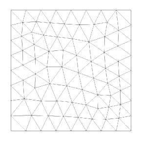
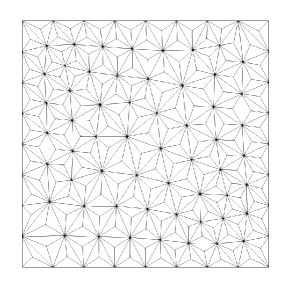
Figure 1: The coarsest mesh of the sequence of unstructured simplicial meshes is shown on the left, with mesh size $h=0.5$. To construct the second sequence of meshes we apply barycentric mesh refinement, resulting in the mesh on the right.

First, we aim to recreate the results obtained in [12], which use periodic boundary conditions. Then, we consider the case of the boundary condition used in this work, given by $\boldsymbol{\nu}\cdot\mathbf{u}=0$.

4.1 Periodic boundary

We aim to recreate the setting of numerical examples presented in [12]. While we will use the same setting of parameters, there are a few differences. The major difference is, that our formulation uses a slightly different damping term [26] than the one considered in [12]. Furthermore, in [12] quadrilatera meshes were considered, whereas we will use the simplicial meshes described in Figure 1. The setting is as follows: we consider as computational domain the square $(-4,4)^{2}$ with periodic boundary conditions, and a source term given by

$$s=(-i\omega+\partial_{\mathbf{b}})\begin{pmatrix}g\\ 0\end{pmatrix}$$ (28)

where $g(x,y)$ is the Gaussian given by $g(x,y)=\sqrt{a/\pi}\exp(-a(x^{2}+y^{2})).$ Here $a=\log(10^{6})$ such that $g$ is equal to $10^{-6}$ on the unit circle. The parameters are chosen as

$$\rho=1.5+0.2\cos(\pi x/4)\sin(\pi y/2), c_{s}^{2}=1.44+0.16\rho, \omega=0.78\times 2\pi,$$ (29)

$$\gamma=0.1, \Omega=(0,0), p=1.44\rho+0.08\rho^{2}.$$

and finally, the background flow is given by

$$\mathbf{b}=\frac{\alpha}{\rho}\begin{pmatrix}0.3+0.1\cos(\pi y/4)\\ 0.2+0.08\sin(\pi x/4)\end{pmatrix}$$ (30)

The error in the $\left\|\cdot\right\|_{\mathbb{X}}$-norm is considered against a reference solution computed with polynomial degree $k=5$ and mesh size $h=1.5\cdot 2^{-6}$. Plots of the reference solution are shown in Figure 4 (compare with [12, Fig. 8, 12]). In Figure 2 we compare convergence rates for $\alpha=0.1$, putting us safely into the regime of sub-sonic flow. We consider the two different types of mesh sequences for polynomial degrees $k=1,2,3,4.$ On unstructured meshes the error is given in Figure 2 on the left. There, we observe good convergence rates for $k=4$, after a pre-asymptotic phase, which might be caused by nearly singular vertices. For the meshes using barycentric refinement we observe convergence rates of order $\mathcal{O}(h^{k})$ for $k\geq 2$, aligning with Assumption 8, shown in Figure 2 in the center. We also show the error for the Taylor-Hood variant which we discussed in Remarks 15 and 21, in Figure 2 on the right. The method used an $H^{1}$ conforming choice for the space $Q_{n}$, and we use unstructured meshes. The method suffers from a long pre-asymptotic phase and shows a worse approximation error compared to the other two methods. The rates agree with Remark 14.

Figure 2: Convergence against a reference solution computed with polynomial degree $k=5$ and mesh size $h=1.5\cdot 2^{-6}$. We consider the setting described in (28) and (LABEL:eq:coeffs1) with periodic boundary conditions and fixed $\alpha=0.2$ for the background flow $\mathbf{b}$ given in (30), and different polynomial degree $k=1,2,3,4$ and varying mesh size. From left to right we consider: unstructured meshes, barycentric refined meshes, and the Taylor-Hood variant, i.e. unstructured meshes with $Q_{n}\subset H^{1}$. The error is measured in the $\left\|\cdot\right\|_{\mathbb{X}}$-norm.

In Figure 3 we compare different values of the coefficient for the background flow, $\alpha=0.2,0.5,1.5,3$, on the unstructured meshes. Assuming a good inf-sup constant of $\beta_{h}=0.5$ we have that the right hand side of our assumption on the Mach number in Theorem 20 is at best

$$\beta_{h}^{2}\frac{\underline{c_{s}}^{2}\underline{\rho}}{\overline{c_{s}}^{2}\overline{\rho}}\frac{1}{1+\tan^{2}\theta}\approx 0.06.$$ (31)

With the choice of $\alpha=3$, we exceed the upper bound notably, compare the values in Figure 3. The reference solution for $\alpha=0.2,1.5$ is presented in Figure 4. As the reference solution changes with $\alpha$, we additionally consider the consistency error, as in [12]. Let us denote

$$S_{1}=-\rho(\omega+i\partial_{\mathbf{b}}+i\Omega\times)^{2}\mathbf{u}-\gamma\rho i\omega\mathbf{u},\ S_{2}=\nabla\left(\rho c_{s}^{2}\operatorname{div}\mathbf{u}\right)-(\operatorname{div}\mathbf{u})\nabla p+\nabla(\nabla p\cdot\mathbf{u})-\operatorname{Hess}(p)\mathbf{u}$$

then the consistency error is given by

$$\text{consistency error}=\frac{\left\|S_{1}-S_{2}\right\|_{\mathbf{L}^{2}(\mathcal{O}\setminus B_{1.5})}}{\left\|S_{1}\right\|_{\mathbf{L}^{2}(\mathcal{O}\setminus B_{1.5})}}$$

where the error is measured on the domain without the disk with radius $1.5$ centered at the origin, denoted by $\mathcal{O}\setminus B_{1.5}$. Thus removing the effects of the source term $s$. We observe in Figure 3, that the error and the consistency error worsen considerably for $\alpha=1.5,3$ and an optimal rate of convergence is not visible for the considered mesh widths.

Figure 3: On unstructured meshes with periodic boundary conditions we consider the error in the $\left\|\cdot\right\|_{\mathbb{X}}$-norm (left) and consistency-error (right) against a reference solution for different values of the coefficient in the background flow $\mathbf{b}$, given in (30), and fixed polynomial order $k=4$.

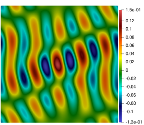
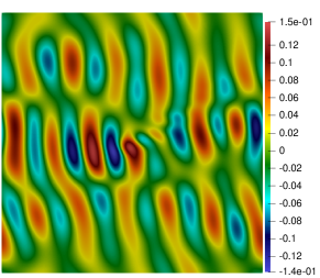
Figure 4: The real part of the first entry of the reference solution computed with $k=5$ and $h=1.5\cdot 2^{-6}$ for two different values of the coefficient of the flow field $\mathbf{b}$, $\alpha=0.2$ on the left and $\alpha=1.5$ on the right.

4.2 Normal boundary condition

In this section we are considering the boundary condition $\boldsymbol{\nu}\cdot\mathbf{u}=0$. We do not introduce a new finite element, instead we continue to use the finite element space defined in (27), and we incorporate the boundary condition using Nitsche’s method. Therefore, we add the following terms to (7)

$$-\langle c_{s}^{2}\rho\mathbf{u}\cdot\boldsymbol{\nu},\operatorname{div}\mathbf{u}^{\prime}\rangle_{\partial\mathcal{O}}-\langle c_{s}^{2}\rho\operatorname{div}\mathbf{u},\mathbf{u}^{\prime}\cdot\boldsymbol{\nu}\rangle_{\partial\mathcal{O}}+\frac{\lambda k^{2}}{h}\langle c_{s}^{2}\rho\mathbf{u}\cdot\boldsymbol{\nu},\mathbf{u}^{\prime}\cdot\boldsymbol{\nu}\rangle_{\partial\mathcal{O}}$$

where we choose $\lambda=2^{15}$. We again consider the domain $\mathcal{O}=(-4,4)^{2}$ and the parameters as in (LABEL:eq:coeffs1). Only the background flow is changed to satisfy $\mathbf{b}\cdot\boldsymbol{\nu}=0$ on $\partial\mathcal{O}$, and will now be given by

$$\mathbf{b}=\frac{\alpha}{\rho}\begin{pmatrix}\sin(\pi x)\cos(\pi y)\\ -\cos(\pi x)\sin(\pi y)\end{pmatrix}.$$ (32)

The flow additionally fulfills $\operatorname{div}(\rho\mathbf{b})=0$ in $\mathcal{O}$. In the following we will consider two examples with different source terms.

First, we consider convergence against a manufactured solution, by choosing the source term $s$ such that the solution will be given by

$$\frac{1}{\rho}\begin{pmatrix}(1+i)g\\ -(1+i)g\end{pmatrix}$$ (33)

where $g$ is again the Gaussian with $a=\log(10^{6})$. As $g$ equals $10^{-6}$ on the unit circle we can consider the boundary conditions fulfilled numerically to a reasonable degree. Results for fixed $\alpha=0.1$ are shown in Figure 5. We consider unstructured meshes and barycentric refined meshes. Further we include the Taylor-Hood variant outlined in Remarks 15 and 21 using unstructured meshes and an $H^{1}$ conforming choice for the space $Q_{n}$. For unstructured and barycentric refined meshes we observe the expected convergence rates for $k\geq 3$ and $k\geq 2$, respectively. The method with $Q_{n}\subset H^{1}$ shows again a long pre-asymptotic phase and a worse approximation error compared to the other two methods. Furthermore, for $k=3$ we only observe a long preasymptotic phase, optimal convergence rate is never reached.

Figure 5: Convergence towards an exact solution given in (33) for different polynomial orders $k=1,2,3,4$ for varying mesh sizes $h$. We consider homogeneous normal boundary contition with fixed $\alpha=0.1$ in the background flow $\mathbf{b}$, given in Equation 32. From left to right we consider: unstructured meshes, barycentric refined meshes, and unstructured meshes with $Q_{n}\subset H^{1}$. The error is measured in the $\left\|\cdot\right\|_{\mathbb{X}}$-norm.

Second, we consider again the source term given in (28), this time including the boundary condition, and compare against a reference solution, computed using $k=5$ and $h=2^{-4}$ in Figure 6. The first two plots in Figure 6 we fix $\alpha=0.1$ and consider two different mesh types. For both methods we observe good convergence rates of order $\mathcal{O}(h^{k})$, however, barycentric refinement show more stable rates and a better error overall. In Figure 6, on the right, we consider unstructured meshes, and different values of the coefficient $\alpha$ for for the flow given in (32). We choose $\alpha=0.1,0.2,0.3,0.4$ resulting in the corresponding Mach numbers $\left\|c_{s}^{-1}\mathbf{b}\right\|_{\mathbf{L}^{\infty}}^{2}\approx 2\mathrm{e}{-3},\ 0.01,\ 0.02,\ 0.04$. This can be compared to the example with periodic boundary conditions presented in Figure 3. Again, assuming an optimal inf-sup constant, the right hand side of our assumption on the Mach number in Theorem 20 is at best $\beta_{h}^{2}\frac{\underline{c_{s}}^{2}\underline{\rho}}{\overline{c_{s}}^{2}\overline{\rho}}\frac{1}{1+\tan^{2}\theta}\approx 0.06.$ Without the periodic boundary, we can see a loss in convergence set on earlier, at $\left\|c_{s}^{-1}\mathbf{b}\right\|_{\mathbf{L}^{\infty}}^{2}\approx 0.02$, most likely due to a worse discrete inf-sup constant.

Figure 6: Convergence against a reference solution on the unstructured meshes on the left and barycentric refined meshes in the middle, considering polynomial degree $k=1,2,3,4$. Here $\alpha=0.1$ and the background flow is as in (32). On the right we consider the unstructured meshes with $k=4$ and different background flows.

5 Conclusion

In this article we reported in Theorem 3 a new T-compatibility criterion to obtain the regularity of approximations. As an example of application we considered the damped time-harmonic Galbrun’s equation (which is used in asteroseismology) and we proved in Theorem 20 convergence for discretizations with divergence stable (Assumption 8) $\mathbf{H}^{1}$ finite elements. Although the results of this article constitute only a first step in the numerical analysis for the oscillations of stars. The subsonic Mach number assumption

$$\|c_{s}^{-1}\mathbf{b}\|_{\mathbf{L}^{\infty}}^{2}<\beta_{h}^{2}\frac{\underline{c_{s}}^{2}\underline{\rho}}{\overline{c_{s}}^{2}\overline{\rho}}$$ (34)

is far from being optimal. In stars the density decays with increasing radius and hence the ratio $\frac{\underline{c_{s}}^{2}\underline{\rho}}{\overline{c_{s}}^{2}\overline{\rho}}$ becomes very small. Thus a goal is to get rid of this factor in (34) by a more refined analysis or possibly by more sophisticated discretization methods. In addition it is desired to replace in (34) the discrete inf-sup constant of the divergence $\beta_{h}$ with a better constant closer to $1$. The reported computational examples serve only to illustrate the convergence of the finite element method and computational experiments with realistic parameters for stars are eligible. In particular, a numerical realization of a transparent boundary condition is necessary [22, 28, 4]. Finally we aim to apply the new T-compatibility technique to a number of equations/discretizations for which [21] is too rigid.

Appendix A Construction of $\mathbf{H}^{1}_{\boldsymbol{\nu}0}$-conforming finite element space

The convenient way to obtain a vectorial $\mathbf{H}^{1}$ finite element space is to use a scalar $H^{1}$ finite element space $Y_{n}$ and to use $(Y_{n})^{3}$. Hence if $u_{j}$ and $\mathrm{dof}_{j}(u)$ are the basis functions and degrees of freedom of $Y_{n}$, then $u_{j}\mathbf{e}_{l}$ and $\mathrm{dof}_{j}(\mathbf{e}_{l}\cdot\mathbf{u})$, $l=1,2,3$ with Cartesian unit vectors $\mathbf{e}_{j}$ are the basis functions and degrees of freedom of $(Y_{n})^{3}$. However, with this construction it is not clear how to handle the boundary condition $\boldsymbol{\nu}\cdot\mathbf{u}=0$ and hence the question how to construct finite element spaces of $\mathbf{H}^{1}_{\boldsymbol{\nu}0}$ remains. To solve this issue for each $j$ we reorganize $u_{j}\mathbf{e}_{l}$, $\mathrm{dof}_{j}(\mathbf{e}_{l}\cdot\mathbf{u})$, $l=1,2,3$ into tangential basis functions and DoFs $\mathbf{u}_{j}^{\mathrm{tan},l}$, $\mathrm{dof}_{j}^{\mathrm{tan}}$, $l=1,\dots,L_{j}$ and nontangential ones $\mathbf{u}_{j}^{\mathrm{nontan},l}$, $\mathrm{dof}_{j}^{\mathrm{nontan},l}$, $l=1,\dots,3-L_{j}$. Here $L_{j}=0$ if $\mathrm{dof}_{j}$ is a vertex DoF associated to a vertrex of $\partial\mathcal{O}$, $L_{j}=1$ if $\mathrm{dof}_{j}$ is a vertex or edge DoF associated to an edge of $\partial\mathcal{O}$, and $L_{j}=2$ if $\mathrm{dof}_{j}$ is a vertex, edge of face DoF associated to a face of $\partial\mathcal{O}$. Note that the tangential basis functions $\mathbf{u}_{j}^{\mathrm{tan},l}$ will satisfy $\boldsymbol{\nu}\cdot\mathbf{u}_{j}^{\mathrm{tan},l}=0$, whereas the nontangential basis functions $\mathbf{u}_{j}^{\mathrm{nontan},l}$ will in general satisfy neither $\boldsymbol{\nu}\times\mathbf{u}_{j}^{\mathrm{nontan},l}=0$ nor $\boldsymbol{\nu}\cdot\mathbf{u}_{j}^{\mathrm{nontan},l}=0$. However, $\boldsymbol{\nu}\cdot\mathbf{u}=0$ will imply $\mathrm{dof}_{j}^{\mathrm{nontan},l}(\mathbf{u})=0$. For $L_{j}=2$ we simply choose tangential vectors $\mathbf{t}_{1},\mathbf{t}_{2}$ and the normal vector $\boldsymbol{\nu}$ and set $\mathbf{u}_{j}^{\mathrm{tan},l}=u_{j}\mathbf{t}_{l}$, $\mathrm{dof}_{j}^{\mathrm{tan},l}(\mathbf{u}):=\mathrm{dof}_{j}(\mathbf{t}_{l}\cdot\mathbf{u})$, $l=1,2$ and $\mathbf{u}_{j}^{\mathrm{nontan,1}}=u_{j}\boldsymbol{\nu}$, $\mathrm{dof}_{j}^{\mathrm{nontan,1}}(\mathbf{u}):=\mathrm{dof}_{j}(\boldsymbol{\nu}\cdot\mathbf{u})$. For $L_{j}=1$ we choose the tangential vector $\mathbf{t}$ associated to the edge of $\partial\mathcal{O}$ and $\boldsymbol{\nu}_{1},\boldsymbol{\nu}_{2}$ as the normal vectors of the two adjacent faces. Thence we set $\mathbf{u}_{j}^{\mathrm{tan,1}}=u_{j}\mathbf{t}$, $\mathrm{dof}_{j}^{\mathrm{tan,1}}(\mathbf{u}):=\mathrm{dof}_{j}(\mathbf{t}\cdot\mathbf{u})$, $l=1,2$ and $\mathbf{u}_{j}^{\mathrm{nontan},l}=u_{j}\boldsymbol{\nu}_{l}$, $\mathrm{dof}_{j}^{\mathrm{nontan},l}(\mathbf{u}):=\mathrm{dof}_{j}(\boldsymbol{\nu}_{l}\cdot\mathbf{u})$, $l=1,2$. For $L_{j}=0$ there exist no tangential DoFs. Let $\boldsymbol{\nu}_{1},\boldsymbol{\nu}_{2},\boldsymbol{\nu}_{3}$ be the normal vectors of the three adjacent faces. Thence we set $\mathbf{u}_{j}^{\mathrm{nontan},l}=u_{j}\boldsymbol{\nu}_{l}$, $\mathrm{dof}_{j}^{\mathrm{nontan},l}(\mathbf{u}):=\mathrm{dof}_{j}(\boldsymbol{\nu}_{l}\cdot\mathbf{u})$, $l=1,2,3$. Thus to obtain a $\mathbf{H}^{1}_{\boldsymbol{\nu}0}$ conforming finite element space we simply set the DoFs associated to the nontangential DoFs to zero. Hence for $\mathbf{u}\in\mathbf{H}^{1}_{\boldsymbol{\nu}0}\cap\mathbf{H}^{s}$ the obtained finite element space has the same approximation properties as $(Y_{n})^{3}$.

References

- [1] G. Acosta, R. G. Durán and M. A. Muschietti, Solutions of the divergence operator on John domains, Adv. Math. 206 (2006) 373–401.
- [2] T. Alemán, M. Halla, C. Lehrenfeld and P. Stocker, Robust finite element discretizations for a simplified Galbrun’s equation, arXiv preprint arxiv:2205.15650 .
- [3] D. N. Arnold and J. Qin, Quadratic velocity/linear pressure stokes elements, in Advances in Computer Methods for Partial Differential Equations-VII, eds. R. Vichnevetsky, D. Knight and G. Richter (IMACS, 1992), pp. 28–34.
- [4] H. Barucq, F. Faucher, D. Fournier, L. Gizon and H. Pham, Outgoing modal solutions for Galbrun’s equation in helioseismology, J. Differ. Equations 286 (2021) 494–530.
- [5] S. Bertoluzza, The discrete commutator property of approximation spaces, C. R. Acad. Sci., Paris, Sér. I, Math. 329 (1999) 1097–1102.
- [6] D. Boffi, M. Costabel, M. Dauge, L. Demkowicz and R. Hiptmair, Discrete compactness for the -version of discrete differential forms, SIAM J. Numer. Anal. 49 (2011) 135–158.
- [7] A.-S. Bonnet-BenDhia, C. Carvalho and P. Ciarlet, Mesh requirements for the finite element approximation of problems with sign-changing coefficients, Numerische Mathematik 138 (2018) 801–838.
- [8] A.-S. Bonnet-BenDhia, J.-F. Mercier, F. Millot, S. Pernet and E. Peynaud, Time-harmonic acoustic scattering in a complex flow: A full coupling between acoustics and hydrodynamics, Communications in Computational Physics 11 (2012) 555–572.
- [9] K. Bredies, A variational weak weighted derivative: Sobolev spaces and degenerate elliptic equations, Report, 2008, https://imsc.uni-graz.at/bredies/papers/weighted_weak_derivative_elliptic.pdf.
- [10] A. Buffa, Remarks on the discretization of some noncoercive operator with applications to heterogeneous maxwell equations, SIAM Journal on Numerical Analysis 43 (2005) 1–18.
- [11] A. Buffa, M. Costabel and C. Schwab, Boundary element methods for Maxwell’s equations on non-smooth domains, Numer. Math. 92 (2002) 679–710.
- [12] J. Chabassier and M. Duruflé, Solving time-harmonic Galbrun’s equation with an arbitrary flow. Application to Helioseismology, Research Report RR-9192, INRIA Bordeaux, July 2018.
- [13] S. H. Christiansen and K. Hu, Generalized finite element systems for smooth differential forms and Stokes’ problem, Numer. Math. 140 (2018) 327–371.
- [14] R. S. Falk and M. Neilan, Stokes complexes and the construction of stable finite elements with pointwise mass conservation, SIAM J. Numer. Anal. 51 (2013) 1308–1326.
- [15] H. Galbrun, Propagation d’une onde sonore dans l’atmosphre et théorie des zones de silence (Gauthier-Villars, Paris, 1931).
- [16] J. Guzmán, A. Lischke and M. Neilan, Exact sequences on Powell-Sabin splits, Calcolo 57 (2020) 25, id/No 13.
- [17] J. Guzmán and M. Neilan, Inf-sup stable finite elements on barycentric refinements producing divergence-free approximations in arbitrary dimensions, SIAM J. Numer. Anal. 56 (2018) 2826–2844.
- [18] L. Hägg and M. Berggren, On the well-posedness of Galbrun’s equation, Journal de Mathématiques Pures et Appliquées 150 (2021) 112–133.
- [19] M. Halla, Analysis of radial complex scaling methods: scalar resonance problems, SIAM J. Numer. Anal. 59 (2021) 2054–2074.
- [20] M. Halla, Electromagnetic Steklov eigenvalues: approximation analysis, ESAIM, Math. Model. Numer. Anal. 55 (2021) 57–76.
- [21] M. Halla, Galerkin approximation of holomorphic eigenvalue problems: weak T-coercivity and T-compatibility, Numer. Math. 148 (2021) 387–407.
- [22] M. Halla, On the Treatment of Exterior Domains for the Time-Harmonic Equations of Stellar Oscillations, SIAM J. Math. Anal. 54 (2022) 5268–5290.
- [23] M. Halla, Analysis of radial complex scaling methods: scalar resonance problems, SIAM J. Numer. Anal. .
- [24] M. Halla, Convergence analysis of nonconform -finite elements for the damped time-harmonic Galbrun’s equation, arXiv preprint arxiv:2306.03496 .
- [25] M. Halla, On the approximation of dispersive electromagnetic eigenvalue problems in two dimensions, IMA J. Numer. Anal. 43 (2023) 535–559.
- [26] M. Halla and T. Hohage, On the well-posedness of the damped time-harmonic Galbrun equation and the equations of stellar oscillations, SIAM J. Math. Anal. 53 (2021) 4068–4095.
- [27] M. Halla, C. Lehrenfeld and P. Stocker, Replication Data for: A new T-compatibility condition and its application to the discretization of the damped time-harmonic Galbrun’s equation, GRO.data .
- [28] T. Hohage, C. Lehrenfeld and J. Preuß, Learned infinite elements, SIAM J. Sci. Comput. 43 (2021) a3552–a3579.
- [29] T. Hohage and L. Nannen, Convergence of infinite element methods for scalar waveguide problems, BIT 55 (2015) 215–254.
- [30] V. John, Finite element methods for incompressible flow problems, volume 51 of Springer Ser. Comput. Math. (Cham: Springer, 2016).
- [31] V. John, A. Linke, C. Merdon, M. Neilan and L. G. Rebholz, On the divergence constraint in mixed finite element methods for incompressible flows, SIAM Rev. 59 (2017) 492–544.
- [32] O. Karma, Approximation in eigenvalue problems for holomorphic Fredholm operator functions. I, Numer. Funct. Anal. Optim. 17 (1996) 365–387.
- [33] O. Karma, Approximation in eigenvalue problems for holomorphic Fredholm operator functions. II. (Convergence rate), Numer. Funct. Anal. Optim. 17 (1996) 389–408.
- [34] D. Lynden-Bell and J. P. Ostriker, On the stability of differentially rotating bodies, Monthly Notices of the Royal Astronomical Society 136 (1967) 293–310.
- [35] M. Maeder, G. Gabard and S. Marburg, 90 years of Galbrun’s equation: An unusual formulation for aeroacoustics and hydroacoustics in terms of the Lagrangian displacement, J. Theor. Comput. Acoust. 28.
- [36] M. Neilan, The Stokes complex: a review of exactly divergence-free finite element pairs for incompressible flows, in 75 years of mathematics of computation. Symposium celebrating 75 years of mathematics of computation, Institute for Computational and Experimental Research in Mathematics, ICERM, Providence, RI, USA, November 1–3, 2018 (Providence, RI: American Mathematical Society (AMS), 2020), pp. 141–158.
- [37] J. Schöberl, C++ 11 implementation of finite elements in ngsolve, Institute for analysis and scientific computing, Vienna University of Technology 30.
- [38] L. R. Scott and M. Vogelius, Norm estimates for a maximal right inverse of the divergence operator in spaces of piecewise polynomials, RAIRO, Modélisation Math. Anal. Numér. 19 (1985) 111–143.
- [39] F. Stummel, Diskrete Konvergenz linearer Operatoren. I, Math. Ann. 190 (1970/71) 45–92.
- [40] G. Unger, Convergence analysis of a Galerkin boundary element method for electromagnetic resonance problems, Partial Differ. Equ. Appl. 2 (2021) Paper No. 39.
- [41] G. Vainikko, Funktionalanalysis der Diskretisierungsmethoden (B. G. Teubner Verlag, Leipzig, 1976), mit Englischen und Russischen Zusammenfassungen, Teubner-Texte zur Mathematik.
- [42] S. Zhang, A new family of stable mixed finite elements for the 3d Stokes equations, Math. Comput. 74 (2005) 543–554.
- [43] S. Zhang, A family of 3d continuously differentiable finite elements on tetrahedral grids, Appl. Numer. Math. 59 (2009) 219–233.
- [44] S. Zhang, Divergence-free finite elements on tetrahedral grids for , Math. Comput. 80 (2011) 669–695.