Abstract.

We give an example of an eversion of the 2-sphere in the Euclidean 3-space, inspired by Morse theory, with a unique quadruple point. No homotopical tool is used.

1. Introduction

We recall that an eversion of the 2-sphere is a regular homotopy, that is path of immersions of the unit 2-sphere into $\mathbb{R}^{3}$, starting from the Identity map of the 2-sphere and ending to a map $S^{2}\to S^{2}$ reversing the orientation. If the normal orientation points outwards at the beginning of the path it points inwards in the end.

Figure 1. The trace of the homotopy from $S_{0}$ to $S_{1}$ on the plane $\{z=0\}$ will be contained in the gray rectangle.

Since the unexpected outstanding result etablished by S. Smale [4], many people gave examples of an eversion, including H. Hopf & N. Kuiper, A. Shapiro, M. Froissart, G. Francis & B. Morin, F. Apéry. The idea of Froissart-Morin, informally proved, circulated with the idea that there is a unique quadruple point along their eversion. That allowed J. Hughes [3] to prove that quadruple points are necessary in every path of immersions realizing an eversion of the 2-sphere. In 1994, Apéry [1] wrote a proof that there is a unique quadruple point in the Froissart-Morin eversion. More recently, A. Chéritat [2, 2014] proposed another sphere eversion that relies on the following property: namely, the space of $C^{1}$ immersions of $[0,1]$ to the square with fixed extremities and null winding number is contractible.

In the present note, we construct an eversion where each step is controlled by a few planar figures. First, we introduce two co-oriented surfaces $S_{0}$ and $S_{1}$ of revolution about the $x$-axis in $\mathbb{R}^{3}$. They are represented by their respective co-oriented planar sections which are drawn in Figure 1; $S_{0}$ is embedded and $S_{1}$ is immersed with a circle of double points.

The surface $S_{0}$ is isotopic to the unit 2-sphere with its outward co-orientation. It is easy to check $S_{1}$ is regularly homotopic to the unit 2-sphere with its inward co-orientation; indeed one cancel the circle of double points through the unique 3-ball whose angular boundary is contained in $S_{1}$.

We are going to prove the following proposition:

Proposition 1.1.

The co-oriented surfaces $S_{0}$ and $S_{1}$ are regularly homotopic through a homotopy with a unique quadruple point.

As a consequence, we have an eversion of the unit 2-sphere in $\mathbb{R}^{3}$ with a unique quadruple point.

Acknowledgements. In 2022, the interest to present a new example of a sphere eversion (if it is really new) is not clear. Being not a specialist, I did it for convincing myself this move of the 2-sphere really exists. Thanks to my former thesis advisor François Laudenbach, I got information from Tony Phillips who promptly sent references to us, in particular about the necessity of quadruple points. Then, François Apéry had long conversations with Laudenbach about the history of that topic. I am deeply grateful to all three of them.

2. Support, Movies and Routes

2.1.

The support of the regular homotopy from $S_{0}$ to $S_{1}$ that we are going to construct will be contained in a rectangular parallelepiped $W:=[0,2]\times[-6,6]\times[-6,6]$. The units on each axis are such that, for $i=0,1$, the boundary of $W\cap S_{i}$ is made of two squares. Moreover, $W\cap S_{i}$ is planar and parallel to $Oyz$ near its boundary .

Figure 2. The movie is continued symmetrically from $z=0$ to $z=2$.

Definition 2.2.

Given an immersed surface $S\subset\mathbb{R}^{3}$ such that $W\cap S$ satisfies the same boundary condition as $W\cap S_{0}$, the movie of $S$ is the family, parametrized by the Euclidean coordinate $z$ which plays the role of time, of the level sets of the height function $z|_{W\cap S}$.

In Figure 2, we show a few moments of the movie of $S_{0}$. For a convenient choice of the unit of the $z$-axis, the critical values of the height function of $S_{0}$ are $\pm 1$ and for $z\leq-2$ or $z\geq 2$ the level set is made of two parallel segments. The lower saddle point has the sign $+$ meaning that $\partial_{z}$ is an outward normal to $S_{0}$ at this point. The upper saddle point has the sign $-$.

In Figure 3, we present the movie of $S_{1}$ from time $z=-4$ to $z=0$; it is extended by symmetry with respect to the horizontal plane $z=0$ to the interval $[0,4]$. The critical values of the height function are still $z=\pm 1$. The lower saddle point has the sign $-$ and the upper saddle point has the sign $+$.

Figure 3. This movie is extended symmetrically from $z=0$ to $z=4$. Among the three double points at level $-1$, the saddle point is marked with a circle.

2.3.

The construction of the homotopy $(S_{t})_{t\in[0,1]}$ deals only with $W$ (the support of the desired regular homotopy) and is different in nature for $z\leq 2$ and $z\geq 2$. More precisely, the $z$ function, restricted to $S_{t}$, will have permanently two saddle points in $W$ and these critical points are moving in $W\cap\{z\leq 2\}$ only. For this part, it seems convenient to define the term of $route$. For short, in the remainder $S_{t}$ will denote what was previously noted $S_{t}\cap W$.

Definition 2.4.

A route $+$ (resp. $-$) is an embedded surface $R_{t}^{+}$ (resp. $R_{t}^{-}$), contained in $S_{t}$ with an octagonal boundary and which satisfies the following conditions.

1. the height function restricted to $S_{t}$ has a unique critical point in $R_{t}^{\pm}$ and that one is of type $\pm$.

2. The boundary $\partial R_{t}^{\pm}$ is made of:

   • two opposite sides named the lower sides which lie at some level $z_{0}$;

   • four vertical sides between the levels $z_{0}$ and $z_{0}+2$,

   • two sides of $R_{t}$ at level $z_{0}+2$ which are named the upper sides.

3. The projection to the plane $Oxy$ of the interior of $R_{t}^{\pm}$ is a diffeomorphism and the image of the octogon is a quadrilateral with cusps as vertices.

This definition remembers the Morse model except the verticality conditions.

2.5.

Two possibilities will be used for moving the routes and deforming $S_{t}$ in $W$:

• Vertically, $R_{t}^{\pm}$ is moved by an isometry where each point of $R_{t}^{\pm}$ remains on its own vertical line of $\mathbb{R}^{3}$.

• Horizontally, $R_{t}^{\pm}$ is moved by an isotopy in which each level set of $R_{t}^{\pm}$ moves at a constant level and the vertical sides of $\partial R_{t}^{\pm}$ are kept vertical.

For extending such a horizontal isotopy to a regular homotopy of $S_{t}\cap\{z\leq 2\}$ in $W\cap\{z\leq 2\}$ one has to remove some vertical rectangle swept out by one vertical side $A$ of $R_{t}^{\pm}$; at the same time, one glues some vertical rectangle swept out by another vertical side $A^{\prime}\neq A$ of $R_{t}^{\pm}$ so that, at each time $t\in[0,1]$, $S_{t}$ is a proper immersed surface in $W$ with a fixed boundary.

If $R_{t}^{\pm}$ moves vertically, $A$ is made of two horizontal arcs at the same level and $A^{\prime}$ as well with $A^{\prime}\cap A=\emptyset$ . Going down requiers some vertical room below $A$ for being swept out; and similarly for moving up.

Figure 4. View of a route $+$.

Figure 5. Projection to the plane $Oxy$ of a route $+$. The thin lines are the images of some level sets equipped with their ascending gradients.

The routes $-$ and $+$ have the same shape. Only the co-orientation is reversed; in other words, one turns Figure 4 upside down.

3. The regular homotopy for $z\leq 2$

A sequence of eleven figures is needed to describe successive steps of $S_{t}$ at times $t_{1}=0<t_{2}<\cdots<t_{11}=1$ and mainly at the level $z=0$ (thick plain lines); at every such a time, the projected routes to the plane $z=0$ are drawn. The route $+$ (resp. $-$) is drawn in red (resp. green). When it seems to be useful, some other level sets of the routes will be drawn with dashed lines for understanding how the two routes, and hence the surface $S_{t_{i}}$, $i=1,\ldots,10$, are located in the domain $z\in[-5,2]$.

3.1.

The first four figures. Figure 6 (1) summaries Figure 2. Here, the two routes projects identically to the plane $z=0$; the lower sides of the route $-$ (green) are exactly the upper sides of the route $+$ (red). That allows one to move the route $-$ horizontally to the position drawn in Figure 6 (2). The upper sides of $R^{-}_{t_{2}}$ are drawn with two dashed lines and lie at level $z=2$.

Figure 6. Here, the dashed lines are at level $z=2$.

From Figure 6 (2) to Figure 6 (3), some horizontal isotopy is performed until the projection of the green route avoids that of the red route. Its movement during the next step, from (3) to (4), is just a descending isotopy which is allowed since, at time $t_{3}$, the lower sides of the green route are disjoint from the red route and have vertical rectangles below them. The upper sides of $R^{-}_{t_{4}}$ lie at level 0. So, there are drawn with two plain lines.

3.2.

The next seven figures. The two routes remain disjoint and located between the level sets $z=-2$ and $z=0$, except when $t\in[t_{10},1]$—see the end of the present subsection. On Figure 7, for simplicity, the two routes are represented at each time $t_{i}$ by a thick colored plain line $L^{\pm}_{t_{i}}$, the sign recalling the one of the considered route. This line stands for the projection of the route $R^{\pm}_{t_{i}}$ to the plane $z=0$. The upper sides of $R^{\pm}_{t_{i}}$ are two lines essentially parallel to $L^{\pm}_{t_{i}}$ except near their extremities.

The regular homotopy $t\in[t_{4},t_{5}]\mapsto S_{t}$ keeps the two routes pointwise fixed and consists of pushing the finger from the left to the right on the left wall while the opposite movement is applied to the the right wall. At each time, the movie of $S_{t}$, $t\in[t_{4},t_{5}]$, is similar (that is, smoothly conjugate) to the beginning of Figure 3 (the first two steps), apart from the routes.

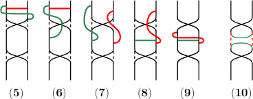
Figure 7. From $\bf(5)$ to $\bf(10)$ the dashed lines indicates the apparent contour of $S_{t}$ viewed from $z=\infty$. In $\bf(11)$ the drawing is like Figure 6; the red dashed lines show the lower sides of the red route, its upper sides coinciding with the green lines in $\{z=0\}$.

The steps from $t_{5}$ to $t_{10}$ need no special comments. Figures 7 (5) to 7 (10) are quite explicit for describing each movement. The last step, from (10) to (11), consists just of the series of three steps in Figure 6 performed backwards, up to intertwining the colors. The desired regular homotopy is now known in $W\cap\{z\leq 2\}$. $\Box$

For completing this homotopy to the missing part $W\cap\{2\leq z\leq 6\}$ (see section 4), it is useful to picture the two pathwise connected components of $S_{t}\cap\{z=2\}$. This is done in the next subsection.

3.3.

The two components of $S_{t_{i}}$, $i=5,...,11$, in level $z=2$.

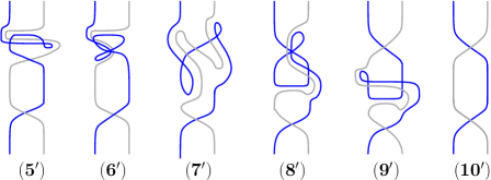
Figure 8. The two connected components, one in blue and the other in gray, of $S_{t}\cap\{z=2\}$ at the corresponding times of Figure 7.

The arcwise connected components of $S_{t}\cap\{z=2\}$ are easily deduced from the routes whose projection are drawn on Figures 6 and 7. The desired regular homotopy is now known in the domain $W\cap\{z\leq 2\}$. It will be completed in the next section.

4. Completing $S_{t}$ in $\{2\leq z\leq 6\}$

Let $P_{z}$ denote the horizontal plane $\mathbb{R}^{2}_{x,y}\times\{z\}$. We explain in Figure 9 how the movement is a function of time $t\in[0,1]$ depending on the interval in which $z$ is located, either $[2,3]$ (disjunction zone), $[3,5]$ (trivialization zone) or $[5,6]$ (isotopy zone). These different zones will be described in the remainder of the present section. The quadruple point will appear in the disjunction zone.

The intersection $S_{t}\cap P_{6}\cap W$ is made of two fixed parallel segments for every $t\in[0,1]$; that is one of the boundary conditions for gluing with the non-moving part of $S_{t}$. But the family $(S_{t})_{t}$, that will be built in each zone, does not exactly fulfill the right initial (resp. final) condition $S_{0}$ (resp. $S_{1}$) given in Figure 1. whose $z$-movies are given in Figures 2 and 3; both are slightly bashed up (see the $(x,y)$-boxes in Figure 9.) Nevertheless, a banal ambient isotopy, independent of $t$, rectifies this default. So, we neglect this phenomenon in the following discussion.

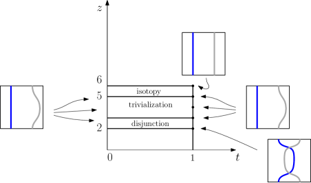
Figure 9. The boxes associated with some points in $(t,z)$-coordinates stand for $S_{t}\cap P_{z}\cap W$ equipped with $(x,y)$-coordinates.

4.1.

Disjunction zone. This zone corresponds to $z\in[2,3]$. Let $b_{t}$ and $g_{t}$ ($b$ like blue and $g$ like grey—see Figure 8) denote the two components at time $t$ of the curve $S_{t}\cap P_{2}\cap W$.

Claim. There exists an ambient isotopy $(\varphi^{t}_{\lambda})_{\lambda\in[0,1]}$ of $P_{2}$, supported in $P_{2}\cap int(W)$ and depending smoothly on $t$, which is viewed as an exernal parameter, such that $\varphi^{t}_{1}(g_{t})$ is disjoint from $b_{t^{\prime}}$ for every $t^{\prime}\in[0,1]$. Moreover, one may choose $(\varphi^{t}_{\lambda})$ such that the following holds:

1. The vector $\displaystyle{\frac{d\varphi^{t}_{\lambda}}{d\lambda}}$ points to the right of $\varphi^{t}_{\lambda}(g_{t})$ for every $(\lambda,t)\in[0,1]\times[0,1]$.

2. For $\lambda=1$, the curve $\varphi^{t}_{1}(g_{t})$ is independent of $t$ and denoted by $\gamma$.

3. The domain of $P_{2}\cap W$ to the left of $\gamma$ becomes convex after removing two strips $A^{-}$ and $A^{+}$, parallel to the $x$-axis, such that $g_{t}\cap A^{\pm}$ is independent of $t\in[0,1]$.
   

The third item imposed to $\gamma$ will be used for the construction in the trivialization zone.

Proof. For $t=0$, consider the one-dimensional foliation $\mathcal{F}_{0}$ parallel to the $x$-axis of the 2-dimensional domain $R_{0}$ in $P_{2}\cap W$ located to the right of the line $g_{0}$; orient $\mathcal{F}_{0}$ as the $x$-axis. Choose an arbirary ambient isotopy $(\rho_{t})_{t\in[0,1]}$ in $P_{2}$ supported in some compact set $C$ in $int(W)$ such that $\rho_{t}(g_{0})=g_{t}$. Then, we have an oriented foliation $\mathcal{F}_{t}:=(\rho_{t})_{*}(\mathcal{F}_{0})$ of $R_{t}:=\rho_{t}(R_{0})$. We impose the vector field $V^{t}$ to be tangent to $\mathcal{F}_{t}$ and point inwards $R_{t}$ along $g_{t}$ for every $t$. It remains to choose the velocity of the desired autonomous flow.

Consider the partial boundary $\Delta$ of $R_{0}$ made of the complete boundary $\partial R_{0}$ except the interior of the line $g_{0}$. There exists a collar $N$ of $\Delta$ in $R_{0}$ which fulfills the following two conditions for every $t\in[0,1]$:

1. $N\cap C=\emptyset$, that is, $N$ is kept pointwise fixed by $\rho_{t}$, and hence $N\subset R_{t}$.

2. $N$ is disjoint from $b_{t}$ for every $t\in[0,1]$.

Then $N$ is foliated by oriented segments parallel to the $x$-axis; this foliation is denoted by $\mathcal{F}_{N}$. One chooses a smooth path $\gamma$ in $N$, transverse to $\mathcal{F}_{N}$, joining the two end points of $g_{0}$ and having the same germ as $g_{0}$ near the end points. This arc $\gamma$ can be chosen so that item (3) of the claim holds.

Now, the vector field $V^{0}$ is chosen such that its flow, which reads

(4.1) $$\frac{d}{d\lambda}\varphi^{0}_{\lambda}(x,y)=V^{0}\bigl{(}\varphi^{0}_{\lambda}(x,y))\bigr{)},$$

maps $g_{0}$ to $\gamma$ in time 1. Then, if $V^{t}$ is the direct image of $V^{0}$ by $\rho_{t}:R_{0}\to R_{t}$, that is $V^{t}=\left(\rho_{t}\right)_{*}V^{0}$, its $\lambda$-flow $\varphi^{t}_{\lambda}$ also maps $g_{t}$ to $\gamma$ in time 1. That completes the proof of the claim. $\Box$

The surface $S_{t}\cap\{2\leq z\leq 3\}$ has two components that are built as follows: one is vertical over $b_{t}$ and the other intersects the plane $P_{z}$ along the curve $\varphi^{t}_{z-2}(g_{t})$ for every $t\in[0,1]$ and $z\in[2,3]$. Here, one uses the isotopy $\varphi^{t}_{\lambda}$ from the claim.

Since $g_{t}$ has no double point, a quadruple point only appears when $\varphi_{\lambda}(g_{t})$ meets a triple point of $b_{t}$. By Subsection 3.3, only $b_{t_{6}}$ and $b_{t_{9}}$ have triple points. Moreover, the triple point of $b_{t_{6}}$ already lies on the left of $g_{t_{6}}$. Since the isotopy $\varphi^{t_{6}}_{\lambda}$ constantly moves $g_{t_{6}}$ to its right, the triple point of $b_{t_{6}}$ is never overlapped by $\varphi^{t_{6}}_{\lambda}(g_{t_{6}})$. By the same argument, the triple point of $b_{t_{9}}$ is overlapped exactly once by $\varphi^{t_{9}}_{\lambda}(g_{t_{9}})$—see (9’) in Figure 8. So, there is exactly one quadruple point of the family $(S_{t})_{t}$ in the disjunction zone. Being careful in the other zones, no quadruple points will be created therein. $\Box$

4.2.

Trivialization zone. This zone is defined by $z\in[3,5]$; it is divided in two parts. Firstly, for $z\in[3,4]$ and $t\in[0,1]$, one applies to the blue line $b_{t}$ an ambient isotopy $(\psi^{t}_{\mu})_{\mu\in[0,1]}$ in the planar rectangle $P_{3}\cap W$ supported in the complement of the fixed grey line $\gamma=\varphi^{t}_{1}(g_{t})$ (see Claim from Subsection 4.1) and ending in the normalized position that is shown in Figure 10. The parameter of this isotopy is $\mu$ and $t$ is an external parameter.

The normalized blue line at time $t$ is contained in $P_{4}$ and denoted by $b^{\prime}_{t}$. Its main property is to be immersed and to have at most two critical points of the $y$-function restricted to $b^{\prime}_{t}$..

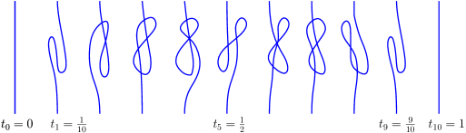
Figure 10. Here is a discrete $t$-movie in $P_{4}$ at times $t_{i}=\frac{i}{10}$, $i=0,1,\ldots,10$.

In the domain $\{3\leq z\leq 4\}\cap W$, the surface $S_{t}$ has one fixed component which is vertical over $\gamma$ and one moving component whose level set at time $t$ is the line $\psi^{t}_{z-3}(b_{t})\subset P_{z}$. The actual trivialization process starts from the normalized position in $\{z=4\}$ and consists of straightening $b^{\prime}_{t}$ smoothly in $t$. This will be performed in the next subsection.

4.3.

Actual trivialization process. One considers the family $(b^{\prime}_{t})_{t\in[0,1]}$ of lines in the plane $P_{4}$ from Figure 10. Note that this plane is canonically equipped with the $(x,y)$-coordinates of the box $W$ which carries the family $S_{t}$ of surfaces we are looking for. We choose a smooth parametrization of $b^{\prime}_{t}$

$$s\in[0,1]\mapsto\beta(s,t)=(x(s,t),y(s,t))\in P_{4}$$

satisfying the following requirements:

1. For every $t\in[0,1]$, the map $s\mapsto\beta(s,t)$ is an immersion.

2. The sign of the derivative $\partial_{s}y$ changes exactly at $s=\frac{1}{3}$ and $s=\frac{2}{3}$ for every $t\in\left[\frac{1}{10},\frac{9}{10}\right]$.

3. $\beta(s,\frac{9}{10})=\beta(s,\frac{1}{10})$.

In terms of these data, the trivialization is explicitely given by a barycentric combination formula that, for every $z\in[4,5]$, reads

(4.2) $$\left\{\begin{array}[]{lll}\hat{\beta}(z,s,t)&=(5-z)\beta(s,t)+(z-4)\beta(s,\frac{1}{10})\quad\text{if }t\in[\frac{1}{10},\frac{9}{10}]\\ &\\ &=\beta(s,t)\quad\text{ if }t\in[0,\frac{1}{10}]\cup[\frac{9}{10},1]\,.\end{array}\right.$$

Of course, these two formulas coincide in their common domains making their union continuous, but not smooth with respect to $t$. More precisely, the map $t\mapsto\hat{\beta}(-,-,t)$ is continuous with values in the space of $C^{1}$-functions of $(z,s)$, which is what we need. Nevertheless, the smoothing along $[4,5]\times\{\frac{i}{10}\}$, $i=1\text{ or }9$, is elementary, but useless.

If $z\in[4,5]$ and $t\in[\frac{1}{10},\frac{9}{10}]$ are fixed, then $s\mapsto\hat{\beta}(z,s,t)\in P_{z}$ is an immersion into $P_{z}$. Indeed, for $s\neq\frac{1}{3},\frac{2}{3}$ the partial derivative $\partial_{s}\hat{\beta}(z,s,t)$ does not vanish due to its $y$-component and, for $s=\frac{1}{3}\text{ or }\frac{2}{3}$, that is due to the $x$-component. In particular, for every fixed $t$ the map $(s,z)\in[0,1]\times[4,5]\mapsto(\hat{\beta}(f(z),s,t),z)$ parametrizes a proper immersed connected component of $S_{t}$ in $W\cap\{z\in[4,5]\}$ whatever the smooth function $f$. Here we use the convexity condition (3) in the claim of Subsection 4.1. There are also defaults of smoothness with respect to $z$ along the frontier between two consecutive zones. This will be answered in the next subsection. $\Box$

4.4.

Isotopy zone, end of the proof of Proposition 1.1. In the rectangle $P_{5}\cap W$, we see the following $t$-movie made of the gluing, rescaling and smoothing of the movie from 0 to $\frac{1}{10}$ and then the one from $\frac{9}{10}$ to 1. This consists a one-parameter family of proper curves in $P_{5}\cap W$ on which the $y$-coordinate has no critical points or a cancellable pair of critical points. Name $b^{\prime\prime}_{t}$ this blue curve at time $t$. For every $t\in[0,1]$, the path parametrized by $z\in[5,6]$ is the cancelling path issued from $b^{\prime\prime}_{t}$. At the same time, one can perform the straigthening of the corresponding grey curve.

We are now going to answer the smoothness question raised in the end of Subsection 4.3, which appears along $\{z=i\},\text{ for every }i=2,3,4,5$. The way of reasoning is independent of $i$. Near $i$, the variable $z$ will be replaced with $f(z)$ where $f$ is a $C^{\infty}$ function that is increasing, coincides with $Id$ far from $i$, fulfills $f(i)=i$ and all of whose derivatives vanish at $i$.

As mentioned in the beginning of Section 4, this finishes the proof of Proposition 1.1 and completes the example of sphere eversion we would like to explain.

References

- [1] Apéry F., Le retournement du cuboctaèdre, prépublication IRMA 1994/003, Université de Strasbourg.
- [2] Chéritat A., Yet another sphere eversion, arXiv:1410.4417[math.GT]2014.
- [3] Hughes J., Proof that every eversion of the sphere has a quadruple point, Amer. J. of Math. (1985), 501–505.
- [4] Smale S., A classification of immersions of the two-sphere, Trans. Amer. Math. Soc. 90 (1959), 281–290.