A Principled Evaluation Protocol for Comparative Investigation of the Effectiveness of DNN Classification Models on Similar-but-non-identical Datasets

Abstract

Deep Neural Network (DNN) models are increasingly evaluated using new replication test datasets, which have been carefully created to be similar to older and popular benchmark datasets. However, running counter to expectations, DNN classification models show significant, consistent, and largely unexplained degradation in accuracy on these replication test datasets. While the popular evaluation approach is to assess the accuracy of a model by making use of all the datapoints available in the respective test datasets, we argue that doing so hinders us from adequately capturing the behavior of DNN models and from having realistic expectations about their accuracy. Therefore, we propose a principled evaluation protocol that is suitable for performing comparative investigations of the accuracy of a DNN model on multiple test datasets, leveraging subsets of datapoints that can be selected using different criteria, including uncertainty-related information. By making use of this new evaluation protocol, we determined the accuracy of $564$ DNN models on both (1) the CIFAR-10 and ImageNet datasets and (2) their replication datasets. Our experimental results indicate that the observed accuracy degradation between established benchmark datasets and their replications is consistently lower (that is, models do perform better on the replication test datasets) than the accuracy degradation reported in published works, with these published works relying on conventional evaluation approaches that do not utilize uncertainty-related information.

1 Introduction

The purpose of evaluating trained machine learning models on held-out test datasets is to obtain unbiased estimates of their performance on datapoints that were not used for training purposes. A newer assessment approach in computer vision is to evaluate models on independent test datasets [1, 2] that have been created by carefully replicating the way older and highly popular datasets were constructed. We expect the accuracy on the replicated datasets to be similar to the accuracy on the original datasets. However, in reality, models suffer from a significant and consistent degradation in accuracy when evaluation is done using replicated datasets. For example, [1] created two test datasets, namely CIFAR-10.1 and ImageNetV2, by carefully following the way the CIFAR-10 [3] and ImageNet [4] datasets were constructed, respectively. They subsequently evaluated a large number of models on these test datasets and reported consistent and significant accuracy drops: $3\%-15\%$ on CIFAR-10.1 and $11\%-14\%$ on ImageNetV2. For convenience, in the remainder of this paper, we will refer to the original validation dataset partition of the ImageNet dataset as ImageNetV1.

Even though care is taken to ensure that the replicated datasets closely match their original datasets by design, it is reasonable to expect some characteristics of these datasets to still differ. Examples of factors that could account for such characteristic differences include: the under-representation of some sub-populations, unintended differences in sampling strategies [5], variation in the ratio of easy datapoints to difficult datapoints [1, 2], different degrees of label errors [6], and statistical bias during the replication process [7]. We conjecture that the degradation in the accuracy of a model on similar-but-non-identical test datasets does not necessarily indicate that the model fails to generalize well outside the training environment. Instead, there is a possibility that the adopted evaluation approaches do not adequately capture the rich information that DNN classification models generate.

DNN classification models generally produce a softmax vector. From this vector, we can extract two outputs for any given input datapoint – the predicted label and the corresponding predicted probability. The conventional approach for evaluating the accuracy of a model does not take into account the probabilities generated by the model, thereby treating every prediction equally. In this paper (see Section 2), we propose a principled evaluation protocol to assess the accuracy of a model on multiple similar-but-non-identical test datasets.

Consider a scenario where we seek to compare the accuracy of a model on two similar-but-non-identical test datasets. Instead of determining the accuracy using all the datapoints available in each dataset, we first create two subsets (one for each dataset), such that these two subsets match according to a particular matching criterion. We then evaluate the accuracy of the model on these two matched subsets. In this paper, the different matching criteria we study are ($i$) matching by both the predicted labels and their corresponding predicted probabilities and ($ii$) matching by the generated model probabilities.

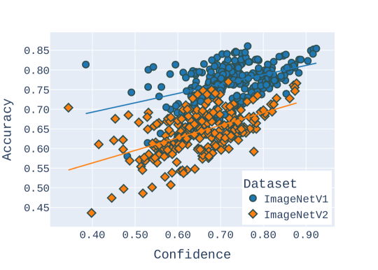
Figure 1: Scatter plot showing accuracy versus confidence for $286$ pre-trained ImageNet models. Each point corresponds to the accuracy and the confidence of a model on either the ImageNetV1 or ImageNetV2 dataset, with confidence denoting the average of the predicted probabilities for all datapoints.

Although it has been reported that the softmax probabilities generated by DNN models are usually over-confident [8, 9], there are research efforts [10, 11, 12] that acknowledge that softmax probabilities can serve as a baseline for the uncertainty estimates that models make about their predictions. We argue that these softmax probabilities can provide additional insight into the behavior of models that the use of zero-one loss or accuracy alone cannot capture; one such aspect is the relationship between the accuracy and the uncertainty of a model. A property of DNN models that is of high interest to practitioners is for a DNN model to be more correct when more certain and to be less correct when less certain. To observe the relationship between accuracy and confidence, we evaluated the accuracy and confidence of $286$ pre-trained ImageNet models on the ImageNetV1 and ImagenetV2 datasets. Figure 1 summarizes the obtained results by means of a scatter plot. Here, the confidence of a model is calculated as the average of the predicted probabilities associated with the predicted labels, for all the datapoints in the test dataset of interest. In Figure 1, we can observe that models generally tend to be less confident and less accurate on the ImageNetV2 dataset, whereas models tend to be more confident and more accurate on the original ImageNet validation set (ImageNetV1).

The aforementioned observation brings up interesting questions that warrant further investigation. Are the models signalling that the characteristics of the two datasets differ in more ways than we can explicitly model? Are pre-trained models too sensitive to their training settings which require that the training and test environments are independently and identically distributed ($i.i.d.$)? Using evaluation protocols that adequately capture the behavior of DNN models is a step forward towards finding answers to this kind of questions. The evaluation protocol that we introduce in this paper implicitly assesses how consistent the accuracy metric is with respect to the uncertainties generated by DNN classification models. For example, if we sample subsets of predictions with similar predicted probabilities (matched by predicted probabilities) from two test datasets, how large will the accuracy gap between these subsets be? Intuitively, we expect such a gap to be narrow ($i$) if the probabilities carry important information about the uncertainty (or confidence) that the model has on its predictions and ($ii$) if the uncertainty information correlates well with the accuracy metric. Indeed, our extensive evaluations of $278$ CIFAR-10 models and $286$ ImageNet models, as presented in Section 4, provide compelling evidence for the utility of our evaluation approach. In particular, if we leverage the uncertainty-related information generated by models, we find that the degradation in accuracy across all evaluated models may not be as large as has been previously reported.

The contributions of this paper are as follows:

1. we draw attention to a weakness when comparing the accuracy of models on multiple similar-but-non-identical datasets;

2. we propose a principled evaluation protocol for investigating the accuracy of models on multiple test datasets, with this evaluation protocol taking into account both the predicted labels and the predicted probabilities that are generated by models, thus allowing for more nuanced interpretation of model behavior; and

3. by evaluating $564$ pre-trained DNN models, we provide empirical evidence that indicates that the deterioration in accuracy may not be as bad as has been reported before, if we leverage the uncertainty-related information generated by DNN models.

In the remainder of this paper, we describe our principled evaluation protocol in detail in Section 2. Furthermore, we summarize related research efforts in Section 3. Next, we discuss our experimental setup and our experimental results in Section 4. Finally, we present our conclusions and a number of directions for future research in Section 5.

2 Proposed Evaluation Protocol

2.1 Background

In this section, we describe our principled evaluation protocol, which enables us to gain more insight into the performance of models when evaluation is done using multiple datasets. Although the newly introduced protocol could be used to evaluate any supervised classification model that generates predicted labels and their corresponding probabilities, in this paper, we restrict our scope to supervised DNN classification models for computer vision. In machine learning, supervised classification involves observing several examples of a random vector $\bm{X}$ and an associated random variable $Y$, with the aim of learning to predict $Y$ from $\bm{X}$. This is usually done by estimating the conditional probability distribution $P(Y|\bm{X})$ [13]. The formulation of our evaluation protocol assumes that we are provided with:

• an $i.i.d.$ dataset $\mathcal{D}=\{(\displaystyle{\bm{x}}^{(i)},y^{(i)})\}_{i=1}^{N}\subset\mathcal{X\times Y}$, which is further partitioned into disjoint train ($\mathcal{D_{\mathrm{train}}}$), validation ($\mathcal{D_{\mathrm{val}}}$), and test ($\mathcal{D_{\mathrm{test1}}}$) datasets, where $\mathcal{X}$ and $\mathcal{Y}=\{1,2,...,K\}$ denote the input space and label space, respectively, and where $K$ represents the number of classes, labels, or categories that each realization of $\bm{X}$ can be assigned to. An example input space may comprise a set of raw images belonging to the categories (denoted by integers) in a given label space;

• a classification model $f_{\bm{\theta}}:\mathcal{X}\to\mathcal{Y}$ with trained parameters $\bm{\theta}$. This classification model, which has been trained on $\mathcal{D_{\mathrm{train}}}$ and validated on $\mathcal{D_{\mathrm{val}}}$, produces the predicted class label $\hat{y}=\operatorname*{arg\,max}_{y\in\mathcal{Y}}P(Y=y|\bm{X}=\displaystyle{\bm{x}},\bm{\theta}$) and the corresponding predicted probability $\hat{p}=\max_{y\in\mathcal{Y}}P(Y=y|\bm{X}=\displaystyle{\bm{x}},\bm{\theta}$); and

• a second test dataset, $\mathcal{D_{\mathrm{test2}}}=\{(\displaystyle{\bm{x}}^{(i)},y^{(i)})\}_{i=1}^{M}\subset\mathcal{X\times Y}$, such that $\mathcal{D}\cap\mathcal{D_{\mathrm{test2}}}=\emptyset$.

• an $i.i.d.$ dataset $\mathcal{D}=\{(\displaystyle{\bm{x}}^{(i)},y^{(i)})\}_{i=1}^{N}\subset\mathcal{X\times Y}$, which is further partitioned into disjoint train ($\mathcal{D_{\mathrm{train}}}$), validation ($\mathcal{D_{\mathrm{val}}}$), and test ($\mathcal{D_{\mathrm{test1}}}$) datasets, where $\mathcal{X}$ and $\mathcal{Y}=\{1,2,...,K\}$ denote the input space and label space, respectively, and where $K$ represents the number of classes, labels, or categories that each realization of $\bm{X}$ can be assigned to. An example input space may comprise a set of raw images belonging to the categories (denoted by integers) in a given label space;

• a classification model $f_{\bm{\theta}}:\mathcal{X}\to\mathcal{Y}$ with trained parameters $\bm{\theta}$. This classification model, which has been trained on $\mathcal{D_{\mathrm{train}}}$ and validated on $\mathcal{D_{\mathrm{val}}}$, produces the predicted class label $\hat{y}=\operatorname*{arg\,max}_{y\in\mathcal{Y}}P(Y=y|\bm{X}=\displaystyle{\bm{x}},\bm{\theta}$) and the corresponding predicted probability $\hat{p}=\max_{y\in\mathcal{Y}}P(Y=y|\bm{X}=\displaystyle{\bm{x}},\bm{\theta}$); and

• a second test dataset, $\mathcal{D_{\mathrm{test2}}}=\{(\displaystyle{\bm{x}}^{(i)},y^{(i)})\}_{i=1}^{M}\subset\mathcal{X\times Y}$, such that $\mathcal{D}\cap\mathcal{D_{\mathrm{test2}}}=\emptyset$.

Algorithm 1 Strategy for matching two datasets based on both the predicted labels and probabilities of a model

procedure MatchPredictions($f_{\bm{\theta}}$, $\mathcal{D_{\mathrm{src}}}$, $\mathcal{D_{\mathrm{tgt}}}$, $\epsilon$)

     $\mathcal{P}_{\mathrm{src}}\leftarrow\textsc{Predict}(f_{\bm{\theta}},\mathcal{D_{\mathrm{src}}})$

     $\mathcal{P}_{\mathrm{tgt}}\leftarrow\textsc{Predict}(f_{\bm{\theta}},\mathcal{D_{\mathrm{tgt}}})$

     Initialize 3 empty arrays:

     $\mathcal{P}_{\mathrm{src\_matched}}$ = [ ]

     $\mathcal{P}_{\mathrm{tgt\_matched}}$ = [ ]

     $\mathcal{P}_{\mathrm{tgt\_unmatched}}$ = [ ]

     $N\leftarrow\textsc{Length}(\mathcal{P}_{\mathrm{tgt}})$

     for $i\leftarrow 1,N$ do

         $y_{t},\hat{y}_{t},\hat{p}_{t}\leftarrow\mathcal{P}_{\mathrm{tgt}}[i]$

         $y_{s},\hat{y}_{s},\hat{p}_{s},is\_match\leftarrow\textsc{Match}(y_{t},\hat{y}_{t},\hat{p}_{t},\mathcal{P}_{\mathrm{src}},\epsilon)$

         if $is\_match$ then

              $\mathcal{P}_{\mathrm{src\_matched}}.append((y_{s},\hat{y}_{s},\hat{p}_{s}))$

              $\mathcal{P}_{\mathrm{tgt\_matched}}.append((y_{t},\hat{y}_{t},\hat{p}_{t}))$

         else

              $\mathcal{P}_{\mathrm{tgt\_unmatched}}.append((y_{t},\hat{y}_{t},\hat{p}_{t}))$

         end if

     end forreturn $\mathcal{P}_{\mathrm{src\_matched}},\mathcal{P}_{\mathrm{tgt\_matched}},\mathcal{P}_{\mathrm{tgt\_unmatched}}$

end procedure

function Match($y_{t},\hat{y}_{t},\hat{p}_{t},\mathcal{P}_{\mathrm{src}},\epsilon$)

     Initialize an empty $\mathcal{P}_{\mathrm{matched}}$ = [ ]

     for all $(y,\hat{y},\hat{p})\in\mathcal{P}_{\mathrm{src}}$ do

         if $\hat{y}_{t}=\hat{y}$ and $\hat{p}_{t}\in[\hat{p}-\epsilon,\hat{p}+\epsilon]$ then

              $\mathcal{P}_{\mathrm{matched}}.append((y,\hat{y},\hat{p}))$

         end if

     end for

     if |$\mathcal{P}_{\mathrm{matched}}$| > 0 then

         $(y_{s},\hat{y}_{s},\hat{p}_{s})\leftarrow\textsc{RandomSelect}(\mathcal{P}_{\mathrm{matched}})$

         $\mathcal{P}_{\mathrm{src}}.remove((y,\hat{y},\hat{p}))$

         return $(y_{s},\hat{y}_{s},\hat{p}_{s},is\_match)$

     else

         return $(0,0,0,False)$

     end if

end function
$\triangleright$ The Predict(.) function returns the predictions of a model in an array that consists of tuples $(y,\hat{y},\hat{p})$, where $y$, $\hat{y}$, and $\hat{p}$ denote the ground truth label, the predicted label, and the predicted probability, respectively.
$\triangleright$ The RandomSelect(.) function returns a randomly selected tuple $(y,\hat{y},\hat{p})$ from the array that contains the input tuples.
$\triangleright$ The $\mathcal{P}_{\mathrm{src}}.remove((y,\hat{y},\hat{p}))$ in RandomSelect(.) accounts for random selection without replacement.

The task at hand is to compare the effectiveness of $f{{}_{\bm{\theta}}}$ on $\mathcal{D}_{\mathrm{test1}}$ and $\mathcal{D_{\mathrm{test2}}}$ using certain metrics, such as accuracy.

2.2 Matching by Predicted Labels and Probabilities

In Section 1, we introduced two matching criteria: ($i$) matching by both the predicted labels and their corresponding predicted probabilities and ($ii$) matching by the predicted probabilities only. In what follows, we provide the description of our proposed evaluation protocol based on the first matching criterion, i.e., matching by both the predicted labels and their corresponding predicted probabilities. Given two test datasets $\mathcal{D_{\mathrm{test1}}}$ and $\mathcal{D_{\mathrm{test2}}}$, our evaluation strategy aims at assessing the accuracy of a model on these datasets, while taking into account the predicted probabilities generated by this model. For convenience, we designate the dataset with the larger number of datapoints as the source dataset $\mathcal{D_{\mathrm{src}}}$, and the other dataset as the target dataset $\mathcal{D_{\mathrm{tgt}}}$.

First, the model of interest is used to generate the predicted labels and probabilities for all the datapoints in both test datasets. We represent the output of the model, for a datapoint, as a tuple $(y,\hat{y},\hat{p})$, where $y$, $\hat{y}$, and $\hat{p}$ represent the ground truth label, the predicted label, and the predicted probability, respectively. In a next step, we generate the subsets $\mathcal{P_{\mathrm{src}}}$ and $\mathcal{P_{\mathrm{tgt}}}$, whose elements are tuples $(y,\hat{y},\hat{p})$, by sub-sampling from all the model outputs obtained for the datasets $\mathcal{D_{\mathrm{src}}}$ and $\mathcal{D_{\mathrm{tgt}}}$, making use of predefined matching criteria. Our first matching criterion is summarized as follows: for every element in $\mathcal{P_{\mathrm{tgt}}}$, find an element in $\mathcal{P_{\mathrm{src}}}$, such that they both have the same predicted labels and such that their predicted probabilities are approximately equal. In this context, we make use of a very small fraction $\epsilon$ to control how approximately matched the probability values should be. For example, if we want the probability difference to be within $\pm 1\%$, we set $\epsilon=0.01$. Our evaluation protocol, using this matching criterion, is described in more detail in Algorithm 1 and a summarizing overview is presented in Figure 2. The description of our evaluation protocol, using the second matching criterion – matching by predicted probabilities only – is described in Algorithm 2 in Appendix A.3.

2.3 Accuracy Evaluation

The outputs generated by Algorithm 1 and Algorithm 2 are arrays: $\mathcal{P}_{\mathrm{src\_matched}},$ $\mathcal{P}_{\mathrm{tgt\_matched}}$, and $\mathcal{P}_{\mathrm{tgt\_unmatched}}$. We could also generate the source datapoints that remain unmatched. However, since the source dataset is mostly the $i.i.d.$ test dataset in our experiments and since our goal is to investigate the accuracy drop in the target dataset (the replicate dataset), we excluded the unmatched source datapoints from further analysis. The $\mathcal{P}_{\mathrm{src\_matched}}$ and $\mathcal{P}_{\mathrm{tgt\_matched}}$ arrays contain information about the model outputs that meet the matching criteria, while the $\mathcal{P}_{\mathrm{tgt\_unmatched}}$ array contains information about the model outputs that do not meet the matching criteria (i.e., for the datapoints in $\mathcal{D_{\mathrm{tgt}}}$ that do not have corresponding matching datapoints in $\mathcal{D_{\mathrm{src}}}$).

Although many other metrics can be used to evaluate the aforementioned arrays to get a better understanding of the datapoints that are considered similar or not similar, as judged by the outputs of a model, the scope of this paper is restricted to the accuracy metric, given that this metric is widely used for evaluating models on multiple test datasets. Our definition of accuracy is conventional – the ratio of the number of correctly classified datapoints to the total number of datapoints under evaluation. However, we make a distinction between accuracy evaluated on all the datapoints in a source or target dataset, and the accuracy evaluated on the matched datapoints. We refer to the former as simply accuracy and to the latter as matched accuracy.

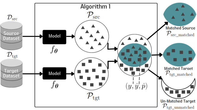
Figure 2: Visual overview of the matching strategy described by Algorithm 1.

3 Related Research

In this section, we briefly summarize research efforts that are related to our work.

Possible Explanations for the Accuracy Degradation in Replication Datasets.

Even after carefully following the way the original datasets were constructed, the creators of the CIFAR-10.1 and the ImageNetV2 datasets [1] concluded that the degradation in accuracy is not resulting from adaptive over-fitting to the original test datasets, suggesting that a possible explanation for the degradation is the presence of harder-to-classify images in the newer test datasets. [7] concluded that the accuracy degradation in the ImageNetV2 dataset is the result of statistical bias in the creation of the ImageNetV2 dataset. They show that the accuracy gap is indeed narrower if various sources of statistical bias are accounted for. Specifically, they demonstrate that only $3.6\%\pm 1.5\%$ of the accuracy drop for ImageNetV2 remains unaccounted for. Our experimental results support their finding and our proposed evaluation protocol additionally provides a practical tool for realistic performance assessment of DNN models on multiple test datasets.

Softmax as Baseline for DNN Model Uncertainty.

There are studies that consider softmax outputs as approximations to the probabilities that are generated by DNN classification models: the use of softmax outputs has been considered as a baseline for detecting misclassified and out-of-distribution datapoints by [10], and has been demonstrated to be decent at capturing the uncertainty in the predictions produced by DNN models [11, 12]. Our principled evaluation approach and our empirical evaluation results lend support to the use of softmax outputs as a baseline for uncertainty estimation. However, we also align with other works [8, 9] that call for caution in the interpretation of softmax outputs as confidence values or probabilities that models have about their predictions, since models are prone to over-confidence. Although well-calibrated probabilities are desirable, our approach is not explicitly aimed at evaluating how calibrated the probabilities are. We aim at investigating how consistent the outputs of a model are. For example, a model that is over-confident but also consistent in multiple environments could still be useful for downstream pipelines, and the probabilities generated by the model could be further calibrated.

Calibration of Models.

Model calibration or confidence calibration is the problem of predicting probability estimates that are representative of the true correctness likelihood [8]. Published methods for model calibration involve improving the modeling process [14, 15, 11, 16, 17], thereby creating models that inherently produce calibrated probabilities, or utilizing post-processing techniques to improve the outputs of already trained models [18, 8]. The Expected Calibration Error [18, 8] is a popular metric for evaluating how calibrated models are. Although popular, the ECE has a number of weaknesses: ($i$) given that ECE is histogram-based, it heavily depends on the binning strategy used [19, 20]; ($ii$) the predicted probabilities generated by different models for the same dataset could have different densities, hence making the ECE not the ideal metric for comparing the calibration of a model on different datasets; and ($iii$) ECE is independent of accuracy, which means that a model could be calibrated but have low accuracy, and vice versa, which implies the existence of a trade-off between accuracy and calibration. Our evaluation approach jointly evaluates the accuracy and consistency of the predicted probabilities in relation to accuracy, thereby enabling an effective evaluation of a model on multiple similar-but-non-identical datasets.

Classification with a Reject Option.

Classifiers with a reject option can abstain from predicting a label if certain criteria are not met. Examples of classifiers with a reject option are those where the rejection is based on confidence thresholds [21, 22]. This group of classifiers comes with a trade-off between error rates and rejection rates, benefiting from reliable confidence estimation. Whereas research efforts on classification with a reject option aim at creating classifiers that have improved effectiveness while being able to abstain from making certain predictions, the aim of our work is to evaluate any DNN classification model in a principled manner. This is even more crucial when evaluating a model under different settings.

4 Experimental Setup and Results

4.1 Experimental Setup

Dataset Pairs

: The goal of our experiments is to evaluate a representative sample of published DNN classification models on the CIFAR-10 and ImageNet datasets, using the evaluation protocol proposed in Section 2. To that end, we trained $278$ models on the CIFAR-10 dataset using PyTorch implementations by [11] under various training settings. These training settings include different model architectures, loss functions, learning rate schedules, data augmentation techniques, and random seeds. We describe the datasets used in Table 1 in Appendix A.1 and we list the various characteristics of the trained models in Table 2 in Appendix A.2. For CIFAR-10, evaluations are carried out on the following test dataset pairs: ($i$) CIFAR-10 versus CIFAR-10.1, ($ii$) CIFAR-10 versus CIFAR-10.2, and ($iii$) CIFAR-10 versus CINIC-10. The CIFAR-10.2 dataset was created by [2] and is a variant of the CIFAR-10 dataset; it was derived from the same source as CIFAR-10 and assembled via a similar process. The CINIC-10 dataset[23] was derived from ImageNet, and consists of images that belong to the same classes as those of the CIFAR-10 dataset; all the images where resized to the resolution of $32$$\times$$32$.

Due to computational limitations, we did not re-train the ImageNet models but utilized $286$ pre-trained published models from a popular PyTorch repository [24]. The network architectures of the pre-trained ImageNet models and their names, as used in the source GitHub repository, are presented in Table 3 in Appendix A.2. Similar to what was done for the CIFAR-10 pairs, we determine the accuracy and matched accuracy for the ImageNetV1 versus ImageNetV2 dataset pair for each pre-trained model. The ImageNetV1 dataset consists of a total of $50,000$ images taken from $1,000$ categories, while ImageNetV2 consists of a total of $10,000$ images taken from $1000$ categories.

Generated Results.

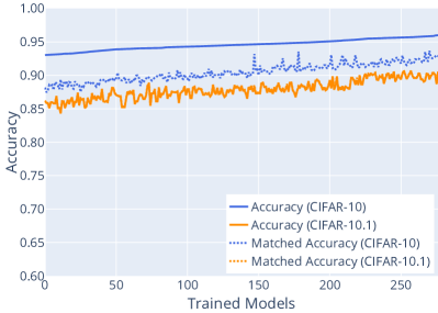
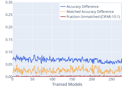
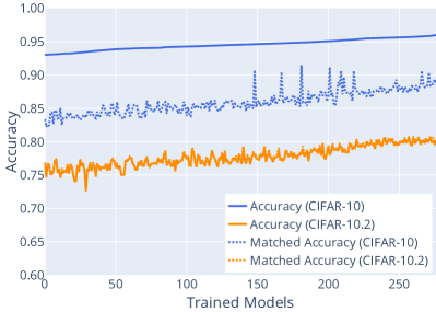
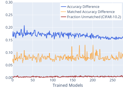
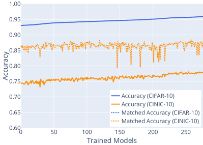
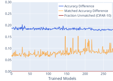
Figure 6: Plots for accuracy and matched accuracy, when matched by predicted probabilities only for the following dataset pairs: (a) CIFAR-10 versus CIFAR-10.1, (c) CIFAR-10 versus CIFAR-10.2, and (e) CIFAR-10 versus CINIC-10. Plots for accuracy difference, matched accuracy difference, and fraction unmatched for (b) CIFAR-10 versus CIFAR-10.1, (d) CIFAR-10 versus CIFAR-10.2, and (f) CIFAR-10 versus CINIC-10. The models in all plots are sorted according to increasing accuracy on CIFAR-10.

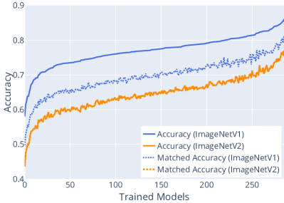
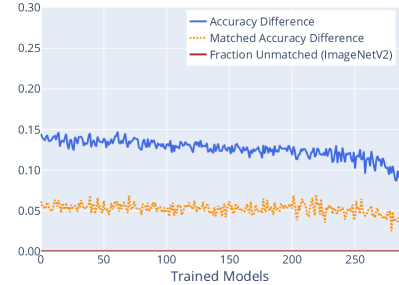
Figure 7: (a) Accuracy and matched accuracy plots and (b) difference in accuracy and matched accuracy for all models for the ImageNet and ImageNetV2 dataset pair. The models on all plots are sorted according to increasing accuracy on ImageNetV1.

We applied Algorithm 1 and Algorithm 2 to each of the aforementioned dataset pairs to generate matching subsets, with $\epsilon=0.005$. Subsequently, each model is evaluated on these subsets to determine ($i$) the accuracy on the source and the target datasets and ($ii$) the matched accuracy on the matched source and matched target datasets. Another value calculated is the fraction of datapoints in the target dataset that do not find a match with datapoints in the source dataset, which we refer to as Fraction Unmatched. These results are presented in Figure 3 and Figure 4. Additional results can be found in Figure 6 and Figure 7 in Appendix A.4. The accuracy and matched accuracy gaps are better visualized in the plots on the right column of these Figures. The results for the matched accuracy are the average of 10 runs of each algorithm (Algorithm 1 and Algorithm 2). Since the standard errors over these runs were negligible, we did not include error bars for the matched accuracy. For accuracy, we evaluate already trained models and it is not feasible to have the same pre-trained models over multiple seeds. Therefore, we plot the accuracy of the available pre-trained models.

[] [][] [][] []

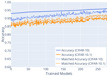
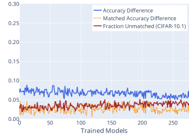
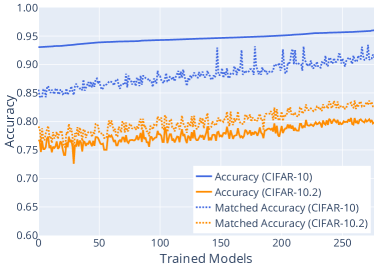
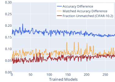
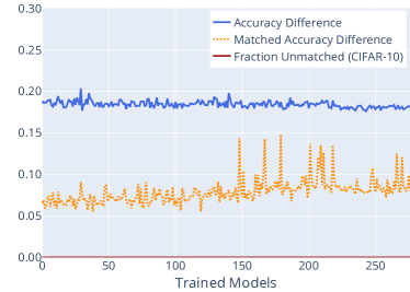
Figure 3: Plots for the accuracy and matched accuracy for (a) CIFAR-10 versus CIFAR-10.1, (c) CIFAR-10 versus CIFAR-10.2, and (e) CIFAR-10 versus CINIC-10. Plots for accuracy difference, matched accuracy difference, and fraction unmatched for (b) CIFAR-10 versus CIFAR-10.1, (d) CIFAR-10 versus CIFAR-10.2, and (f) CIFAR-10 versus CINIC-10. The models in all plots are sorted according to increasing accuracy on CIFAR-10.

[] []

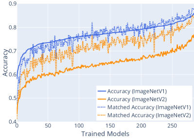
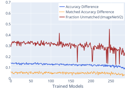
Figure 4: (a) Accuracy and matched accuracy plots and (b) difference in accuracy and matched accuracy for $286$ models evaluated on the ImageNet and ImageNetV2 dataset pair according to Algorithm 1. The models in all plots are sorted according to increasing accuracy on ImageNetV1.

4.2 Results and Discussion

Consistent and Significant Accuracy Drops.

Our extensive evaluation of the accuracy of a plethora of models, on both the original and replication datasets, produced results that are in line with the results reported by [1], [25], and [2]. When accuracy is evaluated on all datapoints, we observe consistent but significant accuracy drops on the replicated datasets. These results are shown in Figures 3, 3, 3, and 4 as the gap between the solid blue line and the solid orange line; the difference in accuracy can be better viewed in the corresponding accuracy difference plots in Figures 3, 3, 3, and 4 as the blue line.

Narrower Matched Accuracy Gaps.

Given an input image, a model is used to predict the label for this image and the likelihood of the correctness of the prediction, which we loosely interpret as the belief of the model about the correctness of the prediction. Algorithm 1 enables us to effectively partition the evaluation datasets into matching and non-matching subsets and to evaluate the consistency of the accuracy of models with respect to uncertainty.

By utilizing our evaluation protocol, which allows taking into account uncertainty information, the matched accuracy gap is consistently narrower, indicating that the accuracy of the models on the test dataset pairs are closer if the uncertainty information is taken into account. The key takeaway message here is that the uncertainty that models generates provide additional information that should be taken into to better evaluate the models. These results are presented in Figures 3, 3, 3, and 4 as the gap between the dotted blue line and the dotted orange line; the accuracy difference can better be viewed in Figures  3, 3, 3, and 4 as the orange line. The evaluation results obtained when matching is done by predicted probabilities only (our second matching criterion) can be found in Figures 6 and 7 in Appendix A.3.

Consistency of Confidence versus Accuracy across Various Subsets of the Test Datasets.

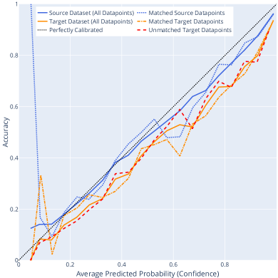
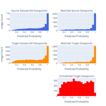
Figure 8: The plots of two characteristic of a pre-trained ResNet18 (swsl_resnet18) model [24] when evaluated on various subsets of the ImageNetV1 and ImageNetV2 datasets, as generated by our proposed evaluation protocol: (a) Accuracy versus Confidence and (b) Density plots for predicted probabilities.

To further illustrate the behavior of models for the various dataset subsets, we present in Figure 5 the accuracy versus confidence curves, which are also known as calibration curves or reliability diagrams [26], for all the subsets of the ImageNetV1 and the ImageNetV2 datasets. The predictions were generated by utilizing our proposed protocol to evaluate a pre-trained ResNext101 [27] ImageNet model. In Figure 5, we show the density plots for the predicted probabilities. The accuracy gap and the matched accuracy gap are $8.6\%$ and $3.1\%$, respectively, while the accuracy on the unmatched datapoints is $45.54\%$. These results primarily demonstrate that the accuracy obtained for different test sets can vary widely if some of their characteristics differ. However, the model behavior within these subsets is fairly consistent with respect to the correlation between the uncertainty values it generates and the accuracy for its predictions. This has practical implications: the performance of a deployed model can be inferred from the uncertainty values it generates, which can benefit downstream applications that rely on the output from the model. Additional plots for the accuracy versus confidence, for a semi-weakly supervised pretrained ResNet-18 [28, 29, 24] model, and the density plots are provided in Figure 8 of Appendix A.5.

[] []

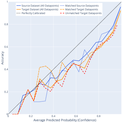
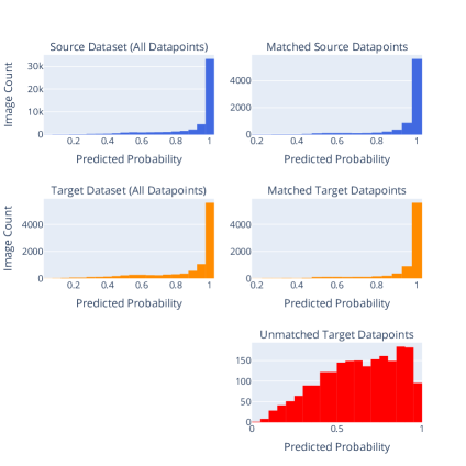
Figure 5: The plots of characteristics of a pre-trained ResNext101 model [27] when evaluated on various subsets of the ImageNetV1 and ImageNetV2 datasets, as generated by our proposed evaluation protocol: (a) accuracy versus confidence and (b) density plots for the predicted probabilities.

5 Conclusions and Future Work

DNN classification models are complex and are equally trained on complex data. By using simplistic evaluation protocols that do not fully account for the rich information generated by these classification models, incomplete or incorrect conclusions about their performance could be drawn. This is even more crucial when comparing the performance of models on multiple similar-but-non-identical datasets. For such evaluation scenarios, using accuracy alone to directly compare the performance of a model over multiple datasets (on all the datapoints available) might not be adequate since these datasets could have valid differences. If the predictions of a model on multiple datasets are consistent, it is fair to expect the performance of the model on matched subsets of these datasets to be similar. We believe that the consistent behaviour of a model in different environments is a desirable property.

In this paper, we introduced a principled evaluation protocol that is suitable for the comparison of the performance of models on multiple similar-but-non-identical test datasets. Specifically, by leveraging the proposed evaluation protocol to generate accuracy values for matched subsets from pairs of test datasets, we were able to perform an in-depth investigation of $278$ CIFAR-10 and $286$ ImageNet models on the original ImageNet and CIFAR-10 datasets, as well as their replication datasets. Our experimental results demonstrate that the deterioration in accuracy may not be as large as was reported by prior research efforts, if the uncertainty-related information generated by DNN models is utilized. While it is encouraging that softmax probabilities contain uncertainty-related information and that these probabilities can serve as a baseline for the uncertainty of a model, it may be valuable to further utilize the proposed evaluation protocol together with alternative uncertainty estimation techniques. Furthermore, it would be of interest to evaluate the consistency of the accuracy metric with respect to the uncertainty estimates in settings with identifiable covariate shift. Finally, we hope that the results presented in this paper will lend support to other research efforts that emphasize the importance of leveraging model uncertainty for evaluation purposes.

Appendix A Appendix

A.1 Description of the Datasets

Table 1: Description of the dataset partitions for CIFAR-10 and its replication datasets.

Name	Default Available	Partition	Total
	Partitions	Used	Images
CIFAR-10	Train, Test	Test	$10,000$
CIFAR-10.1	Test	Test	$2,000$
CIFAR-10.2	Test	Test	$10,000$
CINIC-10	Train, Validation, Test	Test	$90,000$

A.2 Description of the Trained Models

Table 2: Description of the characteristics of the trained models for CIFAR-10.

Network Architectures	VGG [30], ResNet [28], DenseNet [31], ResNeXt [32], ResNet_Preact [33], Shake_Shake [34] PyramidNet [35], SENet [36]
Loss Functions	Focal Loss [37], Brier Loss [38], Maximum Mean Calibration Error (MMCE) Loss [14], Label Smoothing Loss [39]
Data Augmentations (Basic)	Random Cropping, Horizontal Flipping
Data Augmentations (Advanced)	CutMix [40], MixUp [41], RICAP [42]

Table 3: Network architectures and names of the models pre-trained on ImageNet.

Network Architectures

VGG [30], DenseNet [31], ResNet [28], ResNeXt [32], Inception-ResNet [43], EfficientNet [44], DPN [45], SEResNet [46], HRNet [47], DeiT [48] PNasNet [49], Visformer [50], Vision Transformers (ViT) [51]

Pre-trained Models [24]

densenet161, deit_tiny_distilled_patch16_224, dpn68b, efficientnet_b2, dpn92, gluon_resnet50_v1d, gluon_seresnext50_32x4d, gluon_seresnext101_32x4d, hrnet_w18_small_v2, ig_resnext101_32x8d, ig_resnext101_32x16d, legacy_seresnet50, ig_resnext101_32x32d, ig_resnext101_32x48d, inception_resnet_v2, pnasnet5large, resnet18, seresnext50_32x4d, tf_efficientnet_b5, tf_efficientnet_l2_ns, vgg13, visformer_small, vit_base_patch16_224, vit_tiny_patch16_384

A.3 Matching by Predicted Probabilities Only

Algorithm 2 Strategy for matching two datasets based on the predicted model probabilities only.

procedure MatchPredictions($f_{\bm{\theta}}$, $\mathcal{D_{\mathrm{src}}}$, $\mathcal{D_{\mathrm{tgt}}}$, $\epsilon$)

     $\mathcal{P}_{\mathrm{src}}\leftarrow\textsc{Predict}(f_{\bm{\theta}},\mathcal{D_{\mathrm{src}}})$

     $\mathcal{P}_{\mathrm{tgt}}\leftarrow\textsc{Predict}(f_{\bm{\theta}},\mathcal{D_{\mathrm{tgt}}})$

     Initialize 3 empty arrays:

     $\mathcal{P}_{\mathrm{src\_matched}}$ = [ ]

     $\mathcal{P}_{\mathrm{tgt\_matched}}$ = [ ]

     $\mathcal{P}_{\mathrm{tgt\_unmatched}}$ = [ ]

     $N\leftarrow\textsc{Length}(\mathcal{P}_{\mathrm{tgt}})$

     for $i\leftarrow 1,N$ do

         $y_{t},\hat{y}_{t},\hat{p}_{t}\leftarrow\mathcal{P}_{\mathrm{tgt}}[i]$

         $y_{s},\hat{y}_{s},\hat{p}_{s},is\_match\leftarrow\textsc{Match}(y_{t},\hat{y}_{t},\hat{p}_{t},\mathcal{P}_{\mathrm{src}},\epsilon)$

         if $is\_match$ then

              $\mathcal{P}_{\mathrm{src\_matched}}.append((y_{s},\hat{y}_{s},\hat{p}_{s}))$

              $\mathcal{P}_{\mathrm{tgt\_matched}}.append((y_{t},\hat{y}_{t},\hat{p}_{t}))$

         else

              $\mathcal{P}_{\mathrm{tgt\_unmatched}}.append((y_{t},\hat{y}_{t},\hat{p}_{t}))$

         end if

     end forreturn $\mathcal{P}_{\mathrm{src\_matched}},\mathcal{P}_{\mathrm{tgt\_matched}},\mathcal{P}_{\mathrm{tgt\_unmatched}}$

end procedure

function Match($y_{t},\hat{y}_{t},\hat{p}_{t},\mathcal{P}_{\mathrm{src}},\epsilon$)

     Initialize an empty $\mathcal{P}_{\mathrm{matched}}$ = [ ]

     for all $(y,\hat{y},\hat{p})\in\mathcal{P}_{\mathrm{src}}$ do

         if $\hat{p}_{t}\in[\hat{p}-\epsilon,\hat{p}+\epsilon]$ then

              $\mathcal{P}_{\mathrm{matched}}.append((y,\hat{y},\hat{p}))$

         end if

     end for

     if |$\mathcal{P}_{\mathrm{matched}}$| > 0 then

         $(y_{s},\hat{y}_{s},\hat{p}_{s})\leftarrow\textsc{RandomSelect}(\mathcal{P}_{\mathrm{matched}})$

         $\mathcal{P}_{\mathrm{src}}.remove((y,\hat{y},\hat{p}))$

         return $(y_{s},\hat{y}_{s},\hat{p}_{s},is\_match)$

     else

         return $(0,0,0,False)$

     end if

end function
$\triangleright$ The Predict(.) function returns the predictions of a model in an array that consists of tuples $(y,\hat{y},\hat{p})$, where $y$, $\hat{y}$, and $\hat{p}$ denote the ground truth label, the predicted label, and the predicted probability, respectively.
$\triangleright$ The RandomSelect(.) function returns a randomly selected tuple $(y,\hat{y},\hat{p})$ from the array that contains the input tuples.
$\triangleright$ The $\mathcal{P}_{\mathrm{src}}.remove((y,\hat{y},\hat{p}))$ in RandomSelect(.) accounts for random selection without replacement.

A.4 Results for Matching by Predicted Probabilities Only

[] [][] [][] []

[] []

A.5 Additional Results for the Accuracy versus Confidence Curves

[] []

References

- [1] Benjamin Recht, Rebecca Roelofs, Ludwig Schmidt, and Vaishaal Shankar. Do ImageNet Classifiers Generalize to ImageNet? In Kamalika Chaudhuri and Ruslan Salakhutdinov, editors, Proceedings of the 36th International Conference on Machine Learning, volume 97 of Proceedings of Machine Learning Research, pages 5389–5400. PMLR, 09–15 Jun 2019.
- [2] Shangyun Lu, Bradley Nott, Aaron Olson, Alberto Todeschini, Puya Vahabi, Carmon Yair, and Ludwig Schmidt. Harder or Different? A Closer Look at Distribution Shift in Dataset Reproduction. In Uncertainty and Robustness in Deep Learning Workshop (UDL), ICML, 2020.
- [3] Alex Krizhevsky, Vinod Nair, and Geoffrey Hinton. CIFAR-10 (Canadian Institute for Advanced Research). 2009.
- [4] Jia Deng, Wei Dong, Richard Socher, Li-Jia Li, Kai Li, and Li Fei-Fei. Imagenet: A Large-scale Hierarchical Image Database. In 2009 IEEE conference on computer vision and pattern recognition, pages 248–255. Ieee, 2009.
- [5] Antonio Torralba and Alexei A. Efros. Unbiased Look at Dataset Bias. In CVPR. IEEE Computer Society, 2011.
- [6] Curtis G. Northcutt, Anish Athalye, and Jonas Mueller. Pervasive Label Errors in Test Sets Destabilize Machine Learning Benchmarks. In Thirty-fifth Conference on Neural Information Processing Systems Datasets and Benchmarks Track (Round 1), 2021.
- [7] Logan Engstrom, Andrew Ilyas, Shibani Santurkar, Dimitris Tsipras, Jacob Steinhardt, and Aleksander Madry. Identifying statistical bias in dataset replication. In Proceedings of the 37th International Conference on Machine Learning, ICML 2020, 13-18 July 2020, Virtual Event, volume 119 of Proceedings of Machine Learning Research, pages 2922–2932. PMLR, 2020.
- [8] Chuan Guo, Geoff Pleiss, Yu Sun, and Kilian Q. Weinberger. On Calibration of Modern Neural Networks. In Doina Precup and Yee Whye Teh, editors, Proceedings of the 34th International Conference on Machine Learning, volume 70 of Proceedings of Machine Learning Research, pages 1321–1330. PMLR, 06–11 Aug 2017.
- [9] Matthias Hein, Maksym Andriushchenko, and Julian Bitterwolf. Why ReLU Networks Yield High-Confidence Predictions Far Away From the Training Data and How to Mitigate the Problem. In IEEE Conference on Computer Vision and Pattern Recognition, CVPR 2019, Long Beach, CA, USA, June 16-20, 2019, pages 41–50. Computer Vision Foundation / IEEE, 2019.
- [10] Dan Hendrycks and Kevin Gimpel. A Baseline for Detecting Misclassified and Out-of-Distribution Examples in Neural Networks. In 5th International Conference on Learning Representations, ICLR 2017, Toulon, France, April 24-26, 2017, Conference Track Proceedings. OpenReview.net, 2017.
- [11] Jishnu Mukhoti, Viveka Kulharia, Amartya Sanyal, Stuart Golodetz, Philip Torr, and Puneet Dokania. Calibrating Deep Neural Networks Using Focal Loss. Advances in Neural Information Processing Systems, 33:15288–15299, 2020.
- [12] Tim Pearce, Alexandra Brintrup, and Jun Zhu. Understanding Softmax Confidence and Uncertainty. CoRR, abs/2106.04972, 2021.
- [13] Ian J. Goodfellow, Yoshua Bengio, and Aaron Courville. Deep Learning. MIT Press, Cambridge, MA, USA, 2016. http://www.deeplearningbook.org.
- [14] Aviral Kumar, Sunita Sarawagi, and Ujjwal Jain. Trainable Calibration Measures for Neural Networks from Kernel Mean Embeddings. In Jennifer Dy and Andreas Krause, editors, Proceedings of the 35th International Conference on Machine Learning, volume 80 of Proceedings of Machine Learning Research, pages 2805–2814. PMLR, 10–15 Jul 2018.
- [15] Wesley J. Maddox, Pavel Izmailov, Timur Garipov, Dmitry P. Vetrov, and Andrew Gordon Wilson. A Simple Baseline for Bayesian Uncertainty in Deep Learning. In Hanna M. Wallach, Hugo Larochelle, Alina Beygelzimer, Florence d’Alché-Buc, Emily B. Fox, and Roman Garnett, editors, Advances in Neural Information Processing Systems 32: Annual Conference on Neural Information Processing Systems 2019, NeurIPS 2019, December 8-14, 2019, Vancouver, BC, Canada, pages 13132–13143, 2019.
- [16] Jishnu Mukhoti, Andreas Kirsch, Joost van Amersfoort, Philip H. S. Torr, and Yarin Gal. Deterministic Neural Networks with Appropriate Inductive Biases Capture Epistemic and Aleatoric Uncertainty. CoRR, abs/2102.11582, 2021.
- [17] Ranganath Krishnan and Omesh Tickoo. Improving model calibration with accuracy versus uncertainty optimization. In H. Larochelle, M. Ranzato, R. Hadsell, M. F. Balcan, and H. Lin, editors, Advances in Neural Information Processing Systems, volume 33, pages 18237–18248. Curran Associates, Inc., 2020.
- [18] M. P. Naeini, F. C. Gregory, and M. Hauskrecht. Obtaining Well Calibrated Probabilities Using Bayesian Binning. Proceedings of the … AAAI Conference on Artificial Intelligence. AAAI Conference on Artificial Intelligence, 2015:2901–2907, 2015.
- [19] Jeremy Nixon, Mike Dusenberry, Linchuan Zhang, Ghassen Jerfel, and Dustin Tran. Measuring Calibration in Deep Learning, 2019. cite arxiv:1904.01685.
- [20] Yukun Ding, Jinglan Liu, Jinjun Xiong, and Yiyu Shi. Evaluation of Neural Network Uncertainty Estimation with Application to Resource-Constrained Platforms. CoRR, abs/1903.02050, 2019.
- [21] John T. Chu. Optimal Decision Functions for Computer Character Recognition. J. ACM, 12(2):213–226, 1965.
- [22] Corinna Cortes, Giulia DeSalvo, and Mehryar Mohri. Learning with Rejection. In Ronald Ortner, Hans Ulrich Simon, and Sandra Zilles, editors, Algorithmic Learning Theory - 27th International Conference, ALT 2016, Bari, Italy, October 19-21, 2016, Proceedings, volume 9925 of Lecture Notes in Computer Science, pages 67–82, 2016.
- [23] Luke N. Darlow, Elliot J. Crowley, Antreas Antoniou, and Amos J. Storkey. CINIC-10 is not imagenet or CIFAR-10. CoRR, abs/1810.03505, 2018.
- [24] Ross Wightman. Pytorch image models. https://github.com/rwightman/pytorch-image-models, 2019.
- [25] John P Miller, Rohan Taori, Aditi Raghunathan, Shiori Sagawa, Pang Wei Koh, Vaishaal Shankar, Percy Liang, Yair Carmon, and Ludwig Schmidt. Accuracy on the Line: on the Strong Correlation Between Out-of-Distribution and In-Distribution Generalization. In Marina Meila and Tong Zhang, editors, Proceedings of the 38th International Conference on Machine Learning, volume 139 of Proceedings of Machine Learning Research, pages 7721–7735. PMLR, 18–24 Jul 2021.
- [26] Alexandru Niculescu-Mizil and Rich Caruana. Predicting good Probabilities with Supervised Learning. In Luc De Raedt and Stefan Wrobel, editors, Machine Learning, Proceedings of the Twenty-Second International Conference (ICML 2005), Bonn, Germany, August 7-11, 2005, volume 119 of ACM International Conference Proceeding Series, pages 625–632. ACM, 2005.
- [27] Dhruv Mahajan, Ross B. Girshick, Vignesh Ramanathan, Kaiming He, Manohar Paluri, Yixuan Li, Ashwin Bharambe, and Laurens van der Maaten. Exploring the limits of weakly supervised pretraining. In Vittorio Ferrari, Martial Hebert, Cristian Sminchisescu, and Yair Weiss, editors, Computer Vision - ECCV 2018 - 15th European Conference, Munich, Germany, September 8-14, 2018, Proceedings, Part II, volume 11206 of Lecture Notes in Computer Science, pages 185–201. Springer, 2018.
- [28] Kaiming He, Xiangyu Zhang, Shaoqing Ren, and Jian Sun. Deep Residual Learning for Image Recognition. In 2016 IEEE Conference on Computer Vision and Pattern Recognition (CVPR), pages 770–778, 2016.
- [29] I. Zeki Yalniz, Hervé Jégou, Kan Chen, Manohar Paluri, and Dhruv Mahajan. Billion-scale Semi-Supervised Learning for Image Classification. CoRR, abs/1905.00546, 2019.
- [30] Karen Simonyan and Andrew Zisserman. Very Deep Convolutional Networks for Large-Scale Image Recognition. In International Conference on Learning Representations, 2015.
- [31] Gao Huang, Zhuang Liu, Laurens Van Der Maaten, and Kilian Q. Weinberger. Densely Connected Convolutional Networks. In 2017 IEEE Conference on Computer Vision and Pattern Recognition (CVPR), pages 2261–2269, 2017.
- [32] Saining Xie, Ross Girshick, Piotr Dollár, Zhuowen Tu, and Kaiming He. Aggregated Residual Transformations for Deep Neural Networks. In 2017 IEEE Conference on Computer Vision and Pattern Recognition (CVPR), pages 5987–5995, 2017.
- [33] Kaiming He, Xiangyu Zhang, Shaoqing Ren, and Jian Sun. Identity Mappings in Deep Residual Networks. CoRR, abs/1603.05027, 2016.
- [34] Xavier Gastaldi. Shake-Shake regularization. CoRR, abs/1705.07485, 2017.
- [35] Dongyoon Han, Jiwhan Kim, and Junmo Kim. Deep Pyramidal Residual Networks. In 2017 IEEE Conference on Computer Vision and Pattern Recognition (CVPR), pages 6307–6315, 2017.
- [36] Jie Hu, Li Shen, and Gang Sun. Squeeze-and-Excitation Networks. In 2018 IEEE/CVF Conference on Computer Vision and Pattern Recognition, pages 7132–7141, 2018.
- [37] Tsung-Yi Lin, Priya Goyal, Ross B. Girshick, Kaiming He, and Piotr Dollár. Focal Loss for Dense Object Detection. 2017 IEEE International Conference on Computer Vision (ICCV), pages 2999–3007, 2017.
- [38] Glenn W. Brier. Verification of Forecasts Expressed in Terms of Probability. Monthly Weather Review, 1950.
- [39] Rafael Müller, Simon Kornblith, and Geoffrey E Hinton. When does label smoothing help? In H. Wallach, H. Larochelle, A. Beygelzimer, F. d'Alché-Buc, E. Fox, and R. Garnett, editors, Advances in Neural Information Processing Systems, volume 32. Curran Associates, Inc., 2019.
- [40] Sangdoo Yun, Dongyoon Han, Seong Joon Oh, Sanghyuk Chun, Junsuk Choe, and Youngjoon Yoo. CutMix: Regularization Strategy to Train Strong Classifiers with Localizable Features. In International Conference on Computer Vision (ICCV), 2019.
- [41] Hongyi Zhang, Moustapha Cissé, Yann N. Dauphin, and David Lopez-Paz. mixup: Beyond Empirical Risk Minimization. CoRR, abs/1710.09412, 2017.
- [42] Ryo Takahashi, Takashi Matsubara, and Kuniaki Uehara. RICAP: Random Image Cropping and Patching Data Augmentation for Deep CNNs. In Jun Zhu and Ichiro Takeuchi, editors, Proceedings of The 10th Asian Conference on Machine Learning, volume 95 of Proceedings of Machine Learning Research, pages 786–798. PMLR, 14–16 Nov 2018.
- [43] Christian Szegedy, Sergey Ioffe, Vincent Vanhoucke, and Alexander A. Alemi. Inception-v4, Inception-ResNet and the Impact of Residual Connections on Learning. In Satinder P. Singh and Shaul Markovitch, editors, Proceedings of the Thirty-First AAAI Conference on Artificial Intelligence, February 4-9, 2017, San Francisco, California, USA, pages 4278–4284. AAAI Press, 2017.
- [44] Mingxing Tan and Quoc V. Le. EfficientNet: Rethinking Model Scaling for Convolutional Neural Networks. In Kamalika Chaudhuri and Ruslan Salakhutdinov, editors, Proceedings of the 36th International Conference on Machine Learning, ICML 2019, 9-15 June 2019, Long Beach, California, USA, volume 97 of Proceedings of Machine Learning Research, pages 6105–6114. PMLR, 2019.
- [45] Yunpeng Chen, Jianan Li, Huaxin Xiao, Xiaojie Jin, Shuicheng Yan, and Jiashi Feng. Dual Path Networks. In Isabelle Guyon, Ulrike von Luxburg, Samy Bengio, Hanna M. Wallach, Rob Fergus, S. V. N. Vishwanathan, and Roman Garnett, editors, Advances in Neural Information Processing Systems 30: Annual Conference on Neural Information Processing Systems 2017, December 4-9, 2017, Long Beach, CA, USA, pages 4467–4475, 2017.
- [46] Jie Hu, Li Shen, Samuel Albanie, Gang Sun, and Enhua Wu. Squeeze-and-Excitation Networks. IEEE Trans. Pattern Anal. Mach. Intell., 42(8):2011–2023, 2020.
- [47] Guoqing Zhang, Yu Ge, Zhicheng Dong, Hao Wang, Yuhui Zheng, and Shengyong Chen. Deep High-Resolution Representation Learning for Cross-Resolution Person Re-Identification. IEEE Trans. Image Process., 30:8913–8925, 2021.
- [48] Hugo Touvron, Matthieu Cord, Matthijs Douze, Francisco Massa, Alexandre Sablayrolles, and Hervé Jégou. Training Data-efficient Image Transformers & Distillation Through Attention. In Marina Meila and Tong Zhang, editors, Proceedings of the 38th International Conference on Machine Learning, ICML 2021, 18-24 July 2021, Virtual Event, volume 139 of Proceedings of Machine Learning Research, pages 10347–10357. PMLR, 2021.
- [49] Chenxi Liu, Barret Zoph, Jonathon Shlens, Wei Hua, Li-Jia Li, Li Fei-Fei, Alan L. Yuille, Jonathan Huang, and Kevin Murphy. Progressive Neural Architecture Search. CoRR, abs/1712.00559, 2017.
- [50] Zhengsu Chen, Lingxi Xie, Jianwei Niu, Xuefeng Liu, Longhui Wei, and Qi Tian. Visformer: The Vision-friendly Transformer. CoRR, abs/2104.12533, 2021.
- [51] Alexey Dosovitskiy, Lucas Beyer, Alexander Kolesnikov, Dirk Weissenborn, Xiaohua Zhai, Thomas Unterthiner, Mostafa Dehghani, Matthias Minderer, Georg Heigold, Sylvain Gelly, Jakob Uszkoreit, and Neil Houlsby. An image is worth 16x16 words: Transformers for image recognition at scale. In 9th International Conference on Learning Representations, ICLR 2021, Virtual Event, Austria, May 3-7, 2021, 2021.