Positivity and discretization of
Fredholm integral operators

Abstract

We provide sufficient conditions for vector-valued Fredholm integral operators and their commonly used spatial discretizations to be positive in terms of an order relation induced by a corresponding order cone. It turns out that reasonable Nyström methods preserve positivity. Among the projection methods, persistence is obtained for the simplest ones based on polynomial, piecewise linear or specific cubic interpolation (collocation), as well as for piecewise constant basis functions in a Bubnov-Galerkin approach. However, for semi-discretizations using quadratic splines or $\operatorname{sinc}$-collocation we demonstrate that positivity is violated. Our results are illustrated in terms of eigenpairs for Krein-Rutman operators and form the basis of corresponding investigations for nonlinear integral operators.

1 Introduction

Fredholm integral operators canonically arise in numerous applications ranging from a classical fixed-point formulation of linear elliptic boundary value problems [1] to Fréchet derivatives of recent models in theoretical ecology [15, pp. 23ff]. Often their Green’s function resp. kernel is positive. This is understood that such a matrix-valued function preserves an order relation induced by an order cone. For instance, dispersal kernels used in theoretical ecology preserve an order relation in order to capture predator-prey or symbiotic relationships between different species, or differential operators satisfy a maximum principle which transfers to positivity of their inverses via the Green’s function. Moreover, for example [7] provides sufficient conditions that Hammerstein operators can be transformed into an order-preserving form.

Dealing with positive operators has several merits. First, positivity allows an application of the Krein-Rutman theorem [5, p. 226, Thm. 19.2], [24, p. 290, Thm. 7.C] or [14] with profound consequences to the bifurcation behavior of related nonlinear problems. Second, [2] gives results on the distribution of secondary eigenvalues. Finally, criteria for various types of positivity in linear operators are fundamental to obtain corresponding results for nonlinear integral operators of Urysohn or Hammerstein type [17, 18]. Beyond providing sufficient conditions for positivity of Fredholm integral operators, in this paper we also discuss the question whether this property is preserved under discretizations. The latter aspect is crucial in numerical simulations and computations in order to preserve or capture properties of the original problem.

More detailled, the texture of this paper is as follows: After introducing our notation, Sect. 2 provides sufficient conditions on kernels such that the associated Fredholm operators on the continuous or integrable functions are positive over domains of finite measure. In essence these properties carry over from the kernels having values in ${\mathbb{R}}^{d}$ to the integral operators mapping into a space of ${\mathbb{R}}^{d}$-valued functions. Persistence issues under full spatial discretization of Nyström type are tackled in Sect. 3. It suffices to assume positive quadrature weights for the sake of positivity. This property is satisfied for a large class of integration methods [4, 11] and, besides guaranteeing well-posedness and computational stability [9, 10], provides another reason for the use of positive weights in numerical quadrature. This convenient prospect changes in Sect. 4 when addressing semi-discretizations of projection type. Here the situation is more subtle and the class of positivity-preserving schemes appears to be rather small. Among the collocation methods we indeed observe that polynomial and piecewise linear collocation preserves positivity, while popular other methods (e.g. quadratic splines, $\operatorname{sinc}$ methods) do not. Among the Bubnov-Galerkin methods, at least piecewise constant approximation works. Nevertheless, based on positivity-preserving interpolation methods [20, 21, 23] it appears to be possible to construct projection operators, which are positive at least on subsets of the state space. Pointing towards applications, Sect. 5 discusses order-preserving properties of typical dispersal kernels and illustrates our results by means of a failure in the Krein-Rutman theorem when using quadrature schemes having negative weights. Moreover, we compare numerical errors for various projection methods when approximating the dominant eigenvalue of a positive operator. For the reader’s convenience, an appendix collects basic results on cones in Banach spaces and positive operators, an explicit formula for the inverse of tridiagonal matrices and lists the quadrature rules in Nyström methods throughout the text.

Notation: We abbreviate ${\mathbb{R}}_{+}:=[0,\infty)$ for the nonnegative reals, $\delta_{ij}\in\left\{0,1\right\}$ is the Kronecker symbol and the Euclidean inner product in ${\mathbb{R}}^{d}$ is given by $\langle\!\!\langle x,y\rangle\!\!\rangle:=\sum_{j=1}^{d}x_{j}y_{j}$ for $x,y\in{\mathbb{R}}^{d}$.

Norms on finite-dimensional spaces are denoted by $\left|\cdot\right|$ and unless otherwise stated we use the Euclidean norm. Given a matrix $T\in{\mathbb{R}}^{d\times d}$ we write $T_{ij}\in{\mathbb{R}}$ for the $j$th element in the $i$th row and $I_{d}\in{\mathbb{R}}^{d\times d}$ is the identity matrix. Throughout, $Y_{+}\subset{\mathbb{R}}^{d}$ denotes an order cone inducing the relations $\leqslant,<$ and $\ll$ (cf. (A.1) and App. A for related terminology); $Y_{+}^{\prime}$ is the dual cone.

On metric spaces $(X,d)$, $U^{\circ}$ denotes the interior, $\overline{U}$ the closure of a set $U\subseteq X$, and $B_{r}(x):=\left\{y\in X:\,d(y,x)<r\right\}$ the open ball of radius $r>0$ and $x\in X$.

With Banach spaces $X,Y$ we write $L(X,Y)$ for the linear space of bounded linear maps $T:X\to Y$, $L(X):=L(X,X)$ and $X^{\prime}:=L(X,{\mathbb{R}})$ for the dual space, as well as $N(T):=T^{-1}(\left\{0\right\})$ for the kernel of $T$.

2 Fredholm integral operators

This section provides sufficient conditions for Fredholm (integral) operators

$${\mathscr{K}}u:=\int_{\Omega}K(\cdot,y)u(y)\,{\mathrm{d}}\mu(y) F$$ ()

to preserve order relations. In essence, we demonstrate that related positivity properties of the kernels $K:\Omega^{2}\to L({\mathbb{R}}^{d})$ carry over to integral operators ${\mathscr{K}}$.

For this purpose and referring to later applications it is ambient to work with an abstract measure-theoretical integral in ($F$). Thereto, assume $(\Omega,{\mathfrak{A}},\mu)$ is a measure space satisfying $\mu(\Omega)<\infty$. The resulting abstract $\mu$-integral of a $\mu$-measurable function $u:\Omega\to{\mathbb{R}}^{d}$ is denoted by $\int_{\Omega}u(y)\,{\mathrm{d}}\mu(y)$ and satisfies

$$\langle\!\!\langle\int_{\Omega}u(y)\,{\mathrm{d}}\mu(y),y^{\prime}\rangle\!\!\rangle=\int_{\Omega}\langle\!\!\langle u(y),y^{\prime}\rangle\!\!\rangle\,{\mathrm{d}}\mu(y)\quad\text{for all }y^{\prime}\in{\mathbb{R}}^{d}.$$ (2.1)

A relevant case in applications [15] is the $\kappa$-dimensional Lebesgue measure $\mu=\lambda_{\kappa}$ on $\Omega\subset{\mathbb{R}}^{\kappa}$ yielding the Lebesgue integral $\int_{\Omega}u(y)\,{\mathrm{d}}y:=\int_{\Omega}u(y)\,{\mathrm{d}}\lambda_{\kappa}(y)$ for functions $u:\Omega\to{\mathbb{R}}^{d}$. Moreover, numerical numerical analysis relies on

Remark 2.1 (quadrature methods as abstract integrals)

Let $\Omega^{\prime}\subset{\mathbb{R}}^{\kappa}$ be countable and $\eta\in\Omega^{\prime}$ with associated reals $w_{\eta}\geq 0$. Then $\mu(\Omega^{\prime}):=\sum_{\eta\in\Omega^{\prime}}w_{\eta}$ is a measure on the family of countable subsets of ${\mathbb{R}}^{\kappa}$. Note that $\sum_{\eta\in\Omega^{\prime}}w_{\eta}<\infty$ gives $\mu(\Omega^{\prime})<\infty$ and the $\mu$-integral is $\int_{\Omega^{\prime}}u(y)\,{\mathrm{d}}\mu(y)=\sum_{\eta\in\Omega^{\prime}}w_{\eta}u(\eta)$. This setting includes the case, where $\Omega^{\prime}$ is a finite set $\Omega_{n}=\left\{\eta_{j}:\,0\leqslant j\leqslant q_{n}\right\}$ of nodes $\eta_{j}$ with associated weights $w_{\eta}=w_{j}$ of a numerical quadrature rule [3, 9], where $(q_{n})_{n\in{\mathbb{N}}}$ is a strictly increasing sequence of positive integers. Here,

$$\mu(\Omega_{n}) =\sum_{j=0}^{q_{n}}w_{j}, \int_{\Omega_{n}}u(y)\,{\mathrm{d}}\mu(y) =\sum_{j=0}^{q_{n}}w_{j}u(\eta_{j})$$

for all functions $u:\Omega_{n}\to{\mathbb{R}}^{d}$. Concrete examples are listed in App. C.

2.1 Fredholm operators on $C(\Omega)^{d}$

In this subsection, we restrict to measure spaces $(\Omega,{\mathfrak{A}},\mu)$ with a compact metric space $\Omega$, a $\sigma$-algebra ${\mathfrak{A}}$ (containing the Borel sets) and a finite measure $\mu$, i.e. $\mu(\Omega)<\infty$.

The set $C(\Omega)^{d}$ of continuous functions $u:\Omega\to{\mathbb{R}}^{d}$ is a real Banach space when equipped with the maximum norm $\left\|u\right\|_{\infty}:=\max_{x\in\Omega}\left|u(x)\right|$. Moreover,

$$C(\Omega)^{d}_{+}:=\left\{u\in C(\Omega)^{d}:\,u(x)\in Y_{+}\text{ for all }x\in\Omega\right\}$$

abbreviates the set of continuous functions having values in a cone $Y_{+}\subset{\mathbb{R}}^{d}$.

Lemma 2.2

The set $C(\Omega)^{d}_{+}$ is a cone. If $Y_{+}$ is solid, then $C(\Omega)^{d}_{+}$ is solid and total.

[Proof.] The closedness and convexity of $Y_{+}$ extend to $C(\Omega)^{d}_{+}$ and a pointwise consideration yields ${\mathbb{R}}_{+}C(\Omega)^{d}_{+}\subseteq C(\Omega)^{d}_{+}$ and $C(\Omega)^{d}_{+}\cap(-C(\Omega)^{d}_{+})=\left\{0\right\}$. Thus, $C(\Omega)^{d}_{+}$ is a cone. If $Y_{+}\subset{\mathbb{R}}^{d}$ is solid, then there exist $y_{0}\in Y_{+}$ and $\varepsilon>0$ so that $B_{\varepsilon}(y_{0})\subset Y_{+}$. Hence, $u_{0}(x):\equiv y_{0}$ on $\Omega$ is an interior point of $C(\Omega)^{d}_{+}$ and $(C(\Omega)^{d}_{+})^{\circ}\neq\emptyset$ follows. ∎

Having identified $C(\Omega)^{d}_{+}$ as (solid) cone, we introduce the relations (cf. (A.1))

$$u\preceq\bar{u}\quad :\Leftrightarrow\quad\bar{u}-u\in C(\Omega)^{d}_{+},$$

$$u\prec\bar{u}\quad :\Leftrightarrow\quad\bar{u}-u\in C(\Omega)^{d}_{+}\setminus\left\{0\right\},$$

$$u\prec\!\!\!\prec\bar{u}\quad :\Leftrightarrow\quad\bar{u}-u\in(C(\Omega)^{d}_{+})^{\circ}\quad\text{for all }u,\bar{u}\in C(\Omega)^{d},$$

allowing the subsequent characterization:

Lemma 2.3

The following holds for $u,\bar{u}\in C(\Omega)^{d}$:

1. $u\preceq\bar{u}\Leftrightarrow u(x)\leqslant\bar{u}(x)$ for all $x\in\Omega$ $\Leftrightarrow\langle\!\!\langle u(x),y^{\prime}\rangle\!\!\rangle\leqslant\langle\!\!\langle\bar{u}(x),y^{\prime}\rangle\!\!\rangle$ for all $x\in\Omega$ and $y^{\prime}\in Y_{+}^{\prime}$.

2. $u\prec\bar{u}\Leftrightarrow u(x)\leqslant\bar{u}(x)$ for all $x\in\Omega$ and $u(x_{0})<\bar{u}(x_{0})$ for some $x_{0}\in\Omega$.

3. If $Y_{+}$ is solid, then $u\prec\!\!\!\prec\bar{u}\Leftrightarrow u(x)\ll\bar{u}(x)$ for all $x\in\Omega$ $\Leftrightarrow\langle\!\!\langle u(x),y^{\prime}\rangle\!\!\rangle<\langle\!\!\langle\bar{u}(x),y^{\prime}\rangle\!\!\rangle$ for all $x\in\Omega$, $y^{\prime}\in Y_{+}^{\prime}\setminus\left\{0\right\}$.

[Proof.] (a) follows immediately by definition and from Lemma A.1(a).
(b) results from the definition.
(c) Due to linearity it suffices to establish the claim for the pair $(0,u)$ rather than the functions $(u,\bar{u})$. We have to show two directions:
$(\Leftarrow)$ Assume that $0<\langle\!\!\langle u(x),y^{\prime}\rangle\!\!\rangle$ for all $x\in\Omega$, $y^{\prime}\in Y_{+}^{\prime}\setminus\left\{0\right\}$ holds. Therefore, Lemma A.1(b) ensures that for any $x\in\Omega$ there exists an $\varepsilon_{x}>0$ guaranteeing the inclusion $B_{\varepsilon_{x}}(u(x))\subset Y_{+}$. We prove that

$$\exists\varepsilon>0:\forall x\in\Omega:\,B_{\varepsilon}(u(x))\subset Y_{+}.$$ (2.2)

Assuming the contrary there exist sequences $(x_{n})_{n\in{\mathbb{N}}}$ in $\Omega$ and $(z_{n})_{n\in{\mathbb{N}}}$ in ${\mathbb{R}}^{d}$ with

$$\left|z_{n}-u(x_{n}))\right|\leqslant\tfrac{1}{n},\quad z_{n}\notin Y_{+}\quad\text{for all }n\in{\mathbb{N}}.$$ (2.3)

From compactness of $\Omega$ and continuity of $u$ there exists a subsequence $(x_{k_{n}})_{n\in{\mathbb{N}}}$ with limit $x^{\ast}\in\Omega$ such that $\lim_{n\to\infty}z_{k_{n}}=u(x^{\ast})$ is satisfied. Consequently, $z_{k_{n}}\in B_{\varepsilon_{x^{\ast}}}(u(x^{\ast}))\subset Y_{+}$ holds for sufficiently large $n\in{\mathbb{N}}$, contradicting (2.3). Hence, (2.2) holds and implies that $B_{\varepsilon}(u)\subset C(\Omega)^{d}_{+}$ and $0\prec\!\!\!\prec u$.
$(\Rightarrow)$ For $0\prec\!\!\!\prec u$ there exists an $\varepsilon>0$ so that $v(x)\in Y_{+}$ for all $v\in B_{\varepsilon}(u)$ and $x\in\Omega$. Let $x\in\Omega$ and $z_{0}\in B_{\varepsilon}(u(x))\subseteq{\mathbb{R}}^{d}$. If $\bar{v}(\xi):=u(\xi)+z_{0}-u(x)$, $\xi\in\Omega$, then $\bar{v}\in B_{\varepsilon}(u)$ and thus $\bar{v}(\xi)\in Y_{+}$ for all $\xi\in\Omega$. For $\xi=x$ we see that $z_{0}\in Y_{+}$ and $B_{\varepsilon}(u(x))\subset Y_{+}$ for each $x\in\Omega$. Hence, $u(x)\in Y^{\circ}_{+}$ for all $x\in\Omega$. From Lemma A.1(b) we have $0<\langle\!\!\langle u(x),y^{\prime}\rangle\!\!\rangle$ for all $x\in\Omega$, $y^{\prime}\in Y_{+}^{\prime}\setminus\left\{0\right\}$. ∎

Example 2.4

If a set $\left\{e_{1},\ldots,e_{d}\right\}\subset{\mathbb{R}}^{d}$ is linearly independent, then the linear combinations $Y_{+}=\left\{\sum_{i=1}^{d}\alpha_{i}e_{i}:\,\alpha_{1},\ldots,\alpha_{d}\geq 0\right\}\subset{\mathbb{R}}^{d}$ form a solid, thus total cone with interior $Y_{+}^{\circ}=\bigl{\{}\sum_{i=1}^{d}\alpha_{i}e_{i}:\,\alpha_{1},\ldots,\alpha_{d}>0\bigr{\}}$. With $\left\{e_{1}^{\prime},\ldots,e_{d}^{\prime}\right\}\subset{\mathbb{R}}^{d}$ chosen according to $\langle\!\!\langle e_{i},e_{j}^{\prime}\rangle\!\!\rangle=\delta_{ij}$ for $1\leqslant i,j\leqslant d$, then $Y_{+}^{\prime}=\bigl{\{}\sum_{j=1}^{d}\beta_{j}e_{j}^{\prime}:\,\beta_{1},\ldots,\beta_{d}\geq 0\bigr{\}}\subset{\mathbb{R}}^{d}$ is the dual cone to $Y_{+}$. Given $u,\bar{u}\in C(\Omega)^{d}$ one has:

$$u\preceq\bar{u}\quad\Leftrightarrow \quad\langle\!\!\langle u(x),e_{j}^{\prime}\rangle\!\!\rangle\leqslant\langle\!\!\langle\bar{u}(x),e_{j}^{\prime}\rangle\!\!\rangle\text{ for all }x\in\Omega,\,1\leqslant j\leqslant d,$$

$$u\prec\bar{u}\quad\Leftrightarrow \quad\langle\!\!\langle u(x),e_{j}^{\prime}\rangle\!\!\rangle\leqslant\langle\!\!\langle\bar{u}(x),e_{j}^{\prime}\rangle\!\!\rangle\text{ for all }x\in\Omega,\,1\leqslant j\leqslant d$$

$$\quad\text{and }u(x_{0})<\bar{u}(x_{0})\text{ for some }x_{0}\in\Omega,$$

$$u\prec\!\!\!\prec\bar{u}\quad\Leftrightarrow \quad\langle\!\!\langle u(x),e_{j}^{\prime}\rangle\!\!\rangle<\langle\!\!\langle\bar{u}(x),e_{j}^{\prime}\rangle\!\!\rangle\text{ for all }x\in\Omega,\,1\leqslant j\leqslant d.$$

Example 2.5 (orthants)

Let $Y_{+}$ be an orthant of ${\mathbb{R}}^{d}$ spanned by the linearly independent vectors $e_{i}=\varsigma_{i}(\delta_{ij})_{j=1}^{d}$ with $\varsigma_{i}=\pm 1$. For $e_{j}^{\prime}:=\varsigma_{j}(\delta_{ij})_{i=1}^{d}$ one obtains characterizations based on the component functions

$$u\preceq\bar{u}\quad\Leftrightarrow \quad\varsigma_{i}u_{i}(x)\leqslant\varsigma_{i}\bar{u}_{i}(x)\quad\text{for all }x\in\Omega,\,1\leqslant i\leqslant d,$$

$$u\prec\bar{u}\quad\Leftrightarrow \quad\varsigma_{i}u_{i}(x)\leqslant\varsigma_{i}\bar{u}_{i}(x)\quad\text{for all }x\in\Omega,\,1\leqslant i\leqslant d\text{ and there}$$

$$\quad\text{exist }x_{0}\in\Omega,1\leqslant i_{0}\leqslant d\text{ with }u_{i_{0}}(x_{0})\neq\bar{u}_{i_{0}}(x_{0}),$$

$$u\prec\!\!\!\prec\bar{u}\quad\Leftrightarrow \quad\varsigma_{i}u_{i}(x)<\varsigma_{i}\bar{u}_{i}(x)\quad\text{for all }x\in\Omega,\,1\leqslant i\leqslant d.$$

A convenient setting for linear integral operators provides the following

Hypothesis 2.6

Assume that $K:\Omega\times\Omega\to L({\mathbb{R}}^{d})$ fulfills:

• $K(x,\cdot):\Omega\to L({\mathbb{R}}^{d})$ is $\mu$-measurable for all $x\in\Omega$ with

  $$\sup_{x\in\Omega}\int_{\Omega}\left|K(x,y)\right|\,{\mathrm{d}}\mu(y)<\infty$$

  and $\lim_{x\to x_{0}}\int_{\Omega}\left|K(x,y)-K(x_{0},y)\right|\,{\mathrm{d}}\mu(y)=0$ for all $x_{0}\in\Omega$.

These assumptions yield that Fredholm operators ${\mathscr{K}}$ given in ($F$) readily fulfill the inclusion ${\mathscr{K}}\in L(C(\Omega)^{d})$ (see [16, p. 167, Prop. 3.4]). In case the limit relation in $(L)$ holds uniformly in $x_{0}\in\Omega$, then ${\mathscr{K}}$ is even compact; however this is not immediately relevant for our further analysis.

Theorem 2.7 (positivity of ${\mathscr{K}}$ on $C(\Omega)^{d}$)

Let Hypothesis $(L)$ hold. If a kernel $K(x,y)\in L({\mathbb{R}}^{d})$ is $Y_{+}$-positive for all $x\in\Omega$ and $\mu$-a.a. $y\in\Omega$, then a Fredholm operator ${\mathscr{K}}\in L(C(\Omega)^{d})$ is $C(\Omega)^{d}_{+}$-positive. These assumptions additionally yield:

1. If nonempty, open subsets of $\Omega$ have positive measure, there exists a $\bar{x}\in\Omega$ so that $K(\bar{x},\cdot)$ is continuous on $\Omega$ and $K(\bar{x},y)$ is $Y_{+}$-injective for $\mu$-a.a. $y\in\Omega$, then ${\mathscr{K}}$ strictly $C(\Omega)^{d}_{+}$-positive.

2. If nonempty, open subsets of $\Omega$ have positive measure, $Y_{+}$ is solid and $K(x,y)$ is strongly $Y_{+}$-positive for all $x\in\Omega$ and $\mu$-a.a. $y\in\Omega$, then ${\mathscr{K}}$ is strongly $C(\Omega)^{d}_{+}$-positive.

3. If $\mu(\Omega)>0$, $Y_{+}$ is solid and $K(x,y)Y_{+}^{\circ}\subseteq Y_{+}^{\circ}$ for all $x\in\Omega$ and $\mu$-a.a. $y\in\Omega$, then ${\mathscr{K}}(C(\Omega)^{d}_{+})^{\circ}\subseteq(C(\Omega)^{d}_{+})^{\circ}$.

[Proof.] Let $x\in\Omega$, $y^{\prime}\in Y_{+}^{\prime}$ and $0\prec u$. By Lemma 2.3(a) the positivity of ${\mathscr{K}}$ is an immediate consequence of

$$\langle\!\!\langle({\mathscr{K}}u)(x),y^{\prime}\rangle\!\!\rangle\stackrel{{\scriptstyle\eqref{noprod}}}{{=}}\int_{\Omega}\langle\!\!\langle K(x,y)u(y),y^{\prime}\rangle\!\!\rangle\,{\mathrm{d}}\mu(y)\geq 0.$$

Thus, for the remaining proof ${\mathscr{K}}$ is positive.
(a) Let $0\prec u$. There exists a $y_{0}\in\Omega$ such that $\max_{x\in\Omega}\left|u(x)\right|=\left|u(y_{0})\right|>0$ and thus $u_{i_{0}}(y_{0})\neq 0$ for some index $i_{0}\in\{1,\ldots,d\}$. First, if $u_{i_{0}}(y_{0})>0$, then $\Omega_{0}:=\{y\in\Omega:u_{i_{0}}(y)>\tfrac{1}{2}u_{i_{0}}(y_{0})\}=u_{i_{0}}^{-1}((\tfrac{1}{2}u_{i_{0}}(y_{0}),\infty))\neq\emptyset$ and the continuity of $u_{i_{0}}$ yields that $\Omega_{0}$ is open; thus, $\mu(\Omega_{0})>0$ by assumption. Thanks to $Y_{+}$-injectivity, $K(\bar{x},y)u(y)\in Y_{+}\setminus\{0\}$ holds for $\mu$-a.a. $y\in\Omega_{0}$ and Lemma A.1(a) ensures that there exists a functional $y_{y}^{\prime}\in Y_{+}^{\prime}\setminus\{0\}$ satisfying $\langle\!\!\langle K(\bar{x},y)u(y),y_{y}^{\prime}\rangle\!\!\rangle>0$. Due to the continuity of $K(\bar{x},\cdot)$, for $\mu$-a.a. $y\in\Omega_{0}$ there exists $\varepsilon_{y}>0$ such that $\langle\!\!\langle K(\bar{x},\eta)u(\eta),y_{y}^{\prime}\rangle\!\!\rangle>0\quad\text{for}\ \eta\in B_{\varepsilon_{y}}(y).$ Since $\{B_{\varepsilon_{y}}(y):\,\mu\textrm{-a.a.}\ y\in\Omega_{0}\}$ is an open cover of the compact closure $\overline{\Omega_{1}}$, where $\Omega_{1}$ is an open set and $\overline{\Omega_{1}}\subset\Omega_{0}$ the Borel-Lebesgue Theorem yields a finite subcover $\{B_{\varepsilon_{i}}(y_{i}):\,1\leqslant i\leqslant n\}$ of $\overline{\Omega_{1}}$. Moreover $\mu(\Omega_{1})>0$. If we define $\tilde{y}^{\prime}:=\sum^{n}_{i=1}y^{\prime}_{y_{i}}\in Y_{+}^{\prime}\neq 0$, then $\langle\!\!\langle K(\bar{x},y)u(y),\tilde{y}^{\prime}\rangle\!\!\rangle>0$ for $\mu$-a.a. $y\in\Omega_{1}$ and

$$\langle\!\!\langle({\mathscr{K}}u)(\bar{x}),\tilde{y}^{\prime}\rangle\!\!\rangle \stackrel{{\scriptstyle\eqref{nofred}}}{{=}}\langle\!\!\langle\int_{\Omega}K(\bar{x},y)u(y)\,{\mathrm{d}}\mu(y),\tilde{y}^{\prime}\rangle\!\!\rangle\geq\int_{\Omega_{1}}\langle\!\!\langle K(\bar{x},y)u(y),\tilde{y}^{\prime}\rangle\!\!\rangle\,{\mathrm{d}}\mu(y)>0$$

holds. This implies that $({\mathscr{K}}u)(\bar{x})\neq 0$ and therefore ${\mathscr{K}}u\neq 0$ holds. Second, in the dual case $u_{i_{0}}(y_{0})<0$ we use the open set $\{y\in\Omega:\,u_{i_{0}}(y)<\tfrac{1}{2}u_{i_{0}}(y_{0})\}$ instead of $\Omega_{0}$ and again obtain ${\mathscr{K}}u\neq 0$. In conclusion, ${\mathscr{K}}$ is strictly positive.
(b) Let $0\prec u$, $y^{\prime}\in Y_{+}^{\prime}\setminus\left\{0\right\}$, $x\in\Omega$. Note that $\Omega_{0}=\{y\in\Omega:u(y)\neq 0\}$ is open subset of $\Omega$ and $\mu(\Omega_{0})>0$. Since $K(x,y)$ is strongly positive for $\mu$-a.a. $y\in\Omega_{0}$, we get $0\ll K(x,y)u(y)$ and hence Lemma A.1(b) implies $0<\langle\!\!\langle K(x,y)u(y),y^{\prime}\rangle\!\!\rangle=:\phi(y)$ for $\mu$-a.a. $y\in\Omega_{0}$. Now at least one of the preimages $\Omega_{l}:=\phi^{-1}((\tfrac{1}{l},\infty))$, $l\in{\mathbb{N}}$, has positive measure, since $\Omega_{0}=\bigcup_{l\in{\mathbb{N}}}\Omega_{l}$ is of positive measure. In case $\mu(\Omega_{l})>0$ we obtain $0<\frac{\mu(\Omega_{l})}{l}\leqslant\int_{\Omega_{l}}\phi(y)\,{\mathrm{d}}\mu(y)\leqslant\int_{\Omega_{0}}\phi(y)\,{\mathrm{d}}\mu(y)$ and consequently

$$\langle\!\!\langle({\mathscr{K}}u)(x),y^{\prime}\rangle\!\!\rangle\stackrel{{\scriptstyle\eqref{nofred}}}{{=}}\int_{\Omega}\phi(y)\,{\mathrm{d}}\mu(y)\geq\int_{\Omega_{0}}\phi(y)\,{\mathrm{d}}\mu(y)\geq\int_{\Omega_{l}}\phi(y)\,{\mathrm{d}}\mu(y)>0.$$

Because $y\in Y_{+}^{\prime}\setminus\left\{0\right\}$ and $x\in\Omega$ were arbitrary, Lemma A.1(b) readily implies $0\ll({\mathscr{K}}u)(x)$ for any $x\in\Omega$ and therefore ${\mathscr{K}}$ is strongly $C(\Omega)^{d}_{+}$-positive by Lemma 2.3(c).
(c) Let $u\in(C(\Omega)^{d}_{+})^{\circ}$. Then Lemma 2.3(c) yields $0\ll K(x,y)u(y)$ for $\mu$-a.a. $y\in\Omega$ and $x\in\Omega$ and the claim results as in (b). ∎

2.2 Fredholm operators on $L^{p}(\Omega)$

Let $p\in[1,\infty)$ and assume $\mu(\Omega)>0$ throughout. The set $L^{p}(\Omega)^{d}$ of $p$-integrable functions $u:\Omega\to{\mathbb{R}}^{d}$ defines a real Banach space with

$$\left\|u\right\|_{p}:=\left(\int_{\Omega}\left|u(y)\right|^{p}\,{\mathrm{d}}\mu(y)\right)^{1/p}$$

as norm. Let us furthermore write

$$L^{p}(\Omega)_{+}^{d}:=\left\{u\in L^{p}(\Omega)^{d}:\,u(x)\in Y_{+}\text{ for $\mu$-a.a.\ }x\in\Omega\right\}$$

for the set of $p$-integrable functions with values in $Y_{+}$.

Lemma 2.8

The set $L^{p}(\Omega)_{+}^{d}$ is a cone. If $Y_{+}\subseteq{\mathbb{R}}^{d}$ is an orthant, then $L^{p}(\Omega)_{+}^{d}$ is total.

Note that even in case $Y_{+}={\mathbb{R}}_{+}$ the cone $L^{p}(\Omega)_{+}$ is not solid (cf. [1, Ex. 1.11]). Yet, for $Y_{+}={\mathbb{R}}_{+}$ it is reproducing (i.e. $X=Y_{+}-Y_{+}$) and hence total. [Proof.] Closedness and convexity of $Y_{+}$ extend to $L^{p}(\Omega)_{+}^{d}$ and a pointwise consideration yields ${\mathbb{R}}_{+}L^{p}(\Omega)_{+}^{d}\subseteq L^{p}(\Omega)_{+}^{d}$ and $L^{p}(\Omega)_{+}^{d}\cap(-L^{p}(\Omega)_{+}^{d})=\left\{0\right\}$. So, $L^{p}(\Omega)_{+}^{d}$ is a cone. If $Y_{+}\subseteq{\mathbb{R}}^{d}$ is an orthant, then $L^{p}(\Omega)_{+}^{d}$ is reproducing and consequently total. ∎ Having identified the set $L^{p}(\Omega)_{+}^{d}$ as a cone, we introduce the relations (cf. (A.1))

$$u\preceq\bar{u}\quad :\Leftrightarrow\quad\bar{u}-u\in L^{p}(\Omega)_{+}^{d},$$

$$u\prec\bar{u}\quad :\Leftrightarrow\quad\bar{u}-u\in L^{p}(\Omega)_{+}^{d}\setminus\left\{0\right\},$$

allowing the subsequent characterization:

Lemma 2.9

The following holds for $u,\bar{u}\in L^{p}(\Omega)^{d}$:

1. $u\preceq\bar{u}\Leftrightarrow u(x)\leqslant\bar{u}(x)$ for $\mu$-a.a. $x\in\Omega$ $\Leftrightarrow\langle\!\!\langle u(x),y^{\prime}\rangle\!\!\rangle\leqslant\langle\!\!\langle\bar{u}(x),y^{\prime}\rangle\!\!\rangle$ for $\mu$-a.a. $x\in\Omega$ and all $y^{\prime}\in Y_{+}^{\prime}$.

2. $u\prec\bar{u}\Leftrightarrow u(x)\leqslant\bar{u}(x)$ $\mu$-a.a. in $\Omega$ and $\mu(\left\{x\in\Omega:\,u(x)\neq\bar{u}(x)\right\})>0$.

[Proof.] (a) follows immediately from Lemma A.1(a) and by definition.
(b) results from the definition. ∎

Lemma 2.10 (strict monotonicity of the integral)

Let $u,\bar{u}\in L^{p}(\Omega)_{+}^{d}$ w.r.t. an orthant $Y_{+}\subset{\mathbb{R}}^{d}$. If $u\prec\bar{u}$, then $\int_{\Omega}u(y)\,{\mathrm{d}}\mu(y)<\int_{\Omega}\bar{u}(y)\,{\mathrm{d}}\mu(y)$.

[Proof.] It suffices to show that $u\in L^{p}(\Omega)_{+}^{d}\setminus\left\{0\right\}$ implies $\int_{\Omega}u(y)\,{\mathrm{d}}\mu(y)\neq 0$. Let $Y_{+}$ be spanned by the vectors $e_{i}=\varsigma_{i}(\delta_{ij})_{j=1}^{d}$ with $\varsigma_{i}=\pm 1$. Since $u\neq 0$, there exists an index $j$ and a set $\Omega_{0}\subseteq\Omega$ of positive measure with $0<\varsigma_{j}u_{j}(x)$ for $x\in\Omega_{0}$. The sets $\Omega_{l}:=\left\{x\in\Omega_{0}:\,\tfrac{1}{l}\leqslant\varsigma_{j}u_{j}(x)\right\}$ for $l\in{\mathbb{N}}$ fulfill $\Omega_{0}=\bigcup_{l\in{\mathbb{N}}}\Omega_{l}$ and $\Omega_{l}\subseteq\Omega_{l+1}$. Thus, the assumption $\int_{\Omega_{0}}u(y)\,{\mathrm{d}}\mu(y)=0$ leads to $0=\int_{\Omega_{0}}\varsigma_{j}u_{j}(y)\,{\mathrm{d}}\mu(y)\geq\int_{\Omega_{l}}\varsigma_{j}u_{j}(y)\,{\mathrm{d}}\mu(y)=\tfrac{1}{l}\mu(\Omega_{l})$ and hence $\mu(\Omega_{l})=0$ for $l\in{\mathbb{N}}$. Now the continuity of measures implies the contradiction $\mu(\Omega_{0})=0$. ∎

Now we proceed to linear integral operators on the square-integrable functions:

Hypothesis 2.11

Assume that $K:\Omega\times\Omega\to L({\mathbb{R}}^{d})$ fulfills:

• $K:\Omega\times\Omega\to L({\mathbb{R}}^{d})$ is $\mu\otimes\mu$-measurable with

  $$\int_{\Omega}\int_{\Omega}\left|K(x,y)\right|^{2}\,{\mathrm{d}}\mu(y)\,{\mathrm{d}}\mu(x)<\infty.$$

Then the Fredholm operator ${\mathscr{K}}\in L(L^{2}(\Omega)^{d})$ defined via ($F$) is well-defined and also compact (cf. [9, p. 47, Thm. 3.2.7]).

Theorem 2.12 (positivity of ${\mathscr{K}}$ on $L^{2}(\Omega)^{d}$)

Let Hypothesis $(L^{2})$ hold. If a kernel $K(x,y)\in L({\mathbb{R}}^{d})$ is $Y_{+}$-positive for $\mu$-a.a. $x,y\in\Omega$, then a Fredholm operator ${\mathscr{K}}\in L(L^{2}(\Omega))$ is $L^{2}(\Omega)_{+}^{d}$-positive. If moreover, $Y_{+}\subset{\mathbb{R}}^{d}$ is an orthant and $K(x,y)$ is strictly $L^{2}(\Omega)_{+}$-positive for $\mu$-a.a. $x,y\in\Omega$, then ${\mathscr{K}}$ is strictly $L^{2}(\Omega)_{+}^{d}$-positive.

[Proof.] Proving positivity of ${\mathscr{K}}$ is formally identical to the argument in the proof of Thm. 2.7. One merely replaces the reference to Lemma 2.3(a) by Lemma 2.9(a). The statement on strict positivity results from Lemma 2.10. ∎

3 Nyström methods

In numerics or simulations of Fredholm operators, the involved integrals can be evaluated only approximately. One achieves this by applying discretization methods from the numerical analysis of integral equations. The most natural and popular discretizations of integral operators are based on Nyström methods (see [3, pp. 100ff] or [9, pp. 128ff]), where one replaces the integrals by integration (quadrature, cubature) rules.

In this section, we suppose that $\Omega\subset{\mathbb{R}}^{\kappa}$ is compact with Lebesgue measure $\lambda_{\kappa}(\Omega)>0$. For a continuous function $u:\Omega\to{\mathbb{R}}^{d}$, consider the representation

$$\int_{\Omega}u(y)\,{\mathrm{d}}y=\sum_{j=0}^{q_{n}}w_{j}u(\eta_{j})+E_{n}(u) Q_{n}$$ ()

with a sequence $(q_{n})_{n\in{\mathbb{N}}}$ in ${\mathbb{N}}$, nodes from a finite set $\Omega_{n}:=\left\{\eta_{0},\ldots,\eta_{q_{n}}\right\}\subseteq\Omega$ and weights $w_{j}\in{\mathbb{R}}$ such that the error term satisfies $\lim_{n\to\infty}E_{n}(u)=0$. Such schemes are called convergent and we refer to App. C for concrete examples.

We say that an integration rule ($Q_{n}$) fulfills the net condition, if

$$\forall\varepsilon>0:\exists n_{0}\in{\mathbb{N}}:\,\Omega\subseteq\bigcup_{j=0}^{q_{n}}B_{\varepsilon}(\eta_{j})\quad\text{for all }n\geq n_{0}(\varepsilon).$$ (3.1)

This assumption is indeed frequently met:

Example 3.1 (net condition)

Condition (3.1) is satisfied, if the distance between neighboring nodes in $\Omega_{n}$ can be made arbitrarily small as $n\to\infty$. Therefore, essentially all relevant classes of quadrature formulas ($Q_{n}$) fulfill the net condition: Providing the nodes $\eta_{j}^{n}$ only over the interval $\Omega=[-1,1]$ for simplicity, then Clenshaw-Curtis ($\eta_{j}^{n}=\cos(\tfrac{j-1}{n-1}\pi)$, [4, p. 86]), Gauß-Legendre ($\eta_{j}^{n}$ are the zeros of the Legendre polynomials $P_{n}$, [12, Thm. 5.1]) or Gauß-Lobatto ($\eta_{j}^{n}$ are the zeros of the derivatives $P_{n}^{\prime}$) types do work. In each case, one has the limit $\lim_{n\to\infty}\sup_{j=0}^{q_{n}-1}(\eta_{j+1}^{n}-\eta_{j}^{n})=0$. Of course, composite quadrature rules (see e.g. [4, pp. 70ff]) fulfill the net condition throughout. Finally, product cubature rules obtained from the above quadratures (see [4, pp. 354ff]) satisfy (3.1) as well.

We impose the following

Hypothesis 3.2

Assume that a kernel $K:\Omega\times\Omega\to L({\mathbb{R}}^{d})$ fulfills:

• $K(\cdot,y):\Omega\to L({\mathbb{R}}^{d})$ is continuous for all $y\in\Omega$.

Note that $(NL)$ is sufficient for Hypothesis $(L)$ and $(L^{2})$ keeping our previous results applicable. Referring to Rem. 2.1, this leads to the (spatially) discrete Fredholm operator

$${\mathscr{K}}^{n}u:=\sum_{j=0}^{q_{n}}w_{j}K(\cdot,\eta_{j})u(\eta_{j}).$$ (3.2)

There are two natural choices for the domain of ${\mathscr{K}}^{n}$, namely a spatially continuous one $C(\Omega)^{d}$ and the spatially discrete function space

$$C(\Omega_{n})^{d}=\left\{u:\Omega_{n}\to{\mathbb{R}}^{d}\right\};$$

both are equipped with the $\max$-norm $\left\|\cdot\right\|_{\infty}$. In each case, $(NL)$ suffices to obtain that ${\mathscr{K}}^{n}$ is well-defined and continuous.

Remark 3.3 (${\mathscr{K}}^{n}$ on the domain $C(\Omega_{n})^{d}$)

Let an integration rule ($Q_{n}$) have nonnegative weights. In the setting of Rem. 2.1, the above Thm. 2.7 applies for the measure $\mu$ from Rem. 2.1 and shows that positivity of ${\mathscr{K}}^{n}\in L(C(\Omega_{n})^{d})$ or ${\mathscr{K}}^{n}\in L(C(\Omega_{n})^{d},C(\Omega)^{d})$ holds literally with the assumption “$\mu$-a.a. $y\in\Omega$” replaced by “all $y\in\Omega_{n}$”.

On the domain $C(\Omega)^{d}$ one cannot expect a discrete Fredholm operator ${\mathscr{K}}^{n}$ to be strictly or strongly positive. This is due to the fact that $C(\Omega)^{d}_{+}\setminus\left\{0\right\}$ contains functions $u$ vanishing everywhere except from being positive on arbitrarily small domains disjoint from $\Omega_{n}$. Hence, they are not captured by the Nyström grid $\Omega_{n}$, that is, $u|_{\Omega_{n}}=0$ although $u\neq 0$. Consequently, one has ${\mathscr{K}}^{n}u=0$.

This requires ambient modifications of our above results captured in Rem. 3.3.

Theorem 3.4 (positivity of ${\mathscr{K}}^{n}$ on $C(\Omega)^{d}$)

Let Hypothesis $(NL)$ hold.

1. If ($Q_{n}$), $n\in{\mathbb{N}}$, have nonnegative weights and $K(x,\eta)$ is $Y_{+}$-positive for all $x\in\Omega$, $\eta\in\Omega_{n}$, then ${\mathscr{K}}^{n}\in L(C(\Omega)^{d})$ is $C(\Omega)^{d}_{+}$-positive.

2. If ($Q_{n}$), $n\in{\mathbb{N}}$, have positive weights, $Y_{+}$ is solid and $K(x,\eta)Y_{+}^{\circ}\subseteq Y_{+}^{\circ}$ for all $x\in\Omega$, $\eta\in\Omega_{n}$, then ${\mathscr{K}}^{n}(C(\Omega)^{d}_{+})^{\circ}\subseteq(C(\Omega)^{d}_{+})^{\circ}$.

In case $\Omega=\overline{\Omega^{\circ}}$, ($Q_{n}$) have eventually positive weights and the net condition (3.1) hold, then for each function $u\in C(\Omega)^{d}$ with $0\prec u$ there is a $N\in{\mathbb{N}}$ such that one has for $n\geq N$:

1. If $K(\bar{x},\eta)$ is $Y_{+}$-injective for one $\bar{x}\in\Omega$ and all $\eta\in\Omega_{n}$, then $0\prec{\mathscr{K}}^{n}u$.

2. If $Y_{+}$ is solid and $K(x,\eta)$ is strongly $Y_{+}$-positive for all $x\in\Omega$, $\eta\in\Omega_{n}$, then $0\prec\!\!\!\prec{\mathscr{K}}^{n}u$.

A large number of common integration rules ($Q_{n}$) have positive weights:

Example 3.5 (positive weights)

(1) If the set $\Omega$ is a compact interval, then the following classes of quadrature formulas ($Q_{n}$) have positive weights: Closed Newton-Cotes with $n\in\left\{2,\ldots,8,10\right\}$ nodes, open Newton-Cotes with $n\in\left\{1,2,4\right\}$ nodes (see [19, pp. 120–121 and p. 156, Exer. 41]), Clenshaw-Curtis [19, p. 86], Gauß-Legendre [19, p. 105] and Gauß-Lobatto. Also composite versions of these quadrature rules clearly have positive weights as well.
(2) If $\Omega$ is a rectangle in ${\mathbb{R}}^{\kappa}$, $\kappa>1$, then the product cubature rules obtained from the above quadrature methods feature positive weights. The same holds for domains $\Omega\subset{\mathbb{R}}^{\kappa}$ being $C^{1}$-diffeomorphic to a rectangle $Q\subset{\mathbb{R}}^{\kappa}$ by means a $C^{1}$-diffeomorphism $T:Q\to\Omega$ due to the change of variables formula

$$\int_{\Omega}u(y)\,{\mathrm{d}}y=\int_{Q}u(T(x))\left|\det DT(x)\right|\,{\mathrm{d}}x$$

and applying a cubature rule over rectangles to the right-hand side integral.

[Proof.] (a) By Thm. 2.7 with the measure $\mu$ from Rem. 2.1 we know ${\mathscr{K}}^{n}\in L(C(\Omega_{n})^{d})$ is positive. Referring to the definition (3.2) this extends to ${\mathscr{K}}^{n}\in L(C(\Omega)^{d})$.
(b) results from a direct computation using Lemma 2.3(c).
For the remaining proof we suppose $0\prec u$. This implies $0\leqslant u(x)$ for $x\in\Omega$ and there exists $x_{0}\in\Omega$ with $0\neq u(x_{0})$. Let us write $B:=\{x\in\Omega:\,u(x)\neq 0\}$. By the continuity of $u$ and the assumption on $\Omega$ there exist $\varepsilon_{0}>0$, $x_{1}\in\Omega$ so that $B_{2\varepsilon_{0}}(x_{1})\subset B$. Since ($Q_{n}$) fulfills the net condition (3.1), there exists an $n_{0}(\varepsilon_{0})\in{\mathbb{N}}$ such that for $n\geq n_{0}(\varepsilon_{0})$ there exists $j_{n}\in\{0,\ldots,q_{n}\}$ with nodes satisfying $\eta_{j_{n}}\in B$. In the following, assume the rule ($Q_{n}$) has positive weights for $n\geq n_{1}$ and let $n\geq N:=\max\left\{n_{0}(\varepsilon_{0}),n_{1}\right\}$:
(c) From $Y_{+}$-injectivity of $K(\bar{x},\eta_{j_{n}})$ one obtains $0<K(\bar{x},\eta_{j_{n}})u(\eta_{j_{n}})$. Consequently, $0\neq{\mathscr{K}}^{n}(u)(\bar{x})$ and hence $0\prec{\mathscr{K}}^{n}u$.
(d) Let $y^{\prime}\in Y_{+}^{\prime}\setminus\{0\}$ and $x\in\Omega$. Using the strong positivity of $K(x,\eta_{j_{n}})$ we obtain $0\ll K(x,\eta_{n_{j}})u(\eta_{n_{j}})$ and Lemma A.1(b) implies $0<\langle\!\!\langle K(x,\eta_{j_{n}})u(\eta_{j_{n}}),y^{\prime}\rangle\!\!\rangle$. Thus, $0<\langle\!\!\langle({\mathscr{K}}^{n}u)(x),y^{\prime}\rangle\!\!\rangle$ and using Lemma 2.3(c) this means $0\prec\!\!\!\prec{\mathscr{K}}^{n}(u)$. ∎

Remark 3.6 (convergence of Nyström methods)

While our focus is the persistence of monotonicity under Nyström discretizations, beyond nonnegative weights, reasonable applications also require convergent methods ($Q_{n}$), i.e.

$$\lim_{n\to\infty}\sum_{j=0}^{q_{n}}w_{j}u(\eta_{j})=\int_{\Omega}u(y)\,{\mathrm{d}}y\quad\text{for all }u\in C(\Omega)^{d}.$$

Following [10, p. 39, Thm. 3.43] this implies that the quadrature/cubature weights in ($Q_{n}$) satisfy $\sup_{n\in{\mathbb{N}}}\sum_{j=0}^{q_{n}}w_{j}<\infty$.

4 Projection methods

Let $X(\Omega)$ denote a normed space of functions $u:\Omega\to{\mathbb{R}}$ being for instance continuous $X(\Omega)=C(\Omega)$ or square-integrable $X(\Omega)=L^{2}(\Omega)$. Projections methods approximate elements of an infinite-dimensional function space $X(\Omega)$ by elements from suitable finite-dimensional subspaces $X_{n}$, $n\in{\mathbb{N}}$.

For this purpose, we choose linearly independent functions $\phi_{1},\ldots,\phi_{d_{n}}\in X(\Omega)$ and linearly independent $\psi_{1}^{\prime},\ldots,\psi_{d_{n}}^{\prime}\in X(\Omega)^{\prime}$. Then $X_{n}:=\operatorname{span}\left\{\phi_{1},\ldots,\phi_{d_{n}}\right\}$ is denoted as ansatz space and has dimension $d_{n}$. If $\phi_{1}^{\prime},\ldots,\phi_{d_{n}}^{\prime}\in X(\Omega)^{\prime}$ are functionals satisfying $\phi_{i}^{\prime}(\phi_{j})=\delta_{ij}$ for all $1\leqslant i,j\leqslant d_{n}$, then

$$\pi_{n}:X(\Omega) \to X_{n}, \pi_{n}u :=\sum_{j=1}^{d_{n}}\phi_{j}^{\prime}(u)\phi_{j}$$ (4.1)

defines a bounded projection onto $X_{n}$. The above functionals are related by

$$P_{n}\begin{pmatrix}\phi_{1}^{\prime}\\ \vdots\\ \phi_{d_{n}}^{\prime}\end{pmatrix}=\begin{pmatrix}\psi_{1}^{\prime}\\ \vdots\\ \psi_{d_{n}}^{\prime}\end{pmatrix}$$ (4.2)

with an (invertible) matrix $P_{n}\in{\mathbb{R}}^{d_{n}\times d_{n}}$. This approach extends to vector-valued functions $u:\Omega\to{\mathbb{R}}^{d}$ and operators acting on a Cartesian product $X(\Omega)^{d}$ in terms of the projection

$$\Pi_{n} \in L(X(\Omega)^{d},X_{n}^{d}), \Pi_{n}u :=\begin{pmatrix}\pi_{n}u_{1}\\ \vdots\\ \pi_{n}u_{d}\end{pmatrix}=\sum^{d_{n}}_{j=1}\phi_{j}(\cdot)\begin{pmatrix}\phi_{j}^{\prime}(u_{1})\\ \vdots\\ \phi_{j}^{\prime}(u_{d})\end{pmatrix}.$$ (4.3)

Remark 4.1 (discrete projection methods)

Projection methods applied to integral operators ${\mathscr{K}}$ in ($F$) merely yield semi-discretizations, that is, although the operators $\Pi_{n}{\mathscr{K}}$ are finite-dimensional, they still contain integrals to be evaluated. Hence, in order to arrive at full discretizations, it remains to apply a Nyström method to $\Pi_{n}{\mathscr{K}}$. In this procedure, positivity properties are preserved, provided the quadrature rules ($Q_{n}$) satisfy the criteria derived in Sect. 3.

Remark 4.2 (convergence of projection methods)

In the spirit of the above Rem. 3.6 it is reasonable to restrict to convergent projection methods (4.3), that is

$$\lim_{n\to\infty}\Pi_{n}u=u\quad\text{for all }u\in X(\Omega)^{d}.$$

Thanks to [10, p. 175, Exer. 8.23] this in turn yields $\sup_{n\in{\mathbb{N}}}\left\|\Pi_{n}\right\|<\infty$.

4.1 Collocation methods

Let $X(\Omega)=C(\Omega)$ be the space of continuous functions over a compact set $\Omega\subset{\mathbb{R}}^{\kappa}$ (see [3, pp. 50ff] or [9, pp. 81ff]) and equip ${\mathbb{R}}^{d}$ with the norm

$$\left|x\right|:=\max_{i=1}^{d}\left|x_{i}\right|.$$ (4.4)

For pairwise different collocation points $x_{1},\ldots,x_{d_{n}}\in\Omega$ we require the interpolation conditions $(\pi_{n}u)(x_{i})=u(x_{i})$ for $1\leqslant i\leqslant d_{n}$ yielding $\psi_{i}^{\prime}(u)=u(x_{i})$ and resulting in the collocation matrix

$$P_{n}=(\phi_{i}(x_{j}))_{i,j=1}^{d_{n}}.$$

Theorem 4.3 (positivity of $\Pi_{n}$ on $C(\Omega)^{d}$)

If all the functions

$$\sigma_{i}:\Omega \to{\mathbb{R}}, \sigma_{i}(x) :=\sum_{j=1}^{d_{n}}(P_{n}^{-1})_{ij}\phi_{j}(x)\quad\text{for all }1\leqslant i\leqslant d_{n}$$

have nonnegative values, then the following hold:

1. $\Pi_{n}$ is $C(\Omega)^{d}_{+}$-positive.

2. If additionally $Y_{+}$ is solid and

   $$\forall x\in\Omega:\exists i_{0}\in\{1,\ldots,d_{n}\}:\,\sigma_{i_{0}}(x)>0$$ (4.5)

   holds, then $\Pi_{n}(C(\Omega)^{d}_{+})^{\circ}\subset(C(\Omega)^{d}_{+})^{\circ}$.

[Proof.] (a) Let $u\in C(\Omega)^{d}$, $0\prec u$ and $y^{\prime}\in Y_{+}^{\prime}$. Due to Lemma 2.3(a) this means that $0\leqslant\langle\!\!\langle u(x),y^{\prime}\rangle\!\!\rangle$ for all $x\in\Omega$. If we briefly write $\phi_{j}^{\prime}(u)=(\phi_{j}^{\prime}(u_{k}))_{k=1}^{d}$, then it results

$$\langle\!\!\langle(\Pi_{n}u)(x),y^{\prime}\rangle\!\!\rangle\stackrel{{\scriptstyle\eqref{no41s}}}{{=}}\langle\!\!\langle\sum_{j=1}^{d_{n}}\phi_{j}(x)\phi_{j}^{\prime}(u),y^{\prime}\rangle\!\!\rangle=\sum_{j=1}^{d_{n}}\phi_{j}(x)\langle\!\!\langle\phi_{j}^{\prime}(u),y^{\prime}\rangle\!\!\rangle$$

$$\stackrel{{\scriptstyle\eqref{nolgs}}}{{=}}\sum_{j=1}^{d_{n}}\phi_{j}(x)\langle\!\!\langle\sum_{i=1}^{d_{n}}(P_{n}^{-1})_{ij}u(x_{i}),y^{\prime}\rangle\!\!\rangle=\sum_{i=1}^{d_{n}}\langle\!\!\langle u(x_{i}),y^{\prime}\rangle\!\!\rangle\sum_{j=1}^{d_{n}}\phi_{j}(x)(P_{n}^{-1})_{ij}$$

$$=\sum_{i=1}^{d_{n}}\underbrace{\langle\!\!\langle u(x_{i}),y^{\prime}\rangle\!\!\rangle}_{\geq 0}\sigma_{i}(x)\geq 0\quad\text{for all }x\in\Omega$$ (4.6)

by assumption. Therefore, Lemma 2.3(a) yields the claim.
(b) Let $u\in C(\Omega)^{d}$, $0\prec\!\!\!\prec u$. Due to Lemma 2.3(c) this means $0<\langle\!\!\langle u(x),y^{\prime}\rangle\!\!\rangle$ for all $x\in\Omega$, $y^{\prime}\in Y_{+}^{\prime}\setminus\{0\}$. The relations (4.6) and our assumptions ensure that

$$\langle\!\!\langle(\Pi_{n}u)(x),y^{\prime}\rangle\!\!\rangle=\sum_{i=1}^{d_{n}}\langle\!\!\langle u(x_{i}),y^{\prime}\rangle\!\!\rangle\sigma_{i}(x)\geq\langle\!\!\langle u(x_{i_{0}}),y^{\prime}\rangle\!\!\rangle\sigma_{i_{0}}(x)>0$$

for all $x\in\Omega$, $y^{\prime}\in Y_{+}^{\prime}\setminus\{0\}$ and thus Lemma 2.3(c) yields $\Pi_{n}u\in(C(\Omega)^{d}_{+})^{\circ}$. ∎

On the one hand, the relevance of Thm. 4.3 in obtaining structure-preserving collocation methods manifests as follows:

Corollary 4.4

Let Hypothesis $(L)$ hold and $\sigma_{i}:\Omega\to{\mathbb{R}}$, $1\leqslant i\leqslant d$, have nonnegative values.

1. If ${\mathscr{K}}$ is $C(\Omega)^{d}_{+}$-positive, then $\Pi_{n}{\mathscr{K}}\in L(C(\Omega)^{d},X_{n}^{d})$ and ${\mathscr{K}}\Pi_{n}\in L(C(\Omega)^{d})$ are $C(\Omega)^{d}_{+}$-positive.

2. If ${\mathscr{K}}$ is strongly $C(\Omega)^{d}_{+}$-positive and (4.5) holds, then $\Pi_{n}{\mathscr{K}}\in L(C(\Omega)^{d},X_{n}^{d})$ is strongly $C(\Omega)^{d}_{+}$-positive.

[Proof.] Statement (a) results since positivity is preserved under composition, while (b) is a consequence of Cor. A.2. ∎

On the other hand, the applicability of Thm. 4.3 is hindered by the following fact: Many bases $\left\{\phi_{1},\ldots,\phi_{d_{n}}\right\}$ (e.g. $B$-splines, Bernstein polynomials, etc.) consist of functions having nonnegative values yielding a nonnegative collocation matrix $P_{n}$. Thus, the inverse $P_{n}^{-1}$ has nonnegative entries, if and only if $P_{n}$ is a monomial matrix, i.e. every column/row contains exactly one positive element (cf. [13, p. 2, Thm. 1.1]).

Remark 4.5 (basis transformation)

The assumption of Thm. 4.3 is invariant under basis transformations. Indeed, if $T\in{\mathbb{R}}^{d_{n}\times d_{n}}$ is invertible, then also the functions

$$\bar{\phi}_{i}:=\sum_{l=1}^{d_{n}}T_{il}\phi_{l}:\Omega\to{\mathbb{R}}\quad\text{for all }1\leqslant i\leqslant d_{n}$$

define a basis $\left\{\bar{\phi}_{1},\ldots,\bar{\phi}_{d_{n}}\right\}$ of $X_{n}$. Due to $\bar{\phi}_{i}(x_{j})=\sum_{l=1}^{d_{n}}T_{il}\phi_{l}(x_{j})$ it has the collocation matrix $\bar{P}_{n}=TP_{n}$. This implies

$$\bar{\sigma} :=\begin{pmatrix}\bar{\sigma}_{1}\\ \vdots\\ \bar{\sigma}_{d_{n}}\end{pmatrix}=\sum_{j=1}^{d_{n}}\begin{pmatrix}(\bar{P}_{n}^{-1})_{1j}\bar{\phi}_{j}\\ \vdots\\ (\bar{P}_{n}^{-1})_{d_{n}j}\bar{\phi}_{j}\end{pmatrix}=\bar{P}_{n}^{-1}\begin{pmatrix}\bar{\phi}_{1}\\ \vdots\\ \bar{\phi}_{d_{n}}\end{pmatrix}$$

$$=\bar{P}_{n}^{-1}\sum_{l=1}^{d_{n}}\begin{pmatrix}T_{1l}\phi_{l}\\ \vdots\\ T_{d_{n}l}\phi_{l}\end{pmatrix}=\bar{P}_{n}^{-1}T\begin{pmatrix}\phi_{1}\\ \vdots\\ \phi_{d_{n}}\end{pmatrix}=P_{n}^{-1}\begin{pmatrix}\phi_{1}\\ \vdots\\ \phi_{d_{n}}\end{pmatrix}$$

and consequently $\bar{\sigma}_{i}=\sigma_{i}$ for all $1\leqslant i\leqslant d_{n}$.

4.1.1 Lagrange bases

Suppose that $\left\{\phi_{1},\ldots,\phi_{d_{n}}\right\}$ is a Lagrange basis of the ansatz space $X_{n}$, i.e. it satisfies the interpolation condition $\phi_{i}(x_{j})=\delta_{ij}$ for all $1\leqslant i,j\leqslant d_{n}$. Hence, the collocation matrix $P_{n}=I_{d_{n}}$ is the identity and the projections read as

$$\Pi_{n}u=\sum_{j=0}^{d_{n}}\phi_{j}(\cdot)u(x_{j})\quad\text{for all }u\in C(\Omega)^{d}.$$

Concrete examples are as follows, in which $\Omega=[a,b]$ is equipped with a grid

$$a=:x_{0}<x_{1}<\ldots<x_{n-1}<x_{n}:=b$$ (4.7)

and we abbreviate $h_{j}:=x_{j+1}-x_{j}$, $0\leqslant j<n$.

Example 4.6 (piecewise linear collocation)

Let us consider the ansatz space $X_{n}\subset C[a,b]$ of piecewise affine functions with break points $\left\{x_{0},\ldots,x_{n}\right\}$. It is of dimension $d_{n}=n+1$ and the hat functions $\phi_{0},\ldots,\phi_{n}:[a,b]\to{\mathbb{R}}_{+}$,

$$\phi_{0}(x) :=\begin{cases}\tfrac{x_{1}-x}{h_{0}},&a\leqslant x\leqslant x_{1},\\ 0,&\text{else},\end{cases}\quad\phi_{n}(x):=\begin{cases}\tfrac{x-x_{n-1}}{h_{n-1}},&x_{n-1}\leqslant x\leqslant b,\\ 0,&\text{else},\end{cases}$$

$$\phi_{j}(x) :=\begin{cases}\tfrac{x-x_{j-1}}{h_{j-1}},&x_{j-1}\leqslant x\leqslant x_{j},\\ \tfrac{x_{j+1}-x}{h_{j}},&x_{j}<x\leqslant x_{j+1},\\ 0,&\text{else}\end{cases}\quad\text{for all }0<j<n$$ (4.8)

are a suitable basis yielding a convergent method. This extends to rectangles $\Omega:=[a_{1},b_{1}]\times\ldots\times[a_{\kappa},b_{\kappa}]$, where each interval $[a_{j},b_{j}]$ may have $n$ subdivisions given by the break points $a_{j}=:x_{0}^{j}<x_{1}^{j}<\ldots<x_{n-1}^{j}<x_{n}^{j}:=b_{j}$ for $1\leqslant j\leqslant\kappa$. If $\phi_{i}^{j}:[a_{j},b_{j}]\to{\mathbb{R}}_{+}$, $0\leqslant i\leqslant n$, are the corresponding hat functions associate to an interval $[a_{j},b_{j}]$, $1\leqslant j\leqslant\kappa$, then we define their multivariate version

$$\phi_{\iota}(\xi):=\prod_{j=1}^{\kappa}\phi_{\iota_{j}}^{j}(\xi_{j})\text{ for }\xi=(\xi_{1},\ldots,\xi_{\kappa})\in\Omega,\,\iota=(\iota_{1},\ldots,\iota_{\kappa})\in\left\{0,\ldots,n\right\}^{\kappa}$$

and choose $\left\{\phi_{\iota}:\Omega\to{\mathbb{R}}_{+}\mid\iota\in\left\{0,\ldots,n\right\}^{\kappa}\right\}$ as basis of $X_{n}\subset C(\Omega)$. It has dimension $d_{n}=(n+1)^{\kappa}$. It is not hard to see that $\phi_{\iota}(x)\in[0,1]$ holds on $\Omega$. This yields a Lagrange basis consisting of nonnegative functions. In each case Thm. 4.3 implies that both $\Pi_{n}$ is $C(\Omega)^{d}_{+}$-positive and $\Pi_{n}(C(\Omega)^{d}_{+})^{\circ}\subseteq(C(\Omega)^{d}_{+})^{\circ}$.

Example 4.7 (polynomial interpolation)

Let us consider the ansatz space $X_{n}:=\operatorname{span}\left\{1,x,\ldots,x^{n}\right\}$ consisting of all polynomials with degree $\leqslant n$. It is of dimension $d_{n}=n+1$ and the Lagrange functions

$$\phi_{j}:[a,b] \to{\mathbb{R}}, \phi_{j}(x) :=\prod_{\stackrel{{\scriptstyle k=0}}{{k\neq j}}}^{n}\frac{x-x_{k}}{x_{j}-x_{k}}\quad\text{for all }0\leqslant j\leqslant n$$

yield a Lagrange basis $\left\{\phi_{0},\ldots,\phi_{n}\right\}$ for $X_{n}$ of functions with positive and negative values. Interpolating the constant function $u(x)\equiv 1$ yields that the basis functions form a partition of unity, i.e. $\sum_{j=0}^{d_{n}}\phi_{j}(x)\equiv 1$ on $[a,b]$. Thus Thm. 4.3 implies both $\Pi_{n}$ is $C[a,b]_{+}^{d}$-positive and $\Pi_{n}(C[a,b]_{+}^{d})^{\circ}\subset(C[a,b]_{+}^{d})^{\circ}$.

Although polynomial interpolation preserves positivity, it is burdened by its numerical instability and thus its lack of convergence [9, p. 84] or [10, pp. 51–52, Sect. 4.5]; see also Ex. 5.2. We next illustrate that various typically used collocation methods do not yield order preserving schemes.

4.1.2 Spline interpolation

Quadratic splines

Define $\xi_{i}:=a+ih$ for $0\leqslant i\leqslant n$ with $h:=\tfrac{b-a}{n}$. Let $X_{n}\subseteq C^{1}[a,b]$ denote the $d_{n}=n+2$-dimensional space of quadratic splines equipped with the basis $\left\{\phi_{-2},\ldots,\phi_{n-1}\right\}$ of $B$-splines (cf. [11, pp. 242ff])

$$\phi_{j}(x):=\frac{1}{2h^{2}}\begin{cases}(x-\xi_{j})^{2},&\xi_{j}\leqslant x<\xi_{j+1},\\ h^{2}+2h(x-\xi_{j+1})-2(x-\xi_{j+1})^{2},&\xi_{j+1}\leqslant x<\xi_{j+2},\\ (\xi_{j+3}-x)^{2},&\xi_{j+2}\leqslant x<\xi_{j+3};\end{cases}$$ (4.9)

they are nonnegative and satisfy $\operatorname{supp}\phi_{j}=[\xi_{j},\xi_{j+3}]$. For the collocation points

$$x_{0} :=a, x_{i} :=\tfrac{\xi_{i}+\xi_{i-1}}{2}\quad\text{for all }1\leqslant i\leqslant n, x_{n+1} :=b$$

establishing the grid (4.7) the collocation matrix becomes tridiagonal

$$P_{n}=\frac{1}{2}\begin{pmatrix}1&1&&&\\ \tfrac{1}{4}&\tfrac{3}{2}&\tfrac{1}{4}&&\\ &\ddots&\ddots&\ddots&\\ &&\tfrac{1}{4}&\tfrac{3}{2}&\tfrac{1}{4}\\ &&&1&1\end{pmatrix}\in{\mathbb{R}}^{(n+2)\times(n+2)}$$

(see [11, pp. 270]). The extremal entries of $P_{n}^{-1}$ depending on $n\geq 3$ are illustrated in Fig. 1. They have positive and negative signs, and hence Thm. 4.3 does not apply. In order to demonstrate that positivity of the projection operator is indeed violated consider $\xi:=a+h$. One obtains

$$(\pi_{n}u)(\xi)\stackrel{{\scriptstyle\eqref{noproj}}}{{=}}\sum_{j=-2}^{n-1}\phi_{j}^{\prime}(u)\phi_{j}(\xi)=\phi_{-1}^{\prime}(u)\phi_{-1}(\xi)+\phi_{0}^{\prime}(u)\phi_{0}(\xi)\stackrel{{\scriptstyle\eqref{phidef}}}{{=}}\tfrac{\phi_{-1}^{\prime}(u)}{2}+\tfrac{\phi_{0}^{\prime}(u)}{2}$$

and in particular for $u(x_{j})=0$ with $j>0$ one has

$$(\pi_{n}u)(\xi)=\tfrac{\phi_{-1}^{\prime}(u)+\phi_{0}^{\prime}(u)}{2}\stackrel{{\scriptstyle\eqref{nolgs}}}{{=}}\tfrac{(P_{n}^{-1})_{21}+(P_{n}^{-1})_{31}}{2}u(a),$$

where $u:[a,b]\to{\mathbb{R}}_{+}$ is any continuous function with $u(a)>0$ and $u(x)=0$ for $x\geq x_{1}$. Now Lemma B.1 yields that $(P_{n}^{-1})_{21}+(P_{n}^{-1})_{31}<0$ and therefore $\pi_{n}u\not\in C[a,b]_{+}$ holds.

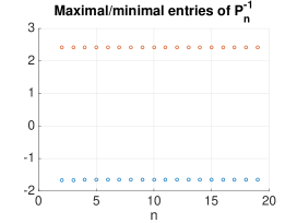
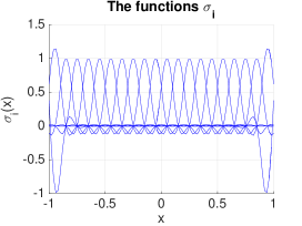
Figure 1: Extremal entries of the inverse collocation matrices $P_{n}^{-1}$ for the quadratic splines from Sect. 4.1.2 depending on $n$ (left) and the associate functions $\sigma_{i}:[-1,1]\to{\mathbb{R}}$, $0\leqslant i\leqslant n+1$, for $n=20$ (right)

Cubic splines

In contrast, let us next construct positivity preserving projection methods as follows:

Corollary 4.8 (cubic splines)

The piecewise defined cubic spline

$$(\Pi_{n}u)(x):= \left(1-3(\tfrac{x-x_{i}}{h_{i}})^{2}+2(\tfrac{x-x_{i}}{h_{i}})^{3}\right)u(x_{i})$$ (4.10)

$$+\left(3(\tfrac{x-x_{i}}{h_{i}})^{2}-2(\tfrac{x-x_{i}}{h_{i}})^{3}\right)u(x_{i+1})\quad\text{for all }x\in[x_{i},x_{i+1}],\,0\leqslant i<n$$

yields a $C[a,b]_{+}^{d}$-positive projection $\Pi_{n}:C[a,b]^{d}\to C^{1}[a,b]^{d}$ satisfying the estimate $\left\|\Pi_{n}\right\|_{L(C[a,b]^{d})}\leqslant 2$.

Although (4.10) gives rise to a positivity preserving spline, its derivative vanishes in all the collocation points $x_{j}$ and thus $\Pi_{n}u$ has rather unpleasant approximation properties. This is also exemplified by a low convergence rate in numerical simulations (see Ex. 5.2) based on (4.10). [Proof.] (I) Given nonnegative real numbers $s_{0},\ldots,s_{n}$, the cubic $C^{1}$-spline $s:[0,1]\to{\mathbb{R}}$, piecewise defined as

$$s(x)=s_{i}+(x-x_{i})m_{i} +(\tfrac{x-x_{i}}{h_{i}})^{2}\left(3(s_{i+1}-s_{i})-h_{i}(2m_{i}+m_{i+1})\right)$$

$$+(\tfrac{x-x_{i}}{h_{i}})^{3}\left(h_{i}(m_{i}+m_{i+1})-2(s_{i+1}-s_{i})\right)$$

for $x\in[x_{i},x_{i+1}]$, $0\leqslant i<n$ is investigated in [21]. It satisfies the interpolation conditions $s(x_{i})=s_{i}$, as well as $s^{\prime}(x_{i})=m_{i}$ for $0\leqslant i\leqslant n$, where $m_{i}\in{\mathbb{R}}$ are free parameters. According to [21, Thm. 4], the spline $s$ is nonnegative on the interval $[0,1]$ if and only if $(m_{i},m_{i+1})\in W_{i}(u)$ holds for all $0\leqslant i<n$, where

$$W_{i}:= \left\{(x,y)\in{\mathbb{R}}^{2}:\,-3s_{i}\leqslant h_{i+1}x,\,h_{i+1}y\leqslant 3s_{i+1}\right\}$$

$$\cup\{(x,y)\in{\mathbb{R}}^{2}:\,0\leqslant 36s_{i}s_{i+1}(x^{2}+xy+y^{2}-3\tau_{i+1}(x+y)+3\tau_{i+1}^{2})$$

$$+3(s_{i+1}x-s_{i}y)(2h_{i+1}xy-3s_{i+1}x+3s_{i}y)$$

$$+4h_{i+1}(s_{i+1}x^{3}-s_{i}y^{3})-h_{i+1}^{2}x^{2}y^{2}\}$$

with $\tau_{i+1}:=\tfrac{s_{i+1}-s_{i}}{h_{i}}$. In particular, choosing $m_{i}:=0$ for all $0\leqslant i\leqslant n$ yields the inclusion $(0,0)\in W_{i}$ and a nonnegative spline

$$s(x)=(1-3\theta^{2}+2\theta^{3})s_{i}+(3\theta^{2}-2\theta^{3})s_{i+1}\quad\text{for all }x\in[x_{j},x_{j+1}],$$

where $\theta:=\tfrac{x-x_{i}}{h_{i}}\in[0,1]$.
(II) Let $u\in C(\Omega)^{d}_{+}$, which by Lemma 2.3(a) means that $0\leqslant\left\langle u(x),y^{\prime}\right\rangle$ for all $x\in[a,b]$, $y^{\prime}\in Y_{+}^{\prime}$. Then the nonnegativity of the spline from step (I) yields

$$\left\langle(\Pi_{n}u)(x),y^{\prime}\right\rangle\stackrel{{\scriptstyle\eqref{corspline1}}}{{=}}(1-3\theta^{2}+2\theta^{3})\left\langle u(x_{i}),y^{\prime}\right\rangle+(3\theta^{2}-2\theta^{3})\left\langle u(x_{i+1}),y^{\prime}\right\rangle\geq 0$$

for all $x\in[x_{i},x_{i+1}]$, $0\leqslant i<n$. Lemma 2.3(a) guarantees $\Pi_{n}u\in C(\Omega)^{d}_{+}$, that is the positivity claim for $\Pi_{n}$. Finally, the estimate

$$(\pi_{n}u)(x)=(\underbrace{1-3\theta^{2}+2\theta^{3}}_{\in[0,1]})u(x_{i})+(\underbrace{3\theta^{2}-2\theta^{3}}_{\in[0,1]})u(x_{i+1})\quad\text{for all }x\in[x_{i},x_{i+1}]$$

implies $\left|(\pi_{n}u)(x)\right|\leqslant 2\left\|u\right\|_{\infty}$ for all $x\in[a,b]$ and $u\in C[a,b]$. Keeping an eye on (4.4) this leads to the claimed norm estimate for the projections $\Pi_{n}$. ∎

Remark 4.9 (positivity preserving splines)

The above Cor. 4.8 is based on the idea to apply positivity preserving interpolation methods. Besides the cubic $C^{1}$-splines from [21], this can alternatively be done using the rational splines of order $\geq 3$ constructed in [20, 23], where the latter reference provides even error estimates. Via bivariate splines this approach also extends to higher-dimensional domains $\Omega$.

4.1.3 sinc-Collocation

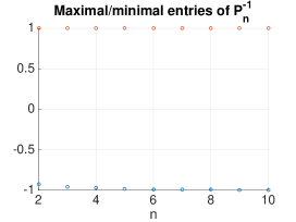
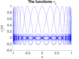
Figure 2: Extremal entries of the inverse collocation matrices $P_{n}^{-1}$ for the $\operatorname{sinc}$-basis from Sect. 4.1.3 depending on $n$ (left) and the associate functions $\sigma_{i}:[-1,1]\to{\mathbb{R}}$, $-n\leqslant i\leqslant n$, for $n=10$ and $\tfrac{\delta}{\alpha}=1$ (right)

Collocation methods based on the cardinal sine function

$$\operatorname{sinc}:{\mathbb{R}} \to{\mathbb{R}}, \operatorname{sinc}x :=\begin{cases}\tfrac{\sin(\pi x)}{\pi x},&x\neq 0,\\ 1,&x=0\end{cases}$$

are discussed in [22]. They require the $\tanh$-transformation $\phi:{\mathbb{R}}\to(a,b)$

$$\phi(x) :=\tfrac{a+b}{2}+\tfrac{b-a}{2}\tanh\left(\tfrac{x}{2}\right), \phi^{-1}(x) :=\ln\tfrac{x-a}{b-x}$$

(with inverse). In order to approximate functions $u:[a,b]\to{\mathbb{R}}$ choose some $\delta\in(0,\pi)$ so that $(a,b)\subseteq D:=\bigl{\{}z\in{\mathbb{C}}:\,\bigl{|}\arg\tfrac{z-a}{b-z}\bigr{|}<\delta\bigr{\}}$ holds and assume $u$ is the restriction of a homomorphic function $u:D\to{\mathbb{C}}$ satisfying the growth condition $\left|u(z)\right|\leqslant C\left|(z-a)(z-b)\right|^{\alpha}$ for all $z\in D$ with reals $C,\alpha>0$. Given $n\in{\mathbb{N}}$, $h:=\sqrt{\tfrac{\pi\delta}{\alpha n}}$ and $S(j,h)(x):=\operatorname{sinc}\tfrac{x-jh}{h}$, we introduce the $d_{n}:=2n+3$ basis functions

$$\phi_{-(n+1)}(x) :=\tfrac{b-x}{b-a}, \phi_{i}(x) :=S(i,h)(\phi^{-1}(x))\quad\text{for all }\left|i\right|\leqslant n, \phi_{n+1}(x) :=\tfrac{x-a}{b-a}$$

with the $2n+3$ collocation points

$$x_{j}:=\begin{cases}a,&j=-n-1,\\ \phi(jh),&\left|j\right|\leqslant n,\\ b,&j=n+1.\end{cases}$$

This yields the nonnegative collocation matrix $P_{n}:=(\phi_{i}(x_{j}))_{i,j=-n-1}^{n+1}$ given by

$$P_{n} =\begin{pmatrix}1&\tfrac{b-x_{-n}}{b-a}&\ldots&\tfrac{b-x_{n}}{b-a}&0\\ 0&1&\ldots&0&0\\ \vdots&&\ddots&&\vdots\\ 0&0&\ldots&1&0\\ 0&\tfrac{x_{-n}-a}{b-a}&\ldots&\tfrac{x_{n}-a}{b-a}&1\\ \end{pmatrix}\in{\mathbb{R}}^{(2n+3)\times(2n+3)}.$$

Fig. 2 shows the extremal entries of $P_{n}^{-1}$ depending on $n\geq 2$. Having positive and negative entries in $P_{n}^{-1}$, Thm. 4.3 fails to apply for $\operatorname{sinc}$-collocation.

4.2 Bubnov-Galerkin methods

For a second class of projection methods, assume $X(\Omega)=L^{2}(\Omega)$ and that $\left\{\phi_{1},\ldots,\phi_{d_{n}}\right\}$ forms a basis of a subspace $X_{n}\subset L^{2}(\Omega)$. With the inner product

$$(u,v):=\int_{\Omega}u(y)v(y)\,{\mathrm{d}}\mu(y)$$ (4.11)

we require orthogonality $(\pi_{n}u-u,\phi_{i})=0$ for $1\leqslant i\leqslant d_{n}$ leading to functionals $\psi_{i}^{\prime}(u)=(u,\phi_{i})$. This results in the positively definite Gramian matrix

$$P_{n}=((\phi_{j},\phi_{i}))_{i,j=1}^{d_{n}}.$$

Theorem 4.10 (positivity of $\Pi_{n}$ on $L^{2}(\Omega)^{d}$)

Assume that every basis element $\phi_{i}:\Omega\to{\mathbb{R}}$, $1\leqslant i\leqslant d_{n}$, has nonnegative values. If the Gramian matrix $P_{n}$ is monomial, then $\Pi_{n}$ is $L^{2}(\Omega)_{+}^{d}$-positive.

[Proof.] Let $u\in L^{2}(\Omega)^{d}$, $0\prec u$ and $y^{\prime}\in Y_{+}^{\prime}$. Thanks to Lemma 2.9(a) this implies $0\leqslant\langle\!\!\langle u(y),y^{\prime}\rangle\!\!\rangle$ for $\mu$-a.a. $y\in\Omega$. Since the Gramian matrix $P_{n}$ is assumed to be monomial, we obtain from [13, p. 2, Thm. 1.1] that the inverse is nonnegative. Hence, if we write $\phi_{j}^{\prime}(u)=((u_{k},\phi_{j}))_{k=1}^{d}$, then (4.1) implies

$$\langle\!\!\langle(\Pi_{n}u)(x),y^{\prime}\rangle\!\!\rangle =\langle\!\!\langle\sum_{j=1}^{d_{n}}\phi_{j}^{\prime}(u)\phi_{j}(x),y^{\prime}\rangle\!\!\rangle=\sum_{j=1}^{d_{n}}\phi_{j}(x)\langle\!\!\langle\phi_{j}^{\prime}(u),y^{\prime}\rangle\!\!\rangle$$

$$=\sum_{j=1}^{d_{n}}\phi_{j}(x)\langle\!\!\langle\sum_{i=1}^{d_{n}}(P_{n}^{-1})_{ij}\int_{\Omega}u(y)\phi_{i}(y)\,{\mathrm{d}}\mu(y),y^{\prime}\rangle\!\!\rangle$$

$$=\sum_{i=1}^{d_{n}}\int_{\Omega}\phi_{i}(y)\underbrace{\langle\!\!\langle u(y),y^{\prime}\rangle\!\!\rangle}_{\geq 0}\,{\mathrm{d}}\mu(y)\sum_{j=1}^{d_{n}}\phi_{j}(x)(P_{n}^{-1})_{ij}\geq 0$$

for all $x\in\Omega$ by assumption. Therefore, Lemma 2.9(a) yields the claim. ∎

Corollary 4.11

For orthogonal bases $\left\{\phi_{1},\ldots,\phi_{d_{n}}\right\}$ consisting of nonnegative functions the projection $\Pi_{n}$ is $L^{2}(\Omega)_{+}^{d}$-positive.

[Proof.] Because $\left\{\phi_{1},\ldots,\phi_{d_{n}}\right\}$ is orthogonal, the Gramian matrix is diagonal with positive entries along the diagonal, i.e. it is monomial. ∎

Corollary 4.12

Let Hypothesis $(L^{2})$ hold with a monomial Gramian matrix $P_{n}$. If ${\mathscr{K}}$ is $L^{2}(\Omega)_{+}^{d}$-positive, then also the compositions $\Pi_{n}{\mathscr{K}}\in L(L^{2}(\Omega),X_{n})$ and ${\mathscr{K}}\Pi_{n}\in L(L^{2}(\Omega)^{d}$) are $L^{2}(\Omega)_{+}^{d}$-positive.

[Proof.] We refer to Cor. A.2. ∎

In the following subsections we endow $\Omega=[a,b]$ with a grid (4.7).

4.2.1 Piecewise constant functions in ${\mathbb{R}}^{\kappa}$

The grid (4.7) breaks $\Omega=[a,b]$ into the subintervals $[x_{j-1},x_{j}]$ of length $h_{j}$, $1\leqslant j\leqslant n$. For the ansatz space

$$X_{n}:=\{u\in L^{2}[a,b]:\,u\text{ is constant on }[x_{j},x_{j+1}],0\leqslant j<n\}$$

of piecewise constant functions the characteristic functions $\phi_{j}:=\chi_{[x_{j-1},x_{j}]}$, $1\leqslant j\leqslant n$, establish an orthogonal basis yielding the diagonal Gramian matrix $P_{n}:=\operatorname{diag}(h_{0},\ldots,h_{n-1}).$ In particular, Cor. 4.11 applies and yields a positive Bubnov-Galerkin method with orthogonal projections

$$\Pi_{n}u=\sum_{j=1}^{n}\frac{1}{h_{j-1}}\int_{x_{j-1}}^{x_{j}}u(y)\,{\mathrm{d}}y\chi_{[x_{j-1},x_{j}]}.$$ (4.12)

Concerning an extension to rectangles $\Omega:=[a_{1},b_{1}]\times\ldots\times[a_{\kappa},b_{\kappa}]$ we proceed as follows: Subdivide each interval $[a_{j},b_{j}]$ into $n$ subintervals $I_{i}^{j}$. With the corresponding characteristic functions $\phi_{i}^{j}=\chi_{I_{i}^{j}}:[a_{j},b_{j}]\to{\mathbb{R}}_{+}$, $1\leqslant i\leqslant n$, multivariable versions read as

$$\phi_{\iota}(x):=\prod_{j=1}^{\kappa}\phi_{\iota_{j}}^{j}(x_{j})\text{ for }x=(x_{1},\ldots,x_{\kappa})\in\Omega,\,\iota=(\iota_{1},\ldots,\iota_{\kappa})\in\left\{1,\ldots,n\right\}^{\kappa}.$$

Given this, choose $\left\{\phi_{\iota}:\Omega\to{\mathbb{R}}_{+}\mid\iota\in\left\{1,\ldots,n\right\}^{\kappa}\right\}$ as basis of $X_{n}\subset L^{p}(\Omega)$ having the dimension $d_{n}=n^{\kappa}$.

Differing from their convenient role in collocation methods (cf. Ex. 4.6), piecewise linear functions do not preserve positivity.

4.2.2 Piecewise linear functions

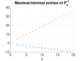
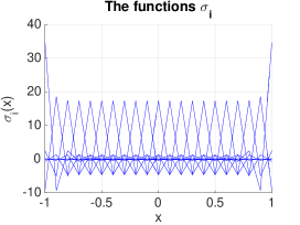
Figure 3: Extremal entries of the inverse Gramian matrices $P_{n}^{-1}$ for piecewise affine basis functions from Sect. 4.2.2 depending on $n$ (left), as well as the associate functions $\sigma_{i}:[-1,1]\to{\mathbb{R}}$, $0\leqslant i\leqslant n$, for $n=20$

With the above notation, consider the ansatz space

$$X_{n}:=\left\{u\in L^{2}[a,b]:\,u\text{ is affine on }[x_{j},x_{j+1}],0\leqslant j<n\right\}$$

of piecewise affine functions. The hat functions $\phi_{j}:[a,b]\to{\mathbb{R}}$ from Ex. 4.6 constitute a basis yielding the tridiagonal $(n+1)\times(n+1)$-Gramian matrix

$$P_{n}=\frac{1}{6}\begin{pmatrix}2h_{0}&h_{0}&&&\\ h_{0}&2(h_{0}+h_{1})&h_{1}&&\\ &\ddots&\ddots&\ddots&\\ &&h_{n-2}&2(h_{n-2}+h_{n-1})&h_{n-1}\\ &&&h_{n-1}&2h_{n-1}\end{pmatrix}$$

(cf. [9, p. 104, Rem. 4.5.26]). Now Cor. 4.11 does not apply, because as illustrated in Fig. 3, the entries of $P_{n}^{-1}$ are positive and negative.

Example 4.13

For simplicity we restrict to $h_{j}=\tfrac{b-a}{n}$ and obtain

$$P_{n}=\frac{b-a}{6n}\begin{pmatrix}2&1&&&&\\ 1&4&1&&&\\ &\ddots&\ddots&\ddots&\\ &&1&4&1\\ &&&1&2\end{pmatrix}.$$

as the Gramian matrix. For $x\in(a,a+h]$ one has

$$(\pi_{n}u)(x)\stackrel{{\scriptstyle\eqref{noproj}}}{{=}} \sum_{j=0}^{n}\phi_{j}^{\prime}(u)\phi_{j}(x)=\phi_{0}^{\prime}(u)\phi_{0}(x)+\phi_{1}^{\prime}(u)\phi_{1}(x)$$

$$\stackrel{{\scriptstyle\eqref{nolgs}}}{{=}} \left((P_{n}^{-1})_{11}(u,\phi_{0})+(P_{n}^{-1})_{12}(u,\phi_{1})\right)\phi_{0}(x)$$

$$+\left((P_{n}^{-1})_{21}(u,\phi_{0})+(P_{n}^{-1})_{22}(u,\phi_{1})\right)\phi_{1}(x)$$

$$= \left((P_{n}^{-1})_{11}\phi_{0}(x)+(P_{n}^{-1})_{21}\phi_{1}(x)\right)(u,\phi_{0})$$

$$+\left((P_{n}^{-1})_{12}\phi_{0}(x)+(P_{n}^{-1})_{22}\phi_{1}(x)\right)(u,\phi_{1})$$

and in particular with the characteristic function $u:=\chi_{[a,a+\theta h]}\in L^{p}[a,b]_{+}$ and $\theta\in(0,1)$ it results from (4.11) that $(u,\phi_{0})=\tfrac{h\theta}{2}(2-\theta)$, $(u,\phi_{1})=\tfrac{h\theta}{2}\theta$. We consequently arrive at

$$(\pi_{n}u)(x)= \tfrac{h\theta}{2}\left[\left((P_{n}^{-1})_{11}\phi_{0}(x)+(P_{n}^{-1})_{21}\phi_{1}(x)\right)(2-\theta)\right.$$

$$+\left.\left((P_{n}^{-1})_{12}\phi_{0}(x)+(P_{n}^{-1})_{22}\phi_{1}(x)\right)\theta\right]$$

and hence, if we choose $\theta>0$ close to $0$ and $x\leqslant a+h$ close to $a+h$ (where $\phi_{0}$ has values near $0$ and $\phi_{1}$ near 1, cf. (4.8)), then the sign of $(\pi_{n}u)(x)$ is determined by the entry $(P_{n}^{-1})_{21}$. Now by Lemma B.1 one has $(P_{n}^{-1})_{21}<0$ and thus there exists an interval $[a+h_{0},a+h]$, $h_{0}\in(0,h)$ on which $(\pi_{n}u)(x)$ is negative, that is $\pi_{n}u\not\in L^{2}[a,b]_{+}$.

5 Applications

5.1 Dispersal kernels

In order to describe the dispersal stage in ecological models [15], various real-valued functions $k_{ij}:\Omega^{2}\to{\mathbb{R}}_{+}$ are used as entries in corresponding matrix-valued kernels $K:\Omega^{2}\to{\mathbb{R}}^{d\times d}$ for Fredholm operators ${\mathscr{K}}$; thus one speaks of dispersal kernels and chooses the Lebesgue measure $\mu=\lambda_{\kappa}$. Often the functions $k=k_{ij}$ are symmetric, i.e. $k(x,y)=k(y,x)$, or of convolution form $k(x,y)=\tilde{k}(x-y)$ for all $x,y\in\Omega$ with an even function $\tilde{k}:{\mathbb{R}}^{\kappa}\to{\mathbb{R}}_{+}$. Given a dispersal rate $\alpha>0$ and the Euclidean norm $\left|\cdot\right|$ on ${\mathbb{R}}^{\kappa}$ typical choices are listed in Tab. 1.

kernel	$\tilde{k}(x)$
Gauß	$\tfrac{1}{\sqrt{2\pi\alpha^{2}}}\exp\left(-\tfrac{1}{2\alpha^{2}}\left|x\right|^{2}\right)$
Cauchy	$\tfrac{\alpha}{\pi(\alpha^{2}+\left|x\right|^{2})}$
Laplace	$\tfrac{1}{2\alpha}\exp\left(-\tfrac{1}{\alpha}\left|x\right|\right)$
exponential square root	$\frac{1}{4\alpha}\exp\left(-\sqrt{\tfrac{1}{\alpha}\left|x\right|}\right)$
top-hat	$\tfrac{1}{2\alpha}\chi_{B_{\alpha}(0)}(\left|x\right|)$
tent	$\tfrac{1}{\alpha}\max\left\{0,1-\tfrac{1}{\alpha}\left|x\right|\right\}$

Table 1: List of dispersal kernels satisfying $\int_{{\mathbb{R}}}\tilde{k}(y)\,{\mathrm{d}}y=1$ for $\kappa=1$

The kernels from Tab. 1 satisfy Hypothesis $(L)$ (whose limit relation moreover holds uniformly in $x_{0}$), as well as Hypothesis $(L^{2})$. Consequently, the resulting Fredholm operator ${\mathscr{K}}u=\int_{\Omega}k(\cdot,y)u(y)\,{\mathrm{d}}y$ acting on $C(\Omega)$ resp. $L^{2}(\Omega)$ is even compact. In case $Y_{+}={\mathbb{R}}_{+}$ these kernels yield positive operators ${\mathscr{K}}$ due to Thm. 2.7 resp. 2.12. On the space $X(\Omega)=C(\Omega)$, besides for the top-hat and the tent kernel, ${\mathscr{K}}$ is even strongly positive. Yet, for sufficiently large dispersal rates $\alpha$ also the top-hat and tent kernel yield a strongly positive ${\mathscr{K}}$, i.e. provided the condition $\Omega\subseteq B_{\alpha}(y)$ for all $y\in\Omega$ holds.

Now we return to matrix-valued kernels in ${\mathscr{K}}$: Here criteria for positivity can be derived from Ex. 2.4 and 2.5. With vectors $e_{i}\in{\mathbb{R}}^{d}$ spanning $Y_{+}\subset{\mathbb{R}}^{d}$ and $e_{j}^{\prime}\in{\mathbb{R}}^{d}$, a kernel $K(x,y)\in{\mathbb{R}}^{d\times d}$ is

• $Y_{+}$-positive $\Leftrightarrow 0\leqslant\langle\!\!\langle K(x,y)e_{i},e_{j}^{\prime}\rangle\!\!\rangle$,

• strictly $Y_{+}$-positive $\Leftrightarrow 0\leqslant\langle\!\!\langle K(x,y)e_{i},e_{j}^{\prime}\rangle\!\!\rangle$ and $K(x,y)$ is $Y_{+}$-injective,

• strongly $Y_{+}$-positive $\Leftrightarrow 0<\langle\!\!\langle K(x,y)e_{i},e_{j}^{\prime}\rangle\!\!\rangle$

holds for all $1\leqslant i,j\leqslant d$, $x\in\Omega$ and $\mu$-a.a. $y\in\Omega$.

If a cone $Y_{+}$ is an orthant as in Ex. 2.5, then $\langle\!\!\langle K(x,y)e_{i},e_{j}^{\prime}\rangle\!\!\rangle=\varsigma_{i}\varsigma_{j}k_{ij}(x,y)$ implies that $K(x,y)$ is

• $Y_{+}$-positive $\Leftrightarrow\varsigma_{i}\varsigma_{j}k_{ij}(x,y)\geq 0$,

• strictly $Y_{+}$-positive $\Leftrightarrow\varsigma_{i}\varsigma_{j}k_{ij}(x,y)\geq 0$ and $K(x,y)$ is $Y_{+}$-injective,

• strongly $Y_{+}$-positive $\Leftrightarrow\operatorname{sgn}k_{ij}(x,y)=\varsigma_{i}\varsigma_{j}$

for all $1\leqslant i,j\leqslant d$, $x\in\Omega$ and $\mu$-a.a. $y\in\Omega$.

5.2 Krein-Rutman eigenfunctions

Let $X(\Omega)$ be a Banach space of real-valued functions over $\Omega$. Given a compact Fredholm operator ${\mathscr{K}}\in L(X(\Omega)^{d})$, the Krein-Rutman Thm. A.3 provides conditions guaranteeing that its spectral radius $r({\mathscr{K}})>0$ is the dominant eigenvalue with an associate nonnegative eigenfunction $u^{\ast}\in X(\Omega)^{d}$. In this section, we investigate in which sense this property is preserved under discretization.

For this purpose, consider an abstract eigenvalue problem

$${\mathscr{K}}u=\lambda u\quad\text{in }X(\Omega)^{d}$$ (5.1)

for a Fredholm operator ${\mathscr{K}}$. Numerical approaches to (5.1) approximate $(\lambda,u)\in{\mathbb{C}}\times X(\Omega)$ by eigenpairs $(\lambda_{n},\hat{v}^{n})\in{\mathbb{C}}\times{\mathbb{R}}^{dN_{n}}$ of related problems

$$K^{n}\hat{v}^{n}=\lambda_{n}\hat{v}^{n},$$ (5.2)

where the matrices $K^{n}\in{\mathbb{R}}^{dN_{n}\times dN_{n}}$ depend on the particular discretization method. Nevertheless, $K^{n}$ consists of block matrices

$$K^{n} :=\begin{pmatrix}K_{11}&\ldots&K_{1d}\\ \vdots&&\vdots\\ K_{d1}&\ldots&K_{dd}\end{pmatrix}, \hat{v}^{n} :=\begin{pmatrix}v_{1}\\ \vdots\\ v_{d}\end{pmatrix},$$

with also $v_{i}\in{\mathbb{R}}^{N_{n}}$ and $K_{ij}\in{\mathbb{R}}^{N_{n}\times N_{n}}$ depending on the method.

Nevertheless, in our numerical computations we rely on the Matlab functions eig to approximate the dominant eigenvalue of $K^{n}$ and eigs when also the corresponding eigenvectors are of interest.

5.2.1 Nyström methods

Let $X(\Omega)=C(\Omega)$ and ($Q_{n}$) be a quadrature rule. Replacing ${\mathscr{K}}$ in (5.1) by the discrete Fredholm operator (3.2) yields

$$\sum_{j_{2}=0}^{q_{n}}w_{j_{2}}K(x,\eta_{j_{2}})u(\eta_{j_{2}})=\lambda u(x)\quad\text{for all }x\in\Omega.$$

If we now set $x=\eta_{j_{1}}$ for $0\leqslant j_{1}\leqslant q_{n}$, then one obtains a matrix $K^{n}$ as in relation (5.2) with $N_{n}:=q_{n}+1$ and the blocks

$$K_{i_{1}i_{2}}=(w_{j_{2}}k_{i_{1}i_{2}}(\eta_{j_{1}},\eta_{j_{2}}))_{j_{1},j_{2}=0}^{q_{n}}\quad\text{for all }1\leqslant i_{1},i_{2}\leqslant d.$$

For simplicity we retreat to real-valued continuous kernels $K:\Omega\times\Omega\to(0,\infty)$ and the solid cone $Y_{+}:={\mathbb{R}}_{+}$. Then ${\mathscr{K}}$ is strongly positive by Thm. 2.7(b) and the Krein-Rutman Thm. A.3(b) yields that the spectral radius $r({\mathscr{K}})>0$ is the dominant eigenvalue with eigenfunction $u^{\ast}\in C(\Omega)_{+}^{\circ}$. If all the quadrature weights are positive, then a discrete Fredholm operator ${\mathscr{K}}^{n}$ from (3.2) is

• strongly positive on $C(\Omega_{n})$ (cf. Rem. 3.3) and thus Thm. A.3(b) applies,

• positive on $C(\Omega)$ (due to Thm. 3.4), where Thm. A.3(a) applies.

In any case, one obtains the dominant eigenpair $(r({\mathscr{K}}^{n}),\hat{v}^{n})$ from the equation (5.2) and as dominant eigenfunction $u_{n}^{\ast}\in C(\Omega)$ we use the Nyström interpolate

$$u_{n}^{\ast}(x):=\frac{1}{r({\mathscr{K}}^{n})}\sum_{j=0}^{q_{n}}w_{j}K(x,\eta_{j})\hat{v}_{j}^{n}\quad\text{for all }x\in\Omega.$$

The positivity of the numerically obtained eigenfunction $u_{n}^{\ast}$ is confirmed by

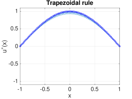
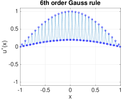
Figure 4: Nyström discretization to approximate the dominant positive eigenfunction of the Gauß kernel with $\alpha=0.01$ based on quadrature rules with $90$ nodes. The dots represent the values $u_{n}^{\ast}(\eta)$, $\eta\in\Omega_{n}$

Example 5.1 (Gauß kernel)

We apply different Nyström methods to the Fredholm operator

$$({\mathscr{K}}u)(x)=\frac{1}{\sqrt{2\pi\alpha^{2}}}\int_{-1}^{1}e^{-\tfrac{(x-y)^{2}}{2\alpha^{2}}}u(y)\,{\mathrm{d}}y$$

with the dispersal rate $\alpha=0.01$ over $\Omega=[-1,1]$. The corresponding dominant eigenfunctions (as Nyström interpolates) for the Trapezoidal rule (C.2) and $6$th order Gauß rule (C.4) are illustrated in Fig. 4 (each with $90$ notes). Both cases yield strongly positive eigenfunctions (although hardly visible in Fig. 4, one has $u^{\ast}(x)>0$ for $x\in\left\{-1,1\right\}$), but the Gauß discretizations exhibit a strongly oscillatory behavior. This is due to the fact that the used number of nodes $(q_{n}=89)$ is small in comparison to the dispersal rate $(\alpha=0.01)$. Oscillations become weaker when increasing $q_{n}$.
For the Milne rule (C.3) this situation changes, since it involves negative weights. Indeed, the resulting discrete Fredholm operator ${\mathscr{K}}^{n}$ is not positive and the Krein-Rutman Thm. A.3 does not apply. As illustrated in Fig. 5 the eigenfunction corresponding to the eigenvalue with maximal real part can have varying signs. Numerical experiments exhibit that this sign changing property persists until the number of nodes is larger than $146$.

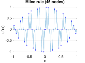
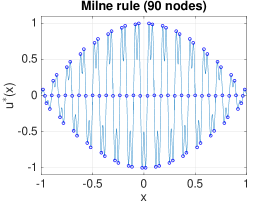
Figure 5: Nyström discretization to approximate the dominant positive eigenfunction of the Gauß kernel with $\alpha=0.01$ based on Milne’s rule (C.3) with with $45$ nodes (left) and $90$ nodes (right).

5.2.2 Projection methods

Based on the ansatz space $X_{n}=\operatorname{span}\left\{\phi_{1},\ldots,\phi_{d_{n}}\right\}$ we aim to approximate solutions to eigenvalue problems (5.1) numerically. Thereto, replace $u$ in (5.1) by $u^{n}=\Pi_{n}u$ given as in (4.3). This leads to a discretized version

$${\mathscr{K}}^{n}u^{n}=\lambda_{n}u^{n}\quad\text{in }X_{n}^{d}$$ (5.3)

with ${\mathscr{K}}^{n}={\mathscr{K}}\Pi_{n}$ in order to obtain approximations $(\lambda_{n},u^{n})$, $u^{n}\in X_{n}^{d}$, to an eigenpair $(\lambda,u)$, $u\in X(\Omega)^{d}$, of (5.1). Note that for a solution $u^{n}\in X_{n}^{d}$ of the discretized problem (5.3) one has ${\mathscr{K}}^{n}u^{n}\in X_{n}^{d}$.

Similarly, one proceeds for spatial discretization of Fredholm equations of the first and second kind (cf. [3, 9]).

For a matrix-valued kernel $K(x,y)$ define the Fredholm operators

$${\mathscr{K}}_{i_{1},i_{2}} \in L(X(\Omega)), {\mathscr{K}}_{i_{1}i_{2}}u :=\int_{\Omega}k_{i_{1}i_{2}}(\cdot,y)u(y)\,{\mathrm{d}}y\quad\text{for all }1\leqslant i_{1},i_{2}\leqslant d.$$

In this notation, the eigenvalue problem (5.1) is equivalent to the relation $\sum_{i_{2}=1}^{d}{\mathscr{K}}_{i_{1}i_{2}}u_{i_{2}}=\lambda u_{i_{1}}$ for $1\leqslant i_{1}\leqslant d$ and in order to arrive at the spatially discretized problem (5.3), we insert $u_{i_{2}}=\sum_{j_{1}=1}^{d_{n}}v_{i_{2}}^{j_{1}}\phi_{j_{1}}$ with $v_{i_{2}}^{j_{1}}\in{\mathbb{R}}$. Applying the functional $\phi_{j_{2}}^{\prime}$ yields

$$\sum_{i_{2}=1}^{d}\sum_{j_{1}=1}^{d_{n}}\phi_{j_{2}}^{\prime}({\mathscr{K}}_{i_{1}i_{2}}\phi_{j_{1}})v_{i_{2}}^{j_{1}}=\lambda_{n}v_{i_{1}}^{j_{2}}\quad\text{for all }1\leqslant i_{1}\leqslant d,\,1\leqslant j_{2}\leqslant d_{n}.$$

This is equivalent to an eigenproblem (5.2) with $N_{n}=d_{n}$ and the blocks

$$K_{i_{1}i_{2}} :=\begin{pmatrix}\phi_{1}^{\prime}({\mathscr{K}}_{i_{1}i_{2}}\phi_{1})&\ldots&\phi_{1}^{\prime}({\mathscr{K}}_{i_{1}i_{2}}\phi_{d_{n}})\\ \vdots&&\vdots\\ \phi_{d_{n}}^{\prime}({\mathscr{K}}_{i_{1}i_{2}}\phi_{1})&\ldots&\phi_{d_{n}}^{\prime}({\mathscr{K}}_{i_{1}i_{2}}\phi_{d_{n}})\end{pmatrix}, v_{i_{1}} :=\begin{pmatrix}v_{i_{1}}^{1}\\ \vdots\\ v_{i_{1}}^{d_{n}}\end{pmatrix}$$

for all $1\leqslant i_{1},i_{2}\leqslant d$. On this basis, the eigenfunctions of (5.3) become

$$u^{n}=\sum_{j=1}^{d_{n}}\phi_{j}\begin{pmatrix}v_{1}^{j}\\ \vdots\\ v_{d}^{j}\end{pmatrix}.$$

In order to be more specific, let us emphasize the subsequent projection methods with an interval $\Omega=[a,b]$ on a grid (4.7).

Collocation with Lagrange bases: Lagrange bases $\left\{\phi_{1},\ldots,\phi_{d_{n}}\right\}$ lead to blocks

$$K_{i_{1}i_{2}}=\int_{\Omega}\begin{pmatrix}k_{i_{1}i_{2}}(x_{1},y)\phi_{1}(y)&\ldots&k_{i_{1}i_{2}}(x_{1},y)\phi_{d_{n}}(y)\\ \vdots&&\vdots\\ k_{i_{1}i_{2}}(x_{d_{n}},y)\phi_{1}(y)&\ldots&k_{i_{1}i_{2}}(x_{d_{n}},y)\phi_{d_{n}}(y)\\ \end{pmatrix}\,{\mathrm{d}}y.$$

In particular, the bases from Ex. 4.6 (hat functions) and Ex. 4.7 (Lagrange functions) are of the form $\left\{\phi_{0},\ldots,\phi_{n}\right\}$ and thus $d_{n}=n+1$ in (5.2).

Collocation with cubic splines: Use the order-preserving $C^{1}$-spline

$$(\Pi_{n}u)(x):=\kappa_{j}(x)u(x_{j})+\bar{\kappa}_{j}(x)u(x_{j+1})\quad\text{for all }x\in[x_{j},x_{j+1}],\,0\leqslant j<n$$

from Cor. 4.8 with the real coefficients

$$\kappa_{j}(x) :=1-3(\tfrac{x-x_{j}}{h_{j}})^{2}+2(\tfrac{x-x_{j}}{h_{j}})^{3}, \bar{\kappa}_{j}(x) :=3(\tfrac{x-x_{j}}{h_{j}})^{2}-2(\tfrac{x-x_{j}}{h_{j}})^{3},$$

which results in

$$({\mathscr{K}}\Pi_{n}u)(x) =\sum_{j=0}^{n-1}\int_{x_{j}}^{x_{j+1}}K(x,y)\kappa_{j}(y)\,{\mathrm{d}}yu(x_{j})+\sum_{j=0}^{n-1}\int_{x_{j}}^{x_{j+1}}K(x,y)\bar{\kappa}_{j}(y)\,{\mathrm{d}}yu(x_{j+1})$$

for all $x\in[a,b]$. Setting $x=x_{i}$ for $0\leqslant i\leqslant n$ in the ansatz (5.3) combined with the abbreviations $u_{i}:=u(x_{i})$ yields the $n+1$ identities

$$\sum_{j=0}^{n-1}\int_{x_{j}}^{x_{j+1}}K(x_{i},y)\kappa_{j}(y)\,{\mathrm{d}}yu_{j}+\sum_{j=0}^{n-1}\int_{x_{j}}^{x_{j+1}}K(x_{i},y)\bar{\kappa}_{j}(y)\,{\mathrm{d}}yu_{j+1} =\lambda u_{i}$$

for all $0\leqslant i\leqslant n$, which are equivalent to the eigenvalue problem

$$\Bigl{(}\begin{pmatrix}\int_{x_{0}}^{x_{1}}K(x_{0},y)\kappa_{0}(y)\,{\mathrm{d}}y&\ldots&\int_{x_{n-1}}^{x_{n}}K(x_{0},y)\kappa_{n-1}(y)\,{\mathrm{d}}y&0\\ \vdots&&\vdots&\vdots\\ \int_{x_{0}}^{x_{1}}K(x_{n-1},y)\kappa_{0}(y)\,{\mathrm{d}}y&\ldots&\int_{x_{n-1}}^{x_{n}}K(x_{n-1},y)\kappa_{n-1}(y)\,{\mathrm{d}}y&0\\ 0&\ldots&0&0\end{pmatrix}$$

$$+\begin{pmatrix}0&0&\cdots&0\\ 0&\int_{x_{0}}^{x_{1}}K(x_{0},y)\bar{\kappa}_{0}(y)\,{\mathrm{d}}y&\ldots&\int_{x_{n-1}}^{x_{n}}K(x_{0},y)\bar{\kappa}_{n-1}(y)\,{\mathrm{d}}y\\ \vdots&\vdots&&\vdots\\ 0&\int_{x_{0}}^{x_{1}}K(x_{n-1},y)\bar{\kappa}_{0}(y)\,{\mathrm{d}}y&\ldots&\int_{x_{n-1}}^{x_{n}}K(x_{n-1},y)\bar{\kappa}_{n-1}(y)\,{\mathrm{d}}y\\ \end{pmatrix}\Bigr{)}\begin{pmatrix}u_{0}\\ \vdots\\ u_{n-1}\\ u_{n}\end{pmatrix}=\lambda\begin{pmatrix}u_{0}\\ \vdots\\ u_{n-1}\\ u_{n}\end{pmatrix}$$

in ${\mathbb{R}}^{(n+1)d}$. Referring to the formulation (5.2) this gives rise to the blocks

$$K_{i_{1}i_{2}}= \begin{pmatrix}\int_{x_{0}}^{x_{1}}k_{i_{1}i_{2}}(x_{0},y)\kappa_{0}(y)\,{\mathrm{d}}y&\ldots&\int_{x_{n-1}}^{x_{n}}k_{i_{1}i_{2}}(x_{0},y)\kappa_{n-1}(y)\,{\mathrm{d}}y&0\\ \vdots&&\vdots&\vdots\\ \int_{x_{0}}^{x_{1}}k_{i_{1}i_{2}}(x_{n-1},y)\kappa_{0}(y)\,{\mathrm{d}}y&\ldots&\int_{x_{n-1}}^{x_{n}}k_{i_{1}i_{2}}(x_{n-1},y)\kappa_{n-1}(y)\,{\mathrm{d}}y&0\\ 0&\ldots&0&0\end{pmatrix}$$

$$+\begin{pmatrix}0&0&\cdots&0\\ 0&\int_{x_{0}}^{x_{1}}k_{i_{1}i_{2}}(x_{0},y)\bar{\kappa}_{0}(y)\,{\mathrm{d}}y&\ldots&\int_{x_{n-1}}^{x_{n}}k_{i_{1}i_{2}}(x_{0},y)\bar{\kappa}_{n-1}(y)\,{\mathrm{d}}y\\ \vdots&\vdots&&\vdots\\ 0&\int_{x_{0}}^{x_{1}}k_{i_{1}i_{2}}(x_{n-1},y)\bar{\kappa}_{0}(y)\,{\mathrm{d}}y&\ldots&\int_{x_{n-1}}^{x_{n}}k_{i_{1}i_{2}}(x_{n-1},y)\bar{\kappa}_{n-1}(y)\,{\mathrm{d}}y\\ \end{pmatrix}.$$

Bubnov-Galerkin method with piecewise constant basis: One obtains the blocks

$$K_{i_{1}i_{2}}=\int_{\Omega}\int_{\Omega}\begin{pmatrix}k_{i_{1}i_{2}}(x,y)\phi_{1}(y)\phi_{1}(x)&\ldots&k_{i_{1}i_{2}}(x,y)\phi_{d_{n}}(y)\phi_{1}(x)\\ \vdots&&\vdots\\ k_{i_{1}i_{2}}(x,y)\phi_{1}(y)\phi_{d_{n}}(x)&\ldots&k_{i_{1}i_{2}}(x,y)\phi_{d_{n}}(y)\phi_{d_{n}}(x)\end{pmatrix}\,{\mathrm{d}}y\,{\mathrm{d}}x.$$

Because the piecewise constant basis functions $\left\{\phi_{1},\ldots,\phi_{n}\right\}$ from Sect. 4.2.1 have the support $[x_{j},x_{j+1}]$, $0\leqslant j<n$, the integrals simplify to

$$K_{i_{1}i_{2}}=\begin{pmatrix}\int_{x_{0}}^{x_{1}}\int_{x_{0}}^{x_{1}}k_{i_{1}i_{2}}(x,y)\,{\mathrm{d}}y\,{\mathrm{d}}x&\ldots&\int_{x_{0}}^{x_{1}}\int_{x_{n-1}}^{x_{n}}k_{i_{1}i_{2}}(x,y)\,{\mathrm{d}}y\,{\mathrm{d}}x\\ \vdots&&\vdots\\ \int_{x_{n-1}}^{x_{n}}\int_{x_{0}}^{x_{1}}k_{i_{1}i_{2}}(x,y)\,{\mathrm{d}}y\,{\mathrm{d}}x&\ldots&\int_{x_{n-1}}^{x_{n}}\int_{x_{n-1}}^{x_{n}}k_{i_{1}i_{2}}(x,y)\,{\mathrm{d}}y\,{\mathrm{d}}x\end{pmatrix}.$$

$i$	$\alpha_{i}$	$\nu_{i}$	$\lambda^{i}$
$1$	1.0	0.86033358901938	0.5746552163364324
$2$	2.0	1.30654237418881	0.3694054047082261

Table 2: Dominant eigenvalues $\lambda^{i}$ of ${\mathscr{K}}_{i}$ for $L=2$

Finally let us test the above methods by means of

Example 5.2 (Laplace kernel)

Let $\alpha_{1},\alpha_{2}>0$ denote dispersal rates and a mapping $k:\Omega\times\Omega\to(0,\infty)$ be continuous. The Fredholm operator

$${\mathscr{K}}u :=\int_{\Omega}K(\cdot,y)u(y)\,{\mathrm{d}}y, K(x,y) :=\begin{pmatrix}\tfrac{1}{2\alpha_{1}}e^{-\tfrac{|x-y|}{\alpha_{1}}}&-k(x,y)\\ 0&\tfrac{1}{2\alpha_{2}}e^{-\tfrac{|x-y|}{\alpha_{2}}}\end{pmatrix}$$

satisfies Hypothesis $(NL)$ and is compact on $C(\Omega)^{2}$, as well as on $L^{2}(\Omega)^{2}$. The south-east cone $Y_{+}:={\mathbb{R}}_{+}\times(-{\mathbb{R}}_{+})$ is spanned by the vectors $e_{1}:=\binom{1}{0}$, $e_{2}:=-\binom{0}{1}$ and with $e_{i}^{\prime}:=e_{i}$ for $i=1,2$ we consequently obtain

$$\left\langle K(x,y)e_{1},e_{1}^{\prime}\right\rangle =\tfrac{1}{2\alpha_{1}}e^{-\tfrac{|x-y|}{\alpha_{1}}}>0, \left\langle K(x,y)e_{2},e_{1}^{\prime}\right\rangle =k(x,y)>0,$$

$$\left\langle K(x,y)e_{1},e_{2}^{\prime}\right\rangle =0, \left\langle K(x,y)e_{2},e_{2}^{\prime}\right\rangle =\tfrac{1}{2\alpha_{2}}e^{-\tfrac{|x-y|}{\alpha_{2}}}>0.$$

Therefore, the kernel $K(x,y)$ is $Y_{+}$-positive for all $x,y\in\Omega$. Thus, Thm. 2.7 implies that ${\mathscr{K}}$ is $C(\Omega)_{+}^{2}$-positive, while Thm. 2.12 ensures $L^{2}(\Omega)_{+}^{2}$-positivity. With the aid of

$${\mathscr{K}}_{i}u(x):=\frac{1}{2\alpha_{i}}\int_{\Omega}e^{-\tfrac{|x-y|}{\alpha_{i}}}u(y)\,{\mathrm{d}}y\quad\text{for all }x\in\Omega,\,i=1,2$$

we obtain the spectrum $\sigma({\mathscr{K}})=\sigma({\mathscr{K}}_{1})\cup\sigma({\mathscr{K}}_{2})$.
In order to compute the dominant eigenvalue of ${\mathscr{K}}$ numerically, we retreat to intervals $\Omega=[-\tfrac{L}{2},\tfrac{L}{2}]$ for some $L>0$. It is shown in [15, pp. 24–27, Sect. 3.2] that the dominant eigenvalue $\lambda^{i}>0$ of ${\mathscr{K}}_{i}$ and the smallest positive solution $\nu_{i}$ of the transcendental equation $\tan(\tfrac{L}{2\alpha_{i}}\nu)=\tfrac{1}{\nu}$ are related via $\lambda^{i}=\tfrac{1}{1+\nu_{i}^{2}}$. We refer to Tab. 2 for exact values and approximate the dominant eigenvalue with positive collocation methods (piecewise linear, polynomial and spline) and positive Bubnov-Galerkin methods (piecewise constant). This is based on a grid (4.7) with $a=-\tfrac{L}{2}$, $b=\tfrac{L}{2}$ and $x_{j}:=-\tfrac{L}{2}+j\tfrac{L}{n}$, $0\leqslant j\leqslant n$. For the sake of discrete projection methods, the remaining integrals are approximated by the summed midpoint rule (C.1) with the centered nodes $\eta_{i}:=x_{i}-\tfrac{L}{2n}$, $1\leqslant i\leqslant n$.
For $L=2$ and $\alpha_{i}$ as in Tab. 2 we moreover compute the dominant eigenvalue of $K^{n}$ and relate it to the exact eigenvalue $\lambda^{1}\approx 0.5746552163364324$ of ${\mathscr{K}}$. The results of our numerical simulations are illustrated in Fig. 6. Piecewise linear collocation and the Bubnov-Galerkin method with piecewise constant basis functions illustrate quadratic convergence. This is also true for collocation with polynomial basis functions until beginning with $n\approx 25$ computational instabilities become apparent. The positivity preserving collocation based on cubic splines from Cor. 4.8 shows only linear convergence.

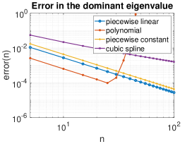
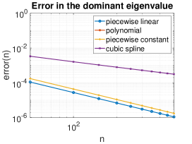
Figure 6: Error in the dominant eigenvalue for piecewise linear collocation $(\circ)$, polynomial collocation ($\bullet$), Bubnov-Galerkin with piecewise constant functions $(+)$ and cubic splines $(\times)$ up to $n=100$ nodes (left) and up to $n=500$ nodes (right)

6 Conclusion

We provided sufficient conditions that positivity properties in a general class of matrix-valued kernels $K$ transfer to Fredholm operators ($F$) over compact domains $\Omega$. In addition, the persistence of this property under Nyström and projection methods is studied. As a result, when solving numerical problems involving such operators, we recommend to restrict to Nyström methods with positive weights. Among the projection methods, collocation with piecewise linear basis functions yields positivity-preserving semi-discretizations and a combination with the Midpoint Rule (C.1) or the Trapezoidal Rule (C.2) leads to a corresponding scheme. Although there are further positivity preserving collocation methods, they have less favorable properties. For Bubnov-Galerkin methods, piecewise constant approximation is suitable and can be combined with e.g. the Midpoint Rule (C.1) in order to arrive at feasible schemes preserving positivity.

Appendix A Cones and positive operators

Let $(X,\left\|\cdot\right\|)$ denote a real Banach space with dual space $X^{\prime}$ and the duality pairing $\left\langle x,x^{\prime}\right\rangle:=x^{\prime}(x)$. A nonempty closed and convex subset $X_{+}\subseteq X$ is called (order) cone, if ${\mathbb{R}}_{+}X_{+}\subseteq X_{+}$ and $X_{+}\cap(-X_{+})=\left\{0\right\}$ hold. Equipped with such a cone one arrives at an ordered Banach space $X$. Let us assume $X_{+}\neq\left\{0\right\}$ throughout and for elements $x,\bar{x}\in X$ we write

$$x\leqslant\bar{x}\quad :\Leftrightarrow\quad\bar{x}-x\in X_{+},$$

$$x<\bar{x}\quad :\Leftrightarrow\quad\bar{x}-x\in X_{+}\setminus\left\{0\right\},$$ (A.1)

$$x\ll\bar{x}\quad :\Leftrightarrow\quad\bar{x}-x\in X_{+}^{\circ};$$

the latter relation requires $X_{+}^{\circ}\neq\emptyset$ and one speaks of a solid cone $X_{+}$. A cone is total, if $X=\overline{X_{+}-X_{+}}$. Solid cones satisfy $X=X_{+}-X_{+}$ and are total.

By means of the dual cone $X_{+}^{\prime}:=\left\{x^{\prime}\in X^{\prime}:\,0\leqslant\left\langle x,x^{\prime}\right\rangle\text{ for all }x\in X_{+}\right\}$ we can characterize the elements of $X_{+}$ and $X_{+}^{\circ}$ as follows:

Lemma A.1

1. $X_{+}^{\prime}\neq\{0\}$ and for every $x\in X$ the following holds:

   $$x\in X_{+} \Leftrightarrow 0\leqslant\left\langle x,x^{\prime}\right\rangle\quad\text{for all }x^{\prime}\in X_{+}^{\prime},$$

   $$x\in X_{+}\setminus\left\{0\right\} \Rightarrow 0<\left\langle x,x_{0}^{\prime}\right\rangle\quad\text{for some }x_{0}^{\prime}\in X_{+}^{\prime}\setminus\left\{0\right\}.$$

2. If $X_{+}$ is solid, then for every $x\in X$ the following holds:

   $$x\in X_{+}^{\circ} \Leftrightarrow 0<\left\langle x,x^{\prime}\right\rangle\quad\text{for all }x^{\prime}\in X_{+}^{\prime}\setminus\left\{0\right\},$$

   $$x\in\partial X_{+} \Rightarrow 0=\left\langle x,x_{0}^{\prime}\right\rangle\quad\text{for some }x_{0}^{\prime}\in X_{+}^{\prime}\setminus\left\{0\right\}.$$ (A.2)

[Proof.] Due to [5, p. 222, Prop. 19.3(a–b)] it remains to verify the direction “$\Leftarrow$” in the first equivalence of (b). Let $0<\left\langle x,x^{\prime}\right\rangle$ for all $x^{\prime}\in X_{+}^{\prime}\setminus\left\{0\right\}$ and we deduce $x\in X_{+}$ from (a). Using the contraposition of (A.2) we derive $x\notin\partial X_{+}$ which implies that $x\in X_{+}^{\circ}$. ∎

A bounded linear mapping $T\in L(X)$ is called

• positive, if $T(X_{+}\setminus\left\{0\right\})\subseteq X_{+}$,

• strictly positive, if $T(X_{+}\setminus\left\{0\right\})\subseteq X_{+}\setminus\left\{0\right\}$,

• strongly positive, if $T(X_{+}\setminus\left\{0\right\})\subseteq X_{+}^{\circ}$.

When working with several cones, we write $X_{+}$-positive etc., in order to indicate a particular cone. We denote $T\in L(X)$ as $X_{+}$-injective, provided

$$N(T)\cap X_{+}=\left\{0\right\}$$

holds. Then $T$ is strictly positive, if and only if it is positive and $X_{+}$-injective. A strongly positive $T$ yields the inclusion $TX_{+}^{\circ}\subseteq X_{+}^{\circ}$.

The positivity properties are preserved under compositions and it holds:

Corollary A.2

Let $X_{+}$ be solid and $T,S\in L(X)$. If $S$ is strictly positive and $T$ is strongly positive, or if $S$ strongly positive and $T$ satisfies $TX_{+}^{\circ}\subseteq X_{+}^{\circ}$, then $TS$ is strongly positive.

[Proof.] This is immediate by definition. ∎

We conclude with a Krein-Rutman theorem suiting our aims (see also [14]):

Theorem A.3 (Krein-Rutman)

Let $T\in L(X)$ be compact.

1. If $X_{+}$ is total and $T$ is positive with $r(T)>0$, then the spectral radius $r(T)$ is an eigenvalue of $T$ with positive eigenvector $x^{\ast}$ (cf. [5, p. 226, Thm. 19.2] or [24, p. 290, Prop. 7.26]).

2. If $X_{+}$ is solid and $T$ is strongly positive, then $T$ has exactly one eigenvector with $0<x^{\ast}$ and $\left\|x^{\ast}\right\|=1$; the corresponding eigenvalue is $r(T)$ and $0\ll x^{\ast}$ (cf. [24, p. 290, Thm. 7.C]).

One calls $x^{\ast}$ a dominant eigenvector (eigenfunction on function spaces $X$).

Appendix B Tridiagonal matrices

Let $n\in{\mathbb{N}}\setminus\left\{1\right\}$ and $a_{1},\ldots,a_{n}$, $b_{1},\ldots,b_{n-1}$, $c_{1},\ldots,c_{n-1}$ be reals with $b_{j}\neq 0$, $1\leqslant j<n$, such that the tridiagonal matrix

$$T:=\begin{pmatrix}a_{1}&b_{1}&&&\\ c_{1}&a_{2}&b_{2}&&\\ &\ddots&\ddots&\ddots&\\ &&c_{n-2}&a_{n-1}&b_{n-1}\\ &&&c_{n-1}&a_{n}\end{pmatrix}$$

is nonsingular. If we recursively introduce the finite sequences

$$d_{n} :=a_{n}, d_{t-1} :=a_{t-1}-\tfrac{b_{t-1}c_{t-1}}{d_{t}}\quad\text{for all }t=n,\ldots,2,$$

$$\delta_{1} :=a_{1}, \delta_{t+1} :=a_{t+1}-\tfrac{b_{t}c_{t}}{\delta_{t}}\quad\text{for all }t=1,\ldots,n-1,$$

then the following holds (with the convention that empty products are $1$):

Lemma B.1 ([8, Thm. 2.1])

The entries of the inverse $T^{-1}$ are given by

$$(T^{-1})_{ij}=(-1)^{i+j}\begin{cases}b_{i}\cdots b_{j-1}\tfrac{d_{j+1}\cdots d_{n}}{\delta_{i}\cdots\delta_{n}},&i\leqslant j,\\ c_{j}\cdots c_{i-1}\tfrac{d_{i+1}\cdots d_{n}}{\delta_{j}\cdots\delta_{n}},&j<i.\end{cases}$$

Appendix C Quadrature rules

Below we list the quadrature rules ($Q_{n}$) used in our numerical simulations. We abbreviate $x_{j}:=a+jh$ with $h=\tfrac{b-a}{n}$ and refer to [6, pp. 361ff, Chap. 15] for the following facts (here $\xi\in[a,b]$ refers to an intermediate point).

• Summed midpoint rule: The constant weights $w_{j}=h$ supplemented by nodes $\eta_{j}=a+(j+\tfrac{1}{2})h$ and $q_{n}:=n-1$ lead to

  $$\int_{a}^{b}u=h\sum_{j=0}^{n-1}u(x_{j}+\tfrac{h}{2})+\tfrac{b-a}{24}h^{2}u^{\prime\prime}(\xi)$$ (C.1)

• Summed trapezoidal rule: The weights $w_{0}=w_{n}=\tfrac{h}{2}$, $w_{j}=h$ for $1\leqslant j<n$, the nodes $\eta_{j}=x_{j}$ and $q_{n}=n$ yield

  $$\int_{a}^{b}u=\tfrac{h}{2}\sum_{j=0}^{n-1}\left(u(x_{j})+u(x_{j+1})\right)-\tfrac{b-a}{12}h^{2}u^{\prime\prime}(\xi)$$ (C.2)

• Summed Milne’s rule: The weights $w_{3j}=w_{3j+2}=\tfrac{2}{3}h$, $w_{3j+2}=-\tfrac{1}{3}h$, the nodes $\eta_{3j}=\tfrac{3x_{j}+x_{j+1}}{4}$, $\eta_{3j+1}=\tfrac{x_{j}+x_{j+1}}{2}$, $\eta_{3j+2}=\tfrac{x_{j}+3x_{j+1}}{4}$ and $q_{n}=3n$ give

  $$\int_{a}^{b}u= \tfrac{h}{3}\sum_{j=0}^{n-1}\left(2u(\tfrac{3x_{j}+x_{j+1}}{4})-u(\tfrac{x_{j}+x_{j+1}}{2})+2u(\tfrac{x_{j}+3x_{j+1}}{4})\right)$$

  $$+\tfrac{b-a}{23040}h^{4}u^{(4)}(\xi)$$ (C.3)

• Summed $6$th order Gauß: The weights $w_{3j}=w_{3j+2}=\tfrac{5}{8}h$, $w_{3j+1}=\tfrac{4}{9}h$, the nodes $\eta_{3j}=x_{j}+\bigl{(}1-\sqrt{\tfrac{3}{5}}\bigr{)}\tfrac{h}{2}$, $\eta_{3j+1}=x_{j}+\tfrac{h}{2}$, $\eta_{3j+2}=x_{j}+\bigl{(}1+\sqrt{\tfrac{3}{5}}\bigr{)}\tfrac{h}{2}$ and $q_{n}=3n$ imply the quadrature rule

  $$\int_{a}^{b}u= \tfrac{h}{18}\sum_{j=0}^{n-1}\left(5u(x_{j}+(1-\sqrt{\tfrac{3}{5}})\tfrac{h}{2})+8u(x_{j}+\tfrac{h}{2})+5u(x_{j}+(1+\sqrt{\tfrac{3}{5}})\tfrac{h}{2})\right)$$

  $$+\tfrac{b-a}{31500}h^{6}u^{(6)}(\xi).$$ (C.4)

References

- [1] H. Amann, Fixed point equations and nonlinear eigenvalue problems in ordered Banach spaces, SIAM Review 18 (1976) 620–709.
- [2] P. Anselone, J. Lee, Spectral properties of integral operators with nonnegative kernels, Linear Algebra Appl. 9 (1974) 67–87.
- [3] K.E. Atkinson, The Numerical Solution of Integral Equations of the Second Kind, Monographs on Applied and Computational Mathematics 4, University Press, Cambridge, 1997.
- [4] P. Davis, P. Rabinowitz, Methods of Numerical Integration (nd ed.) Computer Science and Applied Mathematics. Academic Press, San Diego etc., 1984.
- [5] K. Deimling, Nonlinear Functional Analysis, Springer, Berlin etc., 1985.
- [6] G. Engeln-Müllges, F. Uhlig, Numerical Algorithms with C, Springer, Berlin etc., 1996.
- [7] L.H. Erbe, S. Hu, Integral equations convertible to fixed point equations of order-preserving operators, J. Integral Equations Appl. 8(1) (1996) 35–46.
- [8] C.M. de Fonseca, J. Petronilho, Explicit inverses of some tridiagonal matrices, Linear Algebra Appl. 325 (2001) 7–21.
- [9] W. Hackbusch, Integral Equations – Theory and Numerical Treatment, Birkhäuser, Basel etc., 1995.
- [10] W. Hackbusch, The Concept of Stability in Numerical Mathematics, Series in Computational Mathematics 45, Springer, Heidelberg etc., 2014.
- [11] G. Hämmerlin, K.-H. Hoffmann, Numerical Mathematics, Undergraduate Texts in Mathematics. Springer, New York etc., 1991.
- [12] K. Jordaan, F. Tookos, Convexity of the zeros of some orthogonal polynomials and related functions, J. Comput. Appl. Math. 233(3) (2009) 762–767.
- [13] T. Kaczorek, Positive D and D Systems, Communications and Control Engineering, Springer, London, 2002.
- [14] D. Li, M. Jia, A dynamical approach to the Perron-Frobenius theory and generalized Krein-Rutman type theorems, J. Math. Anal. Appl. 496 (2021) Paper No. 124828, 22 pp.
- [15] F. Lutscher, Integrodifference Equations in Spatial Ecology, Interdisciplinary Applied Mathematics 49, Springer, Cham, 2019.
- [16] R.H. Martin, Nonlinear Operators and Differential Equations in Banach spaces, Pure and Applied Mathematics 11, John Wiley & Sons, Chichester etc., 1976.
- [17] M. Nockowska-Rosiak, C. Pötzsche, Monotonicity and discretization of Urysohn integral operators, Appl. Math. Comput. 414 (2022) Paper No 126686, 19pp.
- [18] M. Nockowska-Rosiak, C. Pötzsche, Monotonicity and discretization of Hammerstein integrodifference equations, J. Comput. Dyn. doi: 10.3934/jcd. 2022023, 25pp..
- [19] A. Ralston, P. Rabinowitz, A First Course in Numerical Analysis (nd ed.), Dover Publications, Mineola, etc., 1978.
- [20] M. Sakai, J.W. Schmidt, Positive interpolation with rational splines, BIT 29 (1989) 140–147.
- [21] J.W. Schmidt, W. Heß, Positivity of cubic polynomials on intervals an positive spline interpolation, BIT 28 (1988) 340–352.
- [22] F. Stenger, Numerical Methods Based on and Analytic Functions, Series in Computational Mathematics 20, Springer, New York, NY, 1993.
- [23] Y. Zhu, positivity-preserving rational interpolation splines in one and two dimensions, Appl. Math. Comput. 316 (2018) 186–204.
- [24] E. Zeidler, Nonlinear Functional Analysis and its Applications I (Fixed Points Theorems), Springer, Berlin etc., 1993.