The Proxy Step-size Technique for Regularized Optimization on the Sphere Manifold

Abstract

We give an effective solution to the regularized optimization problem $g(\boldsymbol{x})+h(\boldsymbol{x})$, where $\boldsymbol{x}$ is constrained on the unit sphere $\|\boldsymbol{x}\|_{2}=1$. Here $g(\cdot)$ is a smooth cost with Lipschitz continuous gradient within the unit ball $\{\boldsymbol{x}:\|\boldsymbol{x}\|_{2}\leq 1\}$ whereas $h(\cdot)$ is typically non-smooth but convex and absolutely homogeneous, e.g., norm regularizers and their combinations. Our solution is based on the Riemannian proximal gradient, using an idea we call proxy step-size – a scalar variable which we prove is monotone with respect to the actual step-size within an interval. The proxy step-size exists ubiquitously for convex and absolutely homogeneous $h(\cdot)$, and decides the actual step-size and the tangent update in closed-form, thus the complete proximal gradient iteration. Based on these insights, we design a Riemannian proximal gradient method using the proxy step-size. We prove that our method converges to a critical point, guided by a line-search technique based on the $g(\cdot)$ cost only. The proposed method can be implemented in a couple of lines of code. We show its usefulness by applying nuclear norm, $\ell_{1}$ norm, and nuclear-spectral norm regularization to three classical computer vision problems. The improvements are consistent and backed by numerical experiments.

1 Introduction

We start with optimization problems on the unit sphere, i.e., the sphere manifold:

$$\operatorname*{\arg\min}_{\boldsymbol{x}\,\in\,\mathbb{R}^{n}}\ g(\boldsymbol{x})\quad\mathrm{s.t.}\quad\|\boldsymbol{x}\|_{2}=1.$$ (1)

The sphere constraint $\|\boldsymbol{x}\|_{2}=1$ has been widely used to model scale invariant mathematical structures, e.g., the fundamental matrix [1] and the dual absolute quadric [2] in geometric vision (see [3] for more such applications). In statistics, the likelihood is defined up to scale [4], thus often results in problems in the form (1), e.g., the spectral correspondence association [5] and the wavelet density estimation [6]. Some other well-known applications of problem (1) include the $p$-harmonic energy minimization [7] and discretized Bose-Einstein condensates [8].

Other than being constrained on the sphere, some applications require $\boldsymbol{x}$ to possess additional structures, e.g., low-rank (by reorganizing the elements of $\boldsymbol{x}$ in matrix form) or sparsity (i.e., number of nonzeros), to favor its physical/geometric meaning. These additional properties can be often enforced by a dedicated regularization term $h(\boldsymbol{x})$, leading to the following regularized optimization:

$$\operatorname*{\arg\min}_{\boldsymbol{x}\,\in\,\mathbb{R}^{n}}\ g(\boldsymbol{x})+h(\boldsymbol{x})\quad\mathrm{s.t.}\quad\|\boldsymbol{x}\|_{2}=1.$$ (2)

In general, the regularizer $h(\cdot)$ is non-smooth but convex and absolutely homogeneous. Typically $h(\cdot)$ are norm functions or their combinations, in particular, $\ell_{1}$ norm for sparsity and nuclear norm for low-rank [9].

Problem (2) is difficult, because of the entangling of the non-smooth cost $h(\cdot)$ and the non-convex manifold constraint $\|\boldsymbol{x}\|_{2}=1$. This inhibits the direct applicability of well-studied classical methods, i.e., the Euclidean optimization techniques for non-smooth composite costs [10, 11, 12, 13, 14], and the Riemannian optimization techniques for smooth costs [15, 16, 8]. In the literature, researchers have explored several ideas to solve non-smooth optimization problems with non-convex constraints, e.g., Riemannian subgradient methods [17, 18, 19, 20], proximal point methods [21, 22, 23], operator-splitting methods [24, 25, 26, 27, 28], and more recently Riemannian proximal gradient methods [29, 30] (see Section 2 for a short review of these methods). Among them, the Riemannian proximal gradient methods show significant advantages over other methods, in terms of both convergence guarantees and convergence speed [29].

The Riemannian proximal gradient is quite a recent research topic, mainly due to Chen et al.’s [29] and Huang et al.’s [30] work on the Stiefel manifold. These methods [29, 30] are exact methods with convergence proofs to a critical point, while the others either lack such proofs or only have proofs for special forms of $h(\cdot)$ [31]. At its core, [29, 30] solve a non-smooth equation derived from the Karush–Kuhn–Tucker (KKT) system by an iterative semi-smooth Newton method (SSNM) [32]. This approach requires the generalized Clarke differential, which is difficult to obtain and only applicable to special forms, e.g., the $\ell_{1}$ norm regularization used in [29, 30, 32]. Besides, the use of the generalized Clarke differential contradicts the spirit of proximal gradient, as the proximal is intended to avoid the computation of sub-gradients. It should be noted that the unit sphere is a special case of the Stiefel manifold, thus the result in [29, 30] applies to problem (2). However, due to the usage of the generalized Clarke differential, it is hard to implement $h(\cdot)$ even as the nuclear norm regularization, not to mention more advanced $h(\cdot)$.

In this work, we advance the proximal gradient method on the sphere manifold (PGS) by discovering a concept we call proxy step-size, for convex and absolute homogeneous $h(\cdot)$. Importantly, we prove that the proxy step-size is monotone with respect to the actual step-size in the working region and define one line-search iteration in closed-form. Thus the generalized Clarke differential is never required. Based on this novel insight, we control the optimization flow using the proxy step-size, and establish the convergence proof to a critical point (i.e., a solution that satisfies the first-order optimality condition). Our final outputs are three PGS algorithms (of which two are accelerated algorithms with the Nesterov momentum technique) that retain the elegance of classical Euclidean proximal gradient methods. Our method is easy to implement and much faster than the SSNM based methods [29, 30]. Our main contributions are highlighted as follows:

• Section 4.1. We reveal the existence of the proxy step-size by exploiting the convexity and absolute homogeneity of the non-smooth cost $h(\cdot)$, and show how it decides both the actual step-size and the tangent update in closed-form.

• Section 4.2. We establish the monotonicity between the proxy step-size and the actual step-size, allowing one to control the actual step-size using the proxy step-size monotonically.

• Section 4.3. We establish the convergence proof to a critical point, using a line-search from the $g(\cdot)$ cost only, by mildly assuming $g(\cdot)$ has Lipschitz continuous gradient within the unit ball $\{\boldsymbol{x}:\|\boldsymbol{x}\|\leq 1\}$.

• Section 5. We present accelerated versions of our PGS algorithm using the Nesterov momentum technique [33, 14]. We empirically show that the accelerated algorithms converge much faster.

• Section 6. We demonstrate our algorithms with three applications, by applying nuclear norm, $\ell_{1}$ norm and nuclear-spectral norm regularization to three well-know computer vision problems.

We start with related work in Section 2, and necessary background in Section 3. Then we formally present our proxy step-size technique in Section 4, and the accelerated version in Section 5. The three example applications and experimental results are given in Section 6 and Section 7, respectively. Section 8 concludes the paper.

2 Related Work

Both optimizing a smooth cost on the manifold [15, 16, 8] and proximal gradient for non-smooth optimization in the Euclidean space [10, 11, 11, 12, 14] have been well studied in the literature. However, there exist only a few methods for solving non-smooth cost functions on the manifold. We review existing techniques in this regard.

2.1 Riemannian Subgradient Methods

Subgradient methods require one to evaluate the descent direction of the total cost directly. The descent direction, in the non-smooth setting, is characterized by the notion of generalized Clarke gradient, which is usually difficult to calculate even numerically in practice, e.g., see [34, 35] for certain types of functions. Instead, researchers seek for approximations of the subgradient. A key concept in this regard is the $\epsilon$-subgradient [36]. Grohs et al. proposed two Riemannian $\epsilon$-subgradient methods based on the line-search [17] and trust-region techniques [18], with convergence guarantee to a critical point. Hosseini et al. [20] generalized the idea to the $\epsilon$-subgradient-oriented descent sequence which combines the idea of the BFGS algorithm. Hosseini et al. [19] gave a non-smooth Riemannian gradient sampling method with convergence analysis. Despite the hassle to handle the subgradient, the subgradient method is shown to have a slow convergence rate $O(1/\sqrt{k})$ [37, 23].

2.2 Proximal Point Methods

Ferreira et al. [21] proposed the proximal point algorithm on the Riemannian manifold, and Bento et al. [23] established the $O(1/k)$ convergence rate of the algorithm on the Hadamard manifold for convex cost functions. However since every smooth function that is geodesically convex on a compact Riemannian manifold is a constant [38], the analysis in [21, 23] does not apply to compact Riemannian manifolds (e.g., the Stiefel manifold and the unit sphere). Bento et al. [22] gave a convergence analysis on the general Riemannian setting by assuming the cost function satisfies the Kurdyka–Lojasiewicz inequality. In terms of computation, the Riemannian proximal point algorithm [21] requires one to solve a subproblem to which an efficient solution does not exist within the current research. As a result, this line of research is largely restricted to theoretical interests at the moment.

2.3 Operator-splitting Methods

The hardness of problem (2) is caused by the composition of a non-smooth cost function and the non-convex manifold constraint. In the convex setting, the cost function and the constraint can be handled separately by the alternating direction methods of multipliers (ADMM) [39]. We recapitulate the major advancements of this technique in the non-smooth and non-convex setting. Lai et al. [24] explored the splitting of orthogonality constraints (SOC) method, which handles the orthogonality constraint and the cost function separately. Kovnatsky et al. [25] proposed the manifold ADMM (MADMM) method, which further exploits the composite structure of the smooth and non-smooth cost functions. However, both these methods, SOC and MADMM, lack convergence proofs in their original paper. A deeper exploitation in terms of the convergence study has been conducted by Wang et al. [28]. For special forms of $h(\cdot)$, the convergence of ADMM to a stationary point can be established, e.g., see the stabilized ADMM (SADMM) for $\ell_{1}$ norm regularization on the Stiefel manifold [31]. More recently, Chen et al. [26] proposed PAMAL, the proximal alternating minimized augmented Lagrangian method. The PAMAL method enjoys the sub-sequence convergence property, and is noticeably faster than the SOC method by the experiments in [26]. Another variant, termed EPALAML, was proposed by Zhu et al. [27], based on the proximal alternating linearized minimization (PALM) method. Both PAMAL [26] and EPALAML [27] minimize the augmented Lagrangian function approximately with different methods.

2.4 Proximal Gradient Methods

The development of proximal gradient on the Riemannian manifold is a rather new topic. It started with the landmark paper from Chen et al. [29] which developed a proximal gradient on the Stiefel manifold with convergence guarantee to a critical point. Experiments in [29] show that the Riemannian proximal gradient method is more efficient than operator-splitting methods such as SOC and PAMAL. More recently, Huang et al. [30] proposed another formulation, by using retractions on the non-smooth cost as well to define an iteration. In [30], a convergence rate analysis was also given based on this adaptation, which is $O(1/k)$ for the case without acceleration. In addition to convergence guarantee to a critical point, Riemannian proximal gradient methods allow the possibility to design accelerated algorithms to obtain even faster convergence, see [40, 30].

However, the subproblem of each iteration in [29, 30] is solved by a SSNM which is expensive. In addition, the SSNM method requires the generalized Clarke differential which is difficult for advanced $h(\cdot)$ [41] and contradicts the spirit of proximal gradient (which aims to avoid the generalized Clarke differential).

In this work, we propose the proxy step-size technique for proximal gradient on the sphere manifold by exploiting the convexity and absolute homogeneity of $h(\cdot)$. Our method does not require the generalized Clarke differential, thus is more applicable to advanced $h(\cdot)$. In addition, our method is much faster thanks to the closed-form evaluation.

3 Preliminaries

3.1 Absolute Homogeneous Function

A function $h(\cdot)$ is said to be absolutely homogeneous if $h\left(\alpha\boldsymbol{x}\right)=\left|\alpha\right|h\left(\boldsymbol{x}\right)$ for any scalar $\alpha$ and vector $\boldsymbol{x}$.

Lemma 1.

If $h(\cdot)$ is convex and absolutely homogeneous, then:

• $h(\boldsymbol{0})=0$;

• $h(\cdot)$ is even, i.e., $h(-\boldsymbol{x})=h(\boldsymbol{x})$ for any $\boldsymbol{x}$.

• $h(\cdot)$ is non-negative, i.e., $h(\boldsymbol{x})\geq 0$ for any $\boldsymbol{x}$.

Proof.

The first two are obtained by setting $\alpha=0$ and $\alpha=-1$ respectively in $h\left(\alpha\boldsymbol{x}\right)=\left|\alpha\right|h\left(\boldsymbol{x}\right)$. The third is true because if $h(\cdot)$ is further convex:

$$\frac{h(\boldsymbol{x})+h(-\boldsymbol{x})}{2}\geq h\left(\frac{\boldsymbol{x}+(-\boldsymbol{x})}{2}\right)=h(\boldsymbol{0}).$$

The proof is immediate by $h(-\boldsymbol{x})=h(\boldsymbol{x})$ and $h(\boldsymbol{0})=0$. ∎

3.2 Proximal Operator

For a convex but possibly non-smooth function $h(\cdot)$, the proximal operator evaluates the solution of the following convex optimization problem at a given point $\boldsymbol{w}$:

$$\mathrm{prox}_{th}\left(\boldsymbol{w}\right) =\operatorname*{\arg\min}_{\boldsymbol{x}}\left\{th\left(\boldsymbol{x}\right)+\frac{1}{2}\left\|\boldsymbol{x}-\boldsymbol{w}\right\|_{2}^{2}\right\}$$ (3)

$$=\operatorname*{\arg\min}_{\boldsymbol{x}}\left\{h\left(\boldsymbol{x}\right)+\frac{1}{2t}\left\|\boldsymbol{x}-\boldsymbol{w}\right\|_{2}^{2}\right\}\stackrel{{\scriptstyle\text{def}}}{{=}}\boldsymbol{z},$$

where $t\geq 0$ is a given scalar. For $t=0$, $\boldsymbol{z}=\boldsymbol{w}$.

Since the proximal is a convex problem, its solution is characterized by its first-order necessary condition:

$$\boldsymbol{z}=\mathrm{prox}_{th}\left(\boldsymbol{w}\right) \Leftrightarrow\boldsymbol{0}\in\partial{h}|_{\boldsymbol{z}}+\frac{1}{t}(\boldsymbol{z}-\boldsymbol{w})$$ (4)

$$\Leftrightarrow\boldsymbol{w}\in t\partial{h}|_{\boldsymbol{z}}+\boldsymbol{z}.$$ (5)

The proximal satisfies firm non-expansiveness and non-expansiveness (see Appendix A). Additionally, we show the following statements hold true.

Lemma 2.

If $h(\cdot)$ is convex and absolutely homogeneous and $t\geq 0$, we have:

• $\mathrm{prox}_{th}(\boldsymbol{0})=\boldsymbol{0}$;

• $\left\|\mathrm{prox}_{th}(\boldsymbol{w})\right\|_{2}^{2}\leq\langle\mathrm{prox}_{th}(\boldsymbol{w}),\,\boldsymbol{w}\rangle$;

• $\left\|\mathrm{prox}_{th}(\boldsymbol{w})\right\|_{2}\leq\left\|\boldsymbol{w}\right\|_{2}$

Proof.

See Appendix A. ∎

3.3 Proximal Gradient in the Euclidean Space

Let $g(\cdot)$ be smooth, and $h(\cdot)$ be convex. A proximal gradient step in the Euclidean space is defined as:

$$\boldsymbol{v}_{k}=\operatorname*{\arg\min}_{\boldsymbol{v}\,\in\,\mathbb{R}^{n}}\ \langle\nabla g|_{\boldsymbol{x}_{k}},\boldsymbol{v}\rangle+\frac{1}{2t}\langle\boldsymbol{v},\boldsymbol{v}\rangle+h(\boldsymbol{x}_{k}+\boldsymbol{v})$$ (6)

$$\boldsymbol{x}_{k+1}=\boldsymbol{x}_{k}+\boldsymbol{v}_{k},$$ (7)

where $t\geq 0$. Problem (6) is convex, whose solution is characterized by its first-order necessary condition:

$$\boldsymbol{0}\in\nabla g|_{\boldsymbol{x}_{k}}+\frac{1}{t}\boldsymbol{v}_{k}+\partial h|_{\boldsymbol{x}_{k}+\boldsymbol{v}_{k}}\Leftrightarrow$$

$$\boldsymbol{x}_{k}-t\nabla g|_{\boldsymbol{x}_{k}}\in(\boldsymbol{x}_{k}+\boldsymbol{v}_{k})+t\partial h|_{\boldsymbol{x}_{k}+\boldsymbol{v}_{k}}.$$

Therefore, from equation (5), we have:

$$\boldsymbol{x}_{k}+\boldsymbol{v}_{k}=\mathrm{prox}_{th}\left(\boldsymbol{x}_{k}-t\nabla g|_{\boldsymbol{x}_{k}}\right)=\boldsymbol{x}_{k+1}.$$

The update step differs from the classical gradient step for minimizing the $g(\cdot)$ cost only by a proximal operation, thus is termed as proximal gradient. Here $t$ works as the step-size in the standard gradient descent methods.

3.4 Sphere Manifold

The unit sphere, or the sphere manifold, is an embedded manifold:

$$\mathcal{S}=\left\{\boldsymbol{x}\in\mathbb{R}^{n}\,:\,\left\|\boldsymbol{x}\right\|_{2}=1\right\}.$$ (8)

The tangent space at a point $\boldsymbol{x}\in\mathcal{S}$ is:

$$\mathcal{T}_{\boldsymbol{x}}\mathcal{S}=\left\{\boldsymbol{v}\in\mathbb{R}^{n}\,:\,\boldsymbol{x}^{\mathsf{T}}\boldsymbol{v}=0\right\}.$$ (9)

Let $g\,:\,\mathcal{S}\rightarrowtail\mathbb{R}$ be a function defined on the manifold. The Riemannian gradient of $g(\cdot)$ at $\boldsymbol{x}\in\mathcal{S}$, denoted by $\mathrm{grad}\,g|_{\boldsymbol{x}}$, is the unique tangent vector satisfying:

$$\mathrm{D}g(\boldsymbol{x})[\boldsymbol{v}]=\langle\mathrm{grad}\,g|_{\boldsymbol{x}},\,\boldsymbol{v}\rangle_{\boldsymbol{x}},\quad\forall\boldsymbol{v}\in\mathcal{T}_{\boldsymbol{x}}\mathcal{S},$$

where $\mathrm{D}g(\boldsymbol{x})[\boldsymbol{v}]$ is the directional derivative of $g(\cdot)$ along the direction of $\boldsymbol{v}$. We shall use the induced Euclidean metric as the Riemannian metric, which means $\langle\boldsymbol{v},\boldsymbol{v}\rangle_{\boldsymbol{x}}=\langle\boldsymbol{v},\boldsymbol{v}\rangle=\boldsymbol{v}^{\mathsf{T}}\boldsymbol{v}$. Practically, the Riemannian gradient $\mathrm{grad}\,g|_{\boldsymbol{x}}$ can be obtained by orthogonally projecting the Euclidean gradient $\nabla g|_{\boldsymbol{x}}$ in $\mathbb{R}^{n}$ into the tangent space at $\boldsymbol{x}$. Using the so-called orthogonal projector $\mathrm{proj}_{\mathcal{T}_{\boldsymbol{x}}\mathcal{S}}(\cdot)$, we can write:

$$\mathrm{grad}\,g|_{\boldsymbol{x}} =\mathrm{proj}_{\mathcal{T}_{\boldsymbol{x}}\mathcal{S}}\nabla g|_{\boldsymbol{x}}=\left(\boldsymbol{I}-\boldsymbol{x}\boldsymbol{x}^{\mathsf{T}}\right)\nabla g|_{\boldsymbol{x}}$$ (10)

$$=\nabla g|_{\boldsymbol{x}}-\left\langle\boldsymbol{x},\nabla g|_{\boldsymbol{x}}\right\rangle\boldsymbol{x}.$$ (11)

We shall use the following retraction to bring an increment in the tangent space back to the manifold:

$$\mathcal{R}_{\boldsymbol{x}}\left(\boldsymbol{v}\right)\stackrel{{\scriptstyle\text{def}}}{{=}}\frac{\boldsymbol{x}+\boldsymbol{v}}{\left\|\boldsymbol{x}+\boldsymbol{v}\right\|_{2}}\,:\,\mathcal{T}_{\boldsymbol{x}}\mathcal{S}\rightarrowtail\mathcal{S}.$$ (12)

For more details of these concepts, we refer to [16, 15].

3.5 Proximal Gradient on the Sphere Manifold

Formulation in the tangent space. Inspired by the proximal gradient in the Euclidean space, researchers have tried to formulate the update vector $\boldsymbol{v}_{k}$ in the tangent space of $\boldsymbol{x}_{k}$ as an extension to the manifold setting [29, 30]. In this work, we propose the following:

$$\boldsymbol{v}_{k}=\operatorname*{\arg\min}_{\boldsymbol{v}\,\in\,\mathcal{T}_{\boldsymbol{x}_{k}}\mathcal{S}}\ \langle\mathrm{grad}\,g|_{\boldsymbol{x}_{k}},\boldsymbol{v}\rangle+\frac{1}{2t}\langle\boldsymbol{v},\boldsymbol{v}\rangle+h(\boldsymbol{x}_{k}+\boldsymbol{v})$$ (13)

$$\boldsymbol{x}_{k+1}=\mathcal{R}_{\boldsymbol{x}_{k}}\left(\boldsymbol{v}_{k}\right).$$ (14)

The subproblem (13) was first proposed by Chen et al. [29] in their work on the Stiefel manifold. However in Chen et al.’s work, the update equation (14) is $\boldsymbol{x}_{k+1}=\mathcal{R}_{\boldsymbol{x}_{k}}\left(\alpha_{k}\boldsymbol{v}_{k}\right)$ with $\alpha_{k}$ acting as another step-size to control the length of $\boldsymbol{v}_{k}$ similar to Riemannian subgradient methods. We shall see that this $\alpha_{k}$ is not required, as in accordance with equation (7) in the Euclidean proximal gradient.

The solution from the KKT system. Problem (13) is convex, thus its solution is uniquely characterized by the KKT system. We take the tangent space constraint explicitly, and write the Lagrange function as:

$$\mathcal{L}\left(\boldsymbol{v},\,\mu\right)=\langle\mathrm{grad}\,g|_{\boldsymbol{x}_{k}},\,\boldsymbol{v}\rangle+\frac{1}{2t}\langle\boldsymbol{v},\boldsymbol{v}\rangle+h(\boldsymbol{x}_{k}+\boldsymbol{v})+\mu\boldsymbol{x}_{k}^{\mathsf{T}}\boldsymbol{v}.$$

The KKT system is $\boldsymbol{0}\in\partial\mathcal{L}_{\boldsymbol{v}}$, $\boldsymbol{x}_{k}^{\mathsf{T}}\boldsymbol{v}_{k}=0$. With some trivial calculations, the KKT system is reduced to the following (see Appendix B for details):

$$\boldsymbol{v}_{k}=\mathrm{prox}_{th}\left(\left(1-\mu t\right)\boldsymbol{x}_{k}-t\mathrm{grad}\,g|_{\boldsymbol{x}_{k}}\right)-\boldsymbol{x}_{k}$$ (15a)

$$\boldsymbol{x}_{k}^{\mathsf{T}}\mathrm{prox}_{th}\left(\left(1-\mu t\right)\boldsymbol{x}_{k}-t\mathrm{grad}\,g|_{\boldsymbol{x}_{k}}\right)=1.$$ (15b)

This KKT system can be solved by the SSNM method [32], by solving the non-smooth equation (15b) first to obtain the Lagrange multiplier $\mu$ and then computing the tangent update $\boldsymbol{v}_{k}$ by equation (15a). This approach has been discussed in [32] and used by Chen et al. in [29].

Limitations of the existing solution. While subproblem (13) seems a trivial extension from the Euclidean case (6), the existing solution is not as elegant as its Euclidean counterpart. First, to apply the SSNM method, as $h(\cdot)$ is non-smooth, the generalized Clarke differential of $h(\cdot)$ is required. This contradicts the spirit of proximal gradient, as the proximal operator is typically used to avoid the generalized differential. Second, the generalized Clarke differential is usually difficult to obtain and only applicable for special forms, e.g., the $\ell_{1}$ norm used in [29, 30]. If $h(\cdot)$ is the nuclear norm or more advanced functions, the SSNM is hard to implement. Third, solving an inner loop by an iterative method (like SSNM) can degenerate the numerical accuracy and even the overall convergence.

In this work, we propose proxy step-size, an effective technique to handle subproblem (13). Instead of solving (13) directly, we aim to generate valid solutions to problem (13) in closed-form controlled by the proxy step-size. With this new technique, the generalized differential is never required, and we show that proximal gradient on the sphere can be elegantly formulated as a proximal gradient step with respect to the proxy step-size followed by normalizations.

One iteration in Chen et al. [29]. After solving $\boldsymbol{v}_{k}$, a line-search process is used to ensure the descent of the total cost $f(\cdot)=g(\cdot)+h(\cdot)$. In general, they propose:

• given $t$, solve $\boldsymbol{v}_{k}$ using the SSNM method;

• set $\alpha_{k}\leftarrow 1$ and shrink $\alpha_{k}$ until the following line-search criterion is met:

  $$f\left(\mathcal{R}_{\boldsymbol{x}_{k}}\left(\alpha\boldsymbol{v}_{k}\right)\right)\leq f\left(\boldsymbol{x}_{k}\right)-\frac{\alpha_{k}}{2t}\langle\boldsymbol{v}_{k},\boldsymbol{v}_{k}\rangle;$$ (16)

• set $\boldsymbol{x}_{k+1}\leftarrow\mathcal{R}_{\boldsymbol{x}_{k}}\left(\alpha_{k}\boldsymbol{v}_{k}\right)$.

The validity of the line-search (16) is proved in [29].

Convex toolbox for problem (13). Problem (13) is convex, thus a naive idea is to simply call a convex toolbox. However, the computation is prohibitive for practical usage for high dimensional $\boldsymbol{x}$. Needless to say this is only one iteration, which we want to solve as efficiently as possible. Mathematically, this solution is not elegant.

4 The Proxy Step-size Technique

We now formally present our proxy step-size technique to solve one proximal gradient iteration, by assuming $h\left(\cdot\right)$ to be absolutely homogeneous. We term the proposed algorithm based on the proxy step-size technique as PGS (short for Proximal Gradient on the Sphere manifold).

4.1 Proxy Step-size

Lemma 3.

If $h(\cdot)$ is convex and absolutely homogeneous and $t\geq 0$, then $\mathrm{prox}_{th}\left(\alpha\boldsymbol{w}\right)=\alpha\mathrm{prox}_{\frac{t}{\left|\alpha\right|}h}\left(\boldsymbol{w}\right)$ for any scalar $\alpha$.

Proof.

See Appendix C. ∎

Now we introduce $t^{\prime}=\frac{t}{1-\mu t}$, which we term proxy step-size. We show that the update equations from $\boldsymbol{x}_{k}$ to $\boldsymbol{x}_{k+1}$ are completely determined by the proxy step-size $t^{\prime}$. To that end, we rewrite equation (15a) as:

$$\boldsymbol{x}_{k}+\boldsymbol{v}_{k} =\mathrm{prox}_{th}\left(\left(1-\mu t\right)\boldsymbol{x}_{k}-t\mathrm{grad}\,g|_{\boldsymbol{x}_{k}}\right)$$

$$=\mathrm{prox}_{th}\left(\left(1-\mu t\right)\left(\boldsymbol{x}_{k}-\frac{t}{1-\mu t}\mathrm{grad}\,g|_{\boldsymbol{x}_{k}}\right)\right)$$

$$=\left(1-\mu t\right)\mathrm{prox}_{\frac{t}{\left|1-\mu t\right|}h}\left(\boldsymbol{x}_{k}-\frac{t}{1-\mu t}\mathrm{grad}\,g|_{\boldsymbol{x}_{k}}\right)$$

$$=\frac{t}{t^{\prime}}\mathrm{prox}_{\left|t^{\prime}\right|h}\left(\boldsymbol{x}_{k}-t^{\prime}\mathrm{grad}\,g|_{\boldsymbol{x}_{k}}\right),$$

where the third equality stems from Lemma 3. By $\boldsymbol{x}_{k}^{\mathsf{T}}\boldsymbol{v}_{k}=0$, we obtain $t=\frac{t^{\prime}}{\boldsymbol{x}_{k}^{\mathsf{T}}\mathrm{prox}_{\left|t^{\prime}\right|h}\left(\boldsymbol{x}_{k}-t^{\prime}\mathrm{grad}\,g|_{\boldsymbol{x}_{k}}\right)}$. Therefore the KKT system (15b) can be rewritten as:

$$\boldsymbol{v}_{k}=\frac{\mathrm{prox}_{\left|t^{\prime}\right|h}\left(\boldsymbol{x}_{k}-t^{\prime}\mathrm{grad}\,g|_{\boldsymbol{x}_{k}}\right)}{\boldsymbol{x}_{k}^{\mathsf{T}}\mathrm{prox}_{\left|t^{\prime}\right|h}\left(\boldsymbol{x}_{k}-t^{\prime}\mathrm{grad}\,g|_{\boldsymbol{x}_{k}}\right)}-\boldsymbol{x}_{k}$$ (17a)

$$t=\frac{t^{\prime}}{\boldsymbol{x}_{k}^{\mathsf{T}}\mathrm{prox}_{\left|t^{\prime}\right|h}\left(\boldsymbol{x}_{k}-t^{\prime}\mathrm{grad}\,g|_{\boldsymbol{x}_{k}}\right)}\stackrel{{\scriptstyle\text{def}}}{{=}}\phi(t^{\prime}).$$ (17b)

The new KKT system (17b) can be considered as a reparameterization of the previous KKT system (15b), using $t$ and $t^{\prime}$. However, in the new KKT system, both $\boldsymbol{v}_{k}$ and $t$ are completely decided by the proxy step-size $t^{\prime}$.

Therefore, problem (13) can be solved in closed-form with respect to a given proxy step-size $t^{\prime}$ as follow:

$$\begin{cases}\boldsymbol{z}=\mathrm{prox}_{\left|t^{\prime}\right|h}\left(\boldsymbol{x}_{k}-t^{\prime}\mathrm{grad}\,g|_{\boldsymbol{x}_{k}}\right)\\ t=\frac{1}{\boldsymbol{x}_{k}^{\mathsf{T}}\boldsymbol{z}}t^{\prime}\\ \boldsymbol{v}_{k}=\frac{1}{\boldsymbol{x}_{k}^{\mathsf{T}}\boldsymbol{z}}\boldsymbol{z}-\boldsymbol{x}_{k}.\end{cases}$$ (18)

Note that $t$ and $\boldsymbol{v}_{k}$ computed from $t^{\prime}$ satisfy the KKT system (15b), thus they are optimal for problem (13). An illustration of the proxy step-size technique is given in Fig. 1.

To design iterations based on the proxy step-size entirely, we need to reveal the relation between the proxy step-size $t^{\prime}$ and the actual step-size $t$, and design a line-search process to govern the convergence.

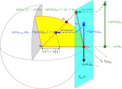
Figure 1: The proxy step-size technique. In the KKT system (15b), given $t$, the essence of the non-smooth equation (15b) is to decide a proper Lagrange multiplier $\mu$ that lands the point $\mathrm{prox}_{th}\left(\left(1-\mu t\right)\boldsymbol{x}_{k}-t\mathrm{grad}\,g|_{\boldsymbol{x}_{k}}\right)$ into the tangent plane at $\boldsymbol{x}_{k}$. Such a process is difficult as it is hard to solve equation (15b) for advanced $h(\cdot)$. Instead, we propose to use the proxy step-size $t^{\prime}$ to generate valid solutions to the KKT system (15b). In specific, we first move in the tangent plane at $\boldsymbol{x}_{k}$ by $-t^{\prime}\mathrm{grad}\,g|_{\boldsymbol{x}_{k}}$, and then apply the proximal to reach the point $\boldsymbol{z}=\mathrm{prox}_{\left|t^{\prime}\right|h}\left(\boldsymbol{x}_{k}-t^{\prime}\mathrm{grad}\,g|_{\boldsymbol{x}_{k}}\right)$. We see the point $\mathrm{prox}_{th}\left(\left(1-\mu t\right)\boldsymbol{x}_{k}-t\mathrm{grad}\,g|_{\boldsymbol{x}_{k}}\right)$ is the intersection of the line $(\boldsymbol{0},\boldsymbol{z})$ and the tangent plane at $\boldsymbol{x}_{k}$, given as $\frac{1}{\boldsymbol{x}_{k}^{\mathsf{T}}\boldsymbol{z}}\boldsymbol{z}$.

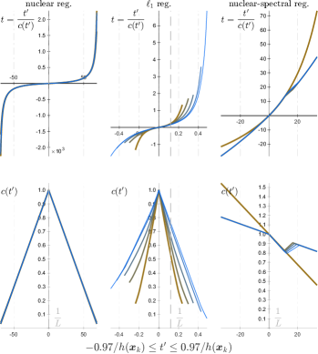
Figure 2: Numerical examples for Proposition 2 and Theorem 1. If $h(\cdot)$ is convex and absolutely homogeneous, then for $\left|t^{\prime}\right|<{1}/{h(\boldsymbol{x}_{k})}$, we have $c(t^{\prime})=\boldsymbol{x}_{k}^{\mathsf{T}}\boldsymbol{z}>0$ and thus the mapping $t=\phi(t^{\prime})={t^{\prime}}/c(t^{\prime})$ is monotonically increasing within this interval. The reference proxy step-size $1/L$ to be described in Section 4.4.1 is plotted as vertical dashed lines. These examples are obtained from the first $5$ iterations of: 1) fundamental matrix estimation with nuclear norm regularization, 2) correspondence association with $\ell_{1}$ norm regularization, and 3) self-calibration with nuclear-spectral norm regularization to be presented in Section 6.

4.2 The Mapping between Proxy Step-size and Actual Step-size

We denote $t=\phi(t^{\prime})={t^{\prime}}/{c(t^{\prime})}$ the mapping between $t^{\prime}$ and $t$ defined by equation (17b), where we introduce $c(t^{\prime})=\boldsymbol{x}_{k}^{\mathsf{T}}\boldsymbol{z}=\boldsymbol{x}_{k}^{\mathsf{T}}\mathrm{prox}_{\left|t^{\prime}\right|h}\left(\boldsymbol{x}_{k}-t^{\prime}\mathrm{grad}\,g|_{\boldsymbol{x}_{k}}\right)$.

Lemma 4.

Given arbitrary $t^{\prime}_{1}\neq 0$, $t^{\prime}_{2}\neq 0$, $t^{\prime}_{1}\neq t^{\prime}_{2}$, it can be shown that:

$$\epsilon(t^{\prime}_{1},t^{\prime}_{2})=\left(\frac{1}{\phi(t^{\prime}_{1})}-\frac{1}{\phi(t^{\prime}_{2})}\right)\left(\frac{1}{t^{\prime}_{1}}-\frac{1}{t^{\prime}_{2}}\right)\geq 0,$$ (19)

which means $1/{\phi(t^{\prime})}$ is monotonically increasing with respect to ${1}/{t^{\prime}}$.

Proof.

See Appendix D. ∎

Lemma 4 states the monotonicity between $1/t^{\prime}$ and $1/t$. To establish the monotonicity between $t^{\prime}$ and $t$ explicitly, it suffices to identify an interval where $c(t^{\prime})>0$.

Proposition 1.

If $c(t^{\prime})>0$ for $t^{\prime}\in[l,u]$, then $\phi(t^{\prime})$ is monotonically increasing with respect to $t^{\prime}$ for $t^{\prime}\in[l,u]$.

Proof.

Note that $\phi(t^{\prime})={t^{\prime}}/{c(t^{\prime})}$. We thus have:

$$t^{\prime}_{1}t^{\prime}_{2}\phi(t^{\prime}_{1})\phi(t^{\prime}_{2})=(t^{\prime}_{1}t^{\prime}_{2})^{2}/(c(t^{\prime}_{1})c(t^{\prime}_{2}))>0\Leftrightarrow c(t^{\prime}_{1})c(t^{\prime}_{2})>0$$

Therefore if $c(t^{\prime}_{1})c(t^{\prime}_{2})>0$, inequality (19) is equivalent to:

$$\left(\phi(t^{\prime}_{1})-\phi(t^{\prime}_{2})\right)\left(t^{\prime}_{1}-t^{\prime}_{2}\right)\geq 0.$$ (20)

We see $c(t^{\prime})>0$ is sufficient for $c(t^{\prime}_{1})c(t^{\prime}_{2})>0$. ∎

Now we characterize an interval in which $c(t^{\prime})>0$. For this purpose, we first prove the following global inequality for convex and absolutely homogeneous $h(\cdot)$:

Lemma 5.

Let $h(\cdot)$ be convex and absolutely homogeneous. Then for any $t$, $\boldsymbol{x}$ and $\boldsymbol{w}$, we have:

$$\langle\boldsymbol{w}-\mathrm{prox}_{\left|t\right|h}\left(\boldsymbol{w}\right),\,\boldsymbol{x}\rangle\leq\left|t\right|h(\boldsymbol{x}).$$ (21)

The inequality is tight for $\boldsymbol{x}=\mathrm{prox}_{\left|t\right|h}\left(\boldsymbol{w}\right)$.

Proof.

See Appendix E. ∎

Proposition 2.

If $h(\cdot)$ is convex and absolutely homogeneous, then $c(t^{\prime})\geq 1-\left|t^{\prime}\right|h(\boldsymbol{x}_{k})$.

Proof.

In Lemma 5, we set $\boldsymbol{w}=\boldsymbol{x}_{k}-t^{\prime}\mathrm{grad}\,g|_{\boldsymbol{x}_{k}}$ and $\boldsymbol{x}=\boldsymbol{x}_{k}$, which yields:

$$\langle\boldsymbol{x}_{k}-t^{\prime}\mathrm{grad}\,g|_{\boldsymbol{x}_{k}}-\mathrm{prox}_{\left|t^{\prime}\right|h}\left(\boldsymbol{x}_{k}-t^{\prime}\mathrm{grad}\,g|_{\boldsymbol{x}_{k}}\right),\,\boldsymbol{x}_{k}\rangle\\ \leq\left|t^{\prime}\right|h(\boldsymbol{x}_{k}).$$ (22)

We reorganize inequality (22) to complete the proof:

$$c(t^{\prime})=\boldsymbol{x}_{k}^{\mathsf{T}}\mathrm{prox}_{\left|t^{\prime}\right|h}\left(\boldsymbol{x}_{k}-t^{\prime}\mathrm{grad}\,g|_{\boldsymbol{x}_{k}}\right)\geq 1-\left|t^{\prime}\right|h(\boldsymbol{x}_{k}),$$

where we use $\langle\boldsymbol{x}_{k},\boldsymbol{x}_{k}\rangle=1$ and $\langle\mathrm{grad}\,g|_{\boldsymbol{x}_{k}},\boldsymbol{x}_{k}\rangle=0$. ∎

Theorem 1.

If $h(\cdot)$ is convex and absolutely homogeneous, then the mapping $t=\phi(t^{\prime})$ from proxy step-size $t^{\prime}$ to actual step-size $t$ is monotonically increasing for $\left|t^{\prime}\right|<{1}/{h(\boldsymbol{x}_{k})}$, and $\phi(0)=0$.

Proof.

By Proposition 2, we see $c(t^{\prime})>0$ for $\left|t^{\prime}\right|<{1}/{h(\boldsymbol{x}_{k})}$. Then by Proposition 1, $\phi(t^{\prime})$ is monotonically increasing with respect to $t^{\prime}$ for $\left|t^{\prime}\right|<{1}/{h(\boldsymbol{x}_{k})}$. By definition of the proximal operator in equation (3), we observe:

$$\lim_{t^{\prime}\rightarrow 0}\mathrm{prox}_{\left|t^{\prime}\right|h}\left(\boldsymbol{x}_{k}-t^{\prime}\mathrm{grad}\,g|_{\boldsymbol{x}_{k}}\right)=\boldsymbol{x}_{k},$$ (23)

from which we conclude $c(0)=1$, thus $\phi(0)=0$. ∎

Numerical examples to these results are given in Fig. 2. In practice, we require $t>0$, thus we use $0<t^{\prime}<{1}/{h(\boldsymbol{x}_{k})}$. Theorem 1 suggests that we can control the step-size $t$ by the proxy step-size $t^{\prime}$ within this interval.

Proposition 3.

If $h(\cdot)$ is convex and absolutely homogeneous and if $\left\|\mathrm{grad}\,g|_{\boldsymbol{x}_{k}}\right\|_{2}$ is bounded, then for any $t^{\prime}\neq 0$, we have $t=\phi(t^{\prime})\neq 0$.

Proof.

It can be shown (see Appendix F for details) that:

$$|t|\geq\frac{1}{\sqrt{\left(1/t^{\prime}\right)^{2}+\left\|\mathrm{grad}\,g|_{\boldsymbol{x}_{k}}\right\|_{2}^{2}}}.$$

Thus if $\left\|\mathrm{grad}\,g|_{\boldsymbol{x}_{k}}\right\|_{2}$ is bounded, then $t\neq 0$ for $t^{\prime}\neq 0$. ∎

We notice that $\left\|\mathrm{grad}\,g|_{\boldsymbol{x}_{k}}\right\|_{2}\leq\left\|\boldsymbol{I}-\boldsymbol{x}_{k}\boldsymbol{x}_{k}^{\mathsf{T}}\right\|\left\|\nabla g|_{\boldsymbol{x}_{k}}\right\|_{2}=\left\|\nabla g|_{\boldsymbol{x}_{k}}\right\|_{2}$, thus it suffices to have a bounded $\left\|\nabla g|_{\boldsymbol{x}_{k}}\right\|_{2}$. In particular, if the Euclidean gradient $\nabla g$ is Lipschitz continuous on the sphere, $\left\|\nabla g|_{\boldsymbol{x}_{k}}\right\|_{2}$ is bounded.

4.3 Line-search and Convergence

To establish the convergence proof, we make the following mild assumption on the cost $g(\cdot)$.

Assumption 1.

We assume the pullback function $g\left(\mathcal{R}_{\boldsymbol{x}}\left(\boldsymbol{v}\right)\right)$ with $\boldsymbol{v}\in\mathcal{T}_{\boldsymbol{x}}\mathcal{S}$ satisfies:

$$g\left(\mathcal{R}_{\boldsymbol{x}}\left(\boldsymbol{v}\right)\right)\leq g(\boldsymbol{x})+\langle\mathrm{grad}\,g(\boldsymbol{x}),\boldsymbol{v}\rangle+\frac{L}{2}\langle\boldsymbol{v},\boldsymbol{v}\rangle,$$ (24)

for a (known or unknown) constant $L>0$.

Assumption 1 holds if the ambient Euclidean space function $g(\cdot)$ on $\mathbb{R}^{n}$ has Lipschitz continuous gradient $\nabla g$ within the convex hull of $\mathcal{S}$ (Lemma 3 in [42]), i.e., within the unit ball $\{\boldsymbol{x}:\|\boldsymbol{x}\|_{2}\leq 1\}$. In other words, this assumption is satisfied if $g(\cdot)$ is not changing radically within the ball (like going to infinity at some point). Thus in practice, this assumption is hardly violated.

Based on Assumption 1, we propose the following line-search.

Line-search criterion. Search for a proxy step-size $t^{\prime}$, such that the actual step-size $t$ and the tangent update $\boldsymbol{v}_{k}$ solved from equation (18) satisfy:

$$g\left(\mathcal{R}_{\boldsymbol{x}_{k}}\left(\boldsymbol{v}_{k}\right)\right)\leq g(\boldsymbol{x}_{k})+\langle\mathrm{grad}\,g|_{\boldsymbol{x}_{k}},\boldsymbol{v}_{k}\rangle+\frac{1}{2t}\langle\boldsymbol{v}_{k},\boldsymbol{v}_{k}\rangle.$$ (25)

By Assumption 1, the inequality (25) is satisfied for any $0\leq t\leq 1/L$. This line-search criterion is in the same spirit as the one used in the classical Euclidean proximal gradient literature, where the Euclidean gradient $\nabla g|_{\boldsymbol{x}_{k}}$ is used instead of the Riemannian gradient here.

Line-search process. We start with an initial proxy step-size $t^{\prime}<1/h(\boldsymbol{x}_{k})$ and reduce $t^{\prime}$ until $t=\phi(t^{\prime})$ satisfies $0\leq t\leq 1/L$. This process is well-defined by the monotonicity of $t=\phi(t^{\prime})$, as proved by Theorem 1. One line-search iteration is given in Algorithm 1.

1

2

3

4function $(\boldsymbol{v}_{k},\,t,\,t^{\prime})\leftarrow$ lineSearch $(\boldsymbol{x}_{k},\,t^{\prime}_{\max})$

5      

6      $t^{\prime}\leftarrow\min\left\{t^{\prime}_{\max},{1}/{h(\boldsymbol{x}_{k})}\right\}$

7      

8      $\boldsymbol{z}\leftarrow\mathrm{prox}_{\left|t^{\prime}\right|h}\left(\boldsymbol{x}_{k}-t^{\prime}\mathrm{grad}\,g|_{\boldsymbol{x}_{k}}\right)$

9      $\boldsymbol{v}_{k}\leftarrow\frac{1}{\boldsymbol{x}_{k}^{\mathsf{T}}\boldsymbol{z}}\boldsymbol{z}-\boldsymbol{x}_{k}$

10      $t\leftarrow\frac{1}{\boldsymbol{x}_{k}^{\mathsf{T}}\boldsymbol{z}}t^{\prime}$

11      $Q_{L}=g(\boldsymbol{x}_{k})+\langle\mathrm{grad}\,g|_{\boldsymbol{x}_{k}},\boldsymbol{v}_{k}\rangle+\frac{1}{2t}\langle\boldsymbol{v}_{k},\boldsymbol{v}_{k}\rangle$

12      if $g\left(\mathcal{R}_{\boldsymbol{x}_{k}}\left(\boldsymbol{v}_{k}\right)\right)\leq Q_{L}$ then  return $(\boldsymbol{v}_{k},\,t,\,t^{\prime})$

13       else  $t^{\prime}\leftarrow 0.8t^{\prime}$, goto step $3$

14      

15 end

Algorithm 1 One line-search iteration.

We now show the line-search criterion guarantees a descent for the total cost $f\left(\boldsymbol{x}\right)=g\left(\boldsymbol{x}\right)+h\left(\boldsymbol{x}\right)$ at each iteration. See the PGS curve in Fig. 4 for an illustration.

Lemma 6.

For retraction (12), if $h(\cdot)$ is absolutely homogeneous and $\boldsymbol{v}_{k}\in\mathcal{T}_{\boldsymbol{x}_{k}}\mathcal{S}$, we have $h\left(\mathcal{R}_{\boldsymbol{x}_{k}}\left(\boldsymbol{v}_{k}\right)\right)\leq h\left(\boldsymbol{x}_{k}+\boldsymbol{v}_{k}\right)$.

Proof.

See Appendix G. ∎

Theorem 2.

Let $f\left(\boldsymbol{x}\right)=g\left(\boldsymbol{x}\right)+h\left(\boldsymbol{x}\right)$. If the line-search criterion (25) holds then:

$$f(\boldsymbol{x}_{k+1})=f\left(\mathcal{R}_{\boldsymbol{x}_{k}}\left(\boldsymbol{v}_{k}\right)\right)\leq f(\boldsymbol{x}_{k})-\frac{1}{2t}\langle\boldsymbol{v}_{k},\boldsymbol{v}_{k}\rangle.$$ (26)

Proof.

The first-order necessary optimality condition of problem (13) states that:

$$\boldsymbol{0}\in\mathrm{grad}\,g|_{\boldsymbol{x}_{k}}+\frac{1}{t}\boldsymbol{v}_{k}+\mathrm{proj}_{\mathcal{T}_{\boldsymbol{x}_{k}}\mathcal{S}}\,\partial h|_{\boldsymbol{x}_{k}+\boldsymbol{v}_{k}}$$ (27)

$$\Leftrightarrow -\mathrm{grad}\,g|_{\boldsymbol{x}_{k}}-\frac{1}{t}\boldsymbol{v}_{k}\in\mathrm{proj}_{\mathcal{T}_{\boldsymbol{x}_{k}}\mathcal{S}}\,\partial h|_{\boldsymbol{x}_{k}+\boldsymbol{v}_{k}}.$$ (28)

Because $\boldsymbol{v}_{k}\in\mathcal{T}_{\boldsymbol{x}_{k}}\mathcal{S}$ then $\langle\boldsymbol{z},\,\boldsymbol{v}_{k}\rangle=\langle\mathrm{proj}_{\mathcal{T}_{\boldsymbol{x}_{k}}\mathcal{S}}\boldsymbol{z},\,\boldsymbol{v}_{k}\rangle$ for any $\boldsymbol{z}\in\mathbb{R}^{n}$. By the convexity of $h\left(\cdot\right)$ at $\boldsymbol{x}_{k}+\boldsymbol{v}_{k}$, we obtain:

$$h\left(\boldsymbol{x}_{k}+\boldsymbol{v}_{k}\right) \leq h\left(\boldsymbol{x}_{k}\right)+\langle\partial h|_{\boldsymbol{x}_{k}+\boldsymbol{v}_{k}},\,\boldsymbol{v}_{k}\rangle$$ (29)

$$=h\left(\boldsymbol{x}_{k}\right)+\langle\mathrm{proj}_{\mathcal{T}_{\boldsymbol{x}_{k}}\mathcal{S}}\,\partial h|_{\boldsymbol{x}_{k}+\boldsymbol{v}_{k}},\,\boldsymbol{v}_{k}\rangle$$ (30)

$$\stackrel{{\scriptstyle(\ref{eq: the optimality condition of each iteration - reorganized})}}{{=}}h\left(\boldsymbol{x}_{k}\right)+\langle-\mathrm{grad}\,g|_{\boldsymbol{x}_{k}}-\frac{1}{t}\boldsymbol{v}_{k},\,\boldsymbol{v}_{k}\rangle.$$ (31)

By considering Lemma 6, we have the following inequality:

$$h\left(\mathcal{R}_{\boldsymbol{x}_{k}}\left(\boldsymbol{v}_{k}\right)\right)\leq h\left(\boldsymbol{x}_{k}\right)+\langle-\mathrm{grad}\,g|_{\boldsymbol{x}_{k}}-\frac{1}{t}\boldsymbol{v}_{k},\,\boldsymbol{v}_{k}\rangle.$$ (32)

Summing together inequalities (25) and (32), we obtain inequality (26). ∎

We denote $t^{\prime}_{k}$ $(k=0,1,\dots,K-1)$ to be the proxy step-size satisfying the line-search criterion (25) at iteration $k$. In the line-search process, we have:

$$0<t^{\prime}_{k}\leq\min\left\{t^{\prime}_{\max},{c}/{h(\boldsymbol{x}_{k})}\right\},\quad\mathrm{with\ }0<c<1.$$

We further denote the corresponding actual step-sizes as $t_{k}$ where $t_{k}=\phi(t^{\prime}_{k})=t^{\prime}_{k}/c(t^{\prime}_{k})$. From Theorem 1, we know $t_{k}\geq 0$. By Proposition 3, we know if $t^{\prime}_{k}\neq 0$ then $t_{k}\neq 0$ as $\left\|\mathrm{grad}\,g|_{\boldsymbol{x}_{k}}\right\|_{2}$ is bounded by the assumption of Lipschitz continuous gradient $\nabla g$ within the unit ball. Therefore we conclude $t_{k}>0$. To summarize, we have:

$$0<t_{\min}\leq t_{k}\leq t_{\max},$$

where we denote $t_{\min}=\min\{t_{k}\}$, $t_{\max}=\max\{t_{k}\}$.

At last, we show the iterations guided by the line-search process converge to a critical point of problem (2).

Proposition 4.

Assume $f(\boldsymbol{x})$ is bounded from below on $\mathcal{S}$, i.e., the problem is well-posed. If $g(\cdot)$ has Lipschitz continuous gradient $\nabla g$ within the unit ball $\{\boldsymbol{x}:\|\boldsymbol{x}\|\leq 1\}$, the line-search iterations converge to a critical point of problem (2).

Proof.

Let $f^{\star}$ be the optimal value, i.e., $f^{\star}\leq f(\boldsymbol{x})$ for any $\boldsymbol{x}$ on $\mathcal{S}$. Given $K$ iterations, inequality (26) implies:

$$f(\boldsymbol{x}_{0})-f^{\star} \geq f(\boldsymbol{x}_{0})-f({\boldsymbol{x}_{K}})=\sum_{k=0}^{K-1}\left(f(\boldsymbol{x}_{k})-f({\boldsymbol{x}_{k+1}})\right)$$

$$\geq\sum_{k=0}^{K-1}\frac{1}{2t_{k}}\langle\boldsymbol{v}_{k},\boldsymbol{v}_{k}\rangle=\sum_{k=0}^{K-1}\frac{t_{k}}{2}\langle\boldsymbol{v}_{k}/{t_{k}},\boldsymbol{v}_{k}/{t_{k}}\rangle.$$

Considering $0<t_{\min}\leq t_{k}\leq t_{\max}$, we have:

$$f(\boldsymbol{x}_{0})-f^{\star}\geq\frac{1}{2t_{\max}}\sum_{k=0}^{K-1}\left\|\boldsymbol{v}_{k}\right\|_{2}^{2},$$

$$f(\boldsymbol{x}_{0})-f^{\star}\geq\frac{t_{\min}}{2}\sum_{k=0}^{K-1}\left\|\boldsymbol{v}_{k}/{t_{k}}\right\|_{2}^{2}.$$

Denote $\epsilon_{0}=f(\boldsymbol{x}_{0})-f^{\star}$. Taking $K$ to the infinity, we obtain:

$$\lim_{K\rightarrow\infty}\,\sum_{k=0}^{K-1}\left\|\boldsymbol{v}_{k}\right\|_{2}^{2}\leq 2\epsilon_{0}t_{\max},\quad\lim_{K\rightarrow\infty}\,\sum_{k=0}^{K-1}\left\|\frac{\boldsymbol{v}_{k}}{t_{k}}\right\|_{2}^{2}\leq\frac{2\epsilon_{0}}{t_{\min}}.$$

Since $f(\boldsymbol{x})$ is bounded from below on $\mathcal{S}$, $\epsilon_{0}$ is a non-negative constant. Thus the right side of each inequality is bounded. Noting the left side is the summation of an infinite non-negative sequence, we have $\lim_{k\rightarrow\infty}\,\left\|\boldsymbol{v}_{k}\right\|_{2}=0$, $\lim_{k\rightarrow\infty}\,\left\|\boldsymbol{v}_{k}/{t_{k}}\right\|_{2}=0$, which means $\lim_{k\rightarrow\infty}\,\boldsymbol{v}_{k}=\boldsymbol{0}$, $\lim_{k\rightarrow\infty}\,\boldsymbol{v}_{k}/{t_{k}}=\boldsymbol{0}$. Lastly, we notice if $\boldsymbol{v}_{k}=\boldsymbol{0}$ and $\boldsymbol{v}_{k}/{t_{k}}=\boldsymbol{0}$, the first-order necessary optimality condition of problem (13), i.e., equation (27), becomes:

$$\boldsymbol{0}\in\mathrm{grad}\,g|_{\boldsymbol{x}_{k}}+\mathrm{proj}_{\mathcal{T}_{\boldsymbol{x}_{k}}\mathcal{S}}\,\partial h|_{\boldsymbol{x}_{k}},$$ (33)

which is exactly the first-order necessary optimality condition of problem (2) [29, 43]. ∎

Both $\left\|\boldsymbol{v}_{k}\right\|$ and $\left\|\boldsymbol{v}_{k}/{t_{k}}\right\|$ have linear convergence rates:

$$\min_{k=1,2,\dots,K}\left\|\boldsymbol{v}_{k}\right\|_{2}^{2}\leq\frac{2\epsilon_{0}t_{\max}}{K},\quad\min_{k=1,2,\dots,K}\left\|\frac{\boldsymbol{v}_{k}}{t_{k}}\right\|_{2}^{2}\leq\frac{\epsilon_{0}}{t_{\min}K},$$

with the constant decided by line-search strategies.

4.4 Algorithm

The final algorithm is to repeat the line-search until convergence. The pseudocode is provided in Algorithm 3, which unifies the PGS method in this section and the accelerated methods (A-PGS, AM-PGS) to be discussed shortly. Here we give additional components to complete the PGS method, before moving to its accelerated versions.

4.4.1 Maximum proxy step-size $t^{\prime}_{\max}$

While the constant $L$ in Assumption 1 (i.e., inequality (24)) exists ubiquitously, it is often not clear how to obtain $L$ in closed-form except for certain types of $g(\cdot)$ e.g., $g(\boldsymbol{x})=\boldsymbol{x}^{\mathsf{T}}\boldsymbol{A}\boldsymbol{x}$ where $L=2\sigma_{\max}(\boldsymbol{A})$ (see Section 6.1). Importantly, the existence of $L$ is used to establish proofs, but its actual value is never required to be known explicitly. Instead, to complete Algorithm 1, we need to decide $t^{\prime}_{\max}$.

Setting $t^{\prime}_{\max}$ from known $L$. In line-search criterion (25), $L$ establishes a lower-bound for the search, where if step-size $t<1/L$ then the total cost is guaranteed to descend (Theorem 2). While we work with proxy step-size $t^{\prime}$ and control step-size $t$ by $t=\phi(t^{\prime})$ in its monotone region, the value $1/L$ provides a good reference for the maximum proxy step-size $t^{\prime}_{\max}$. Practically, if $L$ is known ahead, we recommend using $t^{\prime}_{\max}=1/L$.

Setting $t^{\prime}_{\max}$ from line-search. Nonetheless, if $L$ is unknown (which is the usual case), $t^{\prime}_{\max}$ can be decided effectively from line-search. Such a line-search process is described in Algorithm 2, which is well-defined owing to the existence of $L$. Numerical examples are provided in Fig. 3. We compare the searched $t^{\prime}_{\max}$ and the known reference proxy step-size $t^{\prime}=1/L$ using their ratio, and see that a proper $t^{\prime}_{\max}$ close to $1/L$ can be found cheaply within $5$ - $10$ iterations.

1

2

3

4function $t^{\prime}_{\max}\leftarrow$ searchMaxProxyStepsize $(\boldsymbol{x}_{0})$

5      

6      $found\leftarrow false$, $ub\leftarrow{0.7}/{h(\boldsymbol{x}_{0})}$, $t^{\prime}\leftarrow ub$

7      

8      $\boldsymbol{z}\leftarrow\mathrm{prox}_{\left|t^{\prime}\right|h}\left(\boldsymbol{x}_{0}-t^{\prime}\mathrm{grad}\,g|_{\boldsymbol{x}_{0}}\right)$

9      $\boldsymbol{v}_{0}\leftarrow\frac{1}{\boldsymbol{x}_{0}^{\mathsf{T}}\boldsymbol{z}}\boldsymbol{z}-\boldsymbol{x}_{0}$

10      $t\leftarrow\frac{1}{\boldsymbol{x}_{0}^{\mathsf{T}}\boldsymbol{z}}t^{\prime}$

11      $Q_{L}=g(\boldsymbol{x}_{0})+\langle\mathrm{grad}\,g|_{\boldsymbol{x}_{0}},\boldsymbol{v}_{0}\rangle+\frac{1}{2t}\langle\boldsymbol{v}_{0},\boldsymbol{v}_{0}\rangle$

12      if $g\left(\mathcal{R}_{\boldsymbol{x}_{0}}\left(\boldsymbol{v}_{0}\right)\right)\leq Q_{L}$ then

13             if $t^{\prime}=ub$ then  return $t^{\prime}_{\max}\leftarrow ub$

14            

15            $found\leftarrow true$, $t^{\prime}\leftarrow\min\left\{2t^{\prime},ub\right\}$, goto step $3$

16       else if $found=true$ then  return $t^{\prime}_{\max}\leftarrow 0.5t^{\prime}$

17       else  $t^{\prime}\leftarrow 0.1t^{\prime}$, goto step $3$

18      

19 end

Algorithm 2 Search for proxy step-size $t^{\prime}_{\max}$.

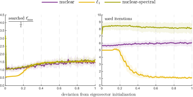
Figure 3: Examples of line-searched maximum proxy step-size $t^{\prime}_{\max}$, using different initializations $\boldsymbol{x}_{0}$ (detailed in Section 7.1.1). On the left we report the ratio $t^{\prime}_{\max}/(1/L)$, and on the right the used iterations.

Adaptive maximum proxy step-size $t^{\prime}_{\max}$. We observe that typically the corresponding $t=\phi(t^{\prime})=t^{\prime}/c(t^{\prime})$ is slightly larger than $t^{\prime}$ for $t^{\prime}$ around $1/L$, as $c(t^{\prime})$ is slightly below $1$ as seen in Fig. 2. Thus setting $t^{\prime}=1/L$ does not necessarily guarantee a line-search success from criterion (25) established on $t$. On the other hand, criterion (25) can also be satisfied for some $t$ greater than $1/L$. This motivates us to use an adaptive $t^{\prime}_{\max}$, where we set $t^{\prime}_{\max}$ to the working $t^{\prime}$ obtained at the previous iteration. This choice is controlled by the AdaptiveMaxProxyStepsize flag in Algorithm 3. We shall see such a strategy is useful to reduce subsequent total line-search iterations if $t^{\prime}_{\max}$ is initially obtained from the line-search in Algorithm 2 (see results in Fig. 5).

4.4.2 Stop criteria for convergence

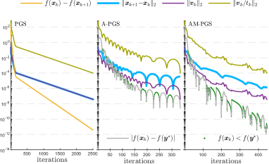
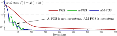
Figure 4: The convergence behavior of the PGS, A-PGS and AM-PGS methods. The example is drawn from self-calibration with nuclear norm regularization. For each method, we report the convergence of the estimate as $\left\|\boldsymbol{x}_{k+1}-\boldsymbol{x}_{k}\right\|_{2}$, of the tangent vector as $\|\boldsymbol{v}_{k}\|_{2}$ and of the first-order optimality as $\|\boldsymbol{v}_{k}/t_{k}\|_{2}$. The progression of the total cost $f(\boldsymbol{x}_{k})$ for each method is plotted in the second figure. In the first figure, for PGS, we report the convergence of the total cost as $f(\boldsymbol{x}_{k})-f(\boldsymbol{x}_{k+1})$ which is always positive from Theorem 2. For A-PGS and AM-PGS, we report the absolute value $|f(\boldsymbol{x}_{k})-f(\boldsymbol{y}^{\star})|$ and mark down cases where $f(\boldsymbol{x}_{k})<f(\boldsymbol{y}^{\star})$.

In general, we propose to monitor at least $\|\boldsymbol{v}_{k}\|_{2}$ and $\|\boldsymbol{v}_{k}/t_{k}\|_{2}$ as the stop criteria for convergence. Numerical examples are provided in Fig. 4. While other options are also possible, e.g., by monitoring $f(\cdot)$, these two indicators are important for the following reasons.

Convergence of estimates. The convergence of the estimates can be determined from the distance of $\boldsymbol{x}_{k}$ and $\boldsymbol{x}_{k+1}$, e.g., by using the chordal distance $d=\left\|\boldsymbol{x}_{k+1}-\boldsymbol{x}_{k}\right\|_{2}$ or the angle $\theta=\mathrm{acos}\left(\boldsymbol{x}_{k+1}^{\mathsf{T}}\boldsymbol{x}_{k}\right)$. Here we propose to check the length of the tangent vector $\|\boldsymbol{v}_{k}\|_{2}$. In fact, $\boldsymbol{v}_{k}=\mathcal{R}_{\boldsymbol{x}_{k}}^{-1}\left(\boldsymbol{x}_{k+1}\right)$ with $\mathcal{R}_{\cdot}^{-1}(\cdot)$ to be defined in equation (36), thus measuring the distance of $\boldsymbol{x}_{k}$ and $\boldsymbol{x}_{k-1}$.

Optimality as critical points. If $\boldsymbol{v}_{k}/{t_{k}}=\boldsymbol{0}$ and $\boldsymbol{v}_{k}=\boldsymbol{0}$, equation (27) becomes equation (33), thus $\boldsymbol{x}_{k}$ admits a critical point of problem (2) by satisfying the first-order optimality condition. For a deeper understanding, we see from the KKT system (17b):

$$\frac{\boldsymbol{v}_{k}}{t_{k}} =\frac{1}{t_{k}^{\prime}}(\boldsymbol{I}-\boldsymbol{x}_{k}\boldsymbol{x}_{k}^{\mathsf{T}})\,\mathrm{prox}_{\left|t_{k}^{\prime}\right|h}\left(\boldsymbol{x}_{k}-t_{k}^{\prime}\mathrm{grad}\,g|_{\boldsymbol{x}_{k}}\right)$$

$$=\mathrm{proj}_{\mathcal{T}_{\boldsymbol{x}_{k}}\mathcal{S}}\,\mathrm{prox}_{h}(\frac{1}{t_{k}^{\prime}}\boldsymbol{x}_{k}-\mathrm{grad}\,g|_{\boldsymbol{x}_{k}}).$$

Thus $\boldsymbol{v}_{k}/t_{k}$ is to project the proximal of $\frac{1}{t_{k}^{\prime}}\boldsymbol{x}_{k}-\mathrm{grad}\,g|_{\boldsymbol{x}_{k}}$ into the tangent space at $\boldsymbol{x}_{k}$. A critical point is where this tangent projection goes to zero.

4.4.3 Initialization $\boldsymbol{x}_{0}$

Typically, it is a good idea to initialize the regularized problem (2) from the solution of the original problem (1). However this choice is problem dependent and should be discussed specifically according to the problem at hand. For example, we initialize the regularized problems for fundamental matrix estimation and correspondence association with the solution of the Rayleigh quotient optimization (the original problem of these instances). However, for self-calibration, the regularized problems are initialized from the canonical DAQ after quasi-calibration, as the solution space of the original problem is likely to be ambiguous due to the critical motion sequence. Details are given in Section 6, and numerical validations provided in Section 7.1.

5 Acceleration using the Nesterov Momentum Technique

The conventional PGS method evaluates the gradient and proximal at the current estimate $\boldsymbol{x}_{k}$.

For the Nesterov momentum technique, the gradient and the proximal are instead evaluated at an auxiliary state $\boldsymbol{y}_{k}$ defined as a linear combination of the current estimate $\boldsymbol{x}_{k}$ and the previous estimate $\boldsymbol{x}_{k-1}$ [33, 14, 12]. In the Euclidean case, one accelerated iteration is defined as:

$$\begin{cases}\boldsymbol{x}_{k+1}=\boldsymbol{y}_{k}+\boldsymbol{v}_{k}\\[5.0pt] \boldsymbol{y}_{k+1}=\boldsymbol{x}_{k+1}+\frac{1-\alpha_{k}}{\alpha_{k+1}}\left(\boldsymbol{x}_{k}-\boldsymbol{x}_{k+1}\right),\quad\boldsymbol{y}_{0}=\boldsymbol{x}_{0},\end{cases}$$ (34)

where $\boldsymbol{v}_{k}$ is obtained by evaluating iteration (6) at $\boldsymbol{y}_{k}$ as:

$$\boldsymbol{v}_{k}=\operatorname*{\arg\min}_{\boldsymbol{v}\,\in\,\mathbb{R}^{n}}\ \langle\nabla g|_{\boldsymbol{y}_{k}},\boldsymbol{v}\rangle+\frac{1}{2t}\langle\boldsymbol{v},\boldsymbol{v}\rangle+h(\boldsymbol{y}_{k}+\boldsymbol{v}),$$

and the scalar sequence $\alpha_{k}$ $(k=1,2,\dots)$ is defined as:

$$\alpha_{k+1}=\frac{1+\sqrt{1+4\alpha_{k}^{2}}}{2},\quad\alpha_{0}=1.$$ (35)

The iteration defined above was first proposed by Nesterov for smooth optimization [33], and later extended to non-smooth composite optimization in [14, 12]. The original proof shows that the accelerated iteration attains quadratic convergence for convex cost functions. These results are also valid if the cost function is locally convex around a local minimum. Although Riemannian manifolds are typically non-convex, it has been shown that the Nesterov sequence can attain quadratic convergence rate for geodesically convex optimization problems on the manifold [44, 45].

To extend the above result to the sphere manifold, we need to evaluate the difference between $\boldsymbol{x}_{k+1}$ and $\boldsymbol{x}_{k}$ on the sphere. Inspired by [40], we define this difference as a vector $\Delta\boldsymbol{v}$ in the tangent space of $\boldsymbol{x}_{k+1}$, thus the first summation can be extended by the retraction at $\boldsymbol{x}_{k+1}$. Such $\Delta\boldsymbol{v}$ must satisfy $\mathcal{R}_{\boldsymbol{x}_{k+1}}(\Delta\boldsymbol{v})=\boldsymbol{x}_{k}$. Abusing notations, we define the inverse of the retraction, $\Delta\boldsymbol{v}=\mathcal{R}_{\boldsymbol{x}_{k+1}}^{-1}\left(\boldsymbol{x}_{k}\right)$, which can be calculated in closed-form as:

$$\mathcal{R}_{\boldsymbol{x}_{k+1}}^{-1}\left(\boldsymbol{x}_{k}\right)\stackrel{{\scriptstyle\text{def}}}{{=}}\frac{1}{\boldsymbol{x}_{k}^{\mathsf{T}}\boldsymbol{x}_{k+1}}\boldsymbol{x}_{k}-\boldsymbol{x}_{k+1}.$$ (36)

It can be easily verified that $\mathcal{R}_{\boldsymbol{x}_{k+1}}(\mathcal{R}_{\boldsymbol{x}_{k+1}}^{-1}(\boldsymbol{x}_{k}))=\boldsymbol{x}_{k}$ and $\mathcal{R}_{\boldsymbol{x}_{k+1}}^{-1}(\boldsymbol{x}_{k})\in\mathcal{T}_{\boldsymbol{x}_{x+1}}\mathcal{S}$ for any $\boldsymbol{x}_{k},\,\boldsymbol{x}_{k+1}\in\mathcal{S}$.

Overall we extend the Nesterov sequence to the sphere manifold as:

$$\begin{cases}\boldsymbol{x}_{k+1}=\mathcal{R}_{\boldsymbol{y}_{k}}\left(\boldsymbol{v}_{k}\right)\\[5.0pt] \boldsymbol{y}_{k+1}=\mathcal{R}_{\boldsymbol{x}_{k+1}}\left(\frac{1-\alpha_{k}}{\alpha_{k+1}}\mathcal{R}_{\boldsymbol{x}_{k+1}}^{-1}\left(\boldsymbol{x}_{k}\right)\right),\quad\boldsymbol{y}_{0}=\boldsymbol{x}_{0}.\end{cases}$$ (37)

The extension is to replace Euclidean addition and subtraction with Riemannian retraction $\mathcal{R}_{\cdot}(\cdot)$ and its inverse $\mathcal{R}^{-1}_{\cdot}(\cdot)$. Here $\boldsymbol{x}_{k}$ is obtained by evaluating iteration (13) at $\boldsymbol{y}_{k}$ as:

$$\boldsymbol{v}_{k}=\operatorname*{\arg\min}_{\boldsymbol{v}\,\in\,\mathcal{T}_{\boldsymbol{y}_{k}}\mathcal{S}}\ \langle\mathrm{grad}\,g|_{\boldsymbol{y}_{k}},\boldsymbol{v}\rangle+\frac{1}{2t}\langle\boldsymbol{v},\boldsymbol{v}\rangle+h(\boldsymbol{y}_{k}+\boldsymbol{v}),$$

and the scalar $\alpha_{k}$ is defined as in equation (35). The tangent update $\boldsymbol{v}_{k}$ can be solved in closed-form using the proxy step-size technique proposed in Section 4.

The estimates $\boldsymbol{x}_{k}$ $(k=1,2,\dots)$ generated from equation (37) do not guarantee the monotonicity of the total cost $f(\boldsymbol{x}_{k})=g(\boldsymbol{x}_{k})+h(\boldsymbol{x}_{k})$ [46]. On the manifold setting, this can sometimes lead to divergence if $\boldsymbol{v}_{k}$ is computed based on the SSNM method [40]. To detect and recover from potential failures, the authors in [40] introduced a safeguard by monitoring the progression of the cost function within several iterations. One potential reason for the divergence is the inexact computation of each iteration [46]:

“In our case, where the denoising subproblems are not solved exactly, monotonicity becomes an important issue. It might happen that due to the inexact computations of the denoising subproblems, the algorithm might become extremely non-monotone and in fact can even diverge!”

Practically in our experiments to be presented in Section 7, we did not observe the divergence of iterations by using the proxy step-size to obtain the tangent update $\boldsymbol{v}_{k}$. This may be due to the fact that we solve each iteration exactly (in closed-form) while the SSNM method used in [29, 40, 30] is iterative thus incurring inexact solutions.

Nonetheless, we propose a monotone algorithm for the sphere manifold based on Beck et al.’s [46] Euclidean version which has been proved to retain the quadratic convergence rate. Beck et al.’s [46] monotone algorithm is defined as:

$$\begin{cases}\boldsymbol{y}^{\star}=\boldsymbol{y}_{k}+\boldsymbol{v}_{k}\\[5.0pt] \boldsymbol{x}_{k+1}=\begin{cases}\boldsymbol{y}^{\star}&\quad\mathrm{if\ }f\left(\boldsymbol{y}^{\star}\right)<f(\boldsymbol{x}_{k})\\ \boldsymbol{x}_{k}&\quad\mathrm{otherwise}\end{cases}\\[15.0pt] \boldsymbol{y}_{k+1}=\begin{cases}\boldsymbol{y}^{\star}+\frac{1-\alpha_{k}}{\alpha_{k+1}}\left(\boldsymbol{x}_{k}-\boldsymbol{y}^{\star}\right)&\quad\mathrm{if\ }f\left(\boldsymbol{y}^{\star}\right)<f(\boldsymbol{x}_{k})\\ \boldsymbol{x}_{k}+\frac{\alpha_{k}}{\alpha_{k+1}}\left(\boldsymbol{y}^{\star}-\boldsymbol{x}_{k}\right)&\quad\mathrm{otherwise}.\\ \end{cases}\end{cases}$$

The above iteration ensures the monotonicity of the total cost $f(\cdot)$ by leveraging between the new estimate $\boldsymbol{y}^{\star}$ and the previous estimate $\boldsymbol{x}_{k}$. We extend Beck et al.’s monotone algorithm to the sphere manifold as follow:

$$\begin{cases}\boldsymbol{y}^{\star}=\mathcal{R}_{\boldsymbol{y}_{k}}\left(\boldsymbol{v}_{k}\right)\\[5.0pt] \boldsymbol{x}_{k+1}=\begin{cases}\boldsymbol{y}^{\star}&\quad\mathrm{if\ }f\left(\boldsymbol{y}^{\star}\right)<f(\boldsymbol{x}_{k})\\ \boldsymbol{x}_{k}&\quad\mathrm{otherwise}\end{cases}\\[15.0pt] \boldsymbol{y}_{k+1}=\begin{cases}\mathcal{R}_{\boldsymbol{y}^{\star}}\left(\frac{1-\alpha_{k}}{\alpha_{k+1}}\mathcal{R}^{-1}_{\boldsymbol{y}^{\star}}\left(\boldsymbol{x}_{k}\right)\right)&\quad\mathrm{if\ }f\left(\boldsymbol{y}^{\star}\right)<f(\boldsymbol{x}_{k})\\[5.0pt] \mathcal{R}_{\boldsymbol{x}_{k}}\left(\frac{\alpha_{k}}{\alpha_{k+1}}\mathcal{R}^{-1}_{\boldsymbol{x}_{k}}\left(\boldsymbol{y}^{\star}\right)\right)&\quad\mathrm{otherwise}.\end{cases}\end{cases}$$

The accelerated PGS (A-PGS), i.e., Nesterov sequence, and the accelerated monotone PGS (AM-PGS), i.e., Beck’s sequence, are implemented as pseudocode in Algorithm 3. An illustration of the convergence is given in Fig. 4.

1

2

3

4

input : method = PGS or A-PGS or AM-PGS

5

input : $\boldsymbol{x}_{0}$

6

7if known Lipschitz constant $L$ then  $t^{\prime}_{\max}\leftarrow 1/L$

8 else  $t^{\prime}_{\max}\leftarrow$ searchMaxProxyStepsize $(\boldsymbol{x}_{0})$

9

10$\boldsymbol{y}_{0}\leftarrow\boldsymbol{x}_{0}$, $\alpha_{0}\leftarrow 1$, $k\leftarrow 0$

11

12while  $k<maxIterations$  do

13      

14      $(\boldsymbol{v}_{k},\,t,\,t^{\prime})\leftarrow$ lineSearch $(\boldsymbol{y}_{k},\,t^{\prime}_{\max})$

15      

16      $\boldsymbol{y}^{\star}\leftarrow\mathcal{R}_{\boldsymbol{y}_{k}}\left(\boldsymbol{v}_{k}\right)$

17      

18      if AdaptiveMaxProxyStepsize then  $t^{\prime}_{\max}\leftarrow t^{\prime}$

19      

20      if method = PGS then

21             $\boldsymbol{x}_{k+1}\leftarrow\boldsymbol{y}^{\star}$

22             $\boldsymbol{y}_{k+1}\leftarrow\boldsymbol{y}^{\star}$

23       else if method = A-PGS or AM-PGS then

24             $\alpha_{k+1}\leftarrow\frac{1+\sqrt{1+4\alpha_{k}^{2}}}{2}$

25             $\boldsymbol{x}_{k+1}\leftarrow\boldsymbol{y}^{\star}$

26             $\boldsymbol{y}_{k+1}\leftarrow\mathcal{R}_{\boldsymbol{y}^{\star}}\left(\frac{1-\alpha_{k}}{\alpha_{k+1}}\mathcal{R}_{\boldsymbol{y}^{\star}}^{-1}\left(\boldsymbol{x}_{k}\right)\right)$

27            

28            if method = AM-PGS then

29                   if $g(\boldsymbol{y}^{\star})+h(\boldsymbol{y}^{\star})>g(\boldsymbol{x}_{k})+h(\boldsymbol{x}_{k})$ then

30                         $\boldsymbol{x}_{k+1}\leftarrow\boldsymbol{x}_{k}$

31                         $\boldsymbol{y}_{k+1}\leftarrow\mathcal{R}_{\boldsymbol{x}_{k}}\left(\frac{\alpha_{k}}{\alpha_{k+1}}\mathcal{R}_{\boldsymbol{x}_{k}}^{-1}\left(\boldsymbol{y}^{\star}\right)\right)$

32                        

33                   end if

34                  

35             end if

36            

37       end if

38      

39      if  $\|\boldsymbol{v}_{k}\|_{2}<1e-5$ and $\|\boldsymbol{v}_{k}/t\|_{2}<1e-3$  then

40             return $\boldsymbol{x}_{k+1}$

41       else  $k\leftarrow k+1$

42      

43 end while

44

Algorithm 3 A unified implementation of the PGS, A-PGS and AM-PGS methods.

6 Applications

6.1 Rayleigh Quotient Optimization

We consider $g(\boldsymbol{x})=\boldsymbol{x}^{\mathsf{T}}\boldsymbol{A}\boldsymbol{x}$ with $\boldsymbol{A}$ being a symmetric matrix. The Euclidean gradient at $\boldsymbol{x}\in\mathbb{R}^{n}$ is $\nabla g|_{\boldsymbol{x}}=2\boldsymbol{A}\boldsymbol{x}$. The Riemannian gradient at $x\in\mathcal{S}$ is:

$$\mathrm{grad}\,g(\boldsymbol{x})=\nabla g|_{\boldsymbol{x}}-\left\langle\boldsymbol{x},\nabla g|_{\boldsymbol{x}}\right\rangle\boldsymbol{x}\\ =2\boldsymbol{A}\boldsymbol{x}-2\left\langle\boldsymbol{x},\boldsymbol{A}\boldsymbol{x}\right\rangle\boldsymbol{x}=2\boldsymbol{A}\boldsymbol{x}-2(\boldsymbol{x}^{\mathsf{T}}\boldsymbol{A}\boldsymbol{x})\boldsymbol{x}.$$ (38)

Using retraction (12), the Lipschitz-type constant of $g\left(\mathcal{R}_{\boldsymbol{x}}\left(\boldsymbol{v}\right)\right)$ is $L=2\sigma_{\max}(\boldsymbol{A})$ (see Appendix H) where $\sigma_{\max}(\boldsymbol{A})$ denotes the largest singular value of $\boldsymbol{A}$.

Minimizing $g(\boldsymbol{x})=\boldsymbol{x}^{\mathsf{T}}\boldsymbol{A}\boldsymbol{x}$ on the sphere manifold is called Rayleigh quotient optimization:

$$\boldsymbol{x}_{0}=\operatorname*{\arg\min}_{\boldsymbol{x}\,\in\,\mathbb{R}^{n}}\ \boldsymbol{x}^{\mathsf{T}}\boldsymbol{A}\boldsymbol{x}\qquad\mathrm{s.t.}\quad\left\|\boldsymbol{x}\right\|_{2}=1.$$ (39)

The solution to this problem is given in closed-form, which is the bottom eigenvector of $\boldsymbol{A}$ (i.e., the eigenvector associated with the smallest eigenvalue), which often gives as a good initialization for its regularized versions.

6.2 Fundamental Matrix Estimation

6.2.1 Problem Statement

The fundamental matrix is a key algebraic model of the two-view geometry [1, 3, 47]. We denote $\boldsymbol{p}_{i}\leftrightarrow{\boldsymbol{p}_{i}^{\prime}}$ $\left(i=\left[1:m\right]\right)$ the homogeneous coordinates of corresponding points in two images. In the noise-free case, the epipolar constraint holds as:

$${\boldsymbol{p}_{i}^{\prime}}^{\mathsf{T}}\boldsymbol{F}\boldsymbol{p}_{i}=0,\quad i=\left[1:m\right].$$ (40)

The matrix $\boldsymbol{F}\in\mathbb{R}^{3\times 3}$ is called the fundamental matrix, defined up to scale, thus we seek for $\boldsymbol{F}$ on the unit sphere such that $\left\|\boldsymbol{F}\right\|_{F}=1$. Importantly, $\mathrm{rank}(\boldsymbol{F})=2$ is required. A related concept is the essential matrix for normalized calibration, for which we refer to a recent work [48].

To estimate $\boldsymbol{F}$, we can formulate a cost function based on the algebraic error as:

$$\varphi(\boldsymbol{F}) =\frac{1}{m}\sum_{i=1}^{m}\left({\boldsymbol{p}_{i}^{\prime}}^{\mathsf{T}}\boldsymbol{F}\boldsymbol{p}_{i}\right)^{2}=\frac{1}{m}\sum_{i=1}^{m}\left(\left(\boldsymbol{p}_{i}^{\mathsf{T}}\otimes{\boldsymbol{p}_{i}^{\prime}}^{\mathsf{T}}\right)\mathrm{vec}\left(\boldsymbol{F}\right)\right)^{2}$$

$$=\frac{1}{m}\left\|\boldsymbol{H}\mathrm{vec}\left(\boldsymbol{{F}}\right)\right\|_{2}^{2},$$

where the $i$-th row of $\boldsymbol{H}$ is $\boldsymbol{p}_{i}^{\mathsf{T}}\otimes{\boldsymbol{p}_{i}^{\prime}}^{\mathsf{T}}$. We denote $\boldsymbol{x}=\mathrm{vec}\left(\boldsymbol{{F}}\right)$ and $\boldsymbol{F}=\mathrm{mat}\left(\boldsymbol{{x}}\right)$, where $\mathrm{vec}(\cdot)$ is the standard column-wise matrix vectorization and $\mathrm{mat}(\cdot)$ is its inverse operation. Defining $\boldsymbol{A}=\frac{1}{m}\boldsymbol{H}^{\mathsf{T}}\boldsymbol{H}$, we see the fundamental matrix problem is an instance of problem (39).

The solution $\boldsymbol{F}_{0}=\mathrm{mat}(\boldsymbol{x}_{0})$ solved from problem (39) is usually of rank $3$. A remedy is to subsequently round the solution $\boldsymbol{F}_{0}$ using the rank-$2$ approximation via the Singular Value Decomposition (SVD). This two-stage solution is the eight-point algorithm. Instead, we give a low-rank solution using the nuclear norm regularization.

6.2.2 Nuclear Norm Regularization

The nuclear norm of a matrix $\left\|\boldsymbol{X}\right\|_{\ast}$, defined as the summation of its singular values, is the tightest convex envelop of the rank function within the unit ball $\left\{\boldsymbol{X}\in\mathbb{R}^{m\times n}\,:\,\left\|\boldsymbol{X}\right\|_{2}\leq 1\right\}$ [9]. Nuclear norm regularization has been widely used as a technique to promote low-rank in Euclidean optimization problems [13], while a direct deployment to the manifold setting seems to be obscure with the results in [29, 32], mainly due to the challenge incurred in evaluating the generalized Jacobian matrix of a non-smooth function. In contrast, our technique can handle nuclear norm regularization with no effort. We apply nuclear norm regularization to problem (39) as:

$$\operatorname*{\arg\min}_{\boldsymbol{x}\,\in\,\mathbb{R}^{n}}\ \boldsymbol{x}^{\mathsf{T}}\boldsymbol{A}\boldsymbol{x}+\lambda\|\mathrm{mat}\left(\boldsymbol{x}\right)\|_{\ast}\quad\mathrm{s.t.}\quad\|\boldsymbol{x}\|_{2}=1,$$ (41)

where $\lambda\geq 0$ is a given constant controlling the strength of regularization.

In problem (41), the regularization term is $h\left(\boldsymbol{x}\right)=\lambda\left\|\mathrm{mat}\left(\boldsymbol{x}\right)\right\|_{\ast}$, which is convex but non-smooth. Besides, $h\left(\cdot\right)$ is absolutely homogeneous, i.e., $h\left(\alpha\boldsymbol{x}\right)=\left|\alpha\right|h\left(\boldsymbol{x}\right)$, because:

$$\lambda\left\|\mathrm{mat}\left(\alpha\boldsymbol{x}\right)\right\|_{\ast}=\lambda\left\|\alpha\mathrm{mat}\left(\boldsymbol{x}\right)\right\|_{\ast}=\lambda\left|\alpha\right|\left\|\mathrm{mat}\left(\boldsymbol{x}\right)\right\|_{\ast}.$$ (42)

The first equality holds because $\mathrm{mat}\left(\boldsymbol{x}\right)$ is a linear operator, and the second because norms are absolutely homogeneous.

Let $\boldsymbol{X}=\mathrm{mat}\left(\boldsymbol{x}\right)$ and denote its SVD as $\boldsymbol{X}=\boldsymbol{U}\boldsymbol{\Sigma}\boldsymbol{V}^{\mathsf{T}}$. For the nuclear norm function $\lambda\left\|\boldsymbol{X}\right\|_{\ast}$, the proximal is given in closed-form [49], where $\mathrm{prox}_{t\lambda\left\|\cdot\right\|_{\ast}}(\boldsymbol{X})=\boldsymbol{U}(\boldsymbol{\Sigma}-t\lambda\boldsymbol{I})_{+}\boldsymbol{V}^{\mathsf{T}}$. Here $\boldsymbol{A}_{+}\stackrel{{\scriptstyle\text{def}}}{{=}}\max\{\boldsymbol{A},\,\boldsymbol{0}\}$ proceeds element-wise. Thus we obtain the proximal of $h\left(\cdot\right)$ as:

$$\mathrm{prox}_{th}\left(\boldsymbol{x}\right)=\mathrm{vec}\left(\boldsymbol{U}\left(\boldsymbol{\Sigma}-t\lambda\boldsymbol{I}\right)_{+}\boldsymbol{V}^{\mathsf{T}}\right).$$ (43)

6.3 Correspondence Association

6.3.1 Problem Statement

The correspondence association problem using pairwise constraints can be formulated as a Rayleigh quotient optimization as well [5]. We denote the association hypothesis that a point $i$ in the point-cloud $\mathcal{Q}$ is matched with a point $i^{\prime}$ in the point-cloud $\mathcal{Q}^{\prime}$ as $\mathfrak{h}_{ii^{\prime}}$. The correspondence problem is to estimate the likelihood $p(\mathfrak{h}_{ii^{\prime}})$ $(i\in\mathcal{Q},\,i^{\prime}\in\mathcal{Q}^{\prime})$ of all possible association hypotheses, collected as components of the state vector $\boldsymbol{x}$.

To that end, we can design an adjacency matrix $\boldsymbol{M}$ from the pairwise consistency of hypotheses [5]. A common practice is based on the change of distance:

$$\boldsymbol{M}(\mathfrak{h}_{ii^{\prime}},\mathfrak{h}_{jj^{\prime}})=\begin{cases}4.5-\frac{(d_{ij}-d_{i^{\prime}j^{\prime}})^{2}}{2\delta_{d}^{2}}&\mathrm{if}\ \left|d_{ij}-d_{i^{\prime}j^{\prime}}\right|<3\delta_{d}\\ 0&\mathrm{otherwise},\end{cases}$$ (44)

where $d_{ij}$ is the Euclidean distance between the points $i$ and $j$ in $\mathcal{Q}$, $d_{i^{\prime}j^{\prime}}$ the distance between the points $i^{\prime}$ and $j^{\prime}$ in $\mathcal{Q}^{\prime}$, and $\delta_{d}$ a tuning parameter.

The resulting problem is formalized as maximizing the overall consistency $\boldsymbol{x}^{\mathsf{T}}\boldsymbol{M}\boldsymbol{x}$ on the unit sphere, as an instance of problem (39) by letting $\boldsymbol{A}=-\boldsymbol{M}$. The estimate of $\boldsymbol{x}$ is further used to decide the final correspondences, based on various assumptions, e.g., one point in $\mathcal{Q}$ can only be matched with one point in $\mathcal{Q}^{\prime}$ [5].

The match hypotheses solved this way are dense, while many of them present with contradictions or low probabilities. It is thus favorable to have a sparse $\boldsymbol{x}$, where some unlikely hypotheses and contradictions are pruned away. We give such a sparse solution by $\ell_{1}$ norm regularization.

6.3.2 $\ell_{1}$ Norm Regularization

It has been known that $\ell_{1}$ norm regularization can favor sparsity in Euclidean [12] and manifold optimization [29, 32]. We apply $\ell_{1}$ norm regularization to problem (39) as:

$$\operatorname*{\arg\min}_{\boldsymbol{x}\,\in\,\mathbb{R}^{n}}\ \boldsymbol{x}^{\mathsf{T}}\boldsymbol{A}\boldsymbol{x}+\lambda\|\boldsymbol{x}\|_{\ell_{1}}\quad\mathrm{s.t.}\quad\|\boldsymbol{x}\|_{2}=1,$$ (45)

where $\lambda\geq 0$ is a given constant controlling the strength of regularization. In this case, $h(\boldsymbol{x})=\lambda\|\boldsymbol{x}\|_{\ell_{1}}$, which is convex and absolutely homogeneous. The proximal of $h(\boldsymbol{x})$, often termed soft shrinkage operator, is given element-wise as:

$$\mathrm{prox}_{th}\left(\boldsymbol{x}\right)_{i}=\mathrm{sgn}(\boldsymbol{x}_{i})(\left|\boldsymbol{x}_{i}\right|-t\lambda)_{+}.$$ (46)

6.4 Camera Self-calibration

6.4.1 Problem Statement

In projective reconstruction, we obtain a set of projective cameras $\tilde{\boldsymbol{P}}_{i}\in\mathbb{R}^{3\times 4}$:

$$\tilde{\boldsymbol{P}}_{i}\propto\boldsymbol{P}_{i}\boldsymbol{H}^{-1}\quad(i\in\left[1:n\right]),$$ (47)

which differ from the Euclidean cameras $\boldsymbol{P}_{i}\in\mathbb{R}^{3\times 4}$ by a common projective transformation $\boldsymbol{H}\in\mathbb{R}^{4\times 4}$. The camera self-calibration problem is to infer $\boldsymbol{H}$ from $\tilde{\boldsymbol{P}}_{i}$ [3].

The key algebraic model to this task is the Dual Absolute Quadric (DAQ), a rank-$3$ symmetric matrix in $\mathbb{R}^{4\times 4}$ defined up to scale [2]. In specific, the DAQ in the Euclidean space, termed the canonical DAQ, takes the form $\Omega_{\infty}^{\ast}=\mathrm{diag}(1,1,1,0)$. We denote the DAQ in the projective space (where $\tilde{\boldsymbol{P}}_{i}$ is defined) by $\boldsymbol{Q}_{\infty}^{\ast}=\boldsymbol{H}\Omega_{\infty}^{\ast}\boldsymbol{H}^{\mathsf{T}}$. The image of the DAQ, denoted by $\omega_{i}^{\ast}$, is invariant under $\boldsymbol{H}$:

$$\omega_{i}^{\ast}\propto\tilde{\boldsymbol{P}}_{i}\boldsymbol{Q}_{\infty}^{\ast}\tilde{\boldsymbol{P}}_{i}^{\mathsf{T}}\propto\boldsymbol{P}_{i}\Omega_{\infty}^{\ast}\boldsymbol{P}_{i}^{\mathsf{T}}\propto\boldsymbol{K}_{i}\boldsymbol{K}_{i}^{\mathsf{T}},$$ (48)

where $\boldsymbol{K}_{i}\in\mathbb{R}^{3\times 3}$ is the intrinsic matrix of $\boldsymbol{P}_{i}$. At its core, the self-calibration problem is to estimate $\boldsymbol{Q}_{\infty}^{\ast}$ from equation (48) using various constraints on $\boldsymbol{K}_{i}$.

Here we consider a linear approach developed for cameras with varying focal lengths [50]. In this case, we have $\boldsymbol{K}_{i}\boldsymbol{K}_{i}^{\mathsf{T}}\propto\mathrm{diag}(f_{i}^{2},f_{i}^{2},1)$. Based on equation (48), we have:

$$\tilde{\boldsymbol{a}}_{i}^{\mathsf{T}}\boldsymbol{Q}_{\infty}^{\ast}\tilde{\boldsymbol{a}}_{i}=\tilde{\boldsymbol{b}}_{i}^{\mathsf{T}}\boldsymbol{Q}_{\infty}^{\ast}\tilde{\boldsymbol{b}}_{i}$$ (49a)

$$\tilde{\boldsymbol{a}}_{i}^{\mathsf{T}}\boldsymbol{Q}_{\infty}^{\ast}\tilde{\boldsymbol{b}}_{i}=0,\ \tilde{\boldsymbol{a}}_{i}^{\mathsf{T}}\boldsymbol{Q}_{\infty}^{\ast}\tilde{\boldsymbol{c}}_{i}=0,\ \tilde{\boldsymbol{b}}_{i}^{\mathsf{T}}\boldsymbol{Q}_{\infty}^{\ast}\tilde{\boldsymbol{c}}_{i}=0,$$ (49b)

where $\tilde{\boldsymbol{P}}_{i}^{\mathsf{T}}=\begin{bmatrix}\tilde{\boldsymbol{a}}_{i}&\tilde{\boldsymbol{b}}_{i}&\tilde{\boldsymbol{c}}_{i}\end{bmatrix}$. Equation (49b) is linear in $\boldsymbol{Q}_{\infty}^{\ast}$ thus can be rewritten as:

$$\boldsymbol{M}_{i}\,\mathrm{vec_{t}}\left(\boldsymbol{Q}_{\infty}^{\ast}\right)=\boldsymbol{M}_{i}\,\boldsymbol{x}=\boldsymbol{0},$$ (50)

where we have defined $\mathrm{vec_{t}}\left(\boldsymbol{Q}_{\infty}^{\ast}\right)=\boldsymbol{x}\in\mathbb{R}^{10}$ comprising of the upper triangular elements of $\boldsymbol{Q}_{\infty}^{\ast}$, and $\mathrm{mat_{t}}\left(\boldsymbol{x}\right)=\boldsymbol{Q}_{\infty}^{\ast}$ its inverse operation. Since $\boldsymbol{Q}_{\infty}^{\ast}$ is defined up to scale so is $\boldsymbol{x}$ and we minimize the cost $\varphi(\boldsymbol{x})=\frac{1}{n}\sum_{i=1}^{n}\left\|\boldsymbol{M}_{i}\,\boldsymbol{x}\right\|_{2}^{2}$ on the unit sphere. Upon defining $\boldsymbol{A}=\frac{1}{n}\sum_{i=1}^{n}\boldsymbol{M}_{i}^{\mathsf{T}}\boldsymbol{M}_{i}$, we see it is another instance of problem (39).

Just as the case of the fundamental matrix estimation, the DAQ estimated from solving problem (39) is typically of rank $4$ instead of rank $3$, thus an SVD based rounding process is used subsequently.

Once obtaining a rank-$3$ estimate of $\boldsymbol{Q}_{\infty}^{\ast}$, we can recover $\boldsymbol{H}$ up to a similarity transformation. This is usually done by the eigen decomposition of $\boldsymbol{Q}_{\infty}^{\ast}$. Let $\boldsymbol{Q}_{\infty}^{\ast}=\boldsymbol{U}\boldsymbol{\Lambda}\boldsymbol{U}^{\mathsf{T}}$, with $\boldsymbol{\Lambda}=\mathrm{diag}(\lambda_{1},\lambda_{2},\lambda_{3},0)$. We then set $\boldsymbol{H}\propto\boldsymbol{U}\,\mathrm{diag}(\sqrt{\lambda_{1}},\sqrt{\lambda_{2}},\sqrt{\lambda_{3}},1)$. The estimate of $\boldsymbol{H}$ determines camera $\boldsymbol{P}_{i}$, and $\boldsymbol{K}_{i}$ afterwards by decomposing $\boldsymbol{P}_{i}$.

6.4.2 Nuclear Norm Regularization

One issue regarding self-calibration is the critical motion sequences (CMS) [51]. The CMSs are camera configurations where self-calibration is ambiguous due to the lack of sufficient constraints. Among which, we consider the artificial CMS that can be resolved by enforcing the rank deficiency of the DAQ during the estimation rather than a posteriori. For the linear self-calibration described in equation (49b), one such CMS is that - all the cameras’ principal axes intersect at a fixed point, i.e., all the cameras look towards a common point. In this case, there only exist two rank deficient solutions [51]: one rank-$3$ solution (desired) and one rank-$1$ solution (undesired).

In analogy to the fundamental matrix estimation, we use nuclear norm regularization to promote low rank. This case is similar to what we have discussed in Section 6.2.2. We omit the details as they can be readily derived by replacing $\mathrm{mat}(\cdot)$ with $\mathrm{mat}_{t}(\cdot)$ and $\mathrm{vec}(\cdot)$ with $\mathrm{vec}_{t}(\cdot)$ in problem (41).

6.4.3 Nuclear-Spectral Norm Regularization

The aforementioned nuclear norm regularization resolves the CMS only partly due to the existence of the rank-$1$ solution. We propose to avoid the rank-$1$ solution by additionally including a spectral norm to penalize the largest singular value. The nuclear-spectral norm regularizer is:

$$h(\boldsymbol{x})=\lambda_{1}\|\mathrm{mat_{t}}\left(\boldsymbol{x}\right)\|_{\ast}+\lambda_{2}\|\mathrm{mat_{t}}\left(\boldsymbol{x}\right)\|_{2},$$ (51)

where $\lambda_{1}$ and $\lambda_{2}$ control the regularization strength of each part. We apply this regularizer to problem (39) as:

$$\operatorname*{\arg\min}_{\boldsymbol{x}\,\in\,\mathbb{R}^{n}} \boldsymbol{x}^{\mathsf{T}}\boldsymbol{A}\boldsymbol{x}+\lambda_{1}\|\mathrm{mat_{t}}\left(\boldsymbol{x}\right)\|_{\ast}+\lambda_{2}\|\mathrm{mat_{t}}\left(\boldsymbol{x}\right)\|_{2}$$ (52)

$$\mathrm{s.t.} \|\boldsymbol{x}\|_{2}=1.$$

Denote the SVD of $\mathrm{mat_{t}}\left(\boldsymbol{x}\right)$ as $\mathrm{mat_{t}}\left(\boldsymbol{x}\right)=\boldsymbol{U}\boldsymbol{\Sigma}\boldsymbol{V}^{\mathsf{T}}$. Since both the nuclear and spectral norm are orthogonal invariant, we can derive the proximal of $h(\cdot)$ in a similar manner as the derivation used for the nuclear norm. The proximal of $h(\cdot)$ in equation (51) is given as follow:

$$\mathrm{prox}_{th}\left(\boldsymbol{x}\right)=\mathrm{vec_{t}}\left(\boldsymbol{U}\left(\boldsymbol{\Sigma}-t\lambda_{1}\boldsymbol{I}-t\lambda_{2}\boldsymbol{E}_{1}\right)_{+}\boldsymbol{V}^{\mathsf{T}}\right),$$ (53)

where $\boldsymbol{E}_{1}=\mathrm{diag}(1,0,\cdots,0)$ is a diagonal matrix where the top-left element is $1$ and the rests are all-zeros.

7 Experimental Results

7.1 The Proposed PGS Algorithm

We first provide an evaluation of the PGS methods, i.e., PGS, A-PGS and AM-PGS methods in Algorithm 3.

7.1.1 Experiment Setup

Numerical instances. We experiment with the Rayleigh quotient optimization, and draw numerical examples from different applications which essentially form different $\boldsymbol{A}$ matrices in problem (39):

• nuclear norm reg. — fundamental matrix estimation with nuclear norm regularization,

• $\ell_{1}$ norm reg. — correspondence association with $\ell_{1}$ norm regularization,

• nuclear-spectral norm reg. — self-calibration with nuclear-spectral norm regularization.

In this section, we distinguish these instances by the type of regularization used, i.e., nuclear, $\ell_{1}$ and nuclear-spectral.

Initialization. The numerical examples used in this section are special forms ot the Rayleigh quotient optimization problem (39), and its optimal solution is known to be the bottom eigenvector of matrix $\boldsymbol{A}$ which we denote by $\boldsymbol{\xi}_{\boldsymbol{A}}$. To examine the convergence behavior with respect to different initializations, we create a range of initial values $\boldsymbol{x}_{0}$ by adding independent zero-mean Gaussian noise element-wisely to $\boldsymbol{\xi}_{\boldsymbol{A}}$. For the $k$-th vector element, we let:

$$\boldsymbol{\xi}[k]\leftarrow\boldsymbol{\xi}_{\boldsymbol{A}}[k]+\epsilon,\quad\epsilon\sim\mathcal{N}(0,\delta_{\mathrm{init}}),$$ (54)

and normalize $\boldsymbol{\xi}$ to get the initial value $\boldsymbol{x}_{0}=\boldsymbol{\xi}/\|\boldsymbol{\xi}\|_{2}$. Intuitively, $\delta_{\mathrm{init}}$ controls the deviation from the eigenvector initialization $\boldsymbol{\xi}_{\boldsymbol{A}}$, and if $\delta_{\mathrm{init}}$ is large, the above process simulates random initialization.

Proxy step-size strategies. We examine the following proxy step-size strategies.

• LipschitzFixed — $t^{\prime}_{\max}=1/L$ initially, and $t^{\prime}_{\max}$ is kept fixed in the following iterations;

• LipschitzAdaptive — $t^{\prime}_{\max}=1/L$ initially, and at each iteration $t^{\prime}_{\max}$ is updated to the previous working proxy step-size $t^{\prime}$;

• SearchedFixed — $t^{\prime}_{\max}$ is obtained from Algorithm 2 initially, and $t^{\prime}_{\max}$ is kept fixed in the following iterations;

• SearchedAdaptive — $t^{\prime}_{\max}$ is obtained from Algorithm 2, and at each iteration $t^{\prime}_{\max}$ is updated to the previous working proxy step-size $t^{\prime}$.

7.1.2 Results

We report the results with a $20$ run Monte-Carlo simulation for each PGS method and each proxy step-size strategy with respect to different initializations.

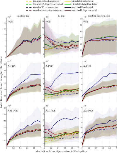
Figure 5: The convergence of the PGS, A-PGS and AM-PGS methods by using different proxy step-size strategies. Results are reported as the total line-search and the accepted iterations with respect to different initialization.

Convergence by used iterations. We examine the convergence by the used iterations in Fig. 5. In particular, we distinguish the total line-search iterations (the overall iterations processed in Algorithm 1) and the accepted iterations (the iterations used in Algorithm 3). The final verdicts is as follows: a) In general, we observe no significant differences for the accepted iterations across different proxy step-size strategies. b) However, the proxy step-size strategy SearchedFixed is not recommended, as it often leads to line-search failures especially when the initialization is bad, as reflected by the number of total line-search iterations. Therefore, if $t^{\prime}_{\max}$ is obtained from line-search in Algorithm 2, we recommend at each iteration updating $t^{\prime}_{\max}$ to the previous working proxy step-size $t^{\prime}$. c) If $t^{\prime}_{\max}$ is initialized as $1/L$ from the Lipschitz constant $L$, both strategies LipschitzFixed and LipschitzAdaptive give similar results. d) We observe accelerated methods A-PGS and AM-PGS converge much faster than the unaccelerated PGS method, thus are generally recommended.

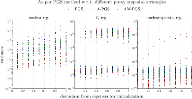
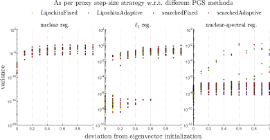
Figure 6: The variation of the optimal costs for each case.

Variation of the optimal costs. We compare the optimal costs of each Monte-Carlo run in Fig. 6. In specific, in the top figure, for each PGS method (i.e., PGS/A-PGS/AM-PGS), we compare the costs obtained from different proxy step-size strategies. Likewise, in the bottom figure, for each proxy step-size strategy, we compare the costs obtained from different PGS methods. The difference is evaluated as the variation of the optimal costs. From Fig. 6, we see that the optimal costs are mostly the same if $\delta_{\mathrm{init}}$ in equation (54) is small, or otherwise stated if the initialization $\boldsymbol{x}_{0}$ is close to the eigenvector initialization $\boldsymbol{\xi}_{\boldsymbol{A}}$ where we simulate good initializations. As $\delta_{\mathrm{init}}$ grows where we simulate bad initializations, the differences grow as different PGS methods and proxy step-size strategies can lead to the convergence to different local minima. This phenomenon is extremely clear for the $\ell_{1}$ norm regularized instances, where $\boldsymbol{x}$ is valued mostly below $0.5$ (see the example in Fig. 10) and $\delta_{\mathrm{init}}>0.5$ sets $\boldsymbol{x}_{0}$ almost to random.

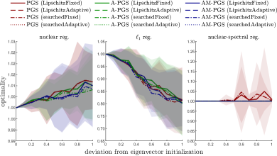
Figure 7: The impact of different initializations.

Optimality of the optimal costs. We evaluate the optimal cost obtained from the initialization $\boldsymbol{x}_{0}$ by comparing with the optimal cost obtained from the eigenvector initialization $\boldsymbol{\xi}_{\boldsymbol{A}}$. For each Monte-Carlo run, we define the optimality:

$$\mathrm{optimality}=\frac{\mathrm{optimal\ cost\ initialized\ from}\ \boldsymbol{x}_{0}}{\mathrm{optimal\ cost\ initialized\ from}\ \boldsymbol{\xi}_{\boldsymbol{A}}},$$

to benchmark the influence of different initializations. If the optimality metric is close to $1$, then the optimal cost is close to the one obtained from the eigenvector initialization, and otherwise if this metric deviates from $1$ then the computed solution is considered to be suboptimal. Intuitively, the optimality curve defines the robustness against bad initializations. The statistics for each tested case are plotted in Fig. 7. It is worth noting that the costs of the $\ell_{1}$ norm regularized instances are negative (as $\boldsymbol{A}=-\boldsymbol{M}$), thus the optimality metric is below $1$. For the problem instances used in this paper, the PGS, A-PGS and AM-PGS methods are in general robust to a large range of initializations, while the $\ell_{1}$ norm regularized instances are more sensitive to initializations.

7.2 Comparison with ManPG [29] and AManPG [40]

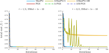
Figure 8: The convergence of ManPG and AManPG using the line-search criterion (16) in comparison to the proposed one.

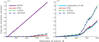
Figure 9: The computational time per iteration by using the SSNM method [32] (used in [29, 40, 30]) and the proposed proxy step-size technique (used in the PGS, A-PGS and AM-PGS methods). The matrix-vector multiplication $\boldsymbol{A}\boldsymbol{x}$ is computed by the level-2 BLAS routine “dsymv”.

We compare with the ManPG method [29] and its accelerated version AManPG [40]. Due to the difficulties of implementing the generalized Clarke differential for nuclear norm regularization, the comparison is only performed by applying $\ell_{1}$ regularization to problem (39). We use the C++ implementation of ManPG and AManPG released in [40]. AManPG uses a safeguard mechanism every $N$ iterations, where we set $N=5$ and $N=100$ and term the resulting methods as AManPG-5 and AManPG-100. The error-tolerance of the SSNM method [32] is set to $1e-10$.

We implemented our methods PGS, A-PGS, and AM-PGS in C++ as well for a fair comparison.

	$e_{dist}$ (pixels)$\downarrow$					$e_{rep}$ (pixels)$\downarrow$
	8pt	PGS5	PGS10	PGS	Gp	8pt	PGS5	PGS10	PGS	Gp
Chapel(0,1)	0.386	0.380	0.380	0.379	0.376	0.260	0.256	0.256	0.255	0.254
Keble(0,3)	0.248	0.247	0.247	0.247	0.247	0.175	0.175	0.175	0.175	0.175
Desktop(C,D)	0.574	0.336	0.303	0.288	0.268	0.406	0.238	0.214	0.204	0.190
Library(1,3)	0.428	0.409	0.405	0.405	0.400	0.302	0.289	0.286	0.286	0.282
Merton1(1,3)	0.308	0.295	0.291	0.288	0.277	0.217	0.209	0.205	0.203	0.196
Merton2(1,3)	0.596	0.528	0.498	0.472	0.404	0.421	0.373	0.352	0.334	0.286
Arch	0.304	0.299	0.299	0.299	0.298	0.215	0.211	0.211	0.211	0.211
Yard	0.433	0.429	0.429	0.428	0.426	0.306	0.303	0.303	0.302	0.301
Slate	0.246	0.184	0.177	0.170	0.163	0.129	0.097	0.093	0.089	0.085
Ben1	0.203	0.144	0.128	0.102	0.101	0.142	0.101	0.089	0.071	0.070
Ben2	0.139	0.086	0.063	0.050	0.048	0.097	0.060	0.044	0.035	0.033

TABLE I: Fundamental matrix estimation with nuclear norm regularization (with data in [52]).

7.2.1 Line-search Criteria and Convergence

Theoretical justification. In ManPG’s line-search criterion (16), we first need to assign $t$ and then perform line-search for $\alpha_{k}$ to ensure the descent of the total cost $f(\cdot)$. From Theorem 2 of our work, we see that if $t\leq 1/L$ with $L$ being the Lipschitz constant, it suffices to set $\alpha_{k}=1$ in the ManPG’s line-search criterion (16). The authors in [29, 40] assume known Lipschitz constant $L$ and suggest to use $t=1/L$ as a reference. Although for arbitrary $t>0$, the existence of $\alpha_{k}$ for criterion (16) is proved in [29], we observe a proper $t$ in ManPG/AManPG is required.

Numerical validation. On the left of Fig. 8, we see by setting $t=1/L$, ManPG’s line-search (16) works almost the same way as the proposed PGS line-search. On the right of Fig. 8, we run the same numerical instance again by setting $t=3/L$ in ManPG and AManPG. In this case, ManPG converges slower as seen from its curve being slightly shifted right. With some fluctuations, the accelerated method AManPG-5 manages to converge while the convergence is even slower than ManPG. AManPG-10 simply does not converge.

In practice, if the Lipschitz constant $L$ is unknown, it is expected that an approximated $L$ may cause a lot of trouble in ManPG’s line-search criterion (16) as used in [29, 40]. In the proposed line-search, this is never a problem. Intuitively, we fix $\alpha_{k}=1$ in criterion (16) and use proxy step-size $t^{\prime}$ to find a working $t$ from the line-search criterion (25). This process is well-defined by the Lipschitz type assumption (i.e., Assumption 1), and ensures the descent of the total cost $f(\cdot)$ by Theorem 2.

7.2.2 Computational Complexity

The proposed PGS methods are much faster than ManPG and AManPG. Both ManPG and AManPG rely on the SSNM method [32] to solve the non-smooth KKT system, thus we compare the computation time per iteration of the proposed proxy step-size technique with that of the SSNM method. We report the timing statistics per iteration in Fig. 9, with respect to the dimension of the $\boldsymbol{A}$ matrix in problem (39). It is clearly seen that the proposed proxy step-size technique is substantially faster than the SSNM method. An ablation study shows that the computation time per iteration of the PGS, A-PGS and AM-PGS methods is mostly decided by the matrix-vector multiplication $\boldsymbol{A}\boldsymbol{x}_{k}$ used in evaluating the Euclidean gradient $\nabla g|_{\boldsymbol{x}}=2\boldsymbol{A}\boldsymbol{x}_{k}$ and the cost function $g(\boldsymbol{x}_{k})=\boldsymbol{x}_{k}^{\mathsf{T}}\boldsymbol{A}\boldsymbol{x}_{k}$. The A-PGS and AM-PGS methods have the same per iteration complexity, while being twice more expensive than the PGS method due to an extra evaluation at the auxiliary state $\boldsymbol{y}_{k}$.

7.3 Fundamental Matrix Estimation

We find $\lambda=0.01$ works well in general, after normalizing the image points [3]. For this problem, we find that the PGS algorithm converges mostly within $20$ iterations. For most of the cases, $10$ iterations or even $5$ are sufficient to reduce the last singular value $\sigma_{3}$ close enough to zero. Therefore aside from the PGS method (with full convergence), aiming for an efficient engineering design, we propose the following two truncated PGS algorithms:

• PGS₅. $5$ PGS iterations, followed by a rank-$2$ rounding by setting $\sigma_{3}=0$.

• PGS₁₀. $10$ PGS iterations, followed by a rank-$2$ rounding by setting $\sigma_{3}=0$.

We use two benchmark algorithms: a) the normalized eight point algorithm (denoted as 8pt), b) the global polynomial optimization [52] (denoted as Gp) with a formulation based on $\det(\boldsymbol{F})=0$.

We run the 8pt, PGS₅, PGS₁₀, PGS and Gp methods on a list of standard benchmarks, and report in Table I a) $e_{dist}$ the distance between the epipolar line and the corresponding image feature point [53], and b) $e_{rep}$ the reprojection error of the triangulated 3D points. Overall, the $e_{dist}$ and $e_{rep}$ statistics decrease consistently over the 8pt, PGS₅, PGS₁₀, PGS, and Gp methods. Table I shows that the PGS₅ and PGS₁₀ methods, with a close performance towards the PGS method, consistently outperform the 8pt method, and they can give almost the same accuracy as the global method Gp.

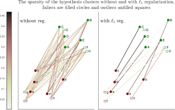
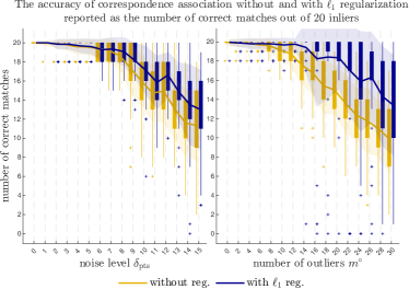
Figure 10: Correspondence association with $\ell_{1}$ norm regularization. With $\ell_{1}$ regularization, high probability hypotheses are enhanced while low probability hypotheses are trimmed off, resulting in a sparser and more consistent cluster of association hypotheses. Therefore the correct correspondences (i.e., inliers) can be identified more robustly.

7.4 Correspondence Association

The regularization strength is set as $\lambda=-\sigma_{\min}(\boldsymbol{A})/(\sqrt{n}-1)=\sigma_{\max}(\boldsymbol{M})/(\sqrt{n}-1)$ with $n$ the dimension of $\boldsymbol{A}$. This choice is motivated by the canonical basis vector $\boldsymbol{e}_{k}^{\mathsf{T}}$. Since the diagonal elements of $\boldsymbol{A}$ are zero by construction, the total cost at $\boldsymbol{e}_{k}$ is $f(\boldsymbol{e}_{k})=\boldsymbol{e}_{k}\boldsymbol{A}\boldsymbol{e}_{k}^{\mathsf{T}}+\lambda\|\boldsymbol{e}_{k}\|_{\ell_{1}}=\lambda$. Noting that $1\leq\|\boldsymbol{x}\|_{\ell_{1}}\leq\sqrt{n}$, we thus have the following relation:

$$f(\boldsymbol{x})<f(\boldsymbol{e}_{k}) \Leftrightarrow\boldsymbol{x}^{\mathsf{T}}\boldsymbol{A}\boldsymbol{x}+\lambda\|\boldsymbol{x}\|_{\ell_{1}}\leq\boldsymbol{x}^{\mathsf{T}}\boldsymbol{A}\boldsymbol{x}+\lambda\sqrt{n}<\lambda$$

$$\Leftrightarrow\lambda\leq-\frac{\boldsymbol{x}^{\mathsf{T}}\boldsymbol{A}\boldsymbol{x}}{\sqrt{n}-1}\leq-\frac{\sigma_{\min}(\boldsymbol{A})}{\sqrt{n}-1},$$

where the used $\lambda$ is chosen as the largest possible value.

Our experimental setup is similar to the one used in Section 5.1 of [5]. We simulate a 2-dimensional point-cloud $\mathcal{Q}$ of $m$ points, with $x-y$ coordinates uniformly distributed in $[0,\,256\sqrt{m/10}]$. Then we add zero-mean Gaussian noise with standard deviation $\delta_{\mathrm{pts}}$ to each point in $\mathcal{Q}$, and rotate and translate the whole $\mathcal{Q}$ to obtain $\mathcal{Q}^{\prime}$. We generate $m^{\circ}$ outliers in both $\mathcal{Q}$ and $\mathcal{Q}^{\prime}$ uniformly in the same region. We use $\delta_{d}=5$ in equation (44) as in [5].

The results are reported in Fig. 10. In the first figure, we give an illustration (using $m=5$) that with $\ell_{1}$ norm regularization, many unlikely hypotheses are trimmed off, thus yielding a sparse hypothesis cluster. In the second figure, we set $m=20$ and report the number of correct matches with respect to different noise levels and with respect to different outlier ratios. For each case, we use a $50$ run Monte-Carlo simulation. It is clear that the association accuracy is consistently improved by using $\ell_{1}$ norm regularization.

7.5 Linear Self-calibration

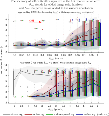
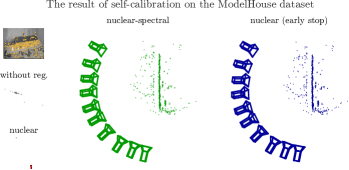
Figure 11: Self-calibration with the nuclear norm and the nuclear-spectral norm regularization. We show the results with the critical motion sequence (CMS) where the camera principal axes pass approximately through the geometric center of the observed object (case R4 of Table $1$ in [51]).

7.5.1 Implementation

We find normalization is essential to obtain stable self-calibration results. The key points of our implementation are sketched as follows:

1. Image point normalization. Let $(p_{x},p_{y})$ be the principal point of the camera. If this is unknown, we approximate $(p_{x},p_{y})=(I_{x}/2,I_{y}/2)$, where $I_{x}$ and $I_{y}$ are the width and height of the image. The average distance of all image points to $(p_{x},p_{y})$ is denoted by $s$. We normalize all image points by a common transformation $\boldsymbol{T}^{-1}$:

   $$\boldsymbol{T}=\begin{pmatrix}s&0&p_{x}\\ 0&s&p_{y}\\ 0&0&1\end{pmatrix},\ \boldsymbol{T}^{-1}=\begin{pmatrix}1/s&0&-{p_{x}}/{s}\\ 0&1/s&-{p_{y}}/{s}\\ 0&0&1\end{pmatrix}.$$

2. Projective reconstruction using projective bundle-adjustment from the normalized image points.

3. Quasi-Euclidean rectification [54]. We approximate the intrinsic matrix of each camera computed in step $2)$ as $\boldsymbol{K}_{i}=\mathrm{diag}(f_{i},f_{i},1)$, with $f_{i}=2\sqrt{m_{x}^{2}+m_{y}^{2}}$ where $m_{x}$ and $m_{y}$ are the maximum range in the $x$- and $y$- coordinates. Using this approximate $\boldsymbol{K}_{i}$, we compute an approximate estimate of $\boldsymbol{Q}_{\infty}^{\ast}$ from the DAQ constraint (48) i.e., $\tilde{\boldsymbol{P}}_{i}\boldsymbol{Q}_{\infty}^{\ast}\tilde{\boldsymbol{P}}_{i}^{\mathsf{T}}\propto\boldsymbol{K}_{i}\boldsymbol{K}_{i}^{\mathsf{T}}$, and rectify the projective reconstruction approximately.

4. Linear self-calibration from the quasi-Euclidean rectification in step $3)$. We initialize the PGS methods from the canonical DAQ $\Omega_{\infty}^{\ast}=\mathrm{diag}(1,1,1,0)$.

5. Transforming cameras $\boldsymbol{P}_{i}$ obtained from step $4)$ by $\boldsymbol{T}$. Lastly, $\boldsymbol{T}\boldsymbol{P}_{i}$ are the final estimate of Euclidean cameras.

We use $\lambda=0.01$ for the nuclear norm regularization, and $\lambda_{1}=0.01$, $\lambda_{2}=2\lambda_{1}$ for the nuclear-spectral norm regularization.

7.5.2 Simulated Data

We simulate a scene comprising: a) $50$ points spreading randomly in a diameter of $3$ meters; b) $7$ cameras circularly distributed $30$ meters away from the point-cloud. All cameras are oriented towards the centroid of the point-cloud, thus the simulated scenario is an artificial CMS whose ambiguity can be removed using the rank deficiency of the DAQ. We evaluate the performance of each method with respect to the perturbation of camera orientations $\delta_{\mathrm{cam}}$ and the noise of image points $\delta_{\mathrm{img}}$. We use the 3D reconstruction error as the evaluation metric, which is computed by the similarity Procrustes analysis between the ground-truth point-cloud and the estimated point-cloud.

We conduct two sets of experiments. First, we use the fixed image noise $\delta_{\mathrm{img}}=4$ pixels and decrease $\delta_{\mathrm{cam}}$ to gradually bring the camera configuration to the CMS. Second, we set the camera configuration to the exact CMS where $\delta_{\mathrm{cam}}=0$ and then test the performance with respect to different image noise $\delta_{\mathrm{img}}$. We report the reconstruction error with a $50$ run Monte-Carlo simulation in Fig. 11.

As shown in Fig. 11, when facing the CMS, the classical method without regularization fails, and the method with nuclear-spectral norm regularization is more robust than the one with nuclear norm regularization e.g., in case of the exact CMS where $\delta_{\mathrm{cam}}=0$ and $\delta_{\mathrm{img}}>3$. It is interesting to see that the nuclear-norm regularization works well for less noisy scenarios of the CMS, e.g., when $\delta_{\mathrm{img}}<2$. For these cases, it seems that the solution of the nuclear-norm regularized problem is well-trapped at the local minimum (the rank-$3$ DAQ), while the gradient is not large enough to go to the global minimum (the rank-$1$ DAQ). To examine this hypothesis, we use an early-stop trick (by setting the maximum PGS iterations to $1000$) in the nuclear norm regularization, and observe that with the early-stop trick the nuclear-norm regularized method mostly performs well.

7.5.3 Real Data

A qualitative example of the CMS is given in Fig. 11 using a real dataset called ModelHouse where all cameras look towards the geometric center of a model house. In this scenario, matrix $\boldsymbol{A}$ has two eigenvalues close to zero. The classic method fails because the solution space is ambiguous. The nuclear norm regularized method fails by converging to the rank-$1$ solution. The nuclear-spectral norm regularized method can find the correct rank-$3$ solution thus recover the correct Euclidean geometry. The nuclear norm regularized method with the early stop trick also works. Intuitively, the spectral norm in the nuclear-spectral norm regularization prevents the algorithm from gliding to the rank-$1$ solution, and the early stop trick has the similar functionality.

8 Conclusion

We have proposed the proxy step-size technique, and presented an effective solution to problem (2) for convex and absolutely homogeneous $h(\cdot)$. The proposed solution is: exact (satisfying the first-order necessary optimality condition), elegant (simple and in closed-form), and easily applicable (to nuclear norm regularization etc.). Future work includes extending the proxy-step size technique to the oblique and the Stiefel manifolds, and analyzing the convergence rate of the accelerated methods in Algorithm 3.

Fang Bai Fang Bai was born in Ningxia Province, China, in 1988. He received the B.Sc. degree in computer science and technology from Nankai University, China, in 2010, and the Ph.D. degree in robotics from University of Technology Sydney, Australia, in 2020. His research has been focused on mathematical abstractions in robotics and computer vision. He has conducted several fundamental breakthroughs on related topics as the first-author, e.g., the cycle based pose graph optimization, the equation to predict the change of optimal values, and the closed-form solution for template-free deformable Procrustes analysis.

Adrien Bartoli Adrien Bartoli has held the position of Professor of Computer Science at Université Clermont Auvergne since fall 2009 and has been a member of Institut Universitaire de France since 2016. He is currently on leave as research scientist at the University Hospital of Clermont-Ferrand and as Chief Scientific Officer at SurgAR. He leads the Endoscopy and Computer Vision (EnCoV) research group at the University and Hospital of Clermont-Ferrand. His main research interests are in computer vision, including image registration and Shape-from-X for deformable environments, and their application to computer-aided medical interventions.

Appendix A Properties of proximal

A.1 Convexity

If $h(\cdot)$ is convex, then for any $\boldsymbol{x}$ and $\boldsymbol{x}_{0}$, we have:

$$h(\boldsymbol{x})\geq h(\boldsymbol{x}_{0})+\langle\partial{h}|_{\boldsymbol{x}_{0}},\,\boldsymbol{x}-\boldsymbol{x}_{0}\rangle.$$

A.2 Firm non-expansiveness and non-expansiveness

For a convex $h(\cdot)$, let $\boldsymbol{z}_{1}=\mathrm{prox}_{th}\left(\boldsymbol{w}_{1}\right)$ and $\boldsymbol{z}_{2}=\mathrm{prox}_{th}\left(\boldsymbol{w}_{2}\right)$ with $t\geq 0$. Then the following holds:

• Firm non-expansiveness:

  $$\left\|\boldsymbol{z}_{1}-\boldsymbol{z}_{2}\right\|_{2}^{2}\leq\langle\boldsymbol{z}_{1}-\boldsymbol{z}_{2},\,\boldsymbol{w}_{1}-\boldsymbol{w}_{2}\rangle;$$ (55)

• Non-expansiveness:

  $$\left\|\boldsymbol{z}_{1}-\boldsymbol{z}_{2}\right\|_{2}^{2}\leq\left\|\boldsymbol{w}_{1}-\boldsymbol{w}_{2}\right\|_{2}^{2}.$$ (56)

Proof.

The solution of the proximal is characterized by its first-order necessary condition:

$$\boldsymbol{0}\in\partial{h}|_{\boldsymbol{z}_{1}}+\frac{1}{t}(\boldsymbol{z}_{1}-\boldsymbol{w}_{1})\Leftrightarrow\frac{1}{t}(\boldsymbol{w}_{1}-\boldsymbol{z}_{1})\in\partial{h}|_{\boldsymbol{z}_{1}},$$ (57)

$$\boldsymbol{0}\in\partial{h}|_{\boldsymbol{z}_{2}}+\frac{1}{t}(\boldsymbol{z}_{2}-\boldsymbol{w}_{2})\Leftrightarrow\frac{1}{t}(\boldsymbol{w}_{2}-\boldsymbol{z}_{2})\in\partial{h}|_{\boldsymbol{z}_{2}}.$$ (58)

By the convexity of $h(\cdot)$, we have:

$$h(\boldsymbol{z}_{1})\geq h(\boldsymbol{z}_{2})+\langle\partial{h}|_{\boldsymbol{z}_{2}},\,\boldsymbol{z}_{1}-\boldsymbol{z}_{2}\rangle$$ (59a)

$$h(\boldsymbol{z}_{2})\geq h(\boldsymbol{z}_{1})+\langle\partial{h}|_{\boldsymbol{z}_{1}},\,\boldsymbol{z}_{2}-\boldsymbol{z}_{1}\rangle.$$ (59b)

Substituting equations (57) and (58) into (59b), we have:

$$h(\boldsymbol{z}_{1})\geq h(\boldsymbol{z}_{2})+\langle\frac{1}{t}(\boldsymbol{w}_{2}-\boldsymbol{z}_{2}),\,\boldsymbol{z}_{1}-\boldsymbol{z}_{2}\rangle$$ (60a)

$$h(\boldsymbol{z}_{2})\geq h(\boldsymbol{z}_{1})+\langle\frac{1}{t}(\boldsymbol{w}_{1}-\boldsymbol{z}_{1}),\,\boldsymbol{z}_{2}-\boldsymbol{z}_{1}\rangle.$$ (60b)

Summing together inequalities (60a) and (60b), we have:

$$\langle\boldsymbol{w}_{2}-\boldsymbol{z}_{2}-\boldsymbol{w}_{1}+\boldsymbol{z}_{1},\,\boldsymbol{z}_{1}-\boldsymbol{z}_{2}\rangle\leq 0.$$

Expanding the above, we obtain the firm non-expansiveness (55). By the Cauchy–Schwarz inequality, we obtain:

$$\left|\langle\boldsymbol{z}_{1}-\boldsymbol{z}_{2},\,\boldsymbol{w}_{1}-\boldsymbol{w}_{2}\rangle\right|\leq\left\|\boldsymbol{z}_{1}-\boldsymbol{z}_{2}\right\|_{2}\left\|\boldsymbol{w}_{1}-\boldsymbol{w}_{2}\right\|_{2}.$$

After canceling $\left\|\boldsymbol{z}_{1}-\boldsymbol{z}_{2}\right\|_{2}$ in the firm non-expansiveness (55), we obtain non-expansiveness (56).

∎

A.3 Proof of Lemma 2

By definition of the proximal, we write:

$$\mathrm{prox}_{th}\left(\boldsymbol{0}\right)=\operatorname*{\arg\min}_{\boldsymbol{x}}\left\{th\left(\boldsymbol{x}\right)+\frac{1}{2}\left\|\boldsymbol{x}\right\|^{2}\right\},\quad t\geq 0$$ (61)

Since $h(\cdot)$ is convex and absolutely homogeneous, from Lemma 1, we have $h\left(\boldsymbol{x}\right)\geq 0$ and $h\left(\boldsymbol{0}\right)=0$. Thus, we observe that the optimal cost of problem (61) is $0$ which is attained at $\boldsymbol{x}=\boldsymbol{0}$ as $h\left(\boldsymbol{0}\right)=0$ and $\left\|\boldsymbol{x}\right\|=0$. This concludes $\mathrm{prox}_{th}\left(\boldsymbol{0}\right)=\boldsymbol{0}$ if $h(\cdot)$ is convex and absolutely homogeneous. The inequalities $\left\|\mathrm{prox}_{th}(\boldsymbol{w})\right\|_{2}^{2}\leq\langle\mathrm{prox}_{th}(\boldsymbol{w}),\,\boldsymbol{w}\rangle$ and $\left\|\mathrm{prox}_{th}(\boldsymbol{w})\right\|_{2}\leq\left\|\boldsymbol{w}\right\|_{2}$ follow from firm non-expansiveness (55) and non-expansiveness (56), by setting $\boldsymbol{w}_{1}=\boldsymbol{w}$ and $\boldsymbol{w}_{2}=\boldsymbol{0}$.

Appendix B Derivation of KKT System (15b)

We write $\boldsymbol{0}\in\partial\mathcal{L}_{\boldsymbol{v}_{k}}$ as follow:

$$\boldsymbol{0}\in\mathrm{grad}\,g|_{\boldsymbol{x}_{k}}+\frac{1}{t}\boldsymbol{v}_{k}+\partial h|_{\boldsymbol{x}_{k}+\boldsymbol{v}_{k}}+\mu\boldsymbol{x}_{k}$$

$$\Leftrightarrow\left(1-\mu t\right)\boldsymbol{x}_{k}-t\mathrm{grad}\,g|_{\boldsymbol{x}_{k}}\in t\partial h|_{\boldsymbol{x}_{k}+\boldsymbol{v}_{k}}+\boldsymbol{x}_{k}+\boldsymbol{v}_{k}$$

$$\Leftrightarrow\boldsymbol{x}_{k}+\boldsymbol{v}_{k}=\mathrm{prox}_{th}\left(\left(1-\mu t\right)\boldsymbol{x}_{k}-t\mathrm{grad}\,g|_{\boldsymbol{x}_{k}}\right).$$

Therefore:

$$\boldsymbol{v}_{k}=\mathrm{prox}_{th}\left(\left(1-\mu t\right)\boldsymbol{x}_{k}-t\mathrm{grad}\,g|_{\boldsymbol{x}_{k}}\right)-\boldsymbol{x}_{k},$$

which is equation (15a). Considering $\boldsymbol{x}_{k}^{\mathsf{T}}\boldsymbol{v}_{k}=0$ with equation (15a), we obtain equation (15b).

Appendix C Proof of Lemma 3

By definition of the proximal, we write:

$$\mathrm{prox}_{th}\left(\alpha\boldsymbol{w}\right)=\operatorname*{\arg\min}_{\boldsymbol{x}}\left\{h\left(\boldsymbol{x}\right)+\frac{1}{2t}\left\|\boldsymbol{x}-\alpha\boldsymbol{w}\right\|^{2}\right\}\stackrel{{\scriptstyle\text{def}}}{{=}}\boldsymbol{z}.$$

Since $h(\cdot)$ is absolutely homogeneous, $h\left(\boldsymbol{x}\right)=\left|\alpha\right|h\left(\frac{1}{\alpha}\boldsymbol{x}\right)$. The above equation can thus be written as:

$$\boldsymbol{z} =\operatorname*{\arg\min}_{\boldsymbol{x}}\left\{\left|\alpha\right|h\left(\frac{1}{\alpha}\boldsymbol{x}\right)+\frac{\alpha^{2}}{2t}\left\|\frac{1}{\alpha}\boldsymbol{x}-\boldsymbol{w}\right\|^{2}\right\}$$

$$=\operatorname*{\arg\min}_{\boldsymbol{x}}\left\{h\left(\frac{1}{\alpha}\boldsymbol{x}\right)+\frac{1}{2\frac{t}{\left|\alpha\right|}}\left\|\frac{1}{\alpha}\boldsymbol{x}-\boldsymbol{w}\right\|^{2}\right\}$$

$$\Leftrightarrow\frac{1}{\alpha}\boldsymbol{z}=\mathrm{prox}_{\frac{t}{\left|\alpha\right|}h}\left(\boldsymbol{w}\right).$$

Therefore $\boldsymbol{z}=\mathrm{prox}_{th}\left(\alpha\boldsymbol{w}\right)=\alpha\mathrm{prox}_{\frac{t}{\left|\alpha\right|}h}\left(\boldsymbol{w}\right)$.

Appendix D Proof of Lemma 4

From equation (17b), we obtain:

$$\frac{1}{\phi(t^{\prime})} =\frac{1}{t}=\frac{1}{t^{\prime}}\boldsymbol{x}_{k}^{\mathsf{T}}\mathrm{prox}_{\left|t^{\prime}\right|h}\left(t^{\prime}\left(\frac{1}{t^{\prime}}\boldsymbol{x}_{k}-\mathrm{grad}\,g|_{\boldsymbol{x}_{k}}\right)\right)$$

$$=\boldsymbol{x}_{k}^{\mathsf{T}}\mathrm{prox}_{h}\left(\frac{1}{t^{\prime}}\boldsymbol{x}_{k}-\mathrm{grad}\,g|_{\boldsymbol{x}_{k}}\right).$$

The last equality is due to Lemma 3. We denote $\boldsymbol{w}_{1}=\frac{1}{t^{\prime}_{1}}\boldsymbol{x}_{k}-\mathrm{grad}\,g|_{\boldsymbol{x}_{k}}$ and $\boldsymbol{w}_{2}=\frac{1}{t^{\prime}_{2}}\boldsymbol{x}_{k}-\mathrm{grad}\,g|_{\boldsymbol{x}_{k}}$. Then ${1}/{t^{\prime}_{1}}=\boldsymbol{x}_{k}^{\mathsf{T}}\boldsymbol{w}_{1}$ and ${1}/{t^{\prime}_{2}}=\boldsymbol{x}_{k}^{\mathsf{T}}\boldsymbol{w}_{2}$. Moreover:

$$\boldsymbol{x}_{k}\boldsymbol{x}_{k}^{\mathsf{T}}(\boldsymbol{w}_{1}-\boldsymbol{w}_{2})=\frac{1}{t^{\prime}_{1}}\boldsymbol{x}_{k}-\frac{1}{t^{\prime}_{2}}\boldsymbol{x}_{k}=\boldsymbol{w}_{1}-\boldsymbol{w}_{2}.$$ (62)

The proof is given by summarizing the above facts as:

$$\epsilon(t^{\prime}_{1},t^{\prime}_{2}) =\langle\boldsymbol{x}_{k}^{\mathsf{T}}\mathrm{prox}_{h}\left(\boldsymbol{w}_{1}\right)-\boldsymbol{x}_{k}^{\mathsf{T}}\mathrm{prox}_{h}\left(\boldsymbol{w}_{2}\right),\,\boldsymbol{x}_{k}^{\mathsf{T}}\left(\boldsymbol{w}_{1}-\boldsymbol{w}_{2}\right)\rangle$$

$$=\langle\mathrm{prox}_{h}\left(\boldsymbol{w}_{1}\right)-\mathrm{prox}_{h}\left(\boldsymbol{w}_{2}\right),\,\boldsymbol{x}_{k}\boldsymbol{x}_{k}^{\mathsf{T}}\left(\boldsymbol{w}_{1}-\boldsymbol{w}_{2}\right)\rangle$$

$$=\langle\mathrm{prox}_{h}\left(\boldsymbol{w}_{1}\right)-\mathrm{prox}_{h}\left(\boldsymbol{w}_{2}\right),\,\boldsymbol{w}_{1}-\boldsymbol{w}_{2}\rangle$$

$$\geq\left\|\mathrm{prox}_{h}\left(\boldsymbol{w}_{1}\right)-\mathrm{prox}_{h}\left(\boldsymbol{w}_{2}\right)\right\|_{2}^{2},$$

where the inequality is due to the firm non-expansiveness of $\mathrm{prox}_{h}\left(\cdot\right)$.

Appendix E Proof of Lemma 5

E.1 A General Inequality by Convexity

Lemma 7.

Let $h(\cdot)$ be convex. Then for any $t$, $\boldsymbol{x}$ and $\boldsymbol{w}$, we have:

$$\langle\boldsymbol{w}-\mathrm{prox}_{\left|t\right|h}\left(\boldsymbol{w}\right),\,\mathrm{prox}_{\left|t\right|h}\left(\boldsymbol{w}\right)-\boldsymbol{x}\rangle\\ \geq\left|t\right|\left(h(\mathrm{prox}_{\left|t\right|h}\left(\boldsymbol{w}\right))-h(\boldsymbol{x})\right).$$ (63)

Proof.

Let $\boldsymbol{z}=\mathrm{prox}_{\left|t\right|h}\left(\boldsymbol{w}\right)$. By definition of the proximal, we write:

$$\boldsymbol{z}=\operatorname*{\arg\min}_{\boldsymbol{y}}\left\{h(\boldsymbol{y})+\frac{1}{2\left|t\right|}\left\|\boldsymbol{y}-\boldsymbol{w}\right\|^{2}\right\}.$$ (64)

The first-order necessary condition of problem (64) states:

$$-\frac{1}{\left|t\right|}\left(\boldsymbol{z}-\boldsymbol{w}\right)\in\partial h|_{\boldsymbol{z}}.$$ (65)

By the convexity of $h(\boldsymbol{\cdot})$ at $\boldsymbol{z}$, the following inequality holds for any $\boldsymbol{x}$:

$$h(\boldsymbol{x})\geq h(\boldsymbol{z})+\langle\partial h|_{\boldsymbol{z}},\,\boldsymbol{x}-\boldsymbol{z}\rangle.$$

Therefore for any $\boldsymbol{x}$, we have the following inequality:

$$h(\boldsymbol{x})\geq h(\boldsymbol{z})-\frac{1}{\left|t\right|}\langle\boldsymbol{z}-\boldsymbol{w},\,\boldsymbol{x}-\boldsymbol{z}\rangle.$$

Reorganizing this inequality, we obtain inequality (63). ∎

E.2 Proof of Lemma 5

Following Lemma 7, in inequality (63), we let $\boldsymbol{x}=\alpha\mathrm{prox}_{\left|t\right|h}\left(\boldsymbol{w}\right)$:

$$\langle\boldsymbol{w}-\mathrm{prox}_{\left|t\right|h}\left(\boldsymbol{w}\right),\,(1-\alpha)\mathrm{prox}_{\left|t\right|h}\left(\boldsymbol{w}\right)\rangle\\ \geq\left|t\right|(1-\left|\alpha\right|)h(\mathrm{prox}_{\left|t\right|h}\left(\boldsymbol{w}\right)).$$ (66)

If $0\leq\alpha<1$, then $1-\left|\alpha\right|=1-\alpha>0$:

$$\langle\boldsymbol{w}-\mathrm{prox}_{\left|t\right|h}\left(\boldsymbol{w}\right),\,\mathrm{prox}_{\left|t\right|h}\left(\boldsymbol{w}\right)\rangle\geq\left|t\right|h(\mathrm{prox}_{\left|t\right|h}\left(\boldsymbol{w}\right)).$$ (67)

If $\alpha>1$, then $1-\left|\alpha\right|=1-\alpha<0$:

$$\langle\boldsymbol{w}-\mathrm{prox}_{\left|t\right|h}\left(\boldsymbol{w}\right),\,\mathrm{prox}_{\left|t\right|h}\left(\boldsymbol{w}\right)\rangle\leq\left|t\right|h(\mathrm{prox}_{\left|t\right|h}\left(\boldsymbol{w}\right)).$$ (68)

By considering inequalities (67) and (68) together, we obtain:

$$\langle\boldsymbol{w}-\mathrm{prox}_{\left|t\right|h}\left(\boldsymbol{w}\right),\,\mathrm{prox}_{\left|t\right|h}\left(\boldsymbol{w}\right)\rangle=\left|t\right|h(\mathrm{prox}_{\left|t\right|h}\left(\boldsymbol{w}\right)).$$ (69)

Subtracting equation (69) in inequality (63), we obtain inequality (21).

Appendix F Proof of Proposition 3

It can be shown that $t=t^{\prime}/c(t^{\prime})$ satisfies:

$$|t| =\frac{\left|t^{\prime}\right|}{\left|\boldsymbol{x}_{k}^{\mathsf{T}}\mathrm{prox}_{\left|t^{\prime}\right|h}\left(\boldsymbol{x}_{k}-t^{\prime}\mathrm{grad}\,g|_{\boldsymbol{x}_{k}}\right)\right|}$$

$$\geq\frac{\left|t^{\prime}\right|}{\left\|\boldsymbol{x}_{k}\right\|_{2}\left\|\mathrm{prox}_{\left|t^{\prime}\right|h}\left(\boldsymbol{x}_{k}-t^{\prime}\mathrm{grad}\,g|_{\boldsymbol{x}_{k}}\right)\right\|_{2}}\quad(\mathrm{Cauchy–Schwarz})$$

$$\geq\frac{\left|t^{\prime}\right|}{\left\|\boldsymbol{x}_{k}\right\|_{2}\left\|\boldsymbol{x}_{k}-t^{\prime}\mathrm{grad}\,g|_{\boldsymbol{x}_{k}}\right\|_{2}}\quad(\mathbf{Lemma}~{}\ref{lemma. additional properties for convex and absolute homogeneous h})$$

$$=\frac{\left|t^{\prime}\right|}{\left\|\boldsymbol{x}_{k}\right\|_{2}\sqrt{\left\|\boldsymbol{x}_{k}\right\|_{2}^{2}+\left\|t^{\prime}\mathrm{grad}\,g|_{\boldsymbol{x}_{k}}\right\|_{2}^{2}}}\quad(\mathrm{since\ }\boldsymbol{x}_{k}^{\mathsf{T}}\mathrm{grad}\,g|_{\boldsymbol{x}_{k}}=0)$$

$$=\frac{1}{\sqrt{\left(1/t^{\prime}\right)^{2}+\left\|\mathrm{grad}\,g|_{\boldsymbol{x}_{k}}\right\|_{2}^{2}}}\quad(\mathrm{since\ }\left\|\boldsymbol{x}_{k}\right\|_{2}=1).$$

Appendix G Proof of Lemma 6

Since $\langle\boldsymbol{x}_{k},\boldsymbol{v}_{k}\rangle=0$ as $\boldsymbol{v}_{k}\in\mathcal{T}_{\boldsymbol{x}_{k}}\mathcal{S}$, the norm satisfies:

$$\left\|\boldsymbol{x}_{k}+\boldsymbol{v}_{k}\right\|_{2} =\sqrt{\left\|\boldsymbol{x}_{k}\right\|_{2}^{2}+\left\|\boldsymbol{v}_{k}\right\|_{2}^{2}+2\langle\boldsymbol{x}_{k},\boldsymbol{v}_{k}\rangle}$$

$$=\sqrt{\left\|\boldsymbol{x}_{k}\right\|_{2}^{2}+\left\|\boldsymbol{v}_{k}\right\|_{2}^{2}}\geq\sqrt{\left\|\boldsymbol{x}_{k}\right\|_{2}^{2}}=1.$$

By retraction (12), since $h(\cdot)$ is absolutely homogeneous, we write:

$$h\left(\mathcal{R}_{\boldsymbol{x}_{k}}\left(\boldsymbol{v}_{k}\right)\right) =h\left(\frac{\boldsymbol{x}_{k}+\boldsymbol{v}_{k}}{\left\|\boldsymbol{x}_{k}+\boldsymbol{v}_{k}\right\|_{2}}\right)$$

$$=\frac{1}{\left\|\boldsymbol{x}_{k}+\boldsymbol{v}_{k}\right\|_{2}}h\left(\boldsymbol{x}_{k}+\boldsymbol{v}_{k}\right)\leq h\left(\boldsymbol{x}_{k}+\boldsymbol{v}_{k}\right).$$

Appendix H Lipschitz-type Constant $L$

It is well-known in the Rayleigh quotient literature that:

$$\max_{\boldsymbol{v}}\frac{\boldsymbol{v}^{\mathsf{T}}\boldsymbol{A}\boldsymbol{v}}{\boldsymbol{v}^{\mathsf{T}}\boldsymbol{v}}=\sigma_{\max}(\boldsymbol{A}),$$

where $\sigma_{\max}(\boldsymbol{A})$ is the largest singular value of $\boldsymbol{A}$. Therefore for any $\boldsymbol{v}$, we have:

$$\frac{\boldsymbol{v}^{\mathsf{T}}\boldsymbol{A}\boldsymbol{v}}{\boldsymbol{v}^{\mathsf{T}}\boldsymbol{v}}\leq\sigma_{\max}(\boldsymbol{A})\Leftrightarrow\boldsymbol{v}^{\mathsf{T}}\boldsymbol{A}\boldsymbol{v}\leq\sigma_{\max}(\boldsymbol{A})\left\|\boldsymbol{v}\right\|_{2}^{2}.$$ (70)

From equation (38) and the fact that $\boldsymbol{x}^{\mathsf{T}}\boldsymbol{v}=0$, we have:

$$\langle\mathrm{grad}\,g(\boldsymbol{x}),\,\boldsymbol{v}\rangle=\langle 2\boldsymbol{A}\boldsymbol{x}-2(\boldsymbol{x}^{\mathsf{T}}\boldsymbol{A}\boldsymbol{x})\boldsymbol{x},\,\boldsymbol{v}\rangle=2\boldsymbol{x}^{\mathsf{T}}\boldsymbol{A}\boldsymbol{v}.$$ (71)

Recall that $\frac{1}{\left\|\boldsymbol{x}+\boldsymbol{v}\right\|_{2}^{2}}=\frac{1}{1+\left\|\boldsymbol{v}\right\|_{2}^{2}}\leq 1$. For $g(\boldsymbol{x})=\boldsymbol{x}^{\mathsf{T}}\boldsymbol{A}\boldsymbol{x}$ and retraction (12), we write

$$g\left(\mathcal{R}_{\boldsymbol{x}}\left(\boldsymbol{v}\right)\right) =\left(\frac{\boldsymbol{x}+\boldsymbol{v}}{\left\|\boldsymbol{x}+\boldsymbol{v}\right\|_{2}}\right)^{\mathsf{T}}\boldsymbol{A}\left(\frac{\boldsymbol{x}+\boldsymbol{v}}{\left\|\boldsymbol{x}+\boldsymbol{v}\right\|_{2}}\right)$$

$$=\frac{1}{\left\|\boldsymbol{x}+\boldsymbol{v}\right\|_{2}^{2}}\left(\boldsymbol{x}^{\mathsf{T}}\boldsymbol{A}\boldsymbol{x}+2\boldsymbol{x}^{\mathsf{T}}\boldsymbol{A}\boldsymbol{v}+\boldsymbol{v}^{\mathsf{T}}\boldsymbol{A}\boldsymbol{v}\right)$$

$$\leq\boldsymbol{x}^{\mathsf{T}}\boldsymbol{A}\boldsymbol{x}+2\boldsymbol{x}^{\mathsf{T}}\boldsymbol{A}\boldsymbol{v}+\boldsymbol{v}^{\mathsf{T}}\boldsymbol{A}\boldsymbol{v}$$

$$\leq g(\boldsymbol{x})+\langle\mathrm{grad}\,g(\boldsymbol{x}),\,\boldsymbol{v}\rangle+\frac{2\sigma_{\max}(\boldsymbol{A})}{2}\left\|\boldsymbol{v}\right\|_{2}^{2}.$$

Therefore we obtain $L=2\sigma_{\max}(\boldsymbol{A})$.

References

- [1] O. Faugeras and B. Mourrain, “On the geometry and algebra of the point and line correspondences between images,” in International Conference on Computer Vision, 1995.
- [2] B. Triggs, “Autocalibration and the absolute quadric,” in Computer Vision and Pattern Recognition, 1997.
- [3] R. Hartley and A. Zisserman, Multiple View Geometry in Computer Vision, 2nd ed. Cambridge University Press, ISBN: 0521540518, 2004.
- [4] A. Etz, “Introduction to the concept of likelihood and its applications,” Advances in Methods and Practices in Psychological Science, vol. 1, no. 1, pp. 60–69, 2018.
- [5] M. Leordeanu and M. Hebert, “A spectral technique for correspondence problems using pairwise constraints,” in Computer Vision, IEEE International Conference on, vol. 2. IEEE Computer Society, 2005, pp. 1482–1489.
- [6] A. M. Peter and A. Rangarajan, “Maximum likelihood wavelet density estimation with applications to image and shape matching,” IEEE Transactions on Image Processing, vol. 17, no. 4, pp. 458–468, 2008.
- [7] R. Lai, Z. Wen, W. Yin, X. Gu, and L. M. Lui, “Folding-free global conformal mapping for genus-0 surfaces by harmonic energy minimization,” Journal of Scientific Computing, vol. 58, no. 3, pp. 705–725, 2014.
- [8] J. Hu, X. Liu, Z.-W. Wen, and Y.-X. Yuan, “A brief introduction to manifold optimization,” Journal of the Operations Research Society of China, vol. 8, no. 2, pp. 199–248, 2020.
- [9] M. Fazel, “Matrix rank minimization with applications,” Ph.D. dissertation, Stanford University, 2002.
- [10] Y. Nesterov, Introductory lectures on convex optimization: A basic course. Springer Science & Business Media, 2003, vol. 87.
- [11] A. Beck, First-order methods in optimization. SIAM, 2017.
- [12] A. Beck and M. Teboulle, “A fast iterative shrinkage-thresholding algorithm for linear inverse problems,” SIAM Journal on Imaging Sciences, vol. 2, no. 1, pp. 183–202, 2009.
- [13] M. Fazel, T. K. Pong, D. Sun, and P. Tseng, “Hankel matrix rank minimization with applications to system identification and realization,” SIAM Journal on Matrix Analysis and Applications, vol. 34, no. 3, pp. 946–977, 2013.
- [14] Y. Nesterov, “Gradient methods for minimizing composite functions,” Mathematical Programming, vol. 140, no. 1, pp. 125–161, 2013.
- [15] P.-A. Absil, R. Mahony, and R. Sepulchre, Optimization algorithms on matrix manifolds. Princeton University Press, 2009.
- [16] N. Boumal, “An introduction to optimization on smooth manifolds,” Available online, May, 2020.
- [17] P. Grohs and S. Hosseini, “-subgradient algorithms for locally Lipschitz functions on Riemannian manifolds,” Advances in Computational Mathematics, vol. 42, no. 2, pp. 333–360, 2016.
- [18] ——, “Nonsmooth trust region algorithms for locally Lipschitz functions on Riemannian manifolds,” IMA Journal of Numerical Analysis, vol. 36, no. 3, pp. 1167–1192, 2016.
- [19] S. Hosseini and A. Uschmajew, “A Riemannian gradient sampling algorithm for nonsmooth optimization on manifolds,” SIAM Journal on Optimization, vol. 27, no. 1, pp. 173–189, 2017.
- [20] S. Hosseini, W. Huang, and R. Yousefpour, “Line search algorithms for locally Lipschitz functions on Riemannian manifolds,” SIAM Journal on Optimization, vol. 28, no. 1, pp. 596–619, 2018.
- [21] O. Ferreira and P. Oliveira, “Proximal point algorithm on Riemannian manifolds,” Optimization, vol. 51, no. 2, pp. 257–270, 2002.
- [22] G. de Carvalho Bento, J. X. da Cruz Neto, and P. R. Oliveira, “A new approach to the proximal point method: convergence on general Riemannian manifolds,” Journal of Optimization Theory and Applications, vol. 168, no. 3, pp. 743–755, 2016.
- [23] G. C. Bento, O. P. Ferreira, and J. G. Melo, “Iteration-complexity of gradient, subgradient and proximal point methods on Riemannian manifolds,” Journal of Optimization Theory and Applications, vol. 173, no. 2, pp. 548–562, 2017.
- [24] R. Lai and S. Osher, “A splitting method for orthogonality constrained problems,” Journal of Scientific Computing, vol. 58, no. 2, pp. 431–449, 2014.
- [25] A. Kovnatsky, K. Glashoff, and M. M. Bronstein, “MADMM: a generic algorithm for non-smooth optimization on manifolds,” in European Conference on Computer Vision. Springer, 2016, pp. 680–696.
- [26] W. Chen, H. Ji, and Y. You, “An augmented Lagrangian method for -regularized optimization problems with orthogonality constraints,” SIAM Journal on Scientific Computing, vol. 38, no. 4, pp. B570–B592, 2016.
- [27] H. Zhu, X. Zhang, D. Chu, and L.-Z. Liao, “Nonconvex and nonsmooth optimization with generalized orthogonality constraints: An approximate augmented Lagrangian method,” Journal of Scientific Computing, vol. 72, no. 1, pp. 331–372, 2017.
- [28] Y. Wang, W. Yin, and J. Zeng, “Global convergence of ADMM in nonconvex nonsmooth optimization,” Journal of Scientific Computing, vol. 78, no. 1, pp. 29–63, 2019.
- [29] S. Chen, S. Ma, A. Man-Cho So, and T. Zhang, “Proximal gradient method for nonsmooth optimization over the Stiefel manifold,” SIAM Journal on Optimization, vol. 30, no. 1, pp. 210–239, 2020.
- [30] W. Huang and K. Wei, “Riemannian proximal gradient methods,” Mathematical Programming, pp. 1–43, 2021.
- [31] M. Tan, Z. Hu, Y. Yan, J. Cao, D. Gong, and Q. Wu, “Learning sparse pca with stabilized admm method on stiefel manifold,” IEEE Transactions on Knowledge and Data Engineering, vol. 33, no. 3, pp. 1078–1088, 2019.
- [32] X. Xiao, Y. Li, Z. Wen, and L. Zhang, “A regularized semi-smooth Newton method with projection steps for composite convex programs,” Journal of Scientific Computing, vol. 76, no. 1, pp. 364–389, 2018.
- [33] Y. E. Nesterov, “A method for solving the convex programming problem with convergence rate ,” Dokl. akad. nauk Sssr, vol. 269, pp. 543–547, 1983.
- [34] G. Dirr, U. Helmke, and C. Lageman, “Nonsmooth Riemannian optimization with applications to sphere packing and grasping,” in Lagrangian and Hamiltonian methods for nonlinear control 2006. Springer, 2007, pp. 29–45.
- [35] P. B. Borckmans, S. E. Selvan, N. Boumal, and P.-A. Absil, “A Riemannian subgradient algorithm for economic dispatch with valve-point effect,” Journal of computational and applied mathematics, vol. 255, pp. 848–866, 2014.
- [36] A. Goldstein, “Optimization of Lipschitz continuous functions,” Mathematical Programming, vol. 13, no. 1, pp. 14–22, 1977.
- [37] H. Zhang and S. Sra, “First-order methods for geodesically convex optimization,” in Conference on Learning Theory. PMLR, 2016, pp. 1617–1638.
- [38] R. L. Bishop and B. O’Neill, “Manifolds of negative curvature,” Transactions of the American Mathematical Society, vol. 145, pp. 1–49, 1969.
- [39] S. Boyd, N. Parikh, E. Chu, B. Peleato, and J. Eckstein, “Distributed optimization and statistical learning via the alternating direction method of multipliers,” Machine Learning, vol. 3, no. 1, pp. 1–122, 2010.
- [40] W. Huang and K. Wei, “An extension of fast iterative shrinkage-thresholding algorithm to riemannian optimization for sparse principal component analysis,” Numerical Linear Algebra with Applications, p. e2409, 2021.
- [41] G. A. Watson, “Characterization of the subdifferential of some matrix norms,” Linear algebra and its applications, vol. 170, no. 0, pp. 33–45, 1992.
- [42] N. Boumal, P.-A. Absil, and C. Cartis, “Global rates of convergence for nonconvex optimization on manifolds,” IMA Journal of Numerical Analysis, vol. 39, no. 1, pp. 1–33, 2019.
- [43] W. H. Yang, L.-H. Zhang, and R. Song, “Optimality conditions for the nonlinear programming problems on Riemannian manifolds,” Pacific Journal of Optimization, vol. 10, no. 2, pp. 415–434, 2014.
- [44] Y. Liu, F. Shang, J. Cheng, H. Cheng, and L. Jiao, “Accelerated first-order methods for geodesically convex optimization on Riemannian manifolds.” in NIPS, 2017, pp. 4868–4877.
- [45] H. Zhang and S. Sra, “An estimate sequence for geodesically convex optimization,” in Conference On Learning Theory. PMLR, 2018, pp. 1703–1723.
- [46] A. Beck and M. Teboulle, “Fast gradient-based algorithms for constrained total variation image denoising and deblurring problems,” IEEE transactions on image processing, vol. 18, no. 11, pp. 2419–2434, 2009.
- [47] Y. Zheng, S. Sugimoto, and M. Okutomi, “A practical rank-constrained eight-point algorithm for fundamental matrix estimation,” in Proceedings of the IEEE Conference on Computer Vision and Pattern Recognition, 2013, pp. 1546–1553.
- [48] J. Zhao, “An efficient solution to non-minimal case essential matrix estimation,” IEEE Transactions on Pattern Analysis and Machine Intelligence, 2020.
- [49] N. Parikh and S. Boyd, “Proximal algorithms,” Foundations and Trends in optimization, vol. 1, no. 3, pp. 127–239, 2014.
- [50] M. Pollefeys, R. Koch, and L. Van Gool, “Self-calibration and metric reconstruction inspite of varying and unknown intrinsic camera parameters,” International Journal of Computer Vision, vol. 32, no. 1, pp. 7–25, 1999.
- [51] P. Gurdjos, A. Bartoli, and P. Sturm, “Is dual linear self-calibration artificially ambiguous?” in International Conference on Computer Vision, 2009.
- [52] F. Bugarin, A. Bartoli, D. Henrion, J.-B. Lasserre, J.-J. Orteu, and T. Sentenac, “Rank-constrained fundamental matrix estimation by polynomial global optimization versus the eight-point algorithm,” Journal of Mathematical Imaging and Vision, vol. 53, no. 1, pp. 42–60, 2015.
- [53] Z. Zhang, “Determining the epipolar geometry and its uncertainty: A review,” International Journal of Computer Vision, vol. 27, no. 2, pp. 161–195, 1998.
- [54] P. A. Beardsley, A. Zisserman, and D. W. Murray, “Sequential updating of projective and affine structure from motion,” International journal of computer vision, vol. 23, no. 3, pp. 235–259, 1997.