New Developments of ADMM-based Interior Point Methods for Linear Programming and Conic Programming

Abstract

The ADMM-based interior point method (ABIP, Lin et al. 2021) is a hybrid algorithm which effectively combines the interior point method and the first-order method to achieve performance boost in large-scale linear programming. Different from the standard interior point method which relies on a costly Newton step, ABIP applies the alternating direction method of multipliers (ADMM) to approximately solve the barrier penalized problem. In this paper, we provide a new version of ABIP with multiple improvements. First, we develop several new implementation strategies to accelerate ABIP’s performance for linear programming. Next, we extend ABIP to solving the more general linear conic programming and establish the associated iteration complexity of the algorithm. Finally, we conduct extensive numerical experiments in both synthetic and real-world datasets to demonstrate the empirical advantage of our developments. In particular, the enhanced ABIP achieves a 5.8x reduction in the geometric mean of run time on $105$ LP instances from Netlib and it compares favorably against state-of-the-art open-source solvers in a wide range of large-scale problems. Moreover, it is even comparable to the commercial solvers in some particular datasets.

Keywords: Linear programming; conic programming; ADMM; Interior point method; implementation improvement; iteration complexity

1 Introduction

In this paper, we consider the following linear conic program with standard form:

$$\min \quad\mathbf{c}^{T}\mathbf{x}$$ (1)

   s.t. $$\quad\mathbf{A}\mathbf{x}=\mathbf{b}$$

$$\quad\mathbf{x}\in\mathcal{K}$$

where $\mathbf{c}\in\mathbb{R}^{n}$, $\mathbf{b}\in\mathbb{R}^{m}$, $\mathbf{A}\in\mathbb{R}^{m\times n}$, $\mathcal{K}$ is a nonempty, closed and convex cone with its dual cone defined as $\mathcal{K}^{*}=\left\{\mathbf{y}:\mathbf{x}^{T}\mathbf{y}\geq 0,\forall\mathbf{x}\in\mathcal{K}\right\}$. In fact, this problem has strong modeling power, which includes linear programming (LP), second-order cone programming (SOCP), and semidefinite programming (SDP) as special cases. Moreover, many important problems, such as quadratic programming (QP) and quadratically constrained QP (QCQP), can be translated to equivalent conic formulations described by (1). Due to the wide applications in engineering and data science, developing efficient and accurate algorithm solvers for linear and conic programming has been a central topic in optimization field in the past few decades. The traditional method for solving problem (1) is the interior point method [23], which resorts to a sequence of log-barrier penalty subproblems and requires one step of Newton’s method to solve each of those subproblems. Open-source and commercial solvers based on interior point methods, such as [16, 32, 34], are well developed and have received great success in application domain. However, despite that interior point methods can achieve fast convergence to high accuracy, the computational costs can be a major concern, as interior point methods require to solve a sequence of Newton equations, which can be highly expensive for large-scale or high-dimensional problems.

In comparison to interior point methods, first-order methods are considered to be more scalable to large and high-dimensional setting due to their low per-iteration cost and avoidance of solving Newton equation. Lately, there has been a growing interest in developing first-order methods for solving large-scale LP or conic programming [25, 20, 2, 1, 37, 39, 41, 43]. In particular, O’Donoghue et al. [25] developed the Splitting Conic Solver (SCS) for general conic LP, which applies the alternating direction method of multipliers (ADMM) [15, 10, 3, 17] to solve the homogeneous self-dual (HSD) reformulation [42] of the conic problem (1). The numerical results in [25] demonstrates the superior performance of SCS over traditional interior-point methods for several large-scale conic problems. Sopasakis et al. [30] presented a new Douglas-Rachford splitting method for solving the HSD system, which uses the quasi-Newton directions such as the restarted Broyden directions and Anderson’s acceleration to further improve the convergence performance. For LP problems, Lin et al. [20] proposed the ADMM-based Interior Point (ABIP) Method, which can be viewed as a hybrid algorithm of the path-following interior point method and the ADMM method. More specifically, it solves a sequence of HSD reformulation of LP with log-barrier penalty under the framework of the path-following interior point method and then uses ADMM to approximately solve one HSD with fixed log-barrier parameter. Therefore, it is expected to inherit some merits from both methods. Very recently, Applegate et al. [2] applied the primal-dual hybrid gradient (PDHG) [4] method to solve the saddle point formulation of LP. Applegate et al. [1] further proposed a practical first-order method for LP (PDLP), which is an enhanced version of PDHG by combining several advanced implementation techniques. It is shown in [1] that PDLP even outperforms a commercial LP solver in a large-scale application (PageRank). While earlier work considered linear optimization, some recent effort has been made in developing first-order methods for QP, which can directly handle the quadratic part without using the second-order cone. Stellato et al. [31] presented an general purpose solver based on ADMM method called OSQP for convex quadratic optimization, which is competitive against commercial solvers. Garstka et al. [11] proposed a new conic operator splitting method (COSMO) solver which extended the ADMM method to deal with more general conic constrained QP. By using chordal decomposition and some new clique merging techniques, they significantly improve the algorithm performance on solving some large-scale SDP. O’Donoghue [24] extended the SCS framework [25] to solving quadratic conic programming based on the reformulation as a more general linear complementarity problem. The new implementation SCS 3.0 has shown a strong empirical advantage in the infeasible problem while preserving the great efficiency in feasible problems.

Contribution

In this paper, we continue the development of ABIP in [20] along several new directions. Our contribution can be summarized as follows.

First, we significantly improve the practical performance of ABIP for LP by developing several new acceleration strategies. Those strategies are mostly motivated from the techniques used in the previous literature, including the adaptive strategy for penalty parameter $\mu$, restart scheme, new inner loop convergence criteria, half update in ADMM, presolve and preconditioning, tailored acceleration for null objective problems. We further propose a way to efficiently integrate those new strategies by decision tree. With all the mentioned acceleration techniques, our numerical experiments show that the enhanced ABIP achieves a 5.8x reduction in the geometric mean of run time on $105$ problem instances from Netlib. Overall, the enhanced ABIP has a comparable practical performance to PDLP in Julia [1], and has clear advantage in some structured problems like the staircase PageRank instances.

Second, we present an important extension of ABIP such that the new solver can directly handle the more general conic constraints. Theoretically, we show that ABIP obtains an $\tilde{\mathcal{O}}({1}/{\epsilon})$ complexity with difference up to some logarithmic factors, which extends the complexity in LP [20] to a more general conic setting. For practical implementation, we show that the proximal problem associated with the log-barrier in ABIP can be efficiently computed. For some important applications in machine learning, such as Lasso and SVM, we develop customized linear system solvers to further accelerate the performance of ABIP for specific large-scale problems. We use extensive experiments on both synthetic and real-world datasets to show that enhanced ABIP compares favorably against many popular open-source and commercial solvers.

Organizing the paper

This paper proceeds as follows. Section 2 introduces the basic ABIP algorithm for linear programming. Section 3 develops new strategies to further accelerate the performance of ABIP. Section 4 generalizes the ABIP algorithm to solving convex conic program. Section 5 conducts detailed and extensive experimental study to demonstrate the empirical advantage of ABIP.

Notation and terminology

We use bold-face letters to express matrices (i.e. $\mathbf{A},\mathbf{Q}$) and vectors (i.e. $\mathbf{x},\mathbf{y}$). Let $\mathbf{0}$ be a vector of zeros, with its dimensionality unspecified whenever it is clear from the context. Let $\mathbb{R}^{n}$ be the $n$-dimensional Euclidean space. We use $\mathbf{x}\geq\mathbf{y}$ to express the element-wise inequality $x_{i}\geq y_{i}$. The positive orthant is defined by $\mathbb{R}^{n}_{+}=\{\mathbf{x}\geq\mathbf{0}\}$.

2 ABIP for linear programming

To facilitate discussion, we first briefly review the main idea of ABIP for solving LP, which was first proposed in [20]. In linear programming, we have $\mathcal{K}=\mathcal{K}^{*}=\mathbb{R}^{n}_{+}$ in (1). The interior point method (IPM), pioneered by Karmarkar [18], is considered to be an efficient and standard approach to solve linear programming. In the early development of IPM, feasible interior solutions are required to start the algorithm. To alleviate this issue , Ye et al. [42] proposed the homogeneous and self-dual (HSD) scheme for linear programming. ABIP works on the following equivalent form of HSD by setting $\mathbf{y}^{0}=\mathbf{0}$, $\mathbf{x}^{0}=\mathbf{e}$ and $\mathbf{s}^{0}=\mathbf{e}$ in the original HSD and introducing a constant parameter $\beta>0$ and constant variable $\mathbf{r}=0$ and $\xi=-(\mathbf{x}^{0})^{T}\mathbf{s}^{0}-1=-n-1$:

$$\min \beta(n+1)\theta+\mathds{1}(\mathbf{r}=0)+\mathds{1}(\xi=-n-1)$$ (2)

s.t. $$\mathbf{Q}\mathbf{u}=\mathbf{v}$$

$$\mathbf{y}\text{ free},\ \mathbf{x}\geq 0,\ \tau\geq 0,\ \theta\text{ free},\ \mathbf{s}\geq 0,\kappa\geq 0\$$

where

$$\mathbf{Q}=\begin{bmatrix}0&\mathbf{A}&-\mathbf{b}&\bar{\mathbf{b}}\\ -\mathbf{A}^{T}&0&\mathbf{c}&-\bar{\mathbf{c}}\\ \mathbf{b}^{T}&-\mathbf{c}^{T}&0&\bar{z}\\ -\bar{\mathbf{b}}^{T}&\bar{\mathbf{c}}^{T}&-\bar{z}&0\\ \end{bmatrix},\mathbf{u}=\begin{bmatrix}\mathbf{y}\\ \mathbf{x}\\ \tau\\ \theta\\ \end{bmatrix},\mathbf{v}=\begin{bmatrix}\mathbf{r}\\ \mathbf{s}\\ \kappa\\ \xi\\ \end{bmatrix}$$ (3)

$$\bar{\mathbf{b}}=\mathbf{b}-\mathbf{A}\mathbf{e},\bar{\mathbf{c}}=\mathbf{c}-\mathbf{e},\bar{z}=\mathbf{c}^{T}\mathbf{e}+1,$$

and the indicator function $\mathds{1}(\mathcal{C})$ equals zero if the constraint $\mathcal{C}$ is satisfied, and equals $+\infty$ otherwise.

One classical way to solve problem (2) is to impose the log-barrier penalty of the variables with non-negativity constraints and solve

$$\min B(\mathbf{u},\mathbf{v},\mu^{k})$$ (4)

s.t. $$\mathbf{Q}\mathbf{u}=\mathbf{v},$$

where $B(\mathbf{u},\mathbf{v},\mu)$ is the objective function with log-barrier penalty:

$$B(\mathbf{u},\mathbf{v},\mu)=\beta(n+1)\theta+\mathds{1}(\mathbf{r}=0)+\mathds{1}(\xi=-n-1)-\mu\sum_{i}\log(x_{i})-\mu\sum_{i}\log(s_{i})-\mu\log(\tau)-\mu\log(\kappa),$$

and $µ>0$ is the penalty parameter. Recall that IPM uses Newton’s method to solve the KKT system of (4) with $µ=µ^{k}$ in the k-th iteration. In contrast, ABIP applies Alternating Direction Method of Multipliers (ADMM) to solve (4) with $µ=µ^{k}$ inexactly. In particular, by introducing auxiliary variables $(\tilde{\mathbf{u}},\tilde{\mathbf{v}})$, ADMM solves the following problem:

$$\min \mathds{1}(\mathbf{Q}\tilde{\mathbf{u}}=\tilde{\mathbf{v}})+B(\mathbf{u},\mathbf{v},\mu^{k})$$ (5)

s.t. $$(\tilde{\mathbf{u}},\tilde{\mathbf{v}})=(\mathbf{u},\mathbf{v})$$

Denoting $\mathcal{L}_{\beta}(\tilde{\mathbf{u}},\tilde{\mathbf{v}},\mathbf{u},\mathbf{v},\mu^{k},\mathbf{p},\mathbf{q})$ as the augmented Lagrangian function for (5), the $i$-th iteration of ADMM for solving (5) is as follows:

$$(\tilde{\mathbf{u}}^{k}_{i+1},\tilde{\mathbf{v}}^{k}_{i+1}) =\operatorname*{argmin}_{\tilde{\mathbf{u}},\tilde{\mathbf{v}}}\mathcal{L}_{\beta}(\tilde{\mathbf{u}},\tilde{\mathbf{v}},\mathbf{u}^{k}_{i},\mathbf{v}^{k}_{i},\mu^{k},\mathbf{p}^{k}_{i},\mathbf{q}^{k}_{i})={\large\Pi}_{\mathbf{Q}\mathbf{u}=\mathbf{v}}(\mathbf{u}^{k}_{i}+\mathbf{p}^{k}_{i},\mathbf{v}^{k}_{i}+\mathbf{q}^{k}_{i}),$$ (6)

$$(\mathbf{u}^{k}_{i+1},\mathbf{v}^{k}_{i+1}) =\operatorname*{argmin}_{\mathbf{u},\mathbf{v}}\mathcal{L}_{\beta}(\tilde{\mathbf{u}}^{k}_{i+1},\tilde{\mathbf{v}}^{k}_{i+1},\mathbf{u},\mathbf{v},\mu^{k},\mathbf{p}^{k}_{i},\mathbf{q}^{k}_{i}),$$ (7)

$$(\mathbf{p}^{k}_{i+1},\mathbf{q}^{k}_{i+1}) =(\mathbf{p}^{k}_{i},\mathbf{q}^{k}_{i})-(\tilde{\mathbf{u}}^{k}_{i+1},\tilde{\mathbf{v}}^{k}_{i+1})+(\mathbf{u}^{k}_{i+1},\mathbf{v}^{k}_{i+1}),$$ (8)

where $\Pi_{\mathcal{S}}(\mathbf{x})$ denotes the Euclidean projection of $\mathbf{x}$ onto the set $\mathcal{S}$. By carefully choosing the initial point, one can eliminate the dual variables $\mathbf{p},\mathbf{q}$ and the primal variable $\tilde{\mathbf{v}}$, and thus it suffices to update $\tilde{\mathbf{u}},\mathbf{u},\mathbf{v}$ in each iteration of ADMM (see [20] for more details). To be specific, $\tilde{{\mathbf{u}}}_{i+1}^{k}$ can be updated as follows:

$$\tilde{{\mathbf{u}}}_{i+1}^{k}=(\mathbf{I}+\mathbf{Q})^{-1}({\mathbf{u}}_{i}^{k}+{\mathbf{v}}_{i}^{k})$$ (9)

Therefore, the ABIP algorithm has a nested loop structure:

• The iterations in the outer loop corresponds to the IPM iterations. In each outer iteration, the algorithm updates the penalty parameter $\mu$ and uses the last iterate in the last inner loop as the initial point for the current inner loop.

• The inner loop uses ADMM to approximately solve (5) for a fixed penalty parameter, and it terminates when

  $$\left\|\mathbf{Q}\mathbf{u}_{i}^{k}-\mathbf{v}_{i}^{k}\right\|^{2}\leq\mu^{k}.$$ (10)

Now we introduce the termination criterion for the outer loop. If $\tau^{k}_{i}>0$ in $\mathbf{u}^{k}_{i}$ for some $k$ and $i$, then we construct the triple

$$\left(\frac{\mathbf{x}^{k}_{i}}{\tau^{k}_{i}},\frac{\mathbf{s}^{k}_{i}}{\tau^{k}_{i}},\frac{\mathbf{y}^{k}_{i}}{\tau^{k}_{i}}\right),$$

and define the primal residual, dual residual and duality gap respectively as follows

$$\operatorname{pres}_{i}^{k}=\frac{A\mathbf{x}_{i}^{k}}{\tau_{i}^{k}}-\mathbf{b},\operatorname{dres}_{i}^{k}=\frac{A^{\top}\mathbf{y}_{i}^{k}}{\tau_{i}^{k}}+\frac{\mathbf{s}_{i}^{k}}{\tau_{i}^{k}}-\mathbf{c},\operatorname{dgap}_{i}^{k}=\frac{\mathbf{c}^{\top}\mathbf{x}_{i}^{k}}{\tau_{i}^{k}}-\frac{\mathbf{b}^{\top}\mathbf{y}_{i}^{k}}{\tau_{i}^{k}}.$$

We terminate the algorithm when $\mu^{k}<\epsilon$,

$$\|\operatorname{pres}_{i}^{k}\|\leq\epsilon_{\text{pres }}(1+\|\mathbf{b}\|),\;\|\operatorname{dres}_{i}^{k}\|\leq\epsilon_{\text{dres }}(1+\|\mathbf{c}\|),\;\|\operatorname{dgap}_{i}^{k}\|\leq\epsilon_{\text{dgap }}\left(1+\left|\mathbf{c}^{\top}\mathbf{x}\right|+\left|\mathbf{b}^{\top}\mathbf{y}\right|\right)$$ (11)

are satisfied. The quantities $\epsilon_{\text{pres}}$, $\epsilon_{\text{dres}}$ and $\epsilon_{\text{dgap}}$ are referred as tolerances of the primal residual, dual residual and duality gap respectively. For simplicity, we take $\epsilon=\epsilon_{\text{pres}}=\epsilon_{\text{dres}}=\epsilon_{\text{dgap}}$.

In terms of the iteration complexity of ABIP, suppose that the ABIP is terminated when $\mu^{k}<\epsilon$ for some $k$ and pre-given tolerance $\epsilon$. Then the total number of IPM and ADMM iterations for ABIP are respectively

$$T_{\mathrm{IPM}}=\mathcal{O}\left(\log\left(\frac{1}{\epsilon}\right)\right),T_{\mathrm{ADMM}}=\mathcal{O}\left(\frac{\kappa_{\mathbf{A}}^{2}\|\mathbf{Q}\|^{2}}{\epsilon}\log\left(\frac{1}{\epsilon}\right)\right),$$

where $\kappa_{\mathbf{A}}:=\lambda_{\max}(\mathbf{A}^{T}\mathbf{A})/\lambda_{\min}(\mathbf{A}\mathbf{A}^{T})$.

Note that ABIP requires a matrix inverse operation in (9), although this operation occurs only once in all ABIP iterations. Lin et al. [20] proposes two approaches to implement such operation. The first one is based on the computation of a sparse permuted $\textsf{LDL}^{T}$ factorization [8] and is referred to as the direct ABIP. The second approach is to approximately solve a linear system with the conjugate gradient method (CG) [29, 38] and is referred to as the indirect ABIP.

3 New implementation strategies of ABIP for linear programming

In this section, we present the new strategies implemented in ABIP for linear programming. Our numerical experiments in Section 5 show that those new strategies enhance the original version ABIP by achieving a 5.8x reduction in the geometric mean of runtime, and the practical performance of the enhanced ABIP is comparable to PDLP implemented in Julia [1]– the state of the art first-order method for linear programming.

3.1 Adaptive strategy for penalty parameter $\mu$

In the framework of ABIP, the penalty parameter $\mu^{k}$ plays a critical role in balancing the subproblem conditioning and the optimality of the iterates. Moreover, a proper path driving $\mu^{k}$ down to $0$ benefits the convergence of the algorithm by reducing the total number of both IPM iterations and ADMM iterations. In particular, ABIP implements two popular adaptive methods for the penalty parameter update.

Aggressive strategy [36]

Given parameter $\xi,\eta$, the aggressive strategy is often used at the beginning of the algorithm when the conditioning is good enough to allow aggressive decrease in the penalty parameters.

$$\mu^{k+1}=\min\{\zeta\mu^{k+1},(\mu^{k+1})^{\eta}\}.$$

However, as the iteration process of ABIP progresses, the aggressive update of the penalty parameter will make the solution from the latest barrier problem less useful and often results in more ADMM iterations to solve barrier problem. Hence we alternatively adopt the strategy from LOQO to choose $\mu$ more adaptively.

LOQO Method [35]

Given parameter $\alpha,\sigma$, in each outer iteration we update the barrier parameter by

$$\mu^{k+1}=\mu^{k}\cdot\max\left\{0.1\cdot\min\left\{0.05\cdot\frac{1-\xi}{\xi},2\right\}^{3},\alpha\right\},$$

where $\xi:=\frac{(n+2)\cdot\min\{\min_{i}\{x_{i}s_{i}\},\tau\kappa,\theta\xi\}}{x^{T}s+\kappa\tau+\theta\xi}.$ This method is adapted from the well known update rule from quadratic programming solver LOQO, where $\xi$ serves as a measure of centrality and $\mu^{k+1}$ is upper-bounded by $\alpha\mu^{k}$ to avoid over aggressive updates.

In our implementation, the two methods are integrated into a hybrid strategy that automatically switches between them. Our numerical experiments also show that this hybrid strategy works well in practice.

3.2 Restart scheme

The restart scheme is a useful technique to improve the practical and theoretical performance of an optimization algorithm [27]. Motivated by the accelerating effect of the restart scheme for solving large-scale linear programming [1, 2], we implement a restart scheme in the inner loop of ABIP.

In particular, denote $M$ to be the accumulated number of ADMM iterations performed by the ABIP algorithm, and $(M_{k}+1)$ to be the number of ADMM iterations for solving the inner problem (5) with penalty parameter $\mu_{k}$. We observe that the restart scheme is less useful at the beginning stage of ABIP, thus we turn on this scheme when the accumulated number of iterations $M$ is sufficiently large, say exceeding a threshold $TH$. Once this scheme is started, the ADMM algorithm in the inner loop is restarted with a fixed frequency $F$. Namely, we restart the algorithm if

$$M\geq TH\quad\text{and}\quad(M_{k}+1)\bmod F=0.$$

Moreover, we use the average of the history iteration points in the last restart cycle as the initial point to restart the ADMM algorithm in the current cycle. The details of the restart scheme are presented in Algorithm 1.

1 Initialize $\mathbf{u}^{0}_{0}$ and $\mathbf{v}^{0}_{0}$ ;

2 Set ADMM iteration counter $M\leftarrow 0$ ;

3 Set restart threshold $TH$ and restart frequency $F$ ;

4 for $k=0,1,2,\cdots$ do

5      $\hat{\mathbf{u}}^{k}_{0}\leftarrow 0$, $\hat{\mathbf{v}}^{k}_{0}\leftarrow 0$ ;

6      for $M_{k}=0,1,2,\cdots$ do

7           if the inner termination condition is satisfied then

8                break ;

9                end if

10               $\mathbf{u}_{M_{k}+1}^{k}$, $\mathbf{v}_{M_{k}+1}^{k}\leftarrow$ ADMM Step$(\mathbf{u}_{M_{k}}^{k}$, $\mathbf{v}_{M_{k}}^{k})$ ;

11                $M\leftarrow M+1$ ;

12                $\hat{\mathbf{u}}^{k}_{M_{k}+1}\leftarrow\hat{\mathbf{u}}^{k}_{M_{k}}+\mathbf{u}_{M_{k}+1}^{k}$ ;

13                $\hat{\mathbf{v}}^{k}_{M_{k}+1}\leftarrow\hat{\mathbf{v}}^{k}_{M_{k}}+\mathbf{v}_{M_{k}+1}^{k}$ ;

14                if $M\geq TH$ and $\left(M_{k}+1\right)\bmod F=0$ then

15                     $\mathbf{u}_{M_{k}+1}^{k}\leftarrow\hat{\mathbf{u}}_{M_{k}+1}^{k}/F$, $\mathbf{v}_{M_{k}+1}^{k}\leftarrow\hat{\mathbf{v}}_{M_{k}+1}^{k}/F$ ;

16                     $\hat{\mathbf{u}}_{M_{k}+1}^{k}\leftarrow 0$, $\hat{\mathbf{v}}_{M_{k}+1}^{k}\leftarrow 0$ ;

17                    

18                     end if

19                    if the final termination criterion is satisfied then

20                          return ;

21                          end if

22                         

23                          end for

24                         $\mathbf{u}^{k+1}_{0}\leftarrow\mathbf{u}^{k}_{M_{k}}$, $\mathbf{v}^{k+1}_{0}\leftarrow\mathbf{v}^{k}_{M_{k}}$ ;

25                         

26                          end for

Algorithm 1 ABIP with fixed frequency restart

To illustrate the accelerating effect of the restart strategy, we visualize the trajectory of ABIP for solving SC50B instance from Netlib as an example in Figure 1, where only the first two dimensions of the candidate solutions are plotted. Specifically, Figure 1(a) shows that the original ABIP has a spiral trajectory, which takes ABIP a long time to converge to a globally optimal solution. However, ABIP progresses more aggressively after restart and converges faster than the original ABIP as shown in Figure 1(b), though it still has a spiral trajectory. In fact, the restart strategy helps to reduce almost $70\%$ total ADMM iterations on the SC50B instance. We also remark that the restart strategy works more significantly when one hopes to obtain a high-accuracy solution, say $\epsilon=10^{-6}$.

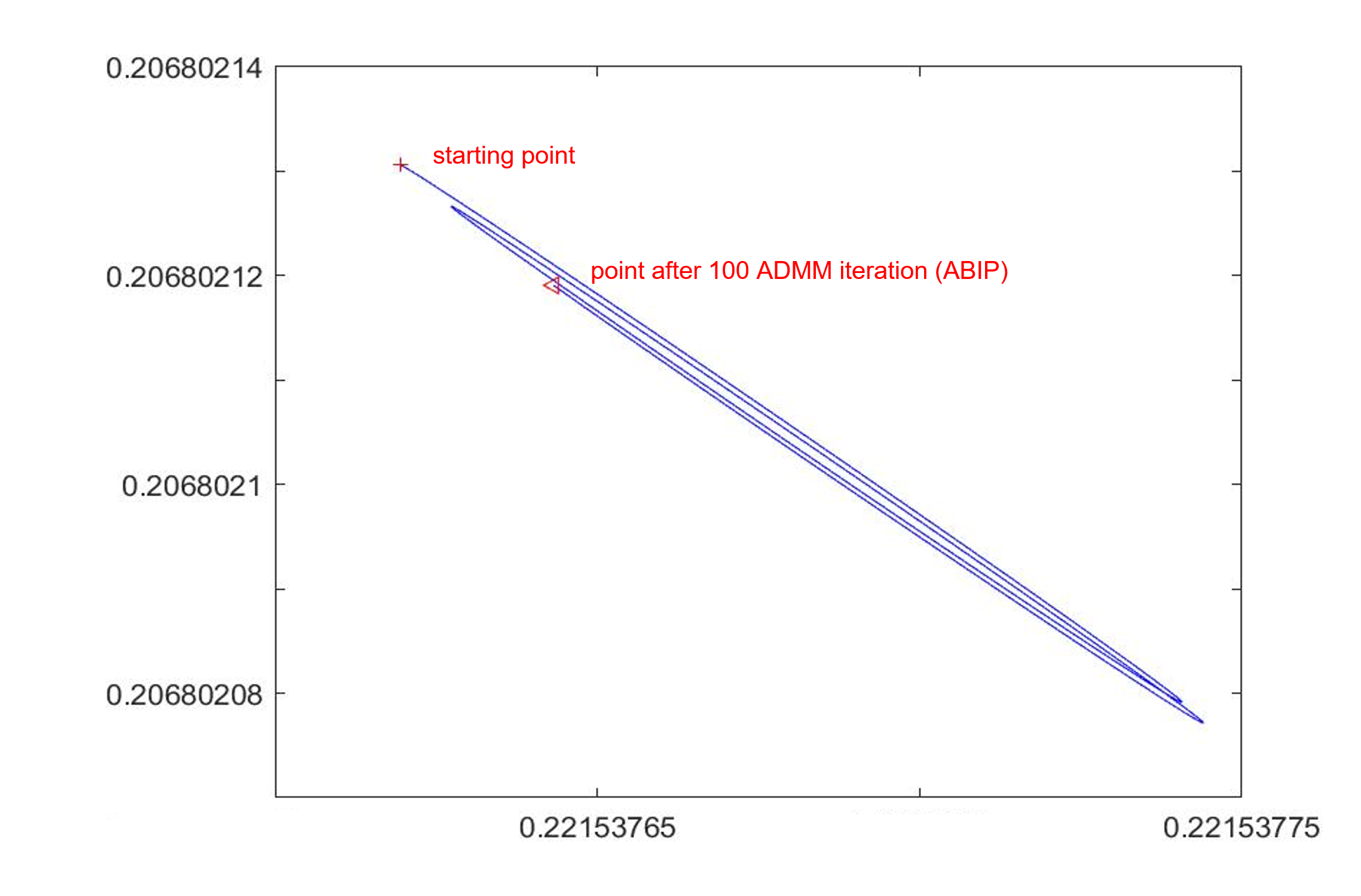
(a) The spiral trajectory of the original ABIP

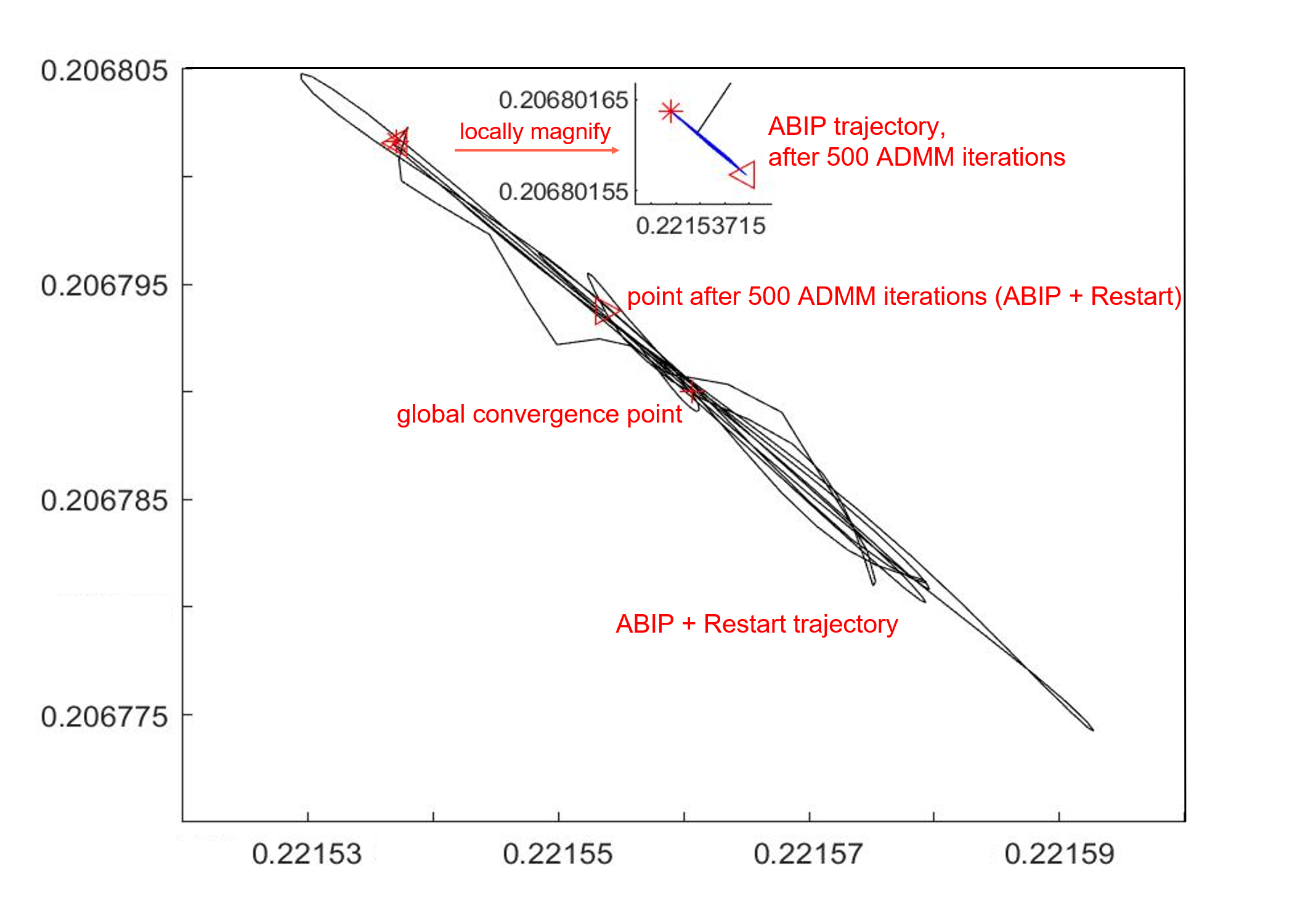
(b) The trajectory of ABIP after restart

Figure 1: Comparison of the trajectories of ABIP after restart and the baseline ABIP

3.3 New inner loop stopping criteria

The original ABIP adopts the criterion (10) to terminate the inner loop. In the enhanced implementation, motivated by the restart scheme, we also use the average of historical iterates

$$\bar{\mathbf{u}}_{i}^{k}=\frac{\sum_{i=1}^{k}\mathbf{u}_{i}^{k}}{k}\quad\text{and}\quad\bar{\mathbf{v}}_{i}^{k}=\frac{\sum_{i=1}^{k}\mathbf{v}_{i}^{k}}{k},$$

and adopt

$$\left\|\mathbf{Q}\bar{\mathbf{u}}_{i}^{k}-\bar{\mathbf{v}}_{i}^{k}\right\|^{2}\leq\mu^{k},$$

as another stopping criterion with the returned solution $(\bar{\mathbf{u}}_{i}^{k},\bar{\mathbf{v}}_{i}^{k})$. When one of the two criteria is satisfied, we terminate the inner loop and take the returned solution as the starting point of the ADMM algorithm to solve the next subproblem in the form of (5).

We also check the global convergence criterion (11) in the inner loop when the penalty parameter $\mu^{k}$ associated with the subproblem (5) satisfies $\mu^{k}<\epsilon$. This is an early-stopping strategy to jump out of the inner loop, which is particularly useful for some ADMM iterates that do not meet the inner loop convergence criterion but already satisfy the global convergence criterion. We remark that the timing of activating this strategy should be chosen carefully. If we check the global convergence criterion too early, the algorithm will waste considerable amount of time computing the primal residual, dual residual, and duality gap for each ADMM iterate that is far from the global optimal point. The numerical experiments demonstrate the effectiveness of this early-stopping strategy.

3.4 Half update

Recall that after eliminating the variables $\mathbf{p},\mathbf{q}$ and $\tilde{\mathbf{v}}$, the ABIP in [20] sequentially updates $\tilde{\mathbf{u}}^{k}_{i+1},\mathbf{u}^{k}_{i+1},\mathbf{v}^{k}_{i+1}$ in each ADMM iteration, where $\mathbf{v}^{k}_{i+1}$ serves the role of dual variable. This motivates us to introduce the half update strategy by updating $\mathbf{v}^{k}$ twice in each of the ADMM iteration for the inner problem (5). In particular, we first update the primal variable $\tilde{\mathbf{u}}_{i+1}^{k}$, followed by the update of dual variable $\mathbf{v}_{i+\frac{1}{2}}^{k}$ with stepsize $\alpha_{1}\in(0,2)$, then we update the primal variable $\mathbf{u}_{i+1}^{k}$, followed by the update of dual variable $\mathbf{v}_{i+1}^{k}$ with stepsize $\alpha_{2}\in(0,2)$. Therefore, the updating rule for $\mathbf{u}^{k}_{i+1}$ is slightly changed as

$$\mathbf{u}_{i+1}^{k}=\underset{\mathbf{u}}{\operatorname{argmin}}\left[\bar{B}\left(\mathbf{u},\mu^{k}\right)+\frac{\beta}{2}\left\|\mathbf{u}-\tilde{\mathbf{u}}_{i+1}^{k}+\mathbf{v}_{i+\frac{1}{2}}^{k}\right\|^{2}\right],$$ (12)

where

$$\bar{B}(\mathbf{u},\mu^{k}):=\beta(n+1)\theta-\mu^{k}\log(\mathbf{x})-\mu^{k}\log\tau.$$

Problem (12) admits closed-form solutions given by

$$\mathbf{y}_{i+1}^{k} =\arg\min_{\mathbf{y}}\frac{\beta}{2}\|\mathbf{y}-\tilde{\mathbf{y}}^{k}_{i+1}+\mathbf{r}^{k}_{i+\frac{1}{2}}\|^{2}=\tilde{\mathbf{y}}^{k}_{i+1}-\mathbf{r}^{k}_{i+\frac{1}{2}}$$ (13)

$$\mathbf{x}_{i+1}^{k} =\arg\min_{\mathbf{x}}\left[-\frac{\mu^{k}}{\beta}\log{(\mathbf{x})}+\frac{1}{2}\left\|\mathbf{x}-\tilde{\mathbf{x}}^{k}_{i+1}+\mathbf{s}^{k}_{i+\frac{1}{2}}\right\|^{2}\right]$$

$$=\frac{1}{2}\left[\left(\tilde{\mathbf{x}}_{i+1}^{k}-\mathbf{s}_{i+\frac{1}{2}}^{k}\right)+\sqrt{\left(\tilde{\mathbf{x}}_{i+1}^{k}-\mathbf{s}_{i+\frac{1}{2}}^{k}\right)\circ\left(\tilde{\mathbf{x}}_{i+1}^{k}-\mathbf{s}_{i+\frac{1}{2}}^{k}\right)+\frac{4\mu^{k}}{\beta}}\right]$$ (14)

$$\tau_{i+1}^{k} =\arg\min_{\tau}\left[-\frac{\mu^{k}}{\beta}\log{\tau}+\frac{1}{2}\left\|\tau-\tilde{\tau}^{k}_{i+1}+\kappa^{k}_{i+\frac{1}{2}}\right\|^{2}\right]$$

$$=\frac{1}{2}\left[\left(\tilde{\tau}_{i+1}^{k}-\kappa_{i+\frac{1}{2}}^{k}\right)+\sqrt{\left(\tilde{\tau}_{i+1}^{k}-\kappa_{i+\frac{1}{2}}^{k}\right)\circ\left(\tilde{\tau}_{i+1}^{k}-\kappa_{i+\frac{1}{2}}^{k}\right)+\frac{4\mu^{k}}{\beta}}\right]$$ (15)

$$\theta^{k}_{i+1} =\tilde{\theta}^{k}_{i+1}-\xi^{k}_{i+\frac{1}{2}}-(n+1)\$$ (16)

However, the termination criterion of the inner problem (5) remains unchanged, i.e.,

$$\left\|\mathbf{Q}\mathbf{u}_{i}^{k}-\mathbf{v}_{i}^{k}\right\|^{2}\leq\mu^{k}.$$

We observe that this strategy can reduce the number of ADMM iterations on some specific datasets. The details of the half update strategy are presented in Algorithm 2.

1 Set $\mu^{0}=\beta>0$, $\alpha,\gamma\in(0,1)$ ;

2 Set $\mathbf{r}^{0}_{0}=\mathbf{y}^{0}_{0}=0$, $(\mathbf{x}^{0}_{0},\tau^{0}_{0},\mathbf{s}^{0}_{0},\kappa^{0}_{0})=(\mathbf{e},1,\mathbf{e},1)>0$, $\theta^{0}_{0}=1$, $\xi^{0}_{0}=-n-1$ with $\mathbf{x}^{0}_{0}\circ\mathbf{s}^{0}_{0}=\frac{\mu^{0}}{\beta}\mathbf{e}$, and $\tau_{0}^{0}\kappa_{0}^{0}=\frac{\mu^{0}}{\beta}$ ;

3 for $k=0,1,2,\cdots$ do

4      for $i=0,1,2,\cdots$ do

5           if the inner termination condition is satisfied then

6                break ;

7                end if

8               Update $\tilde{\mathbf{u}}_{i+1}^{k}$ by (9) ;

9                Update $\mathbf{v}_{i+\frac{1}{2}}^{k}=\alpha\mathbf{u}_{i}^{k}+\textbf{v}_{i}^{k}-\alpha\tilde{\mathbf{u}}_{i+1}^{k}$ ;

10                Update $\mathbf{u}_{i+1}^{k}$ by (13), (14), (15) and (16) ;

11                Update $\mathbf{v}_{i+1}^{k}=\mathbf{v}_{i+\frac{1}{2}}^{k}-\tilde{\mathbf{u}}_{i+1}^{k}+\mathbf{u}_{i+1}^{k}$ ;

12                if the final termination criterion is satisfied then

13                     return ;

14                     end if

15                    

16                     end for

17                    Set $\mu^{k+1}=\gamma\mu^{k}$ ;

18                     Set $\mathbf{r}_{0}^{k+1}=0$, $\xi_{0}^{k+1}=-n-1$ and

$$\left(\mathbf{y}_{0}^{k+1},\mathbf{x}_{0}^{k+1},\mathbf{s}_{0}^{k+1},\tau_{0}^{k+1},\kappa_{0}^{k+1},\theta_{0}^{k+1}\right)=\sqrt{\gamma}\cdot\left(\mathbf{y}_{i+1}^{k},\mathbf{x}_{i+1}^{k},\mathbf{s}_{i+1}^{k},\tau_{i+1}^{k},\kappa_{i+1}^{k},\theta_{i+1}^{k}\right)$$

19                     end for

Algorithm 2 ABIP with half update

3.5 Presolve and preconditioning

Presolve is an important step to transform the input problem into an easier one before starting the optimization algorithm, and it is a essential component in the modern commercial LP solvers. In the enhanced version of ABIP, we include PaPILO [13], an open-source library, for presolve.

After presolve, we obtain a reduced LP problem as follows,

$$\begin{split}\min&\quad\bar{\mathbf{c}}^{T}\bar{\mathbf{x}}\\ \text{s.t.}&\quad\bar{\mathbf{A}}\bar{\mathbf{x}}=\bar{\mathbf{b}}\\ &\quad\bar{\mathbf{x}}\geq 0\\ \end{split}$$

Then, similar to PDLP[1], we perform diagonal preconditioning, which is a popular heuristic to improve the convergence of optimization algorithms. We rescale the constraint matrix $\bar{\mathbf{A}}\in\mathbb{R}^{m\times n}$ to $\tilde{\mathbf{A}}=\mathbf{D}_{1}^{-1}\bar{\mathbf{A}}\mathbf{D}_{2}^{-1}$ with positive diagional matrices $\mathbf{D}_{1}$ and $\mathbf{D}_{2}$. Such preconditioning creates a new LP instance that replace $\bar{\mathbf{A}},\bar{\mathbf{c}},\bar{\mathbf{x}}$ and $\bar{\mathbf{b}}$ with $\tilde{\mathbf{A}}$, $\tilde{\mathbf{c}}=\mathbf{D}_{2}^{-1}\bar{\mathbf{c}}$, $\tilde{\mathbf{x}}=\mathbf{D}_{2}\bar{\mathbf{x}}$ and $\tilde{\mathbf{b}}=\mathbf{D}_{1}^{-1}\bar{b}$, respectively. In particular, we consider two different rescaling tricks, including Pock-Chambolle rescaling and Ruiz rescaling.

• Pock-Chambolle rescaling [26]: It is parameterized by $\alpha>0$, where the diagonal matrices are defined by $(\mathbf{D}_{1})_{jj}=\sqrt{\|\mathbf{A}_{j,\cdot}\|_{2-\alpha}}$ for $j=1,2,\cdots,m$ and $(\mathbf{D}_{2})_{ii}=\sqrt{\|\mathbf{A}_{\cdot,i}\|_{\alpha}}$ for $i=1,2,\cdots,n$. We use $\alpha=1$ in the implementation.

• Ruiz rescaling [28]: In an iteration of Ruiz rescaling, the diagonal matrices are defined by $(\mathbf{D}_{1})_{jj}=\sqrt{\|\mathbf{A}_{j,\cdot}\|_{\infty}}$ for $j=1,2,\cdots,m$ and $(\mathbf{D}_{2})_{ii}=\sqrt{\|\mathbf{A}_{\cdot,i}\|_{\infty}}$ for $i=1,2,\cdots,n$. If the rescaling is applied iteratively, the infinity norm of each row and each column converge to $1$.

In the implementation, we first take a few iterations of Ruiz rescaling and then apply the Pock-Chambolle rescaling.

3.6 Ignoring dual feasibility for null objective problems

We consider the following null objective linear programming

$$\min_{\mathbf{x}} 0$$

s.t. $$\mathbf{A}\mathbf{x}=\mathbf{b}$$

$$\mathbf{x}\geq 0,$$

which is essentially a feasibility problem. Note this class of problem is not artificially constructed, and some real problems have such feature. For instance, the PageRank problem can be formulated as a feasibility problem of a specific linear program [22].

When ABIP is invoked to solve such feasibility problem, the dual is homogeneous and admits a trivial feasible solution $(\mathbf{y},\mathbf{s})=(0,0)$. If ABIP produces a near primal feasible solution $\mathbf{x}$ and approximate dual solution such that $(\mathbf{x}^{\ast},\hat{\mathbf{y}},\hat{\mathbf{s}})$ satisfies

$$\mathbf{A}\mathbf{x}^{\ast} =\mathbf{b},$$

$$\mathbf{A}^{T}\hat{\mathbf{y}}+\hat{\mathbf{s}} =\bm{\delta},$$

$$\mathbf{x}^{\ast},\hat{\mathbf{s}} \geq 0,$$

then we can construct a more accurate interior dual solution by

$$(\mathbf{y}^{\prime},\mathbf{s}^{\prime})=\frac{\varepsilon}{\|\bm{\delta}\|}(\hat{\mathbf{y}},\hat{\mathbf{s}})$$

such that $\|\mathbf{A}^{T}\mathbf{y}^{\prime}+\mathbf{s}^{\prime}\|=\varepsilon$. Although the above observation cannot be used to identify the support of the optimal $\mathbf{s}^{\ast}$, it implies that we don’t need to check dual infeasibility when the algorithm iterates to obtain a near-feasible primal-dual pair in ABIP.

3.7 Strategy integration

As mentioned above, we propose various computational strategies to improve empirical performance of ABIP. Each strategy has some parameters to choose, and thus one critical issue is how to determine which combination of parameters in the strategies that can lead to good empirical performance. To resolve this issue, a decision tree is embedded in ABIP to help identify the rules for choosing a proper combination of strategies. More specifically, for each LP instance, we collect the sparsity and dimension related statistics of the problem as features, and test the run time of ABIP under different combinations of strategies. Then the combination costing least time is recorded as the label.

To avoid overfitting, we restrict the number of combinations of strategies to be $3$ and run the test over a large collection of datasets including MIPLIB 2017 [14] and Netlib LP [19]. In addition, after the decision tree is obtained from the training procedure, we prune the tree till the rules left is general enough to be coded by the solver.

Figure 2: Decision tree for ABIP

The computational experiments suggest that the decision tree is often able to capture desirable features for LPs and the derived decision rules prove effective in practice.

4 ABIP for conic programming

Our next goal is to extend ABIP to solving the more general linear program for which the constraint set $\mathcal{K}$ is a general convex cone.

Motivating problems

A strong motivation for our work is to solve the following quadratic problem

$$\min_{\mathbf{z}} \quad\frac{1}{2}\mathbf{z}^{T}\mathbf{P}\mathbf{z}+\mathbf{q}^{T}\mathbf{z}$$ (17)

s.t. $$\quad\bar{\mathbf{A}}\mathbf{z}=\bar{\mathbf{b}}$$

$$\quad\mathbf{z}\geq 0$$

where $\bar{\mathbf{A}}\in\mathbb{R}^{m\times n}$ and $\mathbf{P}\in\mathbb{R}^{n\times n}$ is a positive semi-definite matrix. Convex quadratic programming has extensive applications in machine learning and data science, such as SVM [7], Lasso [33] and portfolio optimization. However, due to the additional quadratic term in the objective, problem (17) can not be directly solved by ABIP for linear programming.

Problems (17) can be formulated as a conic programming in the following manner. Consider $\mathcal{K}$ to be any Cartesian product of primitive cones, i.e.

$$\mathcal{K} =\text{SOCs}\times\text{RSOCs}\times\mathbb{R}^{f}\times\{0\}^{z}\times\mathbb{R}_{+}^{l},$$

$$\mathcal{K}^{*} =\text{SOCs}\times\text{RSOCs}\times\{0\}^{f}\times\mathbb{R}^{z}\times\mathbb{R}_{+}^{l},$$

Here, SOCs and RSOCs represent Cartesian products of multiple regular second-order cones and rotated second-order cones, respectively; constants $f$, $z$, $l$ are dimensions of free variables, zero variables and non-negative variables, respectively. Let $\mathbf{P}=\bm{\Lambda}^{T}\bm{\Lambda}$ be the factorization where $\bm{\Lambda}\in\mathbb{R}^{r\times n}$, problem (17) can be expressed as the following problem

$$\min \quad\frac{1}{2}\bar{\mathbf{x}}^{T}\bar{\mathbf{x}}+\mathbf{q}^{T}\bar{\mathbf{z}}$$

s.t. $$\quad\bar{\mathbf{A}}\bar{\mathbf{z}}=\bar{\mathbf{b}}$$

$$\quad\bar{\mathbf{x}}=\Lambda\bar{\mathbf{z}}$$

$$\quad\bar{\mathbf{z}}\geq 0$$

which can be further translated to the conic form:

$$\begin{aligned} \min&\quad\nu+\mathbf{q}^{T}\bar{\mathbf{z}}\\ \text{s.t.}&\quad\eta=1\\ &\quad\bar{\mathbf{A}}\bar{\mathbf{z}}=\bar{\mathbf{b}}\\ &\quad\bar{\mathbf{x}}=\bm{\Lambda}\bar{\mathbf{z}}\\ &\quad\eta\nu\geq\frac{1}{2}\bar{\mathbf{x}}^{T}\bar{\mathbf{x}}\\ &\quad\bar{\mathbf{z}}\geq 0\end{aligned}\ \Leftrightarrow\ \begin{aligned} \min&\quad\begin{bmatrix}0\\ 1\\ \mathbf{0}_{r\times 1}\\ \mathbf{q}\end{bmatrix}^{T}\begin{bmatrix}\eta\\ \nu\\ \bar{\mathbf{x}}\\ \bar{\mathbf{z}}\end{bmatrix}\\ \text{s.t.}&\quad\begin{bmatrix}1\\ &\mathbf{0}_{r\times 1}&\mathbf{I}_{r}&-\bm{\Lambda}\\ &&&\bar{\mathbf{A}}\end{bmatrix}\begin{bmatrix}\eta\\ \nu\\ \bar{\mathbf{x}}\\ \bar{\mathbf{z}}\end{bmatrix}=\begin{bmatrix}1\\ \mathbf{0}_{r\times 1}\\ \bar{\mathbf{b}}\end{bmatrix}\\ &\quad(\eta,\nu,\bar{\mathbf{x}})\in\text{RSOC}_{2+r},\bar{\mathbf{z}}\in\mathbb{R}_{+}^{n}\end{aligned}$$

where $\mathbf{I}_{r}$ is $r$-dimensional identity matrix.

It should be noted that while we mainly focus on the applications of quadratic optimization, the conic formulation (1), as well as our subsequent algorithm development and convergence analysis, are developed for the general convex conic programs such as SDP. Nevertheless, detailed performance study beyond the SOCP setting will be left to our future work.

Homogeneous self-dual embedding for conic programming

Before extending ABIP to conic problem, we briefly describe the HSD embedding technique for convex conic optimization [21, 44]. Given an initial solution $\mathbf{x}^{0}\in\text{int}\>\mathcal{K},\mathbf{s}^{0}\in\text{int}\>\mathcal{K}^{*}$ and $\mathbf{y}^{0}\in\mathbb{R}^{m}$, we can derive the following homogeneous self-dual embedding:

$$\min \quad\left((\mathbf{x}^{0})^{T}\mathbf{s}^{0}+1\right)\theta$$ (18)

s.t. $$\quad\mathbf{A}\mathbf{x}-\mathbf{b}\tau+\mathbf{r}_{p}\theta=\mathbf{0}$$

$$\quad-\mathbf{A}^{T}\mathbf{y}+\mathbf{c}\tau+\mathbf{r}_{d}\theta=\mathbf{s}$$

$$\quad\mathbf{b}^{T}\mathbf{y}-\mathbf{c}^{T}\mathbf{x}+r_{g}\theta=\kappa$$

$$\quad-\mathbf{r}_{p}^{T}\mathbf{y}-\mathbf{r}_{d}^{T}\mathbf{x}-r_{g}\tau=-(\mathbf{x}^{0})^{T}\mathbf{s}^{0}-1$$

$$\quad\mathbf{x}\in\mathcal{K},\mathbf{s}\in\mathcal{K}^{*},\tau,\kappa\geq 0$$

where $\mathbf{r}_{p}=\mathbf{b}-\mathbf{A}\mathbf{x}^{0}$, $\mathbf{r}_{d}=\mathbf{s}^{0}-\mathbf{c}+\mathbf{A}^{T}\mathbf{y}^{0}$, $r_{g}=1+\mathbf{c}^{T}\mathbf{x}^{0}-\mathbf{b}^{T}\mathbf{y}^{0}$. It is easy to check that the constraint matrix of (18) is skew-symmetric and hence the above system is self-dual. The conic HSD (18) enjoys several attractive properties [44, 21], which we list below.

Proposition 1.

The system (18) is strictly feasible. Specifically, there is a strictly feasible solution $(\mathbf{y},\mathbf{x},\tau,\theta,\mathbf{s},\kappa)$ such that

$$\mathbf{y}=\mathbf{y}^{0},\mathbf{x}=\mathbf{x}^{0},\tau=1,\theta=1,\mathbf{s}=\mathbf{s}^{0},\kappa=1.$$

Proposition 2.

The problem (18) has a maximally complementary optimal solution, denoted by $\left(\mathbf{y}^{*},\mathbf{x}^{*},\tau^{*},\theta^{*},\mathbf{s}^{*},\kappa^{*}\right)$, such that $\theta^{*}=0$ and $(\mathbf{x}^{*})^{T}\mathbf{s}^{*}+\tau^{*}\kappa^{*}=0$. Moreover, if $\tau^{*}>0$, then $\frac{\mathbf{x}^{*}}{\tau^{*}}$ is an optimal solution for (P), and $(\frac{\mathbf{y}^{*}}{\tau^{*}},\frac{\mathbf{s}^{*}}{\tau^{*}})$ is an optimal solution for (D). If $\kappa^{*}>0$ then either $\mathbf{c}^{T}\mathbf{x}^{*}<0$ or $\mathbf{b}^{T}\mathbf{y}^{*}>0$; in the former case (D) is infeasible, and in the latter case (P) is infeasible.

4.1 Algorithmic development

Our algorithm follows from the development of ABIP for LP. For the sake of completeness, we give a full description of the conic extension. Problem (18) can be rewritten as

$$\min \quad\beta((\mathbf{x}^{0})^{T}\mathbf{s}^{0}+1)\theta+\mathds{1}(\mathbf{r}=0)+\mathds{1}(\xi=-(\mathbf{x}^{0})^{T}\mathbf{s}^{0}-1)$$ (19)

s.t. $$\quad\mathbf{Q}\mathbf{u}=\mathbf{v}$$

$$\quad(\mathbf{x},\mathbf{s},\tau,\kappa)\in\mathcal{K}\times\mathcal{K}^{*}\times\mathbb{R}_{+}\times\mathbb{R}_{+},\ \mathbf{y},\theta\ \text{free}.$$

where $\mathbf{Q},\mathbf{u},\mathbf{v}$ are defined in (3). Next, we follow the interior point method by replacing the conic constraints with barrier penalties in the objective. Let $F(\mathbf{x})$ and $G(\mathbf{s})$ be the logarithmic barrier functions associated with $\mathcal{K}$ and $\mathcal{K}^{*}$, respectively, and define the objective

$$B(\mathbf{u},\mathbf{v},\mu) =\beta((\mathbf{x}^{0})^{T}\mathbf{s}^{0}+1)\theta+\mathds{1}(\mathbf{r}=0)+\mathds{1}(\xi=-(\mathbf{x}^{0})^{T}\mathbf{s}^{0}-1)$$ (20)

$$\quad+\mu F(\mathbf{x})+\mu G(\mathbf{s})-\mu\log\tau-\mu\log\kappa.$$

ABIP successively solves a series of penalized problems

$$\min B(\mathbf{u},\mathbf{v},\mu^{k})$$ (21)

s.t. $$\mathbf{Q}\mathbf{u}=\mathbf{v}$$

for a sequence of diminishing penalty weights $\mu^{k}$: $\lim_{k\rightarrow\infty}\mu^{k}=0$. By using variable splitting, (21) is equivalent to the following constrained problem

$$\min \mathds{1}(\mathbf{Q}\tilde{\mathbf{u}}=\tilde{\mathbf{v}})+B(\mathbf{u},\mathbf{v},\mu^{k})$$ (22)

s.t. $$(\tilde{\mathbf{u}},\tilde{\mathbf{v}})=(\mathbf{u},\mathbf{v})$$

Subsequently, ADMM is applied to obtain an approximate solution of the resulting constrained problem (22).

Let us denote augmented Lagrangian function by

$$\mathcal{L}_{\beta}(\tilde{\mathbf{u}},\tilde{\mathbf{v}},\mathbf{u},\mathbf{v},\mu^{k},\mathbf{p},\mathbf{q})=\mathds{1}(\mathbf{Q}\tilde{\mathbf{u}}=\tilde{\mathbf{v}})+B(\mathbf{u},\mathbf{v},\mu^{k})-\langle\beta(\mathbf{p},\mathbf{q}),(\tilde{\mathbf{u}},\tilde{\mathbf{v}})-(\mathbf{u},\mathbf{v})\rangle+\frac{\beta}{2}\|(\tilde{\mathbf{u}},\tilde{\mathbf{v}})-(\mathbf{u},\mathbf{v})\|^{2},$$

where $\beta>0$ is the same parameter as the one in (19), and $p$, $q$ are the Lagrangian multipliers associated with the linear constraints. Recall that the $i$-th iteration of ADMM for solving (22) is (6), (7) and (8). For practical implementation, Lin et al. [20] shows that the ADMM iteration can be substantially simplified, resulting in much more efficient implementation.

We show that this attractive feature of ADMM still holds for the more general conic programming.

Theorem 1.

For the $k$-th outer iteration of ABIP, we initialize $\mathbf{p}^{k}_{0}=\mathbf{v}^{k}_{0}$ and $\mathbf{q}^{k}_{0}=\mathbf{u}^{k}_{0}$. It then holds, for all iterations $i\geq 0$, that $\mathbf{p}^{k}_{i}=\mathbf{v}^{k}_{i}$ and $\mathbf{q}^{k}_{i}=\mathbf{u}^{k}_{i}$.

Proof.

Proof. We shall prove the result by induction. (i) At iteration $j=0$, the result holds true from our definition. (ii) Assuming it holds true for iteration $j=i$, we will prove that the result still holds true for iteration $j=i+1$ in two steps:

Step 1: We claim that

$$\mathbf{u}^{k}_{i}+\mathbf{v}^{k}_{i}=\tilde{\mathbf{u}}^{k}_{i+1}+\tilde{\mathbf{v}}^{k}_{i+1}.$$ (23)

Indeed, (6) can be rewritten as

$$(\tilde{\mathbf{u}}^{k}_{i+1},\tilde{\mathbf{v}}^{k}_{i+1})=\Pi_{\mathcal{P}}(\mathbf{u}^{k}_{i}+\mathbf{v}^{k}_{i},\mathbf{u}^{k}_{i}+\mathbf{v}^{k}_{i}),$$ (24)

where $\mathcal{P}=\{(\mathbf{u},\mathbf{v}):\mathbf{Q}\mathbf{u}=\mathbf{v}\}$. Moreover, since $\mathbf{Q}$ is skew-symmetric, the orthogonal complement of $\mathcal{P}$ is $\mathcal{P}^{\perp}=\{(\mathbf{v},\mathbf{u}):\mathbf{Q}\mathbf{u}=\mathbf{v}\}$. Therefore, we conclude that

$$(\mathbf{u},\mathbf{v})=\Pi_{\mathcal{P}}(\mathbf{z},\mathbf{z})\quad\text{if and only if}\quad(\mathbf{v},\mathbf{u})=\Pi_{\mathcal{P}^{\perp}}(\mathbf{z},\mathbf{z}),$$

because the two projections are identical for reversed output arguments. This implies that

$$(\tilde{\mathbf{v}}^{k}_{i+1},\tilde{\mathbf{u}}^{k}_{i+1})=\Pi_{\mathcal{P}^{\perp}}(\mathbf{u}^{k}_{i}+\mathbf{v}^{k}_{i},\mathbf{u}^{k}_{i}+\mathbf{v}^{k}_{i}).$$ (25)

Then we combine (24) and (25) to get the desired result.

Step 2: Given $\mathbf{p}^{k}_{i}=\mathbf{v}^{k}_{i}$, $\mathbf{q}^{k}_{i}=\mathbf{u}^{k}_{i}$ and $\xi^{k}_{i}=-\mathbf{x}_{0}^{T}\mathbf{s}_{0}-1$, our goal is to show that

$$\mathbf{p}^{k}_{i+1}=\mathbf{v}^{k}_{i+1},\quad\mathbf{q}^{k}_{i+1}=\mathbf{u}^{k}_{i+1}.$$

Note that (23) can be rewritten as

$$\tilde{\mathbf{u}}^{k}_{i+1}-\mathbf{v}^{k}_{i}=-(\tilde{\mathbf{v}}^{k}_{i+1}-\mathbf{u}^{k}_{i}).$$

We denote $\sigma=\tilde{\mathbf{u}}^{k}_{i+1}-\mathbf{v}^{k}_{i}$. It is easy to verify that functions in (20) form pairs of function $h(t)$ and $w(t)$ satisfying $w(t)=h^{*}(-t)$, where $h^{*}$ denotes the conjugate function of $h$. From Moreau’s decomposition (see Section 2.5 in [6] for more details), for such pairs of functions $(h(t),w(t))$ in $B$, we have

$$\mathbf{u}^{k}_{i+1}-\mathbf{v}^{k}_{i+1}=\text{prox}_{h}(\sigma)-\text{prox}_{w}(-\sigma)=\sigma.$$

Then from (8) we have

$$\mathbf{p}^{k}_{i+1} =\mathbf{v}^{k}_{i}+\mathbf{u}^{k}_{i+1}-\tilde{\mathbf{u}}^{k}_{i+1}=\mathbf{u}^{k}_{i+1}-\sigma=\mathbf{v}^{k}_{i+1},$$

$$\mathbf{q}^{k}_{i+1} =\mathbf{u}^{k}_{i}+\mathbf{v}^{k}_{i+1}-\tilde{\mathbf{v}}^{k}_{i+1}=\mathbf{v}^{k}_{i+1}+\sigma=\mathbf{u}^{k}_{i+1}.$$

This completes the proof.∎

Specifically, Theorem 1 implies that by carefully choosing the initial point (i.e. setting $\mathbf{u}_{0}^{k}=\mathbf{v}_{0}^{k}$), we can eliminate the dual variables $\mathbf{p}^{k},\mathbf{q}^{k}$ safely for conic programs. Moreover, following a similar argument of [20], one can use the skew-symmetry of $\mathbf{Q}$ to obtain a simple update for $\tilde{\mathbf{u}}^{k+1}$ and use (8) to eliminate $\tilde{\mathbf{v}}_{i+1}^{k}$. In a nutshell, the ADMM inner loop (6), (7) and (8) in the $k$-th ABIP iteration can be simplified as

$$\tilde{\mathbf{u}}^{k}_{i+1} =(\mathbf{I}+\mathbf{Q})^{-1}(\mathbf{u}^{k}_{i}+\mathbf{v}^{k}_{i}),$$ (26)

$$\mathbf{u}^{k}_{i+1} =\textrm{prox}_{\bar{B}_{\mu}/\beta}(\tilde{\mathbf{u}}^{k}_{i+1}-\mathbf{v}^{k}_{i}),$$ (27)

$$\mathbf{v}^{k}_{i+1} =\mathbf{v}^{k}_{i}-\tilde{\mathbf{u}}^{k}_{i+1}+\mathbf{u}^{k}_{i+1}.$$ (28)

Here, $\bar{B}_{\mu}(\mathbf{u})$ is the penalty function $B(\mathbf{u},\mathbf{v},\mu)$ restricted to the $\mathbf{u}$ part: $\bar{B}_{\mu}(\mathbf{u})=\beta((\mathbf{x}^{0})^{T}\mathbf{s}^{0}+1)\theta+\mathds{1}(\mathbf{r}=0)+\mathds{1}(\xi=-(\mathbf{x}^{0})^{T}\mathbf{s}^{0}-1)+\mu F(\mathbf{x})-\mu\log\tau$, and we denote the proximal operator by $\operatornamewithlimits{prox}_{f}(\mathbf{x})=\operatorname*{argmin}_{\bar{\mathbf{u}}}\{f(\bar{\mathbf{u}})+\frac{1}{2}\|\bar{\mathbf{u}}-\mathbf{u}\|^{2}\}$.

In each inner loop, we use the following criteria as the termination criteria.

$$||\mathbf{Q}\mathbf{u}_{N_{k}}^{k}-\mathbf{v}_{N_{k}}^{k}||^{2}\leq\mu^{k}.$$ (29)

4.2 Convergence analysis

Our next goal is to develop the iteration complexity of the ABIP method, for which we generalize the analysis of [20] to the conic setting. The analysis consists of three steps. First, we show that points generated by the ADMM iterations are uniformly bounded above. Second, based on the uniform boundedness, we show that in the inner loop, ABIP exhibits a linear convergence to the optimal subproblem solution. Third, in view of the path-following scheme, we derive the total iteration complexity of ABIP.

Let $(\mathbf{u}_{k}^{*},\mathbf{v}_{k}^{*})$ be the optimal solution of problem (22), it can be shown that $(\mathbf{u}_{i}^{k},\mathbf{v}_{i}^{k})$ converges to $(\mathbf{u}_{k}^{*},\mathbf{v}_{k}^{*})$. We state this result in the following proposition.We strictly follow the proof Lemma 3.4 [20] and hence skip it for brevity.

Proposition 3.

For a fixed $k\in\mathbb{N}_{+}$, the sequence $\{||\mathbf{u}_{i}^{k}-\mathbf{u}_{k}^{*}||^{2}+||\mathbf{v}_{i}^{k}-\mathbf{v}_{k}^{*}||^{2}\}$ is monotonically decreasing and converges to 0.

Then we prove the uniformly-boundedness of the points in all iterations. Since for any fixed $k$, the sequence $\{||\mathbf{u}_{i}^{k}-\mathbf{u}_{k}^{*}||^{2}+||\mathbf{v}_{i}^{k}-\mathbf{v}_{k}^{*}||^{2}\}$ is monotonically decreasing, we only need to prove the boundedness of $\{||\mathbf{u}_{0}^{k}-\mathbf{u}_{k}^{*}||^{2}+||\mathbf{v}_{0}^{k}-\mathbf{v}_{k}^{*}||^{2}\}$.

Proposition 4.

The sequence $\{||\mathbf{u}_{i}^{k}-\mathbf{u}_{k}^{*}||^{2}+||\mathbf{v}_{i}^{k}-\mathbf{v}_{k}^{*}||^{2}\}$ is uniformly bounded.

Proof.

Proof. We first assume that the central path is in the ball of radius $\sqrt{C_{1}}$ centered at the origin, Namely, for $k=1,2,\ldots,$, the following result

$$||\mathbf{u}_{k}^{*}||^{2}+||\mathbf{v}_{k}^{*}||^{2}\leq C_{1}$$

holds. Let $(\mathbf{u}^{*},\mathbf{v}^{*})$ be the limit point of $(\mathbf{u}_{k}^{*},\mathbf{v}_{k}^{*})$, then $(\mathbf{u}^{*},\mathbf{v}^{*})$ also satisfies $||\mathbf{u}^{*}||^{2}+||\mathbf{v}^{*}||^{2}\leq C_{1}$. We claim that when $k\to\infty$, $||\mathbf{u}_{N_{k}}^{k}-\mathbf{u}^{*}||^{2}+||\mathbf{v}_{N_{k}}^{k}-\mathbf{v}^{*}||\to 0$. Otherwise there exists $\delta>0$ and a subsequence $\{k_{t}\}_{t\in\mathbb{N}^{+}}$ such that $||\mathbf{u}_{N_{k_{t}}}^{k_{t}}-\mathbf{u}^{*}||^{2}+||\mathbf{v}_{N_{k_{t}}}^{k_{t}}-\mathbf{v}^{*}||>\delta$ for all $t\in\mathbb{N}^{+}$, and there exists an integer $T$ such that $||\mathbf{u}_{N_{k_{t}}}^{k_{t}}-\mathbf{u}_{k_{t}}^{*}||^{2}+||\mathbf{v}_{N_{k_{t}}}^{k_{t}}-\mathbf{v}_{k_{t}}^{*}||>\delta/2$ for all $t>T$, which contradicts with (29). Therefore $||\mathbf{u}_{N_{k}}^{k}-\mathbf{u}^{*}||^{2}+||\mathbf{v}_{N_{k}}^{k}-\mathbf{v}^{*}||\to 0$ when $k\to\infty$, which also implies that there exists $C_{2}$ such that

$$||\mathbf{u}_{N_{k}}^{k}||^{2}+||\mathbf{v}_{N_{k}}^{k}||^{2}\leq C_{2}.$$

Since $\mathbf{u}_{N_{k}}^{k}=\mathbf{u}_{0}^{k+1}$ and $\mathbf{v}_{N_{k}}^{k}=\mathbf{v}_{0}^{k+1}$, we have proven the boundedness of the sequence $\{\mathbf{v}_{0}^{k}\}$, and by the results of Proposition 3 we have that $\{(\mathbf{u}_{i}^{k},\mathbf{v}_{i}^{k})\}$ is uniformly bounded. ∎

In practice, the algorithm converges well enough if we choose the termination criteria in the inner loop to be $||\mathbf{Q}\mathbf{u}_{i}^{k}-\mathbf{v}_{i}^{k}||\leqslant(\mu^{k})^{\alpha}(1+||(\mathbf{u}_{i}^{k},\mathbf{v}_{i}^{k})||)$, where $\alpha$ is a real number on $[0.25,2]$ chosen according to specific problems.

Finally, we give an upper bound of steps at each inner loop and analyze the iteration complexity of the whole algorithm.

Proposition 5.

The number of iteration in each inner loop $N_{k}$ satisfies

$$N_{k}\leq\log\left(\dfrac{4C_{1}(1+||\mathbf{Q}||^{2})}{\mu^{k}}\right)\left[\log\left(1+\min\left\{\dfrac{1}{C_{3}},\dfrac{\mu^{k}}{2C_{D}C_{3}\beta}\right\}\right)\right]^{-1},$$

where

$$C_{3}=\left[1+\dfrac{12\lambda_{\max}(\mathbf{A}^{T}\mathbf{A})}{\lambda^{2}_{\min}(\mathbf{A}\mathbf{A}^{T})}\max\{1,||\mathbf{c}||^{2},||\mathbf{r}_{d}||^{2}\}\right]\cdot\left[1+\dfrac{6}{||\mathbf{r}_{p}||^{2}}\max\{||\mathbf{b}||^{2},||\mathbf{A}||^{2}\}\right].$$

The next theorem develops the iteration complexity of ABIP for solving conic linear optimization.

Theorem 2.

ABIP requires a total number of $T_{1}=\mathcal{O}\left(\log(\frac{1}{\epsilon})\right)$ outer loops and $T_{2}=\mathcal{O}\big{(}\frac{\kappa_{A}^{2}||\mathbf{Q}||^{2}}{\epsilon}\log\big{(}\frac{1}{\epsilon}\big{)}\big{)}$ ADMM iterations to reach $\mu^{k}<\epsilon$.

Proof.

Proof. Note that ABIP is a double-loop procedure. The outer loop is terminated when $\mu^{k}<\epsilon$, where $\epsilon>0$ is a pre-specified tolerance level. It is easy to see that the number of outer loops is

$$T_{\texttt{IPM}}=\Big{\lceil}\dfrac{\log(\mu^{0}/\epsilon)}{\log(1/\gamma)}\Big{\rceil}.$$

For the total number of ADMM iterations, we have the following bound:

$$T_{\texttt{ADMM}} =\sum_{k=1}^{T_{\texttt{IPM}}}N_{k}\leq\sum_{k=1}^{T_{\texttt{IPM}}}\log\left(\dfrac{4C_{1}(1+||\mathbf{Q}||^{2})}{\mu^{k}}\right)\left[\log\left(1+\min\left\{\dfrac{1}{C_{3}},\dfrac{\mu^{k}}{2C_{D}C_{3}\beta}\right\}\right)\right]^{-1}$$

$$=\sum_{k=1}^{T_{\texttt{IPM}}}\log\left(\dfrac{4C_{1}(1+||\mathbf{Q}||^{2})}{\mu^{0}\gamma^{k}}\right)\left[\log\left(1+\min\left\{\dfrac{1}{C_{3}},\dfrac{\mu^{k}}{2C_{D}C_{3}\beta}\right\}\right)\right]^{-1}$$

$$=O\left(\dfrac{\kappa_{A}^{2}||\mathbf{Q}||^{2}}{\epsilon}\log\left(\dfrac{1}{\epsilon}\right)\right).$$

∎

4.3 Solving the proximal subproblem

For linear programming, we have shown that the proximal mapping to update primal variable $\mathbf{x}$ exhibits a closed-form solution (i.e. eq.(14)). This section aims to show that the proximal problem, for the barrier functions associated with other cones, can be efficiently computed. In particular, we will develop routines for second-order cones and semidefinite cones.

4.3.1 Second-order cone

We shall solve the following proximal subproblem

$$\mathbf{x}^{*}=\operatorname*{argmin}_{\mathbf{x}}\ \lambda F(\mathbf{x})+\frac{1}{2}\|\mathbf{x}-\bm{\zeta}\|_{2}^{2}$$ (30)

where $\lambda>0$ and $\bm{\zeta}$ is a column vector. Here we consider two types of second-order cone: regular second-order cone (SOC) and rotated second-order cone (RSOC), which are listed below

$$\text{SOC}_{1+n_{\mathbf{x}}} =\{(t,\mathbf{x})\in\mathbb{R}\times\mathbb{R}^{n_{\mathbf{x}}}:t\geq\|\mathbf{x}\|_{2}\},$$

$$\text{RSOC}_{2+n_{\mathbf{x}}} =\left\{(\eta,\nu,\mathbf{x})\in\mathbb{R}_{+}\times\mathbb{R}_{+}\times\mathbb{R}^{n_{\mathbf{x}}}:\eta\nu\geq\frac{1}{2}\|\mathbf{x}\|_{2}^{2}\right\}.$$

We show that the associated proximal subproblems in both cases have closed form solutions and thus can be solved efficiently. We leave the technical details to Appendix B.

In the case of SOC and for $\mathbf{x}=(t,\bar{\mathbf{x}})\in\text{SOC}$, the barrier function is $F(\mathbf{x})=-\log\left(t^{2}-\bar{\mathbf{x}}^{T}\bar{\mathbf{x}}\right)$. For convenience, we let $\bm{\zeta}=(\zeta_{t},\bm{\zeta}_{\bar{\mathbf{x}}})^{T}$ and discuss two situations. 1) If $\zeta_{t}=0$, we have

$$t^{*}=\sqrt{2\lambda+\frac{1}{4}\bm{\zeta}_{\bar{\mathbf{x}}}^{T}\bm{\zeta}_{\bar{\mathbf{x}}}},\quad\bar{\mathbf{x}}^{*}=\frac{1}{2}\bm{\zeta}_{\bar{\mathbf{x}}}.$$

2) If $\zeta_{t}\neq 0$, we define $\rho_{1}$ and $\rho_{2}$ as

$$\rho_{1}=\frac{\gamma-\sqrt{\gamma^{2}-16}}{2}<2,\quad\text{and}\quad\rho_{2}=\frac{\gamma+\sqrt{\gamma^{2}-16}}{2}>2,$$

respectively, where $\gamma=\frac{\frac{\zeta_{t}^{2}-\bm{\zeta}_{\bar{\mathbf{x}}}^{T}\bm{\zeta}_{\bar{\mathbf{x}}}}{\lambda}+\sqrt{\left(\frac{\zeta_{t}^{2}-\bm{\zeta}_{\bar{\mathbf{x}}}^{T}\bm{\zeta}_{\bar{\mathbf{x}}}}{\lambda}\right)^{2}+4\left(\frac{4\zeta_{t}^{2}+4\bm{\zeta}_{\bar{\mathbf{x}}}^{T}\bm{\zeta}_{\bar{\mathbf{x}}}}{\lambda}+16\right)}}{2}.$ Then, we obtain the solution

$$t^{*}=\frac{\rho}{\rho-2}\zeta_{t},\quad\bar{\mathbf{x}}^{*}=\frac{\rho}{\rho+2}\bm{\zeta}_{\bar{\mathbf{x}}},$$

where we set $\rho=\rho_{1}$ if $\zeta_{t}<0$ or set $\rho=\rho_{2}$ if $\zeta_{t}>0$.

In the case of RSOC, let $\mathbf{x}=(\eta,\nu,\bar{\mathbf{x}})\in\text{RSOC}$ and denote the barrier function by $F(\mathbf{x})=-\log\left(\eta\nu-\frac{1}{2}\bar{\mathbf{x}}^{T}\bar{\mathbf{x}}\right)$. For convenience, we let $\bm{\zeta}=(\zeta_{\eta},\zeta_{\nu},\bm{\zeta}_{\bar{\mathbf{x}}})^{T}$ and discuss two situations. 1) If $\zeta_{\eta}+\zeta_{\nu}=0$, we have

$$\eta^{*}=\frac{\zeta_{\eta}+\sqrt{\zeta_{\eta}^{2}+4\left(\lambda+\frac{1}{8}\bm{\zeta}_{\bar{\mathbf{x}}}^{T}\bm{\zeta}_{\bar{\mathbf{x}}}\right)}}{2},\quad\nu^{*}=\frac{-\zeta_{\eta}+\sqrt{\zeta_{\eta}^{2}+4\left(\lambda+\frac{1}{8}\bm{\zeta}_{\bar{\mathbf{x}}}^{T}\bm{\zeta}_{\bar{\mathbf{x}}}\right)}}{2},\quad\bar{\mathbf{x}}^{*}=\frac{1}{2}\bm{\zeta}_{\bar{\mathbf{x}}}.$$

2) If $\zeta_{\eta}+\zeta_{\nu}\neq 0$, we define $\rho_{1}$ and $\rho_{2}$ as

$$\rho_{1}=\frac{\gamma-\sqrt{\gamma^{2}-4}}{2}<1,\quad\rho_{2}=\frac{\gamma+\sqrt{\gamma^{2}-4}}{2}>1,$$

where

$$\gamma=\frac{\frac{2\zeta_{\eta}\zeta_{\nu}-\bm{\zeta}_{\bar{\mathbf{x}}}^{T}\bm{\zeta}_{\bar{\mathbf{x}}}}{2\lambda}+\sqrt{\left(\frac{2\zeta_{\eta}\zeta_{\nu}-\bm{\zeta}_{\bar{\mathbf{x}}}^{T}\bm{\zeta}_{\bar{\mathbf{x}}}}{2\lambda}\right)^{2}+4\left(\frac{\zeta_{\eta}^{2}+\zeta_{\nu}^{2}+\bm{\zeta}_{\bar{\mathbf{x}}}^{T}\bm{\zeta}_{\bar{\mathbf{x}}}}{\lambda}+4\right)}}{2}.$$

Then, we have

$$\eta^{*}=\frac{\rho^{2}\zeta_{\eta}+\rho\zeta_{\nu}}{(\rho+1)(\rho-1)},\quad\nu^{*}=\frac{\rho\zeta_{\eta}+\rho^{2}\zeta_{\nu}}{(\rho+1)(\rho-1)}\quad\text{and}\quad\bar{\mathbf{x}}^{*}=\frac{\rho\bm{\zeta}_{\bar{\mathbf{x}}}}{\rho+1},$$

where we set $\rho=\rho_{1}$ if $\zeta_{\eta}+\zeta_{\nu}<0$ or $\rho=\rho_{2}$ if $\zeta_{\eta}+\zeta_{\nu}>0$.

4.3.2 Semidefinite cone

Let us consider the semidefinite cone (SDC) $\mathcal{K}=\{\mathbf{X}:\mathbf{X}\in\mathbb{R}^{n\times n},\mathbf{X}\succeq 0\}$. The associated barrier function is $F(\mathbf{X})=-\log\det(\mathbf{X})$. We shall solve the following proximal subproblem

$$\mathbf{X}^{*}=\operatorname*{argmin}_{\mathbf{X}}-\lambda\log\det(\mathbf{X})+\dfrac{1}{2}||\mathbf{X}-\mathbf{A}||^{2}.$$ (31)

where $\lambda=\frac{\mu^{k}}{\beta}>0$. Here, $\mathbf{A}\in\mathbb{R}^{n\times n}$ is a symmetric matrix, and $||\cdot||$ represents the Frobenius norm of the matrix, i.e., $||\mathbf{A}||=\sqrt{\text{tr}(\mathbf{A}^{T}\mathbf{A})}$. Problem (31) is equivalent to finding the root of the following equation,

$$-\lambda(\mathbf{X})^{-1}+\mathbf{X}-\mathbf{A}=0,\ \mathbf{X}\succ 0.$$

Since $\mathbf{A}$ is real symmetric, we have the spectral decomposition $\mathbf{A}=\mathbf{Q}^{T}\mathbf{D}\mathbf{Q}$, where $\mathbf{D}=\text{diag}(d_{i})_{i=1}^{n}$ is a diagonal matrix and $\mathbf{Q}$ is an orthogonal matrix. Let us define a diagonal matrix

$$\mathbf{E}=\text{diag}(e_{i})_{i=1}^{n},\text{ where }e_{i}=\dfrac{d_{i}+\sqrt{d_{i}^{2}+4\lambda}}{2},\ \forall i\in\{1,\dots,n\}.$$

It is easy to verify that

$$\lambda\mathbf{E}^{-1}+\mathbf{E}-\mathbf{D}=0,\ \mathbf{E}\succ 0.$$

Multiplying $\mathbf{Q}^{T}$ to the left side and $\mathbf{Q}$ to the right side of the above equation gives

$$\lambda\mathbf{Q}^{T}\mathbf{E}^{-1}\mathbf{Q}+\mathbf{Q}^{T}\mathbf{E}\mathbf{Q}-\mathbf{A}=\mathbf{Q}^{T}(\lambda\mathbf{E}^{-1}+\mathbf{E}-\mathbf{D})\mathbf{Q}=0.$$

In other words, we have justified that $\mathbf{Q}^{T}\mathbf{E}\mathbf{Q}$ is a solution to the proximal problem (31). Due to the strong convexity, the solution of the proximal problem (31) must be unique. It follows that $\mathbf{X}^{*}=\mathbf{Q}^{T}\mathbf{E}\mathbf{Q}$ is the desired solution to problem (31).

4.4 Solving the linear system

Implementing ABIP requires us to solve a linear system of the following form

$$\begin{bmatrix}\mathbf{M}&\mathbf{h}\\ -\mathbf{h}^{T}&1\end{bmatrix}\tilde{\mathbf{u}}=\mathbf{u},\text{ where }\mathbf{M}=\begin{bmatrix}\mathbf{I}_{m}&\mathbf{A}\\ -\mathbf{A}^{T}&\mathbf{I}_{n}\end{bmatrix}.$$ (32)

For practical implementation, one can further simplify (32) to a smaller linear system restricted to the of update $(\tilde{\mathbf{y}},\tilde{\mathbf{x}})$ block variables of $\tilde{\mathbf{u}}$:

$$\begin{bmatrix}\tilde{\mathbf{y}}\\ \tilde{\mathbf{x}}\end{bmatrix}=\mathbf{M}^{-1}\begin{bmatrix}\mathbf{y}+\mathbf{r}\\ \mathbf{x}+\mathbf{s}\end{bmatrix}.$$ (33)

We refer to [20] for more technical details.

In ABIP, the default choice of solving (33) is the direct method. Specifically,  [20] performs sparse factorization $\mathbf{M}=\mathbf{L}\mathbf{D}\mathbf{L}^{T}$ [8] and store the factors $\mathbf{L}$, $\mathbf{D}$. Note that the factorization only needs to be computed once while the subsequent ADMM iterations can be carried out by solving much easier triangular and diagonal linear systems with the cached factors $\mathbf{L}$ and $\mathbf{D}$. In addition, when the time or memory cost of factorizing $\mathbf{M}$ can be overly expensive, indirect methods are more favorable due to their efficient updates and less demand on computation resource. ABIP implements the conjugate gradient method (ch.5 [40]) to obtain approximate solutions of (33). Note that similar strategies have been employed in many other popular open-source solvers like OSQP [31] and SCS [25].

However, although the general purpose solver presented above is convenient for many problems, it has a potential limitation that the inner structure of the problem is hardly exploited, which could prohibit the use of ABIP for large-scale problems in machine learning and data science. To further accelerate the performance of ABIP for such applications, it is desirable to use more customized linear system solver that can be adaptive to the problem structure. To achieve this goal, we present an additional application interface for some important problems in machine learning such as Lasso and support vector machines. Such implementation strategies significantly improve the scalability of ABIP for large and high-dimensional problems. We describe more details in Appendix C.

5 Numerical experiments

In this section, we present the numerical performance of the enhanced ABIP (we call ABIP+) on a variety of problems. ABIP is now implemented in C with a MATLAB interface. The direct ABIP computes the (approximate) projections onto the subspace using a sparse permuted $\textsf{LDL}^{\top}$ decomposition from the SuiteSparse package, and the indirect ABIP using a preconditioned conjugate gradient method. For LP, we collect $105$ selected instances from Netlib collection, $240$ instances from MIP2017, $48$ instances from Mittlemann LP barrier dataset, and randomly generated PagaRank instances. We also study the experimental results of ABIP+ against PDLP [1], a state-of-the-art first-order LP solver, which is derived by applying the primal-dual hybrid gradient (PDHG) method to a saddle-point formulation of LP and implemented in Julia. We also compare ABIP+ with COPT: a general-purpose commercial solver with leading performance on LP. For QP, we generate some synthetic datasets for the Lasso problems, and we use 6 large datasets from the LIBSVM repository [5] for the SVM problem. It should be noted that although both of the problems can be solved by customized algorithms developed in machine learning, it is quite standard (see [31, 25]) to use those problems to examine the scalability and efficiency of standard conic and QP solvers. We compare the performance of all solvers on the equivalent SOCP reformulation of QP. The benchmark algorithms for QP include a state-of-the-art open-source conic programming solver SCS [25] and a general-purpose commercial solver Gurobi [16]. We skip the comparison with the OSQP [31] , as OSQP appears to use a much weaker termination criterion and also has an inferior performance to SCS as shown in [24]. Finally, for we examine the performance of ABIP+ on standard SOCP problems, compare the performance of ABIP+ with SCS and another recently popular first-order solver COSMO [11] on the standard SOCP benchmark CBLIB [9].

Let $\epsilon>0$, which is a small positive scalar, be the tolerance of the solution. For ABIP and ABIP+, we stop the algorithm when

$$\max\left(\epsilon_{\texttt{pres}},\epsilon_{\texttt{dres}},\epsilon_{\texttt{dgap}}\right)\leq\epsilon.$$

Typically, we set $\epsilon=10^{-4}$ or $10^{-6}$. We also impose a limit on the ADMM iterations of $10^{6}$.

If not specified, we use statistics of shifted geometric mean (SGM) of runtimes to measure the performance of algorithms on a certain collection of problems. In particular, we define the SGM by

$$\texttt{SGM}=\left(\prod_{i=1}^{n}\left(t_{i}+\Delta\right)\right)^{1/n}-\Delta$$

where $t_{i}$ is the runtime for the $i$-th problem, and $\Delta=10$ is the amount of time shift to alleviate the effect of times that are too close to zero. When the algorithm fails to solve a certain instance, we always set $t_{i}=15000$. We normalize all the SGMs by setting the smallest SGM as $1$.

5.1 Numerical results on Netlib LP benchmark dataset

In this subsection, we showcase the improvements of ABIP+ over the original ABIP on Netlib LP benchmark dataset. For the restart strategy, we set the restart threshold $TH=10^{5}$ and the fixed restart frequency $F=10^{3}$. For the rescale strategy, we do Pock-Chambolle rescaling first and then Ruiz rescaling $10$ times. For the hybrid $\mu$ strategy, we use the aggressive strategy when the barrier parameter $\mu^{k}<\epsilon$. Otherwise, we use the LOQO method.

Table 1 shows that each of the added strategy improves the performance of ABIP. In $105$ LP instances selected from the Netlib collection, ABIP solves only 65 problems to $10^{-6}$ relative accuracy given a limit of $10^{6}$ ADMM iterations per problem. On the contrary, ABIP+ solves $86$ problems under the same condition. Moreover, ABIP+ reduces more than $70\%$ ADMM iterations and more than $80\%$ runtime on average. We conclude that the acceleration effect of these strategies is significant.

Method	# Solved	# IPM	# ADMM	Avg.Time (s)
ABIP	$65$	$74$	$265418$	$87.07$
+ restart	68	74	88257	23.63
+ rescale	84	72	77925	20.44
+ hybrid $\mu$ (=ABIP+)	$\bm{86}$	$\bm{22}$	$\bm{73738}$	$\bm{14.97}$

Table 1: Improvements of ABIP on Netlib, $\epsilon=10^{-6}$

5.2 Numerical results on MIP2017 LP benchmark dataset

In this subsection, we present the numerical performance of ABIP+, PDLP and an efficient commercial LP solver COPT, which is based on interior point method and is one of the fastest LP solver in the world, on MIP2017 LP benchmark dataset. For fair comparison, all the instances in the test for PDLP, ABIP and ABIP+ are presolved by PaPILO [13], an open-source presolver for LP problems.

The numerical results are presented in Table 2. It is shown that the first-order algorithms generally lag behind the IPM implemented in COPT. On the other hand, ABIP+ slightly outperforms PDLP on the MIP2017 LP benchmark dataset. Although the original ABIP solves fewer instances than PDLP, ABIP+ solves $3$ more instances than PDLP after enhancements. Table 3 gives some examples that ABIP+ has a clear advantage over PDLP in terms of computational time. Note that ’f’ in the table means that the algorithm fails to solve the instance within the runtime limit.

Method	# Solved	SGM
COPT	$\bm{240}$	$\bm{1}$
PDLP	$202$	$17.4$
ABIP	192	34.8
ABIP+	$\bm{205}$	$\bm{17.0}$

Table 2: Numerical results on MIP2017, $\epsilon=10^{-4}$

Instance	ABIP+	PDLP	COPT
app1-2	70.51	184.50	1.18
buildingenergy	391.05	f	18.09
co-100	60.70	941.12	2.04
mcsched	0.14	f	0.07
neos-3402294-bobin	4.17	56.59	1.03
physiciansched6-2	33.95	f	0.71
radiationm18-12-05	2.81	559.85	0.36
supportcase7	31.60	506.75	2.71
supportcase12	11.90	550.58	4.18
unitcal_7	51.24	f	3.61

Table 3: The runtime in seconds of ABIP+ v.s. PDLP on selected instances from MIP2017, $\epsilon=10^{-4}$

5.3 Numerical results on Mittlemann LP barrier benchmark dataset

To further test the robustness of the algorithms, we compare the numerical performance of the four algorithms studied in Section 5.2 on the Mittlemann LP barrier dataset, which is widely used to test the IPM-based LP solvers. Table 4 shows that, although our ABIP+ is slightly inferior to PDLP in terms of the computational time, it solves more instances. Table 5 lists some instances that ABIP+ solves faster than PDLP.

Method	# Solved	SGM
COPT	$\bm{48}$	$\bm{1}$
PDLP	25	$\bm{32.42}$
ABIP	22	57.40
ABIP+	$\bm{32}$	32.59

Table 4: Numerical results on Mittlemann LP barrier dataset, $\epsilon=10^{-4}$

Instance	ABIP+	PDLP	COPT
cont1	370.20	7522.18	4.62
cont11	220.23	f	20.69
irish-e	2083.47	f	24.81
ns1688926	6557.21	f	9.06
stat96v2	206.36	2782.00	82.43

Table 5: The runtime in seconds of ABIP+ v.s. PDLP on selected instances from Mittlemann LP barrier dataset, $\epsilon=10^{-4}$

5.4 Numerical results on the randomly generated PageRank instances

In this subsection, we apply ABIP+ to the LP formulation of the standard PageRank problem. The PageRank problem initially aims to find the maximal right eigenvector of a stochastic matrix. Based on [22], the problem is formulated into finding a feasible solution to a specific LP problem. Due to a special sparse pattern in the coefficient matrix, the traditional IPM solvers, such as Gurobi, fail to solve most of those instances as shown in [1]. This is because the afore-mentioned sparse pattern costs much time in the ordering stage and consumes a massive amount of memory (typically above 30GBytes). However, with the strategies introduced in Section 3, our ABIP+ manages to solve those PageRank instances efficiently.

The PageRank instances are first benchmarked by PDLP [1]. Following the instructions in [1], we randomly generate 117 PageRank instances from several sparse matrix datasets, including DIMACS10, Gleich, Newman and SNAP. Table 6 shows that ABIP+ has a comparable performance with PDLP. Table 7 provides some instances where ABIP+ is 2 to 3 times faster than PDLP.

Method	# Solved	SGM
PDLP	$\bm{117}$	$\bm{1}$
ABIP+	114	$1.28$

Table 6: ABIP+ v.s. PDLP on randomly generated PageRank instances, $\epsilon=10^{-4}$

Instance	# nodes	PDLP	ABIP+
coAuthorsDBLP	299067	51.66	$\bm{24.70}$
web-BerkStan	685230	447.68	$\bm{139.75}$
web-Google	916428	293.01	$\bm{148.18}$

Table 7: The runtime in seconds of selected instances from PageRank dataset, $\epsilon=10^{-4}$

Another interesting class of instances where ABIP+ has clear advantage is the staircase PageRank instances. When one generates the PageRank instance by the code provided in [1], the coefficient matrix is of a staircase form if the number of nodes is set equal to the number of edges, see Figure 3. In Table 8, we list several such instances. It is notable that as the size of the matrix increases, the runtime gap between PDLP and ABIP+ becomes more prominent.

$$\begin{pmatrix}-1&0.198&0&0&0&0&0&0&0&0\\ 0.99&-1&0.495&0.99&0.495&0.495&0&0&0&0\\ 0&0.198&-1&0&0&0&0.495&0&0&0\\ 0&0.198&0&-1&0&0&0&0&0&0\\ 0&0.198&0&0&-1&0&0&0.99&0&0\\ 0&0.198&0&0&0&-1&0&0&0.99&0\\ 0&0&0.495&0&0&0&-1&0&0&0.99\\ 0&0&0&0&0.495&0&0&-1&0&0\\ 0&0&0&0&0&0.495&0&0&-1&0\\ 0&0&0&0&0&0&0.495&0&0&-1\end{pmatrix}$$

Figure 3: Coefficient matrix of the staircase PageRank instance, $\#$ node $=10$

# nodes	PDLP	ABIP+
$10^{4}$	$8.60$	$\bm{0.93}$
$10^{5}$	$135.67$	$\bm{10.36}$
$10^{6}$	$2248.40$	$\bm{60.32}$

Table 8: Staircase PageRank instances, $\epsilon=10^{-6}$

5.5 Numerical results on randomly generated Lasso instances

In this subsection, we turn to test of QP problems. In particular, we apply ABIP+ to solve the Lasso problem, which is a well known regression model obtained by adding an $\ell_{1}$ regularization term in the objective to promote feature sparsity. It can be formulated as

$$\min_{\mathbf{x}}\ \|\mathbf{A}\mathbf{x}-\mathbf{b}\|_{2}^{2}+\lambda\|\mathbf{x}\|_{1},$$

where $\mathbf{A}\in\mathbb{R}^{m\times n}$ is the data matrix and $\lambda$ is the $\ell_{1}$-penalty weight. Here, $m$ is the number of samples and $n$ is the number of features. In Appendix section C.1 we provide a reformulation of LASSO as linear conic optimization for ABIP+. Section C.1 also develops a customized linear system solution by exploiting the structure of the linear constraint in Lasso reformulation. This implementation strategy helps to further improve the empirical efficiency of ABIP+.

We randomly generate 9 Lasso problems, which span a wide range of ratios between $m$ and $n$. We choose $m\in\{1000,2000,5000\},n\in\{5000,10000,15000\}$. In all the experiments we set $\lambda=\frac{1}{5}\|\mathbf{A}^{T}\mathbf{b}\|_{\infty}$, the tolerance level $\epsilon=10^{-3}$ and time limit equal to 2000 seconds. We compare the performance of ABIP+ with SCS and GUROBI in Table 9. In view of the experiment result, it is easy to see that ABIP+ outperforms SCS and GUROBI in all the instances, which suggests the empirical advantage of ABIP+ over the other solvers. Moreover, it is interesting to observe that GUROBI has the lowest iteration number among all the three solvers. However, GUROBI seems to suffers from the expensive computation cost when repetitively solving Newton equation. Therefore, the overall running performance of GUROBI is inferior to ABIP+.

		ABIP+		SCS		GUROBI
$m$	$n$	time	iter	time	iter	time	iter
1000	5000	1.11	67	4.31	675	1.19	8
1000	10000	1.95	61	16.09	1275	2.76	9
1000	15000	3.62	60	22.33	1600	4.23	10
2000	5000	1.92	35	12.79	525	3.08	9
2000	10000	4.17	35	29.78	925	6.77	11
2000	15000	6.52	39	43.23	1125	9.53	9
5000	5000	21.15	161	134.17	1250	time out	time out
5000	10000	19.80	32	176.02	625	49.40	12
5000	15000	26.80	31	208.23	750	42.25	12

Table 9: Comparison of running time (in secs.) and iteration numbers on the Lasso problems

5.6 Numerical results on SVM instances

In this subsection, we compare the performance of ABIP+ with SCS and GUROBI on the support vector machine problems: another class of structured QP. Specifically, we consider binary classification problems and let $(\mathbf{x}_{i},\mathbf{y}_{i})_{1\leq i\leq m}$ be the training data where $\mathbf{x}_{i}\in\mathbb{R}^{n}$ is the feature vector and $y_{i}\in\{\pm 1\}$ is the corresponding label. In order to classify the two groups by a linear model, SVM requires to solve the following quadratic problem:

$$\min_{(\mathbf{w},b)\in\mathbb{R}^{n+1}} \frac{\lambda}{2}\mathbf{w}^{T}\mathbf{w}+\frac{1}{m}\sum_{i=1}^{m}\xi_{i}$$

s.t. $$y_{i}(\mathbf{x}_{i}^{T}\mathbf{w}+b)\geq 1-\xi_{i}$$

$$\xi_{i}\geq 0,\qquad i=1,2,...,m$$

We choose six large problem instances from LIBSVM repository [5]. Note that the instances cover both scenarios of high dimensionality and large sample size. In all the experiments we choose $\lambda=10^{-3}$, set $\epsilon_{\text{rel}}=\epsilon_{\text{abs}}=10^{-3}$ and set the time limit = 3000s. For fair comparison, we reformulate SVM as the conic program for all the tested solvers. The dataset description and numerical results are presented in Table 10. We find that ABIP+ appears to exhibit the most robust performance among all the compared solvers. ABIP+ successfully solve all the problems while obtaining the best performance on 4 and second best perfomance on 2 instances, which demonstrate the advantage of ABIP+ in large-scale and real world problems. In comparison, GUROBI obtains the best performance on 2 instances but fails on the real-sim dataset. SCS appears to have inferior performance on large-scale problems as it fails on both news20 and real-sim, and it takes large running time on rcv1_train.

Dataset	$m$	$n$	ABIP+	SCS	GUROBI
covtype	581012	54	31.85	134.98	1513.57
ijcnn1	49990	22	2.76	6.45	13.40
news20	19996	1355191	449.23	timeout	138.19
rcv1_train	20242	44504	225.42	2352.65	91.35
real-sim	72309	20958	353.85	timeout	timeout
skin_nonskin	245057	3	9.27	132.22	91.48

Table 10: Comparison of running time (in sec.) to solve the SVM problems

	ABIP+	SCS	GUROBI
Cases solved	6	4	5
1st	4	0	2
2nd	2	2	1
3rd	0	2	2

Table 11: Solver performance ranking on the SVM problems

5.7 Numerical results on SOCP instances of CBLIB

In this subsection, we compare the performance of ABIP+ with the other two first-order solvers SCS [25] and COSMO [12] on 1405 selected SOCP instances from the CBLIB [9] collection. All the instances all presolved by COPT. We set $\epsilon_{\text{rel}}=\epsilon_{\text{abs}}=10^{-4}$ and limit the running time to 100 seconds. We find that the first-order algorithms sometimes obtain inaccurate solutions even though their implemented stopping criteria are satisfied. For fair comparison, when an algorithm terminates within the time limit, we count the instance as solved only if its relative objective error to COPT is less than a threshold value $\epsilon_{\text{tol}}$, which is computed by: $\frac{|f-f^{*}|}{\max\{|f^{*}|,1\}}.$ Here, $f^{*}$ is the objective value returned by COPT. We set $\epsilon_{\text{tol}}=0.01$. The numerical results are presented in Table 12. It is easy to see that COPT indeed achieves the best performance. This is expected as second-order methods are known for their high accuracy and efficiency in the standard and small-scale benchmarks. Moreover, we observe that the performance of first order methods are comparable, while SCS has less running time, it only solves 3 more instances than ABIP+. Nevertheless, both SCS and ABIP+ solve more instances and use less running time than COSMO.

	COPT	SCS	ABIP+	COSMO
# Solved	1388	1337	1334	1308
SGM	1	3.73	4.29	4.99

Table 12: Performance of compared solvers on the CBLIB instances

6 Conclusion

In this paper we continue the development of ADMM-based interior point method solver [20]. We provide several new practical implementation techniques that substantially improve the performance of ABIP for large-scale LP. Moreover, we generalize ABIP to dealing with general conic constraints, theoretically justify that ABIP converges at an $\tilde{O}(1/\epsilon)$ rate for the general linear conic problems, and provide efficient implementation to further accelerate the real performance on some important SOCP problems. Overall, the enhanced ABIP solver is highly competitive and often outperforms state-of-the-art open-source and commercial solvers in many challenging benchmark datasets. Our code is open-source and available at https://github.com/leavesgrp/ABIP.

Appendix A Proof of Proposition 5

Observing that

$$\nabla^{2}_{x}B(\mathbf{u},\mathbf{v},\mu^{k})\succeq\dfrac{\mu^{k}}{C_{D}}\mathbf{I}$$ (34)

$$\nabla^{2}_{s}B(\mathbf{u},\mathbf{v},\mu^{k})\succeq\dfrac{\mu^{k}}{C_{D}}\mathbf{I}$$ (35)

$$\nabla^{2}_{\tau}B(\mathbf{u},\mathbf{v},\mu^{k})\geq\dfrac{\mu^{k}}{D}$$ (36)

$$\nabla^{2}_{\kappa}B(\mathbf{u},\mathbf{v},\mu^{k})\geq\dfrac{\mu^{k}}{D}$$ (37)

For convenience we assume that $C_{D}\geq D$. The optimality condition of problem (22) implies that

$$\beta(\mathbf{p}_{k}^{*},\mathbf{q}_{k}^{*})\in\partial\mathds{1}(\mathbf{Q}\mathbf{u}=\mathbf{v})[\mathbf{u}_{k}^{*},\mathbf{v}_{k}^{*}],\quad-\beta(\mathbf{p}_{k}^{*},\mathbf{q}_{k}^{*})\in\partial B(\mathbf{u}_{k}^{*},\mathbf{v}_{k}^{*},\mu^{k}).$$

Using the convexity of the two functions and (34)(35)(36)(37) we have

$$0\leq\beta(\mathbf{u}_{k}^{*}-\tilde{\mathbf{u}}_{i+1}^{k},\mathbf{v}_{k}^{*}-\tilde{\mathbf{v}}_{i+1}^{k})^{\top}(\mathbf{p}_{k}^{*},\mathbf{q}_{k}^{*})=\beta(\mathbf{u}_{k}^{*}-\tilde{\mathbf{u}}_{i+1}^{k},\mathbf{v}_{k}^{*}-\tilde{\mathbf{v}}_{i+1}^{k})^{\top}(\mathbf{v}_{k}^{*},\mathbf{u}_{k}^{*})$$ (38)

$$\begin{split}&B(\mathbf{u}_{k}^{*},\mathbf{v}_{k}^{*},\mu^{k})-B(\mathbf{u}_{i+1}^{k}-\mathbf{v}_{i+1}^{k},\mu^{k})+\dfrac{\mu^{k}}{2C_{D}}(||\mathbf{x}_{i+1}^{k}-\mathbf{x}_{k}^{*}||^{2}+||\mathbf{s}_{i+1}^{k}-\mathbf{s}_{k}^{*}||^{2}+(\tau_{i+1}^{k}-\tau_{k}^{*})^{2}+(\kappa_{i+1}^{k}-\kappa_{k}^{*})^{2})\\ \leq&-\beta(\mathbf{u}_{k}^{*}-\mathbf{u}_{i+1}^{k},\mathbf{v}_{k}^{*}-\mathbf{v}_{i+1}^{k})^{\top}(\mathbf{p}_{k}^{*},\mathbf{q}_{k}^{*})=-\beta(\mathbf{u}_{k}^{*}-\mathbf{u}_{i+1}^{k},\mathbf{v}_{k}^{*}-\mathbf{v}_{i+1}^{k})^{\top}(\mathbf{v}_{k}^{*},\mathbf{u}_{k}^{*}).\end{split}$$ (39)

Summing up (38)(39) we have

$$\begin{split}&B(\mathbf{u}_{k}^{*},\mathbf{v}_{k}^{*},\mu^{k})-B(\mathbf{u}_{i+1}^{k}-\mathbf{v}_{i+1}^{k},\mu^{k})+\dfrac{\mu^{k}}{2C_{D}}(||\mathbf{x}_{i+1}^{k}-\mathbf{x}_{k}^{*}||^{2}+||\mathbf{s}_{i+1}^{k}-\mathbf{s}_{k}^{*}||^{2}+(\tau_{i+1}^{k}-\tau_{k}^{*})^{2}+(\kappa_{i+1}^{k}-\kappa_{k}^{*})^{2})\\ \leq{}&\beta(\mathbf{u}_{i+1}^{k}-\tilde{\mathbf{u}}_{i+1}^{k},\mathbf{v}_{i+1}^{k}-\tilde{\mathbf{v}}_{i+1}^{k})^{\top}(\mathbf{v}_{k}^{*},\mathbf{u}_{k}^{*})\end{split}$$ (40)

With the definition of $\mathbf{u}_{i+1}^{k},\mathbf{v}_{i+1}^{k},\tilde{\mathbf{u}}_{i+1}^{k},\tilde{\mathbf{v}}_{i+1}^{k}$, we have

$$\beta(\mathbf{p}_{i+1}^{k},\mathbf{q}_{i+1}^{k})-\beta(\mathbf{u}_{i+1}^{k},\mathbf{v}_{i+1}^{k})+\beta(\mathbf{u}_{i}^{k},\mathbf{v}_{i}^{k})\leq\partial\mathds{1}(\mathbf{Q}\mathbf{u}=\mathbf{v})[\tilde{\mathbf{u}}_{i+1}^{k},\tilde{\mathbf{v}}_{i+1}^{k}]$$

$$-\beta(\mathbf{p}_{i+1}^{k},\mathbf{q}_{i+1}^{k})\in\partial B(\mathbf{u}_{i+1}^{k},\mathbf{v}_{i+1}^{k},\mu^{k}).$$

Therefore

$$\begin{split}0\leq{}&\beta(\tilde{\mathbf{u}}_{i+1}^{k}-\mathbf{u}_{k}^{*},\tilde{\mathbf{v}}_{i+1}^{k},\mathbf{v}_{k}^{*})^{\top}(\mathbf{p}_{i+1}^{k}-\mathbf{u}_{i+1}^{k}+\mathbf{u}_{i}^{k},\mathbf{q}_{i+1}^{k}-\mathbf{v}_{i+1}^{k}+\mathbf{v}_{i}^{k})\\ ={}&\beta(\tilde{\mathbf{u}}_{i+1}^{k}-\mathbf{u}_{k}^{*},\tilde{\mathbf{v}}_{i+1}^{k},\mathbf{v}_{k}^{*})^{\top}(\mathbf{p}_{i+1}^{k},\mathbf{q}_{i+1}^{k})+\dfrac{\beta}{2}(||\mathbf{u}_{i}^{k}-\mathbf{u}_{k}^{*}||^{2}+||\mathbf{v}_{i}^{k}-\mathbf{v}_{k}^{*}||^{2}-||\mathbf{u}_{i}^{k}-\tilde{\mathbf{u}}_{i+1}^{k}||^{2}-||\mathbf{v}_{i}^{k}-\tilde{\mathbf{v}}_{i+1}^{k}||^{2})\\ &-\dfrac{\beta}{2}(||\mathbf{u}_{i+1}^{k}-\mathbf{u}_{k}^{*}||^{2}+||\mathbf{v}_{i+1}^{k}-\mathbf{v}_{k}^{*}||^{2}-||\mathbf{u}_{i+1}^{k}-\tilde{\mathbf{u}}_{i+1}^{k}||^{2}-||\mathbf{v}_{i+1}^{k}-\tilde{\mathbf{v}}_{i+1}^{k}||^{2})\end{split}$$ (41)

$$\begin{split}&B(\mathbf{u}_{i+1}^{k},\mathbf{v}_{i+1}^{k},\mu^{k})-B(\mathbf{u}_{k}^{*},\mathbf{v}_{k}^{*},\mu^{k})+\dfrac{\mu^{k}}{2C_{D}}(||\mathbf{x}_{i+1}^{k}-\mathbf{x}_{k}^{*}||^{2}+||\mathbf{s}_{i+1}^{k}-\mathbf{s}_{k}^{*}||^{2}+(\tau_{i+1}^{k}-\tau_{k}^{*})^{2}+(\kappa_{i+1}^{k}-\kappa_{k}^{*})^{2})\\ \leq&-\beta(\mathbf{u}_{i+1}^{k}-\mathbf{u}_{k}^{*},\mathbf{v}_{i+1}^{k}-\mathbf{v}_{k}^{*})^{\top}(\mathbf{p}_{i+1}^{k},\mathbf{q}_{i+1}^{k}).\end{split}$$ (42)

Summing up (41) and (LABEL:62) gives

$$\begin{split}&B(\mathbf{u}_{i+1}^{k},\mathbf{v}_{i+1}^{k},\mu^{k})-B(\mathbf{u}_{k}^{*},\mathbf{v}_{k}^{*},\mu^{k})+\dfrac{\mu^{k}}{4D}(||\mathbf{x}_{i+1}^{k}-\mathbf{x}_{k}^{*}||^{2}+||\mathbf{s}_{i+1}^{k}-\mathbf{s}_{k}^{*}||^{2}+(\tau_{i+1}^{k}-\tau_{k}^{*})^{2}+(\kappa_{i+1}^{k}-\kappa_{k}^{*})^{2})\\ \leq{}&\beta(\tilde{\mathbf{u}}_{i+1}^{k}-\mathbf{u}_{i+1}^{k},\tilde{\mathbf{v}}_{i+1}^{k}-\mathbf{v}_{i+1}^{k})^{\top}(\mathbf{v}_{i+1}^{k},\mathbf{u}_{i+1}^{k})+\dfrac{\beta}{2}(||\mathbf{u}_{i}^{k}-\mathbf{u}_{k}^{*}||^{2}+||\mathbf{v}_{i}^{k}-\mathbf{v}_{k}^{*}||^{2}-||\mathbf{u}_{i}^{k}-\tilde{\mathbf{u}}_{i+1}^{k}||^{2}-||\mathbf{v}_{i}^{k}-\tilde{\mathbf{v}}_{i+1}^{k}||^{2})\\ &-\dfrac{\beta}{2}(||\mathbf{u}_{i+1}^{k}-\mathbf{u}_{k}^{*}||^{2}+||\mathbf{v}_{i+1}^{k}-\mathbf{v}_{k}^{*}||^{2}-||\mathbf{u}_{i+1}^{k}-\tilde{\mathbf{u}}_{i+1}^{k}||^{2}-||\mathbf{v}_{i+1}^{k}-\tilde{\mathbf{v}}_{i+1}^{k}||^{2}).\end{split}$$ (43)

Observing that

$$\begin{split}&(\mathbf{u}_{i+1}^{k}-\tilde{\mathbf{u}}_{i+1}^{k})^{\top}(\mathbf{v}_{k}^{*},\mathbf{u}_{k}^{*})+(\tilde{\mathbf{u}}_{i+1}^{k}-\mathbf{u}_{i+1}^{l},\tilde{\mathbf{v}}_{i+1}^{k}-\mathbf{v}_{i+1}^{k})^{\top}(\mathbf{v}_{i+1}^{k},\mathbf{u}_{i+1}^{k})\\ ={}&(\tilde{\mathbf{u}}_{i+1}^{k}-\mathbf{u}_{i+1}^{l},\tilde{\mathbf{v}}_{i+1}^{k}-\mathbf{v}_{i+1}^{k})^{\top}(\mathbf{v}_{i+1}^{k}-\mathbf{v}_{k}^{*},\mathbf{u}_{i+1}^{k}-\mathbf{u}_{k}^{*})\\ ={}&(\mathbf{p}_{i}^{k}-\mathbf{p}_{i+1}^{k},\mathbf{q}_{i}^{k}-\mathbf{q}_{i+1}^{k})^{\top}(\mathbf{v}_{i+1}^{k}-\mathbf{v}_{k}^{*},\mathbf{u}_{i+1}^{k}-\mathbf{u}_{k}^{*})\\ ={}&(\mathbf{v}_{i}^{k}-\mathbf{v}_{i+1}^{k},\mathbf{u}_{i}^{k}-\mathbf{u}_{i+1}^{k})^{\top}(\mathbf{v}_{i+1}^{k}-\mathbf{v}_{k}^{*},\mathbf{u}_{i+1}^{k}-\mathbf{u}_{k}^{*})\\ ={}&\dfrac{1}{2}(||\mathbf{u}_{i}^{k}-\mathbf{u}_{k}^{*}||^{2}+||\mathbf{v}_{i}^{k}-\mathbf{v}_{k}^{*}||^{2}-||\mathbf{u}_{i+1}^{k}-\mathbf{u}_{k}^{*}||^{2}-||\mathbf{v}_{i+1}^{k}-\mathbf{v}_{k}^{*}||^{2}-||\mathbf{u}_{i}^{k}-\mathbf{u}_{i+1}^{k}||^{2}-||\mathbf{v}_{i}^{k}-\mathbf{v}_{i+1}^{k}||^{2}).\end{split}$$ (44)

Summing (40), (43), and using (44), we have

$$\begin{split}&\dfrac{1}{2}(||\mathbf{u}_{i}^{k}-\tilde{\mathbf{u}}_{i+1}||^{2}+||\mathbf{v}_{i}^{k}-\tilde{\mathbf{v}}_{i+1}^{k}||^{2})+\dfrac{\mu^{k}}{2C_{D}\beta}(||\mathbf{x}_{i+1}^{k}-\mathbf{x}_{k}^{*}||^{2}+||\mathbf{s}_{i+1}^{k}-\mathbf{s}_{k}^{*}||^{2}+(\tau_{i+1}^{k}-\tau_{k}^{*})^{2}+(\kappa_{i+1}^{k}-\kappa_{k}^{*})^{2})\\ \leq{}&||\mathbf{u}_{i}^{k}-\mathbf{u}_{k}^{*}||^{2}+||\mathbf{v}_{i}^{k}-\mathbf{v}_{k}^{*}||^{2}-||\mathbf{u}_{i+1}^{k}-\mathbf{u}_{k}^{*}||^{2}-||\mathbf{v}_{i+1}^{k}-\mathbf{v}_{k}^{*}||^{2}.\end{split}$$ (45)

Using the optimality condition of (7) we have

$$0\leq B(\mathbf{u},\mathbf{v},\mu^{k})-B(\mathbf{u}_{i+1}^{k},\mathbf{v}_{i+1}^{k},\mu^{k})+\beta(\mathbf{u}-\mathbf{u}_{i+1}^{k},\mathbf{v}-\mathbf{v}_{i+1}^{k})^{\top}(\mathbf{p}_{i+1}^{k},\mathbf{q}_{i+1}^{k})$$ (46)

and

$$0\leq B(\mathbf{u},\mathbf{v},\mu^{k})-B(\mathbf{u}_{i+1}^{k},\mathbf{v}_{i+1}^{k},\mu^{k})+\beta(\mathbf{u}-\mathbf{u}_{i+1}^{k},\mathbf{v}-\mathbf{v}_{i+1}^{k})^{\top}(\mathbf{p}_{i+1}^{k},\mathbf{q}_{i+1}^{k}).$$ (47)

Let $(\mathbf{u},\mathbf{v})=(\mathbf{u}_{i}^{k},\mathbf{v}_{i}^{k})$ in (46) and $(\mathbf{u},\mathbf{v})=(\mathbf{u}_{i+1},\mathbf{v}_{i+1}^{k})$ in (47), and sum up the two inequalities we have

$$0 \leq-(\mathbf{u}_{i}^{k}-\mathbf{u}_{i+1}^{k},\mathbf{v}_{i}^{k}-\mathbf{v}_{i+1}^{k})^{\top}(p_{i}^{k}-\mathbf{p}_{i+1}^{k},\mathbf{q}_{i}^{k}-\mathbf{q}_{i+1}^{k})$$ (48)

$$=-(\mathbf{u}_{i}^{k}-\mathbf{u}_{i+1}^{k},\mathbf{v}_{i}^{k}-\mathbf{v}_{i+1}^{k})^{\top}(\mathbf{u}_{i+1}^{k}-\tilde{\mathbf{u}}_{i+1}^{k},\mathbf{v}_{i}^{k}-\tilde{\mathbf{v}}_{i+1}^{k})$$

$$=\dfrac{1}{2}\left(||\mathbf{u}_{i}^{k}-\tilde{\mathbf{u}}_{i+1}^{k}||^{2}-||\mathbf{u}_{i+1}^{k}-\tilde{\mathbf{u}}_{i+1}^{k}||^{2}-||\mathbf{u}_{i}^{k}-\mathbf{u}_{i+1}^{k}||^{2}\right)$$

$$\quad+\dfrac{1}{2}\left(||\mathbf{v}_{i}^{k}-\tilde{\mathbf{v}}_{i+1}^{k}||^{2}-||\mathbf{v}_{i+1}^{k}-\tilde{\mathbf{v}}_{i+1}^{k}||^{2}-||\mathbf{v}_{i}^{k}-\mathbf{v}_{i+1}^{k}||^{2}\right),$$

which implies that

$$||\mathbf{u}_{i+1}^{k}-\tilde{\mathbf{u}}_{i+1}^{k}||^{2}+||\mathbf{v}_{i+1}^{k}-\tilde{\mathbf{v}}_{i+1}^{k}||^{2}\leq||\mathbf{u}_{i}^{k}-\tilde{\mathbf{u}}_{i+1}^{k}||^{2}+||\mathbf{v}_{i}^{k}-\tilde{\mathbf{v}}_{i+1}^{k}||^{2}.$$ (49)

Summing up (45) and (49) we have

$$\begin{split}&\dfrac{1}{2}\left(||\mathbf{u}_{i+1}^{k}-\tilde{\mathbf{u}}_{i+1}^{k}||^{2}+||\mathbf{v}_{i+1}^{k}-\tilde{\mathbf{v}}_{i+1}^{k}||^{2}\right)\\ &+\dfrac{\mu^{k}}{2C_{D}\beta}(||\mathbf{x}_{i+1}^{k}-\mathbf{x}_{k}^{*}||^{2}+||\mathbf{s}_{i+1}^{k}-\mathbf{s}_{k}^{*}||^{2}+(\tau_{i+1}^{k}-\tau_{k}^{*})^{2}+(\kappa_{i+1}^{k}-\kappa_{k}^{*})^{2})\\ \leq{}&||\mathbf{u}_{i}^{k}-\mathbf{u}_{k}^{*}||^{2}+||\mathbf{v}_{i}^{k}-\mathbf{v}_{k}^{*}||^{2}-||\mathbf{u}_{i+1}^{k}-\mathbf{u}_{k}^{*}||^{2}-||\mathbf{v}_{i+1}^{k}-\mathbf{v}_{k}^{*}||^{2}.\end{split}$$ (50)

Using the linear constraint of (22) we have (by denoting $C_{4}=6\lambda_{\text{max}}(\mathbf{A}^{\top}\mathbf{A})\max\{1,||c||^{2},||r_{d}||^{2}\}/\lambda^{2}_{\text{min}}(\mathbf{A}\mathbf{A}^{\top})$)

$$\begin{split}&||\mathbf{y}_{i+1}^{k}-\mathbf{y}_{k}^{*}||^{2}\\ \leq{}&2\left(||\mathbf{y}_{i+1}^{k}-\tilde{\mathbf{y}}_{i+1}^{k}||^{2}+||\tilde{\mathbf{y}}_{i+1}^{k}-\mathbf{y}_{k}^{*}||^{2}\right)\\ ={}&2||\mathbf{y}_{i+1}^{k}-\tilde{\mathbf{y}}_{i+1}^{k}||^{2}+2||(\mathbf{A}\mathbf{A}^{\top})^{-1}\mathbf{A}(\mathbf{A}^{\top}\tilde{\mathbf{y}}_{i+1}^{k}-\mathbf{A}^{T}y_{k}^{*})||^{2}\\ \leq{}&2||\mathbf{y}_{i+1}^{k}-\tilde{\mathbf{y}}_{i+1}^{k}||^{2}+C_{4}\left(||\tilde{\mathbf{s}}_{i+1}^{k}-\mathbf{s}_{k}^{*}||^{2}+(\tilde{\tau}_{i+1}^{k}-\tau_{k}^{*})^{2}+(\tilde{\theta}_{i+1}^{k}-\theta_{k}^{*})^{2}\right)\\ \leq{}&2C_{4}\left(||\tilde{\mathbf{s}}_{i+1}^{k}-\mathbf{s}_{i+1}^{k}||^{2}+||\mathbf{s}_{i+1}^{k}-\mathbf{s}_{k}^{*}||^{2}+(\tilde{\tau}_{i+1}^{k}-\tau_{i+1}^{k})^{2}+(\tau_{i+1}^{k}-\tau_{k}^{*})^{2}\right)\\ {}&+C_{4}(\theta_{i+1}^{k}-\theta_{k}^{*})^{2}+2||\mathbf{y}_{i+1}^{k}-\tilde{\mathbf{y}}_{i+1}^{k}||^{2}\end{split}$$ (51)

and (by denoting $C_{5}=3\max\{||\mathbf{b}||^{2},||\mathbf{A}||^{2}/||\mathbf{r}_{p}||^{2}\}$)

$$\begin{split}{}&(\theta_{i+1}^{k}-\theta_{k}^{*})^{2}\\ ={}&(\tilde{\theta}_{i+1}^{k}-\theta_{k}^{*})^{2}=\dfrac{1}{||\mathbf{r}_{p}||^{2}}||\mathbf{b}\tilde{\tau}_{i+1}^{k}-\mathbf{A}\tilde{\mathbf{x}}_{i+1}^{k}+\tilde{\mathbf{r}}_{i+1}^{k}-\mathbf{b}\tau_{k}^{*}+\mathbf{A}\mathbf{x}_{k}^{*}-\mathbf{r}_{k}^{*}||^{2}\\ \leq{}&C_{5}(||\tilde{\mathbf{x}}_{i+1}^{k}-\mathbf{x}_{k}^{*}||^{2}+(\tilde{\tau}_{i+1}^{k}-\tau_{k}^{*})^{2}+||\tilde{\mathbf{r}}_{i+1}^{k}-\mathbf{r}_{k}^{*}||^{2})\\ \leq{}&2C_{5}(||\mathbf{x}_{i+1}^{k}-\tilde{\mathbf{x}}_{i+1}^{k}||^{2}+||\mathbf{x}_{i+1}^{k}-\mathbf{x}_{k}^{*}||^{2}+(\tau_{i+1}^{k}-\tilde{\tau}_{i+1}^{k})^{2}+(\tau_{i+1}^{k}-\tau_{k}^{*})^{2})+C_{5}||\mathbf{r}_{i+1}^{k}-\tilde{\mathbf{r}}_{k}^{*}||^{2}.\end{split}$$ (52)

Summing up (LABEL:69) and (LABEL:70) we have

$$\begin{split}&||\mathbf{y}_{i+1}^{k}-\mathbf{y}_{k}^{*}||^{2}+(\theta_{i+1}^{k}-\theta_{k}^{*})^{2}\\ \leq{}&2(C_{4}+C_{5})\left(||\mathbf{u}_{i+1}^{k}-\tilde{\mathbf{u}}_{i+1}^{k}||^{2}+||\mathbf{v}_{i+1}^{k}-\tilde{\mathbf{v}}_{i+1}^{k}||^{2}\right)\\ {}&+2C_{4}\left(||\tilde{\mathbf{s}}_{i+1}^{k}-\mathbf{s}_{i+1}^{k}||^{2}+(\tau_{i+1}^{k}-\tau_{k}^{*})^{2}+(\theta_{i+1}^{k}-\theta_{k}^{*})^{2}\right)\\ {}&+2C_{5}\left(||\mathbf{x}_{i+1}^{k}-\mathbf{x}_{k}^{*}||^{2}+(\tau_{i+1}^{k}-\tau_{k}^{*})^{2}\right)\\ \leq{}&2(C_{4}+C_{5})\left(||\mathbf{u}_{i+1}^{k}-\tilde{\mathbf{u}}_{i+1}^{k}||^{2}+||\mathbf{v}_{i+1}^{k}-\tilde{\mathbf{v}}_{i+1}^{k}||^{2}\right)\\ {}&+2C_{4}\left(||\tilde{\mathbf{s}}_{i+1}^{k}-\mathbf{s}_{i+1}^{k}||^{2}+(\tau_{i+1}^{k}-\tau_{k}^{*})^{2}\right)+2C_{5}\left(||\mathbf{x}_{i+1}^{k}-\mathbf{x}_{k}^{*}||^{2}+(\tau_{i+1}^{k}-\tau_{k}^{*})^{2}\right)\\ {}&+4C_{4}C_{5}(||\mathbf{x}_{i+1}^{k}-\tilde{\mathbf{x}}_{i+1}^{k}||^{2}+||\mathbf{x}_{i+1}^{k}-\mathbf{x}_{k}^{*}||^{2}+(\tau_{i+1}^{k}-\tilde{\tau}_{i+1}^{k})^{2}+(\tau_{i+1}^{k}-\tau_{k}^{*})^{2})\\ {}&+2C_{4}C_{5}||\tilde{\mathbf{r}}_{i+1}^{k}-\mathbf{r}_{i+1}^{k}||^{2}\\ \leq{}&C_{3}(||\mathbf{u}_{i+1}^{k}-\tilde{\mathbf{u}}_{i+1}^{k}||^{2})+C_{3}(||\mathbf{x}_{i+1}^{k}-\mathbf{x}_{k}^{*}||^{2}+||\mathbf{s}_{i+1}^{k}-\mathbf{s}_{k}^{*}||^{2}+(\tau_{i+1}^{k}-\tau_{k}^{*})^{2}).\end{split}$$ (53)

Finally we have

$$\begin{split}&\min\left\{\dfrac{1}{C_{3}},\dfrac{\mu^{k}}{2C_{D}C_{3}\beta}\right\}(||\mathbf{u}_{i+1}^{k}-\mathbf{u}_{k}^{*}||^{2}+||\mathbf{v}_{i+1}^{k}-\mathbf{v}_{k}^{*}||^{2})\\ \leq{}&\dfrac{\mu^{k}}{2C_{D}C_{3}\beta}(||\mathbf{x}_{i+1}^{k}-\mathbf{x}_{k}^{*}||^{2}+||\mathbf{s}_{i+1}^{k}-\mathbf{s}_{k}^{*}||^{2}+(\tau_{i+1}^{k}-\tau_{k}^{*})^{2}+(\kappa_{i+1}^{k}-\kappa_{k}^{*})^{2})\\ &+\min\{\dfrac{1}{2C_{3}},\dfrac{\mu^{k}}{2C_{D}C_{3}\beta}\}(||\mathbf{y}_{i+1}^{k}-\mathbf{y}_{k}^{*}||^{2}+(\theta_{i+1}^{k}-\theta_{k}^{*})^{2})\\ \leq{}&\dfrac{\mu^{k}}{2C_{D}\beta}(||\mathbf{x}_{i+1}^{k}-\mathbf{x}_{k}^{*}||^{2}+||\mathbf{s}_{i+1}^{k}-\mathbf{s}_{k}^{*}||^{2}+(\tau_{i+1}^{k}-\tau_{k}^{*})^{2}+(\kappa_{i+1}^{k}-\kappa_{k}^{*})^{2})\\ &+\dfrac{1}{2}(||\mathbf{u}_{i+1}^{k}-\tilde{\mathbf{u}}_{i+1}^{k}||^{2}+||\mathbf{v}_{i+1}^{k}-\tilde{\mathbf{v}}_{i+1}^{k}||^{2})\\ &+\dfrac{\mu^{k}}{2C_{D}\beta}(||\mathbf{x}_{i+1}^{k}-\mathbf{x}_{k}^{*}||^{2}+||\mathbf{s}_{i+1}^{k}-\mathbf{s}_{k}^{*}||^{2}+(\tau_{i+1}^{k}-\tau_{k}^{*})^{2})\\ \leq{}&+\dfrac{\mu^{k}}{2C_{D}\beta}\big{[}||\mathbf{x}_{i+1}^{k}-\mathbf{x}_{k}^{*}||^{2}+||\mathbf{s}_{i+1}^{k}-s_{k}^{*}||^{2}+(\tau_{i+1}^{k}-\tau_{k}^{*})^{2}+(\kappa_{i+1}^{k}-\kappa_{k}^{*})^{2}\big{]}\\ {}&+\dfrac{1}{2}(||\mathbf{u}_{i}^{k}-\tilde{\mathbf{u}}_{i+1}||^{2}+||\mathbf{v}_{i}^{k}-\tilde{\mathbf{v}}_{i+1}^{k}||^{2})\\ \leq{}&||\mathbf{u}_{i}^{k}-\mathbf{u}_{k}^{*}||^{2}+||\mathbf{v}_{i}^{k}-\mathbf{v}_{k}^{*}||^{2}-||\mathbf{u}_{i+1}^{k}-\mathbf{u}_{k}^{*}||^{2}-||\mathbf{v}_{i+1}^{k}-\mathbf{v}_{k}^{*}||^{2}.\end{split}$$ (54)

Therefore, we have

$$\begin{split}||\mathbf{u}_{N_{k}}^{k}-\mathbf{u}_{k}^{*}||^{2}+||\mathbf{v}_{N_{k}}^{k}-\mathbf{v}_{k}^{*}||^{2}&\leq\left(1+\min\left\{\dfrac{1}{C_{3}},\dfrac{\mu^{k}}{2C_{D}C_{3}\beta}\right\}\right)^{-N_{k}}(||\mathbf{u}_{0}^{k}-\mathbf{u}_{k}^{*}||^{2}+||\mathbf{v}_{0}^{k}-\mathbf{v}_{k}^{*}||^{2})\\ &\leq 2C_{1}\left(1+\min\left\{\dfrac{1}{C_{3}},\dfrac{\mu^{k}}{2C_{D}C_{3}\beta}\right\}\right)^{-N_{k}}.\end{split}$$ (55)

Combining the termination criteria and the following inequality

$$||\mathbf{Q}\mathbf{u}_{N_{k}}^{k}-\mathbf{v}_{N_{k}}^{k}||^{2}\leq(2+2||\mathbf{Q}||^{2})(||\mathbf{u}_{N_{k}}^{k}-\mathbf{u}_{k}^{*}||^{2}+||\mathbf{v}_{N_{k}}^{k}-\mathbf{v}_{k}^{*}||^{2}),$$ (56)

we have

$$4C_{1}(1+||\mathbf{Q}||^{2})\left(1+\min\left\{\dfrac{1}{C_{3}},\dfrac{\mu^{k}}{2C_{D}C_{3}\beta}\right\}\right)^{-N_{k}}\geq\mu^{k},$$ (57)

which completes our proof.

Appendix B Solve the proximal subproblem of second-order cone

We shall solve (27) in two cases of second-order cone $\mathcal{K}$: SOC and RSOC. We rewrite the subproblem (27) as

$$\mathbf{x}^{*}=\operatorname*{argmin}_{\mathbf{x}}\lambda F(\mathbf{x})+\frac{1}{2}\|\mathbf{x}-\bm{\zeta}\|_{2}^{2}$$ (58)

where $\lambda>0$, $\zeta$ is a column vector and $F(\mathbf{x})$ is the barrier function of $\mathcal{K}$. The optimality condition is

$$\lambda\nabla F(\mathbf{x})+\mathbf{x}-\bm{\zeta}=0$$ (59)

B.1 Regular second-order cone

Let $\mathbf{x}=(t,\bar{\mathbf{x}})\in\mathbb{R}\times\mathbb{R}^{n_{\bar{\mathbf{x}}}}$ and $\mathcal{K}=\left\{\mathbf{x}:t\geq\sqrt{\bar{\mathbf{x}}^{T}\bar{\mathbf{x}}}\right\}$. Notice that $F(\mathbf{x})=-\log\left(t^{2}-\bar{\mathbf{x}}^{T}\bar{\mathbf{x}}\right)$.

In the view of the optimality condition (59), we need to solve

$$-\frac{\lambda}{t^{2}-\bar{\mathbf{x}}^{T}\bar{\mathbf{x}}}\begin{bmatrix}2t\\ -2\bar{\mathbf{x}}\end{bmatrix}+\begin{bmatrix}t\\ \bar{\mathbf{x}}\end{bmatrix}-\begin{bmatrix}\zeta_{t}\\ \bm{\zeta}_{\bar{\mathbf{x}}}\end{bmatrix}=0.$$

For brevity, let us denote

$$\delta=t^{2}-\bar{\mathbf{x}}^{T}\bar{\mathbf{x}}>0$$ (60)

we have

$$(-2\lambda+\delta)t =\delta\zeta_{t},$$ (61)

$$(2\lambda+\delta)\bar{\mathbf{x}} =\delta\bm{\zeta}_{\bar{\mathbf{x}}}.$$ (62)

In view of the relation (61), we consider two cases.

When $\delta=2\lambda$, from (61) and (62) we have $\zeta_{t}=0,\bar{\mathbf{x}}=\frac{1}{2}\bm{\zeta}_{\bar{\mathbf{x}}}$. Plugging the value of $\bar{\mathbf{x}}$ in (60) and combining it with $\delta=2\lambda$, we have

$$2\lambda=t^{2}-\frac{1}{4}\bm{\zeta}_{\bar{\mathbf{x}}}^{T}\bm{\zeta}_{\bar{\mathbf{x}}}\ \Rightarrow\ t=\sqrt{2\lambda+\frac{1}{4}\bm{\zeta}_{\bar{\mathbf{x}}}^{T}\bm{\zeta}_{\bar{\mathbf{x}}}}.$$

When $\delta\neq 2\lambda$, from (61) and (62) we have

$$\begin{cases}t=\frac{\delta}{\delta-2\lambda}\zeta_{t}\\ \bar{\mathbf{x}}=\frac{\delta}{\delta+2\lambda}\bm{\zeta}_{\bar{\mathbf{x}}}\end{cases}.$$ (63)

Substitute $t,\bar{\mathbf{x}}$ in (60), we have the equation of $\delta$

$$\delta=\frac{\delta^{2}}{(\delta-2\lambda)^{2}}\zeta_{t}^{2}-\frac{\delta^{2}}{(\delta+2\lambda)^{2}}\bm{\zeta}_{\bar{\mathbf{x}}}^{T}\bm{\zeta}_{\bar{\mathbf{x}}}$$

$$\Rightarrow\ (\delta+2\lambda)^{2}(\delta-2\lambda)^{2}=\delta(\delta+2\lambda)^{2}\zeta_{t}^{2}-\delta(\delta-2\lambda)^{2}\bm{\zeta}_{\bar{\mathbf{x}}}^{T}\bm{\zeta}_{\bar{\mathbf{x}}}.$$

Let $\rho=\frac{\delta}{\lambda}\in(0,2)\cup(2,+\infty)$, then we have the equation of $\rho$

$$(\rho+2)^{2}(\rho-2)^{2}=\frac{\rho}{\lambda}(\rho+2)^{2}\zeta_{t}^{2}-\frac{\rho}{\lambda}(\rho-2)^{2}\bm{\zeta}_{\bar{\mathbf{x}}}^{T}\bm{\zeta}_{\bar{\mathbf{x}}}$$

$$\Leftrightarrow\ \rho^{4}-8\rho^{2}+16=\frac{\zeta_{t}^{2}-\bm{\zeta}_{\bar{\mathbf{x}}}^{T}\bm{\zeta}_{\bar{\mathbf{x}}}}{\lambda}\rho^{3}+\frac{4\zeta_{t}^{2}+4\bm{\zeta}_{\bar{\mathbf{x}}}^{T}\bm{\zeta}_{\bar{\mathbf{x}}}}{\lambda}\rho^{2}+\frac{4\zeta_{t}^{2}-4\bm{\zeta}_{\bar{\mathbf{x}}}^{T}\bm{\zeta}_{\bar{\mathbf{x}}}}{\lambda}\rho$$

$$\Leftrightarrow\ \left(\rho^{2}+\frac{16}{\rho^{2}}\right)-\frac{\zeta_{t}^{2}-\bm{\zeta}_{\bar{\mathbf{x}}}^{T}\bm{\zeta}_{\bar{\mathbf{x}}}}{\lambda}\left(\rho+\frac{4}{\rho}\right)-\frac{4\zeta_{t}^{2}+4\bm{\zeta}_{\bar{\mathbf{x}}}^{T}\bm{\zeta}_{\bar{\mathbf{x}}}}{\lambda}-8=0$$

$$\Leftrightarrow\ \left(\rho+\frac{4}{\rho}\right)^{2}-\frac{\zeta_{t}^{2}-\bm{\zeta}_{\bar{\mathbf{x}}}^{T}\bm{\zeta}_{\bar{\mathbf{x}}}}{\lambda}\left(\rho+\frac{4}{\rho}\right)-\frac{4\zeta_{t}^{2}+4\bm{\zeta}_{\bar{\mathbf{x}}}^{T}\bm{\zeta}_{\bar{\mathbf{x}}}}{\lambda}-16=0.$$

Let $\gamma=\rho+\frac{4}{\rho}>4$, then we have the equation of $\gamma$

$$\gamma^{2}-\frac{\zeta_{t}^{2}-\bm{\zeta}_{\bar{\mathbf{x}}}^{T}\bm{\zeta}_{\bar{\mathbf{x}}}}{\lambda}\gamma-\frac{4\zeta_{t}^{2}+4\bm{\zeta}_{\bar{\mathbf{x}}}^{T}\bm{\zeta}_{\bar{\mathbf{x}}}}{\lambda}-16=0.$$ (64)

It is easy to prove that the equation above must have and only have one solution no less than 4, so we choose the larger solution

$$\gamma=\frac{\frac{\zeta_{t}^{2}-\bm{\zeta}_{\bar{\mathbf{x}}}^{T}\bm{\zeta}_{\bar{\mathbf{x}}}}{\lambda}+\sqrt{\left(\frac{\zeta_{t}^{2}-\bm{\zeta}_{\bar{\mathbf{x}}}^{T}\bm{\zeta}_{\bar{\mathbf{x}}}}{\lambda}\right)^{2}+4\left(\frac{4\zeta_{t}^{2}+4\bm{\zeta}_{\bar{\mathbf{x}}}^{T}\bm{\zeta}_{\bar{\mathbf{x}}}}{\lambda}+16\right)}}{2}$$

and

$$\rho_{1}=\frac{\gamma-\sqrt{\gamma^{2}-16}}{2}<2,\quad\rho_{2}=\frac{\gamma+\sqrt{\gamma^{2}-16}}{2}>2.$$

In order to make $t\geq 0$, from (63), $\rho$ should satisfy

$$(\rho-2)\zeta_{t}\geq 0.$$

Thus if $\zeta_{t}>0$, we choose $\rho_{2}$; if $\zeta_{t}<0$, we choose $\rho_{1}$. When $\zeta_{t}\neq 0$, from (63), we have

$$t=\frac{\rho}{\rho-2}\zeta_{t},\quad\bar{\mathbf{x}}=\frac{\rho}{\rho+2}\bm{\zeta}_{\bar{\mathbf{x}}}.$$

B.2 Rotated second-order cone

Let $\mathbf{x}=(\eta,\nu,\bar{\mathbf{x}})\in\mathbb{R}_{+}\times\mathbb{R}_{+}\times\mathbb{R}^{n_{\bar{\mathbf{x}}}}$ and $\mathcal{K}=\left\{\mathbf{x}:\eta\nu\geq\frac{1}{2}\bar{\mathbf{x}}^{T}\bar{\mathbf{x}},\eta\geq 0,\nu\geq 0\right\}$. Notice that $F(\mathbf{x})=-\log\left(\eta\nu-\frac{1}{2}\bar{\mathbf{x}}^{T}\bar{\mathbf{x}}\right)$.

In view of the optimality condition (59), we have

$$-\frac{\lambda}{\eta\nu-\frac{1}{2}\bar{\mathbf{x}}^{T}\bar{\mathbf{x}}}\begin{bmatrix}\nu\\ \eta\\ -\bar{\mathbf{x}}\end{bmatrix}+\begin{bmatrix}\eta\\ \nu\\ \bar{\mathbf{x}}\end{bmatrix}-\begin{bmatrix}\zeta_{\eta}\\ \zeta_{\nu}\\ \bm{\zeta}_{\bar{\mathbf{x}}}\end{bmatrix}=0.$$

For brevity, let us denote

$$\delta=\eta\nu-\frac{1}{2}\bar{\mathbf{x}}^{T}\bar{\mathbf{x}}>0,$$ (65)

we have

$$-\lambda\nu+\delta\eta =\delta\zeta_{\eta},$$ (66)

$$-\lambda\eta+\delta\nu =\delta\zeta_{\nu},$$ (67)

$$(\lambda+\delta)\bar{\mathbf{x}} =\delta\bm{\zeta}_{\bar{\mathbf{x}}}.$$ (68)

Due to the relation (66) and (67) we consider two cases.

1) When $\delta=\lambda$, from (66) and (67) we have $\zeta_{\eta}+\zeta_{\nu}=0$. From (68) we have $\bar{\mathbf{x}}=\frac{1}{2}\bm{\zeta}_{\bar{\mathbf{x}}}$. Plugging this value of $\bar{\mathbf{x}}$ in (65) and combining it with $\delta=\lambda$ and (66) gives

$$\begin{cases}\eta-\nu=\zeta_{\eta}\\ \lambda=\eta\nu-\frac{1}{8}\bm{\zeta}_{\bar{\mathbf{x}}}^{T}\bm{\zeta}_{\bar{\mathbf{x}}}\end{cases}\ \Rightarrow\ \begin{cases}\eta=\frac{\zeta_{\eta}+\sqrt{\zeta_{\eta}^{2}+4\left(\lambda+\frac{1}{8}\bm{\zeta}_{\bar{\mathbf{x}}}^{T}\bm{\zeta}_{\bar{\mathbf{x}}}\right)}}{2}\\ \nu=\frac{-\zeta_{\eta}+\sqrt{\zeta_{\eta}^{2}+4\left(\lambda+\frac{1}{8}\bm{\zeta}_{\bar{\mathbf{x}}}^{T}\bm{\zeta}_{\bar{\mathbf{x}}}\right)}}{2}\end{cases}.$$

2) When $\delta\neq\lambda$, from (66) and (67) we have

$$\begin{cases}\eta+\nu=\frac{\delta}{\delta-\lambda}(\zeta_{\eta}+\zeta_{\nu})\\ \eta-\nu=\frac{\delta}{\delta+\lambda}(\zeta_{\eta}-\zeta_{\nu})\end{cases}\ \Rightarrow\ \begin{cases}\eta=\frac{\delta^{2}\zeta_{\eta}+\delta\lambda\zeta_{\nu}}{(\delta+\lambda)(\delta-\lambda)}\\ \nu=\frac{\delta\lambda\zeta_{\eta}+\delta^{2}\zeta_{\nu}}{(\delta+\lambda)(\delta-\lambda)}\end{cases}.$$ (69)

From (68) we have $\bar{\mathbf{x}}=\frac{\delta\bm{\zeta}_{\bar{\mathbf{x}}}}{\delta+\lambda}$. Substitute $\eta,\nu,\bar{\mathbf{x}}$ in (65), we have the equation of $\delta$

$$\delta=\frac{\delta^{2}}{(\delta+\lambda)^{2}(\delta-\lambda)^{2}}(\delta\zeta_{\eta}+\lambda\zeta_{\nu})(\lambda\zeta_{\eta}+\delta\zeta_{\nu})-\frac{1}{2}\frac{\delta^{2}}{(\delta+\lambda)^{2}}\bm{\zeta}_{\bar{\mathbf{x}}}^{T}\bm{\zeta}_{\bar{\mathbf{x}}}$$

$$\Rightarrow\ 2(\delta+\lambda)^{2}(\delta-\lambda)^{2}=2\delta(\delta\zeta_{\eta}+\lambda\zeta_{\nu})(\lambda\zeta_{\eta}+\delta\zeta_{\nu})-\delta(\delta-\lambda)^{2}\bm{\zeta}_{\bar{\mathbf{x}}}^{T}\bm{\zeta}_{\bar{\mathbf{x}}}.$$

Let $\rho=\frac{\delta}{\lambda}\in(0,1)\cup(1,+\infty)$, then we have the equation of $\rho$

$$2(\rho+1)^{2}(\rho-1)^{2}=2\frac{\rho}{\lambda}(\zeta_{\eta}\rho+\zeta_{\nu})(\zeta_{\eta}+\zeta_{\nu}\rho)-\frac{\rho}{\lambda}(\rho-1)^{2}\bm{\zeta}_{\bar{\mathbf{x}}}^{T}\bm{\zeta}_{\bar{\mathbf{x}}}$$

$$\Leftrightarrow\ 2(\rho^{4}-2\rho^{2}+1)=\frac{2\zeta_{\eta}\zeta_{\nu}-\bm{\zeta}_{\bar{\mathbf{x}}}^{T}\bm{\zeta}_{\bar{\mathbf{x}}}}{\lambda}\rho^{3}+\frac{2\zeta_{\eta}^{2}+2\zeta_{\nu}^{2}+2\bm{\zeta}_{\bar{\mathbf{x}}}^{T}\bm{\zeta}_{\bar{\mathbf{x}}}}{\lambda}\rho^{2}+\frac{2\zeta_{\eta}\zeta_{\nu}-\bm{\zeta}_{\bar{\mathbf{x}}}^{T}\bm{\zeta}_{\bar{\mathbf{x}}}}{\lambda}\rho$$

$$\Leftrightarrow\ 2\left(\rho^{2}+\frac{1}{\rho^{2}}\right)-\frac{2\zeta_{\eta}\zeta_{\nu}-\bm{\zeta}_{\bar{\mathbf{x}}}^{T}\bm{\zeta}_{\bar{\mathbf{x}}}}{\lambda}\left(\rho+\frac{1}{\rho}\right)-\frac{2\zeta_{\eta}^{2}+2\zeta_{\nu}^{2}+2\bm{\zeta}_{\bar{\mathbf{x}}}^{T}\bm{\zeta}_{\bar{\mathbf{x}}}}{\lambda}-4=0$$

$$\Leftrightarrow\ 2\left(\rho+\frac{1}{\rho}\right)^{2}-\frac{2\zeta_{\eta}\zeta_{\nu}-\bm{\zeta}_{\bar{\mathbf{x}}}^{T}\bm{\zeta}_{\bar{\mathbf{x}}}}{\lambda}\left(\rho+\frac{1}{\rho}\right)-\frac{2\zeta_{\eta}^{2}+2\zeta_{\nu}^{2}+2\bm{\zeta}_{\bar{\mathbf{x}}}^{T}\bm{\zeta}_{\bar{\mathbf{x}}}}{\lambda}-8=0.$$

Let $\gamma=\rho+\frac{1}{\rho}>2$, then we have the equation of $\gamma$

$$\gamma^{2}-\frac{2\zeta_{\eta}\zeta_{\nu}-\bm{\zeta}_{\bar{\mathbf{x}}}^{T}\bm{\zeta}_{\bar{\mathbf{x}}}}{2\lambda}\gamma-\frac{\zeta_{\eta}^{2}+\zeta_{\nu}^{2}+\bm{\zeta}_{\bar{\mathbf{x}}}^{T}\bm{\zeta}_{\bar{\mathbf{x}}}}{\lambda}-4=0.$$ (70)

It is easy to prove that the equation above must have and only have one solution no less than 2, so we choose the larger solution

$$\gamma=\frac{\frac{2\zeta_{\eta}\zeta_{\nu}-\bm{\zeta}_{\bar{\mathbf{x}}}^{T}\bm{\zeta}_{\bar{\mathbf{x}}}}{2\lambda}+\sqrt{\left(\frac{2\zeta_{\eta}\zeta_{\nu}-\bm{\zeta}_{\bar{\mathbf{x}}}^{T}\bm{\zeta}_{\bar{\mathbf{x}}}}{2\lambda}\right)^{2}+4\left(\frac{\zeta_{\eta}^{2}+\zeta_{\nu}^{2}+\bm{\zeta}_{\bar{\mathbf{x}}}^{T}\bm{\zeta}_{\bar{\mathbf{x}}}}{\lambda}+4\right)}}{2}$$

and then we can get the possible values of $\rho$

$$\rho_{1}=\frac{\gamma-\sqrt{\gamma^{2}-4}}{2}<1,\quad\rho_{2}=\frac{\gamma+\sqrt{\gamma^{2}-4}}{2}>1.$$

In order to ensure $\eta\geq 0$ and $\nu\geq 0$, from (69) $\rho$ should satisfy

$$(\rho-1)(\rho\zeta_{\eta}+\zeta_{\nu})\geq 0,\ \text{ and }(\rho-1)(\zeta_{\eta}+\rho\zeta_{\nu})\geq 0.$$

Therefore, if $\zeta_{\eta}+\zeta_{\nu}>0$, we set $\rho=\rho_{2}$; if $\zeta_{\eta}+\zeta_{\nu}<0$, we set $\rho=\rho_{1}$. When $\zeta_{\eta}+\zeta_{\nu}\neq 0$, from (69) we have

$$\eta=\frac{\rho^{2}\zeta_{\eta}+\rho\zeta_{\nu}}{(\rho+1)(\rho-1)},\quad\nu=\frac{\rho\zeta_{\eta}+\rho^{2}\zeta_{\nu}}{(\rho+1)(\rho-1)},\quad\bar{\mathbf{x}}=\frac{\rho\bm{\zeta}_{\bar{\mathbf{x}}}}{\rho+1}.$$

Appendix C Customized linear system solvers for large-scale problems

To further improve the performance ABIP on several important applications, we provide customized linear system solvers which can effectively exploit the problem structure.

C.1 Lasso

Consider the Lasso problem:

$$\min_{\mathbf{x}}\ \|\tilde{\mathbf{A}}\mathbf{x}-\mathbf{b}\|_{2}^{2}+\lambda\|\mathbf{x}\|_{1}$$

where $\tilde{\mathbf{A}}\in\mathbb{R}^{m\times n}$. Reformulation for ABIP is:

$$\min\ \begin{bmatrix}0\\ 2\\ \mathbf{0}_{m\times 1}\\ \lambda\cdot\mathbf{1}_{2n\times 1}\end{bmatrix}^{T}\begin{bmatrix}w\\ z\\ \mathbf{y}\\ \mathbf{x}^{+}\\ \mathbf{x}^{-}\end{bmatrix}$$

s.t. $$\begin{bmatrix}1&0&\mathbf{0}_{1\times(m+2n)}\\ \mathbf{0}_{m\times 1}&\mathbf{0}_{m\times 1}&\mathbf{I}_{m}&\tilde{\mathbf{A}}&-\tilde{\mathbf{A}}\end{bmatrix}\begin{bmatrix}w\\ z\\ \mathbf{y}\\ \mathbf{x}^{+}\\ \mathbf{x}^{-}\end{bmatrix}=\begin{bmatrix}1\\ \mathbf{b}\end{bmatrix}$$

$$(w,z,\mathbf{y})^{T}\in\text{RSOC}_{2+m}$$

$$\mathbf{x}^{+},\mathbf{x}^{-}\geq 0$$

As discussed above, our aim is to solve $(\mathbf{I}+\mathbf{A}\mathbf{A}^{T})\mathbf{x}=\mathbf{b}$, and for lasso,

$$\mathbf{A}\mathbf{A}^{T}=\begin{bmatrix}1&\mathbf{0}_{1\times m}\\ \mathbf{0}_{m\times 1}&\mathbf{I}_{m}+2\tilde{\mathbf{A}}\tilde{\mathbf{A}}^{T}\end{bmatrix},\quad$$

so we need to solve $(\mathbf{I}_{m}+2\tilde{\mathbf{A}}\tilde{\mathbf{A}}^{T})\mathbf{x}=\mathbf{b}$, then we may reduce the dimension of factorization.

1. If $n>m$, we directly perform cholesky or LDL factorization to $\mathbf{I}_{m}+2\tilde{\mathbf{A}}\tilde{\mathbf{A}}^{T}$. In this case, we reduce the dimension of factorization from $2m+2n+3$ to $m$.

2. If $n\leq m$, we apply the Sherman-Morrison-Woodbury formula again to $\mathbf{I}_{m}+2\tilde{\mathbf{A}}\tilde{\mathbf{A}}^{T}$, we can get:

   $$(\mathbf{I}_{m}+2\tilde{\mathbf{A}}\tilde{\mathbf{A}}^{T})^{-1}= \mathbf{I}_{m}-2\tilde{\mathbf{A}}(\mathbf{I}_{m}+2\tilde{\mathbf{A}}^{T}\tilde{\mathbf{A}})^{-1}\tilde{\mathbf{A}}^{T}$$

   $$= \mathbf{I}_{m}-\tilde{\mathbf{A}}(0.5\mathbf{I}_{m}+\tilde{\mathbf{A}}^{T}\tilde{\mathbf{A}})^{-1}\tilde{\mathbf{A}}^{T}$$

   Then, we only need to perform cholesky or LDL factorization to $0.5\mathbf{I}_{m}+\tilde{\mathbf{A}}^{T}\tilde{\mathbf{A}}$. In this case, we reduce the dimension of factorization from $2m+2n+3$ to $n$.

In a word, we only need to perform matrix factorization in the dimension of $O(\min\{m,n\})$ instead of $O(m+n)$.

C.2 Support vector machines

Consider the Support Vector Machine problem with training data $(\mathbf{x}_{i},y_{i})_{1\leq i\leq n}$:

$$\min \frac{1}{2}\|\tilde{\mathbf{w}}\|^{2}+C\sum_{i=1}^{m}\xi_{i}$$ (71)

s.t. $$y_{i}\mathbf{x}_{i}^{T}\tilde{\mathbf{w}}+y_{i}\tilde{b}+\xi_{i}\geqslant 1\quad i=1,\ldots,m$$

$$\xi_{i}\geqslant 0\quad i=1,\ldots,m$$

where each $\mathbf{x}_{i}\in\mathbb{R}^{n}$. For brevity, let $\mathbf{X}=[\mathbf{x}_{1},\mathbf{x}_{2},\ldots,\mathbf{x}_{m}]^{T}\in\mathbb{R}^{m\times n}$ and $\mathbf{y}=[y_{1},y_{2},\ldots,y_{n}]^{T}\in\mathbb{R}^{n}$ represent the feature matrix and the label vector, respectively. SVM (71) can be reformulated as a rotated second-order cone program in the ABIP form:

$$\min \quad\nu+C\sum_{i=1}^{l}\xi_{i}$$

s.t. $$\quad\eta=1$$

$$\quad\tilde{\mathbf{A}}\tilde{\mathbf{w}}^{+}-\tilde{\mathbf{A}}\tilde{\mathbf{w}}^{-}+\tilde{b}^{+}\mathbf{y}-\tilde{b}^{-}\mathbf{y}+\xi-\mathbf{t}=\mathbf{e}_{m}$$

$$\quad\tilde{\mathbf{w}}=\tilde{\mathbf{w}}^{+}-\tilde{\mathbf{w}}^{-}$$

$$\quad\xi,\tilde{\mathbf{w}}^{+},\tilde{\mathbf{w}}^{-},\tilde{b}^{+},\tilde{b}^{-},\mathbf{t}\geqslant 0$$

$$\quad\eta\nu-\frac{1}{2}\|\tilde{\mathbf{w}}\|^{2}\geq 0,$$

where $\mathbf{e}_{m}$ is the vector that all elements are one, and $\tilde{\mathbf{A}}=\textup{diag}(\mathbf{y})\cdot\mathbf{X}$. Our formulation introduces new variables $\tilde{\mathbf{w}}^{+}$ and $\tilde{\mathbf{w}}^{-}$, which puts the matrix $\tilde{\mathbf{A}}$ into the columns of positive orthant. An empirical advantage of such formulation is that ABIP can scale each column independently. Note that, however, such scaling can not be accomplished for the initial formulation, as there the matrix $\tilde{\mathbf{A}}$ is in the columns of the RSOC and can only be scaled as a whole.
Consequently, we reformulate SVM to align with the ABIP standard input

$$\min \quad\mathbf{c}^{T}\mathbf{x}$$

   s.t. $$\quad\mathbf{A}\mathbf{x}=\mathbf{b}$$

$$\quad\mathbf{x}\in\mathcal{K}$$

where

$$\mathbf{A}=\begin{bmatrix}1&\\ &&&\tilde{\mathbf{A}}&\mathbf{y}&-\tilde{\mathbf{A}}&-\mathbf{y}&\mathbf{I}_{m}&-\mathbf{I}_{m}\\ &&\mathbf{I}_{n}&-\mathbf{I}_{n}&&\mathbf{I}_{n}\end{bmatrix},$$

$$\mathbf{x}=\begin{bmatrix}\eta\\ \nu\\ \tilde{\mathbf{w}}\\ \tilde{\mathbf{w}}^{+}\\ \tilde{b}^{+}\\ \tilde{\mathbf{w}}^{-}\\ \tilde{b}^{-}\\ \bm{\xi}\\ \mathbf{t}\end{bmatrix},\mathbf{c}=\begin{bmatrix}0\\ 1\\ \mathbf{0}_{n}\\ \mathbf{0}_{n}\\ 0\\ \mathbf{0}_{n}\\ 0\\ C\mathbf{e}_{m}\\ \mathbf{0}_{m}\end{bmatrix},\ \text{and}\ \mathbf{b}=\begin{bmatrix}1\\ \mathbf{e}_{m}\\ \mathbf{0}_{n}\end{bmatrix},\begin{bmatrix}\eta\\ \nu\\ \tilde{\mathbf{w}}\end{bmatrix}\in\text{RSOC}_{2+n},\begin{bmatrix}\tilde{\mathbf{w}}^{+}\\ \tilde{b}^{+}\\ \tilde{\mathbf{w}}^{-}\\ \tilde{b}^{-}\\ \bm{\xi}\\ t\end{bmatrix}\in\mathbb{R}^{2n+2m+2}_{+}.$$

Therefore, we need to perform the LDL factorization of the following matrix:

$$\mathbf{K}=\begin{bmatrix}\mathbf{I}_{m+n+1}&\mathbf{A}\\ \mathbf{A}^{T}&-\mathbf{I}_{2m+3n+4}\end{bmatrix},$$

where

$$\mathbf{A}=\begin{bmatrix}1&\\ &&&\tilde{\mathbf{A}}&\mathbf{y}&-\tilde{\mathbf{A}}&-\mathbf{y}&\mathbf{I}_{m}&-\mathbf{I}_{m}\\ &&\mathbf{I}_{n}&-\mathbf{I}_{n}&&\mathbf{I}_{n}.\end{bmatrix}.$$

Note that there is an obvious factorization form of $\mathbf{K}$:

$$\mathbf{K}=\left[\begin{array}[]{cc}\mathbf{I}_{m+n+1}&-\mathbf{A}\\ &\mathbf{I}_{2m+3n+4}\end{array}\right]\left[\begin{array}[]{cc}\mathbf{I}_{m+n+1}+\mathbf{A}\mathbf{A}^{T}&\\ &-\mathbf{I}_{2m+3n+4}\end{array}\right]\left[\begin{array}[]{cc}\mathbf{I}_{m+n+1}&\\ -\mathbf{A}^{T}&\mathbf{I}_{2m+3n+4}\end{array}\right]$$

Then it suffices to factorize the matrix:

$$\mathbf{I}_{m+n+1}+\mathbf{A}\mathbf{A}^{T}$$

$$=\begin{bmatrix}2&&\\ &2\tilde{\mathbf{A}}\tilde{\mathbf{A}}^{T}+2\mathbf{y}\mathbf{y}^{T}+3\mathbf{I}_{m}&-2\tilde{\mathbf{A}}\\ &-2\tilde{\mathbf{A}}^{T}&4\mathbf{I}_{n}\end{bmatrix}$$

$$=\begin{bmatrix}2&&\\ &2\tilde{\mathbf{A}}\tilde{\mathbf{A}}^{T}+2\mathbf{y}\mathbf{y}^{T}+\mathbf{F}&\mathbf{X}\\ &\mathbf{X}^{T}&\mathbf{G}\end{bmatrix}$$

$$=\begin{bmatrix}1&&\\ &\mathbf{I}_{m}&\mathbf{X}\mathbf{G}^{-1}\\ &&\mathbf{I}_{n}\end{bmatrix}\begin{bmatrix}2&&&\\ &2\tilde{\mathbf{A}}\tilde{\mathbf{A}}^{T}+2\mathbf{y}\mathbf{y}^{T}+\mathbf{F}-\mathbf{X}\mathbf{G}^{-1}\mathbf{X}^{T}&\\ &&\mathbf{G}\end{bmatrix}\begin{bmatrix}1&&\\ &\mathbf{I}_{m}&\\ &\mathbf{G}^{-1}\mathbf{X}^{T}&\mathbf{I}_{n}\end{bmatrix}$$

$$=\begin{bmatrix}1&&\\ &\mathbf{I}_{m}&-2\tilde{\mathbf{A}}\mathbf{E}\mathbf{G}^{-1}\\ &&\mathbf{I}_{n}\end{bmatrix}\begin{bmatrix}2&&\\ &2\tilde{\mathbf{A}}\tilde{\mathbf{A}}^{T}+2\mathbf{y}\mathbf{y}^{T}+\mathbf{F}-4\tilde{\mathbf{A}}\mathbf{E}\mathbf{G}^{-1}\mathbf{E}\tilde{\mathbf{A}}^{T}&\\ &&\mathbf{G}\end{bmatrix}\begin{bmatrix}1&&\\ &\mathbf{I}_{m}&\\ &-2\mathbf{G}^{-1}\mathbf{E}\tilde{\mathbf{A}}^{T}&\mathbf{I}_{n}\end{bmatrix}$$

where $\mathbf{X}=-2\tilde{\mathbf{A}},\mathbf{F}=3\mathbf{I}_{m},\mathbf{G}=4\mathbf{I}_{n}$. Let

$$\mathbf{H}=\begin{bmatrix}2\mathbf{I}_{n}-4\mathbf{G}^{-1}&\\ &2\end{bmatrix}\quad\text{and}\quad\mathbf{M}=\begin{bmatrix}\tilde{\mathbf{A}}&\mathbf{y}\end{bmatrix}.$$

It follows that $\mathbf{H}$ is a diagonal matrix and

$$2\tilde{\mathbf{A}}\tilde{\mathbf{A}}^{T}+2\mathbf{y}\mathbf{y}^{T}+\mathbf{F}-4\tilde{\mathbf{A}}\mathbf{G}^{-1}\tilde{\mathbf{A}}^{T}=\mathbf{F}+\mathbf{M}\mathbf{H}\mathbf{M}^{T}.$$

We consider two cases for factorization. 1) When $m\leq n+1$, we directly factorize $\mathbf{F}+\mathbf{M}\mathbf{H}\mathbf{M}^{T}$. 2) When $m>n+1$, we apply Sherman-Morrison-Woodbury formula to obtain:

$$\left(\mathbf{F}+\mathbf{M}\mathbf{H}\mathbf{M}^{T}\right)^{-1}=\mathbf{F}^{-1}-\mathbf{F}^{-1}\mathbf{M}\left(\mathbf{H}^{-1}+\mathbf{M}^{T}\mathbf{F}^{-1}\mathbf{M}\right)^{-1}\mathbf{M}^{T}\mathbf{F}^{-1}.$$

In the above case, we factorize $\mathbf{H}^{-1}+\mathbf{M}^{T}\mathbf{F}^{-1}\mathbf{M}$. Therefore, we reduce the dimension of matrix factorization from $3m+4n+5$ to $\min\{m,n+1\}$.

References

- [1] D. Applegate, M. Díaz, O. Hinder, H. Lu, M. Lubin, B. O’Donoghue, and W. Schudy. Practical large-scale linear programming using primal-dual hybrid gradient. Advances in Neural Information Processing Systems, 34:20243–20257, 2021.
- [2] D. Applegate, O. Hinder, H. Lu, and M. Lubin. Faster first-order primal-dual methods for linear programming using restarts and sharpness. arXiv preprint arXiv:2105.12715, 2021.
- [3] S. P. Boyd, N. Parikh, E. Chu, B. Peleato, and J. Eckstein. Distributed optimization and statistical learning via the alternating direction method of multipliers. Found. Trends Mach. Learn., 3(1):1–122, 2011.
- [4] A. Chambolle and T. Pock. A first-order primal-dual algorithm for convex problems with applications to imaging. J. Math. Imaging Vis., 40(1):120–145, 2011.
- [5] C.-C. Chang and C.-J. Lin. Libsvm: a library for support vector machines. ACM transactions on intelligent systems and technology (TIST), 2(3):1–27, 2011.
- [6] P. L. Combettes and V. R. Wajs. Signal recovery by proximal forward-backward splitting. Multiscale modeling & simulation, 4(4):1168–1200, 2005.
- [7] C. Cortes and V. Vapnik. Support-vector networks. Machine learning, 20(3):273–297, 1995.
- [8] T. A. Davis. Direct methods for sparse linear systems. SIAM, 2006.
- [9] H. A. Friberg. Cblib 2014: a benchmark library for conic mixed-integer and continuous optimization. Mathematical Programming Computation, 8(2):191–214, 2016.
- [10] D. Gabay and B. Mercier. A dual algorithm for the solution of nonlinear variational problems via finite element approximation. Computers & mathematics with applications, 2(1):17–40, 1976.
- [11] M. Garstka, M. Cannon, and P. Goulart. Cosmo: A conic operator splitting method for convex conic problems. Journal of Optimization Theory and Applications, 190(3):779–810, 2021.
- [12] M. Garstka, M. Cannon, and P. Goulart. COSMO: A conic operator splitting method for convex conic problems. Journal of Optimization Theory and Applications, 190(3):779–810, 2021.
- [13] A. Gleixner, L. Gottwald, and A. Hoen. Papilo: A parallel presolving library for integer and linear programming with multiprecision support. arXiv preprint arXiv:2206.10709, 2022.
- [14] A. Gleixner, G. Hendel, G. Gamrath, T. Achterberg, M. Bastubbe, T. Berthold, P. Christophel, K. Jarck, T. Koch, J. Linderoth, et al. Miplib 2017: data-driven compilation of the 6th mixed-integer programming library. Mathematical Programming Computation, 13(3):443–490, 2021.
- [15] R. Glowinski and A. Marroco. Sur l’approximation, par éléments finis d’ordre un, et la résolution, par pénalisation-dualité d’une classe de problèmes de dirichlet non linéaires. Revue française d’automatique, informatique, recherche opérationnelle. Analyse numérique, 9(R2):41–76, 1975.
- [16] Gurobi Optimization, LLC. Gurobi Optimizer Reference Manual, 2022.
- [17] M. Hong and Z. Luo. On the linear convergence of the alternating direction method of multipliers. Math. Program., 162(1-2):165–199, 2017.
- [18] N. Karmarkar. A new polynomial-time algorithm for linear programming. In Proceedings of the sixteenth annual ACM symposium on Theory of computing, pages 302–311, 1984.
- [19] T. Koch. The final netlib-lp results. 2003.
- [20] T. Lin, S. Ma, Y. Ye, and S. Zhang. An admm-based interior-point method for large-scale linear programming. Optimization Methods and Software, 36(2-3):389–424, 2021.
- [21] Z.-Q. Luo, J. Sturm, and S. Zhang. Duality results for conic convex programming. Econometric Institute Research Papers EI 9719/A, Erasmus University Rotterdam, Erasmus School of Economics (ESE), Econometric Institute, 1997.
- [22] Y. Nesterov. Subgradient methods for huge-scale optimization problems. Mathematical Programming, 146(1):275–297, 2014.
- [23] Y. Nesterov and A. Nemirovskii. Interior-point polynomial algorithms in convex programming. SIAM, 1994.
- [24] B. O’Donoghue. Operator splitting for a homogeneous embedding of the linear complementarity problem. SIAM Journal on Optimization, 31(3):1999–2023, 2021.
- [25] B. O’donoghue, E. Chu, N. Parikh, and S. Boyd. Conic optimization via operator splitting and homogeneous self-dual embedding. Journal of Optimization Theory and Applications, 169(3):1042–1068, 2016.
- [26] T. Pock and A. Chambolle. Diagonal preconditioning for first order primal-dual algorithms in convex optimization. In 2011 International Conference on Computer Vision, pages 1762–1769. IEEE, 2011.
- [27] S. Pokutta. Restarting algorithms: sometimes there is free lunch. In International Conference on Integration of Constraint Programming, Artificial Intelligence, and Operations Research, pages 22–38. Springer, 2020.
- [28] D. Ruiz. A scaling algorithm to equilibrate both rows and columns norms in matrices. Technical report, CM-P00040415, 2001.
- [29] Y. Saad. Iterative methods for sparse linear systems. SIAM, 2003.
- [30] P. Sopasakis, K. Menounou, and P. Patrinos. Superscs: fast and accurate large-scale conic optimization. In 2019 18th European Control Conference (ECC), pages 1500–1505. IEEE, 2019.
- [31] B. Stellato, G. Banjac, P. Goulart, A. Bemporad, and S. Boyd. Osqp: An operator splitting solver for quadratic programs. Mathematical Programming Computation, 12(4):637–672, 2020.
- [32] J. F. Sturm. Using sedumi 1.02, a matlab toolbox for optimization over symmetric cones. Optimization methods and software, 11(1-4):625–653, 1999.
- [33] R. Tibshirani. Regression shrinkage and selection via the lasso. Journal of the Royal Statistical Society: Series B (Methodological), 58(1):267–288, 1996.
- [34] K.-C. Toh, M. J. Todd, and R. H. Tütüncü. Sdpt3—a matlab software package for semidefinite programming, version 1.3. Optimization methods and software, 11(1-4):545–581, 1999.
- [35] R. J. Vanderbei. Loqo: An interior point code for quadratic programming. Optimization methods and software, 11(1-4):451–484, 1999.
- [36] A. Wächter and L. T. Biegler. On the implementation of an interior-point filter line-search algorithm for large-scale nonlinear programming. Mathematical programming, 106(1):25–57, 2006.
- [37] S. Wang and N. B. Shroff. A new alternating direction method for linear programming. In Advances in Neural Information Processing Systems 30: Annual Conference on Neural Information Processing Systems 2017, December 4-9, 2017, Long Beach, CA, USA, pages 1480–1488, 2017.
- [38] D. S. Watkins. Fundamentals of matrix computations. John Wiley & Sons, 2004.
- [39] Z. Wen, D. Goldfarb, and W. Yin. Alternating direction augmented lagrangian methods for semidefinite programming. Math. Program. Comput., 2(3-4):203–230, 2010.
- [40] S. Wright, J. Nocedal, et al. Numerical optimization. Springer Science, 35(67-68):7, 1999.
- [41] L. Yang, D. Sun, and K. Toh. SDPNAL : a majorized semismooth newton-cg augmented lagrangian method for semidefinite programming with nonnegative constraints. Math. Program. Comput., 7(3):331–366, 2015.
- [42] Y. Ye, M. J. Todd, and S. Mizuno. An O (L)-iteration homogeneous and self-dual linear programming algorithm. Mathematics of operations research, 19(1):53–67, 1994.
- [43] I. E. Yen, K. Zhong, C. Hsieh, P. Ravikumar, and I. S. Dhillon. Sparse linear programming via primal and dual augmented coordinate descent. In C. Cortes, N. D. Lawrence, D. D. Lee, M. Sugiyama, and R. Garnett, editors, Advances in Neural Information Processing Systems 28: Annual Conference on Neural Information Processing Systems 2015, December 7-12, 2015, Montreal, Quebec, Canada, pages 2368–2376, 2015.
- [44] S. Zhang. A new self-dual embedding method for convex programming. Journal of Global Optimization, 29(4):479–496, 2004.