Neural Network Approach to Scaling Analysis of Critical Phenomena

Abstract

Determining the universality class of a system exhibiting critical phenomena is one of the central problems in physics. There are several methods to determine this universality class from data. As methods performing collapse plots onto scaling functions, polynomial regression, which is less accurate, and Gaussian process regression, which provides high accuracy and flexibility but is computationally heavy, have been proposed. In this paper, we propose a regression method using a neural network. The computational complexity is only linear in the number of data points. We demonstrate the proposed method for the finite-size scaling analysis of critical phenomena on the two-dimensional Ising model and bond percolation problem to confirm the performance. This method efficiently obtains the critical values with accuracy in both cases.

I Introduction

Critical phenomena have been a significant research topic in statistical mechanics for many years. The scaling behavior near a critical point plays a central role in critical phenomena because critical phenomena of different physical systems share it. We can identify the universality class of critical phenomena by the scaling exponents called critical exponents. The universality class only depends on the dimensionality, the symmetry, and the type of interaction between components, not the details of systems. The renormalization group supports such property of the universality class for equilibrium systems [1, 2, 3, 4, 5, 6]. Also, in the case of non-equilibrium, the universality of critical phenomena is extensively studied [7]. Therefore, identifying the universality class of critical phenomena is theoretically and experimentally important.

Even in the case of theoretical models, it is difficult to derive the value of critical exponents analytically in general. Thus, it is important to numerically estimate the value of critical exponents from given data. In particular, we often use the finite-size scaling (FSS) law to determine the value of critical exponents from data of finite-size systems [8]. We have applied the FSS analysis to various critical phenomena from classical and quantum systems [9, 10, 11, 12, 13, 14]. The physical quantity near a critical point in a finite-size system obeys the scaling law written as

$$A(T,L)=L^{-c_{2}}F[(T-T_{\mathrm{c}})L^{c_{1}}],$$ (1)

where $A(T,L)$ is a physical quantity at temperature $T$ in a finite-size system of which size is $L$. $T_{\mathrm{c}}$ is a critical temperature. The exponent $c_{1}$ and $c_{2}$ are critical exponents. Here $F[\cdot]$ is a scaling function. Unfortunately, we do not know the scaling function’s form in advance. Thus, if we directly use the FSS law, we need to infer not only the value of critical temperature and exponents but also the scaling function itself from the given data. In order to avoid this problem, several methods have been proposed. For example, we use the Binder ratio to determine the effective critical temperature for each system size, and so on. However, in the case of hard problems, the amount of data is often limited in a narrow region near a critical point. Thus, using all data not only in the narrow region is useful to estimate critical values. Here, we consider the direct use of the FSS law by collapsing data onto a scaling function. The approach is called FSS in the following.

The classical way to perform FSS has been to assume that the scaling function is polynomial and then use the least-squares method to determine the critical exponents by fitting the scaling law to data. However, this method has the problem of determining the degree of the polynomial while preventing overfitting. It also requires high accuracy in a very narrow region near the critical point because the representation power of polynomials is poor. To deal with this problem, a Bayesian regression method [15, 16] was proposed to infer the scaling function and critical exponents, in which the scaling function is a sample of the adjusted Gaussian process. In this method, we assume only the smoothness of a scaling function. Thus, we can use data to fitting in the broader range near a critical point. This type of regression method is called the Gaussian process (GP) regression in the machine-learning field and is widely used to analyze real data [17]. The GP for FSS [15], called Bayesian scaling analysis (BSA) in the following, has been widely used to determine critical exponents and scaling functions for various critical phenomena because of its high accuracy [12, 18, 19, 20, 13, 21, 22, 23, 24, 25, 26, 14]. However, the computational cost of the GP is a problem because the computation of a likelihood gradient needs the inverse matrix of the covariance of GP. The size of the matrix is $N\times N$, where $N$ is the number of data points. The total cost of the GP is proportional to $N^{3}$. Thus, it is expensive when the size of the data increases.

This paper proposes the neural network approach to scaling analysis (NSA), a new FSS method using a neural network. The main idea is to model the scaling function by a neural network and train it with data. Because of the greater expressive power of a neural network, it can represent scaling functions more appropriately than polynomials. This method’s advantage is that it is computationally less expensive than GP because the computational complexity is linear to the number of data points. With the success of machine learning [27], neural networks are being used in many research to solve various problems in physics [28]. Although some studies use machine learning to detect phase transition [29, 30, 31], this paper is the first to use neural networks for FSS to determine critical points and exponents.

We organize this paper as follows. Section II briefly reviews BSA and neural networks. Section III introduces NSA and some techniques for stabilizing the learning process. Section IV demonstrates NSA for the two-dimensional Ising model and the two-dimensional bond percolation. Section V introduces a method of calculating the confidence interval of critical values with NSA. Finally, Sec. VI gives conclusions and discussion.

II Preliminaries

II.1 Bayesian scaling analysis

Using new rescaled variables,

$$X\equiv(T-T_{\mathrm{c}})L^{c_{1}},Y\equiv A(T,L)L^{c_{2}},$$ (2)

the FSS law is rewritten as follows,

$$Y=F[X].$$ (3)

Thus, the FSS analysis is an inference of critical parameters, $\bm{\theta}_{\mathrm{c}}=(T_{\mathrm{c}},c_{1},c_{2})$, so that rescaled data points, $(\bm{X}_{\bm{\theta}_{\mathrm{c}}},\bm{Y}_{\bm{\theta}_{\mathrm{c}}})_{i}=(X_{i},Y_{i})$, collapse on a scaling function $F$.

The basic idea of the BSA is to assume the scaling function as a sample of the GP and apply the GP regression [17]. The scaling function is sampled from the GP as

$$F\sim\mathcal{GP}(0,k_{\bm{\theta}_{\mathrm{h}}}).$$ (4)

It means

$$F[\bm{X}]=(F[X_{1}],\cdots,F[X_{N}])\sim\mathcal{N}(\bm{0},\Sigma),$$ (5)

where $\mathcal{N}(\bm{0},\Sigma)$ is a multivariate normal distribution with zero mean vector and the covariance matrix $\Sigma$ as

$$(\Sigma)_{ij}=k_{\bm{\theta}_{\mathrm{h}}}(X_{i},X_{j}),\quad(i=1,\cdots,N)$$ (6)

where $k_{\bm{\theta}_{\mathrm{h}}}$ is a kernel function and $\bm{\theta}_{\mathrm{h}}$ is a hyperparameter vector to define it. Therefore, the BSA regards the rescaled data points in the FSS law as a $N$-dimensional vector of a multivariate normal distribution,

$$\bm{Y}_{\bm{\theta}_{\mathrm{c}}}\sim\mathcal{N}(\bm{0},\Sigma_{\bm{\theta}}),$$ (7)

where $\bm{\theta}=(\bm{\theta}_{\mathrm{c}},\bm{\theta}_{\mathrm{h}})$. Then the conditional probability of data points given parameters $\bm{\theta}=(\bm{\theta}_{\mathrm{h}},\bm{\theta}_{\mathrm{c}})$ is

$$p(\bm{Y}_{\bm{\theta}_{\mathrm{c}}}\mid\bm{\theta})=\frac{1}{\sqrt{\det(2\pi\Sigma_{\bm{\theta}})}}\exp\left[-\frac{1}{2}\bm{Y}_{\bm{\theta}_{\mathrm{c}}}^{\top}\Sigma_{\bm{\theta}}^{-1}\bm{Y}_{\bm{\theta}_{\mathrm{c}}}\right].$$ (8)

Assuming that the prior distribution of parameters $\bm{\theta}$ is uniform for simplicity, we have

$$p(\bm{\theta}\mid\bm{Y}_{\bm{\theta}_{\mathrm{c}}})\propto p(\bm{Y}_{\bm{\theta}_{\mathrm{c}}}\mid\bm{\theta})$$ (9)

from Bayes’ theorem. Therefore, the most probable parameters $\bm{\theta}$ are the maximum of the log-likelihood function,

$$\mathcal{L}(\bm{\theta})= \log\left[p(\bm{\theta}\mid\bm{Y}_{\bm{\theta}_{\mathrm{c}}})\right]$$ (10)

$$= -\frac{1}{2}\log\left[\det(2\pi\Sigma_{\bm{\theta}})\right]-\frac{1}{2}\bm{Y}_{\bm{\theta}_{\mathrm{c}}}^{\top}\Sigma_{\bm{\theta}}^{-1}\bm{Y}_{\bm{\theta}_{\mathrm{c}}}.$$ (11)

One way of finding the maximum of the log-likelihood is the gradient method. The gradient of the log-likelihood function reads

$$\frac{\partial\mathcal{L}}{\partial\theta}= -\frac{1}{2}\mathrm{tr}\left(\Sigma_{\bm{\theta}}^{-1}\frac{\partial\Sigma_{\bm{\theta}}}{\partial\theta}\right)-\bm{Y}_{\bm{\theta}_{\mathrm{c}}}^{\top}\Sigma_{\bm{\theta}}^{-1}\frac{\partial\bm{Y}_{\bm{\theta}_{\mathrm{c}}}}{\partial\theta}$$

$$+\frac{1}{2}\left(\Sigma_{\bm{\theta}}^{-1}\bm{Y}_{\bm{\theta}_{\mathrm{c}}}\right)^{\top}\frac{\partial\Sigma_{\bm{\theta}}}{\partial\theta}\left(\Sigma_{\bm{\theta}}^{-1}\bm{Y}_{\bm{\theta}_{\mathrm{c}}}\right).$$ (12)

Gradient descent methods, such as Adam [32], allow us to obtain the desired critical parameters successfully. If we take the kernel in the GP as the radial basis function kernel,

$$k_{\bm{\theta}_{\mathrm{h}}}(X_{i},X_{j})\equiv{\theta}_{\mathrm{h},1}\exp\left[-\frac{|X_{i}-X_{j}|^{2}}{2({\theta}_{\mathrm{h},2})^{2}}\right],$$ (13)

sample functions are infinitely differentiable [33]. Therefore, the BSA only assumes the smoothness of the scaling function and hence applies to many systems. However, the gradient (12) includes the inverse calculation of the covariance matrix $\Sigma_{\bm{\theta}}$. The inverse matrix calculation is generally numerically unstable and has a computational cost of $O(N^{3})$. For this reason, the BSA has the disadvantage of being computationally expensive when the size of data increases.

II.2 Neural networks

We briefly introduce neural networks and their application to a regression problem, which have played a crucial role in recent machine learning achievements [27].

In this paper, we consider a fully-connected neural network with layers numbered from $0$ to $M$, each containing $n_{0},\dots,n_{M}$ neurons. The network function $\mathsf{NN}\colon\mathbb{R}^{n_{0}}\to\mathbb{R}^{n_{M}}$ can be written with the following recurrence relation:

$$\alpha^{0}(x)\equiv x,$$ (14)

$$\tilde{\alpha}^{l+1}(x)\equiv W^{l}\alpha^{l}(x)+b^{l},$$ (15)

$$\alpha^{l+1}(x)\equiv\phi(\tilde{\alpha}^{l+1}(x)),$$ (16)

$$\mathsf{NN}(x)\equiv\tilde{\alpha}^{M}(x).$$ (17)

Here, $\alpha^{l}$ and $\tilde{\alpha}^{l}$ are functions from $\mathbb{R}^{n_{0}}$ to $\mathbb{R}^{n_{l}}$ for $l=0,1,\dots,M$. $W^{l}\in\mathbb{R}^{n_{l+1}\times n_{l}}$ and $b^{l}\in\mathbb{R}^{n_{l+1}}$ are weight matrices and bias vectors for $l=0,1,\dots,M-1$. Each element is a trainable parameter and initialized with $W^{l}_{i,j}\sim\mathcal{N}(0,n_{l}^{-1})$ and $b^{l}_{i}\sim\mathcal{N}(0,1)$. Total number of training parameters is $\sum_{l=0}^{M-1}n_{l+1}(n_{l}+1)$. $\phi\colon\mathbb{R}\to\mathbb{R}$ is a nonlinear activation function applied entrywise for a multidimensional input.

Now let us see how we do the regression analysis with neural networks. We have a training dataset $\mathcal{D}=\{(X_{i},Y_{i})\}_{i=1}^{N}$ with $X_{i}\in\mathbb{R}^{n_{0}}$ and $Y_{i}\in\mathbb{R}^{n_{M}}$, and we are going to find a function $f$ that satisfies

$$Y_{i}\sim\mathcal{N}[f(X_{i}),E_{i}^{2}]$$ (18)

with some errors $E_{i}$ for $i=1,2,\dots,N$. We assume that the function $f\colon\mathbb{R}^{n_{0}}\to\mathbb{R}^{n_{M}}$ can be well approximated by a neural network function $\mathsf{NN}\colon\mathbb{R}^{n_{0}}\to\mathbb{R}^{n_{M}}$, because of the universal approximation property of neural networks [34, 35]. Then, the Gaussian negative log-likelihood loss function is

$$\mathcal{L}=\frac{1}{N}\sum_{i=1}^{N}\frac{1}{2}\left[\frac{\{Y_{i}-\mathsf{NN}(X_{i})\}^{2}}{E_{i}^{2}}+\log(2\pi E_{i}^{2})\right].$$ (19)

We find the desired function by minimizing the loss function by varying parameters in the neural network $\mathsf{NN}$. Unlike linear regression, we do not have an analytical result on the parameters, but using the stochastic gradient descent method [36] allows us to obtain minimizing parameters numerically. The complicated gradient calculation concerning neural network parameters is done by the automatic differentiation [37], which is implemented in recent deep learning frameworks, including JAX [38] and PyTorch [39]. Also, the computational cost of the loss function (19) is $O(N)$ with respect to the number of data $N$, which is lighter than the Gaussian process regression. The comparison between the Gaussian process regression and the neural network approach is made in Appendix A.1.

III Neural scaling analysis

Let us now introduce the NSA. We explain how NSA is conducted to obtain critical exponents from data. We also give tips on stabilizing the learning process.

III.1 Data preparation

We first prepare the dataset $\mathcal{D}=\{(T_{i},L_{i},A_{i},\delta A_{i})\}_{i=1}^{N}$, where $A_{i}$ is the $i$th observable data for the temperature $T_{i}$ and the system size $L_{i}$ with a statistical error $\delta A_{i}$.

We next perform the data pre-processing. In machine learning, data normalization is essential for efficient learning. We rescale the data as

$$L\mapsto\frac{1}{L_{\max}}L,$$ (20)

$$T\mapsto\frac{2}{T_{\max}-T_{\min}}T-\frac{T_{\max}+T_{\min}}{T_{\max}-T_{\min}},$$ (21)

$$A\mapsto\frac{1}{A_{\max}-A_{\min}}A,$$ (22)

$$\delta A\mapsto\frac{1}{A_{\max}-A_{\min}}\delta A,$$ (23)

where $L_{\max}$ is the largest $L$. $T_{\max},T_{\min}$ and $A_{\max},A_{\min}$ are the largest and the smallest value of $T$ and $A$ for the system size $L_{\max}$, respectively. Then, as in Eq. (21) and Eq. (22), the temperature $T$ is mapped in the interval $[-1,1]$ for $L_{\max}$ and the observable $A$ is mapped so that the width is $1$ for $L_{\max}$. $\delta A$ is transformed in the same way as $A$ in Eq. (23). This transformation means that for the scaling function $F$ at the largest system size $L_{\max}$ in Eq. (1), the data width of the input $(T-T_{\mathrm{c}})L^{c_{1}}$ is shaped to be $2$ and the data width of the output $A(T,L)L^{c_{2}}$ is shaped to be $1$.

III.2 Scaling function

The basic idea is to replace the scaling function with a neural network. Since the scaling function is $F\colon\mathbb{R}\to\mathbb{R}$, we set $n_{0}=n_{M}=1$ for the neural network function $\mathsf{NN}$. The number of layer $M$ and the layer size $n_{i}$ for $i=1,\dots,M-1$ is left as a hyperparameter, and we set $M=3$ and $n_{1}=n_{2}=20$ in the experiment.

We remark on the choice of the nonlinear activation function. In many neural network use cases, the ReLU function, $\mathrm{ReLU}(x)=\max\{x,0\}$, is employed as the activation function to avoid gradient explosion or disappearance. However, the ReLU function is not differentiable at the origin, which conflicts with our requirement that the scaling function is smooth. To incorporate this problem, we use the GELU function [40],

$$\mathrm{GELU}(x)=x\Phi(x),$$ (24)

which is a smoothed version of the ReLU function. Here, $\Phi$ is the cumulative distribution function of the standard normal distribution. We also consider the rational activation function [41], which has the form of

$$\phi(x)=\frac{P(x)}{Q(x)}=\frac{\sum_{i=0}^{r_{P}}a_{i}x^{i}}{\sum_{j=0}^{r_{Q}}b_{j}x^{j}},$$ (25)

where $P(x)$ and $Q(x)$ are polynomials with degree $r_{P}$ and $r_{Q}$. The coefficients of the polynomials $a_{i},b_{j}$ are trainable parameters. We use $(r_{P},r_{Q})=(3,2)$ as recommended in the original paper [41]. See Fig. 1 for a comparison of the above activation functions.

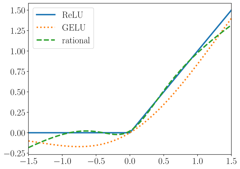
Figure 1: Comparison of three activation functions; ReLU function, GELU function [40], and rational activation function with $(r_{P},r_{Q})=(3,2)$ [41]. For rational activation function, the parameters $a_{i},b_{j}$ in Eq. (25) are initialized so that the $L^{\infty}$ distance of ReLU function and rational activation function on $[-1,1]$ is minimized.

III.3 Training the scaling function

We set up a loss function to learn the scaling function, critical temperature, and critical exponents [42]. Given Eq. (1) for a neural network with Eq. (2), we require that the scaling function satisfies the following equation for the data:

$$Y_{i}\sim\mathcal{N}[\mathsf{NN}(X_{i}),E_{i}^{2}],$$ (26)

where $X_{i},Y_{i},E_{i}$ are

$$X_{i}=(T_{i}-T_{\mathrm{c}})L_{i}^{c_{1}},$$ (27)

$$Y_{i}=L_{i}^{c_{2}}A_{i},\quad E_{i}=L_{i}^{c_{2}}\delta A_{i},$$ (28)

for $i=1,2,\dots,N$. We remark that the statistical error $E_{i}$ can vary for $X_{i}$ since physical systems that exhibit critical phenomena tend to show large data fluctuation near the critical point. The Gaussian negative log-likelihood loss function, Eq. (19), treats such data with input-dependent noises [42]. In practice, the variances $E_{i}^{2}$ is replaced with $\max(\texttt{eps},E_{i}^{2})$ with a threshold eps for computational stability, as implemented in PyTorch. We note that for homoscedastic data where $E_{i}=E$ for all $i$, the Gaussian negative log-likelihood loss function becomes the least-square regression loss function.

The goal of the learning is to find the parameter that gives the minimum value for the loss function $\mathcal{L}$. We use stochastic gradient descent methods, particularly Adam [32], to update parameters and search for optimal solutions. We summarize the tips obtained through actual experiments. The learning rate set by default in Adam’s training $\alpha=10^{-3}$ is the one recommended for training neural networks. Therefore, in learning the loss function $\mathcal{L}$ in Eq. (19), the learning rate for the parameters of the neural network and the learning rate for the critical exponents $c_{1},c_{2}$ and critical points $T_{\mathrm{c}}$, should be different so that the learning can converge in fewer iterations. In experiments, we set the learning rate for $c_{1},c_{2},T_{\mathrm{c}}$ as $\alpha_{\mathrm{c}}=10^{-2}$.

We also note how to handle the data. A typical setup for machine learning is batch learning, where the neural network weights are learned using all the data to compute the gradient. However, this method has a problem: if there is a large amount of data, the time required for each learning step becomes enormous. We usually use mini-batch learning to solve this problem, which reduces the time needed for gradient calculation by taking a subset out of the whole data set when calculating the gradient. This method is also well known to make learning less stagnant and optimization more successful. However, we confirmed that batch learning is sufficient for learning in NSA. In all of the following experiments, we used batch learning.

III.4 Clipping parameters

In many cases, the sign of the critical exponents $c_{1},c_{2}$ is known in advance when performing the FSS. Also, by the above rescaling of the temperature $T$, we know that $T_{\mathrm{c}}$ lies between $-1$ and $1$. Therefore, we need a way to optimize parameters within an interval or half-open interval. Here, unconstrained optimization is achieved by constructing a bijective map from the real number $\mathbb{R}$ to the interval. First, for optimization on the half-open interval $(a,\infty)$, we use the following bijective map:

$$y=g_{(a,\infty)}(x)\equiv\mathsf{softplus}(x)+a,$$ (29)

where $\mathsf{softplus}(x)=\log(1+e^{x})$ is another smooth approximation to the ReLU function. Second, for the half-open interval $(-\infty,a)$, we use the following bijective map:

$$y=g_{(-\infty,a)}(x)\equiv-\mathsf{softplus}(x)+a.$$ (30)

Finally, the bijective map that achieves parameter optimization on the interval $(a,b)$ is as follows:

$$y=g_{(a,b)}(x)\equiv a+(b-a)\sigma(x),$$ (31)

where $\sigma(x)=1/(1+e^{-x})$ is a sigmoid function.

All of these functions $g_{(a,\infty)},g_{(-\infty,a)},g_{(a,b)}$ are bijective maps (see Fig. 2 for the comparison), and their inverse maps are analytically calculated as follows:

$$x=g_{(a,\infty)}^{-1}(y)\equiv\log(e^{y-a}-1),$$ (32)

$$x=g_{(-\infty,a)}^{-1}(y)\equiv\log(e^{a-y}-1),$$ (33)

$$x=g_{(a,b)}^{-1}(y)\equiv\log(y-a)-\log(b-y).$$ (34)

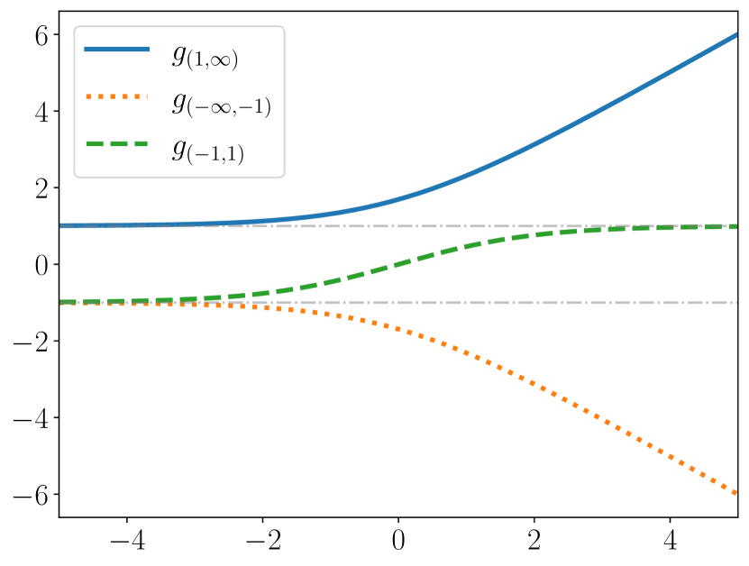
Figure 2: Comparison of three bijective maps; $g_{(1,\infty)}$, $g_{(-\infty,-1)}$, and $g_{(-1,1)}$. The gray dotted lines are the $1$ and $-1$ guidelines.

IV Numerical experiments

This section demonstrates NSA for the two-dimensional Ising model and the two-dimensional bond percolation . In both cases, we can compare the results of NSA with the exact results of those models. We discuss the performance comparison between NSA and BSA in Appendix A.

IV.1 Two-dimensional Ising model

We first consider the two-dimensional Ising model on a square lattice, where the Hamiltonian and its probability distribution are

$$\mathcal{H}(\bm{s})=-J\sum_{\langle i,j\rangle}s_{i}s_{j},$$ (35)

$$P(\bm{s})=\frac{1}{Z}\exp\left[-\mathcal{H}(\bm{s})/(k_{B}T)\right].$$ (36)

Here $s_{i}$ denotes the spin variable of the $i$th site with $s_{i}=\pm 1$, $\langle i,j\rangle$ denotes the nearest neighbor pairs, and $J$ denotes the positive coupling constant. $Z$ is the partition function, and $k_{B}$ is the Boltzmann constant. In the following, we set $J/k_{B}=1$ for simplicity. The order parameter is a magnetization defined as $M=\sum_{i}s_{i}$. The two-dimensional Ising model on a square lattice is known to be solvable [44], and the critical point is given by $\frac{1}{T_{\mathrm{c}}}=\frac{1}{2}\log(1+\sqrt{2})=0.44068\dots$, and its critical exponents are $\beta=1/8,\gamma=7/4,\nu=1$.

In this paper, we perform FSS using the Binder ratio to accurately determine the phase transition point. The Binder ratio is defined as the kurtosis of the order parameter, which reads

$$U=\frac{1}{2}\left(3-\frac{\langle M^{4}\rangle}{\langle M^{2}\rangle^{2}}\right),$$ (37)

where $\langle\cdot\rangle$ denotes the average over the canonical distribution (36). Since the Binder ratio is a dimensionless quantity and does not require scaling, its FSS form has only one critical exponent $\nu$, which reads

$$U(T,L)=\Psi_{B}[(1/T-1/T_{\mathrm{c}})L^{1/\nu}].$$ (38)

We first do the Monte Carlo simulations to obtain the Binder ratio. See [15] for the detailed settings. Now we have the dataset $\mathcal{D}=\{(1/T_{i},L_{i},U_{i},\delta U_{i})\}_{i}$, where $U_{i}$ is the $i$th Binder ratio with the inverse temperature $1/T_{i}$ and the system size $L_{i}$. $\delta U_{i}$ is the statistical error of the $i$th Binder ratio $U_{i}$. The data is shown in Fig. 3 (a) for the system size $L=64,128$ and $256$. Then to perform the NSA, we rescale the data as in Sec. III.1. The scaling function is set to a neural network with the layer size $n_{0}=n_{3}=1$ and $n_{1}=n_{2}=20$, and the loss function is set to the Gaussian negative log-likelihood function (19) with

$$X_{i}=(1/T_{i}-1/T_{\mathrm{c}})L_{i}^{c_{1}},$$ (39)

$$Y_{i}=U_{i},\quad E_{i}=\delta U_{i},$$ (40)

where the critical values are clipped with $c_{1}=g_{(0,\infty)}(\theta_{1})$ and $1/T_{\mathrm{c}}=g_{(-1,1)}(\theta_{\mathrm{c}})$.

We optimize the scaling function and $\theta_{1},\theta_{\mathrm{c}}$ with the optimizer Adam [32] for $10^{4}$ iteration times. Fig. 3 (b) shows the result of the NSA. We see that all the scaled data is on the scaling function obtained by a neural network. Fig. 4 shows the loss $\mathcal{L}$ and the critical values through $10^{4}$ iterations. We see that the loss values are well converged through iterations. The results of the critical values are $c_{1}=0.99078$ and $1/T_{\mathrm{c}}=0.44070$, which are very close to the exact results.

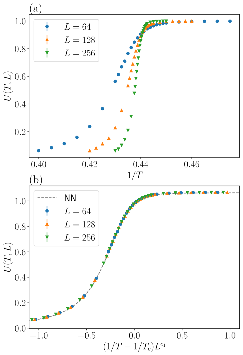
Figure 3: (a) The Binder ratios of the Ising model on a square lattice for the system size $L=64,128$ and $256$. Error bars are so small that they may not be visible. (b) Result of FSS using NSA for the Binder ratios shown in (a). The gray dashed curve shows the scaling function obtained by a neural network. We note that the data is scaled as in Sec. III.1.

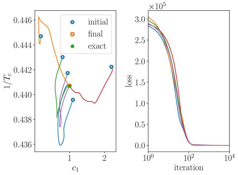
Figure 4: Critical values $(c_{1},1/T_{\mathrm{c}})$ (left) and the loss value (right) through the learning process of the Binder ratio of the two-dimensional Ising model with five different initial values.

IV.2 Two-dimensional bond percolation

Next, we demonstrate NSA for the two-dimensional bond percolation model. In percolation theory, bonds between lattice points open with probability $p$, then two points are connected. We discuss the clusters that are then formed, their size, and their dependence on the probability [45]. It is known from extensive research to date that as the probability of the opening of bonds between lattice points is increased, a phase transition phenomenon is observed in which clusters have formed that spread throughout the entire system with a certain probability $p_{\mathrm{c}}$. The value of this critical probability $p_{\mathrm{c}}$ is known for many two-dimensional lattices. See Fig. 5 for typical configurations of two-dimensional bond percolation on a square lattice with a different value of $p$ [45].

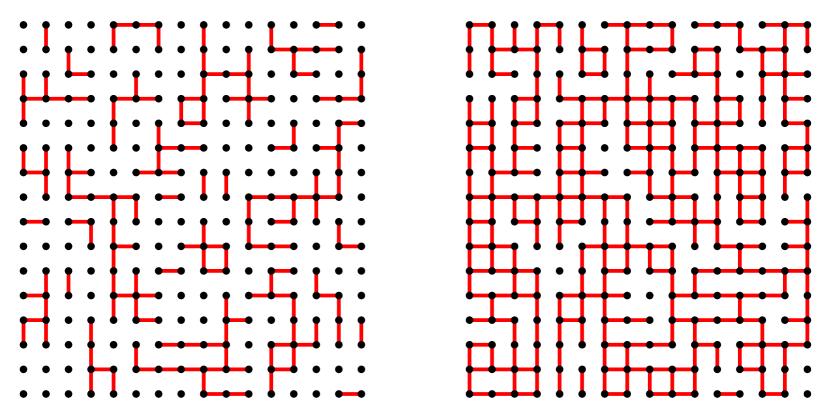
Figure 5: Typical bond percolation configurations on a square lattice with bond probabilities $p=0.3$ (left) and $p=0.6$ (right) for the lattice size $L=16$. At $p=0.3$, there are no clusters spread throughout the system. When $p=0.6$ exceeds the critical probability $p_{\mathrm{c}}=1/2$, clusters spreading throughout the system, i.e., clusters crossing up and down, or left and right, can be confirmed.

In this paper, we performed FSS using the truncated mean cluster size $\chi^{\mathrm{f}}(p)$, which is defined by the mean size of finite open clusters. By denoting the cluster containing the origin by $C$ and writing its size as $|C|$, we have

$$\chi^{\mathrm{f}}(p)=\mathbb{E}_{p}\left[|C|;|C|<\infty\right].$$ (41)

Near the critical probability $p_{\mathrm{c}}$, the truncated mean cluster size is believed to behave as $\chi^{\mathrm{f}}(p)\approx|p-p_{\mathrm{c}}|^{-\gamma}$ as $p\to p_{\mathrm{c}}$ with a critical exponent $\gamma$. Therefore its FSS form reads

$$\chi^{\mathrm{f}}(p,L)=L^{\gamma/\nu}\Phi[(p-p_{\mathrm{c}})L^{1/\nu}]$$ (42)

with a scaling function $\Phi$. For the two-dimensional bond percolation on a square lattice, the critical probability is $p_{\mathrm{c}}=1/2$, and the critical exponents are $\gamma=43/18$ and $\nu=4/3$ [45].

We note the difference between the mean cluster size $\chi(p)$ and the truncated mean cluster size $\chi^{\mathrm{f}}(p)$. The mean cluster size is defined as $\chi(p)=\mathbb{E}_{p}\left[|C|\right]$. In the subcritical phase $p<p_{\mathrm{c}}$, it is expected that $\chi(p)\approx(p_{\mathrm{c}}-p)^{-\gamma}$ for $p\uparrow p_{\mathrm{c}}$. Whereas in the supercritical phase $p>p_{\mathrm{c}}$, $\chi(p)=\infty$ from the definition of the critical probability $p_{\mathrm{c}}$, which makes $\chi(p)$ difficult to handle theoretically. For the truncated mean cluster size, it is expected that $\chi^{\mathrm{f}}(p)\approx(p-p_{\mathrm{c}})^{-\gamma^{\prime}}$ for $p\downarrow p_{\mathrm{c}}$, where we assume that $\gamma=\gamma^{\prime}$. Since $\chi(p)=\chi^{\mathrm{f}}(p)$ in the subcritical phase, the formula $\chi^{\mathrm{f}}(p)\approx|p-p_{\mathrm{c}}|^{-\gamma}$ allows us to treat both phases in a unified manner.

To perform FSS, we first do the Monte Carlo simulations to obtain the truncated mean cluster sizes. Cluster sizes can be calculated efficiently using a disjoint-set data structure and the union-find algorithm. We now have the dataset $\mathcal{D}=\{(p_{i},L_{i},\chi^{\mathrm{f}}_{i},\delta\chi^{\mathrm{f}}_{i})\}_{i}$, where $\chi^{\mathrm{f}}_{i}$ is the $i$th truncated mean cluster size with the probability $p_{i}$ and the system size $L_{i}$. $\delta\chi^{\mathrm{f}}_{i}$ is the statistical error of $\chi^{\mathrm{f}}_{i}$. The data is shown in Fig. 6 (a) for the system size $L=64,128$, and $256$ with 1000 trials. The total number of data points is 150. The rescaling of the dataset is done as in Sec. III.1, and the neural network setting is the same as the one with the two-dimensional Ising model in Sec. IV.1. The loss function is set to the Gaussian negative log-likelihood function (19) with

$$X_{i}=(p_{i}-p_{\mathrm{c}})L_{i}^{c_{1}},$$ (43)

$$Y_{i}=L_{i}^{c_{2}}\chi^{\mathrm{f}}_{i},\quad E_{i}=L_{i}^{c_{2}}\delta\chi^{\mathrm{f}}_{i},$$ (44)

where the critical values are clipped with $c_{1}=g_{(0,\infty)}(\theta_{1})$, $c_{2}=g_{(-\infty,0)}(\theta_{2})$, and $p_{\mathrm{c}}=g_{(-1,1)}(\theta_{\mathrm{c}})$. The exact values of two-dimensional bond percolation problem are $p_{\mathrm{c}}=1/2=0.5,c_{1}=3/4=0.75,c_{2}=-43/24=-1.7916\dots$. By optimizing the loss function with the Adam optimizer, we have successfully obtained the critical probability $p_{\mathrm{c}}=0.5002$ and the critical exponents $c_{1}=0.7540,c_{2}=-1.763$. Fig. 7 shows the loss $\mathcal{L}$ and the critical values through $10^{4}$ iterations. In Fig. 6 (b), we see that the scaled data are collapsed on a single curve, and the trained neural network is well approximated to the scaling function.

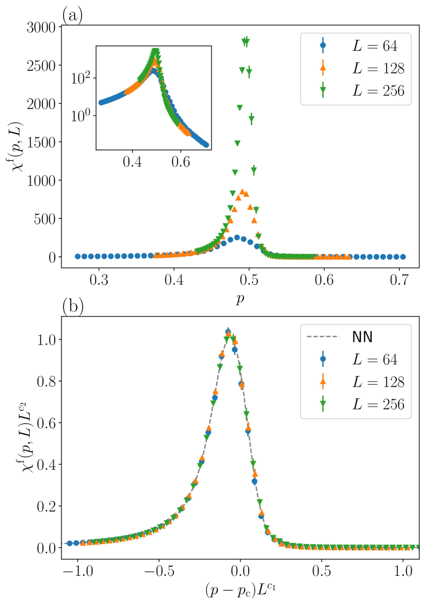
Figure 6: (a) The truncated mean cluster sizes $\chi^{\mathrm{f}}(p,L)$ of the bond percolation on a two-dimensional square lattice for the system size $L=64,128$ and $256$. Each point is the result of 1000 trials. Error bars are so small that they may not be visible. The inset shows the $\log$ scale of $\chi^{\mathrm{f}}(p,L)$. (b) Result of FSS using NSA for the truncated mean cluster sizes shown in (a). The gray dashed curve shows the scaling function obtained by a neural network. We note that the data is scaled as in Sec. III.1.

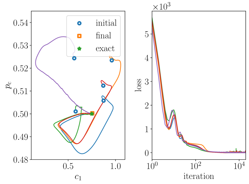
Figure 7: Critical values $(c_{1},p_{\mathrm{c}})$ (left) and the loss value (right) through the learning process of the truncated mean cluster size of the two-dimensional bond percolation model with five differential initial values.

V Accuracy of the estimation of critical values

In the previous section, we confirmed that the critical values could be estimated using a neural network based on numerical data of critical phenomena. However, this is only one estimation result, and we do not know how much we can trust this result. Most studies that numerically determine the critical value provide confidence intervals for its value. How should we calculate the confidence interval by the NSA proposed in this paper?

Here, we consider using a bootstrap-like approach to calculate confidence intervals for critical values [46]. The bootstrap approach is based on the following procedure: First, we randomly resample the data of the critical phenomena with replacement. Next, we take random initial values for the parameters learned in the NSA. The weights of the neural network are initialized randomly as described in Sec. II.2, and the parameters of the critical values $c_{1},c_{2},T_{\mathrm{c}}$ are chosen uniformly at random from the appropriate interval, respectively. Using the dataset and the initial values of the parameters prepared in this way, we obtain the critical values by NSA. We perform these procedures several times and calculate the standard deviation for a series of critical values, setting this as a $1\sigma$ confidence interval for the critical values.

For example, let us determine the confidence interval of the critical values of the two-dimensional bond percolation model. We use the truncated mean cluster size $\chi^{\mathrm{f}}$ used in Sec. IV.2 as our data. For the initial values of the critical values $p_{\mathrm{c}},c_{1}$, and $c_{2}$, we choose uniformly at random from intervals $[0.432,0.583],[0.6,0.9]$, and $[-1.9,-1.6]$, respectively. Under this configuration, we calculate the critical values 500 times and obtain the confidence interval. In Fig. 8, we use the truncated mean cluster size for the data with system size triplets $L=64,128,256$ and $L=512,1024,2048$. We vary the total data size from 100 to 600 and plot the learned critical values with $1\sigma$ confidence intervals. As can be seen in the figure, the error bar becomes smaller as the data size increases, indicating that we get a more accurate result for a larger number of data for the two-dimensional percolation model. We also observe that for $p_{\mathrm{c}}$ and $c_{1}$, the accuracy with respect to the true value improves as the system size $L$ of the data used for training is increased.

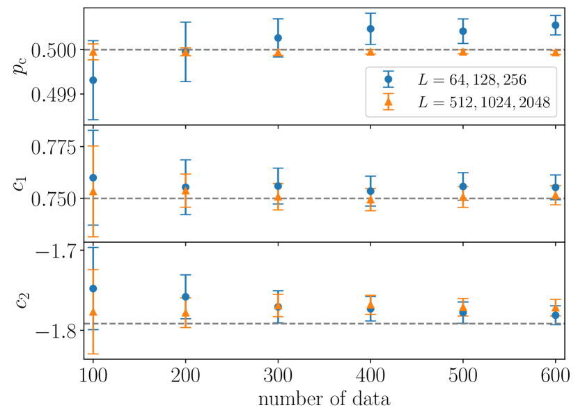
Figure 8: Learned critical values $c_{1},c_{2}$ and the critical point $p_{\mathrm{c}}$ for the two-dimensional bond percolation model with confidence intervals indicated by error bars. We vary the total number of data from 100 to 600. Blue circle points represent the system size triplet $L=64,128,256$, and orange triangle points represent the system size triplet $L=512,1024,2048$. Confidence intervals are calculated by the bootstrap approach with 500 resamplings. True values are plotted with gray dashed lines.

VI Conclusions and discussion

We proposed a method for the scaling analysis of critical phenomena using neural networks. The basic idea of this method is to model the scaling function by a neural network. For example, we consider FSS analysis, but we can apply it to general scaling analysis, which contains an unknown scaling function. The method is computationally lighter than the previously proposed method for scaling analysis using GP regression, making it a simpler method.

We demonstrate it for the two-dimensional Ising and bond percolation models. We could accurately obtain the critical points and exponents, and the data are well-collapsed to the learned scaling function for both cases. Because the computational complexity is linear for the number of data points, we can handle the FSS analysis efficiently.

Using a bootstrap-like approach, we also check the robustness of the estimation results of the new method and define the confidential intervals as the standard deviation of estimated values. They are consistent with the exact values. Another approach to determine the accuracy of the critical values would be to use the stochastic gradient Langevin dynamics [47], which achieves the Bayesian learning by adding noise to the gradient method. It has the advantage of being a Bayesian approach but scales linearly in computational complexity for the number of data.

Appendix A Comparison between NSA and BSA

In this section, we compare the performance of NSA and BSA, particularly with respect to computation time and accuracy of critical values.

A.1 Computation time

Let us compare the execution time by NSA with BSA with respect to the number of data. PyTorch and JAX implementations were used to execute NSA. PyTorch implementation was used to execute BSA. The execution environment is as follows: [OS] macOS 12.5.1, [CPU] Apple M1 Max, [Memory] 32GB. In Fig. 9, we measured the (average) computation time per epoch for NSA and BSA and plotted how much the computation time increases as the number of data increases, taking the case with 100 data as 1. As can be seen, the computation time of NSA is linear to the number of data, while BSA shows a larger growth rate of computation time with respect to the number of data. This is because BSA requires $O(N^{3})$ computational complexity due to inverse matrix calculation, while NSA requires only linear $O(N)$ computational complexity. We note that the JAX implementation uses jax.jit(), which performs just in time (JIT) compilation [48, 49], so it allows for faster execution than PyTorch.

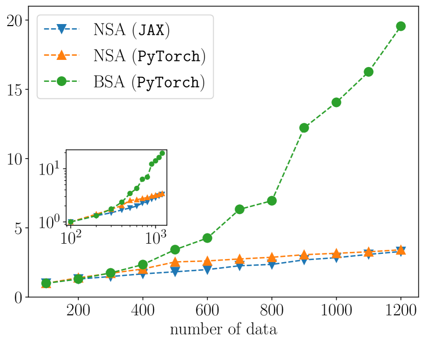
Figure 9: Relative average execution time for one epoch where we scale the execution time for 100 data as 1. The data used is the truncated mean cluster size of the two-dimensional bond percolation. The inset shows the log-log plot.

A.2 Accuracy of critical values

We next calculate the confidence intervals of critical values for the two-dimensional Ising model and compare the accuracy of NSA and BSA methods. For data used in Sec. IV.1, we resample the data with replacement and calculate the critical values for 500 times. Figure 10 shows the results of bootstrap for NSA and BSA. We observe that the learned results are more concentrated in the NSA compared to the BSA. For the BSA method, $c_{1}=0.989(5)$ and $1/T_{\mathrm{c}}=0.44071(3)$, whereas for the NSA method, $c_{1}=0.991(2)$ and $1/T_{\mathrm{c}}=0.44070(1)$.

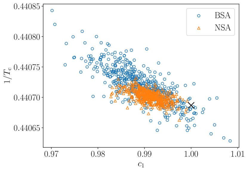
Figure 10: Final learned value distributions of critical values $(c_{1},1/T_{\mathrm{c}})$ for NSA and BSA for two-dimensional Ising model. The cross mark represents the theoretical value $c_{1}=1$ and $1/T_{\mathrm{c}}=\frac{1}{2}\log(1+\sqrt{2})$

References

- Wilson [1971a] K. G. Wilson, Renormalization Group and Critical Phenomena. I. Renormalization Group and the Kadanoff Scaling Picture, Physical Review B 4, 3174 (1971a).
- Wilson [1971b] K. G. Wilson, Renormalization Group and Critical Phenomena. II. Phase-Space Cell Analysis of Critical Behavior, Physical Review B 4, 3184 (1971b).
- Wilson and Kogut [1974] K. G. Wilson and J. Kogut, The renormalization group and the expansion, Physics Reports 12, 75 (1974).
- Wilson [1983] K. G. Wilson, The renormalization group and critical phenomena, Reviews of Modern Physics 55, 583 (1983).
- Goldenfeld [2018] N. Goldenfeld, Lectures on phase transitions and the renormalization group (CRC Press, 2018).
- Cardy [1996] J. Cardy, Scaling and renormalization in statistical physics, Vol. 5 (Cambridge university press, 1996).
- Henkel et al. [2008] M. Henkel, H. Hinrichsen, S. Lübeck, and M. Pleimling, Non-equilibrium phase transitions, Vol. 1 (Springer, 2008).
- Cardy [2012] J. Cardy, Finite-size scaling (Elsevier, 2012).
- Binder [1981] K. Binder, Finite size scaling analysis of ising model block distribution functions, Zeitschrift für Physik B Condensed Matter 43, 119 (1981).
- Slevin and Ohtsuki [1999] K. Slevin and T. Ohtsuki, Corrections to scaling at the Anderson transition, Physical Review Letters 82, 382 (1999).
- Wang et al. [2006] L. Wang, K. Beach, and A. W. Sandvik, High-precision finite-size scaling analysis of the quantum-critical point of Heisenberg antiferromagnetic bilayers, Physical Review B 73, 014431 (2006).
- Harada et al. [2013] K. Harada, T. Suzuki, T. Okubo, H. Matsuo, J. Lou, H. Watanabe, S. Todo, and N. Kawashima, Possibility of deconfined criticality in Heisenberg models at small , Physical Review B 88, 220408 (2013).
- Otsuka et al. [2016] Y. Otsuka, S. Yunoki, and S. Sorella, Universal quantum criticality in the metal-insulator transition of two-dimensional interacting Dirac electrons, Physical Review X 6, 011029 (2016).
- Yoneda et al. [2020] R. Yoneda, K. Harada, and Y. Y. Yamaguchi, Critical exponents in coupled phase-oscillator models on small-world networks, Physical Review E 102, 062212 (2020).
- Harada [2011] K. Harada, Bayesian inference in the scaling analysis of critical phenomena, Physical Review E 84, 056704 (2011).
- Harada [2015] K. Harada, Kernel method for corrections to scaling, Physical Review E 92, 012106 (2015).
- Williams and Rasmussen [2006] C. K. Williams and C. E. Rasmussen, Gaussian processes for machine learning, Vol. 2 (MIT press Cambridge, MA, 2006).
- Nasu and Motome [2015] J. Nasu and Y. Motome, Thermodynamics of chiral spin liquids with abelian and non-abelian anyons, Physical Review Letters 115, 087203 (2015).
- Singh et al. [2016] R. Singh, J. H. Bardarson, and F. Pollmann, Signatures of the many-body localization transition in the dynamics of entanglement and bipartite fluctuations, New Journal of Physics 18, 023046 (2016).
- Hesselmann and Wessel [2016] S. Hesselmann and S. Wessel, Thermal Ising transitions in the vicinity of two-dimensional quantum critical points, Physical Review B 93, 155157 (2016).
- D’Emidio and Kaul [2017] J. D’Emidio and R. K. Kaul, New Easy-Plane Fixed Points, Physical Review Letters 118, 187202 (2017).
- Horita et al. [2017] T. Horita, H. Suwa, and S. Todo, Upper and lower critical decay exponents of Ising ferromagnets with long-range interaction, Physical Review E 95, 012143 (2017).
- Ferrari et al. [2017] F. Ferrari, S. Bieri, and F. Becca, Competition between spin liquids and valence-bond order in the frustrated spin-1/2 Heisenberg model on the honeycomb lattice, Physical Review B 96, 104401 (2017).
- Iino et al. [2019] S. Iino, S. Morita, N. Kawashima, and A. W. Sandvik, Detecting signals of weakly first-order phase transitions in two-dimensional Potts models, Journal of the Physical Society of Japan 88, 034006 (2019).
- Lang and Läuchli [2019] T. C. Lang and A. M. Läuchli, Quantum Monte Carlo simulation of the chiral Heisenberg Gross-Neveu-Yukawa phase transition with a single Dirac cone, Physical Review Letters 123, 137602 (2019).
- Nomura and Imada [2021] Y. Nomura and M. Imada, Dirac-type nodal spin liquid revealed by refined quantum many-body solver using neural-network wave function, correlation ratio, and level spectroscopy, Physical Review X 11, 031034 (2021).
- Goodfellow et al. [2016] I. Goodfellow, Y. Bengio, and A. Courville, Deep Learning (MIT Press, Cambridge, Massachusetts, 2016).
- Carleo et al. [2019] G. Carleo, I. Cirac, K. Cranmer, L. Daudet, M. Schuld, N. Tishby, L. Vogt-Maranto, and L. Zdeborová, Machine learning and the physical sciences, Reviews of Modern Physics 91, 045002 (2019).
- Wang [2016] L. Wang, Discovering phase transitions with unsupervised learning, Phys. Rev. B 94, 195105 (2016).
- Ohtsuki and Ohtsuki [2016] T. Ohtsuki and T. Ohtsuki, Deep learning the quantum phase transitions in random two-dimensional electron systems, Journal of the Physical Society of Japan 85, 123706 (2016).
- Carrasquilla and Melko [2017] J. Carrasquilla and R. G. Melko, Machine learning phases of matter, Nature Physics 13, 431 (2017).
- Kingma and Ba [2017] D. P. Kingma and J. Ba, Adam: A method for stochastic optimization (2017), arXiv:1412.6980 [cs.LG] .
- Kanagawa et al. [2018] M. Kanagawa, P. Hennig, D. Sejdinovic, and B. K. Sriperumbudur, Gaussian processes and kernel methods: A review on connections and equivalences (2018), arXiv:1807.02582 [stat.ML] .
- Cybenko [1989] G. Cybenko, Approximation by superpositions of a sigmoidal function, Mathematics of Control, Signals and Systems 2, 303 (1989).
- Hornik [1991] K. Hornik, Approximation capabilities of multilayer feedforward networks, Neural networks 4, 251 (1991).
- Ruder [2016] S. Ruder, An overview of gradient descent optimization algorithms (2016).
- Baydin et al. [2015] A. G. Baydin, B. A. Pearlmutter, A. A. Radul, and J. M. Siskind, Automatic differentiation in machine learning: a survey (2015).
- Bradbury et al. [2018] J. Bradbury, R. Frostig, P. Hawkins, M. J. Johnson, C. Leary, D. Maclaurin, G. Necula, A. Paszke, J. VanderPlas, S. Wanderman-Milne, and Q. Zhang, JAX: composable transformations of Python+NumPy programs (2018).
- Paszke et al. [2019] A. Paszke, S. Gross, F. Massa, A. Lerer, J. Bradbury, G. Chanan, T. Killeen, Z. Lin, N. Gimelshein, L. Antiga, A. Desmaison, A. Kopf, E. Yang, Z. DeVito, M. Raison, A. Tejani, S. Chilamkurthy, B. Steiner, L. Fang, J. Bai, and S. Chintala, PyTorch: An Imperative Style, High-Performance Deep Learning Library, in Advances in Neural Information Processing Systems 32, edited by H. Wallach, H. Larochelle, A. Beygelzimer, F. d'Alché-Buc, E. Fox, and R. Garnett (Curran Associates, Inc., 2019) pp. 8024–8035.
- Hendrycks and Gimpel [2020] D. Hendrycks and K. Gimpel, Gaussian error linear units (GELUs) (2020), arXiv:1606.08415 [cs.LG] .
- Boullé et al. [2020] N. Boullé, Y. Nakatsukasa, and A. Townsend, Rational neural networks, in Advances in Neural Information Processing Systems, Vol. 33 (2020) pp. 14243–14253.
- Nix and Weigend [1994] D. Nix and A. Weigend, Estimating the mean and variance of the target probability distribution, in Proceedings of 1994 IEEE International Conference on Neural Networks (ICNN'94) (IEEE, 1994).
- Note [1] The code implemented in Python is available on GitHub together with the dataset: JAX implementation (https://github.com/yonesuke/jaxfss) and PyTorch implementation (https://github.com/KenjiHarada/FSS-tools).
- Baxter [2007] R. Baxter, Exactly solved models in statistical mechanics (Dover Publications, Mineola, N.Y, 2007).
- Grimmett [1999] G. Grimmett, Percolation (Springer Berlin Heidelberg, 1999).
- Efron [1992] B. Efron, Bootstrap methods: another look at the jackknife, in Breakthroughs in statistics (Springer, 1992) pp. 569–593.
- Welling and Teh [2011] M. Welling and Y. W. Teh, Bayesian learning via stochastic gradient Langevin dynamics, in Proceedings of the 28th international conference on machine learning (ICML-11) (Citeseer, 2011) pp. 681–688.
- [48] Just In Time Compilation with JAX, https://jax.readthedocs.io/en/latest/jax-101/02-jitting.html, accessed: 2022-09-02.
- tf [2] XLA: Optimizing Compiler for Machine Learning, https://www.tensorflow.org/xla, accessed: 2022-09-02.