Learning from a Biased Sample

Abstract

The empirical risk minimization approach to data-driven decision making assumes that we can learn a decision rule from training data drawn under the same conditions as the ones we want to deploy it in. However, in a number of settings, we may be concerned that our training sample is biased, and that some groups (characterized by either observable or unobservable attributes) may be under- or over-represented relative to the general population; and in this setting empirical risk minimization over the training set may fail to yield rules that perform well at deployment. We propose a model of sampling bias called $\Gamma$-biased sampling, where observed covariates can affect the probability of sample selection arbitrarily much but the amount of unexplained variation in the probability of sample selection is bounded by a constant factor. Applying the distributionally robust optimization framework, we propose a method for learning a decision rule that minimizes the worst-case risk incurred under a family of test distributions that can generate the training distribution under $\Gamma$-biased sampling. We apply a result of Rockafellar and Uryasev to show that this problem is equivalent to an augmented convex risk minimization problem. We give statistical guarantees for learning a model that is robust to sampling bias via the method of sieves, and propose a deep learning algorithm whose loss function captures our robust learning target. We empirically validate our proposed method in simulations and a case study on ICU length of stay prediction.

1 Introduction

Empirical risk minimization is a practical and popular approach to learning data-driven decision rules (Bertsimas and Kallus, 2020; Kitagawa and Tetenov, 2018; Vapnik, 1995). Formally, suppose that we observe $i=1,\,\ldots,\,n$ samples $(X_{i},Y_{i})$ independently drawn from a distribution $P$, where $X\in\mathcal{X}$ are covariates and $Y\in\mathcal{Y}$ is a target outcome, and we want to learn a decision rule $h$ that minimizes a loss $L$ under $P$:

$$h^{*}=\operatorname*{argmin}_{h}\mathbb{E}_{(X,\,Y)\sim P}\left[L(h(X),Y)\right].$$ (1)

Then, empirical risk minimization involves choosing a decision rule $\hat{h}$ that is a (potentially penalized) minimizer of the in-sample loss $n^{-1}\sum_{i=1}^{n}L(h(X_{i}),\,Y_{i})$; and the learned decision rule is deemed to perform well if the loss of $\hat{h}$ approaches the minimum possible loss that could be attained using $h^{*}$ (Vapnik, 1995).

Formal justifications for empirical risk minimization crucially rely on the assumption that the target distribution we want to deploy our decision rule on, i.e., the one used to define the objective in (1), is the same as the distribution $P$ from which we drew the training samples $(X_{i},\,Y_{i})$ used for learning. In several important application areas, however, sampling bias in the data collection process may prevent practitioners from accessing training data from the distribution that they intend to deploy the rule on; and such sampling bias may hurt the target distribution performance of decision rules learned via empirical risk minimization.

One setting where sampling bias can be a concern is in designing risk predictors in a medical setting. Various risk predictors are widely used to guide both clinical practice and hospital logistics: Goff et al. (2014) discuss how risk predictors for cardiovascular disease are used to inform clinical guidelines, while Gul and Celik (2020) present a number of approaches to predicting emergency room admissions that can be used to anticipate hospital staffing needs. We may be concerned about sampling bias if these risk models are trained using data from a handful of hospitals (e.g., university hospitals participating in a study), and if the patients in these hospitals are not representative of the general patient population.

Another major situation where sampling bias may matter is in studies run on volunteers. In randomized trials for estimating treatment effects, participants often volunteer or apply to be a part of the study: Attanasio et al. (2011) measures the effect of a vocational training program on labor market outcomes in a randomized trial where participants needed to apply to be a part of the study; and the effectiveness of antidepressants is typically assessed in randomized trials involving volunteers (Wang et al., 2018). In such studies, participants may differ from non-participants in fundamental ways, and a decision rule based on trial data may perform poorly when deployed on non-participants. Furthermore, vulnerable populations may be less exposed to study recruitment, so failure to generalize under sampling bias may cause these populations to be disproportionately impacted by errors of the decision rule.

The goal of this paper is to develop an alternative to empirical risk minimization that is robust to potential sampling bias. We still assume that we get to work with $n$ i.i.d. samples from $P$; however, we now define the optimal decision rule in terms of a different distribution $Q$,

$$h^{*}=\operatorname*{argmin}_{h}\mathbb{E}_{(X,\,Y)\sim Q}\left[L(h(X),Y)\right],$$ (2)

and allow for the prospect that $P$ may be biased relative to our target distribution $Q$. For example, in the context of medical risk prediction, $Q$ could be the nationwide patient distribution, whereas $P$ is the patient distribution in the hospitals we have data from.

Of course, if there is no link between our sampling distribution $P$ and our target distribution $Q$, then learning data-driven rules is not possible. Throughout this paper, we will assume that $P$ is biased—but not too biased—relative to $Q$, in the sense formalized by the $\Gamma$-biased sampling model given below. Here, $\Gamma\geq 1$ captures the allowed strength of sampling bias, and larger values of $\Gamma$ allow for more bias.

Definition 1.

Let $\Gamma\geq 1$. For any pair of distributions $P$ and $Q$ over $(X,Y)$, we say that $Q$ can generate $P$ under $\Gamma$-biased sampling if there exists a distribution $\tilde{Q}$ over $(X,Y,S)$, where $S\in\{0,1\}$ is a “selection indicator” that satisfies the following properties: The $(X,Y)$-marginal of $\tilde{Q}$ is equal to $Q$, then $(X,Y)$-marginal of $\tilde{Q}$ conditionally on $S=1$ is equal to $P$, and

$$\frac{\mathbb{P}_{\tilde{Q}}\left[S=1\mid X=x,Y=y\right]}{\mathbb{P}_{\tilde{Q}}\left[S=1\mid X=x\right]}\in[\Gamma^{-1},\Gamma]\quad\forall x\in\mathcal{X},y\in\mathcal{Y}.$$ (3)

This model of sampling bias is an extension of the model adopted in Aronow and Lee (2013) and Miratrix et al. (2018) to the setting where there are covariates $X$ that may affect whether a sample is selected $(S=1)$. In $\Gamma$-biased sampling, the covariates $X$ may affect the probability of sample selection arbitrarily much, but the amount of unexplained variation in the probability of sample selection is limited due to (3). On the other hand, the model with $\Gamma=1$ corresponds to “unconfounded sample selection” that is widely studied in the literature on generalizability (e.g., Stuart et al., 2011; Tipton, 2013, 2014).

One challenge of learning under $\Gamma$-biased sampling is that the true test distribution is unknown and there are many possible distributions that can generate the observed training distribution $P$ under $\Gamma$-biased sampling. To address this problem, we use distributionally robust optimization (DRO) (Ben-Tal et al., 2013) to learn a decision rule that is robust to all distributions that can generate our observed training distribution $P$ under $\Gamma$-biased sampling. The goal of DRO is to minimize the worst-case risk over a family of plausible test distributions $\mathcal{S}$ (the robustness set), i.e.

$$\operatorname*{argmin}_{h}\sup_{Q\in\mathcal{S}}\mathbb{E}_{Q}\left[L(h(X),Y)\right].$$ (4)

To learn decision rules that are robust to $\Gamma$-biased sampling, we consider robustness sets $\mathcal{S}_{\Gamma}(P,Q_{X})$ for $\Gamma>1$, where $Q\in\mathcal{S}_{\Gamma}(P,Q_{X})$ if $Q$ can generate $P$ via $\Gamma$-biased sampling and $Q$ has covariate distribution equal to $Q_{X}$.

The main contribution of this work is a method for learning

$$h^{*}_{\Gamma}=\operatorname*{argmin}_{h}\sup_{Q\in\mathcal{S}_{\Gamma}(P,Q_{X})}\mathbb{E}_{Q}\left[L(h(X),Y)\right]$$ (5)

for any distribution $Q_{X}$ that is absolutely continuous to $P_{X}$. We show that there is a convex loss function $L_{\text{RU}}^{\Gamma}$ (given below), defined over an augmented feature space, such that the solution to the following risk minimization problem

$$\begin{split}&(h^{*}_{\Gamma},\alpha^{*}_{\Gamma})=\operatorname*{argmin}_{h,\alpha}\mathbb{E}_{P}\left[L_{\text{RU}}^{\Gamma}(h(X),\alpha(X),Y)\right],\\ &L_{\text{RU}}^{\Gamma}(z,a,y)=\Gamma^{-1}L(z,y)+(1-\Gamma^{-1})a+(\Gamma-\Gamma^{-1})(L(z,\,y)-a)_{+},\end{split}$$ (6)

with data drawn from the training distribution $P$, also solves (5) for any distribution $Q_{X}$ that is absolutely continuous with respect to $P_{X}$. We call the minimization problem in (6) Rockafellar-Uryasev (RU) Regression and $L_{\text{RU}}^{\Gamma}$ the RU loss because results of Rockafellar and Uryasev (2000) play a key role in our derivation of this loss function. A notable aspect of our proposed method is that it does not require any knowledge of $Q_{X}$ because it relies on the fact that the minimization of the worst-case risk over a sufficiently flexible class of functions is equivalent to minimization of the conditional worst-case risk for every $x\in\mathcal{X}.$

The remainder of the paper investigates RU Regression theoretically and empirically. In Section 3.1, we demonstrate useful properties of the population RU risk, including convexity, differentiability, existence and uniqueness of the minimizer, and strong convexity around the minimizer. In Section 3.2, these properties enable us to derive formal guarantees for learning via empirical minimization of $L_{\text{RU}}^{\Gamma}$ using the method of sieves (Geman and Hwang, 1982). Furthermore, the useful properties of the population RU risk also suggest that for practical implementation, the problem in (6) can be solved via stochastic gradient descent. As a result, we propose to perform the optimization in (6) by joint-training of neural networks, one for each of $h$ and $\alpha$, with the RU loss as the objective. In Section 4, we validate our approach in simulations and a case study with the MIMIC-III dataset (Johnson et al., 2016a).

1.1 Related Work

Our proposed model of sampling bias, $\Gamma$-biased sampling, builds on previous models for sampling bias (Aronow and Lee, 2013; Miratrix et al., 2018), where samples $Y_{i}$ are drawn i.i.d. from the target distribution $Q$ but only included in the training dataset with a latent probability $\pi_{i}\in[\alpha,\beta]$, for $\alpha,\beta\in(0,1]$. Under this model, these works focus on partial identification of the population mean outcome $\mathbb{E}_{Q}\left[Y\right]$. If we interpret $\pi_{i}:=\mathbb{P}_{\tilde{Q}}\left[S_{i}\,\big{|}\,X_{i},\,Y_{i}\right]$, then our $\Gamma$-biased sampling model as specified in Definition 1 is statistically equivalent to an extension of the model used in Aronow and Lee (2013) and Miratrix et al. (2018) to include covariates, in such a way that we allow the unobserved probability of sample selection $\pi$ to be arbitrarily affected by the covariates $X$ but place bounds on the amount of unexplained variation in $\pi_{i}$. Also, unlike Aronow and Lee (2013) and Miratrix et al. (2018), we focus on the problem of learning a robust decision rule rather than on partial identification of moments of $Q$.

Our model is also connected to the broader literature on sensitivity analysis in causal inference (Andrews and Oster, 2019; Dorn et al., 2021; Jin et al., 2022; Nie et al., 2021; Yadlowsky et al., 2018), the goal of which is to understand how causal analyses justified by assuming randomized or unconfounded treatment assignment could be affected by a failure of these assumptions. In particular, our $\Gamma$-biased sampling model has a similar statistical structure as the $\Gamma$-marginal sensitivity model used by Tan (2006) to quantify failures of unconfoundedness. However, in these sensitivity analyses, the concern is typically regarding threats to internal validity (i.e., failures of unconfoundedness), whereas here we model sampling bias as a threat to external validity.

To learn a decision rule that is robust to $\Gamma$-biased sampling, we apply the DRO framework, which is widely used for learning models that are robust to unknown distribution shift (Duchi and Namkoong, 2021; Duchi et al., 2020; Hu et al., 2018; Michel et al., 2022; Mohajerin Esfahani and Kuhn, 2018; Oberst et al., 2021; Oren et al., 2019; Sagawa et al., 2019; Thams et al., 2022). Previous works that apply DRO for learning robust models typically specify a robustness set of interest and provide a method for either evaluating the worst-case risk over the set, learning the solution that minimizes the worst-case risk over the set, or both. These works vary in how they define the robustness set and whether they consider robustness sets over the conditional distribution of $Y$ given $X$, the marginal distribution over $X$, or the joint distribution over $(X,Y)$. While learning under our $\Gamma$-sampling bias model is conceptually a DRO problem, our problem setting has many crucial differences from the most widely studied DRO setting, e.g., the one considered in Duchi et al. (2020); and these differences require us to develop new learning algorithms and new analysis techniques to prove formal results. We discuss connections to the DRO literature in more detail in Section 2.2.

Finally, our contribution is related to the broader literature on data-driven decision making. This literature has been active in recent years, including contributions from Athey and Wager (2021), Bertsimas and Kallus (2020), Elmachtoub and Grigas (2022), Foster and Syrgkanis (2019), Kallus and Zhou (2021), Kitagawa and Tetenov (2018), Manski (2004), Nie and Wager (2021), Stoye (2009), Swaminathan and Joachims (2015), Zhao et al. (2012) and Zhou et al. (2022). A recurring theme of this line of work is in choosing loss functions $L(\cdot)$ that capture relevant aspects of various decision tasks (Bertsimas and Kallus, 2020). Our results pair naturally with this line of work, in that our approach can be applied with generic loss functions to learn decision rules that are robust to potential sampling bias. We also draw attention to Kallus and Zhou (2021), who consider learning optimal treatment rules from confounded data, i.e., where the “treated” and “control” samples available for training may be biased according to unobservable attributes. Our work is related to that of Kallus and Zhou (2021) in that we both consider using robust optimization techniques to learn from data potentially corrupted via biased sampling; however, the type of bias we consider (test/train vs. treatment/control), and resulting algorithmic and conceptual remedies, are different.

2 Rockafellar-Uryasev Regression

We consider the following general loss minimization setting. We have access to $i=1,\,\ldots,\,n$ samples $(X_{i},\,Y_{i})$ drawn from a training distribution $P$ over $\mathcal{X}\times\mathcal{Y}$. We seek to learn a decision rule $h$ such that, given a loss function $L(z,y)$, the expected loss $\mathbb{E}_{Q}\left[L(h(X),\,Y)\right]$ is small when $(X,\,Y)$ is drawn from our target distribution $Q$. The key challenge is that we do not assume that the training distribution $P$ and the target $Q$ are the same. Rather, $Q$ is unknown, and we only assume that $Q$ generates $P$ via $\Gamma$-biased sampling in the sense of Definition 1, for some $\Gamma\geq 1$.

For any marginal covariate distribution $Q_{X}$, let $S_{\Gamma}(P,\,Q_{X})$ denote the set of all distributions $Q$ are related to $P$ via $\Gamma$-biased sampling and have marginal distribution over $X$ equal to $Q_{X}$. (Recall that Definition 1 only bounds “unexplained” sampling bias allows; it allows for arbitrary sampling bias explained by $X$, and thus places no meaningful restrictions on $Q_{X}$). Given any choice of $Q_{X}$, we target the robust decision rule

$$h^{*}_{Q_{X},\,\Gamma}\in\operatorname*{argmin}_{h\in L^{2}(P_{X},\,\mathcal{X})}\sup\Big{\{}\mathbb{E}_{Q}\left[L(h(X),\,Y)\right]:Q\in S_{\Gamma}(P,\,Q_{X})\Big{\}},$$ (7)

where $L^{2}(P_{X},\,\mathcal{X})$ denotes the space of square-integrable measurable functions with respect to $P_{X}$. The formulation (7) may look challenging to use as the basis for a practical approach to learning. First, it is formulated in terms of the marginal distribution $Q_{X}$ which may sometimes be known (e.g., Nie et al., 2021), but often is not known. Second, the optimization problem (7) has a min-max form that is not obviously amenable to statistical learning. The following results show how both of these challenges can be addressed.

As a preliminary to our subsequent analysis, we start by giving a more explicit characterization of the set $\mathcal{S}_{\Gamma}(P,Q_{X})$ that can generate $P$ under $\Gamma$-based sampling: $Q$ can generate $P$ via $\Gamma$-biased sampling if and only if the likelihood ratio between the conditional distributions of $Y\mid X$ of $Q$ and $P$ is bounded between $\Gamma^{-1}$ and $\Gamma$ and the density ratio between the covariate distributions of $P$ and $Q$ are bounded.

Lemma 1.

Let $P,Q$ be the distributions over $(X,Y)$. $Q$ can generate $P$ via $\Gamma$-biased sampling if and only if

$$\Gamma^{-1}\leq\frac{dQ_{Y\mid X=x}(y)}{dP_{Y\mid X=x}(y)}\leq\Gamma,\quad\forall x\in\mathcal{X},y\in\mathcal{Y}$$ (8)

and $\sup_{x\in\mathcal{X}}\frac{dP_{X}(x)}{dQ_{X}(x)}<C$ for some $C<\infty$. Proof in Appendix C.3.

We are now ready to spell out our first main result, i.e., a reformulation of our learning objective (7) as the minimizer of the expectation a convex function over data drawn from the training distribution $P$. We demonstrate that there exists a single function $h^{*}_{\Gamma}$ that solves the problem (7) simultaneously for any $Q_{X}$ that is absolutely continuous with respect to $P_{X}$, and furthermore this $h^{*}_{\Gamma}$ can be characterized as the minimizer of a convex loss defined in terms of the observed data distribution $P$. We refer to the loss function in (9) the Rockafellar-Uryasev (RU) loss because the proof of Theorem 2 draws heavily from results of Rockafellar and Uryasev (2000); we will also refer to learning via empirical minimization based on (9) as RU Regression.

Theorem 2.

Suppose that $(X,\,Y)\in\mathcal{X}\times\mathcal{Y}$ are drawn i.i.d. with respect to a distribution $P$ for some $\mathcal{X}\subseteq\mathbb{R}^{d}$ and $Y\subseteq\mathbb{R}$. Let $L(z,\,y)$ be a loss function that is convex in $z$ for any $y\in\mathcal{Y}$, and let $\Gamma>1$. Then the following augmented loss function,

$$L_{\text{RU}}^{\Gamma}(z,a,y)=\Gamma^{-1}L(z,y)+(1-\Gamma^{-1})a+(\Gamma-\Gamma^{-1})(L(z,\,y)-a)_{+},$$ (9)

is convex is $(z,\,a)$ for any $y\in\mathcal{Y}$. Furthermore, any solution

$$\{h^{*}_{\Gamma},\,\alpha^{*}_{\Gamma}\}\in\operatorname*{argmin}_{(h,\,\alpha)\in L^{2}(P_{X},\,\mathcal{X})\times L^{2}(P_{X},\,\mathcal{X})}\mathbb{E}_{P}\left[L_{\text{RU}}^{\Gamma}(h(X),\,\alpha(X),\,Y)\right]$$ (10)

is also a solution to (7) for any $Q_{X}$ that is absolutely continuous with respect to $P_{X}$, i.e., $Q_{X}\ll P_{X}$ and $\sup_{x\in\mathcal{X}}\frac{dP_{X}(x)}{dQ_{X}(x)}<\infty.$ Proof in Section 2.1.

A proof of Theorem 2 is given in Section 2.1. We define notation that is used in the proof, as well as the remainder of the paper. Let $F_{x;h(x)}(z)$ be the c.d.f. of $L(h(x),Y)$, where $Y$ is distributed according to $P_{Y|X=x}.$ In other words, $F_{x;h(x)}(z)$ is the distribution over the conditional losses when $X=x$. Define the function $q^{L}_{\eta}(x;h(x))$ to be the $\eta$-th quantile of distribution over the conditional losses when $X=x$, i.e.

$$q_{\eta}^{L}(x;h(x))=F^{-1}_{x;h(x)}(\eta).$$ (11)

Also, define

$$\eta(\Gamma)=\frac{\Gamma}{\Gamma+1}.$$ (12)

2.1 Proof of Theorem 2

For the first claim, the convexity of $L_{\text{RU}}^{\Gamma}$ follows immediately using the standard rules for composing convex functions (Boyd and Vandenberghe, 2004). We focus on the second claim of Theorem 2. We use the following lemma to rewrite our worst-case population risk minimization problem in (7) as a worst-case conditional risk minimization.

Lemma 3.

A function $h\in L^{2}(P_{X},\mathcal{X})$ solves (7) iff $h$ solves

$$\min_{h(x)\in\mathbb{R}}\sup\Big{\{}\mathbb{E}_{Q_{Y|X}}\left[L(h(x),Y)\mid X=x\right]:Q\in S_{\Gamma}(P,Q_{X})\Big{\}}$$ (13)

for every $x\in\text{supp}(P_{X})$. Proof in Appendix D.1.

Using Lemma 1, we can characterize the distributions in $\mathcal{S}_{\Gamma}(P,Q_{X})$ as distributions for which (8) holds and $\sup_{x\in\mathcal{X}}\frac{dP_{X}(x)}{dQ_{X}(x)}<C$ for $C<\infty$. By the Neyman-Pearson lemma, we can verify for any decision rule $h$,

$$\sup\{\mathbb{E}_{Q_{Y|X}}\left[L(h(X),Y)\mid X=x\right]:Q\in S_{\Gamma}(P,Q_{X})\}$$ (14)

$$\indent=\mathbb{E}_{P_{Y|X}}\left[L(h(X),Y)\Big{(}\Gamma^{-1}+(\Gamma-\Gamma^{-1})\mathbb{I}(L(h(X),Y)\geq q_{\eta(\Gamma)}^{L}(X;h(X))\Big{)}\mid X=x\right],$$

where $q_{\eta}^{L}(x;h(x))$ is as defined in (11) and $\eta(\Gamma)$ is as defined in (12). (13) can be rewritten as

$$\min_{h(x)\in\mathbb{R}}\mathbb{E}_{P_{Y|X}}\left[L(h(x),Y)\Big{(}\Gamma^{-1}+(\Gamma-\Gamma^{-1})\mathbb{I}(L(h(x),Y)\geq q_{\eta(\Gamma)}^{L}(X;h(x))\Big{)}\mid X=x\right].$$ (15)

Thus, we can focus on the optimization problem in (15).

We realize that the objective in (15) is closely related to the conditional value-at-risk (CVaR) (Rockafellar and Uryasev, 2000), which is widely considered in the finance literature. For a continuous random variable $W$ with quantile function (inverse c.d.f.) $q_{W}$ and $\eta\in(0,1)$, the $\eta$-CVaR of $W$ is given by

$$\text{CVaR}_{\eta}(W)=\mathbb{E}\left[W\mid W\geq q_{W}(\eta)\right].$$

Applying the CVaR definition, we realize that

$$\mathbb{E}_{P_{Y|X}}\left[L(h(X),Y)\mathbb{I}(L(h(X),Y)>q_{\eta}^{L}(X;h(X)))\mid X=x\right]=(1-\eta(\Gamma))\cdot{\text{CVaR}_{\eta(\Gamma)}(L(h(x),Y))}.$$ (16)

Substituting (16) into (15) and simplifying gives the following problem

$$\min_{h(x)\in\mathbb{R}}\Gamma^{-1}\mathbb{E}_{P_{Y|X}}\left[L(h(x),Y)\mid X=x\right]+(1-\Gamma^{-1})\cdot\text{CVaR}_{\eta(\Gamma)}(L(h(x),Y)).$$ (17)

We are now ready to use the influential result of Rockafellar and Uryasev (2000, Theorem 1), which in our setting implies that the CVaR of the loss itself can be formulated as the solution to a convex optimization problem:

$$\text{CVaR}_{\eta}(L(h,Y))=\min_{\alpha\in\mathbb{R}}\alpha+(1-\eta)^{-1}\mathbb{E}_{Y}\left[(L(h,Y)-\alpha)_{+}\right]$$ (18)

for a loss $L(h,Y)$ that depends on $h\in H\subset\mathbb{R}$ and $Y$, a random variable with a density. Thus, we can rewrite the term $\text{CVaR}_{\eta(\Gamma)}(L(h(x),Y))$ from (17) as

$$\text{CVaR}_{\eta(\Gamma)}(L(h(x),Y))=\min_{\alpha(x)\in\mathbb{R}}\alpha(x)+\frac{1}{1-\eta(\Gamma)}\mathbb{E}_{P_{Y|X}}\left[(L(h(x),Y)-\alpha(x))_{+}|X=x\right].$$ (19)

Furthermore, by Theorem 2 of Rockafellar and Uryasev (2000), any minimizer of the following joint optimization also minimizes the CVaR. In particular,

$$\min_{h\in H}\text{CVaR}_{\eta}(L(h,Y))=\min_{(h,\alpha)\in H\times\mathbb{R}}\alpha+(1-\eta)^{-1}\mathbb{E}_{Y}\left[(L(h,Y)-\alpha)_{+}\right].$$ (20)

Applying this theorem to (17), we have that

$$\operatorname*{argmin}_{h(x)\in\mathbb{R}}\Gamma^{-1}\cdot \mathbb{E}_{P_{Y|X}}\left[L(h(X),Y))\mid X=x\right]+(1-\Gamma^{-1})\cdot\text{CVaR}_{\eta(\Gamma)}(L(h(x),Y))$$

$$=\operatorname*{argmin}_{h(x),\alpha(x)\in\mathbb{R}}\Gamma^{-1}\cdot\mathbb{E}_{P_{Y|X}}\left[L(h(x),Y))\mid X=x\right]$$

$$\indent\indent\indent\indent+(1-\Gamma^{-1})\cdot\Big{(}\alpha(x)+\frac{1}{1-\eta(\Gamma)}\mathbb{E}_{P_{Y|X}}\left[(L(h(x),Y)-\alpha(x))_{+}|X=x\right]\Big{)}$$

$$=\operatorname*{argmin}_{h(x),\alpha(x)\in\mathbb{R}}\Gamma^{-1}\cdot\mathbb{E}_{P_{Y|X}}\left[L(h(x),Y))\mid X=x\right]+(1-\Gamma^{-1})\alpha(x)$$

$$\indent\indent\indent\indent+(\Gamma-\Gamma^{-1})\mathbb{E}_{P_{Y|X}}\left[(L(h(x),Y)-\alpha(x))_{+}|X=x\right]$$

$$=\operatorname*{argmin}_{h(x),\alpha(x)\in\mathbb{R}}\mathbb{E}_{P_{Y|X=x}}\left[L_{\text{RU}}^{\Gamma}(h(x),\alpha(x),Y)\mid X=x\right].$$

The last line follows from the definition of $L_{\text{RU}}^{\Gamma}$ in (9). In other words, (17) can be written as the augmented conditional risk minimization

$$\min_{h(x),\alpha(x)\in\mathbb{R}}\mathbb{E}_{P_{Y|X}}\left[L_{\text{RU}}^{\Gamma}(h(x),\alpha(x),Y)\mid X=x\right].$$ (21)

Functions $h_{\Gamma}^{*},\alpha_{\Gamma}^{*}$ that solve (21) also solve (10). In addition, any minimizer of (21) also solves (13) for any $x\in\text{supp}(P_{X})$. The following lemma gives that functions that minimize (13) for every $x\in\text{supp}(P_{X})$ also minimize (7).

Lemma 4.

Suppose $\tilde{h},\tilde{\alpha}$ solve (13) for every $x\in\text{supp}(P_{X})$. Then $\tilde{h}$ solves (7) for any $Q_{X}$ such that $Q_{X}\ll P_{X}$ and $\sup_{x\in\mathcal{X}}\frac{dP_{X}(x)}{dQ_{X}(x)}<\infty.$ Proof in Appendix D.2.

Thus, we can finally conclude that $h^{*}_{\Gamma},\alpha^{*}_{\Gamma}$ also minimize (7). In other words, our robust optimization problem in (7) can be formulated as (10), a risk minimization problem under the training distribution $P$ that involves learning an auxiliary function $\alpha$ along with the decision rule $h$.

A key aspect of RU Regression is that the optimal decision rule is agnostic to the test covariate distribution $Q_{X}$ as long as it is absolutely continuous with respect to the training covariate distribution $P_{X}$. This is because we propose to learn the minimizer of the worst-case loss conditionally for every $x\in\mathcal{X}$. The minimizer is a conditional quantity. We can simply study (10) to learn a decision rule that is robust to conditional shifts of the form in (8) and almost arbitrary covariate shifts.

In order for conditional risk minimization to be equivalent to the population risk minimization, we require the decision rule $h$ and auxiliary function $\alpha$ to come from a flexible class, such as $L^{2}(P_{X},\mathcal{X}).$ For practical implementation, in Section 4, we propose to use joint optimization of deep neural networks to learn the solution of (10). We will use one neural network to represent $h$ and another neural network to represent $\alpha$ and train the networks with the RU loss using a standard optimization algorithm, such as stochastic gradient descent or its variants.

2.2 Connections to Other DRO Frameworks

As discussed above, our approach to learning decision rules under unknown conditional shifts yields a distributionally robust optimization (DRO) problem (Ben-Tal et al., 2013). One recent paper providing general results for DRO in a statistical learning setting is Duchi and Namkoong (2021), who consider worst-case shifts in the joint distribution over $(X,Y)$ and robustness sets that are $f$-divergence balls about the training distribution $P$. Specifically under their learning objective, the optimal decision rule would be

$$h^{*}=\operatorname*{argmin}_{h}\sup\Big{\{}\mathbb{E}_{Q}\left[L(h(X),Y)\right]:D_{f}(Q|P)\leq\rho\Big{\}},\quad D_{f}(Q|P)=\int f\Big{(}\frac{dQ}{dP}\Big{)}dP,$$ (22)

where $D_{f}$ is an $f$-divergence. Clearly, this problem is conceptually related to (7); however, there are a number of key differences that require new ideas both in terms of learning algorithms and analysis techniques.

A first difference between our DRO problem (7) and (22) is the robustness sets that are considered in each problem. To cast (8) as a constraint of the form $D_{f}(Q|P)\leq\rho$, we would need to consider an “improper” $f$-divergence, i.e. with

$$f(z)=\begin{cases}0&\Gamma^{-1}\leq z\leq\Gamma\\ \infty&\text{else}\end{cases}.$$ (23)

The fact that this function is discontinuous and unbounded means that the formal results (and proof strategies) of Duchi and Namkoong (2021) cannot be applied in our setting.

A second difference between our DRO problem (7) and (22) is that our problem can be solved by a method that jointly optimizes over the arguments of a convex risk minimization problem (10). Our result from Theorem 2 superficially resembles the dual formulation of (22):

$$\operatorname*{argmin}_{h}\inf_{\lambda,\eta\geq 0}\Big{\{}\mathbb{E}_{P}\left[\lambda f^{*}\Big{(}\frac{L(h(X),Y)-\eta}{\lambda}\Big{)}\right]+\lambda\rho+\eta\Big{\}},$$ (24)

where $f^{*}$ is the Fenchel conjugate of $f$. However, comments in Namkoong and Duchi (2016) suggest that for general $f$-divergences, joint optimization algorithms for solving (24) would be ill-conditioned due to the dependence on $\lambda^{-1}$ in the first term. In contrast, for the improper function $f$ (23) relevant to our problem, $f^{*}(u)=\Gamma(u)_{+}-\Gamma^{-1}(u)_{-}$. For this particular choice of $f$, $\lambda$ can be removed from the optimization problem (24). Our approach exploits special structure in our distribution shift model that is not present in the problems studied in Duchi and Namkoong (2021).

A third difference between our DRO problem (7) and the problem in (22) is that (7) involves constraints on the distribution shift that hold conditionally on $x$, instead of a constraint on the shift in the joint distribution over $(X,Y)$. Many previous DRO works consider robustness sets that constrain the shift in the joint distribution over $(X,Y)$ (Duchi and Namkoong, 2021; Duchi et al., 2020; Hu et al., 2018; Michel et al., 2022; Mohajerin Esfahani and Kuhn, 2018; Oren et al., 2019; Sagawa et al., 2019) or the marginal distribution over $X$ (Duchi et al., 2020). However, our motivating problem yields constraints on conditional shifts that must hold simultaneously for every $x$, which results in a different and substantially more complicated optimization problem that requires more delicate methods and analysis. For example, Levy et al. (2020) proposes a mini-batch gradient-descent algorithm for learning the solution to (22); however, this algorithm cannot be used with conditional constraints (unless one can gather multiple observations for every $x$, which is impossible for continuous-valued $x$).

A handful of recent works consider robustness sets that place restrictions on conditional shifts (Esteban-Pérez and Morales, 2021; Oberst et al., 2021; Thams et al., 2022). Esteban-Pérez and Morales (2021) takes statistical uncertainty to be the source of the distribution shift and considers shifts in the empirical conditional distribution for subsets of $\mathcal{X}$ with sufficiently large measure. In contrast, we consider sampling bias, which is present even in the population case with infinite samples, as the source of the distribution shift we seek to be robust against. Furthermore, our problem also requires placing constraints on the conditional shift for every $x$, not just subsets of $\mathcal{X}$. Oberst et al. (2021) leverages access to noisy proxies of unobserved variables for learning models that are robust to shifts in the distribution of unobservables. Thams et al. (2022) studies how to evaluate the worst-case loss under a parametric robustness set, which consists of interpretable, conditional shifts. Our work differs from Oberst et al. (2021); Thams et al. (2022) in that we do not make any fine-grained assumptions on the nature of the shift, such access to proxy variables or a parametric form. We note that the challenge of considering robustness sets that enforce conditional restrictions has also recently been considered in the literature on sensitivity analysis in causal inference (Dorn et al., 2021; Jin et al., 2022; Nie et al., 2021; Yadlowsky et al., 2018).

3 Theoretical Guarantees

In the previous section, we showed that minimax decision rule under $\Gamma$-biased sampling could be expressed as the population minimizer of a convex loss function over an augmented function space. This is helpful in understanding what the minimax decision rule looks like—and suggests that the corresponding DRO problem may be tractable. In practice, however, we of course do not have access to the full sampling distribution $P$, and need to choose our decision rule based on a finite (random) sample from it. Here, we investigate the properties of learning algorithms that leverage the representation result derived above, and learn decision rules via empirical minimization using the loss function $L_{\text{RU}}^{\Gamma}$ given in (6).

One challenge in doing so is that $L_{\text{RU}}^{\Gamma}(z,\,a,\,y)$ is not strongly convex in $(z,a)$; and in fact is not even strongly convex in expectation when $a<0$. The following results show, however, that the expected RU risk has a unique minimizer—and is strongly convex and smooth in a neighborhood around the minimizer. These properties enable us to obtain nonparametric estimation guarantees by applying the method of sieves in Section 3.2. Overall, our results suggest that $L_{\text{RU}}^{\Gamma}$ has sound statistical properties in finite samples, and thus that empirical minimization using this loss function is a promising approach to learning minimax decision rules under $\Gamma$-biased sampling.

3.1 Properties of Population RU Risk

First, we consider the problem of minimizing the population RU risk with respect to $(h,\alpha)$ over $L^{2}(P_{X},\mathcal{X})\times L^{2}(P_{X},\mathcal{X})$. We consider the following norm on this product space

$$||(h,\alpha)||_{L^{2}(P_{X},\mathcal{X})}=\sqrt{||h||_{L^{2}(P_{X},\mathcal{X})}^{2}+||\alpha||_{L^{2}(P_{X},\mathcal{X})}^{2}}.$$

Under the following two assumptions, we can show that any minimizer of the population RU risk lies in a bounded subset of $L^{2}(P_{X},\mathcal{X})\times L^{2}(P_{X},\mathcal{X}).$

Assumption 1.

$\mathcal{X}\subset\mathbb{R}^{d},\mathcal{Y}\subset\mathbb{R},$ and $\mathcal{X}\times\mathcal{Y}$ is compact.

Assumption 2.

The loss function $L(\hat{y},y)=\ell(y-\hat{y})$ for some function $\ell(z)$ that is $C_{L,l}$-strongly convex, twice-differentiable and is minimized at $\ell(0)=0.$

Since $\mathcal{Y}$ is bounded, $\mathcal{Y}\subset[-B,B].$ We can define a bounded class of decision rules

$$\mathcal{H}=\{h\in L^{2}(P_{X},\mathcal{X})\mid||h||_{\infty}\leq 2B\}.$$

We define a constant $M_{u}$ such that

$$\sup_{h\in\mathcal{H},x\in\mathcal{X}}q^{L}_{\eta(\Gamma)}(x;h(x))<M_{u},$$ (25)

and note that $M_{u}<\infty$ because $\mathcal{H}$ is bounded and $\mathcal{X}\times\mathcal{Y}$ is compact. We define the bounded class $\mathcal{A}$ for the auxiliary functions

$$\mathcal{A}=\{\alpha\in L^{2}(P_{X},\mathcal{X})\mid 0\leq\alpha(x)\leq M_{u}\quad\forall x\in\mathcal{X}\}.$$

Let $\Theta=\mathcal{H}\times\mathcal{A}.$ In the following result, we show that minimizing the population RU risk over $L^{2}(P_{X},\mathcal{X})\times L^{2}(P_{X},\mathcal{X})$ is equivalent to minimizing the population RU risk over $\Theta.$

Lemma 5.

Under Assumption 1, 2, if any minimizer of $(h,\alpha)\mapsto\mathbb{E}_{P}\left[L_{\text{RU}}^{\Gamma}(h(X),\alpha(X),Y)\right]$ exists over $L^{2}(P_{X},\mathcal{X})\times L^{2}(P_{X},\mathcal{X})$, then it must lie in $\Theta$. Proof in Appendix C.4.

From now on, we will only consider minimization of the population RU risk over $\Theta$. We can show that the population RU risk has at least one minimizer on $\Theta$.

Lemma 6.

Under Assumption 1, 2, $\mathbb{E}_{P}\left[L_{\text{RU}}^{\Gamma}(h(X),\alpha(X),Y)\right]$ has at least one minimizer on $\Theta.$

To show that the population RU risk is strictly convex on $\Theta$, we make the following assumption on the conditional distribution $P_{Y|X=x}$.

Assumption 3.

For every $x\in\mathcal{X}$, we assume that $P_{Y|X=x}(y)$ is differentiable and strictly increasing in its argument and has positive density on $\mathcal{Y}$. We assume that $\sup_{x\in\mathcal{X},y\in\mathbb{R}}p_{Y|X=x}(y)\leq C_{p,u},$ where $0<C_{p,u}<\infty.$

Lemma 7.

Under Assumptions 1, 2, 3, $\mathbb{E}_{P}\left[L_{\text{RU}}^{\Gamma}(h(X),\alpha(X),Y)\right]$ is strictly convex in $(h,\alpha)$ on $\Theta$. Proof in Appendix C.6.

As a consequence of strict convexity on $\Theta$, the population RU risk must have at most one minimizer over $\Theta$. Meanwhile, Lemma 6 gives that it has at least one minimizer over $\Theta$, as well. Combining these results gives that the population RU risk has a unique minimizer over $\Theta$. Because of Lemma 5, this means that the population RU risk also has a unique minimizer over all of $L^{2}(P_{X},\mathcal{X})\times L^{2}(P_{X},\mathcal{X}).$

Theorem 8.

Under Assumptions 1, 2, 3, $\mathbb{E}_{P}\left[L^{\Gamma}_{\text{RU}}(h(X),\alpha(X),Y)\right]$ has a unique minimizer $(h^{*}_{\Gamma},\alpha^{*}_{\Gamma})$ over $\Theta$. Proof in Appendix C.7.

In addition, we can develop an interpretation of $\alpha^{*}_{\Gamma}$ that minimizes the population RU risk.

Lemma 9.

Under Assumptions 1, 2, 3,

$$\alpha^{*}_{\Gamma}(x)=q_{\eta(\Gamma)}^{L}(x;h^{*}_{\Gamma}(x)),$$

and there exists $M_{l}>0$ such that

$$\alpha^{*}_{\Gamma}(x)>M_{l}\quad\forall x\in\mathcal{X}.$$

Proof in Appendix C.8.

Using Lemma 9, we can show that the population RU risk is strongly convex near the minimizer. We define constants that will be used in the proof of strong convexity. Recall that under Assumption 2, we can rewrite $L(\hat{y},y)=\ell(y-\hat{y})$. Let $\ell_{1}^{-1}$ be the inverse of $\ell(z)$ where $z>0.$ Let $\ell_{2}^{-1}$ be the inverse of $\ell(z)$ where $z\leq 0$. Define

$$C_{a,u} :=\sup_{i\in\{1,2\}}|\ell^{\prime}(\ell^{-1}_{i}(M_{u}))|,$$ (26)

$$C_{a,l} :=\inf_{i\in\{1,2\}}|\ell^{\prime}(\ell^{-1}_{i}(M_{l}))|.$$ (27)

To define the next set of constants, we define $q_{c}^{Y}(x)$ to be the $c$-th quantile of $Y$ where $Y$ is distributed according to $P_{Y|X=x}.$

$$C_{p,l} :=\inf_{c\in[1-\frac{\eta(\Gamma)}{2},1+\frac{\eta(\Gamma)}{2}],x\in\mathcal{X}}p_{Y|X=x}(q_{c}^{Y}(x)),$$ (28)

$$\kappa_{1} :=(1-\Gamma^{-1})\cdot\frac{C_{L,l}\cdot C_{p,l}}{2C_{p,u}\cdot(C_{a,u}\cdot C_{a,l}+1)+C_{L,l}\cdot C_{a,l}}\cdot\frac{C_{a,l}}{C_{a,u}}.$$ (29)

Additionally, let

$$C_{a,l,\delta} :=\inf_{i\in\{1,2\}}|\ell^{\prime}(\ell^{-1}_{i}(M_{l}-\delta))|,$$ (30)

$$C_{p,l,\epsilon} :=\inf_{c\in[1-\frac{\eta(\Gamma)}{2},1+\frac{\eta(\Gamma)}{2}],b\in[-\epsilon,\epsilon],x\in\mathcal{X}}p_{Y|X=x}(q_{c}^{Y}(x)+b).$$ (31)

We can show that in a $||\cdot||_{\infty}$-ball about the minimizer, the population RU loss is strongly convex, where the constant of strong convexity approaches $\kappa_{1}$ as the ball’s radius shrinks.

Theorem 10.

Suppose Assumptions 1, 2, 3, hold. Let $\mathcal{C}_{\delta}=\{(h,\alpha)\in\Theta\mid||(h,\alpha)-(h^{*}_{\Gamma},\alpha^{*}_{\Gamma})||_{\infty}<\delta\}$, and let $0<\epsilon<\frac{1-\eta(\Gamma)}{2C_{p,u}}$. There exists $0<\delta(\epsilon)<M_{l}$ such that $\mathbb{E}_{P}\left[L_{\text{RU}}^{\Gamma}(h(X),\alpha(X),Y)\right]$ is $\kappa_{1,\epsilon}$-strongly convex on $\mathcal{C}_{\delta(\epsilon)},$ where

$$\kappa_{1,\epsilon}:=(\Gamma-\Gamma^{-1})\frac{C_{L,l}\cdot(1-\eta(\Gamma)-2C_{p,u}\cdot\epsilon)\cdot C_{p,l,\epsilon}}{2C_{p,u}\cdot(C_{a,u}\cdot C_{a,l,\delta(\epsilon)}+1)+C_{L,l}\cdot C_{a,l,\delta(\epsilon)}}\cdot\frac{C_{a,l,\delta(\epsilon)}}{C_{a,u}}.$$ (32)

As $\epsilon\rightarrow 0,$

$$\kappa_{1,\epsilon}\rightarrow\kappa_{1}.$$

Proof in Appendix C.9.

To show that the population RU risk is smooth in an $||\cdot||_{\infty}$-ball around the minimizer, we require an additional assumption on the loss function $L$. Essentially, we need $L$ to be $C_{L,u}$-smooth for some constant $0<C_{L,u}<\infty.$

Assumption 4.

The second derivative of $\ell(z)$ as defined in Assumption 2 is upper bounded by $C_{L,u}$, where $0<C_{L,u}<\infty$.

The constant for smoothness depends on the constant $C_{p,u}$ from Assumption 3, $C_{a,u}$ from (26), $C_{a,l,\delta}$ from (30), and $C_{L,u}$ from Assumption 4. Let

$$\kappa_{2}:=(\Gamma-\Gamma^{-1})\cdot\Big{(}2C_{p,u}\Big{(}C_{a,u}+\frac{1}{C_{a,l}}\Big{)}\Big{)}+\Gamma\cdot C_{L,u}.$$ (33)

We can show that in an $||\cdot||_{\infty}$ ball about the minimizer, the population RU risk is smooth, where the constant for smoothness of the population RU risk approaches $\kappa_{2}$ as the radius of the ball decreases.

Theorem 11.

Suppose Assumptions 1, 2, 3, 4 hold. Let $\mathcal{C}_{\delta}=\{(h,\alpha)\in\Theta\mid||(h,\alpha)-(h^{*}_{\Gamma},\alpha^{*}_{\Gamma})||_{\infty}<\delta\}.$ For every $0<\epsilon<\frac{1-\eta(\Gamma)}{2C_{p,u}}$, there is $0<\delta(\epsilon)<M_{l}$ such that $\mathbb{E}_{P}\left[L_{\text{RU}}(h(X),\alpha(X),Y)\right]$ is $\kappa_{2,\epsilon}$-smooth in $(h,\alpha)$ on $\mathcal{C}_{\delta(\epsilon)}$ where

$$\kappa_{2,\epsilon}:=(\Gamma-\Gamma^{-1})\cdot\Big{(}2C_{p,u}\Big{(}C_{a,u}+\frac{1}{C_{a,l,\delta(\epsilon)}}\Big{)}\Big{)}+\Gamma\cdot C_{L,u}.$$ (34)

As $\epsilon\rightarrow 0,$

$$\kappa_{2,\epsilon}\rightarrow\kappa_{2}.$$

Proof in Appendix C.10.

3.2 Estimation Guarantees via Method of Sieves

To simplify notation, we denote $\theta:=(h,\alpha)$ and rewrite the population RU risk as $\mathbb{E}_{P}\left[L_{\text{RU}}^{\Gamma}(\theta(X),Y)\right].$ The empirical risk is accordingly

$$\widehat{\mathbb{E}}_{P}\left[L_{\text{RU}}^{\Gamma}(\theta(X),Y)\right]=\frac{1}{n}\sum_{i=1}^{n}L_{\text{RU}}^{\Gamma}(\theta(X_{i}),Y_{i}).$$ (35)

In addition, we will denote the minimizer of the population RU risk as simply $\theta^{*}:=(h^{*}_{\Gamma},\alpha^{*}_{\Gamma}),$ omitting the dependence on $\Gamma$.

Thus far, we have demonstrated that $\theta^{*}$ is the minimizer of the population RU risk over the infinite-dimensional space $\Theta$. In practice, we aim to minimize the empirical RU loss (35). However, due to the computational difficulties of estimating infinite-dimensional models using finite samples, we do not minimize the empirical risk over $\Theta$ directly. Instead, we apply the method of sieves (Geman and Hwang, 1982); we consider optimizing the empirical risk over an increasing sequence of sieves $\Theta_{1}\subseteq\Theta_{2}\subseteq\dots\subseteq\Theta$, which are finite-dimensional parameter spaces. The sieves we consider have the property that $\inf_{\theta\in\Theta_{m}}||\theta-\theta^{*}||_{\infty}\rightarrow 0$ as $m\rightarrow\infty.$ To ensure consistency, we increase the complexity of the sieves with the sample size. We let

$$\hat{\theta}_{n}=\operatorname*{argmin}_{\theta\in\Theta_{n}}\widehat{\mathbb{E}}_{P}\left[L_{\text{RU}}^{\Gamma}(\theta(X),Y)\right].$$

To estimate $h$, it is sufficient to consider sieves that consist functions bounded between $-2B$ and $2B$. To estimate $\alpha$, it is sufficient to consider sieves that consist of nonnegative, bounded functions because any minimizer of the population RU risk has $0\leq\alpha^{*}(x)\leq M_{u}$ for all $x\in\mathcal{X}$. In order to make our sieve-based estimates $h(x),\alpha(x)$ be bounded, we use the same strategy as in Jin et al. (2022); we truncate standard sieve space to bounded functions. The following two natural examples of truncated sieve spaces were also discussed by Jin et al. (2022):

Example 2 (Polynomials).

Let $\text{Pol}(J_{n})$ be the space of polynomials on $[0,1]$ of degree $J_{n}$ or less; that is

$$\text{Pol}(J_{n})=\Big{\{}x\mapsto\sum_{k=0}^{J_{n}}a_{k}x^{k},x\in[0,1]:a_{k}\in\mathbb{R}\Big{\}}.$$

Let $\text{Pol}(J_{n},a,b)$ be the space of polynomials on $[0,1]$ of degree $J_{n}$ or less that are bounded between $a$ and $b$; that is

$$\text{Pol}(J_{n},a,b)=\Big{\{}x\mapsto\min(\max(f(x),a),b),x\in[0,1]:f\in\text{Pol}(J_{n})\Big{\}}.$$

Then, we define the sieve with truncation as $\Theta_{n}=\mathcal{H}_{n}\times\mathcal{A}_{n}$, where $\mathcal{H}_{n}=\{x\mapsto\prod_{k=1}^{d}f_{k}(x_{k}):f_{k}\in\text{Pol}(J_{n},-2B,2B),k=1,\dots d\}$ and $\mathcal{A}_{n}=\{x\mapsto\prod_{k=1}^{d}f_{k}(x_{k}):f_{k}\in\text{Pol}(J_{n},0,M_{u})\}$ for $J_{n}\rightarrow\infty.$ We can also define the sieve without truncation as $\tilde{\Theta}_{n}=\tilde{\mathcal{H}}_{n}\times\tilde{\mathcal{A}}_{n}$, where $\tilde{\mathcal{H}}_{n}=\{x\mapsto\prod_{k=1}^{d}f_{k}(x_{k}):f_{k}\in\text{Pol}(J_{n})\}$ for $J_{n}\rightarrow\infty$ and $\tilde{\mathcal{A}}_{n}=\{x\mapsto\prod_{k=1}^{d}f_{k}(x_{k}):f_{k}\in\text{Pol}(J_{n})\}$ for $J_{n}\rightarrow\infty.$

Example 3 (Univariate Splines).

Let $J_{n}$ be a positive number, and let $t_{0},t_{1},\dots t_{J_{n}},t_{J_{n}+1}$ be real numbers with $0=t_{0}<t_{1}<\dots t_{J_{n}}<t_{J_{n}+1}=1.$ Partition $[0,1]$ into $J_{n}+1$ subintervals $I_{j}=[t_{j},t_{j+1}),$ $j=0,\dots J_{n}-1$ and $I_{J_{n}}=[t_{J_{n}},t_{J_{n}+1}].$ We assume that the knots $t_{1},t_{2}\dots t_{J_{n}}$ have bounded mesh ratio:

$$\frac{\max_{0\leq j\leq J_{N}}(t_{j+1}-t_{j})}{\min_{0\leq j\leq J_{n}}(t_{j+1}-t_{j})}\leq c\text{ for some constant }c>0.$$

Let $r\geq 1$ be an integer. A spline of order $r$ with knots $t_{1}\dots t_{J_{n}}$ is given by

$$\text{Spl}(r,J_{n})=\Big{\{}\sum_{k=0}^{r-1}a_{k}x^{k}+\sum_{j=1}^{J_{n}}b_{j}[\max\{x-t_{j},0\}]^{r-1},x\in[0,1]:a_{k},b_{j}\in\mathbb{R}\}.$$

Let $\text{Spl}(r,J_{n},a,b)$ be the space of splines that are bounded between $a$ and $b$; that is

$$\text{Spl}(r,J_{n},a,b)=\Big{\{}x\mapsto\min(\max(f(x),a),b),x\in[0,1]:f\in\text{Spl}(r,J_{n})\Big{\}}.$$

Then, we define the sieve with truncation as $\Theta_{n}=\mathcal{H}_{n}\times\mathcal{A}_{n}$, where $\mathcal{H}_{n}=\{x\mapsto\prod_{k=1}^{d}f_{k}(x_{k}):f_{k}\in\text{Spl}(r,J_{n},-2B,2B),k=1,\dots d\}$ and $\mathcal{A}_{n}=\{x\mapsto\prod_{k=1}^{d}f_{k}(x_{k}):f_{k}\in\text{Spl}(r,J_{n},0,M_{u})\}$ for $J_{n}\rightarrow\infty.$ We can also define the sieve without truncation as $\tilde{\Theta}_{n}=\tilde{\mathcal{H}}_{n}\times\tilde{\mathcal{A}}_{n}$, where $\tilde{\mathcal{H}}_{n}=\{x\mapsto\prod_{k=1}^{d}f_{k}(x_{k}):f_{k}\in\text{Spl}(r,J_{n})\}$ for $J_{n}\rightarrow\infty$ and $\tilde{\mathcal{A}}_{n}=\{x\mapsto\prod_{k=1}^{d}f_{k}(x_{k}):f_{k}\in\text{Spl}(r,J_{n})\}$ for $J_{n}\rightarrow\infty.$

We prove results that demonstrate the consistency of the sieve estimation procedure. Let

$$\theta^{*}_{m}=\operatorname*{argmin}_{\theta\in\Theta_{m}}\mathbb{E}_{P}\left[L^{\Gamma}_{\text{RU}}(\theta(X),Y)\right].$$ (36)

First, we show that $\theta^{*}_{m}$ is the unique minimizer of the population RU risk over the sieve space $\Theta_{m}$. Then, we prove that the sieve approximation error, the bias that results from minimizing the population RU risk over a finite-dimensional sieve space, converges to zero as the dimension of the sieve spaces goes to infinity. Then, we consider $\hat{\theta}_{m,n}$, the minimizer of the empirical risk over $\Theta_{m}$, i.e.

$$\hat{\theta}_{m,n}=\operatorname*{argmin}_{\theta\in\Theta_{m}}\widehat{\mathbb{E}}_{P}\left[L_{\text{RU}}^{\Gamma}(\theta(X),Y)\right]$$

for a sufficiently large integer $m$. We can show that the estimation error, the error that results from estimating the minimizer of the empirical risk (in finite samples) in a fixed sieve space, converges to zero in probability.

Lemma 12.

Under Assumptions 1, 2, 3, $\mathbb{E}_{P}\left[L_{\text{RU}}^{\Gamma}(\theta(X),Y)\right]$ has a unique minimizer over $\Theta_{m}$ called $\theta^{*}_{m}.$ Proof in Appendix C.11

Theorem 13.

Under Assumptions 1, 2, 3, as $m\rightarrow\infty$,

$$||\theta^{*}_{m}-\theta^{*}||_{L^{2}(P_{X},\mathcal{X})}\rightarrow 0.$$

Proof in Appendix C.12

Lemma 14.

Under Assumptions 1, 2, 3, $\hat{\theta}_{m,n}$ exists with probability approaching 1 and

$$\hat{\theta}_{m,n}\xrightarrow{p}\theta_{m}^{*}$$

as $n\rightarrow\infty$ and $m$ sufficiently large. Proof in Appendix C.13.

Combining Theorem 13 and Lemma 14 implies the consistency of the sieve estimation procedure: as $m,n\rightarrow\infty$,

$$||\hat{\theta}_{m,n}-\theta^{*}||_{L^{2}(P_{X},\mathcal{X})}\leq||\hat{\theta}_{m,n}-\theta^{*}_{m,n}||_{L^{2}(P_{X},\mathcal{X})}+||\theta^{*}_{m,n}-\theta^{*}||_{L^{2}(P_{X},\mathcal{X})}\xrightarrow{p}0.$$

To obtain a rate of convergence, we consider the classes of sufficiently smooth functions. Given a $d$-tuple $\beta=(\beta_{1},\dots\beta_{d})$ of nonnegative integers, set $[\beta]=\beta_{1}+\beta_{2}+\dots+\beta_{d}$ and let $D^{\beta}$ denote the differential operator defined by $D^{\beta}=\frac{\partial^{[\beta]}}{\partial x_{1}^{\beta_{1}}\dots\partial x_{d}^{\beta_{d}}}.$ A real-valued function $h$ on $\mathcal{X}$ is $p$-smooth if it is $m$ times continuously differentiable on $\mathcal{X}$ and $D^{\beta}h$ satisfies a Hölder condition (Definition 4) with exponent $\gamma$ for all $d$-tuples $\beta$ of nonnegative integers with $[\beta]=m.$ Denote the Hölder class, or the class of all $p$-smooth real-valued functions on $\mathcal{X}$, by $\Lambda^{p}(\mathcal{X})$, and the space of all $m$-times differentiable real-valued functions on $\mathcal{X}$ by $C^{m}(\mathcal{X})$. Define a Hölder ball with smoothness $p=m+\gamma$ as

$$\Lambda_{c}^{p}(\mathcal{X})=\Big{\{}h\in C^{m}(\mathcal{X}):\sup_{[\beta]\leq m}\sup_{x\in\mathcal{X}}|D^{\beta}h(x)|\leq c,\sup_{[\beta]=m}\sup_{\begin{subarray}{c}x,y\in\mathcal{X},\\ x\neq y\end{subarray}}\frac{|D^{\beta}h(x)-D^{\beta}h(y)|}{|x-y|_{2}^{\gamma}}\leq c\Big{\}}.$$

To ensure that $h,\alpha$ are bounded, we define the truncated function class

$$\Lambda_{c}^{p}(\mathcal{X},a,b):=\{x\mapsto\min(\max(f(x),a),b),f\in\Lambda_{c}(\mathcal{X})\}.$$

To obtain a rate of convergence for the estimators, we impose the following assumption on the true optimizer.

Assumption 5.

Assume that $\theta^{*}\in\Lambda_{c}^{p}(\mathcal{X},-2B,2B)\times\Lambda_{c}^{p}(\mathcal{X},0,M_{u})$ for some $c>0$. We redefine $\Theta:=\Lambda_{c}^{p}(\mathcal{X},-2B,2B)\times\Lambda_{c}^{p}(\mathcal{X},0,M_{u}).$

We also required that the second moment of $Y$, where $Y$ is distributed following $P_{Y|X=x}$, is bounded for all $x\in\mathcal{X}.$

Assumption 6.

We assume that $\sup_{x\in\mathcal{X}}\mathbb{E}_{P_{Y|X}}\left[Y^{2}\mid X=x\right]<\infty.$

In addition, we require the following condition on the density of $P_{X}$.

Assumption 7.

$P_{X}$ has a density that is bounded away from $0$ and $\infty$, i.e. $0<\inf_{x\in\mathcal{X}}p_{X}(x)<\sup_{x\in\mathcal{X}}p_{X}(x)<\infty$ for all $x\in\mathcal{X}.$

Under this last assumption, $||\cdot||_{L^{2}(P_{X},\mathcal{X})}\asymp||\cdot||_{L^{2}(\lambda,\mathcal{X})},$ where $\lambda$ is the Lebesgue measure. Finally, with these assumptions, we can apply a result from Chen (2007) to show the following rate of convergence. The proof of the result requires balancing the sieve approximation error and estimation error. To get a handle on the sieve approximation error, we use the result from Timan (2014) that for the sieves $\tilde{\Theta}_{J_{n}}$ in Example 2 and 3 and $\theta^{*}\in\Lambda_{c}^{p}(\mathcal{X})\times\Lambda_{c}^{p}(\mathcal{X})$ for $\mathcal{X}$ compact,

$$\inf_{\theta\in\tilde{\Theta}_{J_{n}}}||\theta-\theta^{*}||_{\infty}=O(J_{n}^{-p}).$$

Theorem 15.

Let $J_{n}=(\frac{n}{\log n})^{\frac{1}{2p+d}}.$ Under Assumptions 1, 2, 3, 4, 5, 6, 7,

$$||\hat{\theta}_{n}-\theta^{*}||_{L^{2}(P_{X},\mathcal{X})}=O_{P}\Big{(}\Big{(}\frac{\log n}{n}\Big{)}^{\frac{p}{2p+d}}\Big{)}.$$

Furthermore, for some $Q_{X}\ll P_{X}$, if the density ratio $\sup_{x\in\mathcal{X}}\frac{dQ_{X}(x)}{dP_{X}(x)}<\infty$, then

$$||\hat{\theta}_{n}-\theta^{*}||_{L^{2}(Q_{X},\mathcal{X})}=O_{P}\Big{(}\Big{(}\frac{\log n}{n}\Big{)}^{\frac{p}{2p+d}}\Big{)},$$

as well. Proof in Appendix C.14.

The minimax-optimal rate of convergence for nonparametric regression over the class of $p$-smooth functions is $O_{P}(n^{-\frac{p}{2p+d}})$ (Stone, 1982); and so Theorem 15 demonstrates that up to log factors, RU regression achieves the rate of convergence we would expect for nonparametric regression. In other words, we find that minimax learning under $\Gamma$-biased sampling changes our learning objective; but doesn’t meaningfully change the rate of convergence at which we can achieve good performance via empirical minimization.

4 Experiments

We evaluate the empirical performance of RU Regression when neural networks are used to learn $h,\alpha.$ First, we demonstrate that RU Regression enables us to learn models that are robust to $\Gamma$-biased sampling in simulation experiments with synthetic data. Second, we apply RU Regression in a semi-synthetic experiment with patient length-of-stay data from the MIMIC-III dataset Johnson et al. (2016a). The code for our experiments is available in https://github.com/roshni714/ru_regression.

4.1 Deep Learning Implementation

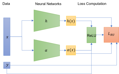
Figure 1: Model architecture for RU Regression.

Following best practices in applied machine learning, we implement our baselines and proposed method using neural networks (Goodfellow et al., 2016). From a statistical perspective, neural networks can be seen as a practical alternative to sieve methods that automate the selection of relevant basis functions (Chen and White, 1999; Farrell et al., 2021; Schmidt-Hieber, 2020). The benefits of neural networks include that they can be used as a black-box primitive for flexible function classes, they are straightforward to train using standard deep learning libraries, and they require less manual hyperparameter tuning than classical sieve-based approaches.

A neural network can be thought of as a function $f_{\theta}:\mathcal{X}\rightarrow\mathbb{R}$, where $\theta$ denotes the parameters of the network. The output space of the neural network is often the space of outcomes $\mathcal{Y}$ but can also take other values. We use Pytorch, a standard deep learning library, to instantiate, train, validate, and test the neural networks (Paszke et al., 2019). Using the Pytorch library, it is straightforward to compute the training loss, update the parameters of the network during training using a variant of stochastic gradient descent called Adam optimization (Kingma and Ba, 2014), measure the validation loss the network incurs during training, and save the network parameters that yield the lowest validation loss for later evaluation at test-time.

Our proposed method, Rockafellar-Uryasev regression, is implemented using two neural networks. One of the networks represents the decision rule $h:\mathcal{X}\rightarrow\mathcal{Y}$, while the other network represents the auxiliary function $\alpha:\mathcal{X}\rightarrow\mathbb{R}.$ A visualization for the model architecture is provided in Figure 1. Recall from Theorem 2 that RU Regression is a joint optimization over both $(h,\alpha)$. Mirroring this in our implementation, we propose to learn the parameters of the networks $h$ and $\alpha$ simultaneously. To do so, the covariates $X$ from a training sample $(X,Y)$ are passed to both networks $h$ and $\alpha$, and the outputs of both networks $h(X),\alpha(X)$ are obtained. Next, we compute $L_{\text{RU}}^{\Gamma}(h(X),\alpha(X),Y)$ by summing the three terms of the RU loss (9). Recall that the third term of the RU loss depends on $(L(h(X),Y)-\alpha(X))_{+}$. This term can be represented as $\text{ReLU}(L(h(X),Y)-\alpha(X))$, where the ReLU (rectified linear unit) function is a commonly used neural network “activation” or transform available in Pytorch. After computing the loss, we can compute the gradient of the RU loss with respect to the parameters of network $h$ and the parameters of network $\alpha$ and update the parameters of both networks using the Adam optimizer.

4.2 Simulations with Synthetic Data

We perform two simulations with synthetic data. We first consider a one-dimensional toy example because it permits visualization of the data distributions and the learned models. Next, we show that similar trends hold in a high-dimensional simulation. Implementation details for these experiments can be found in Appendix A.

4.2.1 Methods

We compare the performance of two baselines and our proposed method.

1. Standard ERM - We fit a neural network model with the squared loss function

   $$L(z,y)=(y-z)^{2}$$ (37)

   on the training data.

2. Oracle ERM - We fit a neural network model with the squared loss function (37) on data sampled from the test distribution.

3. Rockafellar-Uryasev Regression (RU Regression) - We fit two neural networks with the RU loss on the training data.

The two baselines, Standard ERM and Oracle ERM, are each implemented using a single neural network, which represents the decision rule $h:\mathcal{X}\rightarrow\mathcal{Y}.$ Both methods are trained using the squared loss function. Standard ERM and RU Regression are trained on samples from the training distribution (which may differ from the test distribution), while Oracle ERM is given access to data sampled from the test distribution at train-time. Additional implementation details are in Appendix A.

4.2.2 One-Dimensional Toy Example

Data Generation. We generate a synthetic dataset of samples of the form $(X_{i},Y_{i},U_{i}),$ where $X_{i}\in\mathbb{R}$ represents observed covariates, $Y_{i}\in\mathbb{R}$ represents the outcome, and $U_{i}\in\{0,1\}$ represents an unobserved variable that influences the outcome $Y_{i}.$ We suppose the data is distributed as follows

$$X_{i}\sim\text{Uniform}[0,10],\quad U_{i}\sim\text{Bernoulli}(p),\quad Y_{i}|X_{i}\sim N(\sqrt{X}_{i}+U_{i}(3\sqrt{X}_{i}+1),1).$$ (38)

The outcomes $Y_{i}$ can be clustered into two bands corresponding to $U_{i}=1$ and $U_{i}=0,$ respectively. In this simulation, we consider a biased training distribution where $p=0.2,$ so we are less likely to observe examples with $U_{i}=1$. Meanwhile, the possible test distributions are generated by varying $p$, e.g. $p\in\{0.1,0.2,0.5,0.7,0.9\}.$ These data distributions are visualized in Figure 2. For all methods, the train, validation, and test sets consists of 7000, 1400, and 10000 samples, respectively.

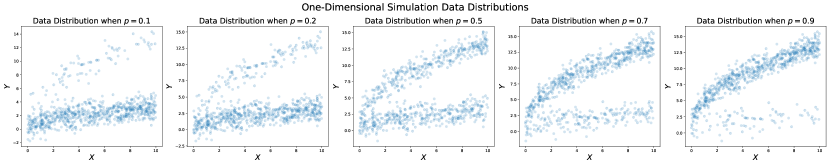
Figure 2: From left to right, we visualize the distribution over $(X_{i},Y_{i})$ as $p$ varies in $\{0.1,0.2,0.5,0.7,0.9\}.$ We note that as $p$ increases the proportion of samples where $U_{i}=1$ increases.

Results. When the test distributions have $p\in\{0.1,0.2\}$, the training distribution, which has $p=0.2$, is generated with a low amount of sampling bias. In Table 1, we observe that Standard ERM achieves low test MSE in these cases.

However, for test distributions with $p\in\{0.5,0.7,0.9\}$, the training distribution is a more biased sample of the test distribution. In these cases, we observe that Standard ERM yields high test MSE. The RU Regression methods achieve higher test MSE on the original training distribution than Standard ERM but are more robust than Standard ERM in the presence of sampling bias. Note that Oracle ERM outperforms both the Standard ERM and RU Regression methods; this is expected because the Oracle ERM model is trained on data from the same distribution as the test distribution.

In addition, we visualize the regression functions learned from each of the methods. From the left plot of Figure 3, it is clear that the regression model learned via Standard ERM incurs high error on samples with $U_{i}=1$ and low error on samples with $U_{i}=0,$ which explains why the method performs poorly on distributions with higher $p$ (higher proportion of samples with $U_{i}=1$). Furthermore, we observe that increasing $\Gamma$ yields regression functions that incur lower error on samples with $U_{i}=1$, relative to the Standard ERM model. The Oracle ERM model visualized in Figure 3 is the model that is trained on data generated when $p=0.5$. We see that this model makes similar predictions as the RU Regression models, which explains why the RU Regression models perform similarly to the Oracle ERM model on the $p=0.5$ test distribution.

Furthermore, we verify that the solution learned by the neural network is consistent with Theorem 9, which states that

$$\alpha_{\Gamma}^{*}(x)=q_{\eta(\Gamma)}^{L}(x;h_{\Gamma}^{*}(x))\quad\forall x\in\mathcal{X}.$$

For each RU Regression method, we plot the function $\hat{\alpha}_{\Gamma}(x)$ learned by the neural network. In addition, with access to the data generating process, we can explictly compute the function $q_{\eta(\Gamma)}^{L}(X;\hat{h}_{\Gamma}(X)).$ In the right plot of Figure 3, we observe that $\hat{\alpha}_{\Gamma}$ closely matches $q_{\eta(\Gamma)}^{L}(X;\hat{h}_{\Gamma}(X))$ across the possible values of $X$.

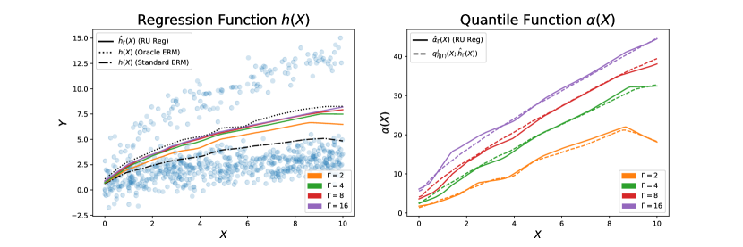
Figure 3: Left: We visualize the decision rules $\hat{h}$ that are learned in our one-dimensional toy example. Standard ERM incurs low error on samples with $U_{i}=0$ but high error on samples with $U_{i}=1$. Models learned via RU Regression incur lower error on samples with $U_{i}=1$. The Oracle ERM model visualized here is the model that is trained on the data distribution when $p=0.5$. Right: We visualize the auxiliary function $\hat{\alpha}_{\Gamma}$ that is learned in the RU Regression methods for our one-dimensional toy example. We realize that the learned $\hat{\alpha}_{\Gamma}$ closely tracks $q_{\eta(\Gamma)}^{L}(x;\hat{h}_{\Gamma}(x))$ as expected.

Method	Test MSE
	$p=0.1$	$p=0.2$	$p=0.5$	$p=0.7$	$p=0.9$
Standard ERM	6.939 $\pm$ 0.174	10.480 $\pm$ 0.126	20.866 $\pm$ 0.304	27.880 $\pm$ 0.484	34.913 $\pm$ 0.668
RU Regression	10.074 $\pm$ 0.247	11.846 $\pm$ 0.138	17.029 $\pm$ 0.236	20.522 $\pm$ 0.308	24.046 $\pm$ 0.540
($\Gamma=2$)
RU Regression	12.456 $\pm$ 0.431	13.388 $\pm$ 0.309	16.093 $\pm$ 0.179	17.898 $\pm$ 0.300	19.750 $\pm$ 0.584
($\Gamma=4$)
RU Regression	13.419 $\pm$ 0.306	14.057 $\pm$ 0.255	15.895 $\pm$ 0.133	17.119 $\pm$ 0.143	18.388 $\pm$ 0.304
($\Gamma=8$)
RU Regression	13.613 $\pm$ 0.400	14.197 $\pm$ 0.308	15.873 $\pm$ 0.140	16.983 $\pm$ 0.262	18.142 $\pm$ 0.480
($\Gamma=16$)
Oracle ERM	6.306 $\pm$ 0.187	10.480 $\pm$ 0.126	15.743 $\pm$ 0.152	13.341 $\pm$ 0.123	6.274 $\pm$ 0.176

Table 1: Results from the one-dimensional simulation experiment. We report the mean and standard deviation of the test MSE from 6 random trials, where the randomness is over the dataset generation. Standard ERM incurs high test MSE for high values of $p$. RU Regression is more robust to sampling bias than Standard ERM. RU Regression matches the performance of Oracle ERM at $p=0.5$.

4.2.3 High-Dimensional Experiment

Data Generation. We generate a synthetic dataset of samples of the form $(X_{i},Y_{i},U_{i}),$ where $X_{i}\in\mathbb{R}^{d}$ represents observed covariates, $Y_{i}\in\mathbb{R}$ represents the outcome, and $U_{i}\in\{0,1\}$ represents an unobserved variable that influences the outcome $Y_{i}.$ Since we aim to consider a high-dimensional example, we set $d=16$. We suppose the data is distributed as follows

$$X_{i}\sim\text{Uniform}[0,1]^{d},\quad U_{i}\sim\text{Bernoulli}(p),\quad Y_{i}|X_{i}\sim N(\mathbf{a}^{T}X_{i}+0.5\cdot U_{i},0.1),$$ (39)

where $\mathbf{a}\in\mathbb{R}^{d}$ is a constant vector. Similar to the one-dimensional example, the outcomes $Y_{i}$ can be clustered into two hyperplanes $Y_{i}=\mathbf{a}^{T}X_{i}+0.5$ for samples with $U_{i}=1$ and $Y=\mathbf{a}^{T}X_{i}$ for samples with $U_{i}=0.$ As in the one-dimensional example, we consider distribution shifts which result from varying $p$, the probability that $U_{i}=1$. We consider a biased training distribution where $p=0.2$, so examples with $U_{i}=1$ occur with lower frequency than examples with $U_{i}=0$. At test-time, we evaluate the learned models on data distributions where $p\in\{0.1,0.2,0.5,0.7,0.9\}.$ For all methods, the train, validation, and test sets consists of 100000, 20000, and 20000 samples, respectively.

Results. The results from the high-dimensional simulation are consistent with those from the one-dimensional simulation. From Table 2, Standard ERM achieves low test MSE when the amount of sampling bias is low, meaning that the test distribution has $p\in\{0.1,0.2\}$. However, the test MSE of Standard ERM increases when the amount of sampling bias is high, when $p\in\{0.5,0.7,0.9\}$. The RU Regression methods achieve higher test MSE on the original training distribution than Standard ERM but are more robust than Standard ERM under sampling bias. We note that RU Regression matches the performance of the Oracle ERM model when $p=0.5$.

Method	Test MSE
	$p=0.1$	$p=0.2$	$p=0.5$	$p=0.7$	$p=0.9$
Standard ERM	0.028 $\pm$ 0.000	0.043 $\pm$ 0.000	0.088 $\pm$ 0.002	0.118 $\pm$ 0.002	0.148 $\pm$ 0.003
RU Regression	0.041 $\pm$ 0.002	0.049 $\pm$ 0.001	0.071 $\pm$ 0.001	0.086 $\pm$ 0.003	0.100 $\pm$ 0.004
($\Gamma=2$)
RU Regression	0.054 $\pm$ 0.008	0.057 $\pm$ 0.006	0.067 $\pm$ 0.002	0.073 $\pm$ 0.006	0.080 $\pm$ 0.011
($\Gamma=4$)
RU Regression	0.056 $\pm$ 0.003	0.058 $\pm$ 0.002	0.066 $\pm$ 0.001	0.071 $\pm$ 0.002	0.076 $\pm$ 0.004
($\Gamma=8$)
RU Regression	0.057 $\pm$ 0.003	0.059 $\pm$ 0.002	0.066 $\pm$ 0.000	0.070 $\pm$ 0.002	0.074 $\pm$ 0.003
($\Gamma=16$)
Oracle ERM	0.025 $\pm$ 0.000	0.043 $\pm$ 0.000	0.066 $\pm$ 0.000	0.056 $\pm$ 0.000	0.025 $\pm$ 0.000

Table 2: Results from the high-dimensional $(d=16)$ simulation experiment. We report the mean and standard deviation of the test MSE from 6 random trials, where the randomness is over the dataset generation. Standard ERM incurs high test MSE for high values of $p$, where the amount of sampling bias is high. RU Regression is more robust to sampling bias than Standard ERM. RU Regression matches the performance of Oracle ERM at $p=0.5$.

4.3 MIMIC-III Data

Accurate patient length-of-stay predictions are useful for scheduling and hospital resource management (Harutyunyan et al., 2019). Many recent works study the problem of predicting patient length-of-stay from patient covariates (Daghistani et al., 2019; Morton et al., 2014; Sotoodeh and Ho, 2019). In this experiment, we evaluate our approach on electronic health record data drawn from the publicly available MIMIC-III dataset (Johnson et al., 2016a). We study the robustness of regression models when the distribution of patients observed at test time differs from the distribution of patients observed at train-time.

Data. In this experiment, the observed covariates $X_{i}$ consist of 17 different medical measurements of a patient recorded within the first 24 hours of hospital stay (see Appendix A.3 for details on the particular covariates). The outcome $Y_{i}$ is the patient length-of-stay in the ICU in days. We split the original dataset into train, validation, and test sets consisting of 7045, 4697, and 7829 samples, respectively.

To simulate a setting where the data we observed is a biased draw from our true target distribution, we imagine that datapoints from the true underlying distribution are observed with probability $\pi_{i}=1/Y_{i}$ (i.e., using notation from Definition 1, we have $\mathbb{P}\left[S_{i}\,\big{|}\,Y_{i}=y\right]=1/y$). Under this assumption, we can use the test set to get unbiased estimates for the loss of a rule learned on the training set given new draws from either the training set, or the true target distribution:

$$\begin{split}&\text{Training Environment MSE}=\sum_{i=1}^{n_{\text{test}}}L(h(X_{i}),Y_{i})\,\big{/}\,n_{\text{test}}\\ &\text{Target Environment MSE}=\sum_{i=1}^{n_{\text{test}}}\pi_{i}^{-1}L(h(X_{i}),Y_{i})\,\big{/}\,\sum_{i=1}^{n_{\text{test}}}\pi_{i}^{-1}.\end{split}$$ (40)

We note that these $\pi_{i}$ remain unobserved, and are not used for any algorithm in learning. They are simply used to define a hypothetical target environment under which we seek to perform well despite biased sampling (with unknown sampling bias).

We compare the following methods.

1. Standard ERM - We fit a neural network model with the squared loss function (Equation 37) on the training data.

2. Rockafellar-Uryasev Regression (RU Regression) - We fit two neural networks with the $L^{\Gamma}_{\text{RU}}$ loss function, where one network learns $h$ and the other network learns $\alpha$, on the training data. The model architecture is visualized in Figure 1.

Results. As seen in Table 3, RU Regression trades performance on the training distribution for robustness to sampling bias. RU Regression performs worse than standard ERM in the training environment but is more accurate than the Standard ERM in the the target environment, where patients with high length-of-stay occur with higher frequency than in the training environement. Thus, at a modest cost in shift-free accuracy, our method achieved considerable improvements in the presence of sampling bias. We emphasize that RU Regression was not given any information on how the test set might differ from the training set; we simply posited that the shift is some re-weighting of the type (8) and asked RU Regression to be robust to any such shift (up to a factor $\Gamma=3$). We report the bootstrap standard error obtained with 5000 bootstrap samples.

Method	Weighted Test MSE
	Training Environment	Target Environment
Standard ERM	3.230 $\pm$ 0.079	6.926 $\pm$ 0.265
RU Regression	3.227 $\pm$ 0.074	6.663 $\pm$ 0.253
($\Gamma=1.50$)
RU Regression	3.274 $\pm$ 0.072	6.607 $\pm$ 0.247
($\Gamma=2.00$)
RU Regression	3.349 $\pm$ 0.070	6.313 $\pm$ 0.237
($\Gamma=2.50$)
RU Regression	3.441 $\pm$ 0.068	6.060 $\pm$ 0.224
($\Gamma=3.00$)

Table 3: Results from MIMIC-III Experiment. We report the weighted test MSE and bootstrap standard error with 5000 bootstrap samples.

5 Discussion

In this paper, we considered a model for sampling bias, $\Gamma$-biased sampling, and proposed an approach to learning minimax decision rules under $\Gamma$-biased sampling. Under our model, selection bias may depend on unobservables—and the analyst may not be able to model sampling bias. As such, the optimal decision rule under the target distribution is not identified; and the best the analyst can do is to seek a decision rule with minimax guarantees under all target distributions that may have generated the observed data under $\Gamma$-biased sampling. One of our key results is that, although our learning problem may at first appear intractable, we can in fact turn it into a convex problem over an augmented function space by leveraging a result of Rockafellar and Uryasev (2000).

One question we have not focused on in this paper is how to choose $\Gamma$ in practice, i.e., how to set the maximal bias parameter in Definition 1. We emphasize that $\Gamma$ is not something that’s identified from the data; rather, it’s a parameter that the decision maker must choose when designing their learning algorithm. Setting $\Gamma=1$ corresponds to the usual empirical risk minimization algorithm, with no robustness guarantees under potential sampling bias. Using a larger value $\Gamma>1$ enables the analyst to gain robustness to sampling bias at the cost of potentially worsening performance in the training environment.

One practical way to navigate the choice of $\Gamma$ is, following Imbens (2003), to consider values of $\Gamma$ that help make decision rules robust across different available samples. For example, if one seeks to design a generally applicable risk prediction model using data only from two hospitals $A$ and $B$ whose patients come from different populations, one could examine which values of $\Gamma$ enable one to use data from hospital $A$ that work well in hospital $B$, and vice-versa. While such an exercise does not tell us which value would be best for accuracy on the (unknown) target distribution, it can at least shed light on the order of magnitude of values for $\Gamma$ that are likely to be helpful in practice.

Finally, we note that it is interesting to consider how our results relate to the broader literature on “robust” learning. There is a broad literature on methods for learning that are robust to data contamination. For example, there has been interest in models where a fraction $\varepsilon$ of the data comes from a different distribution (Chen et al., 2016; Huber, 1964), or was chosen by an adversary (Charikar et al., 2017; Diakonikolas et al., 2019; Lugosi and Mendelson, 2021). Interestingly, however, methods that seek robustness to data corruption effectively down-weight the influence of outliers, because otherwise a small fraction of corrupted examples could affect results arbitrarily much. In contrast, in our setting, we tend to give larger weight to samples with large loss—because under biased sampling a small number of samples with large loss in the training distribution could reflect a much larger fraction of the true target. In other words, approaches that seek robustness to data corruption end up to a large extent doing the opposite of what we do here in order to achieve robustness to sampling bias. This tension suggests that a learning algorithm cannot simply be “robust”. One can make choices that make an algorithm robust to some possible problems with the training distribution (e.g., sampling bias, or data corruption), but these choices will involve trade-offs that may reduce robustness across other dimensions.

Appendix A Experiment Details

A.1 One-Dimensional Toy Example

A.1.1 Models

For the Standard ERM and Oracle ERM models, we train a neural network with 2 hidden layers and 128 units per layer and ReLU activation to learn the regression function $h$. For the RU Regression model, we jointly train two neural networks to learn the regression function $h$ and the quantile function $\alpha$, respectively. A visualization of the model architecture for RU Regression is provided in Figure 1. Each of the neural networks has 2 hidden layers and 64 units per layer and ReLU activation. We note that overall the Standard ERM and Oracle ERM models have 18.8K trainable parameters, and the RU Regression model has 10.6K trainable parameters.

A.1.2 Dataset Splits

For all methods, the train, validation, and test sets consists of 7000, 1400, and 10000 samples, respectively. For Standard ERM and RU Regression, the train and validation sets are generated via the data model specified in Equation 38 with $p=0.2$. For Oracle ERM, the train and validation set is generated with the same data model with the parameter $p$ matching that of the test distribution. All methods are evaluated on the same test sets, which are generated via the data model in Equation 38 with parameter $p$ taking value in $[0.1,0.2,0.5,0.7,0.9].$ For each of 6 random seeds [0, 1, 2, 3, 4, 5], a new dataset (Standard ERM/RU Regression train and validation sets, Oracle ERM train and validation sets, and test sets) is generated.

A.1.3 Training Procedure

The models are trained for a maximum of 100 epochs with batch size equal to 1750 and we use the Adam optimizer with learning rate 1e-2. Each epoch we check the loss obtained on the validation set and select the model that minimizes the loss on the validation set.

A.2 High-Dimensional Experiment

A.2.1 Models

We use the same models as in the one-dimensional experiment. See Section A.1.1 for details.

A.2.2 Dataset Splits

For all methods, the train, validation, and test sets consists of 100000, 20000, and 20000 samples, respectively. In the data model in Equation 39, we set

$$\mathbf{a}=[ 0.098,0.430,0.206,0.090,-0.153,0.292,-0.125,0.784,$$

$$0.927,-0.233,0.583,0.0578,0.136,0.851,-0.858,-0.826]$$

in all experiments. For Standard ERM and RU Regression, the train and validation sets are generated via Equation 39 with $p=0.2$. For Oracle ERM, the train and validation set is generated with the same data model with the parameter $p$ matching that of the test distribution. All methods are evaluated on the same test sets, which are generated via the data model in Equation 39 with parameter $p$ taking value in $[0.1,0.2,0.5,0.7,0.9].$ For each of 6 random seeds [0, 1, 2, 3, 4, 5], a new dataset (Standard ERM/RU Regression train and validation sets, Oracle ERM train and validation sets, and test sets) is generated.

A.2.3 Training Procedure

The models are trained for a maximum of 50 epochs with batch size equal to 25000 and we use the Adam optimizer with learning rate 1e-2. Each step we check the loss obtained on the validation set and select the model that minimizes the loss on the validation set.

A.3 MIMIC-III Experiment

A.3.1 Dataset

Medical Information Mart for Intensive Care III (MIMIC-III) is a freely accessible medical database of critically ill patients admitted to the intensive care unit (ICU) at Beth Israel Deaconess Medical Center (BIDMC) from 2001 to 2012 [Johnson et al., 2016b, Goldberger et al., 2000]. During that time, BIDMC switched clinical information systems from Carevue (2001-2008) to Metavision (2008-2012). To ensure data consistency, only data archived via the Metavision system was used in the dataset.

A.3.2 Feature Selection and Data Preprocessing

We select the same patient features and imputed values as in Harutyunyan et al. [2019]. A total of 17 variables were extracted from the chartevents table to include in the dataset - capillary refill rate, blood pressure (systolic, diastolic, and mean), fraction of inspired oxygen, Glasgow Coma Score (eye opening response, motor response, verbal response, and total score), serum glucose, heart rate, respiratory rate, oxygen saturation, respiratory rate, temperature, weight, and arterial pH. For each unique ICU stay, values were extracted for the first 24 hours upon admission to the ICU and averaged. Normal values were imputed for missing variables as shown in Table 4.

Variable	MIMIC-III item ids from chartevents table	Imputed value
Capillary refill rate	(223951, 224308)	0
Diastolic blood pressure	(220051, 227242, 224643, 220180, 225310)	59.0
Systolic blood pressure	(220050, 224167, 227243, 220179, 225309)	118.0
Mean blood pressure	(220052, 220181, 225312)	77.0
Fraction inspired oxygen	(223835)	0.21
GCS eye opening	(220739)	4
GCS motor response	(223901)	6
GCS verbal response	(223900)	5
GCS total	(220739 + 223901 + 223900)	15
Glucose	(228388, 225664, 220621, 226537)	128.0
Heart Rate	(220045)	86
Height	(226707, 226730)	170.0
Oxygen saturation	(220227, 220277, 228232)	98.0
Respiratory rate	(220210, 224688, 224689, 224690)	19
Temperature	(223761, 223762)	97.88
Weight	(224639, 226512, 226531)	178.6
pH	(223830)	7.4

Table 4: Variables included in dataset

Following the cohort selection procedure in Wang et al. [2020], we further restrict to patients with covariates within physiologically valid range of measurements and length-of-stay less than or equal to 10 days.

A.3.3 Training Details

Models. For the Standard ERM model, we train a neural network with 2 hidden layers and 128 units per layer and ReLU activation to learn the regression function $h$. For the RU Regression model, we jointly train two neural networks to learn the regression function $h$ and the quantile function $\alpha$, respectively. Each of the neural networks has 2 hidden layers and 64 units per layer and ReLU activation. A visualization of the model architecture for RU Regression is provided in Figure 1. We note that overall the Standard ERM model has 18.8K trainable parameters, and the RU Regression model has 10.6K trainable parameters.

Dataset Splits. For all methods, the train, validation, and test sets consists of 7045, 4697, and 7829 samples, respectively.

Appendix B Standard Results

Definition 4.

A function $h$ on $\mathcal{X}$ is said to satisfy a Holder condition with exponent $\beta$ if there is a positive number $\gamma$ such that $|h(x)-h(x_{0})|\leq\gamma|x-x_{0}|^{\beta}$ for $x_{0},x\in\mathcal{X}.$

Lemma 16.

If there is a function $Q_{0}(\theta)$ such that (i) $Q_{0}(\theta)$ is uniquely maximized at $\theta_{0}$; (ii) $\theta_{0}$ is an element of the interior of a convex set $\Theta$ and $\hat{Q}_{n}(\theta)$ is concave; and (iii) $\hat{Q}_{n}(\theta)\rightarrow Q_{0}(\theta)$for all $\theta\in\Theta$, then $\hat{\theta}_{n}$ exists with probability approaching one and $\hat{\theta}_{n}\xrightarrow{p}\theta_{0}$ (Theorem 2.7, Newey and McFadden [1994]).

Lemma 17.

If a functional $J:V\rightarrow\mathbb{R}$ is Gâteaux differentiable $J^{\prime}$ at $u_{0}\in V$ and has a relative extremum at $u_{0}$, then $J^{\prime}(u_{0};v)=0$ for all $v\in V.$

Lemma 18.

If $\{e_{i}\}$ is an orthonormal basis (a maximal orthonormal sequence) in a Hilbert space $H$ then for any element $u\in H$ the ‘Fourier-Bessel series‘ converges to $u$:

$$u=\sum_{i=1}^{\infty}\langle u,e_{i}\rangle e_{i}.$$

Lemma 19.

Let $X$ be a Hilbert space, and suppose $f:X\rightarrow[-\infty,\infty]$ is lower semicontinuous and convex. If $C$ is a closed, bounded, and convex subset of $X$, then $f$ achieves its minimum on $C$; i.e., there is some $x_{0}\in C$ with $f(x_{0})=\inf_{x\in C}f(x).$

Lemma 20.

Let $A$ be a $2\times 2$ symmetric matrix with $\operatorname{tr}(A)>0$ and $\det(A)\geq 0$. Then

$$\lambda_{\min}(A)\geq\frac{\det A}{\operatorname{tr}A},\quad\lambda_{\max}(A)\leq\operatorname{tr}A.$$

Proof in Appendix D.3.

Lemma 21.

Let $H(h,\alpha)=G(h)+F(h,\alpha),$ where $G$ is strongly convex and Gâteaux differentiable in $h$ and $F$ is jointly convex in $(h,\alpha)$, strictly convex in $\alpha$, and Gâteaux differentiable in $(h,\alpha)$. Then $H$ is strictly convex in $(h,\alpha).$ Proof in Appendix D.4.

Appendix C Proofs of Main Results

C.1 Notation

We introduce notation that is used in the proofs and technical lemmas.

$$L_{\text{RU},1}^{\Gamma}(z,y) :=\Gamma^{-1}L(z,y)$$ (41)

$$L_{\text{RU},2}^{\Gamma}(a) :=(1-\Gamma^{-1})a$$ (42)

$$L_{\text{RU},3}^{\Gamma}(z,y,a) :=(\Gamma-\Gamma^{-1})\cdot(L(z,y)-a)_{+}.$$ (43)

Define

$$R_{f,c} :=\{x\in\mathcal{X}\mid f(x)<c\}$$ (44)

$$S_{f,c} :=\{x\in\mathcal{X}\mid f(x)>c\}.$$ (45)

When we consider loss functions $L$ that satisfy Assumption 2, we define

$$\ell_{1}(y) :=\left\{\begin{array}[]{cc}\ell(y)&y>0\\ 0&y\leq 0\end{array}\right.,\quad\ell_{2}(y):=\left\{\begin{array}[]{cc}0&y>0\\ \ell(y)&y\leq 0\end{array}\right.,$$ (50)

$$T_{1,x}(c) :=\mathbb{E}_{P_{Y|X=x}}\left[\ell(Y-c)\mid X=x\right],$$ (51)

$$T_{3,x}(c,d) :=\begin{cases}\mathbb{E}_{P_{Y|X=x}}\left[(\ell(Y-c)-d)\mathbb{I}(\ell(Y-c)>d)\mid X=x\right]&d>0\\ \mathbb{E}_{P_{Y|X=x}}\left[\ell(Y-c)-d\mid X=x\right]&d\leq 0\\ \end{cases}.$$ (52)

C.2 Technical Lemmas

We prove lemmas about the transforms $T_{1,x}(c),T_{3,x}(c,d)$. These enable us to establish more general properties of the RU loss.

Lemma 22.

Under Assumption 2, $T_{1,x}(c)$ is twice-differentiable in $c$ and

$$\mathbb{E}_{P}\left[L_{\text{RU},1}^{\Gamma}(h(X),Y)\right]=\Gamma^{-1}\mathbb{E}_{P_{X}}\left[T_{1,X}(h(X))\right].$$

Proof in Appendix D.5.

Lemma 23.

Under Assumption 2, 3, $T_{3,x}(c,d)$ is differentiable in $c,d$. In particular,

$$T_{3,x}^{d}(c,d)=\begin{cases}-\Pr(\ell(Y-c)>d\mid X=x)&d>0\\ -1&d\leq 0\end{cases}.$$

Equivalently,

$$T_{3,x}^{d}(c,d)=\begin{cases}-1+P_{Y|X=x}(c+\ell_{1}^{-1}(d))-P_{Y|X=x}(c+\ell_{2}^{-1}(d))&d>0\\ -1&d\leq 0\end{cases}.$$

In addition, $T_{3,x}(c,d)$ is twice-differentiable in $c,d$ when $d>0.$ The second derivatives are

$$T_{3,x}^{cc}(c,d) =\sum_{i\in\{1,2\}}|\ell^{\prime}(\ell_{i}^{-1}(d))|\cdot p_{Y|X=x}(c+\ell_{i}^{-1}(d))+\mathbb{E}_{P_{Y|X}}\left[\ell^{\prime\prime}(Y-c)\mathbb{I}(\ell(Y-c)>d)\right],$$

$$T_{3,x}^{dd}(c,d) =\sum_{i\in\{1,2\}}\frac{p_{Y|X=x}(c+\ell_{i}^{-1}(d))}{|\ell^{\prime}(\ell^{-1}_{i}(d))|},$$

$$T_{3,x}^{cd}(c,d) =p_{Y|X=x}(c+\ell_{1}^{-1}(d))-p_{Y|X=x}(c+\ell_{2}^{-1}(d)),$$

where $\ell_{1}^{-1}$ is the inverse of $\ell(z)$ when $z>0$ and $\ell_{2}^{-1}$ is the inverse of $\ell(z)$ when $z<0.$

Also,

$$\mathbb{E}_{P}\left[L_{\text{RU},3}^{\Gamma}(h(X),\alpha(X),Y)\right]=(\Gamma-\Gamma^{-1})\mathbb{E}_{P_{X}}\left[T_{3,X}(h(X),\alpha(X))\right].$$

Proof in Appendix D.6.

Lemma 24.

Under Assumption 2, 3, there are symmetric matrices $A_{x}(c,d),B_{x}(c,d)$ such that

$$A_{x}(c,d)\preceq\nabla^{2}T_{3,x}(c,d)\preceq B_{x}(c,d)$$

when $d>0$. The entries of $A_{x}(c,d)$ are given by

$$A_{x,11}(c,d) =\sum_{i\in\{1,2\}}|\ell^{\prime}(\ell_{i}^{-1}(d))|\cdot p_{Y|X=x}(c+\ell_{i}^{-1}(d))+C_{L,l}\cdot\Pr(\ell(Y-c)>d\mid X=x)$$

$$A_{x,22}(c,d) =\sum_{i\in\{1,2,\}}\frac{p_{Y|X=x}(c+\ell_{i}^{-1}(d))}{|\ell^{\prime}(\ell^{-1}_{i}(d))|},$$

$$A_{x,12}(c,d) =p_{Y|X=x}(c+\ell_{1}^{-1}(d))-p_{Y|X=x}(c+\ell_{2}^{-1}(d)).$$

The entries of $B_{x}(c,d)$ are given by

$$B_{x,11}(c,d) =\sum_{i\in\{1,2\}}|\ell^{\prime}(\ell_{i}^{-1}(d))|\cdot p_{Y|X=x}(c+\ell_{i}^{-1}(d))+\mathbb{E}_{P_{Y|X=x}}\left[\ell^{\prime\prime}(Y-c)\mid X=x\right],$$

$$B_{x,22}(c,d) =\sum_{i\in\{1,2\}}\frac{p_{Y|X=x}(c+\ell_{i}^{-1}(d))}{|\ell^{\prime}(\ell^{-1}_{i}(d))|},$$

$$B_{x,12}(c,d) =p_{Y|X=x}(c+\ell_{1}^{-1}(d))-p_{Y|X=x}(c+\ell_{2}^{-1}(d)).$$

Proof in Appendix D.7.

We give a few additional lemmas related to the RU loss. These lemmas are used in proofs of many of the results from Section 3.1.

Lemma 25.

Under Assumption 1, 2 3, $\mathbb{E}_{P}\left[L_{\text{RU}}^{\Gamma}(h(X),\alpha(X),Y)\right]$ is Gâteaux differentiable in $(h,\alpha)$ on $L^{2}(P_{X},\mathcal{X})\times L^{2}(P_{X},\mathcal{X})$ and twice-Gâteaux differentiable in $(h,\alpha)$ on $\mathcal{C}$, where

$$\mathcal{C}=\{(h,\alpha)\in\Theta\mid\alpha(x)>0\quad\forall x\in\mathcal{X}\}.$$

Proof in Appendix D.8.

Lemma 26.

Under Assumption 2, $\mathbb{E}_{P}\left[L_{\text{RU},1}^{\Gamma}(h(X),Y)\right]$ is strongly convex in $h$. Proof in Appendix D.9.

Lemma 27.

Under Assumptions 1, 2, 3, $\mathbb{E}_{P}\left[L_{\text{RU},3}^{\Gamma}(h(X),\alpha(X),Y)\right]$ is strictly convex in $\alpha$ on $\mathcal{A}$.

Proof in Appendix D.10.

C.3 Proof of Lemma 1

First, suppose that $Q$ generates $P$ via $\Gamma$-biased sampling. We show that (8) holds and that $\sup_{x\in\mathcal{X}}\frac{dP_{X}(x)}{dQ_{X}(x)}<C$ for some $C<\infty.$

$$\frac{dQ_{Y\mid X=x}(y)}{dP_{Y\mid X=x}(y)} =\frac{d\tilde{Q}_{Y\mid X}(y)}{d\tilde{Q}_{Y\mid X,S=1}(y)}$$ (53)

$$=\frac{d\tilde{Q}_{X,Y}(x,y)}{d\tilde{Q}_{X}(x)}\cdot\frac{d\tilde{Q}_{X\mid S=1}(x)}{d\tilde{Q}_{X,Y\mid S=1}(x,y)}$$ (54)

$$=\frac{d\tilde{Q}_{X,Y}(x,y)}{d\tilde{Q}_{X,Y\mid S=1}(x,y)}\cdot\frac{d\tilde{Q}_{X\mid S=1}(x)}{d\tilde{Q}_{X}(x)}$$ (55)

$$=\frac{d\tilde{Q}_{X,Y}(x,y)}{d\tilde{Q}_{X,Y\mid S=1}(x,y)}\cdot\frac{d\tilde{Q}_{X\mid S=1}(x)}{d\tilde{Q}_{X}(x)}\cdot\frac{\mathbb{P}_{\tilde{Q}}\left[S=1\right]}{\mathbb{P}_{\tilde{Q}}\left[S=1\right]}$$ (56)

$$=\frac{\mathbb{P}_{\tilde{Q}}\left[S=1\mid X=x\right]}{\mathbb{P}_{\tilde{Q}}\left[S=1\mid X=x,Y=y\right]}$$ (57)

$$\in[\Gamma^{-1},\Gamma].$$ (58)

(57) follows from Bayes’ Rule. (58) follows from (3). So, (8) holds.

We also show that the covariate density ratio between $P$ and $Q$ is bounded. We note that

$$dP_{X}(x) =dQ_{X}(x)\cdot\frac{\mathbb{P}_{\tilde{Q}}\left[S=1\mid X=x\right]}{\mathbb{P}_{\tilde{Q}}\left[S=1\right]}$$

$$\leq\frac{1}{\mathbb{P}_{\tilde{Q}}\left[S=1\right]}.$$

Thus, we have that $\sup_{x\in\mathcal{X}}\frac{dP_{X}(x)}{dQ_{X}(x)}$ is upper bounded by a constant.

Second, we show the converse. Let $Q$ be a distribution over $(X,Y)$ that satisfies (8). We define $\tilde{Q}$ to be a distribution over $(X,Y,S)$, where $X\in\mathcal{X},Y\in\mathcal{Y},S\in\{0,1\}.$We set $\tilde{Q}_{X,Y}=Q$ and define that

$$\mathbb{P}_{\tilde{Q}}\left[S=1\mid X=x,Y=y\right]=\frac{1}{N}\frac{dP(x,y)}{dQ(x,y)},$$ (59)

where $N\leq 1/C\Gamma$. Note that $\mathbb{P}_{\tilde{Q}}\left[S=1\mid X=x,Y=y\right]\in[0,1]$ because (8) holds and $\sup_{x\in\mathcal{X}}\frac{dP_{X}(x)}{dQ_{X}(x)}<C$.

To show that converse holds, we must verify (3) holds for $\tilde{Q}$ and that $\tilde{Q}_{X,Y\mid S=1}=P.$ First, we verify (3). We compute $\mathbb{P}_{\tilde{Q}}\left[S=1\mid X=x\right].$

$$\mathbb{P}_{\tilde{Q}}\left[S=1\mid X=x\right]=\mathbb{E}_{\tilde{Q}}\left[\frac{1}{N}\cdot\frac{dP(X,Y)}{dQ(X,Y)}\mid X=x\right]=\frac{1}{N}\cdot\frac{dP_{X}(x)}{dQ_{X}(x)}.$$ (60)

Note that

$$\mathbb{P}_{\tilde{Q}}\left[S=1\mid X=x,Y=y\right]=\frac{1}{N}\cdot\frac{dP(x,y)}{dQ(x,y)}=\mathbb{P}_{\tilde{Q}}\left[S=1\mid X=x\right]\cdot\frac{dP_{Y|X=x}(y)}{dQ_{Y|X=x}(y)}.$$

From (8), we have that

$$\frac{dP_{Y|X=x}(y)}{dQ_{Y|X=x}(y)}\in[\Gamma^{-1},\Gamma].$$

So, we have that (3) holds for $\tilde{Q}$.

Now, we can verify that $\tilde{Q}_{X,Y\mid S=1}=P$. We aim to verify that

$$d\tilde{Q}_{X,Y\mid S=1}(x,y)=dP(x,y).$$ (61)

We have that

$$d\tilde{Q}_{X,Y,S=1}(x,y) =\mathbb{P}_{\tilde{Q}}\left[S=1,X=x,Y=y\right]$$

$$=\mathbb{P}_{\tilde{Q}}\left[S=1\mid X=x,Y=y\right]\cdot\mathbb{P}_{\tilde{Q}}\left[X=x,Y=y\right]$$

$$=\frac{1}{N}\cdot\frac{dP_{X,Y}(x,y)}{dQ_{X,Y}(x,y)}\cdot dQ_{X,Y}(x,y)$$

$$=\frac{1}{N}\cdot dP(x,y).$$

In addition, from (60), we have that

$$\mathbb{P}_{\tilde{Q}}\left[S=1\right] =\mathbb{E}_{\tilde{Q}_{X}}\left[\mathbb{P}_{\tilde{Q}}\left[S=1\mid X=x\right]\right]$$

$$=\mathbb{E}_{\tilde{Q}_{X}}\left[\frac{1}{N}\cdot\frac{dP_{X}(X)}{dQ_{X}(X)}\right]$$

$$=\frac{1}{N}.$$

Thus, we have that

$$d\tilde{Q}_{X,Y\mid S=1}(x,y)=\frac{d\tilde{Q}_{X,Y,S=1}(x,y)}{\mathbb{P}_{\tilde{Q}}\left[S=1\right]}=dP_{X,Y}(x,y).$$

Therefore, we have that $Q$ can generate $P$ under $\Gamma$-biased sampling.

C.4 Proof of Lemma 5

Suppose for the sake of contradiction $(h,\alpha)$ is a minimizer of the population RU risk and $(h,\alpha)\notin\Theta.$ There are three cases

1. $(h,\alpha)\in\mathcal{H}^{c}\times\mathcal{A},$

2. $(h,\alpha)\in\mathcal{H}\times\mathcal{A}^{c},$

3. $(h,\alpha)\in\mathcal{H}^{c}\times\mathcal{A}^{c}.$

First, we focus on the case where $(h,\alpha)\in\mathcal{H}^{c}\times\mathcal{A}.$ We consider $\bar{h},$

$$\bar{h}(x)=\begin{cases}h(x)&h(x)\in[-2B,2B]\\ 2B&h(x)>2B\\ -2B&h(x)<-2B\end{cases}.$$

We note that $(\bar{h},\alpha)\in\Theta$. We define $R_{h,-2B}$ and $S_{h,2B}$ following (44) and (45).

$$\mathbb{E}_{P}\left[L_{\text{RU}}^{\Gamma}(h(X),\alpha(X),Y)\right]-\mathbb{E}_{P}\left[L_{\text{RU}}^{\Gamma}(\bar{h}(X),\alpha(X),Y)\right]$$

$$=\mathbb{E}_{P}\left[(L_{\text{RU}}^{\Gamma}(h(X),\alpha(X),Y)-L_{\text{RU}}^{\Gamma}(\bar{h}(X),\alpha(X),Y)\mathbb{I}(R_{h,-2B})\right]$$

$$\indent+\mathbb{E}_{P}\left[(L_{\text{RU}}^{\Gamma}(h(X),\alpha(X),Y)-L_{\text{RU}}^{\Gamma}(\bar{h}(X),\alpha(X),Y)\mathbb{I}(S_{h,2B})\right]$$

because they only differ on $R_{h,-2B}$ and $S_{h,2B}.$ Analyzing the second term on the right side above, we see that

$$\mathbb{E}_{P}\left[(L_{\text{RU}}^{\Gamma}(h(X),\alpha(X),Y)-L_{\text{RU}}^{\Gamma}(\bar{h}(X),\alpha(X),Y))\cdot\mathbb{I}(S_{h,2B})\right]$$

$$=\mathbb{E}_{P_{X}}\left[\Big{(}\Gamma^{-1}T_{1,X}(h(X),\alpha(X)))+(\Gamma-\Gamma^{-1})\cdot T_{3,X}(h(X),\alpha(X))\Big{)}\mathbb{I}(S_{h,2B})\right],$$

where $T_{1,X},T_{3,X}$ are defined in Lemma 22 and Lemma 23, respectively. For $x\in S_{h,2B},$

$$\Gamma^{-1}T_{1,x}(h(x),\alpha(x))+(\Gamma-\Gamma^{-1})\cdot T_{3,x}(h(x),\alpha(x))-\Gamma^{-1}T_{1,x}(\bar{h}(x),\alpha(x))-(\Gamma-\Gamma^{-1})\cdot T_{3,x}(\bar{h}(x),\alpha(x))$$

$$=(h(x)-\bar{h}(x))\cdot\Big{(}\Gamma^{-1}T_{1,x}^{c}(\tilde{h}(x),\alpha(x))+(\Gamma-\Gamma^{-1})\cdot T_{3,X}^{c}(\tilde{h}(x),\alpha(x))\Big{)}\quad\tilde{h}(x)\in[\bar{h}(x),h(x)]$$ (62a)

$$=(h(x)-\bar{h}(x))\cdot\mathbb{E}_{P_{Y|X=x}}\left[\Gamma^{-1}\cdot(-\ell^{\prime}(Y-\tilde{h}(x)))+(\Gamma-\Gamma^{-1})\cdot(-\ell^{\prime}(Y-\tilde{h}(x)))\cdot\mathbb{I}(\ell(Y-\tilde{h}(x))>\alpha(x))\right]$$ (62b)

$$\geq(h(x)-\bar{h}(x))\cdot\mathbb{E}_{P_{Y|X=x}}\left[\Gamma^{-1}\cdot(-\ell^{\prime}(Y-\tilde{h}(x)))\right]$$ (62c)

$$>0.$$ (62d)

(62a) follows from the Mean Value Theorem, the differentiability of $T_{1,x}$ (Lemma 22), and the differentiability of $T_{3,x}$ (Lemma 23). (62b) follows from Lemma 22 and Lemma 23. The inequality in (62c) comes from the observation that for $x\in S_{h,2B}$, we have that $Y-\tilde{h}(x)\leq-B$ because $Y\in[-B,B]$ and $\tilde{h}(x)\in[2B,h(x)].$ So, $-\ell^{\prime}(Y-\tilde{h}(x))>0.$ Meanwhile, $h(x)-\bar{h}(x)>0$. So, the product of $-\ell^{\prime}(Y-\tilde{h}(x))\cdot(h(x)-\bar{h}(x))>0.$ Since $\Pr(\ell(Y-\tilde{h}(x))>\alpha(x)|X=x)\geq 0,$ (62c) holds. For the same reason, (62d) holds as well. Thus, if $S_{h,2B}$ has positive measure, then

$$\mathbb{E}_{P}\left[(L_{\text{RU}}^{\Gamma}(h(X),\alpha(X),Y)-L_{\text{RU}}^{\Gamma}(\bar{h}(X),\alpha(X),Y))\mathbb{I}(X\in S_{h,2B})\right]>0.$$

An analogous argument can be used to show that for $R_{h,-2B}$ with positive measure,

$$\mathbb{E}_{P}\left[(L_{\text{RU}}^{\Gamma}(h(X),\alpha(X),Y)-L_{\text{RU}}^{\Gamma}(\bar{h}(X),\alpha(X),Y))\mathbb{I}(X\in R_{h,-2B})\right]>0.$$

Thus, as long as $R_{h,-2B}\cup S_{h,2B}$ has positive measure, which must be the case under our assumption that the minimizer $(h,\alpha)\in\mathcal{H}^{c}\times\mathcal{A},$ then there is $(\bar{h},\alpha)\in\Theta$ that achieves lower population RU risk. This is a contradiction, so the minimizer cannot be in $\mathcal{H}^{c}\times\mathcal{A}.$

Now, we consider the next case that the minimizer $(h,\alpha)\in\mathcal{H}\times\mathcal{A}^{c}.$ Consider $\bar{\alpha}\in\mathcal{A}$,

$$\bar{\alpha}(x)=\begin{cases}0&\alpha(x)<0\\ \alpha(x)&0\leq\alpha(x)\leq M_{u}\\ M_{u}&\alpha(x)>M_{u}\end{cases}$$

Note that $(h,\bar{\alpha})\in\Theta$. We define $R_{\alpha,0}$ and $S_{\alpha,M_{u}}$ according to (44) and (45), respectively. We have that

$$\mathbb{E}_{P}\left[L_{\text{RU}}^{\Gamma}(h(X),\alpha(X),Y)\right]-\mathbb{E}_{P}\left[L_{\text{RU}}^{\Gamma}(h(X),\bar{\alpha}(X),Y)\right]$$

$$=\mathbb{E}_{P}\left[(L_{\text{RU}}^{\Gamma}(h(X),\alpha(X),Y)-L_{\text{RU}}^{\Gamma}(h(X),\bar{\alpha}(X),Y))\mathbb{I}(R_{\alpha,0})\right]$$

$$\indent+\mathbb{E}_{P}\left[(L_{\text{RU}}^{\Gamma}(h(X),\alpha(X),Y)-L_{\text{RU}}^{\Gamma}(h(X),\bar{\alpha}(X),Y))\mathbb{I}(S_{\alpha,M_{u}})\right].$$

because they only differ on $R_{\alpha,0}$ and $S_{\alpha,M_{u}}$. We find that

$$\mathbb{E}_{P}\left[(L_{\text{RU}}^{\Gamma}(h(X),\alpha(X),Y)-L_{\text{RU}}^{\Gamma}(h(X),\bar{\alpha}(X),Y))\cdot\mathbb{I}(R_{\alpha,0})\right]$$

$$=(1-\Gamma^{-1})\mathbb{E}_{P}\left[(\alpha(X)-\bar{\alpha}(X))\mathbb{I}(R_{\alpha,0})\right]+(\Gamma-\Gamma^{-1})\mathbb{E}_{P}\left[(L(h(X),Y)-\alpha(X))_{+}\cdot\mathbb{I}(R_{\alpha,0})\right]$$

$$\indent-(\Gamma-\Gamma^{-1})\mathbb{E}_{P}\left[(L(h(X),Y)-\bar{\alpha}(X))_{+}\cdot\mathbb{I}(R_{\alpha,0})\right]$$

$$=(1-\Gamma^{-1})\mathbb{E}_{X}\left[\alpha(X)\mathbb{I}(R_{\alpha,0})\right]+(\Gamma-\Gamma^{-1})\mathbb{E}_{P}\left[(L(h(X),Y)-\alpha(X))\mathbb{I}(R_{\alpha,0})\right]$$

$$\indent-(\Gamma-\Gamma^{-1})\mathbb{E}_{P}\left[L(h(X),Y)\mathbb{I}(R_{\alpha,0})\right]$$

$$=(1-\Gamma)\mathbb{E}_{P}\left[\alpha(X)\cdot\mathbb{I}(R_{\alpha,0})\right].$$

If $R_{\alpha,0}$ has positive measure, then

$$\mathbb{E}_{P}\left[(L_{\text{RU}}^{\Gamma}(h(X),\alpha(X),Y)-L_{\text{RU}}^{\Gamma}(h(X),\bar{\alpha}(X),Y))\cdot\mathbb{I}(R_{\alpha,0})\right]>0$$

because on $R_{\alpha,0}$, we have that $\alpha(X)<0$ and also $(1-\Gamma)<0$. In addition,

$$\mathbb{E}_{P}\left[(L_{\text{RU}}^{\Gamma}(h(X),\alpha(X),Y)-L_{\text{RU}}^{\Gamma}(h(X),\bar{\alpha}(X),Y))\cdot\mathbb{I}(S_{\alpha,M_{u}})\right]$$

$$=\mathbb{E}_{P_{X}}\left[\mathbb{E}_{P_{Y|X}}\left[L_{\text{RU},2}^{\Gamma}(\alpha(X))-L_{\text{RU},2}^{\Gamma}(\bar{\alpha}(X))+L_{\text{RU},3}^{\Gamma}(h(X),\alpha(X),Y)-L_{\text{RU},3}^{\Gamma}(h(X),\bar{\alpha}(X),Y)\mid X\right]\mathbb{I}(S_{\alpha,M_{u}})\right].$$

For $x\in S_{\alpha,M_{u}}$, we compute

$$\mathbb{E}_{P_{Y|X}}\left[L_{\text{RU},2}^{\Gamma}(\alpha(X))-L_{\text{RU},2}^{\Gamma}(\bar{\alpha}(X))+L_{\text{RU},3}^{\Gamma}(h(X),\alpha(X),Y)-L_{\text{RU},3}^{\Gamma}(h(X),\bar{\alpha}(X),Y)\mid X=x\right]$$ (63a)

$$=\mathbb{E}_{P_{Y|X=x}}\left[(1-\Gamma^{-1})(\alpha(X)-\bar{\alpha}(X))\mid X=x\right]$$ (63b)

$$\indent+\mathbb{E}_{P_{Y|X=x}}\left[(\Gamma-\Gamma^{-1})\Big{(}T_{3,X}(h(X),\alpha(X))-T_{3,X}(h(X),\bar{\alpha}(X))\Big{)}\mid X=x\right]$$ (63c)

$$=(1-\Gamma^{-1})(\alpha(x)-\bar{\alpha}(x))+(\Gamma-\Gamma^{-1})\Big{(}T_{3,x}(h(x),\alpha(x))-T_{3,x}(h(x),\bar{\alpha}(x))\Big{)}$$ (63d)

$$=(1-\Gamma^{-1})(\alpha(x)-\bar{\alpha}(x))+(\Gamma-\Gamma^{-1})\cdot(\alpha(x)-\bar{\alpha}(x))\cdot T_{3,x}^{d}(h(x),\tilde{\alpha}(x))\quad\tilde{\alpha}(x)\in[\bar{\alpha}(x),\alpha(x)]$$ (63e)

$$=(1-\Gamma^{-1})(\alpha(x)-\bar{\alpha}(x))+(\Gamma-\Gamma^{-1})\cdot(\alpha(x)-\bar{\alpha}(x))\cdot(-1+F_{x;h(x)}(\tilde{\alpha}(x)))$$ (63f)

$$>(1-\Gamma^{-1})(\alpha(x)-\bar{\alpha}(x))+(\Gamma-\Gamma^{-1})\cdot(\alpha(x)-\bar{\alpha}(x))\cdot(-1+\eta(\Gamma))$$ (63g)

$$=0.$$ (63h)

In the above derivation, we have that (63d) follows from Lemma 23 and Assumption 2. Next, we apply the Mean Value Theorem to $T_{3,x}(c,d)$ to arrive at (63e). After that, we use the definition of $T^{d}_{3,x}(c,d)$ for $d>0$ from Lemma 23, where $\tilde{\alpha}(x)>0$. Finally, we recall that $F_{x;h(x)}$ is the distribution over $L(h(x),Y)=\ell(Y-h(x))$ when $Y$ is distributed according to $P_{Y|X=x}.$ We can show (63g) as follows. Since $\tilde{\alpha}(x)\in[\bar{\alpha}(x),\alpha(x)]$ and $x\in S_{\alpha,M_{u}},$ we have that

$$F_{x;h(x)}(\tilde{\alpha}(x))\geq F_{x;h(x)}(\bar{\alpha}(x))=F_{x;h(x)}(M_{u}),$$

and we have that

$$q^{L}_{\eta(\Gamma)}(x;h(x))=F_{x;h(x)}^{-1}(\eta(\Gamma))<M_{u}$$

by the definition of $M_{u}$ (25). So, we see that $\eta(\Gamma)<F_{x;h(x)}(M_{u})$. In addition, we note that $\alpha(x)-\bar{\alpha}(x)>0$ for $x\in S_{\alpha,M_{u}}$ and $\Gamma-\Gamma^{-1}>0$. We conclude that if $S_{\alpha,M_{u}}$ has positive measure, then

$$\mathbb{E}_{P}\left[(L_{\text{RU}}^{\Gamma}(h(X),\alpha(X),Y)-L_{\text{RU}}^{\Gamma}(h(X),\bar{\alpha}(X),Y))\cdot\mathbb{I}(S_{\alpha,M_{u}})\right]>0.$$

Thus, as long as $R_{\alpha,0}\cup S_{\alpha,M_{u}}$ has positive measure, which must be the case because we assumed that $(h,\alpha)\in\mathcal{H}\times\mathcal{A}^{c}$, there is $(h,\bar{\alpha})\in\Theta$ that achieves lower population RU risk than the minimizer $(h,\alpha)$. This is a contradiction, so any minimizer cannot be in $\mathcal{H}\times\mathcal{A}^{c}.$

Combining the two previous arguments, we can show that any minimizer also cannot be in $\mathcal{H}^{c}\times\mathcal{A}^{c}.$ Thus, any minimizer of the population RU risk must lie in $\Theta$.

C.5 Proof of Lemma 6

The main goal of this proof is to apply Lemma 19 to the function $\mathbb{E}_{P}\left[L^{\Gamma}_{\text{RU}}(h(X),\alpha(X),Y)\right]$ and set $\Theta$. Clearly, the population RU risk is continuous. We have the RU loss is convex from the first part of Theorem 2, so the population RU risk is also convex in $(h,\alpha).$ In addition, $\Theta\subset L^{2}(P_{X},\mathcal{X})\times L^{2}(P_{X},\mathcal{X})$, which is a Hilbert space. In addition, since $L^{\infty}$ balls are closed in $L^{2}(P_{X},\mathcal{X}),$ and $\Theta$ consists of a product of $L^{\infty}$ balls (one of which is not centered at 0), so $\Theta$ is closed in $L^{2}(P_{X},\mathcal{X}).$ Also, $\Theta$ is convex and bounded. Thus Lemma 19 holds, so $\mathbb{E}_{P}\left[L^{\Gamma}_{\text{RU}}(h(X),\alpha(X),Y)\right]$ must achieve a minimum on $\Theta$.

C.6 Proof of Lemma 7

Let

$$F(h,\alpha) =\mathbb{E}_{P}\left[L_{\text{RU},3}^{\Gamma}(h(X),\alpha(X),Y)\right]$$

$$G(h) =\mathbb{E}_{P}\left[L_{\text{RU},1}^{\Gamma}(h(X),Y)\right]$$

$$H(h,\alpha) =\mathbb{E}_{P}\left[L_{\text{RU},1}^{\Gamma}(h(X),Y)\right]+\mathbb{E}_{P}\left[L_{\text{RU},3}^{\Gamma}(h(X),\alpha(X),Y)\right].$$

Note that

$$\mathbb{E}_{P}\left[L_{\text{RU}}^{\Gamma}(h(X),\alpha(X),Y)\right]=H(h,\alpha)+\mathbb{E}_{P}\left[L_{\text{RU},2}^{\Gamma}(\alpha(X))\right].$$ (64)

Since the population RU risk is the sum of $H$ and a function that is convex in $(h,\alpha)$, then it suffices to show that $H$ is strictly convex. The main goal of this proof is to show that the conditions of Lemma 21 hold so that we can conclude that $H$, as defined above, is strictly convex in $(h,\alpha).$

First, we note that $F,G,H$ are all Gâteaux differentiable by Lemma 25.

Second, we show that $G$ satisfies the conditions of Lemma 21. By Lemma 26, $G$ is strongly convex with constant $\Gamma^{-1}C_{L,l}.$

Third, we show that $F$ satisfies the conditions of Lemma 21. It follows from the first part of Theorem 2 that $F$ is jointly convex in $(h,\alpha)$. Also, $F$ is strictly convex in $\alpha$ on $\mathcal{A}$ by Lemma 27.

As a result, $F,G$ satisfy the conditions of Lemma 21. So, we have that $H(h,\alpha)$ is strictly convex in $(h,\alpha).$ Furthermore, because $\mathbb{E}_{P}\left[L_{\text{RU},2}^{\Gamma}(\alpha)\right]$ is convex in $\alpha$ and does not depend on $h$, it is also jointly convex in $(h,\alpha).$ Due to the decomposition in (64), $\mathbb{E}_{P}\left[L_{\text{RU}}^{\Gamma}(h(X),\alpha(X),Y)\right]$ is the sum of a strictly convex function and a convex function in $(h,\alpha)$, and is thus strictly convex.

C.7 Proof of Theorem 8

First, by Lemma 5 we have that

$$\operatorname*{argmin}_{(h,\alpha)\in L^{2}(P_{X},\mathcal{X})\times L^{2}(P_{X},\mathcal{X})}\mathbb{E}_{P}\left[L_{\text{RU}}^{\Gamma}(h(X),\alpha(X),Y)\right]=\operatorname*{argmin}_{(h,\alpha)\in\Theta}\mathbb{E}_{P}\left[L_{\text{RU}}^{\Gamma}(h(X),\alpha(X),Y)\right].$$

Second, we can show that $\mathbb{E}_{P}\left[L_{\text{RU}}^{\Gamma}(h(X),\alpha(X),Y)\right]$ has a unique minimizer on $\Theta.$ By Lemma 7, we have that $\mathbb{E}_{P}\left[L_{\text{RU}}^{\Gamma}(h(X),\alpha(X),Y)\right]$ is strictly convex on $\Theta$, so it has at most one minimizer on the convex set $\Theta$. From Lemma 6, we have that $\mathbb{E}_{P}\left[L_{\text{RU}}^{\Gamma}(h(X),\alpha(X),Y)\right]$ has at least one minimizer on $\Theta.$ Thus, there is a unique minimizer $(h^{*}_{\Gamma},\alpha^{*}_{\Gamma})$ on $\Theta.$ Finally, $(h^{*}_{\Gamma},\alpha^{*}_{\Gamma})$ is also the unique minimizer over $L^{2}(P_{X},\mathcal{X})\times L^{2}(P_{X},\mathcal{X}).$

C.8 Proof of Lemma 9

Let $L(h,\alpha)=\mathbb{E}_{P}\left[L_{\text{RU}}^{\Gamma}(h(X),\alpha(X),Y)\right]$ as the population RU risk. Since $L(h,\alpha)$ is Gâteaux differentiable (Lemma 25) and has a unique minimizer at $(h^{*}_{\Gamma},\alpha^{*}_{\Gamma})$ (Theorem 8), we can use Lemma 17 to realize that the Gâteaux derivative in the direction $\phi$ is equal to 0 for all $\phi\in L^{2}(P_{X},\mathcal{X})$, i.e.

$$L^{\prime}_{\alpha}(h^{*}_{\Gamma},\alpha^{*}_{\Gamma};\phi)=0,\quad\forall\phi\in L^{2}(P_{X},\mathcal{X}).$$

Recall that from Lemma 25, we have that

$$L^{\prime}_{\alpha}(h,\alpha;\phi)=(1-\Gamma^{-1})\mathbb{E}_{P_{X}}\left[\phi(X)\right]+(\Gamma-\Gamma^{-1})\cdot\mathbb{E}_{P_{X}}\left[T^{d}_{3,X}(h_{\Gamma}^{*}(X),\alpha_{\Gamma}^{*}(X))\phi(X)\right].$$

So, at $(h_{\Gamma}^{*},\alpha_{\Gamma}^{*})$, we have that

$$\mathbb{E}_{P_{X}}\left[\phi(X)\cdot\Big{(}\frac{1-\Gamma^{-1}}{\Gamma-\Gamma^{-1}}+T^{d}_{3,X}(h_{\Gamma}^{*}(X),\alpha^{*}_{\Gamma}(X))\Big{)}\right]=0,\quad\forall\phi\in L^{2}(P_{X},\mathcal{X}).$$

We note that by Lemma 23,

$$T_{3,x}^{d}(h(x),\alpha(x))=-1+F_{x;h(x)}(\alpha(x)),$$

where $F_{x;h(x)}$ is the distribution over $L(h(x),Y)$ where $Y$ is distributed according to $P_{Y|X=x}$. So, we have that

$$\mathbb{E}_{P_{X}}\left[\phi(X)\cdot(-\eta(\Gamma)+F_{X,h_{\Gamma}^{*}(X)}(\alpha_{\Gamma}^{*}(X))\right]=0,\quad\forall\phi\in L^{2}(P_{X},\mathcal{X}).$$

So, $-\eta(\Gamma)+F_{x,h_{\Gamma}^{*}(x)}(\alpha_{\Gamma}^{*}(x))$ must be equal to $0$ almost everywhere for the above equation to hold for all $\phi$. Therefore, we conclude that

$$\alpha_{\Gamma}^{*}(x)=F_{x;h_{\Gamma}^{*}(x)}^{-1}(\eta(\Gamma))=q^{L}_{\eta(\Gamma)}(x;h_{\Gamma}^{*}(x)).$$

Now, with this definition of $\alpha_{\Gamma}^{*}$, we can show that there exists $M_{l}>0$ such that $\alpha^{*}_{\Gamma}(x)>M_{l}$ for all $x\in\mathcal{X}$. We aim to show that $\inf_{x\in\mathcal{X},h\in\mathcal{H}}q^{L}_{\eta(\Gamma)}(x;h(x))>0.$ For convenience, we define

$$m(x):=q^{L}_{\frac{1}{2}}(x;h(x)).$$

We note that $\eta(\Gamma)>\frac{1}{2}$. So,

$$q^{L}_{\eta(\Gamma)}(x;h(x))\geq m(x).$$

We have that for any $x\in\mathcal{X},h\in\mathcal{H},$

$$\Pr(L(h(X),Y)\leq m(X)\mid X=x)=\frac{1}{2}.$$

Recall that under Assumption 2, $L(h(x),y)=\ell(y-h(x))$. We can apply Assumption 2 to see that

$$\Pr(Y\in[h(x)+\ell_{2}^{-1}(m(x)),h(x)+\ell_{1}^{-1}(m(x))]\mid X=x)=\frac{1}{2}.$$

Now, we can use the upper bound on the density of $p_{Y|X=x}$ from Assumption 3 to see that

$$C_{p,u}\cdot(\ell_{1}^{-1}(m(x))-\ell_{2}^{-1}(m(x)))\geq\frac{1}{2}.$$

Rearranging, we have that

$$\ell_{1}^{-1}(m(x))-\ell_{2}^{-1}(m(x))\geq\frac{1}{2C_{p,u}}.$$

So,

$$\max\{{\ell}_{1}^{-1}(m(x)),-\ell_{2}^{-1}(m(x))\}\geq\frac{1}{4C_{p,u}}.$$

Applying $\ell$ to both sides, we conclude that

$$m(x)\geq\ell\left(\frac{1}{4C_{p,u}}\right).$$

Since $\frac{1}{4C_{p,u}}>0$, we have that $m(x)$ is lower bounded by a positive constant for any choice of $h\in\mathcal{H},x\in\mathcal{X}$. Thus, we have that

$$\alpha^{*}_{\Gamma}(x)=q_{\eta(\Gamma)}^{L}(x;h(x))\geq\inf_{x\in\mathcal{X},h\in\mathcal{H}}q_{\frac{1}{2}}^{L}(x;h(x))\geq\ell\left(\frac{1}{4C_{p,u}}\right).$$

So, let $M_{l}=\ell(\frac{1}{4C_{p,u}})/2$. Then $\alpha^{*}(x)>M_{l}$ for all $x\in\mathcal{X}.$

C.9 Proof of Theorem 10

The constant for strong convexity depends on lower bounds on the conditional density $p_{Y|X=x}(\cdot)$ and on $|\ell^{\prime}(\ell^{-1}(\cdot))|$ when these functions are evaluated over a particular region. To ensure that they can be lower bounded, we pick the radius of the $||\cdot||_{\infty}$ ball about the minimizer.

Define

$$g_{i}(x;h,\alpha)=h(x)+\ell_{i}^{-1}(\alpha(x)).$$ (65)

For $0<\epsilon<\frac{1-\eta(\Gamma)}{2C_{p,u}},$ we pick $0<\delta(\epsilon)<M_{l}$ to ensure that for $(h,\alpha)\in\mathcal{C}_{\delta(\epsilon)},$ we have that

$$\sup_{x\in\mathcal{X},i\in\{1,2\}}|g_{i}(x;h,\alpha)-g_{i}(x;h^{*}_{\Gamma},\alpha^{*}_{\Gamma})|<\epsilon.$$

By Lemma 9, we have that $\alpha_{\Gamma}^{*}(x)>M_{l}$ for all $x\in\mathcal{X}.$ We consider $(h,\alpha)\in\mathcal{C}_{\delta(\epsilon)}$. For such $\alpha$, we have that $||\alpha-\alpha_{\Gamma}^{*}||_{\infty}\leq\delta(\epsilon)$, and so $\alpha(x)\geq M_{l}-\delta(\epsilon)$ for all $x\in\mathcal{X}.$ Since $\delta(\epsilon)<M_{l},$ for $(h,\alpha)\in\mathcal{C}_{\delta(\epsilon)}$, we have that $\alpha(x)>0$. Since the RU loss is twice-differentiable when $\alpha(x)>0$ (Lemma 25), we have that it is twice-differentiable on $\mathcal{C}_{\delta(\epsilon)}.$

Let $L(h,\alpha),L_{1}(h,\alpha),L_{3}(h,\alpha)$ be shorthand for the population RU risk, the first term of the population RU risk, and the third term of the population RU risk, respectively.

$$L(h,\alpha) =\mathbb{E}_{P}\left[L_{\text{RU}}^{\Gamma}(h(X),\alpha(X),Y)\right],$$

$$L_{1}(h,\alpha) =\mathbb{E}_{P}\left[L_{\text{RU},1}^{\Gamma}(h(X),Y)\right],$$

$$L_{3}(h,\alpha) =\mathbb{E}_{P}\left[L_{\text{RU},3}^{\Gamma}(h(X),\alpha(X),Y)\right].$$

We compute the second Gâteaux derivative of the population RU risk.

$$\langle L^{\prime\prime}(h,\alpha;\psi,\phi),(\psi,\phi)\rangle$$ (66a)

$$=\langle L_{1}^{\prime\prime}(h,\alpha;\psi,\phi)+L_{3}^{\prime\prime}(h,\alpha;\psi,\phi),(\psi,\phi)\rangle$$ (66b)

$$\geq\langle L_{3}^{\prime\prime}(h,\alpha;\psi,\phi),(\psi,\phi)\rangle$$ (66c)

$$=(\Gamma-\Gamma^{-1})\cdot\mathbb{E}_{P_{X}}\left[\begin{bmatrix}\psi(X)&\phi(X)\end{bmatrix}\nabla^{2}T_{3,X}(h(X),\alpha(X))\begin{bmatrix}\psi(X)\\ \phi(X)\end{bmatrix}\right]$$ (66d)

$$\geq(\Gamma-\Gamma^{-1})\mathbb{E}_{P_{X}}\left[\begin{bmatrix}\psi(X)&\phi(X)\end{bmatrix}A_{X}(h(X),\alpha(X))\begin{bmatrix}\psi(X)\\ \phi(X)\end{bmatrix}\right]$$ (66e)

(66b) follows from Lemma 25. (66c) holds because $\langle L^{\prime\prime}_{1}(h,\alpha;(\psi,\phi),(\psi,\phi))\rangle\geq 0$ because $L_{1}(h,\alpha)$ is strongly convex in $h$ (Lemma 26) and does not depend on $\alpha$. Next, (66d) follows from Lemma 23. Finally, $A_{x}(c,d)$ is the lower bound on the Hessisan matrix of $T_{3,x}(c,d)$ defined in Lemma 24.

To develop a lower bound for $\langle L^{\prime\prime}(h,\alpha;\psi,\phi),(\psi,\phi)\rangle$, we aim to apply Lemma 20 to $A_{x}(h(x),\alpha(x)).$ Before we verify the conditions of Lemma 20, we introduce the following notation

$$a_{i,x} :=|\ell^{\prime}(\ell_{i}^{-1}(\alpha(x)))|\quad i=1,2,$$

$$f_{i,x} :=p_{Y|X=x}(h(x)+\ell_{i}^{-1}(\alpha(x)))\quad i=1,2,$$

and we develop upper and lower bounds on $a_{i,x}$ for $i\in\{1,2\},\sum_{i\in\{1,2\}}f_{i,x},$ and $1-F_{x;h(x)}(\alpha(x)).$

First, we focus on $a_{i,x}.$ By the definition of $\Theta$, we have that $\alpha(x)\leq M_{u}$. Since $|\ell^{\prime}(\ell_{i}^{-1}(y))|$ is strictly increasing in $y$ and on $C_{\delta(\epsilon)}$, $\alpha(x)\geq M_{l}-\delta(\epsilon)$ for all $x\in\mathcal{X},$ we can recall the definition of $C_{a,l,\delta},C_{a,u}$ from (30), (26) to see that

$$0<C_{a,l,\delta(\epsilon)}\leq a_{i,x}\leq C_{a,u}<\infty\quad i=1,2,x\in\mathcal{X}.$$

Second, we aim to show that $\sum_{i=\{1,2\}}f_{i,x}$ is similarly upper and lower bounded. The upper bound is straightforward from Assumption 3. To obtain the lower bound, we first analyze $\sum_{i\in\{1,2\}}p_{Y|X=x}(h^{*}_{\Gamma}(x)+\ell_{i}^{-1}(\alpha^{*}_{\Gamma}(x))$, which can be written as $\sum_{i\in\{1,2\}}p_{Y|X=x}(g_{i}(x;h^{*}_{\Gamma},\alpha^{*}_{\Gamma}))$ using the definition of $g$ in (65).

Let $\ell^{-1}_{i}(q_{\eta(\Gamma)}^{L}(x;h^{*}_{\Gamma}))$ corresponds to the $c_{i,x}$-th quantile of $Y$, where $Y$ is distributed following $P_{Y|X=x}$. We realize that

$$\sum_{i\in\{1,2\}}p_{Y|X=x}(g_{i}(x;h^{*}_{\Gamma},\alpha^{*}_{\Gamma})) =\sum_{i\in\{1,2\}}p_{Y|X=x}(h^{*}_{\Gamma}(x)+\ell_{i}^{-1}(\alpha^{*}_{\Gamma}(x))$$

$$=\sum_{i\in\{1,2\}}p_{Y|X=x}(h^{*}_{\Gamma}(x)+\ell_{i}^{-1}(q_{\eta(\Gamma)}^{L}(x;h_{\Gamma}^{*}(x))))$$

$$=\sum_{i\in\{1,2\}}p_{Y|X=x}(h^{*}_{\Gamma}(x)+q_{c_{i,x}}^{Y}(x)-h^{*}_{\Gamma}(x))$$

$$=\sum_{i\in\{1,2\}}p_{Y|X=x}(q_{c_{i,x}}^{Y}(x)).$$

Furthermore, we realize that either $c_{1,x}$ or $c_{2,x}$ lies in $[1-\frac{\eta(\Gamma)}{2},1+\frac{\eta(\Gamma)}{2}].$ First, because $q_{\eta(\Gamma)}^{L}(x;h^{*}_{\Gamma}(x))$ corresponds to the $\eta(\Gamma)$-th quantile of the conditional losses, we must have that

$$c_{1,x}-c_{2,x}=\eta(\Gamma).$$ (67)

In addition, $c_{1,x}\leq 1$, so $c_{2,x}\leq 1-\eta(\Gamma).$ So, $c_{2,x}\in[0,1-\eta(\Gamma)].$ Suppose that $c_{2,x}\in[1-\frac{\eta(\Gamma)}{2},1-\eta(\Gamma)],$ then clearly the desired claim holds. If $c_{2,x}\notin[1-\frac{\eta(\Gamma)}{2},1-\eta(\Gamma)],$ this means that $c_{2,x}\in[0,1-\frac{\eta(\Gamma)}{2})$. So, we must have that $c_{1,x}\in[\eta(\Gamma),1+\frac{\eta(\Gamma)}{2}).$ Thus, we have that at least one of $c_{1,x},c_{2,x}$ lies in the interval $[1-\frac{\eta(\Gamma)}{2},1+\frac{\eta(\Gamma)}{2}].$

Now, we have that

$$\sum_{i\in\{1,2\}}f_{i,x}=\sum_{i\in\{1,2\}}p_{Y|X=x}(g_{i}(x;h,\alpha)),$$

and $\delta(\epsilon)$ was chosen so that for $(h,\alpha)\in\mathcal{C}_{\delta(\epsilon)}$

$$\sup_{x\in\mathcal{X},i\in\{1,2\}}|g_{i}(x;h,\alpha)-g_{i}(x;h^{*}_{\Gamma},\alpha^{*}_{\Gamma})|=\sup_{x\in\mathcal{X},i\in\{1,2\}}|g_{i}(x;h,\alpha)-p_{Y|X=x}(q_{c_{i,x}}^{Y}(x))|<\epsilon.$$

Thus, we realize that for $(h,\alpha)\in\mathcal{C}_{\delta(\epsilon)}$,

$$g_{i}(x;h,\alpha)=q_{c_{i,x}}^{Y}(x)+b_{i}(x),\quad b_{i}(x)\in(-\epsilon,\epsilon),i\in\{1,2\},x\in\mathcal{X}.$$ (68)

So, for $(h,\alpha)\in\mathcal{C}_{\delta(\epsilon)},$ we realize that a lower bound on $\sum_{i\in\{1,2\}}f_{i,x}=\sum_{i\in\{1,2\}}p_{Y|X}(g_{i}(x;h,\alpha))$ is given by $C_{p,l,\epsilon}$ from (31). Thus, we have that

$$0<C_{p,l,\epsilon}\leq\sum_{i\in\{1,2\}}f_{i,x}\leq 2C_{p,u}<\infty\quad i=1,2,x\in\mathcal{X},$$

and clearly each $f_{i,x}$ must be nonnegative.

Third, we aim to show that $1-F_{x;h(x)}(\alpha(x))$ is similarly upper and lower bounded on $\mathcal{C}_{\delta(\epsilon)}.$ Clearly, an upper bound on this quantity is $1$. To compute the lower bound, we see that for $(h,\alpha)\in\mathcal{C}_{\delta(\epsilon)}$,

$$1-F_{x;h(x)}(\alpha(x)) =1-P_{Y|X=x}(g_{1}(x;h,\alpha))+P_{Y|X=x}(g_{2}(x;h,\alpha))$$

$$=1-P_{Y|X=x}(q_{c_{1,x}}^{Y}(x)+b_{1}(x))+P_{Y|X=x}(q_{c_{2,x}}^{Y}(x)+b_{2}(x))\quad b_{1}(x),b_{2}(x)\in(-\epsilon,\epsilon)$$

$$\geq 1-c_{1,x}-C_{p,u}\cdot\epsilon+c_{2,x}-C_{p,u}\cdot\epsilon$$

$$=1-\eta(\Gamma)-2C_{p,u}\epsilon$$

$$>0.$$

The first line follows from the definition of $F$ and $g_{i}$ from (65). In the second line, we apply (68). In the third line, we note that the c.d.f. of $P_{Y|X=x}$ at $q_{c_{i,x}}^{Y}(x)+b_{i}(x)$ can be closely approximated by the value of the c.d.f. at $q_{c_{i,x}}^{Y}(x).$ Next, we apply (67). The last line follows because $\epsilon<\frac{1-\eta(\Gamma)}{2C_{p,u}}$. Thus, we have that

$$1-F_{x;h(x)}(\alpha(x))\geq 1-\eta(\Gamma)-2C_{p,u}\epsilon>0.$$ (69)

Now, we finally verify the conditions of Lemma 20. We note that $A_{x}(h(x),\alpha(x))$ is a symmetric matrix by definition. We realize that $\operatorname{tr}A_{x}(h(x),\alpha(x))\geq 0$ because

$$\operatorname{tr}A_{x}(h(x),\alpha(x)) =A_{x,11}(h(x),\alpha(x))+A_{x,22}(h(x),\alpha(x))$$ (70)

$$=\sum_{i\in\{1,2\}}a_{i,x}\cdot f_{i,x}+\sum_{i\in\{1,2\}}\frac{f_{i,x}}{a_{i,x}}+C_{L,\ell}(1-F_{x;h(x)}(\alpha(x)))$$ (71)

$$\geq C_{L,\ell}(1-F_{x;h(x)}(\alpha(x)))$$ (72)

$$>0.$$ (73)

(72) follows from the observation that $f_{i,x},a_{i,x}\geq 0$. (73) follows from (69). In addition, we see that $\det A_{x}(h(x),\alpha(x))\geq 0$ because

$$\det A_{x}(h(x),\alpha(x))$$ (74a)

$$=A_{x,11}(h(x),\alpha(x))\cdot A_{x,22}(h(x),\alpha(x))-(A_{x,12}(h(x),\alpha(x)))^{2}$$ (74b)

$$=\Big{(}\sum_{i\in\{1,2\}}a_{i,x}\cdot f_{i,x}+C_{L,l}(1-F_{x;h(x)}(\alpha(x)))\Big{)}\cdot(\sum_{i\in\{1,2\}}\frac{f_{i,x}}{a_{i,x}})-(f_{1,x}-f_{2,x})^{2}$$ (74c)

$$=\Big{(}\frac{a_{1,x}}{a_{2,x}}+\frac{a_{2,x}}{a_{1,x}}+2\Big{)}\cdot f_{1,x}\cdot f_{2,x}+C_{L,l}(1-F_{x;h(x)}(\alpha(x)))\cdot\Big{(}\sum_{i\in\{1,2\}}\frac{f_{i,x}}{a_{i,x}}\Big{)}$$ (74d)

$$\geq C_{L,l}\cdot(\sum_{i\in\{1,2\}}\frac{f_{i,x}}{a_{i,x}})\cdot(1-F_{x;h(x)}(\alpha(x)))$$ (74e)

$$\geq C_{L,l}\cdot\frac{1}{C_{a,u}}\cdot(\sum_{i\in\{1,2\}}f_{i,x})\cdot(1-\eta(\Gamma)-2C_{p,u}\epsilon)$$ (74f)

$$\geq C_{L,l}\cdot\frac{1}{C_{a,u}}\cdot C_{p,l,\epsilon}\cdot(1-\eta(\Gamma)-2C_{p,u}\epsilon)$$ (74g)

$$>0.$$ (74h)

Thus, we can apply Lemma 20 to $A_{x}(h(x),\alpha(x))$ to see that

$$\lambda_{\min}(A_{x}(h(x),\alpha(x))\geq\frac{\det A_{x}(h(x),\alpha(x))}{\operatorname{tr}A_{x}(h(x),\alpha(x))}.$$

We can combine the lower bound on $\det A$ from (74g) with the following upper bound on $\operatorname{tr}A$ to find a lower bound on $\lambda_{\min}(A_{x}(h(x),\alpha(x))$ that does not depend on the choice of $x\in\mathcal{X}$ and $(h,\alpha)\in\mathcal{C}_{\delta(\epsilon)}.$

$$\operatorname{tr}A_{x}(h(x),\alpha(x)) =\sum_{i\in\{1,2\}}a_{i,x}\cdot f_{i,x}+\sum_{i\in\{1,2\}}\frac{f_{i,x}}{a_{i,x}}+C_{L,l}(1-F_{x;h(x)}(\alpha(x)))$$ (75a)

$$\leq 2C_{p,u}(C_{a,u}+\frac{1}{C_{a,l,\delta(\epsilon)}})+C_{L,l}$$ (75b)

$$=\frac{2C_{p,u}(C_{a,u}\cdot C_{a,l,\delta(\epsilon)}+1)+C_{L,l}\cdot C_{a,l,\delta(\epsilon)}}{C_{a,l,\delta(\epsilon)}}$$ (75c)

Therefore, applying(75c) and (74g), we find that

$$\lambda_{\min}(A_{x}(h(x),\alpha(x)) \geq\frac{\det A_{x}(h(x),\alpha(x))}{\operatorname{tr}A_{x}(h(x),\alpha(x))}$$

$$\geq\Big{(}C_{L,l}\cdot(1-\eta(\Gamma)-2C_{p,u}\epsilon)\cdot\frac{1}{C_{a,u}}\cdot C_{p,l,\epsilon}\Big{)}\cdot\Big{(}\frac{C_{a,l,\delta(\epsilon)}}{2C_{p,u}(C_{a,u}\cdot C_{a,l,\delta(\epsilon)}+1)+C_{L,l}\cdot C_{a,l,\delta(\epsilon)}}\Big{)}$$

$$\geq\frac{C_{L,l}\cdot(1-\eta(\Gamma)-2C_{p,u}\cdot\epsilon)\cdot C_{p,l,\epsilon}}{2C_{p,u}\cdot(C_{a,u}\cdot C_{a,l,\delta(\epsilon)}+1)+C_{L,l}\cdot C_{a,l,\delta(\epsilon)}}\cdot\frac{C_{a,l,\delta(\epsilon)}}{C_{a,u}}.$$

Recall the definition of $\kappa_{1,\epsilon}$ from (32). We realize that for all $x\in\mathcal{X},(h,\alpha)\in\mathcal{C}_{\delta(\epsilon)}$, we have that

$$(\Gamma-\Gamma^{-1})\cdot A_{x}(h(x),\alpha(x))\succeq\kappa_{1,\epsilon}\cdot I_{2}.$$

Revisiting (66e), we have that

$$\langle L^{\prime\prime}(h,\alpha;(\psi,\phi)),(\psi,\phi)\rangle \geq(\Gamma-\Gamma^{-1})\cdot\mathbb{E}_{P_{X}}\left[\begin{bmatrix}\psi(X)&\phi(X)\end{bmatrix}A_{X}(h(X),\alpha(X))\begin{bmatrix}\psi(X)\\ \phi(X)\end{bmatrix}\right]$$ (76)

$$\geq\mathbb{E}_{P_{X}}\left[\begin{bmatrix}\psi(X)&\phi(X)\end{bmatrix}\kappa_{1,\epsilon}I_{2}\begin{bmatrix}\psi(X)\\ \phi(X)\end{bmatrix}\right]$$ (77)

$$=\kappa_{1,\epsilon}\mathbb{E}_{P_{X}}\left[\psi(X)^{2}+\phi(X)^{2}\right]$$ (78)

$$=\kappa_{1,\epsilon}||(\psi,\phi)||^{2}.$$ (79)

Thus, $\mathbb{E}_{P}\left[L_{\text{RU}}^{\Gamma}(h(X),\alpha(X),Y)\right]$ is $\kappa_{1,\epsilon}$ strongly convex in $(h,\alpha)$ on $\mathcal{C}_{\delta(\epsilon)}.$ We note that as $\epsilon\rightarrow 0$, then $\delta(\epsilon)\rightarrow 0$, as well. So, $C_{a,l,\delta(\epsilon)}\rightarrow C_{a,l}$, where $C_{a,l}$ is defined in (27) and $C_{p,l,\epsilon}\rightarrow C_{p,l}$, where $C_{p,l}$ is defined in (28), and $\epsilon\cdot C_{p,u}\rightarrow 0$. So, we have that

$$\lim_{\epsilon\rightarrow 0}(\Gamma-\Gamma^{-1})\frac{C_{L,l}\cdot(1-\eta(\Gamma)-2C_{p,u}\cdot\epsilon)\cdot C_{p,l,\epsilon}}{2C_{p,u}\cdot(C_{a,u}\cdot C_{a,l,\delta(\epsilon)}+1)+C_{L,l}\cdot C_{a,l,\delta(\epsilon)}}\cdot\frac{C_{a,l,\delta(\epsilon)}}{C_{a,u}}$$

$$=(\Gamma-\Gamma^{-1})\cdot\frac{C_{L,l}\cdot(1-\eta(\Gamma))\cdot C_{p,l}}{2C_{p,u}\cdot(C_{a,u}\cdot C_{a,l}+1)+C_{L,l}\cdot C_{a,l}}\cdot\frac{C_{a,l}}{C_{a,u}}$$

$$=(1-\Gamma^{-1})\cdot\frac{C_{L,l}\cdot C_{p,l}}{2C_{p,u}\cdot(C_{a,u}\cdot C_{a,l}+1)+C_{L,l}\cdot C_{a,l}}\cdot\frac{C_{a,l}}{C_{a,u}}$$

Thus, as $\epsilon\rightarrow 0,$ then $\kappa_{1,\epsilon}\rightarrow\kappa_{1},$ where $\kappa_{1}$ is defined in (29).

C.10 Proof of Theorem 11

Let $L(h,\alpha),L_{1}(h,\alpha),L_{3}(h,\alpha),a_{i,x},f_{i,x}$ be defined as in the proof of Theorem 10. To show that the population RU risk is $\kappa_{2}$-smooth on $\mathcal{C}_{\delta(\epsilon)}$, we show that

$$\langle L^{\prime\prime}_{h\alpha}(h,\alpha;\psi,\phi),(\psi,\phi)\rangle\leq\kappa_{2}||(\psi,\phi)||^{2}_{L^{2}(P_{X},\mathcal{X})}.$$

We have that

$$\langle L^{\prime\prime}(h,\alpha;\psi,\phi),(\psi,\phi)\rangle$$

$$=\langle L^{\prime\prime}_{1}(h,\alpha;\psi,\phi)+L^{\prime\prime}_{3}(h,\alpha;\psi,\phi),(\psi,\phi)\rangle$$

$$\leq\mathbb{E}_{P_{X}}\left[\begin{bmatrix}\psi(X)&\phi(X)\end{bmatrix}\cdot\Big{(}\Gamma^{-1}\nabla^{2}T_{1,X}(h(X),\alpha(X))+(\Gamma-\Gamma^{-1})\nabla^{2}T_{3,X}(h(X),\alpha(X))\Big{)}\begin{bmatrix}\psi(X)\\ \phi(X)\end{bmatrix}\right]$$

$$\leq\mathbb{E}_{P_{X}}\left[\begin{bmatrix}\psi(X)&\phi(X)\end{bmatrix}\cdot\Big{(}\Gamma^{-1}\nabla^{2}T_{1,X}(h(X),\alpha(X))+(\Gamma-\Gamma^{-1})\nabla^{2}B_{X}(h(X),\alpha(X))\Big{)}\begin{bmatrix}\psi(X)\\ \phi(X)\end{bmatrix}\right],$$

The second line follows from Lemma 25. The matrix $B_{x}(h(x),\alpha(x))$ is as defined in Lemma 24. It suffices to show that there is $\kappa_{2,\epsilon}$ such that

$$\Gamma^{-1}\nabla^{2}T_{1,x}(h(x),\alpha(x))+(\Gamma-\Gamma^{-1})B_{x}(h(x),\alpha(x))\preceq\kappa_{2,\epsilon}I_{2}\quad\forall x\in\mathcal{X}.$$

Applying Lemma 22 and Assumption 4, we have that

$$\nabla^{2}T_{1,x}(h(x),\alpha(x))=\begin{bmatrix}\mathbb{E}_{P_{Y|X=x}}\left[\ell^{\prime\prime}(Y-h(x))\right]&0\\ 0&0\\ \end{bmatrix}\preceq C_{L,u}I_{2}.\\$$ (80)

From the proof of Theorem 10, for $0<\epsilon<\frac{1-\eta(\Gamma)}{2C_{p,u}}$, there exists $0<\delta(\epsilon)<M_{l}$ so that for $(h,\alpha)\in C_{\delta(\epsilon)}$, $(\Gamma-\Gamma^{-1})\nabla^{2}T_{3,x}(h(x),\alpha(x))$ is positive definite. So, on this set $\mathcal{C}_{\delta(\epsilon)},B_{x}(h(x),\alpha(x))$ is also certainly positive definite. So, $B_{x}(h(x),\alpha(x))$ satisfies the conditions of Lemma 20, so we can conclude that $\lambda_{\max}(B_{x}(h(x),\alpha(x)))\leq\operatorname{tr}B_{x}(h(x),\alpha(x)).$ We can compute an upper bound on $\operatorname{tr}B_{x}(h(x),\alpha(x))$. We note that for $(h,\alpha)\in\mathcal{C}_{\delta(\epsilon)},$ $\alpha(x)\geq M_{l}-\delta(\epsilon)$ for all $x\in\mathcal{X}$ because $\alpha^{*}(x)>M_{l}$ by Lemma 9 and $||\alpha-\alpha^{*}||_{\infty}<\delta(\epsilon).$ So, we have that

$$\operatorname{tr}B_{x}(h(x),\alpha(x)) =\sum_{i\in\{1,2\}}a_{i,x}\cdot f_{i,x}+\sum_{i\in\{1,2\}}\frac{f_{i,x}}{a_{i,x}}+\mathbb{E}_{P_{Y|X=x}}\left[\ell^{\prime\prime}(Y-h(x))\right]$$

$$\leq 2C_{p,u}(C_{a,u}+\frac{1}{C_{a,l,\delta(\epsilon)}})+C_{L,u}.$$

We arrive at the second inequality by recalling the definition of $C_{p,u}$ from Assumption 3, $C_{a,u}$ from (26), $C_{a,l,\delta}$ from (30), and $C_{L,u}$ from Assumption 4. So, we have that

$$B_{x}(h(x),\alpha(x))\preceq\Big{(}2C_{p,u}(C_{a,u}+\frac{1}{C_{a,l}})+C_{L,u}\Big{)}I_{2}.$$ (81)

Combining the constants from (80) and (81), we have that for $(h,\alpha)\in\mathcal{C}_{\delta(\epsilon)}$

$$\Gamma^{-1}\nabla^{2}T_{1,x}(h(x),\alpha(x))+(\Gamma-\Gamma^{-1})B_{x}(h(x),\alpha(x))\preceq\kappa_{2,\epsilon}I_{2}\quad\forall x\in\mathcal{X},$$

where $\kappa_{2,\epsilon}$ is defined as in (34). Thus, we conclude that $\mathbb{E}_{P}\left[L_{\text{RU}}^{\Gamma}(h(X),\alpha(X),Y)\right]$ is $\kappa_{2,\epsilon}$-smooth in $(h,\alpha)$ on $\mathcal{C}_{\delta(\epsilon)}.$ As, $\epsilon\rightarrow 0$, $\delta(\epsilon)\rightarrow 0$. So, $C_{a,l,\delta(\epsilon)}\rightarrow C_{a,l}.$ This implies that $\kappa_{2,\epsilon}\rightarrow\kappa_{2}$ as the radius of the $||\cdot||_{\infty}$-ball shrinks.

C.11 Proof of Lemma 12

We note that $\Theta_{m}$ is a convex subset of $\Theta.$ By Lemma 7, the population RU risk is strictly convex on $\Theta.$ So, it is strictly convex on $\Theta_{m}$, which means that it has at most one minimizer on $\Theta_{m}.$ In addition, by an analogous argument as the proof of Lemma 6, the population RU risk has at least one minimizer on $\Theta_{m}.$ Combining these two facts, it has a unique minimizer on $\Theta_{m}$ called $\theta^{*}_{m}.$

C.12 Proof of Theorem 13

In this proof, we use the following lemma.

Lemma 28.

Define $\pi_{m}:\Theta\rightarrow\Theta_{m}$ to be the projection of $\theta^{*}$ onto $\Theta_{m}$. Under Assumptions 1, 2,3,

$$||\pi_{m}(\theta^{*})-\theta^{*}||_{L^{2}(P_{X},\mathcal{X})}\rightarrow 0.$$

Proof in Appendix D.11.

To simplify notation, let $L(\theta)=\mathbb{E}_{P}\left[L^{\Gamma}_{\text{RU}}(\theta(X),Y)\right].$ For the sake of contradiction, assume that $\theta^{*}_{m}$ does not limit to $\theta^{*}.$ This means that there exists $\delta_{1}>0$ such that for every $m\in\mathbb{N}$, there is $A_{m}\geq m$ such that

$$||\theta_{A_{m}}^{*}-\theta^{*}||_{L^{2}(P_{X},\mathcal{X})}>\delta_{1}.$$

We have that $\theta^{*}\in\Theta_{m}\subset\Theta$. In addition, $\theta^{*}\in\Theta$ by Lemma 5. By the strict convexity of the population RU risk on $\Theta$ (Lemma 7), for some $\epsilon>0$, we have that

$$L(\theta_{A_{m}})>L(\theta^{*})+\epsilon$$

because by strict convexity, $||\theta-\theta^{*}||_{L^{2}(P_{X},\mathcal{X})}>\delta_{1}$ implies that $L(\theta)>L(\theta^{*})+\epsilon$ for some $\epsilon>0.$

Note that $L(\theta)$ is continuous at $\theta^{*}$, so there exists $\delta_{2}>0$ such that $||\theta-\theta^{*}||_{L^{2}(P_{X},\mathcal{X})}<\delta_{2}$ implies that $|L(\theta)-L(\theta^{*})|<\epsilon.$ Since $\theta^{*}$ is the unique minimizer of the population RU risk, we have that $L(\theta)<L(\theta^{*})+\epsilon$ in particular. Since $\pi_{m}(\theta^{*})\rightarrow\theta^{*}$, there exists $M\in\mathbb{N}$ such that $||\pi_{m}(\theta^{*})-\theta^{*}||_{L^{2}(P_{X},\mathcal{X})}<\delta_{2}$ for $m\geq M.$ By continuity of the population RU risk, we have that

$$L(\pi_{m}(\theta^{*}))<L(\theta^{*})+\epsilon\quad\text{ for }m\geq M.$$ (82)

In addition, there exists $A_{M}\geq M$ so that $||\theta_{A_{M}}^{*}-\theta^{*}||_{L^{2}(P_{X},\mathcal{X})}>\delta,$ implying that

$$L(\theta^{*}_{A_{M}})>L(\theta^{*})+\epsilon.$$

However, this is a contradiction because $\theta^{*}_{A_{M}}$ is by definition the unique minimizer of the population RU risk over $\Theta_{A_{M}}$, but we find that $\pi_{A_{M}}(\theta^{*})\in\Theta_{A_{M}}$ satisfies

$$L(\pi_{A_{M}}(\theta^{*}))<L(\theta_{A_{M}}^{*}).$$

Thus, we must have that $||\theta^{*}_{m}-\theta^{*}||_{L^{2}(P_{X},\mathcal{X})}\rightarrow 0$ as $m\rightarrow\infty.$

C.13 Proof of Lemma 14

The goal of the proof is to verify that the conditions of Lemma 16 hold so that we can conclude that $\hat{\theta}_{m,n}$ exists with probability approaching 1 and $\hat{\theta}_{m,n}\xrightarrow{p}\theta^{*}_{m}$. First, we note that over the sieve space $\Theta_{m}$, the population RU risk is uniquely minimized at $\theta^{*}_{m}$ by Theorem 12. To check the second condition, we observe that for $m$ sufficiently large, $\theta^{*}_{m}\in\text{Int}(\Theta_{m})$ because $\theta^{*}_{m}\rightarrow\theta^{*}$ by Theorem 13 and $\theta^{*}=(h^{*},\alpha^{*})$ where $0<M_{l}\leq\alpha^{*}(x)<M_{u}$ for all $x\in\mathcal{X}$. Furthermore, it follows from the first part of Theorem 2 that $\theta\mapsto L_{\text{RU}}^{\Gamma}(\theta(x),y)$ is convex, which implies that the empirical risk $\widehat{\mathbb{E}}_{P}\left[L_{\text{RU}}(\theta(X),Y)\right]$ is also convex. Third, by the Weak Law of Large Numbers, we have the following pointwise convergence

$$\widehat{\mathbb{E}}_{P}\left[L_{\text{RU}}^{\Gamma}(\theta(X),Y)\right]\xrightarrow{p}\mathbb{E}_{P}\left[L_{\text{RU}}^{\Gamma}(\theta(X),Y)\right].$$

Thus, $\widehat{\mathbb{E}}_{P}\left[L_{\text{RU}}(\theta(X),Y)\right]$ and $\mathbb{E}_{P}\left[L_{\text{RU}}^{\Gamma}(\theta(X),Y)\right]$ satisfy the conditions of Lemma 16. So, we have that $\hat{\theta}_{m,n}$ exists with probability approaching 1 and $\hat{\theta}_{m,n}\xrightarrow{p}\theta^{*}_{m}.$

C.14 Proof of Theorem 15

The main goal of this proof is to show that the following theorem applies to our setting.

Theorem 29 (Chen [2007], Theorem 3.2).

Let $Z_{i}$ be distributed i.i.d. following a distribution $P$. Let $\theta^{*}\in\Theta$ be the population risk minimizer

$$\theta^{*}=\operatorname*{argmin}_{\theta\in\Theta}\mathbb{E}_{P}\left[l(\theta,Z_{i})\right].$$

Let $\hat{\theta}_{n}$ be the empirical risk minimizer given by

$$\frac{1}{n}\sum_{i=1}^{n}l(\hat{\theta}_{n},Z_{i})\leq\inf_{\theta\in\Theta_{n}}\frac{1}{n}\sum_{i=1}^{n}l(\theta,Z_{i})+O_{P}(\epsilon_{n}^{2}).$$

Let $||\cdot||$ be a norm on $\Theta$ such that $||\hat{\theta}_{n}-\theta^{*}||=o_{P}(1).$ Let $\mathcal{F}_{n}=\{l(\theta,Z_{i})-l(\theta^{*},Z_{i}):||\theta-\theta^{*}||\leq\delta,\theta\in\Theta_{n}\}.$ For some constant $b>0$, let

$$\delta_{n}=\inf\Big{\{}\delta\in(0,1):\frac{1}{\sqrt{n}\delta^{2}}\int_{b\delta^{2}}^{\delta}\sqrt{H_{[]}(w^{1+\frac{d}{2p}},\mathcal{F}_{n},||\cdot||)}dw\leq 1\Big{\}},$$

where $H_{[]}(w,\mathcal{F}_{n},||\cdot||_{r})$ is the $L^{r}(P)$ metric entropy with bracketing of the class $\mathcal{F}_{n}.$

Assume that the following conditions hold.

1. In a neighborhood of $\theta^{*},$ $\mathbb{E}\left[l(\theta,Z_{i})-l(\theta^{*},Z_{i})\right]\asymp||\theta-\theta^{*}||^{2}.$

2. There is $C_{1}>0$ s.t. for all small $\epsilon>0$

   $$\sup_{\theta\in\Theta_{n}:||\theta-\theta^{*}||\leq\epsilon}\operatorname{Var}\left[l(\theta,Z_{i})-l(\theta^{*},Z_{i})\right]\leq C_{1}\epsilon^{2}.$$

3. For any $\delta>0$, there exists a constant $s\in(0,2)$ such that

   $$\sup_{\theta\in\Theta_{n}:||\theta-\theta^{*}||\leq\delta}|l(\theta,Z_{i})-l(\theta^{*},Z_{i})|\leq\delta^{s}U(Z_{i})$$

   with $\mathbb{E}\left[U(Z_{i})^{\gamma}\right]\leq C_{2}$ for some $\gamma\geq 2.$

Then $||\hat{\theta}_{n}-\theta^{*}||=O_{P}(\epsilon_{n}),$ where

$$\epsilon_{n}=\max\{\delta_{n},\inf_{\theta\in\Theta_{n}}||\theta^{*}-\theta||\}.$$

We will use the following lemmas to show that the conditions of the above theorem are satisfied for our setting.

Lemma 30 (Chen and Shen [1998], Lemma 2).

For $\theta\in\Lambda_{c}^{p}(\mathcal{X})$, we have that $||\theta||_{\infty}\leq 2c^{1-\frac{2p}{2p+d}}||\theta||_{L^{2}(\lambda,\mathcal{X})}^{\frac{2p}{2p+d}},$ where $\lambda$ is the Lebesgue measure.

Lemma 31.

Under Assumptions 2, 4 5, 6, for any $h\in\Lambda_{c}^{p}(\mathcal{X})$, there exists $\bar{L}(X,Y)$ such that

$$|L(h(x),y)-L(h_{\Gamma}^{*}(x),y))|\leq\bar{L}(x,y)\cdot|h(x)-h_{\Gamma}^{*}(x)|,$$

where $\sup_{x\in\mathcal{X}}\mathbb{E}_{P_{Y|X}}\left[\bar{L}(x,Y)^{2}\mid X=x\right]\leq M<\infty$. Proof in Appendix D.12.

For the metric, we will use $||\cdot||_{L^{2}(P_{X},\mathcal{X})}$. Since any function $\theta\in\Theta$ only depends on $X$, $||\cdot||_{L^{2}(P_{X},\mathcal{X})}=||\cdot||_{L^{2}(P,\mathcal{X}\times\mathcal{Y})}.$ From Theorem 13, Lemma 14, we have that $\hat{\theta}_{n}\xrightarrow{p}\theta^{*}$ with respect to the $L^{2}(P_{X},\mathcal{X})$ norm. So, $||\theta^{*}-\hat{\theta}_{n}||_{L^{2}(P_{X}\mathcal{X})}=o_{P}(1).$

First, we note that our observed data $(X_{i},Y_{i})$ is i.i.d.

We aim to verify the second condition. We note that by Theorems 10 and 11, the population RU risk is strongly convex and smooth in a $||\cdot||_{\infty}$-ball about the minimizer $\theta^{*}$. We note that all $\theta$ in this $||\cdot||_{\infty}$-ball about $\theta^{*}$ also must lie in a $||\cdot||_{L^{2}(P_{X},\mathcal{X})}$-ball about $\theta^{*}$. So, in a $L^{2}(P_{X},\mathcal{X})$-neighborhood of $\theta^{*},$ we have that

$$\mathbb{E}_{P}\left[L_{\text{RU}}^{\Gamma}(\theta(X),Y)\right]-\mathbb{E}_{P}\left[L_{\text{RU}}^{\Gamma}(\theta^{*}(X),Y)\right]\asymp||\theta-\theta^{*}||_{L^{2}(P_{X},\mathcal{X})}^{2}.$$

We aim to verify the third condition. First, we show the following three intermediate results.

$$\mathbb{E}_{P}\left[(L(h(X),Y)-L(h_{\Gamma}^{*}(X),Y))^{2}\right] \lesssim||h-h_{\Gamma}^{*}||_{L^{2}(P_{X},\mathcal{X})}^{2}.$$ (83)

$$\mathbb{E}_{P}\left[(\alpha(X)-\alpha_{\Gamma}^{*}(X))^{2}\right] \asymp||\alpha-\alpha_{\Gamma}^{*}||_{L^{2}(P_{X},\mathcal{X})}^{2}.$$ (84)

$$\mathbb{E}_{P}\left[((L(h(X),Y)-\alpha(X))_{+}-(L(h_{\Gamma}^{*}(X),Y)-\alpha_{\Gamma}^{*}(X))_{+})^{2}\right] \lesssim||\theta-\theta^{*}||_{L^{2}(P_{X},\mathcal{X})}^{2}.$$ (85)

(83) can be shown by apply Lemma 31.

$$\mathbb{E}_{P}\left[(L(h(X),Y)-L(h_{\Gamma}^{*}(X),Y))^{2}\right] =\mathbb{E}_{P}\left[\bar{L}(X,Y)^{2}\cdot(h(X)-h_{\Gamma}^{*}(X))^{2}\right]$$

$$=\mathbb{E}_{P_{X}}\left[\mathbb{E}_{P_{Y|X}}\left[\bar{L}(X,Y)^{2}\cdot(h(X)-h_{\Gamma}^{*}(X))^{2}\mid X=x\right]\right]$$

$$\leq\sup_{x\in\mathcal{X}}\mathbb{E}_{P_{Y|X}}\left[\bar{L}(x,Y)^{2}\mid X=x\right]\cdot||h-h_{\Gamma}^{*}||_{L^{2}(P_{X},\mathcal{X})}^{2}$$

$$\asymp||h-h_{\Gamma}^{*}||_{L^{2}(P_{X},\mathcal{X})}^{2}.$$

(84) is true by definition. So, we proceed to show (85). We use (83), (84).

$$\mathbb{E}_{P}\left[((L(h(X),Y)-\alpha(X))_{+}-(L(h_{\Gamma}^{*}(X),Y)-\alpha_{\Gamma}^{*}(X))_{+})^{2}\right]$$

$$\leq\mathbb{E}_{P}\left[((L(h(X),Y)-\alpha(X))-(L(h_{\Gamma}^{*}(X),Y)-\alpha_{\Gamma}^{*}(X)))^{2}\right]$$

$$=\mathbb{E}_{P}\left[((L(h(X),Y)-L(h_{\Gamma}^{*}(X),Y))-(\alpha(X)-\alpha_{\Gamma}^{*}(X)))^{2}\right]$$

$$\leq 2\mathbb{E}_{P}\left[(L(h(X),Y)-L(h_{\Gamma}^{*}(X),Y))^{2}\right]+2\mathbb{E}_{P}\left[(\alpha(X)-\alpha_{\Gamma}^{*}(X))^{2}\right]$$

$$\lesssim||h-h_{\Gamma}^{*}||_{L^{2}(P_{X},\mathcal{X})}^{2}+||\alpha-\alpha_{\Gamma}^{*}||_{L^{2}(P_{X},\mathcal{X})}^{2}$$

$$=||\theta-\theta^{*}||_{L^{2}(P_{X},\mathcal{X})}^{2}.$$

Now, we consider $\theta\in\mathcal{B}_{\epsilon}$ where

$$\mathcal{B}_{\epsilon}=\{\theta\in\Theta_{n}\mid||\theta-\theta^{*}||_{L^{2}(P_{X},\mathcal{X})}\leq\epsilon\}.$$

We aim to show that $\operatorname{Var}_{P}\left[L^{\Gamma}_{\text{RU}}(\theta(X),Y)-L^{\Gamma}_{\text{RU}}(\theta^{*}(X),Y)\right]\lesssim\epsilon^{2}$ when $||\theta-\theta^{*}||_{L^{2}(P_{X},\mathcal{X})}\leq\epsilon.$

$$\operatorname{Var}_{P}\left[L^{\Gamma}_{\text{RU}}(\theta(X),Y)-L^{\Gamma}_{\text{RU}}(\theta^{*}(X),Y)\right]$$

$$\leq\mathbb{E}_{P}\left[(L^{\Gamma}_{\text{RU}}(\theta(X),Y)-L^{\Gamma}_{\text{RU}}(\theta^{*}(X),Y))^{2}\right]$$

$$\leq 3\mathbb{E}_{P}\left[(L(h(X),Y)-L(h_{\Gamma}^{*}(X),Y))^{2}\right]+3\mathbb{E}_{P}\left[(\alpha(X)-\alpha_{\Gamma}^{*}(X))^{2}\right]$$

$$\indent+3\mathbb{E}_{P}\left[((L(h(X),Y)-\alpha(X))_{+}-(L(h_{\Gamma}^{*}(X),Y)-\alpha_{\Gamma}^{*}(X))_{+})^{2}\right]$$

$$\lesssim\|h-h_{\Gamma}^{*}\|_{L^{2}(P_{X},\mathcal{X})}^{2}+\|\alpha-\alpha_{\Gamma}^{*}\|_{L^{2}(P_{X},\mathcal{X})}^{2}+\|\theta-\theta^{*}\|_{L^{2}(P_{X},\mathcal{X})}^{2}$$

$$\lesssim\|\theta-\theta^{*}\|_{L^{2}(P_{X},\mathcal{X})}^{2}.$$

The second line comes from the Cauchy-Schwarz inequality and the second last line comes from (83), (84), and (85). This prove the third condition.

Finally, we verify the fourth condition. We consider $\theta\in\mathcal{B}_{\delta}$, where

$$\mathcal{B}_{\delta}=\{\theta\in\Theta_{n}\mid||\theta-\theta^{*}||^{2}_{L^{2}(P_{X},\mathcal{X})}\leq\delta\}.$$

Using a similar argument as in the previous condition, we apply Lemma 31.

$$|L_{\text{RU}}^{\Gamma}(\theta(x),y)-L_{\text{RU}}^{\Gamma}(\theta^{*}(x),y)| \lesssim|\bar{L}(x,y)\cdot(h(x)-h^{*}(x))|+|\alpha(x)-\alpha^{*}(x)|$$ (86)

$$\lesssim|\bar{L}(x,y)|\cdot||\theta-\theta^{*}||_{\infty}$$ (87)

$$\lesssim|\bar{L}(x,y)|\cdot||\theta-\theta^{*}||_{L^{2}(\lambda)}^{\frac{2p}{2p+d}}$$ (88)

$$\lesssim|\bar{L}(x,y)|\cdot||\theta-\theta^{*}||_{L^{2}(P_{X},\mathcal{X})}^{\frac{2p}{2p+d}}.$$ (89)

Since Assumption 5 holds, we can apply Lemma 30 to see that for $\theta\in\Theta,$ $||\theta||_{\infty}\lesssim||\theta||_{L^{2}(\lambda)}^{\frac{2p}{2p+d}},$ where $\lambda$ is the Lebesgue measure. This gives (88). Under Assumption 7, $||\theta-\theta^{\prime}||_{L^{2}(P_{X},\mathcal{X})}\asymp||\theta-\theta^{\prime}||_{L^{2}(\lambda)}$, which gives (89).

Therefore, the fourth condition holds with $s=\frac{2p}{2p+d}$ and $U(X_{i},Y_{i})=|\bar{L}(X_{i},Y_{i})|.$ So, by Theorem 29, we have that $||\hat{\theta}_{n}-\theta^{*}||_{L^{2}(P_{X},\mathcal{X})}=O_{P}(\max\{\delta_{n},\inf_{\theta\in\Theta_{n}}||\theta-\theta^{*}||_{L^{2}(P_{X},\mathcal{X})}\}).$

Let $\mathcal{F}_{n}=\{L_{\text{RU}}^{\Gamma}(\theta(X_{i}),Y_{i})-L_{\text{RU}}^{\Gamma}(\theta^{*}(X_{i}),Y_{i}):||\theta-\theta^{*}||_{L^{2}(P_{X},\mathcal{X})}\leq\delta,\theta\in\Theta_{n}\}.$ Let $H_{[]}(w,\mathcal{F}_{n},||\cdot||_{L^{2}(P_{X},\mathcal{X})})$ be the $L^{2}(P_{X},\mathcal{X})$-metric entropy with bracketing of the class $\mathcal{F}_{n}.$

Since in our setting, we satisfy the fourth condition of Theorem 29 with $s=\frac{2p}{2p+d}$,

$$H_{[]}(w,\mathcal{F}_{n},||\cdot||_{2})\leq\log N(w^{1+\frac{d}{2p}},\Theta_{n},||\cdot||_{L^{2}(P_{X},\mathcal{X})}).$$

Recall that $\tilde{\Theta}_{n}$ is the sieve space without truncation. We note that the covering number of $\Theta_{n}$ is upper bounded by the covering number of $\tilde{\Theta}_{n}$, so we have that

$$H_{[]}(w,\mathcal{F}_{n},||\cdot||_{2})\leq\log N(w^{1+\frac{d}{2p}},\tilde{\Theta}_{n},||\cdot||_{L^{2}(P_{X},\mathcal{X})}).$$

For the finite-dimensional linear sieves, such as those in Example 2 and 3 without truncation, we have that

$$\log N(w^{1+\frac{d}{2p}},\tilde{\Theta}_{n},||\cdot||_{L^{2}(P_{X},\mathcal{X})})\lesssim\text{dim}(\tilde{\Theta}_{n})\log(\frac{1}{w})$$

from Van de Geer and van de Geer [2000]. Then, we have that

$$\frac{1}{\sqrt{n}\delta^{2}}\int_{b\delta^{2}}^{\delta}\sqrt{\log N(w^{1+\frac{d}{2p}},\tilde{\Theta}_{n},||\cdot||_{L^{2}(P_{X},\mathcal{X})})}dw\lesssim\frac{1}{\delta}\sqrt{\frac{\dim(\tilde{\Theta}_{n})}{n}\log\frac{1}{\delta}}.$$

We realize that

$$\delta_{n}\asymp\sqrt{\frac{\dim(\tilde{\Theta}_{n})\log n}{n}}.$$

We note that $\tilde{\Theta}_{n}=\tilde{\mathcal{H}}_{n}\times\tilde{\mathcal{A}}_{n}.$ We have that $\dim(\tilde{\Theta}_{n})=2J_{n}^{d}=O(J_{n}^{d}).$ Plugging this in, we have that

$$\delta_{n}\asymp\sqrt{\frac{J_{n}^{d}\log n}{n}}.$$

Now, we can bound the approximation error $\inf_{\theta\in\Theta_{n}}||\theta^{*}-\theta||_{L^{2}(P_{X},\mathcal{X})}.$ Since the truncation of the sieve space is a contraction map to the true minimizer, we have that

$$\inf_{\theta\in\Theta_{n}}||\theta^{*}-\theta||_{L^{2}(P_{X},\mathcal{X})}\leq\inf_{\theta\in\tilde{\Theta}_{n}}||\theta^{*}-\theta||_{\infty}\leq O(J_{n}^{-p}),$$

where the last inequality follows from Timan [2014]. So, we can set $J_{n}=(\frac{n}{\log n})^{\frac{1}{2p+d}}.$ Thus, we have that $||\hat{\theta}-\theta^{*}||_{L^{2}(P_{X},\mathcal{X})}=O_{P}\Big{(}\Big{(}\frac{\log n}{n}\Big{)}^{\frac{p}{2p+d}}\Big{)}.$

Finally, we can also show that for $Q_{X}\ll P_{X},$ if $\sup_{x\in\mathcal{X}}\frac{dQ_{X}(x)}{dP_{X}(x)}<C$ for some $C<\infty$, then the same rate of convergence holds. We have that

$$||\hat{\theta}_{n}-\theta^{*}||_{L^{2}(Q_{X},\mathcal{X})} =\Big{(}\mathbb{E}_{Q_{X}}\left[(\hat{\theta}_{n}(x)-\theta^{*}(x))^{2}\right]\Big{)}^{\frac{1}{2}}$$

$$=\Big{(}\mathbb{E}_{P_{X}}\left[(\hat{\theta}_{n}(x)-\theta^{*}(x))^{2}\cdot\frac{dP_{X}(x)}{dQ_{X}(x)}\right]\Big{)}^{\frac{1}{2}}$$

$$\leq\Big{(}\mathbb{E}_{P_{X}}\left[(\hat{\theta}_{n}(x)-\theta^{*}(x))^{2}\right]\Big{)}^{\frac{1}{2}}\cdot\Big{(}\sup_{x\in\mathcal{X}}\Big{|}\frac{dP_{X}(x)}{dQ_{X}(x)}\Big{|}\Big{)}^{\frac{1}{2}}$$

$$=||\hat{\theta}_{n}-\theta^{*}||_{L^{2}(Q_{X},\mathcal{X})}\cdot\sqrt{C}$$

$$=O_{P}\Big{(}\Big{(}\frac{\log n}{n}\Big{)}^{\frac{p}{2p+d}}\Big{)}.$$

Appendix D Proofs of Technical Lemmas

D.1 Proof of Lemma 3

Let $h^{*}\in L^{2}(Q_{X},\mathcal{X})$ be the solution to (7). Let the function $\tilde{h}$ be minimizer of (13) at every $x$. Since $\tilde{h}$ solves (13) for every $x\in\text{supp}(Q_{X})$,

$$\sup_{Q\in S_{\Gamma}(P,Q_{X})}\mathbb{E}_{Q_{Y|X}}\left[L(\tilde{h}(X),Y)\mid X=x\right]\leq\sup_{Q\in S_{\Gamma}(P,Q_{X})}\mathbb{E}_{Q_{Y|X}}\left[L(h^{*}(X),Y)\mid X=x\right].$$

Given any marginal distribution $Q_{X}$, we can marginalize over $X$ to see that

$$\mathbb{E}_{Q_{X}}\left[\sup_{Q_{Y|X}:Q\in S_{\Gamma}(P)}\mathbb{E}_{Q_{Y|X}}\left[L(\tilde{h}(X),Y)\mid X\right]\right]\leq\mathbb{E}_{Q_{X}}\left[\sup_{Q_{Y|X}:Q\in S_{\Gamma}(P)}\mathbb{E}_{Q_{Y|X}}\left[L(h^{*}(X),Y)\mid X=x\right]\right].$$

Based on our definition of $S_{\Gamma}(P,Q_{X}),$ we note that for any $h\in L^{2}(Q_{X},\mathcal{X})$

$$\sup_{Q\in S_{\Gamma}(P,Q_{X})}\mathbb{E}_{Q}\left[L(h(X),Y)\right]=\mathbb{E}_{Q_{X}}\left[\sup_{Q_{Y|X}:Q\in S_{\Gamma}(P,Q_{X})}\mathbb{E}_{Q_{Y|X}}\left[L(h(X),Y)\mid X\right]\right].$$

Thus, we have that

$$\sup_{Q\in S_{\Gamma}(P,Q_{X})}\mathbb{E}_{Q}\left[L(\tilde{h}(X),Y)\right]\leq\sup_{Q\in S_{\Gamma}(P,Q_{X})}\mathbb{E}_{Q}\left[L(h^{*}(X),Y)\right].$$

Finally, by definition of $h^{*}$ we must also have that

$$\sup_{Q\in S_{\Gamma}(P,Q_{X})}\mathbb{E}_{Q}\left[L(h^{*}(X),Y)\right]\leq\sup_{Q\in S_{\Gamma}(P,Q_{X})}\mathbb{E}_{Q}\left[L(\tilde{h}(X),Y)\right].$$

These last two inequalities yield the desired equivalence.

D.2 Proof of Lemma 4

Let $\mathcal{T}$ be any set with nonzero measure with respect to $Q_{X}$. Then $\mathcal{T}$ must also have nonzero measure with respect to $P_{X}$ because $Q_{X}\ll P_{X}$. Since $\tilde{h}$ solves (13) for every $x\in\text{supp}(P_{X})$, we have that

$$\sup_{Q_{Y|X}:Q\in S_{\Gamma}(P,Q_{X})}\mathbb{E}_{Q_{Y|X}}\left[L(\tilde{h}(X),Y)\mid X\in\mathcal{T}\right]\leq\sup_{Q_{Y|X}:Q\in S_{\Gamma}(P,Q_{X})}\mathbb{E}_{Q_{Y|X}}\left[L(h(X),Y)\mid X\in\mathcal{T}\right]$$

for any $h\in L^{2}(Q_{X},\mathcal{X})$ and any set $\mathcal{T}$ with nonzero measure with respect to $Q_{X}.$ This is sufficient to show that $h^{*}_{\Gamma}$ is a solution to (7) for any $Q_{X}\ll P_{X}$.

D.3 Proof of Lemma 20

We note that the eigenvalues of a 2x2 matrix must satisfy

$$\lambda^{2}-(\operatorname{tr}A)\lambda+\det A=0.$$

Since $\operatorname{tr}A\geq 0$ and $\det A\geq 0$, the minimum eigenvalue is given by So,

$$\lambda_{\min}(A)=\frac{\operatorname{tr}A-\sqrt{(\operatorname{tr}A)^{2}-4\det A}}{2}.$$

Let $x=\operatorname{tr}A$ and $y=\sqrt{(\operatorname{tr}A)^{2}-4\det A}$. Note that $y\leq x$ because $\det A\geq 0$. Then we have that

$$\lambda_{\min}(A)=\frac{x-y}{2}=\frac{x^{2}-y^{2}}{2(x+y)}\geq\frac{x^{2}-y^{2}}{2(x+x)}=\frac{x^{2}-y^{2}}{4x}=\frac{\det A}{\operatorname{tr}A}.$$

In addition, we have that

$$\lambda_{\max}(A)=\frac{x+y}{2}\leq\frac{x+x}{2}=x=\operatorname{tr}A.$$

D.4 Proof of Lemma 21

Since $H$ is Gâteaux differentiable with derivative equal to $H_{h,\alpha}^{\prime}$, we aim to show that, for any $h,\tilde{h},\alpha,\tilde{\alpha}$,

$$\langle H_{h,\alpha}^{\prime}(h,\alpha)-H_{\tilde{h},\tilde{\alpha}}^{\prime}(0,0),(h-\tilde{h},\alpha-\tilde{\alpha})\rangle>0$$

to establish strict convexity. Without loss of generality, we assume that $(\tilde{h},\tilde{\alpha})=(0,0)$. Define the Gâteaux derivative of $F$ and $G$ in $(h,\alpha)$ to be $F_{h,\alpha}^{\prime},G_{h,\alpha}^{\prime}$, respectively. Let the Gâteaux derivative of $G$ with respect to $h$ be $G^{\prime}_{h}.$ We have that

$$\langle H_{h,\alpha}^{\prime}(h,\alpha)-H_{h,\alpha}^{\prime}(0,0),(h,\alpha)\rangle =\langle F_{h,\alpha}^{\prime}(h,\alpha)+G_{h,\alpha}^{\prime}(h,\alpha)-F_{h,\alpha}^{\prime}(0,0)-G_{h,\alpha}^{\prime}(0,0),(h,\alpha)\rangle$$

$$=\langle F_{h,\alpha}^{\prime}(h,\alpha)-F_{h,\alpha}^{\prime}(0,0),(h,\alpha)\rangle+\langle G_{h}^{\prime}(h,\alpha)-G_{h}^{\prime}(0,0),h\rangle.$$

Note that $G$ does not depend on $\alpha$, so the Gâteaux derivative is $G_{\alpha}^{\prime}(h,\alpha)=G_{\alpha}^{\prime}(0,0)=0.$ Since $F$ is jointly convex in $(h,\alpha)$ and $G$ is strongly convex in $h$ and does not depend on $\alpha$, both terms above are nonnegative.

If $h\neq 0$, then we have that

$$\langle H^{\prime}_{h,\alpha}(h,\alpha)-H^{\prime}_{h,\alpha}(0,0),(h,\alpha)\rangle \geq\langle G^{\prime}_{h}(h,\alpha)-G^{\prime}_{h}(0,0),h)$$

$$\geq\mu_{1}||h||^{2}>0,$$

where the last line follows follows from $G$’s strong convexity in $h.$ If $h=0$ and $\alpha\neq 0$, then we have that

$$\langle H^{\prime}_{h,\alpha}(h,\alpha)-H^{\prime}_{h,\alpha}(0,0),(h,\alpha)\rangle =\langle H^{\prime}_{h,\alpha}(0,\alpha)-H^{\prime}_{h,\alpha}(0,0),(0,\alpha)\rangle$$

$$=\langle F^{\prime}_{h,\alpha}(0,\alpha)-F^{\prime}_{h,\alpha}(0,0),(0,\alpha)\rangle$$

$$>0,$$

where the last inequality follows due to the strict convexity of $F$ in $\alpha$. Thus, $H$ is strictly convex in $(h,\alpha).$

D.5 Proof of Lemma 22

We have that $T_{1,x}^{c}(c)=-\mathbb{E}_{P_{Y|X=x}}\left[\ell^{\prime}(Y-c)\right].$ In addition, $T_{1,x}^{cc}(c)=\mathbb{E}_{P_{Y|X=x}}\left[\ell^{\prime\prime}(Y-c)\right].$ So, $T_{1,x}$ is twice differentiable in $c$. In addition, we realize that

$$\mathbb{E}_{P}\left[L_{\text{RU},1}^{\Gamma}(h(X),Y)\right] =\mathbb{E}_{P_{X}}\left[\mathbb{E}_{P_{Y|X=x}}\left[L_{\text{RU},1}^{\Gamma}(h(X),Y)\right]\right]$$

$$=\Gamma^{-1}\mathbb{E}_{P_{X}}\left[T_{X,1}(h(X))\right].$$

D.6 Proof of Lemma 23

First, we compute the first derivatives of $T_{3,x}(c,d)$. Second, we compute the second derivatives of $T_{3,x}(c,d)$ when $d>0.$ Finally, we show that $T_{3,x}$ can be used to express $\mathbb{E}_{P}\left[L_{\text{RU},3}^{\Gamma}(h(X),\alpha(X),Y)\right].$

Computing derivatives for the $d\leq 0$ case is straightforward. When $d\leq 0,$ we have that

$$T^{c}_{3,x}(c,d) =-\mathbb{E}_{P_{Y\mid X}}\left[\ell^{\prime}(Y-c)\mid X=x\right]$$

$$T^{d}_{3,x}(c,d) =-1.$$

Now, we consider the $d>0$ case. To compute the derivatives of

$$T_{3,x}(c,d)=\mathbb{E}_{P_{Y|X}}\left[(\ell(Y-c)-d)\mathbb{I}(\ell(Y-c)>d)\mid X=x\right],$$

we first identify when the condition $\ell(Y-c)>d$ is satisfied. The strong convexity of $\ell$ given by Assumption 2 implies that $\ell$ is strictly increasing on $y>0$ and $\ell$ is strictly decreasing on $y<0.$ We define $\ell_{1}^{-1}$ to be the inverse of $\ell(y)$ on $y>0$. We define $\ell_{2}^{-1}$ to be the inverse of $\ell(y)$ on $y<0$. By the Inverse Function Theorem, we have that

$$(\ell_{i}^{-1})^{\prime}(z)=\frac{1}{\ell^{\prime}(\ell_{i}^{-1}(z))}\quad i=1,2.$$ (90)

We note that $\ell_{1}^{-1}(z)>0$, and $\ell(y)$ strictly increasing on $y>0$, so $\ell^{\prime}(\ell_{1}^{-1}(z))>0$. By (90), we have that $(\ell_{1}^{-1})^{\prime}(z)>0.$ This means that $\ell_{1}^{-1}$ is strictly increasing on its domain. By an analogous argument, we have that $(\ell_{2}^{-1})^{\prime}(z)<0$ and $\ell_{2}^{-1}$ is strictly decreasing on its domain.

Based on the results above, we realize that for $d>0$,

$$\{y\in\mathbb{R}\mid\ell(y-c)>d\}=\{y\in\mathbb{R}\mid y-c>\ell_{1}^{-1}(d)\}\cup\{y\in\mathbb{R}\mid y-c<\ell_{2}^{-1}(d)\}.$$

Thus, we can rewrite $T_{3,x}(c,d)$ for $d>0$ as follows

$$T_{3,x}(c,d)=\mathbb{E}_{Y\mid X=x}\left[(\ell(Y-c)-d)\mathbb{I}(Y-c>\ell_{1}^{-1}(d))\right]+\mathbb{E}_{Y\mid X=x}\left[(\ell(Y-c)-d)\mathbb{I}(Y-c<\ell_{2}^{-1}(d))\right].$$

Now, we can compute the derivatives of $T_{3,x}(c,d)$ on $d>0$ as follows.

$$T_{3,x}^{d}(c,d) =\mathbb{E}_{P_{Y\mid X}}\left[-1\cdot\mathbb{I}(\ell(Y-c)>d)\mid X=x\right]$$

$$=\mathbb{E}_{P_{Y\mid X=x}}\left[-1\cdot\mathbb{I}(Y-c>\ell_{1}^{-1}(d))\right]+\mathbb{E}_{P_{Y|X}}\left[-1\cdot\mathbb{I}(Y-c<\ell_{2}^{-1}(d))\mid X=x\right]$$

$$=-\Pr(Y>c+\ell_{1}^{-1}(d)\mid X=x)-\Pr(Y<c+\ell_{2}^{-1}(d)\mid X=x)$$

$$=-1+P_{Y|X=x}(c+\ell_{1}^{-1}(d)))-P_{Y|X=x}(c+\ell_{2}^{-1}(d)).$$

Another way to express $T_{3,x}^{d}=-\Pr(\ell(Y-c)>d|X=x)$.

We realize that

$$\lim_{d\rightarrow 0^{+}}T_{3,x}^{d}(c,d)=-1+P_{Y|X=x}(-c)-P_{Y|X=x}(-c)=-1=\lim_{d\rightarrow 0^{-}}T_{3,x}^{d}(c,d),$$

so $T_{3,x}(c,d)$ is differentiable at $d=0.$ Also,

$$T_{3,x}^{c}(c,d) =-\mathbb{E}_{P_{Y|X}}\left[\ell^{\prime}(Y-c)\mathbb{I}(\ell(Y-c)>d)\mid X=x\right]$$

$$=-\mathbb{E}_{P_{Y|X}}\left[\ell^{\prime}(Y-c)\cdot\mathbb{I}(Y-c>\ell_{1}^{-1}(d))\right]-\mathbb{E}_{Y|X=x}\left[\ell^{\prime}(Y-c)\cdot\mathbb{I}(Y-c<\ell_{2}^{-1}(d))\mid X=x\right]$$

We realize that

$$\lim_{d\rightarrow 0^{+}}T_{3,x}^{c}(c,d)=-\mathbb{E}_{P_{Y|X}}\left[\ell^{\prime}(Y-c)\mid X=x\right]=\lim_{d\rightarrow 0^{-}}T_{3,x}^{c}(c,d),$$

so $T_{3,x}(c,d)$ is differentiable with respect to $c$.

Second, we compute the second derivatives of $T_{3,x}(c,d)$ when $d>0.$ It is straightforward to see that

$$T_{3,x}^{dc}(c,d)=p_{Y|X=x}(c+\ell_{1}^{-1}(d))-p_{Y|X=x}(c+\ell_{2}^{-1}(d)).$$

In addition, we have that

$$T_{3,x}^{dd}(c,d) =p_{Y|X=x}(c+\ell_{1}^{-1}(d))\cdot\frac{1}{\ell^{\prime}(\ell_{1}^{-1}(d))}-p_{Y|X=x}(c+\ell_{2}^{-1}(d))\cdot\frac{1}{\ell^{\prime}(\ell_{2}^{-1}(d))}$$

$$=\sum_{i\in\{1,2\}}p_{Y|X=x}(c+\ell_{i}^{-1}(d))\cdot\frac{1}{|\ell^{\prime}(\ell_{i}^{-1}(d))|}.$$

The second line follows because $\ell^{\prime}(\ell_{2}^{-1}(y))<0.$ Finally, we compute $T_{3,x}^{cc}(c,d).$ First, we recall $T_{3,x}^{c}(c,d)$ from Lemma 23 and simplify it as follows.

$$T_{3,x}^{c}(c,d) =-\mathbb{E}_{P_{Y|X}}\left[\ell^{\prime}(Y-c)\mathbb{I}(\ell(Y-c)>d)\mid X=x\right]$$

$$=-\mathbb{E}_{P_{Y|X}}\left[\ell^{\prime}(Y-c)\mathbb{I}(Y>\ell_{1}^{-1}(d)+c)\mid X=x\right]-\mathbb{E}_{P_{Y|X}}\left[\ell^{\prime}(Y-c)\mathbb{I}(Y<\ell_{2}^{-1}(d)+c)\mid X=x\right]$$

$$=-\int_{\ell_{1}^{-1}(d)+c}^{\infty}\ell^{\prime}(y-c)p_{Y|X=x}(y)dy-\int_{-\infty}^{\ell_{2}^{-1}(d)+c}\ell^{\prime}(y-c)p_{Y|X=x}(y)dy$$

$$=-\int_{\ell_{1}^{-1}(d)}^{\infty}\ell^{\prime}(y)p_{Y|X=x}(y+c)dy-\int_{-\infty}^{\ell_{2}^{-1}(d)}\ell^{\prime}(y)p_{Y|X=x}(y+c)dy.$$

Now, we compute $T^{cc}_{3,x}(c,d)$ by differentiating with respect to $c$ and applying integration by parts.

$$T^{cc}_{3,x}(c,d) =-\int_{\ell_{1}^{-1}(d)}^{\infty}\ell^{\prime}(y)p^{\prime}_{Y|X=x}(y+c)dy-\int_{-\infty}^{\ell_{2}^{-1}(d)}\ell^{\prime}(y)p^{\prime}_{Y|X=x}(y+c)dy$$

$$=-\Big{(}\ell^{\prime}(y)p_{Y|X=x}(y+c)\Big{|}_{\ell_{1}^{-1}(d)}^{\infty}-\int_{\ell_{1}^{-1}(d)}^{\infty}p_{Y|X=x}(y+c)\ell^{\prime\prime}(y)dy\Big{)}$$

$$\indent-\Big{(}\ell^{\prime}(y)p_{Y|X=x}(y+c)\Big{|}_{-\infty}^{\ell_{2}^{-1}(d)}-\int_{-\infty}^{\ell_{2}^{-1}(d)}p_{Y|X=x}(y+c)\ell^{\prime\prime}(y)dy\Big{)}$$

$$=\ell^{\prime}(\ell_{1}^{-1}(d))p_{Y|X=x}(\ell_{1}^{-1}(d)+c)+\int_{\ell_{1}^{-1}(d)}^{\infty}p_{Y|X=x}(y+c)\ell^{\prime\prime}(y)dy$$

$$\indent-\ell^{\prime}(\ell_{2}^{-1}(d))p_{Y|X=x}(\ell_{2}^{-1}(d)+c)+\int_{-\infty}^{\ell_{2}^{-1}(d)}p_{Y|X=x}(y+c)\ell^{\prime\prime}(y)dy$$

$$=\ell^{\prime}(\ell_{1}^{-1}(d))p_{Y|X=x}(\ell_{1}^{-1}(d)+c)+\int_{c+\ell_{1}^{-1}(d)}^{\infty}p_{Y|X=x}(y)\ell^{\prime\prime}(y-c)dy$$

$$\indent-\ell^{\prime}(\ell_{2}^{-1}(d))p_{Y|X=x}(\ell_{2}^{-1}(d)+c)+\int_{-\infty}^{c+\ell_{2}^{-1}(d)}p_{Y|X=x}(y)\ell^{\prime\prime}(y-c)dy$$

$$=\sum_{i\in\{1,2\}}|\ell^{\prime}(\ell_{i}^{-1}(d))|\cdot p_{Y|X=x}(\ell_{i}^{-1}(d)+c)+\mathbb{E}_{P_{Y|X}}\left[\ell^{\prime\prime}(Y-c)\mathbb{I}(\ell(Y-c)>d)\mid X=x\right].$$

Thus, when $d>0$, $T_{3,x}(c,d)$ is twice differentiable in $(c,d)$.

Lastly, we find that

$$\mathbb{E}_{P}\left[L_{\text{RU},3}^{\Gamma}(h(X),\alpha(X),Y)\right]$$

$$=(\Gamma-\Gamma^{-1})\cdot\mathbb{E}_{P}\left[(\ell(Y-h(X))-\alpha(X))_{+}\right]$$

$$=(\Gamma-\Gamma^{-1})\cdot\mathbb{E}_{P_{X}}\left[\mathbb{E}_{P_{Y|X}}\left[\ell(Y-h(X))-\alpha(X))_{+}\mid X\right]\right]$$

$$=(\Gamma-\Gamma^{-1})\cdot\mathbb{E}_{P_{X}}\left[\begin{cases}\mathbb{E}_{P_{Y|X}}\left[(\ell(Y-h(X))-\alpha(X))\mathbb{I}(\ell(Y-h(X))>\alpha(X))\right]&\alpha(X)>0\\ \mathbb{E}_{P_{Y|X}}\left[(\ell(Y-h(X))-\alpha(X))\right]&\alpha(X)\leq 0\end{cases}\right]$$

$$=(\Gamma-\Gamma^{-1})\mathbb{E}_{P_{X}}\left[T_{3,X}(h(X),\alpha(X))\right].$$

D.7 Proof of Lemma 24

Now, define a symmetric $2\times 2$ matrix $A_{x}(c,d)$ where

$$A_{x,11}(c,d) =T^{cc}_{3,x}(c,d)-\mathbb{E}_{Y|X=x}\left[\ell^{\prime\prime}(Y-c)\mathbb{I}(\ell(Y-c)>d)\right]+C_{L,l}\cdot\text{Pr}(\ell(Y-c)>d\mid X=x)$$

$$A_{x,22}(c,d) =T^{dd}_{3,x}(c,d)$$

$$A_{x,12}(c,d) =T^{dc}_{3,x}(c,d),$$

where $F$ is the distribution over $\ell(Y-c)$ where $Y$ follows $P_{Y|X=x}.$ Under Assumption 2, we have that $\ell$ is $C_{\ell,l}$-strongly convex, so

$$\mathbb{E}_{Y|X=x}\left[\ell^{\prime\prime}(Y-c)\mathbb{I}(\ell(Y-c)>d)\right]-C_{L,l}\cdot\text{Pr}(\ell(Y-c)>d|X=x)\geq 0.$$

Thus, we have that

$$\nabla^{2}T_{3,x}(c,d)-A_{x}(c,d) =\begin{bmatrix}\mathbb{E}_{Y|X=x}\left[(\ell^{\prime\prime}(Y-c)-C_{L,l})\mathbb{I}(\ell(Y-c)>d)\right]&0\\ 0&0\\ \end{bmatrix}$$

$$=\begin{bmatrix}\mathbb{E}_{Y|X=x}\left[(\ell^{\prime\prime}(Y-c)\mathbb{I}(\ell(Y-c)>d)\right]-C_{L,l}\text{Pr}(\ell(Y-c)>d\mid X=x)&0\\ 0&0\\ \end{bmatrix}$$

$$\succeq 0.$$

So,

$$\nabla^{2}T_{3,x}(c,d)\succeq A_{x}(c,d).$$ (91)

We can also define a symmetric $2\times 2$ matrix $B_{x}(c,d)$ where

$$B_{x,11}(c,d) =T^{cc}_{3,x}(c,d)+\mathbb{E}_{Y|X=x}\left[\ell^{\prime\prime}(Y-c)\mathbb{I}(\ell(Y-c)\leq d)\right]$$

$$B_{x,22}(c,d) =T^{dd}_{3,x}(c,d)$$

$$B_{x,12}(c,d) =T^{dc}_{3,x}(c,d).$$

Under Assumption 2, we have that $\ell$ is strongly convex, so

$$\mathbb{E}_{Y|X=x}\left[\ell^{\prime\prime}(Y-c)\mathbb{I}(\ell(Y-c)\leq d)\right]\geq C_{\ell,l}\cdot\text{Pr}(\ell(Y-c)\leq d|X=x)\geq 0.$$

Thus, we have that

$$B_{x}(c,d)-\nabla^{2}T_{3,x}(c,d)=\begin{bmatrix}\mathbb{E}_{Y|X=x}\left[\ell^{\prime\prime}(Y-c)\mathbb{I}(\ell(Y-c)\leq d)\right]&0\\ 0&0\\ \end{bmatrix}\succeq 0.$$

So,

$$\nabla^{2}T_{3,x}(c,d)\preceq B_{x}(c,d).$$ (92)

Combining (91) and (92) yields the desired result.

D.8 Proof of Lemma 25

Let $L(h,\alpha)=\mathbb{E}_{P}\left[L_{\text{RU}}^{\Gamma}(h(X),\alpha(X),Y)\right]$. First, we verify Gâteaux differentiability with respect to $\alpha$. We show that the directional derivative of $L(h,\alpha)$ with respect to $\alpha$ in the direction $\phi$ exists for all $\phi\in L^{2}(P_{X},\mathcal{X})$. We note that the directional derivative with respect to $\alpha$ in the direction $\phi$ is given by

$$L^{\prime}_{\alpha}(h,\alpha;\phi) =\lim_{\theta\rightarrow 0^{+}}\frac{L(h,\alpha+\theta\phi)-L(h,\alpha)}{\theta}.$$

We simplify the numerator as follows

$$L(h,\alpha+\theta\phi)-L(h,\alpha)$$

$$=\mathbb{E}_{P}\left[L_{\text{RU},2}^{\Gamma}((\alpha+\theta\phi)(X))\right]+\mathbb{E}_{P}\left[L_{\text{RU},3}^{\Gamma}(h(X),(\alpha+\theta\phi)(X),Y)\right]$$

$$\indent-\mathbb{E}_{P}\left[L_{\text{RU},2}^{\Gamma}(\alpha(X))\right]-\mathbb{E}_{P}\left[L_{\text{RU},3}^{\Gamma}(h(X),\alpha(X),Y)\right]$$

$$=\theta(1-\Gamma^{-1})\cdot\mathbb{E}_{P_{X}}\left[\phi(X)\right]+(\Gamma-\Gamma^{-1})\cdot\mathbb{E}_{P_{X}}\left[T_{3,X}(h(X),(\alpha+\theta\phi)(X))-T_{3,X}(h(X),\alpha(X))\right].$$

The first line follows because only the second and third term of the RU loss depend on $\alpha$. The second line follows by Lemma 23. We analyze the second term on the right side of the above equation. We note that by Lemma 23, the map $T_{3,x}(c,d)$ is differentiable with respect to $c,d.$ So,

$$\lim_{\theta\rightarrow 0^{+}}\frac{T_{3,x}(h(x),\alpha(x)+\theta\phi(x))-T_{3,x}(h(x),\alpha(x))}{\theta}=T^{d}_{3,x}(h(x),\alpha(x))\phi(x).$$

Therefore, we have that

$$L^{\prime}_{\alpha}(h,\alpha;\phi) =\lim_{\theta\rightarrow 0^{+}}(1-\Gamma^{-1})\cdot\frac{\theta\mathbb{E}_{P_{X}}\left[\phi(X)\right]}{\theta}$$

$$\indent+\lim_{\theta\rightarrow 0^{+}}(\Gamma-\Gamma^{-1})\cdot\frac{\mathbb{E}_{P_{X}}\left[T_{3,X}(h(X),\alpha(x)+\theta\phi(X))-T_{3,X}(h(X),\alpha(X))\right]}{\theta}$$

$$=(1-\Gamma^{-1})\cdot\mathbb{E}_{P_{X}}\left[\phi(X)\right]+(\Gamma-\Gamma^{-1})\cdot\mathbb{E}_{P_{X}}\left[T_{3,X}^{d}(h(X),\alpha(X))\phi(X)\right]$$

$$=\mathbb{E}_{P_{X}}\left[((1-\Gamma^{-1})+(\Gamma-\Gamma^{-1})\cdot T^{d}_{3,X}(h(X),\alpha(X))\cdot\phi(X)\right].$$

Since the directional derivative of $L(h,\alpha)$ with respect to $\alpha$ and in the direction $\phi$ exists for all $\phi\in\mathcal{A},$ then $L(h,\alpha)$ is Gâteaux differentiable in $\alpha$.

We use a similar technique to verify Gâteaux differentiability with respect to $h$. We show that the directional derivative of $L(h,\alpha)$ with respect to $h$ in the direction $\psi$ exists for $\psi\in\mathcal{H}.$ We recall that the directional derivative of $L(h,\alpha)$ with respect to $h$ in the direction $\psi$ is given by

$$L^{\prime}_{h}(h,\alpha;\psi)=\lim_{\theta\rightarrow 0^{+}}\frac{L(h+\theta\psi,\alpha)-L(h,\alpha)}{\theta}.$$ (93)

We simplify the directional derivative in (93) as follows.

$$L_{h}^{\prime}(h,\alpha;\psi) =\lim_{\theta\rightarrow 0^{+}}\frac{L(h+\theta\psi,\alpha)-L(h,\alpha)}{\theta}$$

$$=\frac{\mathbb{E}_{P}\left[L_{\text{RU},1}^{\Gamma}((h+\theta\psi)(X),Y)-L_{\text{RU},1}^{\Gamma}(h(X),Y)\right]}{\theta}$$

$$\indent+\lim_{\theta\rightarrow 0^{+}}\frac{\mathbb{E}_{P}\left[L_{\text{RU},3}^{\Gamma}((h+\theta\psi)(X),\alpha(X),Y)-L_{\text{RU},3}^{\Gamma}(h(X),\alpha(X),Y)\right]}{\theta}$$

$$=\lim_{\theta\rightarrow 0^{+}}\Gamma^{-1}\cdot\frac{\mathbb{E}_{P_{X}}\left[T_{1,X}(h(X)+\theta\psi(X))-T_{1,X}(h(X))\right]}{\theta}$$

$$\indent+\lim_{\theta\rightarrow 0^{+}}(\Gamma-\Gamma^{-1})\cdot\frac{\mathbb{E}_{P_{X}}\left[T_{3,X}(h(X)+\theta\psi(X),\alpha(X))-T_{3,X}(h(X),\alpha(X))\right]}{\theta}$$

$$=\mathbb{E}_{P_{X}}\left[(\Gamma^{-1}\cdot T_{1,X}^{c}(h(X))+(\Gamma-\Gamma^{-1})\cdot T_{3,X}^{c}(h(X),\alpha(X))\cdot\psi(X)\right].$$

The first line follows because only the first and third terms of the RU loss depend on $h$. The second line follows because of Lemma 22 and Lemma 23. The third line follows from the differentiability of $T_{1,x},T_{3,x}$, which is given by Lemmas 22 and 23. Since the directional derivative of $L(h,\alpha)$ with respect to $h$ and in the direction $\psi$ exists for all $\psi\in L^{2}(P_{X},\mathcal{X}),$ and the directional derivative can be expressed as a continuous linear function (given the inner product on $L^{2}(P_{X},\mathcal{X})$), then $L(h,\alpha)$ is Gâteaux differentiable in $h$.

We can compute second derivatives of $L(h,\alpha)$ on $\mathcal{C}$ by applying Lemma 22 and Lemma 23. Note that $T_{3,x}$ is twice-differentiable when $d>0$. For $(h,\alpha)\in\mathcal{C}$, we have that $\alpha(x)\geq 0.$ We note that the restriction of $\mathcal{C}$ to the coordinate that corresponds to $h$ is $L^{2}(P_{X},\mathcal{X})$. Let $\mathcal{A}^{\prime}$ be the resitrction of $\mathcal{C}$ to the coordinate that corresponds to $\alpha$. In the following result, we consider $\psi_{1},\psi_{2}\in L^{2}(P_{X},\mathcal{X})$ and $\phi_{1},\phi_{2}\in\mathcal{A}^{\prime}$. We find that

$$L_{hh}^{\prime\prime}(h,\alpha;\psi_{1},\psi_{2}) =L_{1,hh}^{\prime\prime}(h,\alpha;\psi_{1},\psi_{2})+L_{3,hh}^{\prime\prime}(h,\alpha;\psi_{1},\psi_{2})$$

$$=\Gamma^{-1}\mathbb{E}_{P_{X}}\left[T^{cc}_{1,X}(h(X))\psi_{1}(X)\psi_{2}(X)\right]+(\Gamma-\Gamma^{-1})\mathbb{E}_{P_{X}}\left[T_{3,X}^{cc}(h(X),\alpha(X))\psi_{1}(X)\psi_{2}(X)\right].$$

$$L_{h\alpha}^{\prime\prime}(h,\alpha;\psi_{1},\phi_{1}) =L_{3,h\alpha}^{\prime\prime}(h,\alpha;\psi_{1},\phi_{1})$$

$$=(\Gamma-\Gamma^{-1})\mathbb{E}_{P_{X}}\left[T_{3,X}^{cd}(h(X),\alpha(X))\psi_{1}(X)\phi_{1}(X)\right].$$

$$L_{\alpha\alpha}^{\prime\prime}(h,\alpha;\phi_{1},\phi_{2}) =L_{3,\alpha\alpha}^{\prime\prime}(h,\alpha;\phi_{1},\phi_{2})$$

$$=(\Gamma-\Gamma^{-1})\mathbb{E}_{P_{X}}\left[T_{3,X}^{dd}(h(X),\alpha(X))\phi_{1}(X)\phi_{2}(X)\right].$$

D.9 Proof of Lemma 26

Define $L_{1}(h,\alpha)=\mathbb{E}_{P}\left[L_{\text{RU},1}^{\Gamma}(h(X),Y)\right].$ From Lemma 25, we have that $L_{1}(h,\alpha)$ is twice Gâteaux differentiable in $h$ with

$$L^{\prime\prime}_{1,h}(h,\alpha;\psi,\psi) =\Gamma^{-1}\mathbb{E}_{P_{X}}\left[T_{1,X}^{cc}(h(X))\cdot(\psi(X))^{2}\right].$$

$$\geq\Gamma^{-1}\cdot C_{L,l}||\psi||^{2}_{L^{2}(\mathcal{X},P_{X})}$$

for $\psi\in L^{2}(P_{X},\mathcal{X}).$ The last line follows from Assumption 2, where we assume that $\ell$ is strongly convex. Thus, we have that $\mathbb{E}_{P}\left[L_{\text{RU},1}^{\Gamma}(h(X),Y)\right]$ is $\Gamma^{-1}\cdot C_{L,l}$-strongly convex in $h$.

D.10 Proof of Lemma 27

Let $L_{3}(h,\alpha)=\mathbb{E}_{P}\left[L_{\text{RU},3}^{\Gamma}(h(X),\alpha(X),Y)\right].$ By Lemma 25, we have that $\mathbb{E}_{P}\left[L_{\text{RU},3}^{\Gamma}(h(X),\alpha(X),Y)\right]$ is Gâteaux differentiable in $\alpha$ with

$$L^{\prime}_{3,\alpha}(h,\alpha;\phi)=(\Gamma-\Gamma^{-1})\cdot\mathbb{E}_{X}\left[T^{d}_{3,X}(h(X),\alpha(X))\cdot\phi(X)\right].$$

We aim to verify the strict convexity of $\alpha\mapsto\mathbb{E}_{P}\left[L_{\text{RU},3}^{\Gamma}(h(X),\alpha(X),Y)\right]$ via Lemma 27. So, we must show that for $\alpha_{1},\alpha_{2}\in\mathcal{A}$ that differ on a set of positive measure, we have that

$$\mathbb{E}_{P_{X}}\left[(T^{d}_{3,X}(h(X),\alpha_{1}(X))-T^{d}_{3,X}(h(X),\alpha_{2}(X))\cdot(\alpha_{1}(X)-\alpha_{2}(X))\right]>0.$$

From Lemma 23, we have that

$$T^{d}_{3,x}(h(x),\alpha(x)) =\begin{cases}t^{d}_{3,x}(h(x),\alpha(x))&\alpha(x)>0\\ -1&\alpha(x)\leq 0\\ \end{cases},$$

where

$$t^{d}_{3,x}(h(x),\alpha(x))=-1+P_{Y|X=x}(h(x)+\ell_{1}^{-1}(\alpha(x)))-P_{Y|X=x}(h(x)+\ell_{2}^{-1}(\alpha(x))).$$

By the definition of $\ell_{1}^{-1},\ell_{2}^{-1}$ from Lemma 23, we have that

$$\ell_{1}^{-1}(\alpha(x))>\ell_{2}^{-1}(\alpha(x)).$$

Under Assumption 3, we have that $P_{Y|X=x}$ is strictly increasing, so

$$P_{Y|X=x}(h(x)+\ell_{1}^{-1}(\alpha(x)))-P_{Y|X=x}(h(x)+\ell_{2}^{-1}(\alpha(x)))>0,$$

which implies that

$$t_{3,x}^{d}(h(x),\alpha(x))>-1.$$ (94)

Under Assumption 2, $\ell_{1}^{-1}$ is strictly increasing and $\ell_{2}^{-1}$ is strictly decreasing. We realize that if $\alpha_{1}(x)>\alpha_{2}(x),$ then

$$P_{Y|X=x}(h(x)+\ell_{1}^{-1}(\alpha_{1}(x))) >P_{Y|X=x}(h(x)+\ell_{1}^{-1}(\alpha_{2}(x)))$$

$$P_{Y|X=x}(h(x)+\ell_{2}^{-1}(\alpha_{1}(x))) <P_{Y|X=x}(h(x)+\ell_{2}^{-1}(\alpha_{2}(x))),$$

so

$$t_{3,x}^{d}(h(x),\alpha_{1}(x))>t_{3,x}^{d}(h(x),\alpha_{2}(x)).$$ (95)

Let $D=\{x\in\mathcal{X}\mid\alpha_{1}(x)\neq\alpha_{2}(x)\}.$ Now, we compute

$$\mathbb{E}_{P_{X}}\left[(T^{d}_{3,X}(h(X),\alpha_{1}(X))-T^{d}_{3,X}(h(X),\alpha_{2}(X))\cdot(\alpha_{1}(X)-\alpha_{2}(X))\right]$$ (96a)

$$=\mathbb{E}_{P_{X}}\left[(T^{d}_{3,X}(h(X),\alpha_{1}(X))-T^{d}_{3,X}(h(X),\alpha_{2}(X))\cdot(\alpha_{1}(X)-\alpha_{2}(X))\mathbb{I}(D)\right]$$ (96b)

$$=\mathbb{E}_{P_{X}}\left[((t^{d}_{3,X}(h(X),\alpha_{1}(X))-t^{d}_{3,X}(h(X),\alpha_{2}(X)))\cdot(\alpha_{1}(X)-\alpha_{2}(X))\cdot\mathbb{I}(S_{\alpha_{1},0}\cap S_{\alpha_{2},0}\cap D)\right]$$ (96c)

$$\indent+\mathbb{E}_{P_{X}}\left[(t^{d}_{3,X}(h(X),\alpha_{1}(X))+1)(\alpha_{1}(X)-\alpha_{2}(X))\cdot\mathbb{I}(S_{\alpha_{1},0}\cap S_{\alpha_{2},0}^{c}\cap D)\right]$$ (96d)

$$\indent+\mathbb{E}_{P_{X}}\left[(-1-t^{d}_{3,X}(h(X),\alpha_{2}(X)))(\alpha_{1}(X)-\alpha_{2}(X))\cdot\mathbb{I}(S_{\alpha_{1},0}^{c}\cap S_{\alpha_{2},0}\cap D)\right].$$ (96e)

The first line holds because $(T^{d}_{3,x}(h(x),\alpha_{1}(x))-T^{d}_{3,x}(h(x),\alpha_{2}(x))\cdot(\alpha_{1}(x)-\alpha_{2}(x))=0$ on $D^{c}$. The decomposition into (96c), (96d), (96e) holds because $T^{d}_{3,x}(h(x),\alpha_{1}(x))-T^{d}_{3,x}(h(x),\alpha_{2}(x)=0$ when $\alpha_{1}(x)\leq 0$ and $\alpha_{2}(x)\leq 0.$

Since we have that $\alpha_{1},\alpha_{2}\in\mathcal{A}$ and $D$ has positive measure, we can show that $P(S_{\alpha_{1},0}^{c}\cap S_{\alpha_{2},0}^{c}\cap D)<P(D)$. We consider two cases 1) $S_{\alpha_{1},0}\cap D$ has positive measure and 2) $S_{\alpha_{1},0}\cap D=\emptyset$. Suppose $S_{\alpha_{1},0}\cap D$ has positive measure, then clearly

$$P(S_{\alpha_{1},0}^{c}\cap S_{\alpha_{2},0}^{c}\cap D)\leq P(S_{\alpha_{1}}^{c}\cap D)<P(D).$$

If $S_{\alpha_{1},0}\cap D$ empty, this means that $\alpha_{1}(x)\leq 0$ for all $x\in D.$ At the same time, we have that for all $\alpha\in\mathcal{A},$ $\alpha(x)\geq 0$ for every $x\in\mathcal{X}$. So, we must have that $\alpha_{1}=0$ on $D$. We must have that $\alpha_{2}(x)>0$ on $D$, because $\alpha_{1},\alpha_{2}$ must differ on $D$ and $\alpha_{2}(x)\geq 0$ for all $x\in\mathcal{X}$. So, this means that $S_{\alpha_{2},0}\cap D$ has positive measure, so

$$P(S_{\alpha_{1},0}^{c}\cap S_{\alpha_{2},0}^{c}\cap D)\leq P(S_{\alpha_{2},0}^{c}\cap D)<P(D).$$

So, at least at least one of the sets $S_{\alpha_{1},0}\cap S_{\alpha_{2},0}\cap D$, $S_{\alpha_{1},0}\cap S_{\alpha_{2},0}^{c}\cap D$, $S_{\alpha_{1},0}^{c}\cap S_{\alpha_{2},0}\cap D$ has positive measure.

Suppose $S_{\alpha_{1},0}\cap S_{\alpha_{2},0}\cap D$ has positive measure. WLOG, if $\alpha_{1}(x)>\alpha_{2}(x)$, then $T^{d}_{3,x}(h(x),\alpha_{1}(x)-T^{d}_{3,x}(h(x),\alpha_{2}(x))>0$. In addition, if $\alpha_{1}(x)<\alpha_{2}(x),$ then $T^{d}_{3,x}(h(x),\alpha_{1}(x)-T^{d}_{3,x}(h(x),\alpha_{2}(x))<0$. Then (96c) must be positive. We can use a similar argument to verify that (96d) will be positive if $S_{\alpha_{1},0}\cap S_{\alpha_{2},0}^{c}\cap D$ has positive measure and (96e) will be positive if $S_{\alpha_{1},0}^{c}\cap S_{\alpha_{2},0}$ has positive measure. Thus, we conclude that

$$\mathbb{E}_{P_{X}}\left[(T^{d}_{3,X}(h(X),\alpha_{1}(X))-T^{d}_{3,X}(h(X),\alpha_{2}(X))\cdot(\alpha_{1}(X)-\alpha_{2}(X))\right]>0$$

so $\alpha\mapsto\mathbb{E}_{P}\left[L_{\text{RU},3}^{\Gamma}(h(X),\alpha(X),Y)\right]$ is strictly convex on $\mathcal{A}$.

D.11 Proof of Lemma 28

Recall that we defined the sieve with truncation $\Theta_{m}$ and sieve without truncation $\tilde{\Theta}_{m}.$ In addition, define $\tilde{\pi}_{m}:\Theta\rightarrow\tilde{\Theta}_{J}$ to be the projection of a function $\theta\in\Theta$ onto $\tilde{\Theta}_{J}.$

By Lemma 5, the truncation is a contraction map to the true minimizer, so

$$||\pi_{m}(\theta^{*})-\theta^{*}||_{L^{2}(P_{X},\mathcal{X})}\leq||\tilde{\pi}_{m}(\theta^{*})-\theta^{*}||_{L^{2}(P_{X},\mathcal{X})}.$$

Now, we verify the conditions of Lemma 18 to show that the right side of the above inequality converges to zero as $m\rightarrow\infty.$ First, we note that $\tilde{\Theta}$ is a Hilbert space (with the $L^{2}(P_{X},\mathcal{X})$ norm). Second, we note that

$$\tilde{\pi}_{m}(\theta^{*})=\sum_{i=1}^{m}\langle\theta^{*},\phi_{i}\rangle\phi_{i},$$

where $\{\phi_{i}\}$ is an infinite-dimensional basis for $\Theta$. Since $\tilde{\pi}_{m}(\theta^{*})$ is a partial sum of the Fourier-Bessel series, we have that $\tilde{\pi}_{m}(\theta^{*})\rightarrow\theta^{*}.$ This implies that $||\pi_{m}(\theta^{*})-\theta^{*}||_{L^{2}(P_{X},\mathcal{X})}$, as well.

D.12 Proof of Lemma 31

First, by the Mean Value Theorem, we have that for any $z\in\mathbb{R},$

$$|\ell^{\prime}(z)|=|\ell^{\prime}(z)-\ell^{\prime}(0)|\leq|\ell^{\prime\prime}(\tilde{z})|\cdot|z|,$$

where $\tilde{z}$ is between $z$ and $0$. By Assumption 4, $|\ell^{\prime\prime}(\tilde{z})|\leq C_{L,u},$ so

$$|\ell^{\prime}(z)|\leq C_{L,u}\cdot|z|.$$ (97)

Again, by the Mean Value Theorem, we have that for any $h\in\Lambda_{c}^{p}(\mathcal{X})$ and $x\in\mathcal{X}$,

$$|L(h(x),y)-L(h^{*}(x),y)| =|\ell(y-h(x))-\ell(y-h^{*}(x))|$$

$$=|\ell^{\prime}(y-(\lambda(x)\cdot h(x)+(1-\lambda(x))\cdot h^{*}(x)))|\cdot|h(x)-h^{*}(x)| \lambda(x)\in[0,1].$$

We can define $\bar{L}(x,y)=|\ell^{\prime}(y-(\lambda(x)\cdot h(x)+(1-\lambda(x))\cdot h^{*}(x)))|.$ Now, we aim to verify that there exists some $0<M<\infty$ such that

$$\sup_{x\in\mathcal{X}}\mathbb{E}_{P_{Y|X}}\left[\bar{L}(X,Y)^{2}\mid X=x\right]<M.$$

We apply (97).

$$\mathbb{E}_{P_{Y|X}}\left[\bar{L}(x,Y)^{2}\mid X=x\right] =\mathbb{E}_{P_{Y|X}}\left[(\ell^{\prime}(Y-(\lambda(x)\cdot h(x)+(1-\lambda(x)\cdot h^{*}(x))\cdot h^{*}(x))))^{2}\mid X=x\right]$$

$$=\mathbb{E}_{P_{Y|X}}\left[(\ell^{\prime}(Y-(\lambda(x)\cdot h(x)+(1-\lambda(x))\cdot h^{*}(x)))\cdot h^{*}(x))^{2}\mid X=x\right]$$

$$=\mathbb{E}_{P_{Y|X}}\left[C_{L,u}^{2}\cdot((Y-(\lambda(x)\cdot h(x)+(1-\lambda(x))\cdot h^{*}(x)))\cdot h^{*}(x))^{2}\mid X=x\right]$$

$$\lesssim\mathbb{E}_{P_{Y|X}}\left[Y^{2}\mid X=x\right]+h(x)^{2}+h^{*}(x)^{2}$$

$$\lesssim\sup_{x\in\mathcal{X}}\mathbb{E}_{P_{Y|X}}\left[Y^{2}\mid X=x\right]+c^{2}$$

$$<\infty.$$

The last two lines follow from Assumption 5 and 6. Assumption 5 gives that $h,h^{*}\in\Lambda^{p}_{c}(x),$ so $|h(x)|\leq c$ and $|h^{*}(x)|\leq c.$ Assumption 6 gives that $\sup_{x\in\mathcal{X}}\mathbb{E}_{P_{Y|X}}\left[Y^{2}\mid X=x\right]$ is finite. Thus, $\sup_{x\in\mathcal{X}}\mathbb{E}_{P_{Y|X}}\left[\bar{L}(X,Y)^{2}\mid X=x\right]<\infty.$

References

- Andrews and Oster [2019] Isaiah Andrews and Emily Oster. A simple approximation for evaluating external validity bias. Economics Letters, 178:58–62, 2019.
- Aronow and Lee [2013] Peter M Aronow and Donald KK Lee. Interval estimation of population means under unknown but bounded probabilities of sample selection. Biometrika, 100(1):235–240, 2013.
- Athey and Wager [2021] Susan Athey and Stefan Wager. Policy learning with observational data. Econometrica, 89(1):133–161, 2021.
- Attanasio et al. [2011] Orazio Attanasio, Adriana Kugler, and Costas Meghir. Subsidizing vocational training for disadvantaged youth in colombia: Evidence from a randomized trial. American Economic Journal: Applied Economics, 3(3):188–220, 2011.
- Ben-Tal et al. [2013] Aharon Ben-Tal, Dick Den Hertog, Anja De Waegenaere, Bertrand Melenberg, and Gijs Rennen. Robust solutions of optimization problems affected by uncertain probabilities. Management Science, 59(2):341–357, 2013.
- Bertsimas and Kallus [2020] Dimitris Bertsimas and Nathan Kallus. From predictive to prescriptive analytics. Management Science, 66(3):1025–1044, 2020.
- Boyd and Vandenberghe [2004] Stephen P Boyd and Lieven Vandenberghe. Convex optimization. Cambridge university press, 2004.
- Charikar et al. [2017] Moses Charikar, Jacob Steinhardt, and Gregory Valiant. Learning from untrusted data. In Proceedings of the 49th Annual ACM SIGACT Symposium on Theory of Computing, pages 47–60, 2017.
- Chen et al. [2016] Mengjie Chen, Chao Gao, and Zhao Ren. A general decision theory for Huber’s -contamination model. Electronic Journal of Statistics, 10(2):3752–3774, 2016.
- Chen [2007] Xiaohong Chen. Large sample sieve estimation of semi-nonparametric models. Handbook of econometrics, 6:5549–5632, 2007.
- Chen and Shen [1998] Xiaohong Chen and Xiaotong Shen. Sieve extremum estimates for weakly dependent data. Econometrica, pages 289–314, 1998.
- Chen and White [1999] Xiaohong Chen and Halbert White. Improved rates and asymptotic normality for nonparametric neural network estimators. IEEE Transactions on Information Theory, 45(2):682–691, 1999.
- Daghistani et al. [2019] Tahani A Daghistani, Radwa Elshawi, Sherif Sakr, Amjad M Ahmed, Abdullah Al-Thwayee, and Mouaz H Al-Mallah. Predictors of in-hospital length of stay among cardiac patients: a machine learning approach. International journal of cardiology, 288:140–147, 2019.
- Diakonikolas et al. [2019] Ilias Diakonikolas, Gautam Kamath, Daniel Kane, Jerry Li, Ankur Moitra, and Alistair Stewart. Robust estimators in high-dimensions without the computational intractability. SIAM Journal on Computing, 48(2):742–864, 2019.
- Dorn et al. [2021] Jacob Dorn, Kevin Guo, and Nathan Kallus. Doubly-valid/doubly-sharp sensitivity analysis for causal inference with unmeasured confounding. arXiv preprint arXiv:2112.11449, 2021.
- Duchi et al. [2020] John Duchi, Tatsunori Hashimoto, and Hongseok Namkoong. Distributionally robust losses for latent covariate mixtures. arXiv preprint arXiv:2007.13982, 2020.
- Duchi and Namkoong [2021] John C Duchi and Hongseok Namkoong. Learning models with uniform performance via distributionally robust optimization. The Annals of Statistics, 49(3):1378–1406, 2021.
- Elmachtoub and Grigas [2022] Adam N Elmachtoub and Paul Grigas. Smart “predict, then optimize”. Management Science, 68(1):9–26, 2022.
- Esteban-Pérez and Morales [2021] Adrián Esteban-Pérez and Juan M Morales. Distributionally robust stochastic programs with side information based on trimmings. Mathematical Programming, pages 1–37, 2021.
- Farrell et al. [2021] Max H Farrell, Tengyuan Liang, and Sanjog Misra. Deep neural networks for estimation and inference. Econometrica, 89(1):181–213, 2021.
- Foster and Syrgkanis [2019] Dylan J Foster and Vasilis Syrgkanis. Orthogonal statistical learning. arXiv preprint arXiv:1901.09036, 2019.
- Geman and Hwang [1982] Stuart Geman and Chii-Ruey Hwang. Nonparametric maximum likelihood estimation by the method of sieves. The annals of Statistics, pages 401–414, 1982.
- Goff et al. [2014] David C Goff, Jr, Donald M Lloyd-Jones, Glen Bennett, Sean Coady, Ralph B D’agostino, Raymond Gibbons, Philip Greenland, Daniel T Lackland, Daniel Levy, Christopher J O’donnell, et al. 2013 acc/aha guideline on the assessment of cardiovascular risk: a report of the american college of cardiology/american heart association task force on practice guidelines. Circulation, 129(25_suppl_2):S49–S73, 2014.
- Goldberger et al. [2000] Ary L Goldberger, Luis AN Amaral, Leon Glass, Jeffrey M Hausdorff, Plamen Ch Ivanov, Roger G Mark, Joseph E Mietus, George B Moody, Chung-Kang Peng, and H Eugene Stanley. Physiobank, physiotoolkit, and physionet: components of a new research resource for complex physiologic signals. Circulation, 101(23):e215–e220, 2000.
- Goodfellow et al. [2016] Ian Goodfellow, Yoshua Bengio, and Aaron Courville. Deep learning. MIT press, 2016.
- Gul and Celik [2020] Muhammet Gul and Erkan Celik. An exhaustive review and analysis on applications of statistical forecasting in hospital emergency departments. Health Systems, 9(4):263–284, 2020.
- Harutyunyan et al. [2019] Hrayr Harutyunyan, Hrant Khachatrian, David C Kale, Greg Ver Steeg, and Aram Galstyan. Multitask learning and benchmarking with clinical time series data. Scientific data, 6(1):1–18, 2019.
- Hu et al. [2018] Weihua Hu, Gang Niu, Issei Sato, and Masashi Sugiyama. Does distributionally robust supervised learning give robust classifiers? In International Conference on Machine Learning, pages 2029–2037. PMLR, 2018.
- Huber [1964] Peter J Huber. Robust estimation of a location parameter. The Annals of Mathematical Statistics, 35(1):73–101, 1964.
- Imbens [2003] Guido W Imbens. Sensitivity to exogeneity assumptions in program evaluation. American Economic Review, 93(2):126–132, 2003.
- Jin et al. [2022] Ying Jin, Zhimei Ren, and Zhengyuan Zhou. Sensitivity analysis under the -sensitivity models: Definition, estimation and inference. arXiv preprint arXiv:2203.04373, 2022.
- Johnson et al. [2016a] Alistair EW Johnson, Tom J Pollard, Lu Shen, Li-wei H Lehman, Mengling Feng, Mohammad Ghassemi, Benjamin Moody, Peter Szolovits, Leo Anthony Celi, and Roger G Mark. Mimic-iii, a freely accessible critical care database. Scientific data, 3(1):1–9, 2016a.
- Johnson et al. [2016b] Alistair EW Johnson, Tom J Pollard, Lu Shen, Li-wei H Lehman, Mengling Feng, Mohammad Ghassemi, Benjamin Moody, Peter Szolovits, Leo Anthony Celi, and Roger G Mark. Mimic-iii, a freely accessible critical care database. Scientific data, 3:160035, 2016b.
- Kallus and Zhou [2021] Nathan Kallus and Angela Zhou. Minimax-optimal policy learning under unobserved confounding. Management Science, 67(5):2870–2890, 2021.
- Kingma and Ba [2014] Diederik P Kingma and Jimmy Ba. Adam: A method for stochastic optimization. arXiv preprint arXiv:1412.6980, 2014.
- Kitagawa and Tetenov [2018] Toru Kitagawa and Aleksey Tetenov. Who should be treated? Empirical welfare maximization methods for treatment choice. Econometrica, 86(2):591–616, 2018.
- Levy et al. [2020] Daniel Levy, Yair Carmon, John C Duchi, and Aaron Sidford. Large-scale methods for distributionally robust optimization. Advances in Neural Information Processing Systems, 33:8847–8860, 2020.
- Lugosi and Mendelson [2021] Gabor Lugosi and Shahar Mendelson. Robust multivariate mean estimation: the optimality of trimmed mean. The Annals of Statistics, 49(1):393–410, 2021.
- Manski [2004] Charles F Manski. Statistical treatment rules for heterogeneous populations. Econometrica, 72(4):1221–1246, 2004.
- Michel et al. [2022] Paul Michel, Tatsunori Hashimoto, and Graham Neubig. Distributionally robust models with parametric likelihood ratios. arXiv preprint arXiv:2204.06340, 2022.
- Miratrix et al. [2018] Luke W Miratrix, Stefan Wager, and Jose R Zubizarreta. Shape-constrained partial identification of a population mean under unknown probabilities of sample selection. Biometrika, 105(1):103–114, 2018.
- Mohajerin Esfahani and Kuhn [2018] Peyman Mohajerin Esfahani and Daniel Kuhn. Data-driven distributionally robust optimization using the wasserstein metric: Performance guarantees and tractable reformulations. Mathematical Programming, 171(1):115–166, 2018.
- Morton et al. [2014] April Morton, Eman Marzban, Georgios Giannoulis, Ayush Patel, Rajender Aparasu, and Ioannis A Kakadiaris. A comparison of supervised machine learning techniques for predicting short-term in-hospital length of stay among diabetic patients. In 2014 13th International Conference on Machine Learning and Applications, pages 428–431. IEEE, 2014.
- Namkoong and Duchi [2016] Hongseok Namkoong and John C Duchi. Stochastic gradient methods for distributionally robust optimization with f-divergences. Advances in neural information processing systems, 29, 2016.
- Newey and McFadden [1994] Whitney K Newey and Daniel McFadden. Large sample estimation and hypothesis testing. Handbook of econometrics, 4:2111–2245, 1994.
- Nie and Wager [2021] Xinkun Nie and Stefan Wager. Quasi-oracle estimation of heterogeneous treatment effects. Biometrika, 108(2):299–319, 2021.
- Nie et al. [2021] Xinkun Nie, Guido Imbens, and Stefan Wager. Covariate balancing sensitivity analysis for extrapolating randomized trials across locations. arXiv preprint arXiv:2112.04723, 2021.
- Oberst et al. [2021] Michael Oberst, Nikolaj Thams, Jonas Peters, and David Sontag. Regularizing towards causal invariance: Linear models with proxies. In International Conference on Machine Learning, pages 8260–8270. PMLR, 2021.
- Oren et al. [2019] Yonatan Oren, Shiori Sagawa, Tatsunori B Hashimoto, and Percy Liang. Distributionally robust language modeling. arXiv preprint arXiv:1909.02060, 2019.
- Paszke et al. [2019] Adam Paszke, Sam Gross, Francisco Massa, Adam Lerer, James Bradbury, Gregory Chanan, Trevor Killeen, Zeming Lin, Natalia Gimelshein, Luca Antiga, Alban Desmaison, Andreas Kopf, Edward Yang, Zachary DeVito, Martin Raison, Alykhan Tejani, Sasank Chilamkurthy, Benoit Steiner, Lu Fang, Junjie Bai, and Soumith Chintala. Pytorch: An imperative style, high-performance deep learning library. In Advances in Neural Information Processing Systems 32, pages 8024–8035. Curran Associates, Inc., 2019. URL http://papers.neurips.cc/paper/9015-pytorch-an-imperative-style-high-performance-deep-learning-library.pdf.
- Rockafellar and Uryasev [2000] R Tyrrell Rockafellar and Stanislav Uryasev. Optimization of conditional value-at-risk. Journal of risk, 2:21–42, 2000.
- Sagawa et al. [2019] Shiori Sagawa, Pang Wei Koh, Tatsunori B Hashimoto, and Percy Liang. Distributionally robust neural networks for group shifts: On the importance of regularization for worst-case generalization. arXiv preprint arXiv:1911.08731, 2019.
- Schmidt-Hieber [2020] Johannes Schmidt-Hieber. Nonparametric regression using deep neural networks with relu activation function. The Annals of Statistics, 48(4):1875–1897, 2020.
- Sotoodeh and Ho [2019] Mani Sotoodeh and Joyce C Ho. Improving length of stay prediction using a hidden markov model. AMIA Summits on Translational Science Proceedings, 2019:425, 2019.
- Stone [1982] Charles J Stone. Optimal global rates of convergence for nonparametric regression. The annals of statistics, pages 1040–1053, 1982.
- Stoye [2009] Jörg Stoye. Minimax regret treatment choice with finite samples. Journal of Econometrics, 151(1):70–81, 2009.
- Stuart et al. [2011] Elizabeth A Stuart, Stephen R Cole, Catherine P Bradshaw, and Philip J Leaf. The use of propensity scores to assess the generalizability of results from randomized trials. Journal of the Royal Statistical Society: Series A (Statistics in Society), 174(2):369–386, 2011.
- Swaminathan and Joachims [2015] Adith Swaminathan and Thorsten Joachims. Batch learning from logged bandit feedback through counterfactual risk minimization. The Journal of Machine Learning Research, 16(1):1731–1755, 2015.
- Tan [2006] Zhiqiang Tan. A distributional approach for causal inference using propensity scores. Journal of the American Statistical Association, 101(476):1619–1637, 2006.
- Thams et al. [2022] Nikolaj Thams, Michael Oberst, and David Sontag. Evaluating robustness to dataset shift via parametric robustness sets. arXiv preprint arXiv:2205.15947, 2022.
- Timan [2014] Aleksandr Filippovich Timan. Theory of approximation of functions of a real variable. Elsevier, 2014.
- Tipton [2013] Elizabeth Tipton. Improving generalizations from experiments using propensity score subclassification: Assumptions, properties, and contexts. Journal of Educational and Behavioral Statistics, 38(3):239–266, 2013.
- Tipton [2014] Elizabeth Tipton. How generalizable is your experiment? an index for comparing experimental samples and populations. Journal of Educational and Behavioral Statistics, 39(6):478–501, 2014.
- Van de Geer and van de Geer [2000] Sara A Van de Geer and Sara van de Geer. Empirical Processes in M-estimation, volume 6. Cambridge university press, 2000.
- Vapnik [1995] Vladimir N Vapnik. The Nature of Statistical Learning Theory. Springer-Verlag New York, Inc., 1995. ISBN 0-387-94559-8.
- Wang et al. [2018] Sheng-Min Wang, Changsu Han, Soo-Jung Lee, Tae-Youn Jun, Ashwin A Patkar, Prakash S Masand, and Chi-Un Pae. Efficacy of antidepressants: bias in randomized clinical trials and related issues. Expert Review of Clinical Pharmacology, 11(1):15–25, 2018.
- Wang et al. [2020] Shirly Wang, Matthew BA McDermott, Geeticka Chauhan, Marzyeh Ghassemi, Michael C Hughes, and Tristan Naumann. Mimic-extract: A data extraction, preprocessing, and representation pipeline for mimic-iii. In Proceedings of the ACM conference on health, inference, and learning, pages 222–235, 2020.
- Yadlowsky et al. [2018] Steve Yadlowsky, Hongseok Namkoong, Sanjay Basu, John Duchi, and Lu Tian. Bounds on the conditional and average treatment effect with unobserved confounding factors. arXiv preprint arXiv:1808.09521, 2018.
- Zhao et al. [2012] Yingqi Zhao, Donglin Zeng, A John Rush, and Michael R Kosorok. Estimating individualized treatment rules using outcome weighted learning. Journal of the American Statistical Association, 107(499):1106–1118, 2012.
- Zhou et al. [2022] Zhengyuan Zhou, Susan Athey, and Stefan Wager. Offline multi-action policy learning: Generalization and optimization. Operations Research, (forthcoming), 2022.