Physical constraints on visual anemometry using vegetation displacement statistics

Abstract

Visual anemometry (VA) leverages observations of fluid-structure interactions to infer incident flow characteristics. Recent work has demonstrated the concept of VA using both data-driven and physical modelling approaches applied to natural vegetation. These methods have not yet achieved generalization across plant species and require site-specific calibration. We conducted a laboratory study in an open circuit wind tunnel using overhead imagery of three vegetation species to assess the utility of vegetation displacement fields for wind speed inference. Both the wind and vegetation speeds exhibited a two-parameter Weibull distribution. The relationship between the scale factor (one of the two parameters) of the wind and vegetation was found to be well described by a sigmoid function, indicating three regions of distinct structural response to the wind loading at low, intermediate, and high wind speeds. Within an intermediate range of wind speeds, the wind and vegetation scale factors are nearly linearly proportional, thereby facilitating VA. Importantly, the wind and vegetation scale factors were found to be uncorrelated in low and high wind regimes, revealing a fundamental constraint on VA using structure response data. We discuss the physical basis for these regimes and present additional parametric relationships that can be exploited in the intermediate wind regime to potentially generalize inference of the wind speed and direction.

Impact Statement We assess the feasibility of visual anemometry (VA), i.e., inference of incident wind based on observation of structural response, using overhead observations and several species of vegetation. We discover a fundamental constraint of VA when the vegetation kinematics are utilized for estimations, and we discuss its physical interpretation. Additionally, we propose two methods to infer the wind speed and direction in the range of flow conditions suitable for VA. These methods can be used to leverage environmental flow-structure interactions in applications including weather prediction, pollution tracking, aviation safety monitoring, and wildland firefighting.

1 Introduction

Visual anemometry (VA) refers to a class of measurement techniques wherein observations of fluid-structure interactions are used to infer incident flow characteristics. Early efforts toward VA include the Beaufort scale (Kinsman, 1969; Wade & Hewson, 1979) in which visual cues are used to qualitatively estimate mean flow speeds on land and at sea, e.g., using the rising angles of smoke plumes and whitecap formation on the sea surface, respectively. Recent quantitative predictions of fluid dynamic quantities (e.g., water wave amplitude, height, and sea state) were acquired using machine learning applied to water wave videos from oceans and lakes (Spencer & Shah, 2004). Another study recently demonstrated the prediction of incident wind velocity and intrinsic cloth material properties of a flapping flag (Runia et al., 2019).

Further proof-of-concept of VA was presented by Cardona et al. (2019), where a data-driven approach was applied to natural vegetation. This study demonstrated the ability to infer average wind speed from video recordings of a tree using neural networks. While the model successfully interpolated among wind conditions within the training set, with prediction errors approaching the background turbulence intensity, inaccuracies at low and high winds were revealed (Cardona et al., 2019). Physical interpretation of the data-driven approach, including explanation of the reduced performance at low and high wind speeds, has been limited by the lack of direct reference to the underlying flow physics.

The interactions of trees with the wind have been widely studied (de Langre, 2008), and recent attempts at physics-informed VA (Cardona et al., 2021; Cardona & Dabiri, 2022) focused on the dynamics of wind interactions with natural vegetation. Cardona et al. (2021) explored the correlation of the mean deflection of trees and other cantilevered structures with the mean wind speeds and found agreement between VA estimates and reference wind speeds. With the notable exception of accuracy at low wind speeds, Cardona et al. (2021) found good agreement between the VA-estimated wind speed and the ground truth. Subsequently, (Cardona & Dabiri, 2022) developed a physical model relating the average wind to the amplitude of oscillations of vegetation. This method was proven to be more robust than VA based on mean deflection. However, in both this study and in companion work (Sun et al., 2022), errors persisted in low and high wind speed regimes. In sum, the findings of both physics-based models exhibited notable errors at low and high wind speeds.

The present work specifically explores the origin of persistent inaccuracies at low and high winds. We conducted a suite of measurements in an open circuit wind tunnel to study VA using overhead imagery of three species of vegetation. Overhead views were selected to assess the utility of the measured vegetation displacement fields for wind speed inference. We found that both wind speeds and vegetation speeds exhibited a two-parameter Weibull distribution. The relationship between the scale factor (one of the two Weibull parameters) of the wind and vegetation was observed to follow a sigmoid function, indicating three regions of distinct structural response to the wind loading at low, intermediate, and high wind speeds. The intermediate range of wind speeds was found to be most suitable for VA because it is the region where the wind scale factor is nearly linearly proportional to the vegetation motion scale factor. Importantly, the wind and vegetation scale factors were found to be uncorrelated in low and high wind regimes, revealing a fundamental constraint on the use of vegetation displacement statistics for VA outside of intermediate wind speeds. Additional parametric relationships within the regime of linear proportionality were utilized to infer the wind speed and direction across different vegetation species.

2 Experimental Methods

2.1 Setup

Experiments were conducted in an open-circuit wind tunnel at the Caltech Center for Autonomous Systems and Technologies. The schematic of the experimental setup is shown in figure 1. The frontal area of the fan array ($A_{f}$) is 2.88 m × 2.88 m. It is elevated from the ground by a base height ($H_{f_{b}}$) of 0.68 m. The selected incident wind speed range $(U_{0})$ was from 1 to 8 m/s and the turbulence intensity ranged from 19% to 56% at 7.8 meters downstream from the fan array, where each measured vegetation was located. The relatively large turbulence intensities are associated with the open-circuit wind tunnel flow behavior at the downstream distances used for these experiments. These values are consistent with field studies of VA under naturally occurring, near-ground, wind conditions (Cardona et al., 2019; Cardona & Dabiri, 2022).

Three species of vegetation were examined: a coast oak tree (Quercus agrifolia), a camphor tree (Cinnamomum camphora), and a patch of bunchgrasses comprised of twenty clusters of bullgrass (Muhlenbergia emersleyi). Each species was described by a distinct ratio between its canopy height ($H_{c}$) and trunk diameter ($D_{c}$), also known as the slenderness ($S$) ratio, i.e. $S=H_{c}/D_{c}$. Table 1 details the slenderness measures for each of the examined vegetation and the corresponding $H_{c}$ and $D_{c}$. Each of the species was examined under the same incident wind speeds. A second set of tests was conducted for each of the tree species that included the bullgrass patch 1.22 m upstream of the tree. No significant variations were observed between the tree experiments with and without the bullgrass insert present upstream; hence, these tests were combined for subsequent analyses. The maximum blockage ratio, $A/A_{f}$, where $A$ is approximate frontal area of the vegetation under no load, ranged from 7.5% to 57%. The resulting range of Reynolds numbers was $O(10^{4}-10^{6})$, based on a length scale of $A^{1/2}$. All tree specific measures are summarized in table 1.

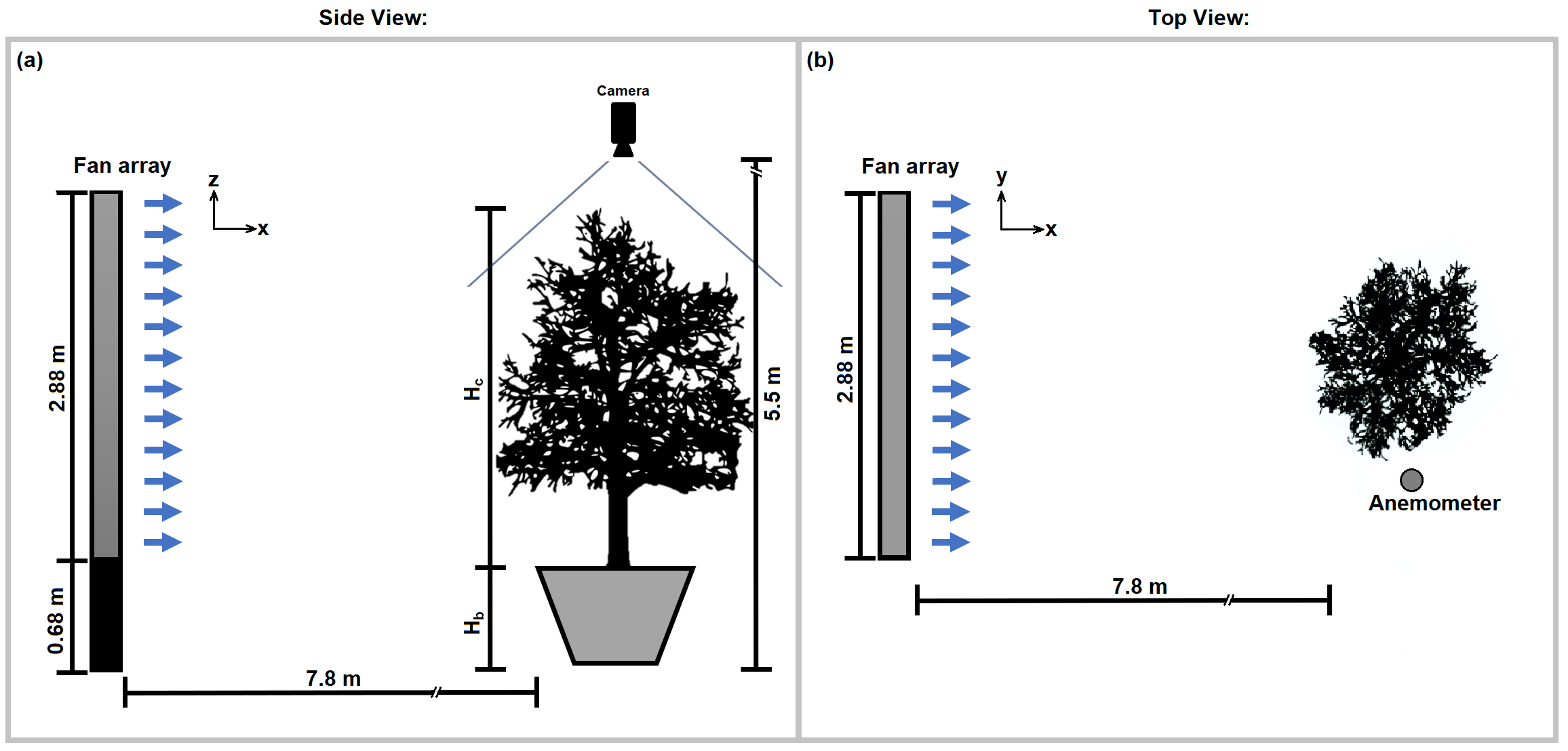
Figure 1: (a) Side view of the experimental setup, including the fan array, example vegetation, and overhead camera (vertical distance and camera size not drawn to scale). $H_{c}$ and $H_{b}$ of each vegetation are detailed in table 1. (b) Top view of the setup, including the fan array, example vegetation, and anemometer.

	$A,$ m2	$\frac{A}{A_{f}}$	$D_{c}$, cm	$\frac{H_{b}}{H_{b_{f}}}$	$H_{c}$, m	Re${}_{\sqrt{A}}\times 10^{-6}$	$S$	TI, %
Oak	04.74 0	00.571 0	08.460	00.860	02.77 0	0.20 – 1.27	00.031 0	21 – 29
Camphor	04.70 0	00.567 0	03.850	00.860	02.57 0	0.34 – 1.24	00.015 0	19 – 25
Bullgrass	00.6220	00.0750	00.180	00.620	00.51 0	0.06 – 0.44	00.00350	27 – 56

Table 1: Vegetation specific parameters describing each species and wind conditions studied. $A$ and $A_{f}$ are vegetation and fan array frontal areas, respectively, $D_{c}$ is trunk diameter, $H_{b}$ and $H_{b_{f}}$ are vegetation and fan array base height, respectively, $H_{c}$ is canopy height, Re is Reynolds number, $S$ is slenderness, and TI is turbulence intensity.

Wind measurements were collected using two anemometers and visual measurements were collected using an overhead camera. The anemometers were placed at 1.8 m and 2.54 m above the ground, respectively. The difference in mean wind speeds measured by the two anemometers was less than the turbulence intensity, and the data from the anemometer at 2.54 m was used for this study. The anemometer measured the streamwise ($x$) and transverse ($y$) wind velocity components at a 4 Hz sampling rate. A color CMOS camera (Campbell Scientific CCFC with image sensor Omnivision OV5653) was installed 5.5 m above the ground, or 175% of the height of the tallest tree, to measure the vegetation from overhead. The camera recorded videos at 15 frames per second with a resolution of 1280 pixels x 720 pixels. Example overhead views at various wind speeds are presented in figure 2. The camera and anemometer were simultaneously triggered by a data logger (Campbell Scientific CR1000X) and each recorded 58-second samples of the wind-vegetation interactions. Thus, each sample consists of 870 frames and 232 two-component (u,v) anemometry measurements. This duration was sufficient to capture variability in the incident wind speed within each sample.

2.2 Analysis

Vegetation displacement fields were computed using PIVlab (Thielicke & Sonntag, 2021), a Matlab based toolbox for particle image velocimetry (PIV), after converting each frame to a monochrome image. An interrogation window size of 16 x 16 pixels with a 50% overlap was used throughout. We manually selected bounding boxes for each sample to only contain the canopy and exclude the tunnel floor in the background. Sample bounding boxes are displayed as dashed black and white rectangles in figure 2. PIV spatial calibration was based on a reference length scale at the height of the top of each canopy. The data were grouped by vegetation species and binned into 1 m/s bins using the wind speed measured by the anemometer located at 2.54 m above the ground.

Temporal statistics of the incident wind are commonly described using two-parameter Weibull distributions for the probability density (Bowden et al., 1983; Tuller & Brett, 1984),

$$f(x)=\begin{cases}\cfrac{k}{\lambda}\left(\cfrac{x}{\lambda}\right)^{k-1}\quad\quad x\geq 0\quad,\\ 0\ \ \quad\quad\quad\quad\quad x<0\quad.\\ \end{cases}$$ (1)

The unbiased maximum likelihood estimator (MLE) of the two parameters, namely, the scale factor $(\lambda)$ and the shape factor $(k)$, are the solution of the simultaneous equations (Bowden et al., 1983),

$$\lambda=\Bigg{[}\Big{(}\cfrac{1}{n}\Big{)}\sum_{i=1}^{n}x_{i}^{k}\Bigg{]}^{\cfrac{1}{k}}\quad,$$ (2)

and,

$$k=\cfrac{n}{\frac{1}{\lambda}\sum_{i=1}^{n}x_{i}^{k}\log{x_{i}}-\sum_{i=1}^{n}\log{x_{i}}}\quad,$$ (3)

where $n$ is the number of samples and $x$ is an observation. We used these equations to describe each sample comprising anemometer measurements of the wind speed and also examined the relevance of this distribution for the vegetation displacement statistics. To assess the fit of the measurements to the Weibull distribution, we computed quantile-quantile (q-q) analyses (Wilk & Gnanadesikan, 1968). Quantiles are defined as continuous intervals resulting from division of the full range of a probability distribution into equal probabilities by ordering the sample data from smallest to largest. Each measurement quantile is compared to the corresponding expected theoretical value. A resulting linear relationship with the theoretical distribution suggests that sampled data likely comes from that distribution.

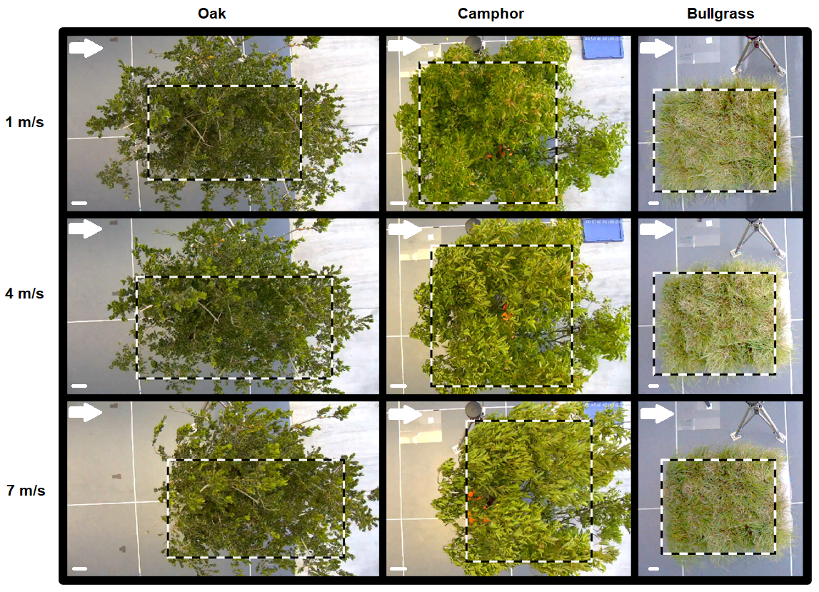
Figure 2: Example overhead views of the vegetation response to three incident wind speeds. The dashed black and white rectangles represent the bounding boxes. The incident wind direction is presented using the white arrows pointing from left to right in each frame. A reference length scale of 0.1 m is marked at the southwest corner of each tile.

3 Results

3.1 Distribution of Wind and Vegetation Speeds

Example probability density functions (PDF) of the wind speed measured in the presence of the vegetation and their corresponding Weibull distribution fits are presented in figure 3(a)-(c). The fit parameters and confidence intervals are summarized in table S1 in the supplementary material. Figure 3(d)-(f) present the q-q curves of the intermediate wind speed distributions. The corresponding low and high wind examples can be seen in figures S1-S3 of the supplementary material. The solid reference lines illustrate the region that corresponds to 75% of the observations, and the resulting linear correlation in the majority of the data suggests the sample data likely comes from the Weibull distribution. The deviation of the data above/below the reference line is only observed in the tails indicating more/less occurrence in the tails than predicted by the theoretical distribution.

Since the wind is the only dynamic load on the vegetation, we compared the distributions of the vegetation displacement speeds with the distributions of the wind speeds. For a more direct comparison with the pointwise wind measurements, the vegetation displacement fields were spatially averaged in each frame. Figure 4 presents PDF, Weibull fits, and q-q curves of the vegetation speeds. The fit parameters can be found in table S1 and q-q curves of the low and high speeds in figures S1-S3, in the supplementary material. As observed in the wind data, the first three quartiles of the vegetation are also linear, indicating a good agreement with the theoretical distribution. A larger deviation from the Weibull distribution, relative to the wind speed measurements, was only observed in the tails of the vegetation speeds. A tendency towards a more linear shape was observed in the vegetation kinematics with an increase in wind speed, indicating the tails of the vegetation displacement distributions are better described by a Weibull distribution at stronger winds.

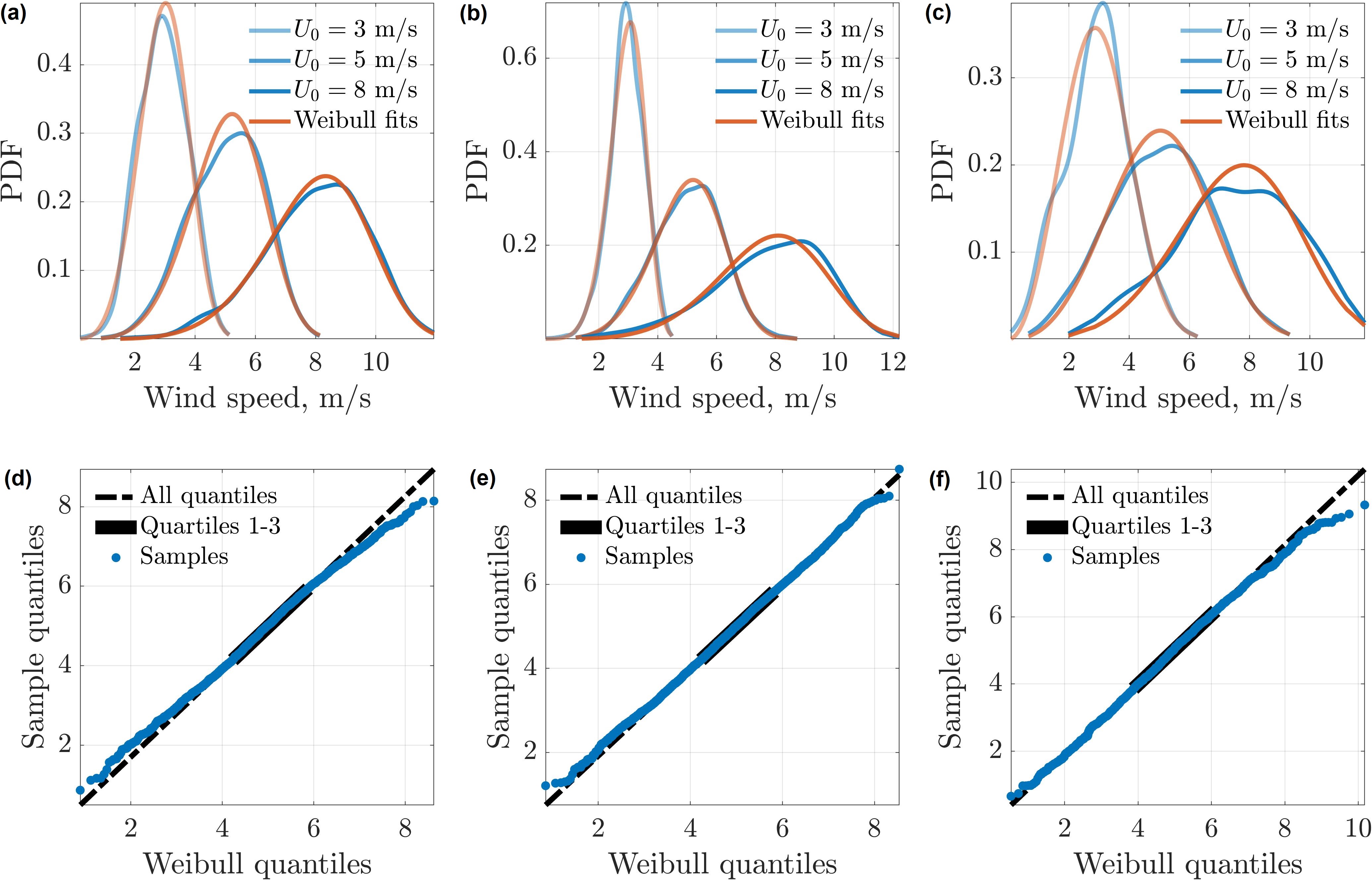
Figure 3: The probability distributions of the wind measured in the presence of the (a) oak, (b) camphor, and (c) bullgrass are shown in blue. Their corresponding Weibull distribution fits are shown in orange. The MLE estimates and confidence intervals of the fits can be found in table S1 of the supplementary material. (d)-(f) Example q-q analyses of the intermediate wind speed observed in (a)-(c), respectively. The solid reference line connects the first and third quartiles, corresponding to 75% of the data, and the dashed reference line extends the solid line to the ends of the samples.

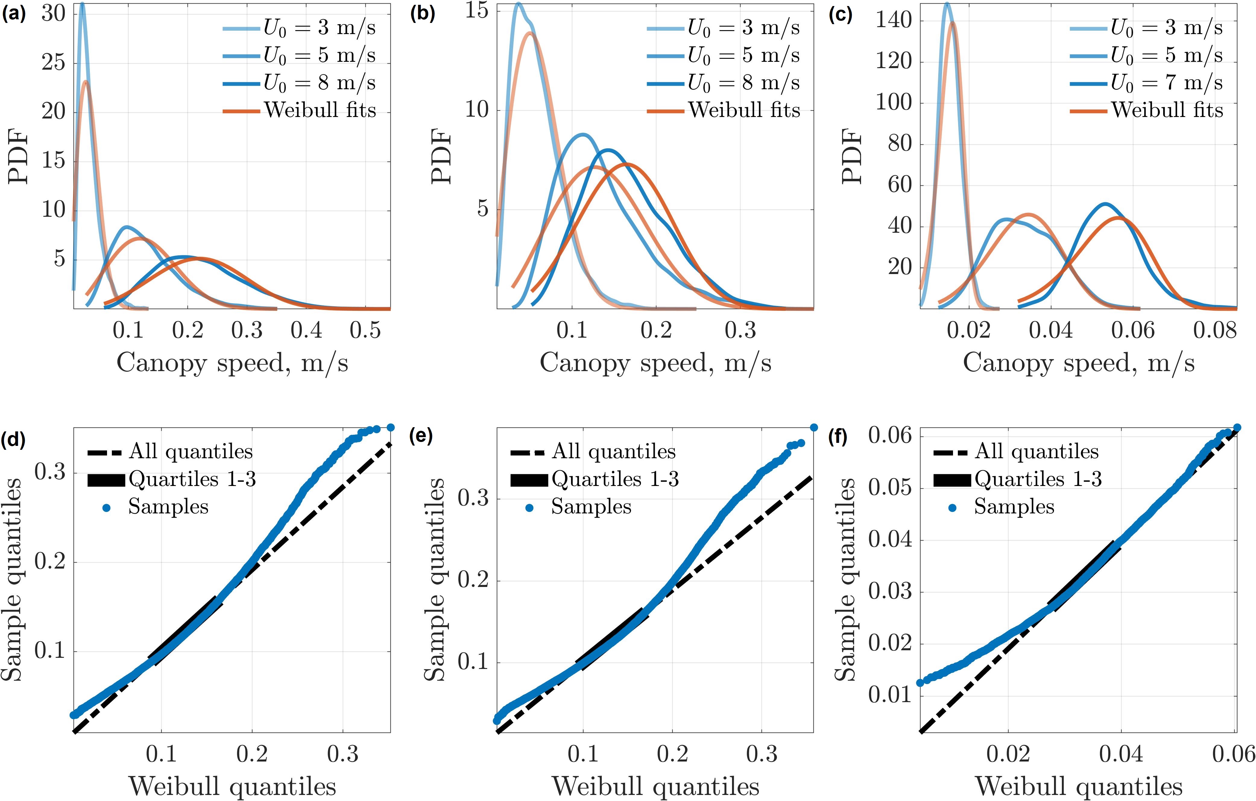
Figure 4: The probability distributions of the vegetation displacement speeds of the (a) oak, (b) camphor, and (c) bullgrass are shown in blue. Their corresponding Weibull distribution fits are shown in orange. The MLE estimates and confidence intervals of the fits can be found in table S1 of the supplementary material. (d)-(f) Example q-q analyses of the intermediate wind speed observed in (a)-(c), respectively. The solid reference line connects the first and third quartiles, corresponding to 75% of the data, and the dashed reference line extends the solid line to the ends of the samples.

3.2 Correlation of Wind and Vegetation Speeds

The relationship between the scale factors of the wind speed, $\lambda_{w}$, and vegetation canopy speed, $\lambda_{c}$ are quantitatively examined in figure 5(a). A three parameter sigmoid function fit was computed for each vegetation using,

$$\lambda_{c}=\cfrac{a}{1+\exp{\bigg{(}\cfrac{-(\lambda_{w}-\lambda_{w_{0}})}{b}\bigg{)}}}\quad,$$ (4)

where $a$ scales the asymptote of the vegetation scale factor in high winds; $\lambda_{w_{0}}$ determines the center of the region of approximately linear response of the vegetation motion with wind speed; and $b$ determines the range of wind speeds over which the vegetation response is approximately linear. The overall R² values are presented in the legend and the fit parameters are available in table 2. Using the fit parameters, we define dimensionless coefficients, $\tilde{\lambda}_{c}=a\lambda_{c}$ and $\tilde{\lambda}_{w}=(\lambda_{w}-\lambda_{w_{0}})/b$, to collapse the data to a single curve,

$$\tilde{\lambda}_{c}=\cfrac{1}{1+\exp{(-\tilde{\lambda}_{w})}}\quad,$$ (5)

as presented in figure 5(b). The sigmoid shape suggests three regimes of vegetation displacement correlation with the flow at low, intermediate, and high wind speeds. The wind and vegetation only exhibit a linear correlation in the intermediate regime, which accordingly limits the use of VA to that regime. It is the region where the scale factor of the wind and vegetation speeds are approximately linearly proportional. In the low- and high-wind regimes, represented by the two plateaus of the sigmoid shape, the vegetation kinematics are insensitive to changes in wind speed. This occurs in the low-wind case because the wind is typically below threshold loading required to displace the vegetation. Higher resilience to wind loading corresponds to vegetation with lower slenderness estimates (Peltola, 1996), and we found that the dimensionless ratio of $\lambda_{w_{0}}/b$ was proportional to the vegetation slenderness estimates (see figure S4 in supplementary material). Conversely, in the high-wind regime, the vegetation becomes maximally deflected, and further increases in wind speed cannot achieve further elastic deformation. Because of these two distinct physical effects, VA cannot be used for accurate wind speed prediction in low- or high-wind regimes. As illustrated in figure 5(a), the quantitative wind speed threshold between sigmoid regimes varies depending on the specific type of vegetation and further exploitation of the sigmoid fit parameters may predict physical properties of the observed structures.

Notably, this sigmoid response shape was previously observed in both data driven and physics based approaches (Cardona et al., 2019, 2021; Cardona & Dabiri, 2022; Sun et al., 2022). Cardona et al. (2019) attributed the errors at the low and high wind regimes to the sampling rate and video duration selection, but the present results suggest a more fundamental physical constraint could be relevant. It is possible, however, that other factors of the kinematics may be present concurrently with the physical limitation revealed here.

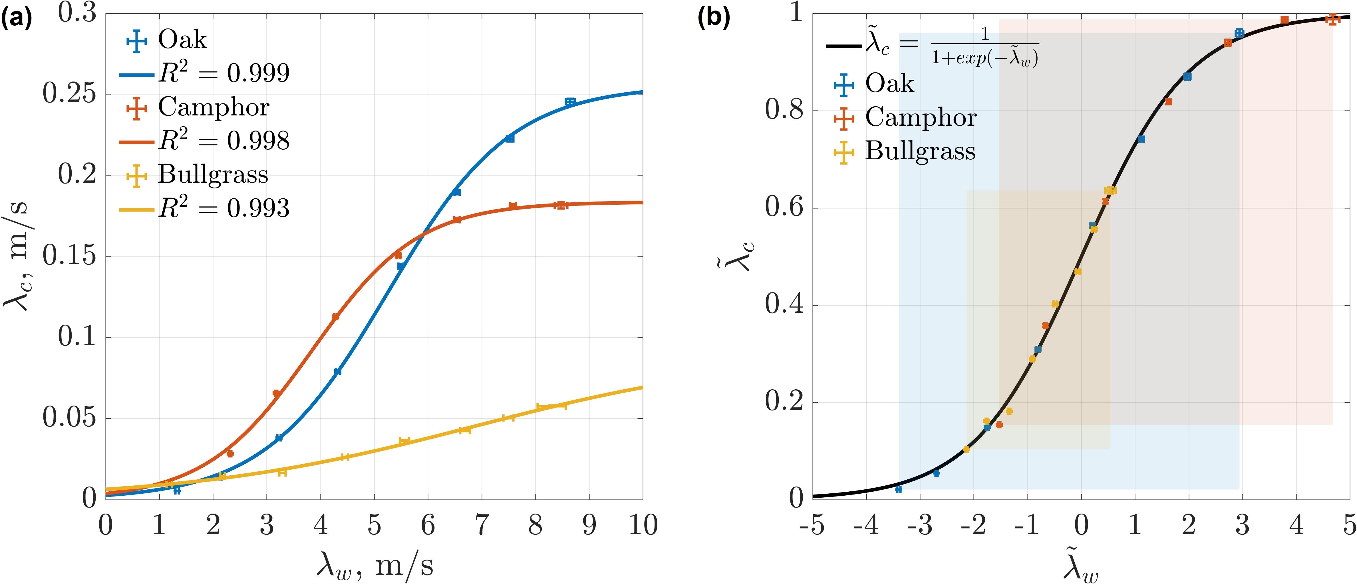
Figure 5: (a) Relationship between the scale factors of the wind speed and vegetation speed. The error bars represent the confidence intervals of the MLE. These scale factor relationships are fit to three parameter sigmoid functions, and the parameters are presented in table 2. (b) Relationship between the dimensionless scale factors. The translucent rectangles of each vegetation demonstrate the range it occupies within the normalized curve.

	$\lambda_{w_{0}}$, m/s	$a$, m/s	$b$, m/s	$\lambda_{w_{0}}/{b}$
Oak	5.250	0.256	1.154	4.55
Camphor	3.836	0.184	0.991	3.87
Bullgrass	6.862	0.091	2.657	2.58

Table 2: The sigmoid function fit parameters of each vegetation. This table corresponds to figure 5(a).

3.3 Inference of Wind Speed and Direction in the Intermediate Wind Regime

Figure 6(a) displays the relationship between the shape factor of the vegetation speeds (i.e. a measure of the distribution breadth) and the scale factor of the wind speeds within the approximately linear regime, i.e. $-1\leq\tilde{\lambda}_{w}\leq 1$. To compare distributions across the three types of vegetation, the shape factor is scaled by $a$ in figure 6(b). The linear regressions revealed similar slopes of $0.044\pm 0.005$ (m/s)^-1 albeit based on only two available wind speeds within the region of linear correlation in the sigmoid profile. The observed similarity in slope across different vegetation types suggests that measurement of the shape factor of the vegetation displacement distribution as well as as a single corresponding wind speed calibration could be sufficient to achieve site-specific VA. Thus, this approach does not eliminate the calibration requirement discussed in the previous studies (Cardona et al., 2019, 2021; Cardona & Dabiri, 2022; Sun et al., 2022), but is robust to achieve complete automation following an initial site specific calibration.

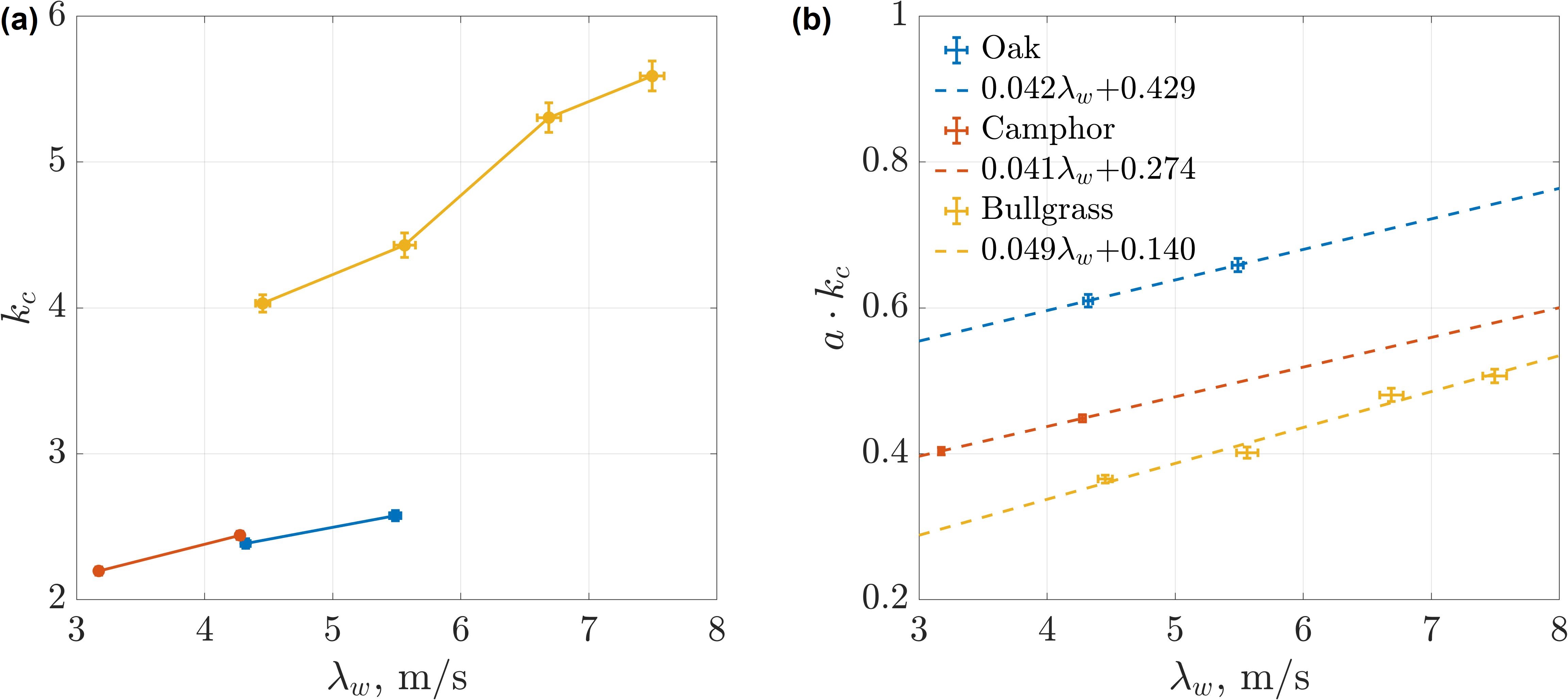
Figure 6: (a) The relationship between the shape factor of the vegetation displacement fields and the scale factor of the wind within the regime of linear proportionality, i.e. $-1\leq\tilde{\lambda}_{w}\leq 1$. (b) The relationship between the non-dimensional shape factor of the vegetation displacement fields and the dimensional scale factor of the wind within the same regime of linear proportionality.

Finally, we propose an approach to infer the direction of the wind. This approach eliminates the aforementioned calibration requirement. Wind direction estimation via VA exploits the fact that the ratio of wind speed components $(u,v)$ can be inferred even if the absolute magnitude of $u$ and $v$ are unknown individually. Here, we compute the average vegetation displacement direction, i.e. $\theta=tan^{-1}(v/u)$, for each frame in a given observation sample. This analysis is conducted on the bullgrass dataset due to the larger number of samples available in the linear range. Figure 7(a) presents the resulting distributions at three sample wind speeds following application of a first order low-pass filter with a cutoff frequency of 1 Hz. Figure 7(b) presents the peak of the distributions for all wind speeds. The distribution peak was selected to avoid potential bias from the tails. The difference in the average direction is less than $1^{\circ}$. Thus, VA is comparable to the sonic anemometer used in this study which has a directional resolution of $1^{\circ}$. Moreover, VA exhibits less variability, likely due to being derived from a 2D field average as opposed to the point-wise anemometer measurement.

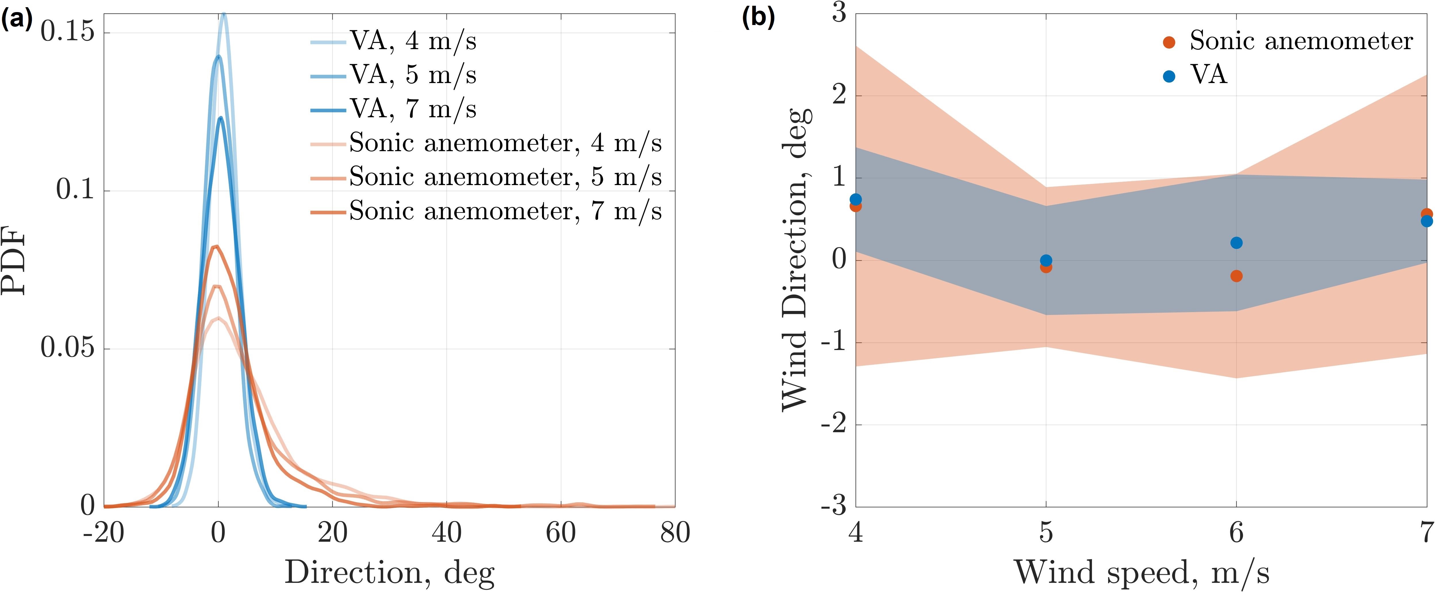
Figure 7: (a) Probability distributions of the wind direction measured using VA and the sonic anemometer. (b) The binned average (circle markers) and standard deviation (transparent bands) of the predicted wind direction within the linear range of proportionality. The difference in the average direction $-0.12^{\circ}\pm 0.24^{\circ}$.

4 Conclusions

The present work has identified the sigmoidal structural response curve as a feature common to three species of vegetation with distinct morphology, size, and material properties. The striking collapse of response data in figure 5(b) suggests that this framework can be used to conceptualize flow-structure interactions in a broader array of vegetation exposed to wind. The three-regime structure of the sigmoid, i.e. at low, intermediate, and high winds, can be understood in terms of vegetation response. At wind speeds below a threshold, vegetation motion shows limited sensitivity to increasing wind. In high winds, a similar insensitivity occurs, but due to distinct physical factors. Here, we observe that the vegetation becomes maximally deflected, with further increases in wind speed unable to achieve further deflection of the vegetation. A region of nearly linear correlation between wind speed and vegetation speed exists. However, quantitative application of VA in the regime requires a priori mapping of the tree kinematics to the corresponding region of the sigmoidal response curve. Hence, at least one point of site-specific calibration appears necessary in order to achieve VA based on vegetation displacement statistics. Future work may endeavor to combine the present physics-based approach with data-driven methods that could infer the sigmoidal response mapping based on a library of other vegetation characteristics, such as the tree species, morphology, age, leaf cover, or other visible physical attributes.

Acknowledgements

The authors gratefully acknowledge M. Fu and N. Esparza-Duran for the assistance with the experiments; S. Anuszczyk, M. Cordeiro, M. Fu, P. Gunnarson, S. Madruga, N. Mohebbi, and N. Wei for watering the plants.

Funding Statement

This work was supported by the National Science Foundation (grant 2019712), Heliogen, and CAST at Caltech.

Declaration of Interests

The authors report no conflict of interest.

Data Availability Statement

The data used in this work will be made available through Mendelay Data.

Author Contributions

Conceptualization: RHG & JOD. Methodology: RHG & JOD. Investigation: RHG. Software: RHG. Data analysis: RHG & JOD. Funding acquisition: JOD & RHG.

Supplementary Material

Additional information can be found in the supplementary material.

References

- Bowden et al. (1983) Bowden, GJ, Barker, PR, Shestopal, VO & Twidell, JW 1983 The weibull distribution function and wind power statistics. Wind Engineering pp. 85–98.
- Cardona et al. (2021) Cardona, Jennifer L., Bouman, Katherine L. & Dabiri, John O. 2021 Wind speed inference from environmental flow–structure interactions. Flow 1, E4.
- Cardona & Dabiri (2022) Cardona, Jennifer L. & Dabiri, John O. 2022 Wind speed inference from environmental flow–structure interactions. part 2. leveraging unsteady kinematics. Flow 2.
- Cardona et al. (2019) Cardona, Jennifer L., Howland, Michael F. & Dabiri, John O. 2019 Seeing the wind: Visual wind speed prediction with a coupled convolutional and recurrent neural network.
- Kinsman (1969) Kinsman, B 1969 Historical notes on the original beaufort scale. Marine Observer 39.
- de Langre (2008) de Langre, Emmanuel 2008 Effects of wind on plants. Annual Review of Fluid Mechanics 40, 141–168.
- Peltola (1996) Peltola, Heli 1996 Swaying of trees in response to wind and thinning in a stand of Scots pine. Boundary-Layer Meteorology 77 (3), 285–304.
- Runia et al. (2019) Runia, Tom F. H., Gavrilyuk, Kirill, Snoek, Cees G. M. & Smeulders, Arnold W. M. 2019 Go with the flow: Perception-refined physics simulation. arXiv preprint .
- Spencer & Shah (2004) Spencer, L. & Shah, M. 2004 Water video analysis.
- Sun et al. (2022) Sun, Jennifer J., Ryou, Serim, Goldshmid, Roni H., Weissbourd, Brandon, Dabiri, John O., Anderson, David J., Kennedy, Ann, Yue, Yisong & Perona, Pietro 2022 Self-supervised keypoint discovery in behavioral videos. In Proceedings of the IEEE/CVF Conference on Computer Vision and Pattern Recognition (CVPR), pp. 2171–2180.
- Thielicke & Sonntag (2021) Thielicke, William & Sonntag, René 2021 Particle image velocimetry for MATLAB: Accuracy and enhanced algorithms in PIVlab. Journal of Open Research Software 9.
- Tuller & Brett (1984) Tuller, Stanton E & Brett, Arthur C 1984 The characteristics of wind velocity that favor the fitting of a weibull distribution in wind speed analysis. Journal of Applied Meteorology and Climatology 23 (1), 124–134.
- Wade & Hewson (1979) Wade, John E & Hewson, Wendell 1979 Trees as local climate wind indicators. Journal of Applied Meteorology 18, 1182–1187.
- Wilk & Gnanadesikan (1968) Wilk, M. B. & Gnanadesikan, R 1968 Probability Plotting Methods for the Analysis of Data. Biometrika 55 (1), 1–17.