Orthogonal and Linear Regressions and Pencils of Confocal Quadrics

Abstract.

This paper enhances and develops bridges between statistics, mechanics, and geometry. For a given system of points in $\mathbb{R}^{k}$ representing a sample of a full rank, we construct an explicit pencil of confocal quadrics with the following properties: (i) All the hyperplanes for which the hyperplanar moments of inertia for the given system of points are equal, are tangent to one of the quadrics from the pencil of quadrics. As an application, we develop regularization procedures for the orthogonal least square method, analogues of lasso and ridge methods from linear regression. (ii) For any given point $P$ among all the hyperplanes that contain it, the best fit is the tangent hyperplane to the quadric from the confocal pencil corresponding to the maximal Jacobi coordinate of the point $P$; the worst fit among the hyperplanes containing $P$ is the tangent hyperplane to the ellipsoid from the confocal pencil that contains $P$. The confocal pencil of quadrics provides a universal tool to solve the restricted principal component analysis restricted at any given point. Both results (i) and (ii) can be seen as generalizations of the classical result of Pearson on orthogonal regression. They have natural and important applications in the statistics of the measurement error models (EIV). For the classical linear regressions we provide a geometric characterization of hyperplanes of least squares in a given direction among all hyperplanes which contain a given point. The obtained results have applications in restricted regressions, both ordinary and orthogonal ones. For the latter, a new formula for test statistic is derived. The developed methods and results are illustrated in natural statistics examples.

1. Introduction

The aim of this paper is to develop further and enhance bridges between three disciplines: statistics, mechanics, and geometry. More precisely, we will explore and employ links between quadrics, moments of inertia, and regressions, in the ordinary linear and the orthogonal settings. This cross-fertilization between the areas appears to be beneficial for each of them. While individual quadrics have been in use in statistics, as reviewed in Section 2 (see also [18, 26]), the novelty of this paper is in the construction of a new object, a confocal pencil of quadrics, associated to a given data set, which we attest to be a powerful and universal tool to study the data. More about confocal pencils of quadrics and associated Jacobi coordinates is given in Section 2 of the Supplementary Material [14], see also e.g. [4], [15].

For a given system of points in $\mathbb{R}^{k}$, under the generality assumption, we construct an explicit pencil of confocal quadrics with the following properties:

(i) All the hyperplanes for which the hyperplanar moments of inertia for the given system of points are equal, are tangent to one of the quadrics from the pencil of quadrics. See Section 3 and Theorem 3.1. As an application, we develop regularization procedures for the orthogonal least square methods, analogues of lasso and ridge methods from linear regression, see Section 3.2. It is based on a dual version of Theorem 3.1, which is given as Theorem 3.2. Another motivation for this study comes from the gradient descent methods in machine learning. An optimization algorithm may not be guaranteed to arrive at the minimum in a reasonable amount of time. As pointed out in e.g. [23] it often reaches some quite low value of the cost function equal to some value $s_{0}$ quickly enough to be useful. Here we deal with the hyperplanar moment as the cost function, in application to the orthogonal least square. From Theorem 3.1, we know that the hyperplanes which generate the hyperpanar moment equal to $s_{0}$ are all tangent to the given quadric from the confocal pencil of quadrics, where the pencil parameter is determined through the value $s_{0}$.

(ii) For any given point $P$ among all the hyperplanes that contain it, the best fit is the tangent hyperplane to the quadric from the confocal pencil corresponding to the maximal Jacobi coordinate of the point $P$. The worst fit among the hyperplanes containing $P$ is the tangent hyperplane to the ellipsoid from the confocal pencil that contains $P$. See Theorem 4.3 from Section 4. We also determine the best and worst fit among $\ell$-dimensional planes containing $P$, for any $\ell:1\leq\ell\leq k-1$, see Section 4 of the Supplementary Material [14].

Both results (i) and (ii) can be seen as generalizations of the classical result of Pearson on orthogonal regression [25], or in other words on the orthogonal least square method (see e.g. [7]). The original result of Pearson is stated below as Theorem 2.1 in Section 2. The original Pearson result also initiated the Principal Component Analysis (PCA), see e.g. [3]. Some of our results have a natural interpretation in terms of PCA, see e.g. Theorem 4.2 from the Supplementary Material [14]. The confocal pencil of quadrics provides a universal tool to solve the Restricted Principal Component Analysis restricted at any given point which we formulate and solve in Section 4, see Theorem 4.1, Corollary 4.1, and Example 4.1. Our generalizations of the Pearson Theorem have natural and important applications in the statistics of the measurement error models, for which the orthogonal regression is known to provide a natural framework, see [7], [20], [6].

We study also the classical linear regression from geometric standpoint, and we do this in a coordinate-free form in Section 5. For the linear regressions we provide a geometric characterization of hyperplanes of least squares in a given direction among all hyperplanes which contain a given point. In the case $k=2$ this is done in Theorem 5.2 and for a general $k$ in Theorem 5.3. The obtained results have applications in restricted regressions, see e.g. [27] for the ordinary linear regressions and see e.g. [20] and [6] for the orthogonal regressions and the measurement error models. Restricted regressions appear in situations with a prior knowledge, which have numerous applications, for example in economics and econometrics, see e.g. [16]. Restricted regressions appear also in tests of hypotheses, see e.g. [27, 16]. For example, assume a system of $N$ points in $\mathbb{R}^{k}$ with the centroid $C$ s given. For the restricted orthogonal regression we derive a new formula for test statistic for the hypothesis that the hyperplane of the best fit contains a given point $P$:

(1.1) $$\frac{N}{N-k+1}(2\lambda_{k_{C}}-\lambda_{k_{P}}),$$

where $\lambda_{k_{P}}$ and $\lambda_{k_{C}}$ are the maximal Jacobi coordinates respectively of the given point $P$ and the centroid $C$, see Theorem 4.4. Here it is assumed that the Jacobi coordinates are induced by the confocal pencil of quadrics associated to the given system of $N$ points. The elegancy of the above formula certifies the appropriateness of the geometric methods and tools developed here for their use in this statistics framework. The developed methods and results are illustrated further in natural statistics settings, see e.g. Examples 4.2 and 5.2. Further studies of statistical properties of the obtained estimators will be conducted in a separate publication.

For the construction of the confocal pencil of quadrics associated to the given system of points, we develop a method based on the study of points with symmetric hyperplanar ellipsoids of inertia. The general $k$-dimensional case is studied in Section 3, which eventually leads to our main result in this direction, Theorem 3.1. For specialization $k=3$ see Example 3.1. from the Supplementary Material [14].

Our method of constructing the confocal pencil of quadrics associated to a given data set combines two main steps: starting from a system of points we consider the central hyperplanar ellipsoid of inertia to whom we attach the points from the line of its major axis, for which the ellipsoid of inertia is symmetric, see Definition 3.2. Then, using the obtained list of the attached points, we assign to them a confocal pencil of quadrics, in accordance to Definition 3.1. The obtained confocal pencil of quadrics does not contain either the hyperplanar ellipsoid of inertia or any of gyrational hyperplanar ellipsoids of inertia. In statistics terminology, the confocal pencil of quadrics does not contain either the ellipsoid of concentration or the ellipsoid of residuals. The confocal pencil does contain, though, a specially normalized axial ellipsoid of gyration. This normalization is not known a priori, and comes only as a consequence of application of our method described above. Let us also note that the idea of considering the points where the ellipsoid of inertia is symmetric is more typical for mechanics than for statistics. A dominant practice in statistics is to consider ellipsoids of concentration or of residuals exclusively centered at the centroid. The cases of given data of a lower rank can be treated similarly, considering subspaces of smaller dimension.

2. Lines and hyperplanes of the best fit to the data set in $\mathbb{R}^{k}$

Nowadays, when we are witnessing the explosion of data science it is important to recall the heroic days of formation of statistics and its mathematical foundations. Ellipses, as two-dimensional quadrics, made a great entrance in statistics in 1886 in the work of Francis Galton [21], which marked the birth of the law of regression.

Galton studied the hereditary transmissions and in [21] he focused on the height. He collected the data of 930 adult children and 205 of their respective parentages. To each pair of parents he assigned a “mid-parent” height, as a weighted average of the heights of the parents. He established the average regression from mid-parent to offsprings and from offsprings to mid-parent. He formulated the law of regression toward mediocrity:

When Mid-Parents are taller than mediocrity, their Children tend to be shorter than they. When Mid-Parents are shorter than mediocrity, their Children tend to be taller than they.

This is how the term regression, thanks to Galton, entered into statistics, although the method of least squares which is in the background, existed in mathematics from the beginning of the XIX century and works of Gauss and Legendre.

In the course of his investigation, Galton discovered a remarkable role of ellipses in analysis of such data. Galton explained in a very nice manner his line of thoughts and actions. We present that in his own words:

“…I found it hard at first to catch the full significance of the entries in the table…They came out distinctly when I ‘smoothed’ the entries by writing at each intersection of a horizontal column with a vertical one, the sum of entries of four adjacent squares… I then noticed that lines drawn through entries of the same value formed a series of concentric and similar ellipses. Their common center … corresponded to $68\frac{1}{4}$ inches. Their axes are similarly inclined. The points where each ellipse in succession was touched by a horizontal tangent, lay in a straight line inclined to the vertical in the ratio of $\frac{2}{3}$; those where they were touched by a vertical tangent lay in a straight line inclined to the horizontal in the ratio of $\frac{1}{3}$. These ratios confirm the values of average regression already obtained by a different method, of $\frac{2}{3}$ from mid-parent to offspring, and of $\frac{1}{3}$ from offspring to mid-parent…These and other relations were evidently a subject for mathematical analysis and verification…I noted these values and phrased the problem in abstract terms such as a competent mathematician could deal with, disentangled from all references to heradity, and in that shape submitted it to Mr. Hamilton Dixson, of St. Peter’s College, Cambridge…

I may be permitted to say that I never felt such a glow of loyalty and respect towards the sovereignty and magnificent sway of mathematical analysis as when his answer reached me, confirming, by purely mathematical reasoning, my various and laborious statistical conclusions with far more minuteness than I had dared to hope… His calculations corrected my observed value of mid-parental regression from $\frac{1}{3}$ to $\frac{6}{17.6}$, the relation between the major and minor axis of the ellipse was changed 3 per cent. (it should be as $\frac{\sqrt{7}}{\sqrt{2}}$)…”

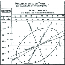
Figure 1. From [21].

In his seminal paper [25], one of the founding fathers of modern statistics, Karl Pearson, investigated the question of the hyper-plane which minimizes the mean square distance from a given set of points in $\mathbb{R}^{k}$, for any $k\geq 3$. In his own words, Pearson formulated the problem: “In the case we are about to deal with, we suppose the observed variables–all subject to error–to be plotted in plane, three-dimensioned or higher space, and we endeavour to take a line (or plane) which will be the ‘best fit’ to such a system of points. Of course the term ‘best fit’ is really arbitrary; but a good fit will clearly be obtained if we make the sum of the squares of the perpendiculars from the system of points upon the line or plane a minimum.”

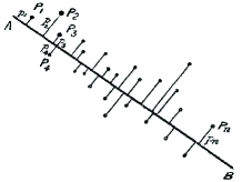
Figure 2. From [25].

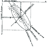
Figure 3. From [25].

Thus, the notion of the best fit is not uniquely determined. In statistics, the choice of the squares of the perpendiculars is natural in the measurement error models, or in other words in regression with errors in variables (EIV), [7]. This corresponds to Pearson’s above remark “we suppose the observed variables–all subject to error”. In such models it is assumed that both predictors and responses are known with some error. In contrast to that, in the classical linear regressions, mentioned above, it is assumed that only responses are known with some error, while for the predictors the exact values are known. Thus, the squares of distances along one of the axes is in use in such classical regression models, see also Section 5.2 and Example 6.1 from the Supplementary Material [14]. We will call that directional regression in a given direction. We will talk more about its geometric aspects in the last Section 5.

Let us make a more rigorous definitions of the classical simple linear regression model and regression with error in variables (EIV) models, [7]. For classical simple regression model, it is assumed that the values $(x^{(i)})_{i=1}^{N}$ are known, fixed values, as for example values set up in advance in the experiment. The values $(y^{(i)})_{i=1}^{N}$ are observed values of uncorrelated random variables $Y_{i}$, $i=1,\dots,N$ with the same variance $\sigma^{2}$. There is a linear relationship assumed between the predictors $x^{(i)}$ and responses $(y^{(i)})_{i=1}^{N}$: $EY_{i}=\alpha+\beta x^{(i)},\quad i=1,\dots,N.$ This can be restated as $Y_{i}=\alpha+\beta x^{(i)}+\epsilon_{i},\quad i=1,\dots,N,$ where $\epsilon_{i}$ are called the random errors and they are uncorrelated random variables with zero expectation and the same variance $\sigma^{2}$. In such models the regression is of $Y$ on $x$, i.e. in the vertical direction, see Example 6.1 from the Supplementary Material [14]. This model was in the background of the Galton study [21], mentioned above.

There are also important situations where predictors are known only up to some error and they are described by measurement error models. There the observed pairs $(x^{(i)},y^{(i)})_{i=1}^{N}$ are sampled from random variables $(X_{i},Y_{i})$ with means satisfying the linear relationship $EY_{i}=\alpha+\beta(EX_{i}),\quad i=1,\dots,N.$ Denoting $EX_{i}=\xi_{i}$, the errors in variables model can be defined as $Y_{i}=\alpha+\beta\xi_{i}+\epsilon_{i},\quad X_{i}=\xi_{i}+\delta_{i},\quad i=1,\dots,N,$ where both $X_{i}$ and $Y_{i}$ have error terms which belong to mean zero normal distributions, such that all $\epsilon_{i}$, $i=1,\dots,N$ have the same variance $\sigma^{2}_{\epsilon}$ and all $\delta_{i}$, $i=1,\dots,N$ have the same variance $\sigma^{2}_{\delta}$. Since in such models there is a symmetry between $x_{i}$ and $y_{i}$ as they are both known with an error, it is more natural to apply to them the orthogonal regression, or in other words, the orthogonal least square method. This we are going to introduce next under the assumption that $\eta=\sigma^{2}_{\epsilon}/\sigma^{2}_{\delta}=1$ and in a general dimension $k$. One should also mention that applications of the orthogonal least square method in the models with measurement errors have limitations, see e.g. [6], [5]. These limitations are related to a potentially unknown value of $\eta$. Here we assume that $\eta$ is known. At first we assume that $\eta=1$. The assumption that $\eta$ is known is essential, while that it is equal to one is not, as we will show later, see Remark 4.1.

From a historic perspective, the case $\eta=1$ originated from [1, 2]. Then it was Pearson who established orthogonal regression by selecting the squares of the perpendiculars, which corresponds to the case $\eta=1$. Nowadays, it is also called the orthogonal least square method, see e.g. [7], as mentioned above. The geometric aspects of the orthogonal regression are the main subject of this study. We also adopt the Pearson’s generality assumption, that the given system of points does not belong to a hyper-plane.

To fix the idea, suppose the system of $N$ points $(x_{1}^{(i)},x_{2}^{(i)},\dots,x_{k}^{(i)})_{i=1}^{N}$ is given. Define the centroid, or the mean values of the coordinates $\bar{x}_{j}$ and the variances $\sigma^{2}_{x_{j}}$:

$$\bar{x}_{j}=\frac{1}{N}\sum_{i=1}^{N}x_{j}^{(i)},\quad\sigma^{2}_{x_{j}}=\frac{1}{N}\sum_{i=1}^{N}(x_{j}^{(i)}-\bar{x}_{j})^{2},\quad j=1,\dots,k.$$

Due to the generality assumption, all $\sigma^{2}_{x_{j}}$, for $j=1,\dots,k$ are non-zero. Then, the correlations $r_{jl}$ and the covariances $p_{jl}$ are

$$r_{jl}=\frac{p_{jl}}{\sigma_{x_{j}}\sigma_{x_{l}}},\,p_{jl}=\frac{1}{N}\sum_{i=1}^{N}(x_{j}^{(i)}-\bar{x}_{j})(x_{l}^{(i)}-\bar{x}_{l}),\quad j,l=1,\dots,k,l\neq j.$$

The covariance matrix $K$ is a $(k\times k)$ matrix with the diagonal elements $K_{jj}=\sigma^{2}_{x_{j}},j=1,\dots,k,$ and the off-diagonal elements $K_{jl}=p_{jl},j,l=1,\dots,k,l\neq j.$ The covariance matrix is always symmetric positive semidefinite. However, here we have more: $K$ is a positive-definite matrix due to the generality assumption. In particular, it has the inverse $K^{-1}$ and all its eigenvalues are positive. Pearson defined the ellipsoid of residuals by the equation

$$\sum_{j,l=1}^{k}K_{jl}x_{j}x_{l}=const.$$

Denote the eigenvalues of $K$ as $\mu_{1}\geq\dots\geq\mu_{k}>0$.

Theorem 2.1.

[Pearson, [25]] The minimal mean square distance from a hyperplane to the given set of $N$ points is equal to the minimal eigenvalue of the covariance matrix $K$. The best-fitting hyperplane contains the centroid and it is orthogonal to the corresponding eigenvector of $K$. Thus, it is the principal coordinate hyperplane of the ellipsoid of residuals which is normal to the major axis.

Then Pearson studied the lines which best fit to the given set of points and proved

Theorem 2.2.

[Pearson, [25]] The line which fits best the given system of $N$ points contains the centroid and coincides with the minor axis of the ellipsoid of residuals.

Pearson integrated the visualization of the linear regression with the orthogonal regression in the planar case in [25] in Fig. 3. The ellipse in Fig. 3 is dual to the ellipse of residuals and it coincides with the object studied by Galton. The main goals of this paper are to generalize the above classical results of Pearson in the following directions.

The first goal: For a given system of $N$ points in $\mathbb{R}^{k}$, for any $k\geq 2$, under the generality assumption, we consider all hyperplanes which equally fit to the given system of points. In other words, for any fixed value $s$ not less than the smallest eigenvalue $\mu_{k}$ of the covariance matrix $K$, we consider all hyperplanes for which the mean sum of square distances to the given set of points is equal to $s$. Starting from the ellipsoid of residuals, we are going to effectively construct a pencil of confocal quadrics with the following property: For each $s\geq\mu_{k}$ there exists a quadric from the confocal pencil which is the envelope of all the hyperplanes which $s$-fit to the given system of points.

We stress that the ellipsoid of residuals does not belong to the confocal family of quadrics. The construction of this confocal pencil of quadrics is fully effective, though quite involved. The obtained pencil of confocal quadrics is going to have the same center as the ellipsoid of residuals and moreover, the same principal axes.

Example 2.1.

Let us recall that $\mu_{k}$ denotes the smallest eigenvalue of the covariance matrix $K$. In the case $s=\mu_{k}$ there is only one hyperplane which $s$ fits to the given set of $N$ points. This is the best-fitting hyperplane described in Theorem 2.1. The envelope of this single hyperplane is this hyperplane itself. This hyperplane is going to be a degenerate quadric from our confocal pencil of quadrics.

The second goal: For a given system of $N$ points in $\mathbb{R}^{k}$, for any $k\geq 2$, under the generality assumption, find the best fitting hyperplane under the condition that they contain a selected point in $\mathbb{R}^{k}$. We also provide an answer to the questions of the best fitting line and more general the best fitting affine subspace of dimension $\ell$, $1\leq\ell\leq k-1$ under the condition that they contain a given point.

A careful look at the Galton’s figure (see Fig. 1) discloses an intriguing geometric fact that the line of linear regression of $y$ on $x$ intersects the ellipse at the points of vertical tangency, while the line of linear regression of $x$ on $y$ intersects the ellipse at the points of horizontal tangency. Further analysis of this phenomenon leads us to our third goal.

The third goal: to study linear regression in $\mathbb{R}^{k}$ in a coordinate free, invariant, form, see Theorem 5.3 and Corollary 5.3. We address the following question: for a given direction and a given system of $N$ points under the generality assumption, what is the best fitting hyperplane in the given direction, among those that contain a selected point in $\mathbb{R}^{k}$?

Apparently, the second and the third goal are addressed using the same confocal pencil of quadrics constructed in relation with the first goal and mentioned above.

Let us conclude the introduction by observing that the ellipsoids reciprocal to the Pearson ellipsoid of residuals, called the concentration ellipsoids or the data ellipsoids have been studied in statistics, see e.g. [10]. The equation of the data ellipsoid related to the above ellipsoid of residuals is:

$$\sum_{j,l=1}^{k}K^{-1}_{jl}x_{j}x_{l}=const.$$

As it was shown in [10], this ellipsoid has the same first and second moments about the centroid as the given set of points. The above Pearson results can be naturally restated in terms of the concentration ellipsoid as well. In particular, in two-dimensional case, the Galton ellipses are examples of concentration ellipsoids and they are, as we mentioned above, dual to ellipses of residuals of Pearson. The ellipsoids of concentration in two-dimensional case are naturally called the ellipses of concentration; they are presented in Fig. 1 and 3.

The notions of moments in statistics came from mechanics, where they were originally introduced in the three-dimensional space. We are going to review these basic notions from a mechanics perspective in Section 1 of the Supplementary Material [14].

3. The envelopes of hyperplanes which equally fit the data in $k$-dimensional case

In this Section we construct a pencil of confocal quadrics associated to a system of points in $\mathbb{R}^{k}$. This pencil of confocal quadrics is going to be instrumental in reaching of all three of our main goals as listed in Section 2. In Section 3.1 we present two main steps in our method of constructing the confocal pencil of quadrics: starting from a system of points we consider the central hyperplanar ellipsoid of inertia to whom we attach the points for which the ellipsoid of inertia is symmetric, see Definition 3.2. Then, using the obtained list of the attached points, we assign to them a confocal pencil of quadrics, in accordance to Definition 3.1.This eventually leads to the main result in this direction, Theorem 3.1. The three-dimensional case will be presented in Example 3.1 of the Supplementary Material [14].

In Section 3.2, we deal with the first applications of Theorem 3.1 in the regularization for orthogonal regression and in the gradient descent method in machine learning. The initial step is a dual formulation of Theorem 3.1 which is given as Theorem 3.2. Then, methods of regularization for orthogonal regression, which are analogues of the lasso and the ridge for linear regression, are presented.

So far, we dealt with axial and hyperplanar moments of inertia. In Section 4 of the Supplementary Material [14], we introduce a general concept of $\ell$-planar moments in $\mathbb{R}^{k}$, for all $1\leq\ell\leq k-1$. Then axial and hyperplanar moments correspond to $\ell=1$ and $\ell=k-1$ respectively. We connect the construction of $\ell$ planar moments with PCA.

3.1. Construction of the confocal pencil of quadric associated to the data in $\mathbb{R}^{k}$

Let the system of points $M_{1},...,M_{N}$ with masses $m_{1},...,m_{N}$ be given in $\mathbb{R}^{k}$. Consider a hyperplane $\pi$ in the same space $\mathbb{R}^{k}$. The hyperplanar moment of inertia for the system of points for the hyperplane $\pi$ is, by definition: $J_{\pi}=\sum\limits_{i=1}^{N}m_{i}d_{i}^{2}.$

The generalization of the Huygens-Steiner theorem is valid here: $J_{\pi}=J_{\pi_{1}}+md^{2},$ where it is assumed that the hyperplane $\pi$ contains the center of masses, while $\pi_{1}$ is a hyperplane parallel to $\pi$ at the distance $d$. Here $m$ is the total mass of the system of points. The hyperplanar operator of inertia is defined here as a $k$-dimensional symmetric operator as follows: $\langle J_{O}\mathbf{n_{1}},\mathbf{n_{2}}\rangle=\sum\limits_{j=1}^{N}m_{j}\langle\mathbf{r_{j}},\mathbf{n_{1}}\rangle\langle\mathbf{r_{j}},\mathbf{n_{2}}\rangle,$where $\mathbf{r_{j}}$ is the radius vector of the point $M_{j}$. We see that $J_{\pi}=\langle J_{O}\mathbf{n},\mathbf{n}\rangle,$ where $\mathbf{n}$ is the unit vector orthogonal to the hyperplane $\pi$. In a principal basis, i.e. one where the hyperplanar operator of inertia has a diagonal form, the diagonal elements are the moments of inertia of the coordinate hyperplanes:

$$J_{1}=\sum\limits_{j=1}^{N}m_{j}x_{1j}^{2},\,J_{2}=\sum\limits_{j=1}^{N}m_{j}x_{2j}^{2},\,\dots,\,J_{k}=\sum\limits_{j=1}^{N}m_{j}x_{kj}^{2}.$$

Definition 3.1.

Let a $(k-1)$-dimensional ellipsoid

(3.1) $$\frac{x_{1}^{2}}{\alpha_{1}}+...+\frac{x_{k}^{2}}{\alpha_{k}}=1,$$

with $\alpha_{1}>...>\alpha_{k}>0$ be given. We say that the set of $2k-2$ collinear points $F_{1i}(\sqrt{\alpha_{1}-\alpha_{i}},\allowbreak 0,...,0)$, $F_{2i}(-\sqrt{\alpha_{1}-\alpha_{i}},0,...,0)$, $i=2,...,k$, organized in $(k-1)$ pairs of points symmetric with respect to one given point is assigned to the ellipsoid (3.1).

All these assigned points belong to the coordinate axis $Ox_{1}$ that contains the major semi-axis of the ellipsoid. Important properties of the points with symmetric ellipsoid of inerta will be presented elsewhere [13].

Suppose that the principal moments of inertia satisfy $0<J_{1}<J_{2}<...<J_{k}$. Let us define $a^{2}_{2},a^{2}_{3},...,a^{2}_{k}$ by $J_{1}+ma_{2}^{2}=J_{2},\quad J_{1}+ma_{3}^{2}=J_{3},...,J_{1}+ma_{k}^{2}=J_{k}.$ From the last formulas, we get

(3.2) $$J_{1}=J_{k}-ma_{k}^{2},\,J_{2}=J_{k}+ma_{2}^{2}-ma_{k}^{2},\dots,J_{k-1}=J_{k}+ma_{k-1}^{2}-ma_{k}^{2}.$$

Definition 3.2.

For the hyperplanar ellipsoid of inertia

(3.3) $$J_{1}x_{1}^{2}+...+J_{k}x_{k}^{2}=1$$

let us attach the points $F_{1i}(a_{i},0,...,0)$ and $F_{2i}(-a_{i},0,...,0)$, for $i=2,...,k$, where $\pm a_{i}$ are determined from (3.2), characterized by the following property: They are the points of the line of the major axis of the central ellipsoid of inertia, where two principal moments of inertia coincide, in other words, these are the points for which the hyperplanar ellipsoid of inertia is symmetric.

Now, let us construct the confocal pencil of quadrics for which these points attached to the hyperplanar ellipsoid of inertia are assigned points in the sense of Definition 3.1:

(3.4) $$\frac{x_{1}^{2}}{\frac{J_{1}}{m}-\lambda}+\frac{x_{2}^{2}}{\frac{J_{1}}{m}-a_{2}^{2}-\lambda}+...+\frac{x_{k}^{2}}{\frac{J_{1}}{m}-a_{k}^{2}-\lambda}=1.$$

Thus, we construct the pencil of confocal quadrics (3.4) starting from the hyperplanar ellipsoid of inertia (3.3) in a highly nontrivial way: we first attach points with a symmetric ellipsoid of inertia and then, assign to them the confocal pencil of quadrics. The obtained confocal pencil of quadrics has a remarkable property with respect to the initial system of points which defined the hyperplanar ellipsoid of inertia.

Theorem 3.1.

Given a system of points in $\mathbb{R}^{k}$ of the total mass $m$ with the principal hyperplanar moments of inertia $0<J_{1}<J_{2}<\dots<J_{k}$ with the center of masses $C$. Consider the family of hyperplanes for which the system of points has the same hyperplanar moment of inertia. All hyperplanes from the family are tangent to the same quadric from the pencil of confocal quadrics (3.4), which can be reparametrized as

(3.5) $$\frac{x_{1}^{2}}{A^{2}}+\frac{x_{2}^{2}}{A^{2}-a_{2}^{2}}+...+\frac{x_{k}^{2}}{A^{2}-a_{k}^{2}}=1.$$

The type of the enveloping quadric depends on the value of the parameter $A$. Here $J_{\pi}=J_{k}+mS_{k}=J_{k}+m(A^{2}-a_{k}^{2})$, or $A^{2}=\frac{J_{\pi}-J_{1}}{m}.$From the last formula it follows that hyperplanes with hyperplanar moment of inertia equal to $J_{\pi}$ are tangent to the following quadric from the confocal pencil (3.4):

(3.6) $$\frac{x_{1}^{2}}{J_{\pi}-J_{1}}+\frac{x_{2}^{2}}{J_{\pi}-J_{2}}+...+\frac{x_{k}^{2}}{J_{\pi}-J_{k}}=\frac{1}{m}.$$

Thus, in terms of the value of the hyperplanar moment of inertia $J_{\pi}$ one gets the following information about the type of the enveloping quadric:

• If $J_{\pi}>J_{k}$, then the enveloping quadric is a $k$-dimensional ellipsoid.

• If $J_{i}<J_{\pi}<J_{i+1}$, then the enveloping quadric belongs to the $i$-th type quadrics.

• In the case $J_{\pi}<J_{1}$, there is no hyperplane with the hyperplanar moment of inertia equal to $J_{\pi}$.

• If $J_{\pi}=J_{i}$, for any $i=1,\dots,k$, then the enveloping quadric is degenerate and the hyperplane $\pi$ coincides with the enveloping quadric, as a coordinate hyperplane.

The proof of Theorem 3.1 is given in Section 3 of the Supplementary Material [14] followed by Example 3.1, which specializes the three-dimensional case. A trace of the statement of Theorem 3.1 in three-dimensional case can be retrieved from [22]. However, the presentation in [22] was very vague and unusual even for the standards of that historic period. It was written more like a report or an essay rather than as a scientific paper, since it did not provide clear statements, formulas, or proofs of the main assertions.

3.2. Applications in the regularization of the orthogonal least square method

Using duality between quadrics of points and quadrics of tangential hyperplanes, we can reformulate the above Theorem 3.1 as follows:

Theorem 3.2.

Given a system of points in $\mathbb{R}^{k}$ of the total mass $m$ with the principal hyperplanar moments of inertia $0<J_{1}<J_{2}<\dots<J_{k}$ with the center of masses $C$. Consider the family of hyperplanes for which the system of points has the same hyperplanar moment of inertia. All the hyperplanes from the family form a quadric. By varying the hyperplanar moment of inertia the obtained quadrics form a linear pencil dual to the confocal pencil (3.4).

This dual formulation can be used to study nonlinear constraints on the hyperplanes of regression. Such situations may arise in regularization problems for the orthogonal least square method. In the case of the regularization of the standard linear regression, there are various shrinkage methods developed (see e.g. [24]). For example the ridge or the lasso methods depend on the type of the norm used to bound the coefficients of the hyperplanes. Here we develop similar methods for the orthogonal least square. A ridge-type method imposes an $L_{2}$ bound on the coefficients $\beta_{1},\dots,\beta_{k}$ of the hyperplanes: $||\beta||_{2}\leq s.$ A lasso-type method assumes use of the $L_{1}$ norm and the condition on the coefficients $\beta_{1},\dots,\beta_{k}$ of the hyperplanes can be written as: $||\beta||_{1}\leq t.$ The best-fit hyperplane under each of these conditions is determined as the point of tangency of a quadric from the linear pencil from Theorem 3.2 and the $L_{2}$ circle of radius $s$ in the first case and the $L_{1}$ circle (akka the diamond) of radius $t$ in the second case, see Fig. 4.

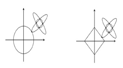
Figure 4. Regularization for the orthogonal least square method: to the left, $L_{2}$ or ridge-type case; to the right, $L_{1}$ or lasso-type case. See Remark 3.1.

The situation of the lasso and ridge in the classical linear regression was presented on Fig. 3.11 in [24]. The differences between these regularizations in the linear regression case vs. the orthogonal least square case are:

1. in the linear regression the family of quadrics present a family of homothetic quadrics defined by equation (3.51) from [24], while in the orthogonal least square situation developed here uses a linear pencil of quadrics from Theorem 3.2;

2. the free term $\beta_{0}$ was not included in bounding the $\beta$ coefficients in the linear regression and in the orthogonal least square case bounding includes all $\beta$’s;

3. in the linear regression case the obtained regularized hyperplane contains the center of masses, while in the orthogonal least square this is not the case.

Remark 3.1.

A linear pencil of quadrics is generated by two quadrics. In the planar case, a linear pencil of conics is generated by two conics, see Fig. 4. A generic linear pencil of conics consists of all conics which share four common points, see e.g. [15].

Another application of the methods developed in this paper is related to the gradient descent in the machine learning. The optimization algorithm may not be guaranteed to arrive at the minimum in a reasonable amount of time. But, as noted in [23], it often reaches some quite low value of the cost function (here the hyperplanar moment) equal to $s_{0}$ quickly enough to be useful. In application to the orthogonal least square, from Theorem 3.1, we know that the hyperplanes which generate the hyperplanar moment equal to $s_{0}$ are all tangent to the given quadric from the pencil (3.4); the pencil parameter is determined through $s_{0}$.

4. Hyperplanes containing a given point which best fit the data in $\mathbb{R}^{k}$. Restricted PCA

As a further employment of the confocal pencil of quadrics which we constructed in Section 3.1, associated to a given system of points in $\mathbb{R}^{k}$, see Theorem 3.1, we are going to reach our second goal as listed in Section 2. We also formulate and solve the Restricted PCA, restricted at a point, using the same confocal pencil of quadrics as a universal tool, see Theorem 4.1. In Example 4.2, we apply the developed methods in a natural situation of an errors-in-variables model. We show how it effectively works in testing a hypothesis that the line of the best fit contains a given point. We derive a new formula for test statistics in restricted orthogonal least square method in Theorem 4.4.

Let the system of points $M_{1},...,M_{N}$ with masses $m_{1},...,m_{N}$ be given in $\mathbb{R}^{k}$ and let $C$ be the center of masses. We consider the following problem: For a given point $P(x_{01},...,x_{0k})$ in $\mathbb{R}^{k}$ find the principal hyperplanes of the hyperplanar ellipsoid of inertia.

The family of confocal quadrics (3.4) which we associated with the given system of points, provides the solution to the above problem in the following way. Assume that the principal axes at the point $C$ are chosen as the coordinate axes. Let the hyperplane $\pi$ containing the point $P$ be given, with $\mathbf{n}=(n_{1},n_{2},...,n_{k})$, as the unit normal vector to the hyperplane. Using the Hygens-Steiner’s theorem, the moment of inertia for the hyperplane $\pi$ is $J_{\pi}=J_{\pi_{C}}+md^{2},$ where $J_{\pi_{C}}$ is the moment of inertia for the hyperplane $\pi_{C}$, where $\pi_{C}$ contains the center of masses $C$ and is parallel to the hyperplane $\pi$. Let $d$ be the distance from $C$ to $\pi$. The square of the distance is given by formula $d^{2}=(x_{01}n_{1}+...+x_{0k}n_{k})^{2}.$ One has $J_{\pi}=J_{1}n_{1}^{2}+...+J_{k}n_{k}^{2}+md^{2}=J_{1}n_{1}^{2}+...+J_{k}n_{k}^{2}+m(x_{01}n_{1}+...+x_{0k}n_{k})^{2}.$ The direction of the principal axes at the point $P$ can be obtained as the stationary points of the function $J_{\pi}(n_{1},...,n_{k})$. Since $n_{1}^{2}+...+n_{k}^{2}=1$, the stationary points can be obtained using the Lagrange multipliers. As usual, consider the function

(4.1) $$F(n_{1},...,n_{k},\mu)=J_{1}n_{1}^{2}+...+J_{k}n_{k}^{2}+m(x_{01}n_{1}+...+x_{0k}n_{k})^{2}-\mu(n_{1}^{2}+...+n_{k}^{2}-1),$$

where $\mu$ is the Lagrange multiplier. We get the stationary points from the condition that the partial derivatives of $F$ are equal to zero. One gets the system:

(4.2) $$(J_{P}-\mu E)\mathbf{n}=0,\quad n_{1}^{2}+...+n_{k}^{2}-1=0,$$

where $J_{P}$ is the planar inertia operator at the point $P$, given by

(4.3) $$J_{P}=\left(\begin{matrix}J_{1}+mx_{01}^{2}&mx_{01}x_{02}&...&mx_{01}x_{0k}\\ mx_{02}x_{01}&J_{2}+mx_{02}^{2}&...&mx_{02}x_{0k}\\ .&&&\\ .&&&\\ .&&&\\ mx_{0k}x_{01}&mx_{0k}x_{02}&...&J_{k}+mx_{0k}^{2}\end{matrix}\right).$$

The first part in (4.2) is a homogeneous system of $k$ equations in $n_{1},...,n_{k}$ with $\mu$ as a parameter. The nontrivial solutions exist under the condition that the determinant of the system vanishes. This determinant is equal to the characteristic polynomial of the symmetric matrix $J_{P}$, with roots $\mu_{1},...,\mu_{k}$ being the eigenvalues of the matrix $J_{P}$. They are the principal planar moments of inertia at the point $P$. Each eigenvalue $\mu_{j}$ has a corresponding eigenvector $\mathbf{n}_{{j}}$, which is the unit normal vector of a principal hyperplane. Since $J_{P}$ is symmetric, all eigenvalues are real, and corresponding eigenvectors $\mathbf{n}_{(1)},...,\mathbf{n}_{(k)}$ are mutually orthogonal.

Let us look at the system (4.2) in another way. First $k$ equations can be rewritten as:

$$\frac{mx_{01}}{\mu-J_{1}}=\frac{n_{1}}{n_{1}x_{01}+...+n_{k}x_{0k}},\quad\dots,\quad\frac{mx_{0k}}{\mu-J_{k}}=\frac{n_{k}}{n_{1}x_{01}+...+n_{k}x_{0k}}.$$

By multiplying $j$-th equation by $x_{0j}$ and adding all of them, we come to the confocal pencil of quadrics:

(4.4) $$\frac{x_{01}^{2}}{\mu-J_{1}}+\frac{x_{02}^{2}}{\mu-J_{2}}+...+\frac{x_{0k}^{2}}{\mu-J_{k}}=\frac{1}{m}.$$

Each eigenvalue $\mu_{j}$ of the matrix $J_{P}$ corresponds to one quadric from (4.4) which passes through the point $P$. Denote by $X_{P}$ the $N\times k$ matrix of the data related to the point $P$

$$X_{P}=\left(\begin{matrix}\sqrt{m_{1}}(x_{1}^{(1)}-x_{01})&\sqrt{m_{2}}(x_{1}^{(2)}-x_{01})&...&\sqrt{m_{N}}(x_{1}^{(N)}-x_{01})\\ \sqrt{m_{1}}(x_{2}^{(1)}-x_{02})&\sqrt{m_{2}}(x_{2}^{(2)}-x_{02})&...&\sqrt{m_{N}}(x_{2}^{(N)}-x_{02})\\ .&&&\\ .&&&\\ .&&&\\ \sqrt{m_{1}}(x_{k}^{(1)}-x_{0k})&\sqrt{m_{2}}(x_{k}^{(2)}-x_{0k})&...&\sqrt{m_{N}}(x_{k}^{(N)}-x_{0k})\end{matrix}\right).$$

Here $(x_{1}^{(j)},\dots,x_{k}^{(j)})$ denotes the coordinates of the point $M_{j}$, for $j=1,\dots,N.$ We have $J_{P}=X_{P}X_{P}^{T}.$We can formulate and solve the restricted principal component analysis (RPCA) restricted at the point $P$ as follows: If $n$ is a norm $1$ vector in $\mathbb{R}^{k}$, the variance of $n^{T}X_{P}$ is $n^{T}J_{P}n$. We search for the maximal variance among unit vectors, noncorrelated with the previous ones.

The determination of the maximal variance of $n^{T}X_{P}$ among all unit vectors leads to the conditional extremum problem exactly as stated above, see (4.1) and (4.2). Thus, the above construction and the confocal pencil of quadrics provides a universal tool to solve Restricted PCA restricted at a given point $P$, for any point $P$. Finally we have the following

Theorem 4.1.

Let the system of points $M_{1},...,M_{N}$ with masses $m_{1},...,m_{N}$ be given in $\mathbb{R}^{k}$. For any point $P(x_{01},...,x_{0k})$ there are $k$ mutually orthogonal confocal quadrics from the confocal pencil (4.4) that contain the point $P$. The $k$ tangent hyperplanes to these quadrics are the principal hyperplanes of inertia at the point $P$. The obtained principal coordinate axes are the principal components solving Restricted PCA, restricted at the point $P$, i.e. providing the maximum variance among the normalized combinations $n^{T}X_{P}$, uncorellated with previous ones.

In the three-dimensional case, a similar result for the axial moments of inertia can be found in the classical book by Suslov [28]. Let us observe that the pencils of quadrics (4.4) and (3.4) coincide. The correspondence of the pencils is realized through the formula:

(4.5) $$\mu=2J_{1}-m\lambda.$$

We can reformulate Theorem 4.1 in the following way:

Theorem 4.2.

Let the system of points $M_{1},...,M_{N}$ with masses $m_{1},...,m_{N}$ be given in $\mathbb{R}^{k}$ with the associated pencil of confocal quadrics (3.4). For any point $P(x_{01},...,x_{0k})$ denote its Jacobi coordinates of the pencil of confocal quadrics (3.4) as $(\lambda_{1}<\dots<\lambda_{k})$. The $k$ tangent hyperplanes to the quadrics with parameters $(\lambda_{1}<\dots<\lambda_{k})$ are the principal hyperplanes of inertia at the point $P$.

As a consequence, we get the following generalization of the Pearson Theorem 2.1.

Theorem 4.3.

Let the system of points $M_{1},...,M_{N}$ with masses $m_{1},...,m_{N}$ be given in $\mathbb{R}^{k}$ with the associated pencil of confocal quadrics (3.4). For any point $P(x_{01},...,x_{0k})$ denote its Jacobi coordinates of the pencil of confocal quadrics (3.4) by $(\lambda_{1}<\dots<\lambda_{k})$.

1. The hyperplane which is the best fit to the given system of points among the hyperplanes that contain the point $P$ is the tangent hyperplane to the quadric from confocal pencil (3.4) with the pencil parameter $\lambda_{k}$. Similarly, the hyperplane which is the worst fit to the given system of points among the hyperplanes that contain the point $P$ is the tangent hyperplane to the quadric from (3.4) with the pencil parameter $\lambda_{1}$.

2. Given $\ell:1\leq\ell\leq k-1$. The $\ell$-dimensional plane $\pi_{\ell}$ which is the best fit for the given system of points among the $\ell$-dimensional planes that contain the point $P$ is the intersection of tangents at $P$ to the quadrics from the pencil (3.4) with the pencil parameters $\lambda_{\ell+1},...,\lambda_{k}$. Similarly, the $\ell$-dimensional plane $\hat{\pi}_{\ell}$ which is the worst fit to the given system of points among the $\ell$-dimensional planes that contain the point $P$ is the intersection of tangents at $P$ to the quadrics from (3.4) with the parameters $\lambda_{1},...,\lambda_{k-\ell}$. The $\ell$-moments of $\pi_{\ell}$ and $\hat{\pi}_{\ell}$ are respectively:

   $$J_{\pi_{\ell}}=2(k-\ell)J_{1}-m\sum_{j=\ell+1}^{k}\lambda_{j},\quad J_{\hat{\pi}_{\ell}}=2(k-\ell)J_{1}-m\sum_{j=1}^{k-\ell}\lambda_{j}.$$

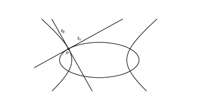
Figure 5. With Corollary 4.1 for $k=2$: The ellipse and hyperbola from the confocal pencil passing though $P$. The tangent $t_{1}$ to the ellipse at $P$ is the worst fit among all the lines containing $P$, while $t_{2}$, the tangent to the hyperbola at $P$ is the best fit among all such lines. The tangents $t_{1},t_{2}$ solve RPCA restricted at the point $P$.

We now formulate low-dimensional specializations of the last Theorem 4.3.

Corollary 4.1.

Let the system of points $M_{1},...,M_{N}$ with masses $m_{1},...,m_{N}$ be given in $\mathbb{R}^{k}$ with the associated pencil of confocal quadrics (3.4). Given a point $P$.

• For $k=2$ let the point $P$ have the Jacobi coordinates $(\lambda_{1}<\lambda_{2})$. The line which is the best fit for the given system of points among the lines which contain $P$ is the tangent line to the hyperbola with the parameter $\lambda=\lambda_{2}$. The line which is the worst fit for the given system of points among the lines which contain $P$ is the tangent line to the ellipse with the parameter $\lambda=\lambda_{1}$. The tangents $t_{1},t_{2}$ solve RPCA restricted at the point $P$. (See Fig. 5.)

• For $k=3$ let the point $P$ have the Jacobi coordinates $(\lambda_{1}<\lambda_{2}<\lambda_{3})$. The plane which is the best fit for the given system of points among the planes which contain $P$ is the tangent plane to the two-sheeted hyperboloid with the parameter $\lambda=\lambda_{3}$. The plane which is the worst fit for the given system of points among the planes which contain $P$ is the tangent plane to the ellipsoid with the parameter $\lambda=\lambda_{1}$. The lines of intersection of each two of the three tangent planes solve RPCA restricted at the point $P$.

Example 4.1.

Let $N$ points with masses $m_{1},...,m_{N}$ be given in the plane. Let us also fix a point $P$ in the plane. We will give the explicit formulas for the lines that are the best and the worst fit for the given system of $N$ points among the lines that contain the given point $P$, using the confocal pencil of conics (3.4) associated to the given system of $N$ points. Let $C$ be the centroid of the system of $N$ points. On our way, we provide the solution to the Restricted PCA at the point $P$, see (4.8).

Denote $Cxy$ the principal coordinate system of the confocal pencil and $J_{1}$ and $J_{2}$ as before, denote the principal planar moments of the inertia such that $J_{1}+ma_{2}^{2}=J_{2}.$ The confocal pencil of conics has the form

(4.6) $$\frac{x^{2}}{\alpha-\lambda}+\frac{y^{2}}{\beta-\lambda}=1,\quad\alpha=\frac{J_{1}}{m},\quad\beta=\frac{J_{1}}{m}-a_{2}^{2}.$$

For the point $P(x_{P},y_{P})$, its Jacobi elliptic coordinates $\lambda_{1}<\lambda_{2}$ are the solutions of the quadratic equation

(4.7) $$\lambda^{2}-(\alpha+\beta-x_{P}^{2}-y_{P}^{2})\lambda+\alpha\beta-\beta x_{P}^{2}-\alpha y_{P}^{2}=0.$$

The formula (4.5) gives the connection of the extremal values $J_{P_{1}}$ and $J_{P_{2}}$ of the principal planar inertia operator at the point $P$ with the Jacobi elliptic coordinates $\lambda_{1}$ and $\lambda_{2}$ of the point $P$, associated with the pencil of confocal conics: $J_{P_{1}}=2J_{1}-m\lambda_{2},\quad J_{P_{2}}=2J_{1}-m\lambda_{1}.$ We have already mentioned that the line that is the best fit among the lines that contain the point $P$ is the tangent to the $\lambda_{2}$-coordinate line through $P$, which is a hyperbola. The line that is the worst fit among those that contain $P$ is the tangent to the $\lambda_{1}$-coordinate line though $P$, and this is an ellipse. In order to find the equations of these lines of the best and wort fit, let us write the coordinate transformation between the Cartesian coordinates and the Jacobi elliptic coordinates (see [4, 15])

$$x^{2}=\frac{(\alpha-\lambda_{1})(\alpha-\lambda_{2})}{\alpha-\beta},\quad y^{2}=\frac{(\beta-\lambda_{1})(\beta-\lambda_{2})}{\beta-\alpha}.$$

Having in mind that the basal coordinate vectors are $\tilde{\mathbf{n}}_{(i)}=\Big{(}\frac{\partial x}{\partial\lambda_{i}},\frac{\partial y}{\partial\lambda_{i}}\Big{)}$ for $i=1,2$ one gets

(4.8) $$\tilde{\mathbf{n}}_{(1)}=-\frac{1}{2}\Big{(}\frac{\alpha-\lambda_{2}}{x_{P}(\alpha-\beta)}\ ,\frac{\beta-\lambda_{2}}{y_{P}(\beta-\alpha)}\Big{)},\quad\tilde{\mathbf{n}}_{(2)}=-\frac{1}{2}\Big{(}\frac{\alpha-\lambda_{1}}{x_{P}(\alpha-\beta)}\ ,\frac{\beta-\lambda_{1}}{y_{P}(\beta-\alpha)}\Big{)},$$

where it is supposed that $\lambda_{1}$ and $\lambda_{2}$ are functions of $x_{P}$ and $y_{P}$ obtained from (4.7). The pair $(\tilde{\mathbf{n}}_{(1)},\tilde{\mathbf{n}}_{(2)})$ from (4.8) is the solution of the Restricted PCA at the point $P$.

One finally gets the equations of the line that is the best fit:

(4.9) $$\frac{\alpha-\lambda_{2}}{x_{P}}(x-x_{P})-\frac{\beta-\lambda_{2}}{y_{P}}(y-y_{P})=0.$$

The equations of the line that is the worst fit is obtained analogously:

(4.10) $$\frac{\alpha-\lambda_{1}}{x_{P}}(x-x_{P})-\frac{\beta-\lambda_{1}}{y_{P}}(y-y_{P})=0.$$

Example 4.2.

Two types of cells in a fraction of the spleens, see [20], [19], [9], [8]. The data in this example are the numbers of two types of cells in a specified fraction of the spleens of fetal mice. They are displayed in Table 1. On the basis of sampling, it is reasonable to assume the original counts to be Poisson random variables, as explained in [9]. Therefore, the square roots of the counts are given in the last two columns of the table and they have, approximately, constant variance equal to $T^{-1}=1/4$. The postulated model is $y_{t}=\beta_{0}+\beta_{1}x_{t},$ where $(Y_{t},X_{t})=(y_{t},x_{t})+(e_{t},u_{t})$. Here $Y_{t}$ is the square root of the number of cells forming rosettes for the $t$-th individual, and $X_{t}$ is the square root of the number of nucleated cells for the $t$-th individual. On the basis of the sampling, the the pair of errors $(e_{t},u_{t})$ have a covariance matrix that is, approximately, $\Sigma=T^{-1}E=\operatorname{diag}(0.25,0.25)$, with $T=4$. The square roots of the counts cannot be exactly normally distributed, but we assume the distribution is close enough to normal to permit the use of the formulas based on normality. Thus, here we assume $\eta=1$.

Table 1. Numbers of two types of cells; following Cohen and D’Eustachio (1978), see [20]

j	$m_{j}$	$n_{j}$	$Y_{j}$	$X_{j}$
1	52	337	7.211	18.358
2	6	141	2.449	11.874
3	14	177	3.742	13.304
4	5	116	2.236	10.770
5	5	88	2.236	9.381

The coordinates of the centroid $C$ are $(\bar{x},\bar{y})=(12.7374,3.5748)$. One calculates that the components of the hyperplanar inertia operator $J_{C}$ at the centroid $C$ is: $J_{XX}=47.7937,J_{YY}=18.1021,J_{XY}=28.6318$. The principal hyperplanar moments of inertia $J_{1},J_{2}$ are the eigenvalues of the operator $J_{C}$. The corresponding eigenvectors are directions of the principal axes. The eigenvalues are $J_{1}=0.69605,J_{2}=65.19978$. The corresponding eigenvectors are $\mathbf{n}_{1}=(-0.51947,0.85449)^{T}$, $\mathbf{n}_{2}=(-0.85449,-0.51947)^{T}$. The equation of the line that best fits $u_{C}$ contains the centroid $C$ and is given by $u_{C}:y=0.60793x-4.16865.$ This coincides with the equations obtained in [20]. The equation of the line of the worst fit is $y=-1.64493x+24.52689.$

In the original study a hypothesis of interest is that $\beta_{0}=0$. This corresponds to the condition the line of regression contains the origin of coordinate system. Thus we will consider the origin of coordinate system, denoted by $(X,Y)$, as a point $P$. We want to apply Theorem 4.3 for a given point $P$. We introduce $(\tilde{X},\tilde{Y})$ as the principal coordinates having the centroid $C$ as the origin. Using a coordinate transformation, we recalculate the coordinates of the point $P$ in the principal coordinates and get: $(\tilde{X}_{P},\tilde{Y}_{P})=(3.56202,12.74098)$. Using (4.6), we get the pencil of conics associated with this data: it is defined with $\alpha=0.13921$, $\beta=-12.76154$:

(4.11) $$\frac{\tilde{x}^{2}}{0.13921-\lambda}+\frac{\tilde{y}^{2}}{-12.76154-\lambda}=1.$$

The Jacobi elliptic coordinates of the centroid $C$ are: $\lambda_{1_{C}}=\beta=-12.76154$, $\lambda_{2_{C}}=\alpha=0.13921.$From $J_{1}=2J_{1}-m\lambda_{2_{C}},$ we get $J_{1}=m\lambda_{2_{C}}=m\alpha.$Thus the moment of the line $u_{C}$ is equal to $m\lambda_{2_{C}}=J_{1}=0.69605$.

In order to find the Jacobi elliptic coordinates of the point $P$, associated to the pencil of conics (4.11), one needs to solve the quadratic equation (4.7). We get $\lambda_{1_{P}}=-186.907$ and $\lambda_{2_{P}}=-0.73589$ and as the Jacobi elliptic coordinates of the point $P$. Finally, the principal moments of inertia at the point $P$ are $J_{1_{P}}=2J_{1}-m\lambda_{2_{P}}=5.071564,\quad J_{2_{P}}=2J_{1}-m\lambda_{1_{P}}=935.9271.$ Using formulae (4.10) and (4.9) one gets that the equation of the line $u_{P}$ that is the best fit among the lines that contain $P$ is $u_{P}:\tilde{Y}=3.841884\tilde{X}-0.94389.$ In the original coordinates the equation of this line has the form $y=0.30014x.$ Thus, $\hat{\beta}_{1}=0.30014.$This quantity can be calculated also using [20], the equation at the bottom of p. 43, with $M_{xx}=171.8001$, $M_{xy}=51.26003$, $\hat{\lambda}=4.057252$, $\sigma_{uu}=0.25$, reads as $\hat{\beta}_{1}=(M_{xx}-\hat{\lambda}\sigma_{uu})^{-1}M_{xy}=0.30014.$

The line of best fit $u_{P}$ is tangent to the hyperbola from the confocal pencil of conics (4.11) which contains $P$:

$$\frac{\tilde{X}^{2}}{0.8751}+\frac{\tilde{Y}^{2}}{-12.0256}=1.$$

The moment of the line $u_{P}$ is $m(2\lambda_{2_{C}}-\lambda_{2_{P}})=J_{1_{P}}=5.071564$, with $m=5$.

The line of the worst fit among the lines that contain $P$ is $\tilde{Y}=-0.26029\tilde{X}+13.66814.$ In the original coordinates the equation of this line has the form $y=-3.331376x.$ It is tangent to the ellipse from the confocal family of conics (4.11) that contains $P$:

$$\frac{\tilde{X}^{2}}{187.0462}+\frac{\tilde{Y}^{2}}{174.1455}=1.$$

Figure 6. Example 4.2: The lines of the best and the worst fit tangent to the hyperbola and ellipse respectively, the confocal conics through the point $P$, the origin.

See Fig. 6. The bold point is the center of masses $C$. The two conics from the confocal pencil which pass through the point $P$, the origin, are presented. The line of the restricted orthogonal regression through the point $P$ is tangent to the hyperbola, while the line of the worst fit through the point $P$ is tangent to the ellipse.

For testing the null hypothesis $\beta_{0}=0$, the test statistic is [20] $N\hat{\lambda}/(N-1),$ whose null distribution can be approximated by Snedecor’s F distribution with degrees of freedom $(N-1)$ and $\infty$. Here, as in [20], $\hat{\lambda}$ is the smallest root of the equation $\det(J_{P}-\lambda\Sigma)=0$, where, as above $\Sigma=T^{-1}E=\operatorname{diag}(0.25,0.25)$, with $T=4$.

This statistic can be expressed as $5\hat{\lambda}/4=J_{1_{P}}=5(2\lambda_{2_{C}}-\lambda_{2_{P}}),$ See Theorem 4.4 for a more general statement. For these data, the value of $J_{1_{P}}$ is 5.071564. Therefore, the approximate p-value is $P(F_{4,\infty}>5.07)=0.00043$, which leads to rejection of the null hypothesis.

Remark 4.1.

The models with errors in variables for $\eta$ general were first studied by C.H. Kummell in 1879, see [20]. Now we want to treat the general cases of models with errors in variables in arbitrary dimension and with a nontrivial error covariance matrix, here denoted as $G$. We assume $G$ is known and positive definite. As it is well known, see e.g. [20], in such cases, the orthogonal regression should be performed not with respect to the ordinary Euclidean metric, but with respect to the metric generated by $G$. Thus, we consider a more general case when the inertia operator is defined with respect to the metric $\langle\cdot,\cdot\rangle_{G}=\langle G\cdot,\cdot\rangle$, where $\langle\cdot,\cdot\rangle$ is the Euclidean metric and $G$ is a positive definite matrix. The inertia operator is defined by

(4.12) $$(J^{G}_{O}\mathbf{n}_{G},\mathbf{m}_{G}) =\sum_{i=1}^{N}m_{i}\langle\mathbf{r}_{i},\mathbf{n}_{G}\rangle_{G}\langle\mathbf{r}_{i},\mathbf{m}_{G}\rangle_{G}$$

$$=\sum_{i=1}^{N}m_{i}\langle\sqrt{G}\mathbf{r}_{i},\sqrt{G}\mathbf{n}_{G}\rangle\langle\sqrt{G}\mathbf{r}_{i},\sqrt{G}\mathbf{m}_{G}\rangle.$$

We suppose that $\mathbf{n}_{G}$ is a unit vector in the metric defined with $G$. Let us introduce $\mathbf{n}=\sqrt{G}\mathbf{n}_{G}$, $\mathbf{m}=\sqrt{G}\mathbf{m}_{G}$. Then, $\mathbf{n}$ is a unit vector in the standard Euclidean metric $1=\langle G\mathbf{n}_{G},\mathbf{n}_{G}\rangle=\langle\sqrt{G}\mathbf{n}_{G},\sqrt{G}\mathbf{n}_{G}\rangle=\langle\mathbf{n},\mathbf{n}\rangle.$ Thus, we introduce new coordinates: $\mathbf{R}_{i}=\sqrt{G}\mathbf{r}_{i}.$We get $(J^{G}_{O}\mathbf{n}_{G},\mathbf{m}_{G})=(J_{O}\mathbf{n},\mathbf{m}),$ where $J_{O}$ is the inertia operator in the standard Euclidean metric in the new coordinates.The last relation can be rewritten as

$$(J_{O}\mathbf{n},\mathbf{m})=(J^{G}_{O}\mathbf{n}_{G},\mathbf{m}_{G})=\langle J^{G}_{O}\sqrt{G^{-1}}\mathbf{n},\sqrt{G^{-1}}\mathbf{m}\rangle=\langle\sqrt{G^{-1}}J^{G}_{O}\sqrt{G^{-1}}\mathbf{n},\mathbf{m}\rangle.$$

Thus, we conclude that $J_{O}=\sqrt{G^{-1}}J^{G}_{O}\sqrt{G^{-1}}.$Also, if $\mathbf{n}_{G}$ is an eigen-vector of the operator $J_{O}^{G}$, then $\mathbf{n}=\sqrt{G}\mathbf{n}_{G}$ is an eigen-vector of the operator $J_{O}$. The eigenvalue problem (4.2) in the metric $G$ case can be expressed as

(4.13) $$\det({J_{O}^{G}-\mu G})=\det(\sqrt{G^{-1}}J_{O}^{G}\sqrt{G^{-1}}-\mu E)=\det(J_{O}-\mu E)=0.$$

Theorem 4.4.

Let the system of $N$ points $M_{1},...,M_{N}$ with unit masses be given in $\mathbb{R}^{k}$, $N\geq k$, with the centroid $C$ and the associated pencil of confocal quadrics (3.4). For any point $P(x_{01},...,x_{0k})$ denote its Jacobi coordinates of the pencil of confocal quadrics (3.4) by $(\lambda_{1_{P}}<\dots<\lambda_{k_{P}})$ and the Jacobi coordinates of the centroid by $(\lambda_{1_{C}}<\dots<\lambda_{k_{C}})$. Then:

1. The hyperplanar moment of the hyperplane of the best fit is equal to $J_{1}=N\lambda_{k_{C}}$.

2. The hyperplanar moment of the hyperplane of the best fit that contains the point $P$ is equal to $J_{P}=N(2\lambda_{k_{C}}-\lambda_{k_{P}})$.

3. The test statistic of the hypothesis that the hyperplane of the best fit contains the point $P$ is:

   (4.14) $$\frac{N}{N-k+1}(2\lambda_{k_{C}}-\lambda_{k_{P}}).$$

   whose null distribution can be approximated by Snedecor’s F distribution with degrees of freedom $(N-k+1)$ and $\infty$.

5. The directional regressions and ellipsoids

In the previous sections we dealt primarily with geometric aspects of orthogonal regression. From the work of Galton [21] we know that conics play significant role in simple linear regression. From Fig. 1 one observes that points of horizontal and vertical tangency to the Galton ellipse (akka the ellipse of concentration) determine the lines of linear regression of $x$ on $y$ and of $y$ on $x$ respectively. This motivates our further study of linear regression in $\mathbb{R}^{k}$ in a geometric, invariant, i.e. coordinate free way. We consider linear regression in an arbitrary selected direction, not necessarily horizontal or vertical. In Section 5.1 we deal with the planar case and generalize this to an arbitrary $k$ in Section 5.2. A higher-dimensional geometric generalization of the above observation about Galton ellipses is given in Theorem 5.3, see also Corollary 5.3. The family of confocal quadrics (3.4) which we associated with the given system of points comes into picture here in reaching our third goal: for a given direction, for a given system of $N$ points, under the generality assumption, and for a selected point, find the best fitting hyperplane in the given direction. This is done in Theorem 5.4. The effectiveness of the developed methods and results and their applications in statistics are illustrated in Examples 5.1 and 5.2.

5.1. The directional axial moments in the plane

Given a line $w$ in the plane. Given $N$ points $M_{1},...,M_{N}$ with masses $m_{1},m_{2},...,m_{N}$ of the total mass $m$ in the plane. The point $C$ denotes the center of masses.

For a given line $u\subset\mathbb{R}^{2}$, non-parallel to $w$, the axial moment of inertia in direction $w$, denoted by $I^{w}_{u}$, is defined as

$$I^{w}_{u}=\sum\limits_{j=1}^{N}m_{j}\hat{d}_{j}^{2},$$

where $\hat{d}_{j}$ is the distance from the point $M_{j}$ to the point of intersection of the line $u$ with the line parallel to $w$ through the point $M_{j}$, $j=1,\dots,N$.

Suppose the line $u$ contains a point $O$. Denote by $\textbf{u}_{0}$ the unit vector parallel to the line $u$ and by $\textbf{w}_{0}$ the unit vector parallel to the line $w$. As before, we denote by $I_{u}$ the axial moment of inertia for the axis $u$ and by $I_{O}$ the operator of inertia for the point $O$. Then the axial moment of inertia $I^{w}_{u}$ for the axis $u$ in direction $w$ can be rewritten in the form:

(5.1) $$I^{w}_{u}=\sum\limits_{i=1}^{N}m_{i}\hat{d}_{i}^{2}=I_{u}\cdot\frac{1}{1-\langle\textbf{u}_{0},\textbf{w}_{0}\rangle^{2}}=\frac{\langle I_{O}\textbf{u}_{0},\textbf{u}_{0}\rangle}{1-\langle\textbf{u}_{0},\textbf{w}_{0}\rangle^{2}}.$$

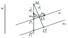
Figure 7. With formula (5.1) and with Proposition 5.1.

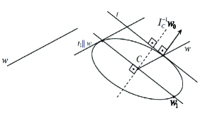
Figure 8. With Theorem 5.1.

From the last formula and Fig. 8, one easily gets, the following, directional version of the Huygens-Steiner Theorem:

Proposition 5.1.

[The directional Huygens-Steiner Theorem] Let the axis $u$ contain the center of masses $C$ and let $u_{1}$ be a line parallel to $u$. Denote by $I^{w}_{u_{1}}$ and $I^{w}_{u}$ the corresponding directional axial moments of inertia of a given system of points with the total mass $m$ in the direction $w$. Then

(5.2) $$I^{w}_{u_{1}}=I^{w}_{u}+m\hat{d}^{2},$$

where $\hat{d}$ is the distance between the points of intersection of a line parallel to $w$ with the parallel lines $u$ and $u_{1}$.

Thus, again we get a characterization of the center of masses, as a consequence of (5.2):

Corollary 5.1.

Given a direction $w$, the system of points and a direction $u$ not parallel to $w$. Among all the lines parallel to $u$, the least directional moment of inertia in direction $w$ is attained by the line through the center of masses of the system of points.

We will investigate the lines which minimize the directional axial moment in the direction $w$ and call them the directional lines of regression in the direction $w$. From the above Corollary we see that they have to pass through the center of masses $C$. Define the central axial ellipse of gyration as

(5.3) $$\langle I^{-1}_{C}\textbf{x},\textbf{x}\rangle=1.$$

Denote by $\hat{u}_{w}$ the direction of the directional line of regression in the direction $w$.

Theorem 5.1.

Let $w$ and $w_{1}$ form a pair of conjugate directions of the axial ellipse of gyration (5.3). Then the direction of the directional line of regression in the direction $w$ is orthogonal to $w_{1}$, i.e. $\langle\hat{u}_{w},w_{1}\rangle=0.$

Now we consider a similar problem, but searching for the best fit among the lines that contain a given point $P$, distinct from the center of masses: Find the line in the plane that contains a given point $P$ and has the minimal directional axial moment in the direction $w$.

Let $u$ and $u_{1}$ be two parallel lines, that contains $C$ and $P$ respectively. We assume that $u$ and $u_{1}$ are not parallel to $w$. Applying the Huygens-Steiner theorem (5.2), we get $I^{w}_{u_{1}}=I^{w}_{u}+m\hat{d}^{2}.$ Since $\hat{d}^{2}=\frac{{d}^{2}}{1-\langle u_{0},w_{0}\rangle^{2}}$ using (5.1), we get $I_{u_{1}}^{w}=\frac{I_{u}+m{d}^{2}}{1-\langle u_{0},w_{0}\rangle^{2}}=\frac{I_{u_{1}}}{1-\langle u_{0},w_{0}\rangle^{2}}=\frac{\langle I_{P}u_{0},u_{0}\rangle}{1-\langle u_{0},w_{0}\rangle^{2}}.$ The last formula is an analog of (5.1). Thus, we get:

Theorem 5.2.

Let $w$ and $w_{1}$ form a pair of conjugate directions of the axial ellipse of gyration $\langle I^{-1}_{P}x,x\rangle=1$ at a given point $P$. Then the direction of the directional line of regression in the direction $w$ at the point $P$ is orthogonal to $w_{1}$, i.e. $\langle\hat{u}_{w},w_{1}\rangle=0.$

5.2. The directional hyperplanar moments in $\mathbb{R}^{k}$

Let us select a line $w$ in $\mathbb{R}^{k}$. Given $N$ points $M_{1},...,M_{N}$ with masses $m_{1},m_{2},...,m_{N}$ of the total mass $m$ in $\mathbb{R}^{k}$. The point $C$ denotes the center of masses.

Now, we introduce the hyperplanar moment of inertia for the given system of points and for a given hyperplane $\pi\subset\mathbb{R}^{k}$, which is not parallel to $w$. We define $J^{w}_{\pi}$ the hyperplanar moment of inertia in direction $w$ as follows: $J^{w}_{\pi}=\sum\limits_{j=1}^{N}m_{j}\hat{D}_{j}^{2},$ where $\hat{D}_{j}$ is the distance between the point $M_{j}$ and the intersection of the hyperplane $\pi$ with the line parallel to $w$ through $M_{j}$, for $j=1,\dots,N$. Let n be the unit vector orthogonal to the hyperplane $\pi$, and $O$ a point contained in $\pi$. Then, using Fig. 10 the hyperplanar moment of inertia $J^{w}_{\pi}$ can be rewritten in the form

(5.4) $$J^{w}_{\pi}=\frac{J_{\pi}}{\langle\textbf{w}_{0},\textbf{n}\rangle^{2}}=\frac{\langle J_{O}\textbf{n},\textbf{n}\rangle}{\langle\textbf{w}_{0},\textbf{n}\rangle^{2}}.$$

Here $J_{\pi}$ is the hyperplanar moment of inertia and the operator $J_{O}$ is the hyperplanar inertia operator.

Proposition 5.2 (The hyperplanar directional Huygens-Steiner Theorem).

Let the hyperplane $\pi$ contain the center of masses $C$ and let $\pi_{1}$ be a hyperplane parallel to $\pi$. Denote by $J^{w}_{\pi_{1}}$ and $J^{w}_{\pi}$ the corresponding directional hyperplanar moments of inertia of a given system of points with the total mass $m$ in the direction $w$. Then

(5.5) $$J^{w}_{\pi_{1}}=J^{w}_{\pi}+m\hat{D}^{2},$$

where $\hat{D}$ is the distance between the points of intersection of a line parallel to $w$ with the parallel hyperplanes $\pi$ and $\pi_{1}$.

Thus, again we are getting a characterization of the center of masses, using (5.5):

Corollary 5.2.

Given a direction $w$, the system of points and one hyperplane $\pi$ not parallel to $w$. Among all the hyperplanes parallel to $\pi$, the least directional hyperplanar moment of inertia in direction $w$ is attained for the hyperplane which contains the center of masses of the system of points.

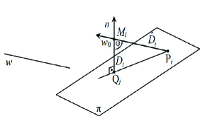
Figure 9. With equation (5.4).

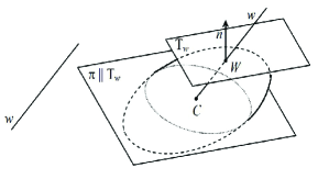
Figure 10. With Theorem 5.3.

We will investigate the hyperplanes which minimize the directional hyperplanar moment in the direction $w$ and call them the directional hyperplanes of regression in the direction $w$. From the above Corollary it follows that they contain the center of masses $C$. Define the ellipsoid of concentration as

(5.6) $$\langle J^{-1}_{C}\textbf{x},\textbf{x}\rangle=1.$$

Denote by $\hat{\pi}_{w}$ the directional hyperplane of regression in the direction $w$.

Theorem 5.3.

Let the radius vector from the center of masses $C$ in direction $w$ intersect the ellipsoid of concentration (5.6) at the point $W$ and let the tangent hyperplane to the ellipsoid of concentration at $W$ be $\pi_{W}$. The directional hyperplane of regression in the direction $w$ contains $C$ and is parallel to the tangent hyperplane $\pi_{W}$.

A statement similar to the last theorem can be extracted from [12], based on different considerations. For $k=2$ we get an important specialization of Theorem 5.3, see Fig. 12.

Corollary 5.3.

In the case $k=2$ the line of regression in the direction $w$ contains the center of masses $C$ and intersects the ellipse of concentration at two points at which the tangents to the ellipse of concentration are parallel to the line $w$. Equivalently, the line of regression is parallel to the tangent line of the ellipse of concentration at the point of its intersection with the iine parallel to $w$ passing through the centroid $C$.

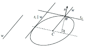
Figure 11. With Corollary 5.3.

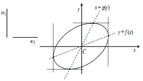
Figure 12. Simple linear regression.

For the proofs of the above theorems, see Section 6 of the Supplement [14] and for the examples, see in particular Examples 6.1 and 6.2 from there.

Now, as in the two-dimensional case, we consider the following problem for hyperplanes that contain a given point $P$ distinct from the center of masses: Find the hyperplane that contains a given point $P$ and has the minimal directional hyperplanar moment in the direction $w$.

Let $\pi$ and $\pi_{1}$ be two parallel hyperplanes that contain $C$ and $P$ respectively. We assume that $\pi$ and $\pi_{1}$ are not orthogonal to $w$. The Huygens-Steiner theorem (5.5) gives: $J^{w}_{\pi_{1}}=J^{w}_{\pi}+m\hat{D}^{2}.$ Since $\hat{D}^{2}=\frac{{D}^{2}}{\langle u_{0},w_{0}\rangle^{2}}$ using (5.4), we get $J_{\pi_{1}}^{w}=\frac{J_{\pi}+m{D}^{2}}{\langle u_{0},w_{0}\rangle^{2}}=\frac{J_{\pi_{1}}}{\langle u_{0},w_{0}\rangle^{2}}=\frac{\langle J_{P}u_{0},u_{0}\rangle}{\langle u_{0},w_{0}\rangle^{2}}.$ Here $J_{P}$ is given by (4.3). The last formula is an analog of (5.4). In statistics, the ellipsoid of concentration is typically considered at the centroid. In mechanics ellipsoids of inertia are not exclusively considered at the center of masses. Transporting this important flexibility from mechanics to statistics, we consider the ellipsoid of concentration at a given point. Let us recall that we described its principal hyperplanes in Theorem 4.2. Here the confocal pencil of quadrics (3.4) we constructed associated to the given system of points appears again. The principal hyperplanes are tangent hyperplanes at the point $P$ of those quadrics from the confocal pencil (3.4), which contain $P$. We get

Theorem 5.4.

Given the ellipsoid of concentration at a point $P$ $\mathcal{E}_{P}:\,\langle J^{-1}_{P}\textbf{x},\textbf{x}\rangle=1.$ Let the radius vector from the point $P$ in direction $w$ intersects the ellipsoid $\mathcal{E}_{P}$ at the point $W$. Let the tangent hyperplane to the ellipsoid $\mathcal{E}_{P}$ at $W$ be $\pi_{W}$. The directional hyperplane of regression in the direction $w$, among the hyperplanes which contain the point $P$, is parallel to the tangent hyperplane $\pi_{W}$.

Example 5.1.

Let $N$ points with masses $m_{1},...,m_{N}$ be given in the plane. Let us also fix a point $P$ in the plane. Among the lines that contain the given point $P$, we will derive formulas for the directional line of regression in the direction $w_{0}=(w_{x},w_{y})$ for the given system of points in the plane, using the associated confocal pencil of conics (3.4). We will provide the answer in terms of the Jacobi elliptic coordinates of the point $P$ with respect to the associated confocal pencil of conics.

We use the notation from Example 4.1. Denote by $C$ the centroid of the system of $N$ points. Denote $Cxy$ the principal coordinate system of the confocal pencil and $J_{1}$ and $J_{2}$ as before, denote the principal planar moments of the inertia. Introduce $a_{2}$ such that $J_{1}+ma_{2}^{2}=J_{2}.$ The confocal pencil of conics associated to the system of points (3.4) has the form

(5.7) $$\frac{x^{2}}{\alpha-\lambda}+\frac{y^{2}}{\beta-\lambda}=1,\quad\alpha=\frac{J_{1}}{m},\quad\beta=\frac{J_{1}}{m}-a_{2}^{2}.$$

We calculated the principal vectors $\tilde{\mathbf{n}}_{(1)}$ and $\tilde{\mathbf{n}}_{(2)}$ for the planar operator of inertia at the point $P$, see (4.8). In the corresponding orthogonal basis $[\mathbf{n}_{(1)},\mathbf{n}_{(2)}]$, the planar operator of inertia has a diagonal form $J_{P}=\operatorname{diag}(J_{P_{1}},J_{P_{2}}).$ The matrix of the change of bases $S$ is

$$S=\left(\begin{matrix}\frac{\alpha-\lambda_{2}}{\Delta_{1}x_{P}}&\frac{\alpha-\lambda_{1}}{\Delta_{2}x_{P}}\\ -\frac{\beta-\lambda_{2}}{\Delta_{1}y_{P}}&-\frac{\beta-\lambda_{1}}{\Delta_{2}y_{P}},\end{matrix}\right),\,\text{where}$$

$$\Delta_{1}=\sqrt{\frac{(\alpha-\beta)^{2}(\lambda_{2}-\lambda_{1})}{(\alpha-\lambda_{1})(\beta-\lambda_{1})}},\quad\Delta_{2}=\sqrt{\frac{(\alpha-\beta)^{2}(\lambda_{2}-\lambda_{1})}{(\alpha-\lambda_{2})(\lambda_{2}-\beta)}}.$$

In the new basis, the coordinates of the vector $w_{0}$ are

$$\tilde{w}_{1}=\frac{\alpha-\lambda_{2}}{\Delta_{1}x_{P}}w_{x}+\frac{\alpha-\lambda_{1}}{\Delta_{2}x_{P}}w_{y},\quad\tilde{w}_{2}=-\frac{\beta-\lambda_{2}}{\Delta_{1}y_{P}}w_{x}-\frac{\beta-\lambda_{1}}{\Delta_{2}y_{P}}w_{y}.$$

From Theorem 5.4 it follows that the regression line is parallel to $J_{P}^{-1}w_{0}$. Thus, the vector of the line of regression in the direction $w_{0}$ is $\mathbf{n}_{w}=S^{T}(\frac{\tilde{w}_{1}}{J_{P1}},\frac{\tilde{w}_{2}}{J_{P2}})^{T}.$ We get that $\mathbf{n}_{w}:=(n_{1},n_{2})^{T}$ is given by

$$n_{1} =\frac{1}{(\alpha-\beta)(\lambda_{2}-\lambda_{1})}\Big{[}\Big{(}\frac{(\alpha-\lambda_{2})(\beta-\lambda_{1})}{J_{P_{1}}}+\frac{(\alpha-\lambda_{1})(\lambda_{2}-\beta)}{J_{P_{2}}}\Big{)}w_{x}$$

$$+\sqrt{(\alpha-\lambda_{1})(\alpha-\lambda_{2})(\beta-\lambda_{1})(\lambda_{2}-\beta)}\Big{(}\frac{1}{J_{P_{1}}}-\frac{1}{J_{P_{2}}}\Big{)}w_{y}\Big{]}$$

$$n_{2} =\frac{1}{(\alpha-\beta)(\lambda_{2}-\lambda_{1})}\Big{[}\sqrt{(\alpha-\lambda_{1})(\alpha-\lambda_{2})(\beta-\lambda_{1})(\lambda_{2}-\beta)}\Big{(}\frac{1}{J_{P_{1}}}-\frac{1}{J_{P_{2}}}\Big{)}w_{x}$$

$$+\Big{(}\frac{(\alpha-\lambda_{1})(\lambda_{2}-\beta)}{J_{P_{1}}}+\frac{(\beta-\lambda_{1})(\alpha-\lambda_{2})}{J_{P_{2}}}\Big{)}w_{y}.$$

From Example 4.1 we know that the formula (4.5) gives the connection of the extremal values $J_{P_{1}}$ and $J_{P_{2}}$ of the principal planar inertia operator at the point $P$ with the Jacobi elliptic coordinates $\lambda_{1}$ and $\lambda_{2}$ of the point $P$, associated with the pencil of confocal conics: $J_{P_{1}}=2J_{1}-m\lambda_{1},\quad J_{P_{2}}=2J_{1}-m\lambda_{2}.$ The coordinate transformation between the Cartesian coordinates and the Jacobi elliptic coordinates also gives $x^{2}_{P}$ and $y^{2}_{P}$ in terms of the Jacobi elliptic coordinates $\lambda_{1}$ and $\lambda_{2}$ of the point $P$, associated with the confocal pencil (5.7):

$$x^{2}_{P}=\frac{(\alpha-\lambda_{1})(\alpha-\lambda_{2})}{\alpha-\beta},\quad y^{2}_{P}=\frac{(\beta-\lambda_{1})(\beta-\lambda_{2})}{\beta-\alpha}.$$

Thus we get the formula for the line of regression in the direction $w_{0}$ under the restriction that it contains a given point $P$ in terms of the Jacobi elliptic coordinates of the point $P$ with respect to the confocal pencil of conics (5.7) associated with the given system of points.

The line of the best fit passing through the point $P$ is $y-y_{P}=\kappa(x-x_{P}),\quad\kappa=-{n_{1}}/{n_{2}}.$

Example 5.2.

Predicting pressure from the boiling point of water. See [11], [17]. The results from experiments that were trying to obtain a method for estimating altitude were presented in [17]. A formula is available for altitude in terms of barometric pressure, but it was difficult to carry a barometer to high altitudes in the XIX century. However, it might be easy for travelers to carry a thermometer and measure the boiling point of water. Table 2 contains the measured barometric pressures and boiling points of water from $17$ experiments.

Table 2. 17 Forbes’ observations

j	1	2	3	4	5	6	7	8	9	10
$x_{j}$	194.5	194.3	197.9	198.4	199.4	199.9	200.9	201.1	201.4	201.3
$y_{j}$	20.79	20.79	22.40	22.67	23.15	23.35	23.89	23.99	24.02	24.01

j	11	12	13	14	15	16	17
$x_{j}$	203.6	204.6	209.5	208.6	210.7	211.9	212.2
$y_{j}$	25.14	26.57	28.49	27.76	29.04	29.88	30.06

One can use the method of least squares to fit a linear relationship between boiling point and pressure. Let $y_{i}$ be the pressure for one of Forbes’ observations, and let $x_{i}$ be the corresponding boiling point for $i=1,\dots,17$. Using the data in Table 2, we can compute the covariance matrix. The coordinates of the centroid are $(\bar{x},\bar{y})=(202.9529,25.05882)$. The components of the hyperplanar inertia operator at the centroid are $J_{xx}=530.78235,J_{yy}=145.93778,J_{xy}=277.54206$. The principal moments of inertia are $J_{1}=0.63839,J_{2}=676.08147$. Then we compute the line $u_{C}$ of the best fit as the least-squares line. The intercept and slope of the line $u_{C}$ are, respectively, $\hat{\beta}_{0}=-81.06373$ and $\hat{\beta}_{1}=0.5228$. Using formula (5.4), one calculates the directional moment of inertia $J^{w}_{u_{C}}=0.813143014$.

A traveler is interested in the barometric pressure when the boiling point of water is $201.5$ degrees. Suppose that this traveler would like to know whether the pressure is $24.5$. Thus, the traveler might wish to test the null hypothesis $H_{0}:\beta_{0}+201.5\beta_{1}=24.5$, versus $H_{1}:\beta_{0}+201.5\beta_{1}\neq 24.5$.

Figure 13. Example 5.1: The line of restricted regression and confocal quadrics through the point P.

Here we are now interested in the line of regression of $y$ on $x$, i.e. in the vertical direction, under the restriction that it contains the point $P(201.5,24.5)$. Now, we introduce $(\tilde{x},\tilde{y})$ as the principal coordinates at the centroid. Using the coordinate transformation from the original to the principal coordinates, we calculate the coordinates of the point $P$ in the principal system: $\tilde{x}_{P}=0.08698$, $\tilde{y}_{P}=-1.68554$. Similarly, the vertical vector $(0,1)$ in the new coordinate system becomes ${\mathbf{w}}_{0}=(-0.88594,0.46381)$. Our pencil of conics associated to the data is defined with $\alpha=0.037552$, $\beta=-39.69441$:

$$\frac{\tilde{x}^{2}}{0.037552-\lambda}+\frac{\tilde{y}^{2}}{-39.69441-\lambda}=1.$$

The Jacobi elliptic coordinates of the point $P$ are the solutions of the quadratic equation (4.7): $\lambda_{1P}=-42.536$, $\lambda_{2P}=0.03049$,. The principal hyperplanar moments of inertia at the point $P$ are $J_{1_{P}}=2J_{1}-m\lambda_{2_{P}}=0.75841\quad J_{2_{P}}=2J_{1}-m\lambda_{1_{P}}=724.3882$ In the principal coordinates $\mathbf{n}_{w}=\tilde{S}^{T}(\frac{\tilde{w}_{1}}{J_{P_{1}}},\frac{\tilde{w}_{2}}{J_{P_{2}}})^{T}$.

The equation of the line of the best fit in the sense of least squares passing through the point $P$ is $u_{P}:\tilde{\tilde{y}}=1189.499993\tilde{\tilde{x}}-211.1392.$ Using formula (5.4), we calculate the corresponding directional moment of inertia $J^{w}_{u_{P}}=1.455877$. In the original coordinates, the equation of the line of the best fit $u_{P}$ is $y=0.5141352x-79.0982450.$

The F-statistic $F=\frac{RSS_{1}-RSS_{2}}{p_{2}-p_{1}}/\frac{RSS_{2}}{N-p_{2}},$ for $N=17$, $p_{2}=2$, $p_{1}=1$ is 11.85647, while p-value is $P(F_{1,15}>11.85647)=0.003621119.$ The null hypothesis should be rejected, leading to the conclusion that pressure is not 24.5 (see Fig. 13).

Remark 5.1.

Our calculations from this example do not coincide with the calculations from [11]. For example, for unconstrained problem they got $\hat{\beta}_{0}=-81.049$ while the correct value is $\hat{\beta}_{0}=-81.06373$, as above.

It is interesting to note that in [5], following [29], they discuss this experiment from the point of view of errors in measurement models.

6. Acknowledgements

We are grateful to Maxim Arnold for indicating the reference [22] and for interesting discussions. We are also grateful to Pankaj Choudhary, Sam Efromovich, and Frank Konietschke for interesting discussions. This research has been partially supported by Mathematical Institute of the Serbian Academy of Sciences and Arts, the Science Fund of Serbia grant Integrability and Extremal Problems in Mechanics, Geometry and Combinatorics, MEGIC, Grant No. 7744592 and the Ministry for Education, Science, and Technological Development of Serbia and the Simons Foundation grant no. 854861.

References

- [1] Adcock, R. J. (1877). Note on the method of least squares. Analyst 4, 183–184.
- [2] Adcock. R. J. (1878). A problem in least squares. Analyst, 5, 53–54.
- [3] Andreson, T. W. (1958). An Introduction to Multivariate Statistical Analysis John Wiley and Sons.
- [4] Arnold, V. I. (1989). Mathematical methods of classical mechanics, Graduate Texts in Mathematics, 60, 2nd edition, Springer-Verlag, New York, pp. xvi+508
- [5] Carroll, R. J., Ruppert, D. (1996). The use and misuse of orthogonal regression estimation in linear errors-in-variables models. The American Statistician, 50, 1–6.
- [6] Carroll, R., Ruppert, D., Stefanski L., Crainiceanu, C. (2006). Measurement Error in Nonlinear Models, A Modern Perspective Second Edition, Monographs on Statistics and Applied Probability 105, Taylor and Francis.
- [7] Casella G., Berger, R. L. (2001). Statistical Inference, Second Edition, Duxbury Advanced Series, Duxbury.
- [8] Cohen, J. E., D’Eustachio, P. and Edelman, G. M. (1977). The specific antigenbinding cell populations of individual fetal mouse spleens: Repertoire composition, size and genetic control. J. Exp. Med., 146, 394–411.
- [9] Cohen, J. E. and D’Eustachio, P. (1978). An affine linear model for the relation between two sets of frequency counts. Response to a query, Biometrics 34,514–516.
- [10] Cramér, H. (1946). Mathematical Methods of Statistics, Princeton: Princeton University Press.
- [11] DeGroot, M., Schervish, M. (2012). Probability and Statistics, Fourth Edition, Adison-Wesley.
- [12] Dempster, A. (1969). Elements of continuous multivariate analysis, Addison-Wesley.
- [13] Dragović, V. Gajić, B. (2022) Points with symmetric ellipsoids of inertia and envelopes of, hyperplanes which equally fit the system of points in , submitted
- [14] Dragović, V. Gajić, B. (2022). Supplement to “Orthogonal and Linear Regressions and Pencils of Confocal Quadrics”.
- [15] Dragović, V. Radnović, M. (2011). Poncelet Porisms and Beyond: Integrable Billiards, Hyperelliptic Jacobians and Pencils of Quadrics, Frontiers in Mathematics, Basel: Springer.
- [16] T. B. Fomby, R. C. Hill, S. R. Johnson (1984). Advanced Econometric Methods, Springer Science + Business Media.
- [17] Forbes, J. D. (1857). Further experiments and remarks on the measurement of heights by the boiling point of water, Transactions of the Royal Society of Edinburgh, 21: 135-143.
- [18] Friendly, M., Monette, G., Fox, J. (2013). Elliptic insights: understanding statistical methods through elliptical geometry. Statist. Sci. 28, no. 1, 1–39.
- [19] Fuller, W. A. (1978). An affine linear model for the relation between two sets of frequency counts: Response to query. Biometrics 34, 517–521.
- [20] Fuller, W. A. (1987). Measurement Error Models, John Willey and Sons.
- [21] Galton, F. (1886). Regression towards mediocrity in hereditary stature. Journal of the Anthropological Institute, 15, pp. 246–263.
- [22] Gardiner, M. (1893). On ”Confocal Quadrics of Moments of Inertia” pertaining to all Planes in Space, and Loci and Envelopes of Straight Lines whose ”Moments of Inertia” are Constants, Proceedings of the Royal Society of Victoria, 5, 200–208.
- [23] Goodfellow, I., Bengio, Y., Courville, A. (2016). Deep learning The MIT Press.
- [24] Hastie, T., Tibshirani, R., Friedman, J (1977) The elements of statistical learning Second Edition, Springer
- [25] Pearson, K. (1901). On Lines and Planes of Closest Fit to Systems of Points in Space, Phil. Mag. 2, 559–572.
- [26] Rogers, A. J. (2013). Concentration Ellipsoids, Their Planes of Support, and the Linear Regression Model, Econometric Reviews, 32:2, 220-243, DOI:10.1080/07474938.2011.608055.
- [27] Seber, G., Lee, A. (2003) Linear Regression Analysis Second Edition, John Wiley and Sons.
- [28] Suslov, G.K. (1900) Fundamentals of Anaytical Mechanics, Vol.1, Kiev, [in Russian].
- [29] Weisberg, S. (1985) Applied Linear Regression, Second Edition, John Willey and Sons.