Conjugate Modeling Approaches for Small Area Estimation with Heteroscedastic Structure

Paul A. Parker, Scott H. Holan¹, and Ryan Janicki¹

Abstract

Small area estimation has become an important tool in official statistics, used to construct estimates of population quantities for domains with small sample sizes. Typical area-level models function as a type of heteroscedastic regression, where the variance for each domain is assumed to be known and plugged in following a design-based estimate. Recent work has considered hierarchical models for the variance, where the design-based estimates are used as an additional data point to model the latent true variance in each domain. These hierarchical models may incorporate covariate information, but can be difficult to sample from in high-dimensional settings. Utilizing recent distribution theory, we explore a class of Bayesian hierarchical models for small area estimation that smooth both the design-based estimate of the mean and the variance. In addition, we develop a class of unit-level models for heteroscedastic Gaussian response data. Importantly, we incorporate both covariate information as well as spatial dependence, while retaining a conjugate model structure that allows for efficient sampling. We illustrate our methodology through an empirical simulation study as well as an application using data from the American Community Survey.

Keywords: Gibbs sampling, ICAR, Mixed Models, Multivariate log-Gamma, Spatial.

1 Introduction

Population estimates for small areas or domains, defined as geographic regions or demographic subpopulations, based on survey data have garnered high demand in recent years. These direct estimates, which use only domain-specific survey response data, may not be sufficiently precise for reliable inference due to small sample sizes and unreasonably high standard errors. To meet this demand, model based approaches, or small area estimation (SAE) models, are commonly used in place of direct estimates. Area-level models such as the popular Fay-Herriot (FH) model (Fay III and Herriot,, 1979) can incorporate covariates or other dependencies in order to smooth the direct estimates and improve precision by “borrowing strength” from areas with large sample size. The FH model assumes that the sample variance of the direct estimator is fixed and known, which is rarely the case in real survey data settings. In practice, the sampling variance is estimated from the survey data and then plugged into the model. Sampling variances tend to vary across geographic areas, thus, these area-level SAE models may be seen as a type of model for heteroscedastic data.

Recently, a variety of extensions to the FH model have been considered in order to address the issue of unknown sampling variances (You and Chapman,, 2006; You,, 2021). For example, Maiti et al., (2014) use a hierarchical modeling approach to jointly smooth both direct mean and variance estimates. Sugasawa et al., (2017) fit a similar model in a Bayesian setting. In both cases, covariates may be used to aid in the variance smoothing, but in the Bayesian case, Sugasawa et al., (2017) required the use of a Metropolis-Hastings step within the Gibbs sampler, due to a full-conditional distribution with unknown form.

Incorporating estimates of the sampling error variance of the direct estimator is a topic of significant interest in the course of producing model-based estimates for official statistics. In this direction, Bradley et al., (2016) propose a model to include both the direct estimates and an estimate of the sampling error variance in a Poisson area-level spatial change-of-support model for the American Community Survey (ACS). The proposed model uses the variance estimates as another data source and exploits the Poisson equidispersion assumption (i.e., equal mean and variance) to condition on a common latent process.

The approach proposed here differs from Bradley et al., (2016) and exploits the distribution theory of Bradley et al., (2020). Specifically, we extend the approach proposed in Parker et al., (2021) for heteroscedastic data to the SAE setting for both area-level and unit-level models. Importantly, our approach yields models that are fully conjugate for both the mean and variance regression parameters, and thus leads to extremely computationally efficient estimation (see Sections 2 and 3 for additional detail).

Although SAE methods have a long and rich history, the literature on jointly modeling the mean (direct estimates) and variance (sampling error variance) is significantly more recent by comparison. For example, Savitsky and Gershunskaya, (2022) propose a Bayesian nonparametric model that jointly models the mean and the variance in the context of the Consumer Expenditure Survey (CES). Similarly, Polettini, (2017) proposes a semiparametric Bayesian Fay-Herriot model that shrinks both the means and variance. In general, these approaches can be computationally expensive and, thus, there is a need for models that scale computationally to meet the high-dimensional demands that are faced by statistical agencies and subject-matter practitioners. The method proposed here meets this demand.

Outside of the SAE literature there exists a substantial literature on joint models for the mean and covariance. For example, Pourahmadi, (1999, 2011) and Chen and Dunson, (2003), among others, model Cholesky-based factorizations of unstructured covariances. In general these methods are extremely useful; nevertheless, they are not immediately applicable to the SAE problems considered here. In particular, the SAE setting is comprised of a diagonal covariance (variance) structure with a model on the latent variances. A comprehensive review of Cholesky-based joint mean and covariance modeling can be found in Pourahmadi, (2013) and the references therein.

There has also been significant research on modeling covariance structure using covariates, many of which arise in the spatio-temporal literature. For example, see Schmidt et al., (2011) and Gladish et al., (2014), among others. The main challenge that arises in this context is computational. In general, most of the proposed methods proceed using Bayesian methods and lead to non-conjugate updates, necessitating migration away from straightforward Gibbs sampling. One notable exception is proposed by Parker et al., (2021), which provides a starting point for the method proposed here.

This paper also proposes a novel unit-level SAE model for heteroscedastic Gaussian survey data. The main complication of unit-level SAE modeling is accounting for the survey design in the model. When the survey design is noninformative, in the sense that the distribution of the sampled response values is the same as the distribution of the unsampled values, the effect of the survey design can largely be ignored. However, when the probability of selection in the survey is correlated with the response variable, the survey design is said to be informative, in which case the population distribution and the distribution for the sampled data will differ. Under informative sampling, the survey design must be carefully accounted for in the SAE model to avoid biased estimates. To this end, we also propose a heteroscedastic unit-level model under informative sampling using the pseudo-likelihood (Binder,, 1983; Skinner,, 1989; Savitsky and Toth,, 2016). For a comprehensive review of unit-level approaches to SAE see Parker et al., (2019) and the references therein.

Although the methodology proposed here is extremely general and applies to a broad set of applications that are encountered by data users and official statistical agencies, our motivating example considers income estimation and is related to the Small Area Income and Poverty Estimates Program (SAIPE). In particular, SAIPE produces income estimates for all U.S. states and counties (Bell et al.,, 2016) and in many cases, the estimates may be used in the administration of federal programs and the allocation of federal funds to local jurisdictions.. Therefore, using the American Community Survey (ACS) we demonstrate our proposed approach by estimating the average income by PUMA for the state of California.

This paper proceeds as follows. Section 2 provides background and introduces our heteroscedastic model for area-level data. Unit-level models are presented in Section 3. To evaluate the effectiveness of our approach, an empirical simulation study is provided in Section 4 and an analysis of ACS income data is presented in Section 5. Discussion is provided in Section 6.

2 Area-level Heteroscedastic Models

2.1 Background

The FH model (Fay III and Herriot,, 1979) is given by

$$y_{i}|\theta_{i},\sigma^{2}_{i} \stackrel{{\scriptstyle ind}}{{\sim}}\hbox{N}(\theta_{i},\sigma^{2}_{i}),\;i=1,\ldots,d$$

$$\theta_{i} =\bm{x}_{i}^{\prime}\bm{\beta}+\nu_{i}$$

$$\nu_{i} \stackrel{{\scriptstyle ind}}{{\sim}}\hbox{N}(0,\sigma^{2}_{\nu}),$$

where $y_{i}$ is the direct estimate, $\sigma^{2}_{i}$ is the sampling variance of the direct estimate and is assumed known, and $i=1,\dots,d$ indexes the small areas of interest. Thus, the FH model may be seen as a type of heteroscedastic data model where the variance is known. Typically, the true value of $\sigma^{2}_{i}$ is unknown, thus a design-based estimate, $s^{2}_{i}$ is plugged in instead.

In order to reflect the additional uncertainty attributed to $s_{i}^{2},$ a second data model may be used. For example, You and Chapman, (2006) suggest the following model to address the issue of unknown sample variances,

$$y_{i}|\theta_{i},\sigma^{2}_{i} \stackrel{{\scriptstyle ind}}{{\sim}}\hbox{N}(\theta_{i},\sigma^{2}_{i}),\;i=1,\ldots,d$$

$$s_{i}^{2}|\sigma_{i}^{2} \stackrel{{\scriptstyle ind}}{{\sim}}\hbox{Gamma}\left(\frac{n_{i}-1}{2},\frac{n_{i}-1}{2\sigma^{2}_{i}}\right),\;i=1,\ldots,d$$

$$\theta_{i} =\bm{x}_{i}^{\prime}\bm{\beta}+\nu_{i}$$

$$\nu_{i} \stackrel{{\scriptstyle ind}}{{\sim}}\hbox{N}(0,\sigma^{2}_{\nu})$$

$$\sigma^{2}_{i} \stackrel{{\scriptstyle ind}}{{\sim}}\hbox{IG}(a_{i},b_{i}),$$

where $n_{i}$ represents the sample size in area $i$ and $\hbox{IG}(a,b)$ denotes an inverse gamma distribution with shape parameter $a$ and scale parameter $b$. In principal, the data model for $s_{i}^{2}$ given here is only valid in the case of a simple random sample within area $i$. For complex sample designs, it may be important to give careful consideration to the degrees of freedom. Although estimation of the appropriate degrees of freedom is beyond the scope of this work, for more discussion on this matter, see Maples et al., (2009).

Sugasawa et al., (2017) provide a Bayesian extension of this approach that considers covariates in the variance model by letting $\sigma^{2}_{i}\stackrel{{\scriptstyle ind}}{{\sim}}\hbox{IG}\left(a_{i},b_{i}\hbox{exp}(\bm{x}_{2i}^{\prime}\bm{\beta}_{2})\right)$. Although the use of covariates here may improve small area estimates, Sugasawa et al., (2017) required the use of a Metropolis-Hastings sampler for $\bm{\beta}_{2}$, which can be extremely difficult to tune, especially in high dimensions.

2.2 Conjugate Priors for Heteroscedastic Models

The foundation of our modeling framework is the multivariate log-Gamma distribution (MLG), introduced by Bradley et al., (2018) and Bradley et al., (2020). The MLG distribution was initially developed in order to model dependent data using a Poisson likelihood. The density for the MLG distribution is given as

$$f(\bm{y})=\hbox{det}(\bm{V}^{-1})\left\{\prod_{i=1}^{n}\frac{\kappa_{i}^{\alpha_{i}}}{\Gamma(\alpha_{i})}\right\}\hbox{exp}\left[\bm{\alpha}^{\prime}\bm{V}^{-1}(\bm{y-\mu})-\bm{\kappa}^{\prime}\hbox{exp}\left\{\bm{V}^{-1}(\bm{y-\mu})\right\}\right],$$ (1)

denoted by $\hbox{MLG}(\bm{\mu},\mathbf{V},\bm{\alpha},\bm{\kappa})$. The length $n$ vector $\bm{\mu}$ acts as a centrality parameter and the $n\times n$ matrix $\bm{V}$ controls the correlation structure. The length $n$ vectors $\bm{\alpha}$ and $\bm{\kappa}$ are shape and rate parameters respectively. Sampling from $\bm{Y}\sim\hbox{MLG}(\bm{\mu},\mathbf{V},\bm{\alpha},\bm{\kappa})$ is straightforward using the following steps:

1. Generate a vector $\mathbf{g}$ as $n$ independent Gamma random variables with shape $\alpha_{i}$ and rate $\kappa_{i}$, for $i=1,\ldots,n$

2. Let $\mathbf{g}^{*}=\hbox{log}(\mathbf{g})$

3. Let $\mathbf{Y}=\mathbf{Vg}^{*}+\bm{\mu}$.

In most cases, Bayesian inference using the MLG prior distribution also requires simulation from the conditional multivariate log-Gamma distribution (cMLG). Letting $\mathbf{Y}\sim\hbox{MLG}(\bm{\mu},\mathbf{V},\bm{\alpha},\bm{\kappa})$, Bradley et al., (2018) show that $\mathbf{Y}$ can be partitioned into $(\mathbf{Y_{1}}^{\prime},\mathbf{Y_{2}}^{\prime})^{\prime}$, where $\mathbf{Y_{1}}$ is $r$-dimensional and $\mathbf{Y_{2}}$ is $(n-r)$-dimensional. The matrix $\mathbf{V}^{-1}$ is also partitioned into $\left[\mathbf{H\;B}\right]$, where $\mathbf{H}$ is an $n\times r$ matrix and $\mathbf{B}$ is an $n\times(n-r)$ matrix. Then

$$\bm{Y_{1}}|\bm{Y_{2}}=\bm{d},\bm{\mu}^{*},\bm{H},\bm{\alpha},\bm{\kappa}\sim\hbox{cMLG}(\bm{\mu}^{*},\bm{H},\bm{\alpha},\bm{\kappa})$$

with density

$$M\hbox{exp}\left\{\bm{\alpha}^{\prime}\bm{HY_{1}}-\bm{\kappa}^{\prime}\hbox{exp}(\bm{HY_{1}}-\bm{\mu}^{*})\right\}I\left\{(\bm{Y_{1}}^{\prime},\bm{d}^{\prime})^{\prime}\in\mathcal{M}^{n}\right\},$$ (2)

where $\bm{\mu}^{*}=\mathbf{V}^{-1}\bm{\mu}-\mathbf{Bd}$, and $\mathit{M}$ is a normalizing constant. Bradley et al., (2018) show that it is also straightforward to sample from the cMLG distribution using $(\mathbf{H}^{\prime}\mathbf{H})^{-1}\mathbf{H}^{\prime}\mathbf{Y}$, where $\mathbf{Y}$ is sampled from $\hbox{MLG}(\bm{\mu},\mathbf{I},\bm{\alpha},\bm{\kappa})$.

Another key result given by Bradley et al., (2018) is that $\hbox{MLG}(\mathbf{c},\alpha^{1/2}\mathbf{V},\alpha\mathbf{1},\alpha\mathbf{1})$ converges in distribution to a multivariate normal distribution with mean $\mathbf{c}$ and covariance matrix $\mathbf{VV^{\prime}}$ as the value of $\alpha$ approaches infinity. This allows for the computational benefits of MLG priors while maintaining effectively the same shape and structure as a Gaussian prior.

Although the original use of the MLG distribution was as a prior in high-dimensional Poisson regression, recently Parker et al., (2021) found that the MLG distribution acts as a conjugate prior for variance regression when using a negative log link function. This insight is the basis for our proposed approach.

2.3 Proposed Area-Level Approach

In order to account for the additional uncertainty around $s_{i}^{2}$ in the context of area-level SAE, we construct a joint model for the direct point estimate and variance. Critically, this model relies on the MLG distribution as a conjugate prior for the variance regression parameters. Our heteroscedastic area-level model (HALM) is given as

$${y_{i}}|\theta_{i},\sigma^{2}_{i} \stackrel{{\scriptstyle ind}}{{\sim}}\hbox{N}(\theta_{i},\sigma^{2}_{i}),\;i=1,\ldots,d$$

$${s_{i}^{2}}|\sigma_{i}^{2} \stackrel{{\scriptstyle ind}}{{\sim}}\hbox{Gamma}\left(\frac{{n_{i}}-1}{2},\frac{{n_{i}}-1}{2\sigma^{2}_{i}}\right),\;i=1,\ldots,d$$

$$\theta_{i} ={\bm{x}_{i}}^{\prime}\bm{\beta}_{1}+\eta_{1i}$$

$$-\hbox{log}(\sigma^{2}_{i}) ={\bm{x}_{i}}^{\prime}\bm{\beta}_{2}+\eta_{2i}$$

$$\bm{\eta}_{1}|\sigma^{2}_{\eta_{1}} \sim\hbox{N}(\bm{0},\sigma^{2}_{\eta_{1}}\bm{\hbox{I}})$$

$$\bm{\eta}_{2}|\sigma^{2}_{\eta 2} \sim\hbox{MLG}(\bm{0},\alpha^{1/2}\sigma_{\eta_{2}}\bm{\hbox{I}},\alpha\bm{1},\alpha\bm{1})$$

$$\bm{\beta}_{1} \sim\hbox{N}(\bm{0},\sigma^{2}_{\beta_{1}}\bm{\hbox{I}})$$

$$\bm{\beta}_{2} \sim\hbox{MLG}(\bm{0},\alpha^{1/2}\sigma_{\beta_{2}}\bm{\hbox{I}},\alpha\bm{1},\alpha\bm{1})$$

$$\sigma^{2}_{\eta_{1}} \sim\hbox{IG}(a,b)$$

$$\sigma_{\eta_{2}} \sim\hbox{N}^{+}(0,c).$$

Here, $y_{i}$ represents the direct estimate of an unknown population quantity, $\theta_{i},$ while $s_{i}^{2}$ represents the design-based variance around this estimate. The unknown population quantity is written as a linear combination of the length $p$ vector of covariates, $\bm{x}_{i},$ as well as an area level random effect, $\eta_{1i}.$ The unknown variance, $\sigma_{i}^{2},$ is modeled using the negative log link function as a linear combination of $\bm{x}_{i}$ as well as an additional area-level random effect, $\eta_{2i}.$ In order to establish conjugate full-conditional distributions, $\beta_{2}$ takes on a MLG prior distribution that is asymptotically equivalent to a $\hbox{N}(\bm{0},\sigma^{2}_{\beta}\bm{\hbox{I}})$ distribution. Similarly, conditional on $\sigma^{2}_{\eta_{2}},$ $\bm{\eta}_{2}$ takes a MLG prior distribution that is asymptotically equivalent to a $\hbox{N}(\bm{0},\sigma^{2}_{\eta_{2}}\bm{\hbox{I}})$ distribution. Finally, we place a conjugate inverse Gamma prior distribution on $\sigma^{2}_{\eta_{1}}$ as well as a half-normal prior on $\sigma_{\eta_{2}}.$ We note that this prior for $\sigma_{\eta_{2}}$ is not conjugate, and thus requires a Metropolis-Hastings step. However, this is only for a single parameter and we have found that there is very little effect on the mixing of the MCMC due to this. We use a random-walk Metropolis-Hastings step with a Normal distribution truncated below at zero for a proposal distribution, although, depending on the setting, it may be helpful to consider other proposals. The model is completed by specification of $\alpha,\sigma^{2}_{\beta_{1}},\sigma^{2}_{\beta_{2}},a,b,c>0.$ In practice, we work with relatively diffuse priors by using $\sigma^{2}_{\beta_{1}}=\sigma^{2}_{\beta_{2}}=1000,$ $a=b=0.5,$ and $c=5.$ The value for $\alpha$ should be sufficiently large to invoke the asymptotic equivalence to the multivariate normal distribution. Similar to Bradley et al., (2018), we have found $\alpha=1000$ to be sufficient for our purposes, although in some other cases this may be data dependent.

Often within SAE, more precise estimates can be generated through the use of spatial dependence modeling (e.g., see Marhuenda et al., (2013); Porter et al., (2015)). This motivates the need for spatially correlated prior structures for the mean and variance models. To this end, we develop a spatial variant of the HALM model, termed the spatial heteroscedastic area-level model (SHALM). This model is similar to HALM, with the replacement of the prior structure for $\bm{\eta}_{1}$ and $\bm{\eta}_{2},$

$$\bm{\eta}_{1}|\sigma^{2}_{\eta_{1}} \sim\hbox{N}\left(\bm{0},\sigma^{2}_{\eta_{1}}(\bm{D}-\bm{W})^{-1}\right)$$

$$\bm{\eta}_{2}|\sigma^{2}_{\eta 2} \sim\hbox{MLG}(\bm{0},\alpha^{1/2}\sigma_{\eta_{2}}(\bm{D}-\bm{W})^{-1/2},\alpha\bm{1},\alpha\bm{1}).$$

Here, the $d\times d$ matrix $\bm{W}$ is an area-level adjacency matrix, with entry $W_{ij}=1$ if areas $i$ and $j$ share a border and $W_{ij}=0$ otherwise. By convention, an area is not considered a neighbor of itself, resulting in a zero value for all diagonal elements. The $d\times d$ matrix $\bm{D}$ is a diagonal matrix, where the $i$th entry corresponds to the number of neighbors shared by area $i,$ or equivalently, the sum of the $i$th row of the matrix $\bm{W}.$ This prior for $\bm{\eta}_{1}$ is known as the intrinsic conditional autoregressive (ICAR) prior (Besag et al.,, 1991). Similarly, the prior for $\bm{\eta}_{2}$ is asymptotically equivalent to an ICAR prior.

3 Unit-level Volatility Models

An increasingly common alternative to area-level models for SAE is that of unit-level modeling. Unit-level models opt to model the survey data directly rather than the design-based estimates as in the area-level case. For example, the basic unit-level model (BULM) was introduced by Battese et al., (1988) and is written as

$${y_{ij}} \stackrel{{\scriptstyle ind}}{{\sim}}\hbox{N}(\mu_{ij},\sigma^{2}),\;j\in\mathcal{S}$$

$$\mu_{ij} ={\bm{x}_{ij}}^{\prime}\bm{\beta}+\eta_{i}$$

$$\eta_{i} \stackrel{{\scriptstyle iid}}{{\sim}}\hbox{N}(0,\sigma^{2}_{\eta}).$$

Here, $y_{ij}$ is the response for unit $j$ in the sample, $\mathcal{S}$, residing in area $i$, while $\bm{x}_{ij}$ is a vector of unit-level covariates. The area-level random effects, $\eta_{i},$ allow for dependence among respondents within the same area. For this model, as well as other unit-level modeling approaches, the model may be fit using the observed sample data and predictions can be made for the entire population. In essence, this results in a synthetic population that may be aggregated as necessary to produce area-level estimates at the desired spatial resolution.

One major limitation of the BULM is that it assumes the survey design to be ignorable. Many surveys result in an informative sampling scheme in which there is a relationship between the response of interest and the unit probabilities of selection. Let $\mathcal{U}_{i}$ be an enumeration of the finite population in area $i$, and let $\mathcal{S}_{i}\subset\mathcal{U}_{i}$ be the survey sample from area $i$ selected according to a known sampling scheme with inclusion probabilities $P\left(j\in\mathcal{S}_{i}\right)=\pi_{ij}$. Define the survey weights as $w_{ij}=1/\pi_{ij}$. Informative survey designs occur when survey inclusion indicators are correlated with survey response variables, even after conditioning on observable covariates and design variables. In these situations, use of a model that does not consider the survey design may result in large biases. One popular solution to this problem is the use of an exponentially weighted pseudo-likelihood (Binder,, 1983; Skinner,, 1989). More recently, Savitsky and Toth, (2016) popularized the use of a pseudo-likelihood in general Bayesian model settings. This results in a pseudo-posterior distribution that is proportional to the product of the pseudo-likelihood and the prior distribution,

$$\widehat{\pi}(\bm{\theta}|\mathbf{y},\mathbf{\tilde{w}})\propto\left\{\prod_{j\in\mathcal{S}}f(y_{ij}|\bm{\theta})^{\tilde{w}_{ij}}\right\}\pi(\bm{\theta}).$$

In this case, $\tilde{w}_{ij}$ represents the survey weights after scaling to sum to the sample size. For example, a Bayesian pseudo-likelihood alternative to the BULM may be written as

$$\bm{y}|\bm{\mu},\sigma^{2} \propto\prod_{j\in\mathcal{S}}\hbox{N}(y_{ij}|\mu_{ij},\sigma^{2})^{\tilde{w}_{ij}}$$ (3)

$$\mu_{ij} ={\bm{x}_{ij}}^{\prime}\bm{\beta}+\eta_{i}$$

$$\eta_{i} \stackrel{{\scriptstyle iid}}{{\sim}}\hbox{N}(0,\sigma^{2}_{\eta}).$$

Although there are many other approaches to account for an informative sample design, our focus here will be strictly on the Bayesian pseudo-likelihood. For an overview of alternative approaches, see Parker et al., (2019).

Another limitation of the BULM is the assumption of constant variance across survey units. In practice, the dispersion of a particular response of interest may vary along with certain covariates or by geographic region.

3.1 Proposed Unit-Level Approach

In order to address limitations of the BULM, we propose a unit-level model that accounts for a possibly informative sample design while also relaxing the constant variance assumption. This approach is termed the heteroscedastic unit-level model (HULM) and is written as

$$\bm{y}|\bm{\mu},\bm{\sigma^{2}} \propto\prod_{j\in\mathcal{S}}\hbox{N}({y_{ij}}|\mu_{ij},\sigma^{2}_{ij})^{\tilde{w_{ij}}}$$

$$\mu_{ij} ={\bm{x}_{ij}}^{\prime}\bm{\beta}_{1}+\eta_{1i}$$

$$-\hbox{log}(\sigma^{2}_{ij}) ={\bm{x}_{ij}}^{\prime}\bm{\beta}_{2}+\eta_{2i}$$

$$\bm{\eta}_{1}|\sigma^{2}_{\eta_{1}} \sim\hbox{N}(\bm{0},\sigma^{2}_{\eta_{1}})$$

$$\bm{\eta}_{2}|\sigma^{2}_{\eta 2} \sim\hbox{MLG}(\bm{0},\alpha^{1/2}\sigma_{\eta_{2}}\bm{\hbox{I}},\alpha\bm{1},\alpha\bm{1})$$

$$\bm{\beta}_{1} \sim\hbox{N}(\bm{0},\sigma^{2}_{\beta_{1}})$$

$$\bm{\beta}_{2} \sim\hbox{MLG}(\bm{0},\alpha^{1/2}\sigma_{\beta_{2}}\bm{\hbox{I}},\alpha\bm{1},\alpha\bm{1})$$

$$\sigma^{2}_{\eta_{1}} \sim\hbox{IG}(a,b)$$

$$\sigma_{\eta_{2}} \sim\hbox{N}^{+}(0,c).$$

This approach uses a Gaussian pseudo-likelihood with individual mean and variance to model the data. The individual means, $\mu_{ij}$ are written as a linear combination of the length $p$ covariate vector, $\bm{x}_{ij}$, as well as an area-level random effect, $\eta_{1i}.$ Using a negative log link function, the individual variances, $\sigma^{2}_{ij}$ are also modeled as a linear combination of $\bm{x}_{ij}$ and an additional area-level random effect, $\eta_{2i}.$

The model structure for $\bm{\eta}_{1},$ $\bm{\eta}_{2},$ $\bm{\beta}_{1},$ and $\bm{\beta}_{2}$ is identical to the HALM. In particular, $\bm{\eta}_{1}$ and $\bm{\eta}_{2}$ are modeled hierarchically with unknown variance parameters while both $\bm{\eta}_{2}$ and $\bm{\beta}_{2}$ take MLG prior distributions to allow for computational feasibility. Although not directly explored here, it is straightforward to extend this approach to consider spatially correlated random effects similar to the SHALM; for example, see Sun et al., (2022).

4 Empirical Simulation Study

In many cases, the decision whether to use an area-level vs. a unit-level model will depend on whether an analyst has access to unit-level microdata. Additionally, in situations where many areas contain little or no data, an area-level approach may be infeasible due to the lack of appropriate design-based estimates. Here, we aim to compare a variety of both area-level and unit-level models by devising an appropriate simulation study. However, we note that in practice, it is possible that some subset of the models explored here may not be appropriate.

To construct our simulation study, we require a population of individuals that we may sample from. Rather than using a synthetic population drawn from some parametric distribution, we instead take an existing survey dataset and treat it as our population in order to preserve many of the characteristics associated with the real data. In particular, we use the public-use microdata sample (PUMS) from the American Community Survey (ACS). We restrict our scope to the 1-year PUMS data for the state of California only. This empirical population contains roughly 179,000 individuals. Each individual is associated with a geographic region known as the public-use microdata area (PUMA). The state of California contains 265 PUMAs. Ultimately our goal is to estimate average income by PUMA using a sample from this population.

We consider two different approaches for subsampling from the empirical population. First, we take a stratified random sample by PUMA with a simple random sample without replacement of 5 observations per PUMA. Second, we take a probability proportional to size sample using the Poisson method (Brewer et al.,, 1984) with an expected total sample size of 1,000. For the second sample design, we construct the size variables as $\exp\left(2+0.3\times w_{ij}+0.3\times\tilde{y}_{ij}\right),$ where $w_{ij}$ is the original scaled survey weight and $\tilde{y}_{ij}$ is the scaled income for unit $j$ in area $i$. The use of income in the size variable enforces an informative design. For both sampling approaches, we repeat the sampling and estimation procedure $K=100$ times. Horvitz-Thompson direct estimates of mean income are calculated for each PUMA.

We consider two different unit-level models for this study. First, we present the Bayesian pseudo-likelihood alternative of the BULM (PL-BULM) given in (3). We also compare to the proposed HULM. We note that exploratory analysis indicated that the spread of income did not vary by PUMA, so for the HULM, we constrain $\bm{\eta}_{2}=\bm{0}.$ For both unit-level approaches, we model income after taking a log transformation, and we use age, sex, and race as covariates. We note that at the unit level, Gaussian models for income are a starting point, but further work is necessary in this area. For the PUMS data in particular, there is some rounding and top-coding that occurs as a disclosure avoidance mechanism. The unit-level models explored here are adequate for characterization of the first moment of income, but a more complex model seems necessary to adequately model the full distributional uncertainty.

We also consider four area-level models. First, we fit the basic Fay-Herriot model (FH). Second, we consider the model used by Sugasawa et al., (2017) that shrinks both the design-based mean and variance estimates (STK). Lastly, we fit both the proposed HALM and SHALM. All area-level models are fit after log transforming the design-based estimates of income and using the delta method for variance estimates. Log population size was used as a covariate. All models were fit using MCMC with 3,000 iterations, discarding the first 1,000 iterations as burn-in. Convergence was assessed via traceplots of the sample Markov chains, with no lack of convergence detected.

We are primarily interested in two forms of assessment for these models. First, we examine the root mean squared error (RMSE) of our point estimates,

$$\sqrt{\sum_{k=1}^{K}\frac{(\widehat{\theta}_{k}-\theta)^{2}}{K}}.$$

Here, $\theta$ represents the true population quantity of interest while $\widehat{\theta}_{k}$ represents an estimate for sample dataset $k$. RMSE has the desirable property of being composed of both a bias and variance term. We also consider the interval score (Gneiting and Raftery,, 2007) for our 95% credible interval estimates,

$${\frac{1}{K}\sum_{k=1}^{K}\left\{(u_{k}-\ell_{k})+\frac{2}{\alpha}(\ell_{k}-\theta)I(\theta<\ell_{k})+\frac{2}{\alpha}(\theta-u_{k})I(\theta>u_{k})\right\}},$$

where $\alpha=0.05,$ $u_{k}$ is the upper bound of the interval, and $\ell_{k}$ is the lower bound of the interval for sample dataset $k.$ For the interval score, a lower score is desirable. Thus, narrow intervals are rewarded, but a penalty is incurred if the interval misses the true value.

Results for the stratified sampling design and the probability proportional to size design are summarized in Tables 1 and 2 respectively. All results are averaged across PUMAs. RMSE is presented relative to the direct estimator, where a value less than one indicates a reduction in RMSE relative to the direct estimator. For the stratified sampling design, all models were able to reduce the RMSE relative to the direct estimator with the exception of the PL-BULM. Thus, the proposed HULM was able to offer substantial improvement over a model that assumes constant variance. For the HULM, the interval estimates were also improved relative to the PL-BULM, although as discussed previously, further model development here is desirable. In terms of area-level approaches, the FH model performed worst in terms of both RMSE and interval score. Therefore, shrinkage of both the mean and variance appears to be important in order to improve the quality of generated estimates. The HALM and STK models resulted in quite similar RMSE and interval scores. Finally, the SHALM was able to leverage spatial dependence resulting in the lowest RMSE and interval scores across all models. Results were similar for the probability proportional to size design, indicating robustness to the assumption of a simple random sample within each area used in the variance shrinkage model.

Estimator	Rel. RMSE	Abs. Bias ($\times 10^{4}$)	Cov. Rate	Int. Score ($\times 10^{4}$)
PL-BULM	1.080	20.299	0.368	30.570
HULM	0.687	11.356	0.596	14.720
FH	0.694	5.126	0.894	8.790
HALM	0.640	7.677	0.956	6.695
SHALM	0.561	6.759	0.933	6.031
STK	0.636	6.958	0.952	6.648

Table 1: Empirical simulation results for stratified random sampling by Public-Use Microdata Area (PUMA) using the 2018 1-year American Community Survey public-use microdata sample. All results are averaged across PUMAs. RMSE is presented relative to the direct estimator.

Estimator	Rel. RMSE	Abs. Bias ($\times 10^{4}$)	Cov. Rate	Int. Score ($\times 10^{4}$)
PL-BULM	0.766	19.607	0.392	30.846
HULM	0.646	16.509	0.461	23.574
FH	0.492	6.815	0.955	8.855
HALM	0.442	9.765	0.958	6.800
SHALM	0.401	8.481	0.913	6.267
STK	0.429	9.195	0.958	6.468

Table 2: Empirical simulation results for probability proportional to size sampling using the 2018 1-year American Community Survey public-use microdata sample. All results are averaged across PUMAs. RMSE is presented relative to the direct estimator.

We also compare the RMSE by PUMA between the direct estimates and each model based estimate. Figure 1 presents these results for the stratified sample design. With the exception of the PL-BULM, most to all PUMAs experience a reduction in RMSE relative to the direct estimator, as indicated by points that fall below the one-to-one line. Among the area-level models, there is a general downward shift in points for the STK, HALM, and STK models compared to the FH model. This indicates a general reduction in RMSE for most areas when compared to the FH model. Similarly, the SHALM appears to have a general downward shift when compared to the STK and HALM methods. Similar results are presented for the probability proportional to size design in Figure 2, for which similar patterns hold.

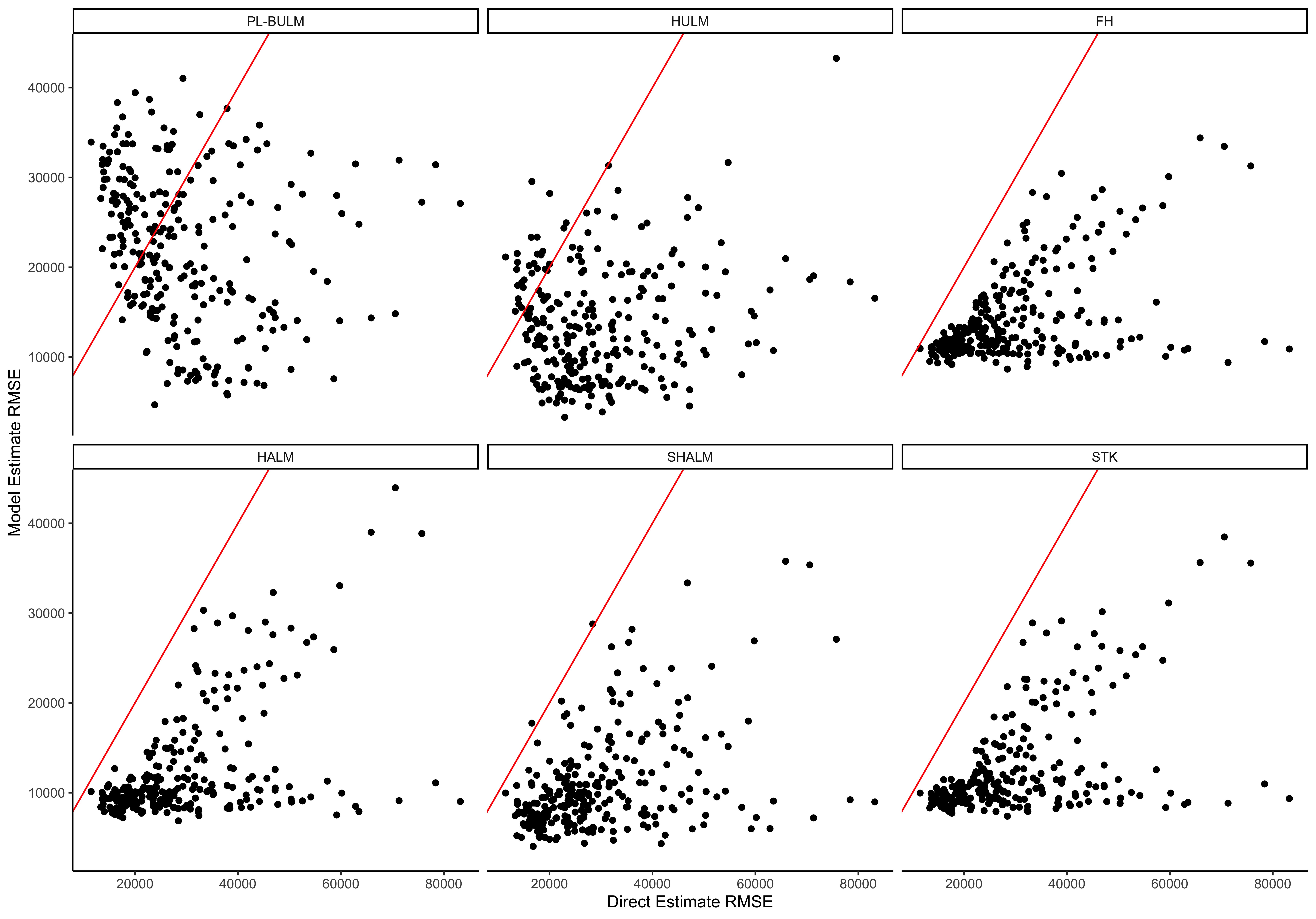
Figure 1: Empirical simulation results of Direct vs. Model-based RMSE by Public-Use Microdata Area (PUMA) for stratified random sampling using the 2018 1-year American Community Survey public-use microdata sample.

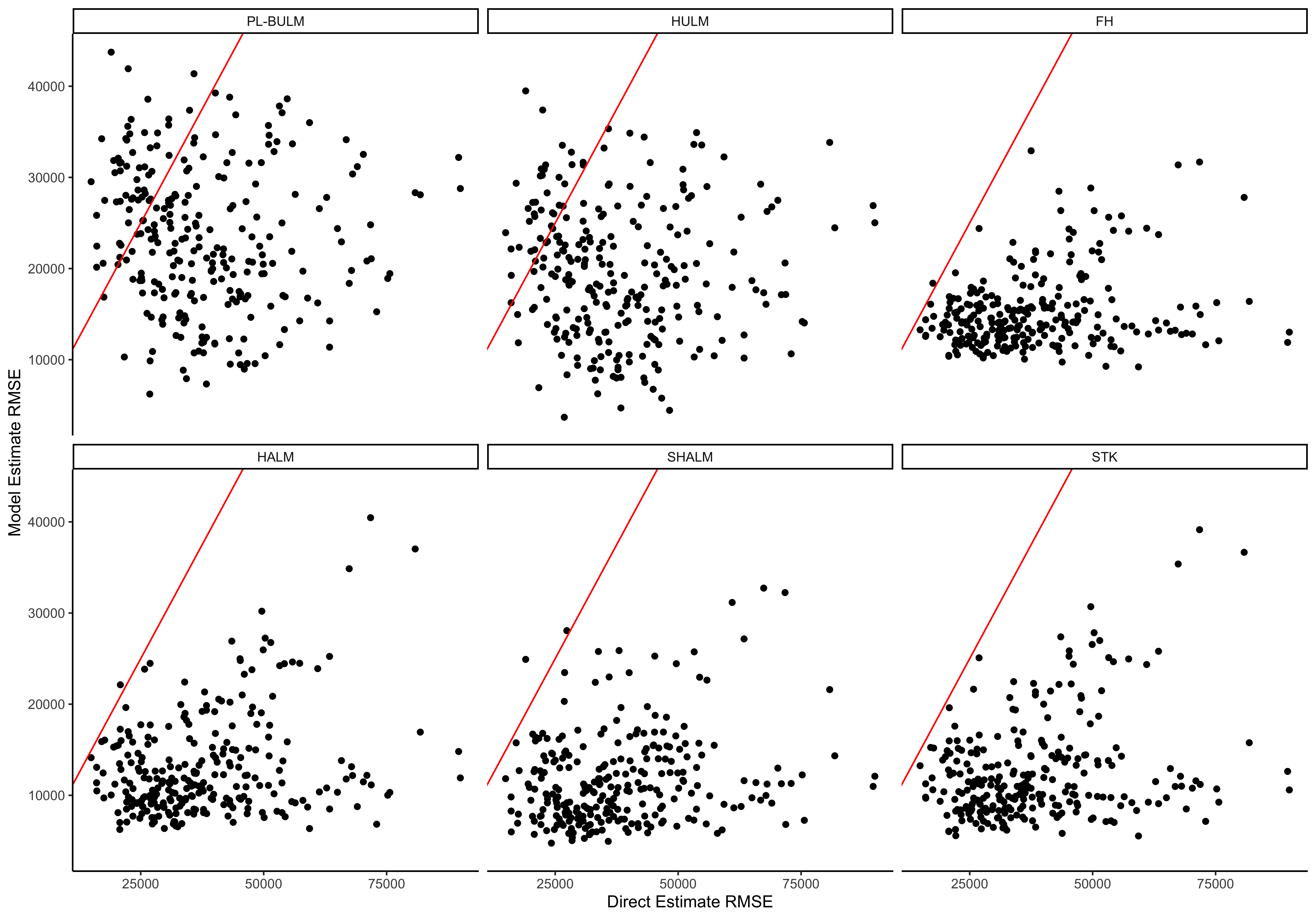
Figure 2: Empirical simulation results of Direct vs. Model-based RMSE by Public-Use Microdata Area (PUMA) for probability proportional to size sampling using the 2018 1-year American Community Survey public-use microdata sample.

Taken collectively, this simulation illustrates that heteroscedastic modeling techniques may be used to improve the quality of small area estimates. At the area level, these techniques may be used to simultaneously shrink both the design-based means as well as variances. At the unit-level, our framework allows for respondent specific variances when modeling continuous data. In both cases, our framework has the potential to improve the precision of associated small area estimates relative to approaches that do not have flexible models for the variance.

5 Analysis of American Community Survey Income Data

One important application of small area estimation techniques is estimation of mean or median income for various geographies. For example, the Small Area Income and Poverty Estimates Program (SAIPE) produces income estimates for all U.S. states and counties (Bell et al.,, 2016). In many cases, the estimates produced by SAIPE or similar programs may be used to allocate critical federal aid. Thus, improving the quality of model-based estimates for various outcomes such as income constitutes an important research problem. To this end, we demonstrate an application of our proposed SHALM approach by estimating the average income by PUMA for the state of California using the 2018 1-year ACS PUMS sample. The SHALM is fit analogously to Section 4, with the exception that the entire PUMS dataset was used rather than a subsample.

The model-based estimates of mean income by PUMA are shown in Figure 3, along with their standard errors. The estimates are generally as expected with higher incomes around city centers with high cost of living, such as the San Francisco Bay area and Los Angeles, and lower incomes in more rural parts of the state. Uncertainty is higher in areas that had lower sample sizes, but also in some areas with very high estimated income. For these counties, there was considerably more spread in the observed incomes, which contributes to the uncertainty around the estimated mean.

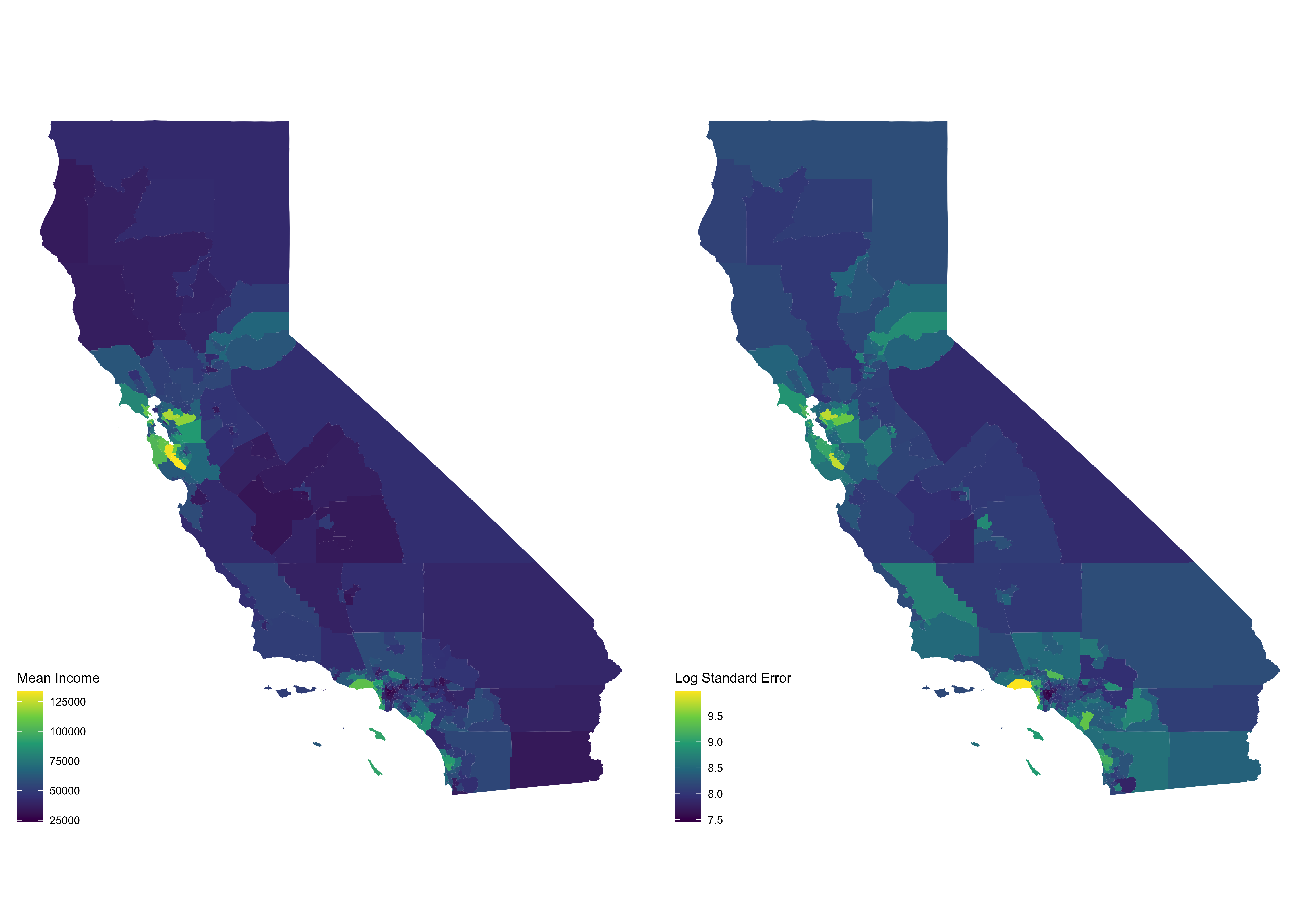
Figure 3: Model-based estimates of mean income by public use microdata area along with associated log transformed standard errors. Estimates are constructed using the 2018 1-year American Community Survey Public Use Microdata Sample.

We also compare the model-based estimates to the direct estimates in Figure 4. Here, we see that the two estimates generally agree, with points falling close to the one-to-one line. However, we also see that the model-based approach tends to result in slightly higher estimates for areas with low average income and slightly lower estimates for areas that exhibited high average income.

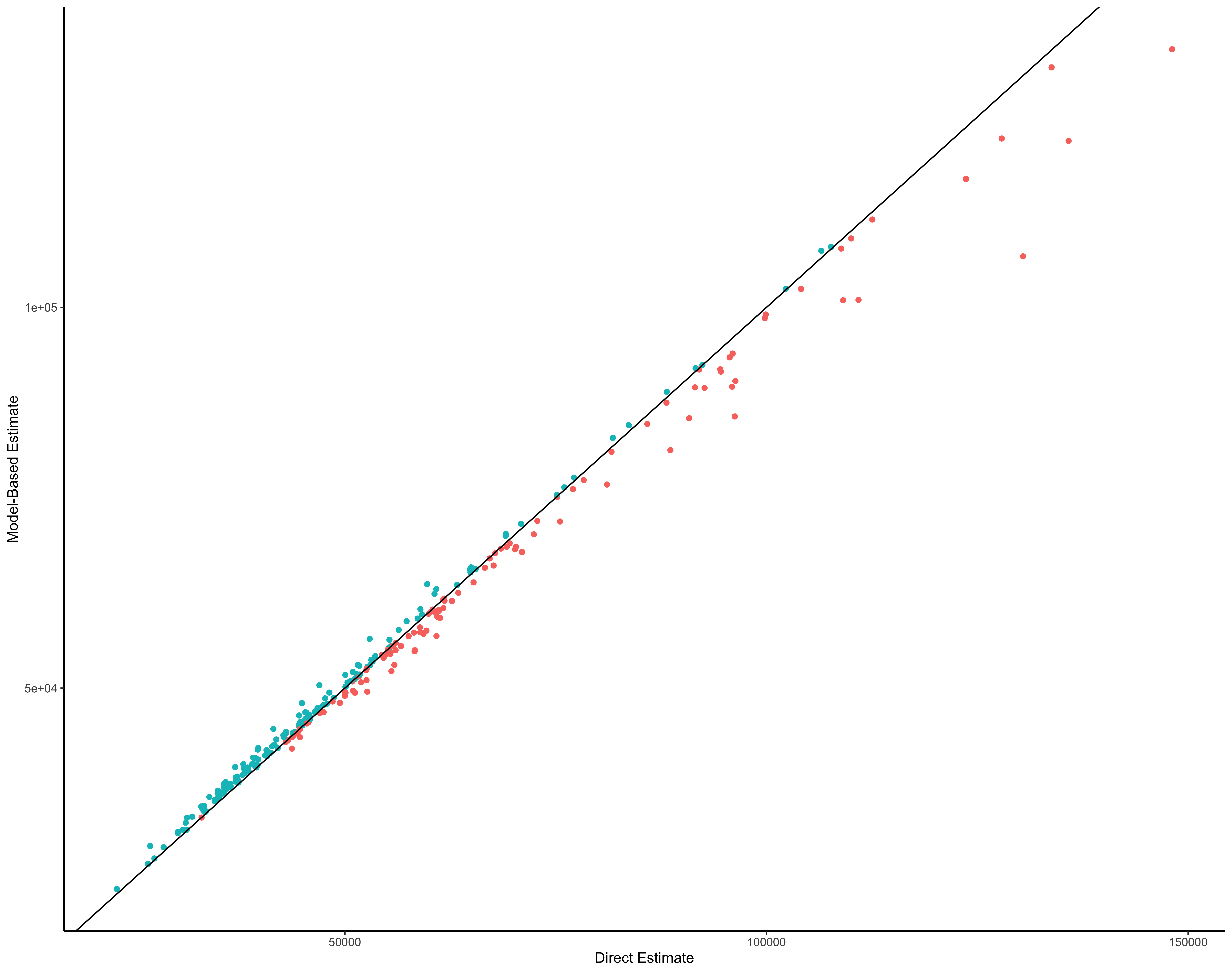
Figure 4: Direct vs. Model-based estimates of mean income by public use microdata area. Estimates are constructed using the 2018 1-year American Community Survey Public Use Microdata Sample.

6 Discussion

Small area/domain estimation is an area of wide-spread interest both for data users and official statistical agencies. Consequently, there has been significant research on both area-level and unit-level models with the goal of improving the precision of target estimates. Nevertheless, model-based approaches typically focus on modeling the mean, with a few notable exceptions. As illustrated here, in the presence of heteroscedasticity, simultaneously modeling both the mean and variance can achieve estimates with both reduced MSE and superior frequentist coverage properties.

By extending Bradley et al., (2020) and Parker et al., (2021), our approach to simultaneously modeling the mean and variance produces fully conjugate updates for hard-to-estimate parameters and is, therefore, extremely computationally efficient. Importantly, our approach is extremely flexible and allows for the incorporation of spatial dependence and covariates in the portion of the model for the variance.

Although our main focus is on area-level modeling, we also introduce unit-level models that account for informative sampling through the use of the pseudo-likelihood. These models can be extremely effective in situations where tabulations are desired for custom-geographies and/or situations when internal aggregation consistency is desired.

Our motivating example focused on modeling income and showcased the gains achieved from using our proposed approach. Nevertheless, for this example, our area-level models outperformed the models that were estimated at the unit-level. One reason for this is that the Gaussian assumption at the unit-level may not be an optimal starting point for this application due to data issues that arise from disclosure avoidance mechanisms. In this direction, there are several avenues for future work, including extensions to non-Gaussian data or Gaussian mixtures for both unit- and area-level models. In addition, future work also includes the extension to multivariate applications and applications where data integration is advantageous.

References

- Battese et al., (1988) Battese, G. E., Harter, R. M., and Fuller, W. A. (1988). “An error-components model for prediction of county crop areas using survey and satellite data.” Journal of the American Statistical Association, 83, 401, 28–36.
- Bell et al., (2016) Bell, W. R., Basel, W. W., and Maples, J. J. (2016). “An overview of the U. S. Census Bureau’s small area income and poverty estimates program.” In Analysis of Poverty Data by Small Area Estimation, ed. M. Pratesi, 349 – 378. New York: Wiley.
- Besag et al., (1991) Besag, J., York, J., and Mollié, A. (1991). “Bayesian image restoration, with two applications in spatial statistics.” Annals of the Institute of Statistical Mathematics, 43, 1, 1–20.
- Binder, (1983) Binder, D. A. (1983). “On the variances of asymptotically normal estimators from complex surveys.” International Statistical Review, 51, 3, 279–292.
- Bradley et al., (2020) Bradley, J. R., Holan, S. H., and Wikle, C. K. (2020). “Bayesian hierarchical models with conjugate full-conditional distributions for dependent data from the natural exponential family.” Journal of the American Statistical Association, 115, 532, 2037–2052.
- Bradley et al., (2018) Bradley, J. R., Holan, S. H., Wikle, C. K., et al. (2018). “Computationally efficient multivariate spatio-temporal models for high-dimensional count-valued data (with discussion).” Bayesian Analysis, 13, 1, 253–310.
- Bradley et al., (2016) Bradley, J. R., Wikle, C. K., and Holan, S. H. (2016). “Bayesian spatial change of support for count-valued survey data with application to the American Community Survey.” Journal of the American Statistical Association, 111, 514, 472–487.
- Brewer et al., (1984) Brewer, K., Early, L., and Hanif, M. (1984). “Poisson, modified Poisson and collocated sampling.” Journal of Statistical Planning and Inference, 10, 1, 15–30.
- Chen and Dunson, (2003) Chen, Z. and Dunson, D. B. (2003). “Random effects selection in linear mixed models.” Biometrics, 59, 4, 762–769.
- Fay III and Herriot, (1979) Fay III, R. E. and Herriot, R. A. (1979). “Estimates of income for small places: an application of James-Stein procedures to census data.” Journal of the American Statistical Association, 74, 366a, 269–277.
- Gladish et al., (2014) Gladish, D. W., Wikle, C., and Holan, S. (2014). “Covariate-based cepstral parameterizations for time-varying spatial error covariances.” Environmetrics, 25, 2, 69–83.
- Gneiting and Raftery, (2007) Gneiting, T. and Raftery, A. E. (2007). “Strictly proper scoring rules, prediction, and estimation.” Journal of the American Statistical Association, 102, 477, 359–378.
- Maiti et al., (2014) Maiti, T., Ren, H., and Sinha, S. (2014). “Prediction error of small area predictors shrinking both means and variances.” Scandinavian Journal of Statistics, 41, 3, 775–790.
- Maples et al., (2009) Maples, J., Bell, W., and Huang, E. T. (2009). “Small area variance modeling with application to county poverty estimates from the American Community Survey.” In Proceedings of the Section on Survey Research Methods, Alexandria, VA: American Statistical Association, 5056–5067.
- Marhuenda et al., (2013) Marhuenda, Y., Molina, I., and Morales, D. (2013). “Small area estimation with spatio-temporal Fay–Herriot models.” Computational Statistics & Data Analysis, 58, 308–325.
- Parker et al., (2021) Parker, P. A., Holan, S. H., and Wills, S. A. (2021). “A general Bayesian model for heteroskedastic data with fully conjugate full-conditional distributions.” Journal of Statistical Computation and Simulation, 91, 15, 3207–3227.
- Parker et al., (2019) Parker, P. A., Janicki, R., and Holan, S. H. (2019). “Unit level modeling of survey data for small area estimation under informative sampling: A comprehensive overview with extensions.” arXiv preprint arXiv:1908.10488.
- Polettini, (2017) Polettini, S. (2017). “A generalised semiparametric Bayesian Fay–Herriot model for small area estimation shrinking both means and variances.” Bayesian Analysis, 12, 3, 729–752.
- Porter et al., (2015) Porter, A. T., Wikle, C. K., and Holan, S. H. (2015). “Small area estimation via multivariate Fay–Herriot models with latent spatial dependence.” Australian & New Zealand Journal of Statistics, 57, 1, 15–29.
- Pourahmadi, (1999) Pourahmadi, M. (1999). “Joint mean-covariance models with applications to longitudinal data: Unconstrained parameterisation.” Biometrika, 86, 3, 677–690.
- Pourahmadi, (2011) — (2011). “Covariance estimation: The GLM and regularization perspectives.” Statistical Science, 26, 3, 369–387.
- Pourahmadi, (2013) — (2013). High-dimensional covariance estimation: with high-dimensional data, vol. 882. John Wiley & Sons.
- Savitsky and Gershunskaya, (2022) Savitsky, T. D. and Gershunskaya, J. (2022). “Bayesian Nonparametric Joint Model For Domain Point Estimates and Variances Under Biased Observed Variances.” Journal of Survey Statistics and Methodology.
- Savitsky and Toth, (2016) Savitsky, T. D. and Toth, D. (2016). “Bayesian estimation under informative sampling.” Electronic Journal of Statistics, 10, 1, 1677–1708.
- Schmidt et al., (2011) Schmidt, A. M., Guttorp, P., and O’Hagan, A. (2011). “Considering covariates in the covariance structure of spatial processes.” Environmetrics, 22, 4, 487–500.
- Skinner, (1989) Skinner, C. J. (1989). “Domain means, regression and multivariate analysis.” In Analysis of Complex Surveys, eds. C. J. Skinner, D. Holt, and T. M. F. Smith, chap. 2, 80 – 84. Chichester: Wiley.
- Sugasawa et al., (2017) Sugasawa, S., Tamae, H., and Kubokawa, T. (2017). “Bayesian estimators for small area models shrinking both means and variances.” Scandinavian Journal of Statistics, 44, 1, 150–167.
- Sun et al., (2022) Sun, A., Parker, P. A., and Holan, S. H. (2022). “Analysis of Household Pulse Survey Public-Use Microdata via Unit-Level Models for Informative Sampling.” Stats, 5, 1, 139–153.
- You, (2021) You, Y. (2021). “Small area estimation using Fay-Herriot area level model with sampling variance smoothing and modeling.” Survey Methodology, 47, 2, 361–371.
- You and Chapman, (2006) You, Y. and Chapman, B. (2006). “Small area estimation using area level models and estimated sampling variances.” Survey Methodology, 32, 1, 97.