Computing geometric feature sizes
for algebraic manifolds

Abstract

We introduce numerical algebraic geometry methods for computing lower bounds on the reach, local feature size, and the weak feature size of the real part of an equidimensional and smooth algebraic variety using the variety’s defining polynomials as input. For the weak feature size, we also show that non-quadratic complete intersections generically have finitely many geometric bottlenecks, and describe how to compute the weak feature size directly rather than a lower bound in this case. In all other cases, we describe additional computations that can be used to determine feature size values rather than lower bounds. We also present homology inference experiments that combine persistent homology computations with implemented versions of our feature size algorithms, both with globally dense samples and samples that are adaptively dense with respect to the local feature size.

1 Introduction

Exploring the geometry of a given data set has proven to be a powerful tool in data analysis. For example, topological data analysis (TDA) aims to recover topological information of a data set such as connectedness or holes in its shape [20, 27, 43] and has been successfully applied to problems in a wide range of fields [44, 53, 71]. If the data set lies on a manifold that is algebraic, namely it lies on a geometric shape defined by algebraic equations, a more direct approach using computational algebraic geometry can be applied. In this case, the data set can be viewed as a sampling of the algebraic manifold, as shown in Figure 1, where it is important to find guarantees that the topology of the sample, i.e., the topology of the Vietoris-Rips complex defined by the data set (see Definition 2.6) correctly estimates the topology of the underlying algebraic manifold.

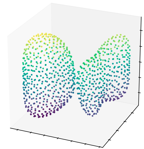
Figure 1: Dense sample from a quartic surface.

Topological and geometric data analysis algorithms frequently supply some form of the following guarantee: given a “dense enough” point sample from a space $X\subseteq\mathbb{R}^{n}$ as input, the algorithm correctly computes some geometric or topological property of $X$. The required density can be expressed in terms of certain invariants of the space $X$. The two most studied invariants are the reach, introduced by Federer [39], and the weak feature size, introduced by Grove and Shiohama in the context of Riemannian geometry [45, 46] and significantly expanded upon by Chazal and Lieutier for use in computational geometry [25]. These invariants are of considerable importance for persistent homology and reconstruction methods [4, 18, 25, 26, 29, 33, 56, 62].

In most settings, geometric feature sizes can only be estimated since a full specification of the space $X$ is not available. As a result, few examples of fully specified spaces with explicitly computed weak feature size have previously appeared. Algorithms computing these invariants and thus geometrical theories for efficient computations are an important area of study in applied geometry. This paper aims at providing some answers in this direction using numerical algebraic geometric methods, e.g. see [10, 67].

Throughout this paper, nonempty and compact algebraic manifolds $X=V(F)\cap\mathbb{R}^{n}$ are considered, where $F=\{f_{1},f_{2},\dots,f_{m}\}$ is a system consisting of polynomials in $\mathbb{R}[x_{1},\dots,x_{n}]$ and $V(F)=\{x\in\mathbb{C}^{n}~{}|~{}F(x)=0\}.$ Section 2 presents necessary background on feature sizes, persistent homology, and homology inference. The distance-to-X function $d_{X}:\mathbb{R}^{n}\to\mathbb{R}$, defined as $d_{X}(z)=\inf_{x\in X}\|x-z\|,$ is not differentiable everywhere in $\mathbb{R}^{n}$ for most spaces $X$. Grove [45] constructs an analog of Morse theory defining critical points of $d_{X}$ or geometric bottlenecks of $X$ as those points $z\in\mathbb{R}^{n}\setminus X$ which are in the convex hull of their closest points on $X$. The weak feature size is the infimum of all the critical values of $d_{X}$. The critical values of $d_{X}$ are those values $d_{X}(z)$ where $z$ is a geometric bottleneck (see Definition 2.3).

Example.

Consider the ellipsoid $X\subseteq\mathbb{R}^{3}$ defined by $x_{1}^{2}+x_{2}^{2}+x_{3}^{2}/2=1$ as depicted in Figure 2. It has a single geometric bottleneck at the origin (red point).

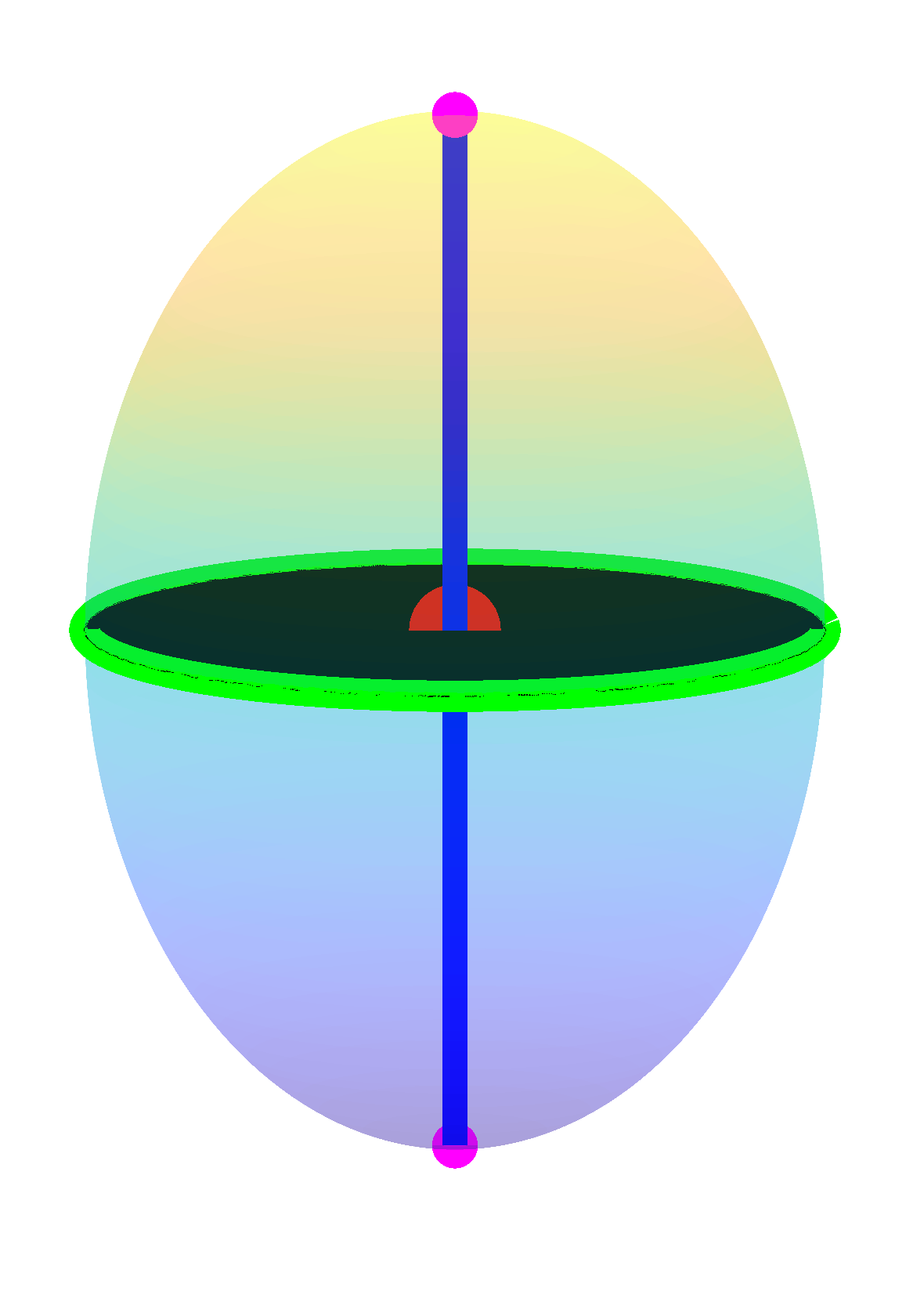
Figure 2: Ellipsoid

We will see in Section 4 that the number of convex hulls of closest points which contain a geometric bottleneck crucially impacts computations. The ellipsoid in Figure 2 is an example that poses difficulties, as it has a one-dimensional locus of convex hulls along the $(x_{1},x_{2})$-plane which contain the origin. They are depicted with black segments connecting green antipodal points on the unit circle in the $(x_{1},x_{2})$-plane.

Algebraic conditions also detect that the origin is contained in the convex hull of its furthest points on $X$, which lies along the $x_{3}$-axis with blue segments connecting the magenta points at $\left(0,0,\pm\sqrt{2}\right)$ in Figure 2.

Using a combination of geometric arguments, the Tarski-Seidenberg Theorem, and Sard’s Theorem, Fu proved that the set of critical values of $d_{X}$ is finite when $X$ is semialgebraic [41]. This implies that the weak feature size is always positive. In the ellipsoid example, the weak feature size is $1$. This theorem strongly motivates studying the weak feature size as it applies even when $X$ is not smooth nor equidimensional. The proof, however, does not suggest a feasible algorithm for computing the critical values of $d_{X}$.

In Section 3, we describe a method to compute the reach of $X$ as well as the local feature size [3] of $X$ at a point $w\in\mathbb{R}^{n}$ given the defining polynomials $F$ as input. Numerical computations can compute these quantities to arbitrary precision via our approach. Moreover, if the input depends on rational numbers, exactness recovery methods such as [8] can refine the numerical results to extract exact information. For example, we use exactness recovery methods in Example 2.4 to determine exact expressions for the reach of a particular space.

Theorem (3.5, 3.6).

For both the reach and the local feature size, one can utilize the finite set of points computed via a single parameter homotopy [59] on a polynomial system constructed using first-order critical conditions to obtain a nontrivial lower bound. Using additional reality testing, one can determine the value of the reach and the local feature size.

To the best of our knowledge, these provide the first algorithms that can compute these quantities for algebraic manifolds of arbitrary codimension.

Section 4 is dedicated to constructing a theory and algorithms for computing the weak feature size. We apply a wholly algebraic framework to this problem when $X$ is the real part of a smooth and equidimensional algebraic variety. The resulting theory yields an alternative proof of Fu’s Theorem in this setting as well as a method for computing bounds on the weak feature size.

Theorem (4.8, 4.10).

A lower bound on the weak feature size can be obtained using the union of the finite set of points computed via $n$ parameter homotopies [59]. Using additional reality testing, one can determine the value of the weak feature size.

Example.

The ellipsoid example above has a geometric bottleneck with infinitely many closest points. Although the previous theorem applies to that case, it is often more desirable from a numerical conditioning standpoint to consider nonsingular isolated solutions to well-constrained systems. Consider the perturbation defined by $x^{2}+y^{2}+z^{2}/2\color[rgb]{0,0,1}+xz/7=1$, illustrated in Figure 3. In this case, only three convex hulls containing the geometric bottleneck at the origin contribute to algebraic computations. Black segments connect the origin to green points, which are distance minimizers.

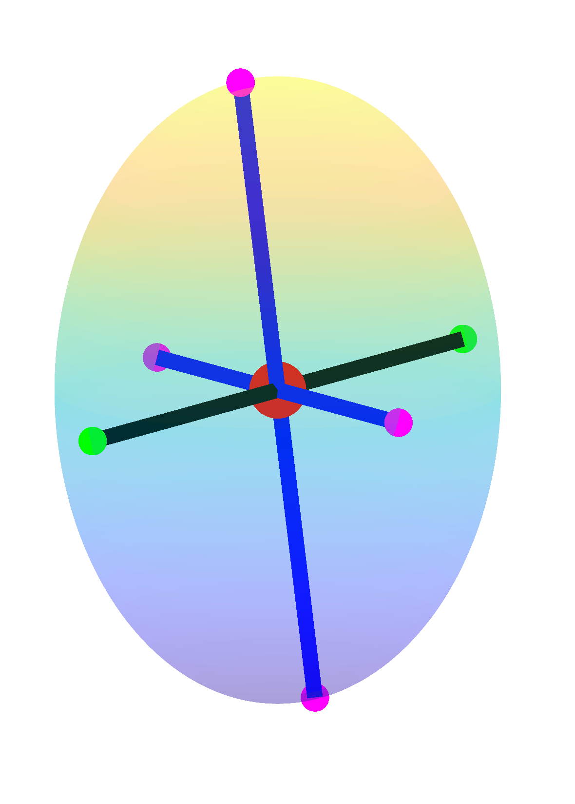
Figure 3: Perturbation of ellipsoid

This example’s behavior is the typical result of a perturbation in a rigorous sense. By applying the celebrated Alexander-Hirschowitz Theorem [2] on the expected dimension of the secant variety of the Veronese embedding, one obtains a description of the generic behavior of geometric bottlenecks as summarized in the following.

Theorem (4.15).

Non-quadratic generic complete intersections have finitely many critical points, i.e., finitely many geometric bottlenecks.

As a consequence, we construct algorithms using homotopy continuation to compute the weak feature size with arbitrary precision. Examples are presented in Section 5. A Julia package which implements these algorithms for general use via HomotopyContinuation.jl [17] is available at https://github.com/P-Edwards/HomologyInferenceWithWeakFeatureSize.jl. We also use Bertini [11] implementations. Data, scripts, and input files for all examples are available at https://github.com/P-Edwards/wfs-and-reach-examples.

Our feature size algorithms comprise the final missing component of a homology inference pipeline that combines feature size computations, sampling methods for algebraic varieties [34, 36], and persistent homology algorithms [12, 24, 29, 30]. In Section 6, we present homology inference results from an implemented version of this pipeline. Our feature size computations also provide a previously unavailable baseline to investigate the performance of methods which estimate feature sizes. As a proof of concept, we consider an “adaptive” subsampling method for persistent homology proposed by Dey et al. [33] that estimates local feature sizes. Their approach has recently been expanded to a general framework for adaptive subsampling by Cavanna and Sheehy [22, 23]. Using feature sizes computed via our new algorithms, we find evidence that the method of Dey et al. performs comparably to a baseline analog of Chazal and Lieutier [26] which requires directly computed local feature sizes.

1.1 Related work

Recent work on computing feature sizes in the algebraic setting mostly focused on computing lower bounds for the reach, motivated by a result of Amari et al. [1, Thm. 3.4] which shows the reach of a compact manifold is determined by two distinct types of geometric behavior: regions of high curvature and “bottleneck structures,” which we call “geometric 2-bottlenecks” (Definition 4.1). Breiding and Timme [16] observed that a straightforward computation can find the maximal curvature of an implicitly defined plane curve and Horobeţ [54] studied the problem in greater generality by investigating an algebraic variety’s critical curvature degree. Horobeţ and Weinstein [55] studied related theoretical problems in the context of “offset filtrations” and, in particular, showed that the reach is algebraic over $\mathbb{Q}$ for real algebraic manifolds defined by polynomials with rational coefficients. The third author [38] studied computing 2-bottlenecks with numerical algebraic geometry while Weinstein together with the first and third authors [35] developed formulas for the number of algebraic 2-bottlenecks of a smooth algebraic variety in terms of polar and Chern classes. A subset of the present manuscript’s authors [34] show the special case of Theorem 4.15 for 2-bottlenecks using a different approach.

Lowering the theoretical complexity of computing the Betti numbers and related invariants of semialgebraic sets from a list of defining polynomials comprises a rich and ongoing topic of study in real algebraic geometry, e.g., the references [5, 6, 18] more extensively characterize recent progress in this area. The resulting algorithms are challenging to implement efficiently and, to the best of our knowledge, no general implementations are available. We take a distinct approach to homology inference that is complimentary by focusing on producing efficient implementations rather than lowering complexity bounds.

2 Background and Preliminaries

The following summarizes the elements from the theory of distance functions and geometric feature sizes, particularly for semi-algebraic sets, necessary to state our results. We also recall how to combine feature size information with the “persistent homology pipeline” to compute the Betti numbers (with field coefficients) of a subspace of $\mathbb{R}^{n}$.

2.1 Distance functions and geometric feature sizes

In this paper, the distance between two points $x,z\in\mathbb{R}^{n}$ uses the Euclidean distance:

$$d(x,z)=\|x-z\|=\sqrt{\sum_{i=1}^{n}(x_{i}-z_{i})^{2}}.$$

For any nonempty subset $S\subseteq\mathbb{R}^{n}$, let $d_{S}:\mathbb{R}^{n}\to\mathbb{R}$ denote the distance-to-$S$ function, namely $d_{S}(z)=\inf_{s\in S}\|s-z\|$. For any non-negative $\varepsilon$, let $S^{\epsilon}=d_{S}^{-1}[0,\epsilon]$ be the union of all closed $\epsilon$-balls centered at points of $S$. For a nonempty and compact subset $X\subseteq\mathbb{R}^{n}$ and for any $z\in\mathbb{R}^{n}$, let $\pi_{X}(z)=\{x\in X~{}|~{}d_{X}(z)=d(x,z)\}$ be the set of the points in $X$ with minimal distance to $z$.

Definition 2.1.

The medial axis of $X$ is

$$\mathcal{M}_{X}=\overline{\{z\in\mathbb{R}^{n}~{}|~{}\#\pi_{X}(z)>1\}}\text{.}$$

Equivalently, $\mathcal{M}_{X}$ is the (Euclidean) closure of the set of points in $\mathbb{R}^{n}$ that have at least $2$ closest points in $X$.

Naturally, one can consider subsets of the medial axis based on the number of closest points. That is, for $k\geq 2$, $\mathcal{M}_{X,k}=\overline{\{z\in\mathbb{R}^{n}~{}|~{}\#\pi_{X}(z)\geq k\}}$ is the $k$-medial axis where $\mathcal{M}_{X}=\mathcal{M}_{X,2}$, i.e., the medial axis is the $2$-medial axis.

Definition 2.2.

The function $d_{\mathcal{M}_{X}}:\mathbb{R}^{n}\to\mathbb{R}\cup\{\infty\}$ is also called the local feature size function of $X$ [3], denoted $\operatorname{lfs}$. For $w\in\mathbb{R}^{n}$, $\operatorname{lfs}(w)$ is the local feature size at $w$. The function $\operatorname{lfs}$ takes value $\infty$ if $\mathcal{M}_{X}=\emptyset$, e.g., if $X$ is convex. The reach of $X$ [39] is defined as

$$\tau_{X}=\min_{x\in X}\operatorname{lfs}(x)\text{.}$$

Definition 2.3.

A point $z\in\mathbb{R}^{n}\setminus X$ is a critical point of $d_{X}$ [45, 46] or a geometric bottleneck of $X$ if $z$ is in the convex hull of $\pi_{X}(z)$. The weak feature size [25] of $X$ is defined as:

$$\operatorname{wfs}(X)=\inf_{z\in\operatorname{crit}(d_{X})}~{}d_{X}(z)$$

where $\operatorname{crit}(d_{X})$ denotes the set of critical points of $d_{X}$.

Notice that $\operatorname{crit}(d_{X})$ is a subset of $\mathcal{M}_{X}$, so that $\tau_{X}\leq\operatorname{wfs}(X)$. Also notice that the above condition can be phrased in terms of well-centered simplices. The convex hull of a set of at most $n+1$ affinely independent points in $\mathbb{R}^{n}$ is a well-centered simplex if its circumcenter lies in its interior [68]. A point $z\in\mathbb{R}^{n}\setminus X$ is a geometric bottleneck of $X$ if it is the circumcenter of a well-centered simplex with vertices in $\pi_{X}(z)$.

Example 2.4.

To illustrate the previous definitions, consider the plane curve $C\subseteq\mathbb{R}^{2}$ defined by $d(x,p_{1})^{2}\cdot d(x,p_{2})^{2}=2$ where $p_{1}=(1,0)$ and $p_{2}=(-1,0)$. The curve $C$ is called a Cassini oval with 2 foci and shown in Figure 4(a) along with its medial axis (cyan curve) and bottlenecks (red points). These types of curves, with a concentration on examples bearing more resemblance to an ellipse than the one we consider, were proposed by Cassini in the late $17^{\rm th}$ century as candidates for planetary orbits [21, p. 36]. The medial axis $\mathcal{M}_{C}$ consists of three segments along the coordinate axes, namely

$$\begin{array}[]{l}(a,0)\hbox{~{}~{}~{}for~{}~{}~{}}a\in\left[-\sqrt{2\sqrt{2}-2},\sqrt{2\sqrt{2}-2}\right]\hbox{~{}~{}~{}and~{}~{}~{}}\\[7.22743pt] (0,b)\hbox{~{}~{}~{}for~{}~{}~{}}b\in\left(-\infty,-\sqrt{2\sqrt{2}+2}\right]\cup\left[\sqrt{2\sqrt{2}+2},\infty\right).\end{array}$$

The reach is $\tau_{C}=\sqrt{\sqrt{2}-1}\approx 0.6436$ attained at the origin and $\left(\pm\sqrt{2\sqrt{2}-2},0\right)$. There are three bottlenecks, namely the origin and $(\pm\sqrt{1/2},0)$ each with two closest points in $C$, with the weak feature size being $\operatorname{wfs}(C)=\sqrt{\sqrt{2}-1}$ attained at the origin. Hence, $\tau_{C}=\operatorname{wfs}(C)$.

Similarly, consider the plane curve $C^{\prime}\subseteq\mathbb{R}^{2}$ defined by $d(x,r_{1})^{2}\cdot d(x,r_{2})^{2}\cdot d(x,r_{3})^{2}=2$ where $r_{1}=(1,0)$, $r_{2}=(-1/2,\sqrt{3}/2)$, and $r_{3}=(-1/2,-\sqrt{3}/2)$. The curve $C^{\prime}$ is called a Cassini oval with 3 foci and is shown in Figure 4(b) along with its medial axis (cyan curve) and bottleneck (red point) at the origin which has three closest points in $C^{\prime}$. The reach is

$$\tau_{C^{\prime}}=\dfrac{\sqrt[3]{64-26\sqrt{2}}}{7}\approx 0.4298$$

attained at the three points on the end of the medial axis in the interior of $C^{\prime}$. The weak feature size is $\operatorname{wfs}(C^{\prime})=\sqrt[3]{\sqrt{2}-1}\approx 0.7454$ attained at the origin. Hence, $\tau_{C^{\prime}}<\operatorname{wfs}(C^{\prime})$.

We note that the exact values for the reach were computed by using the results of the numerical computation in Example 3.7 together with the exactness recovery method in [8] yielding minimal polynomials of $x^{4}+2x^{2}-1$ and $343x^{6}-128x^{3}+8$ for $\tau_{C}$ and $\tau_{C^{\prime}}$, respectively. Hence, the algebraic degree of the reach is $4$ and $6$, respectively.

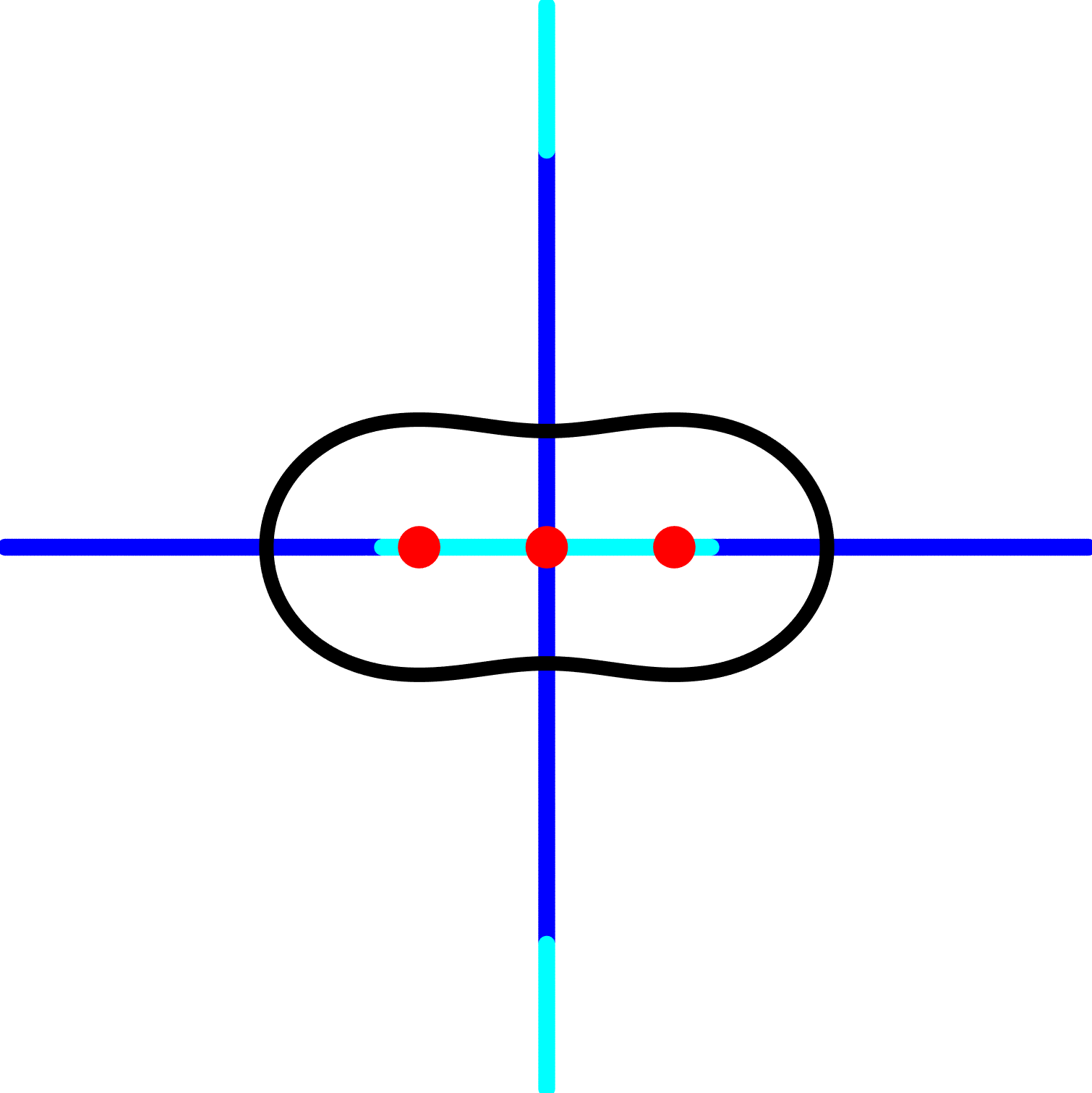
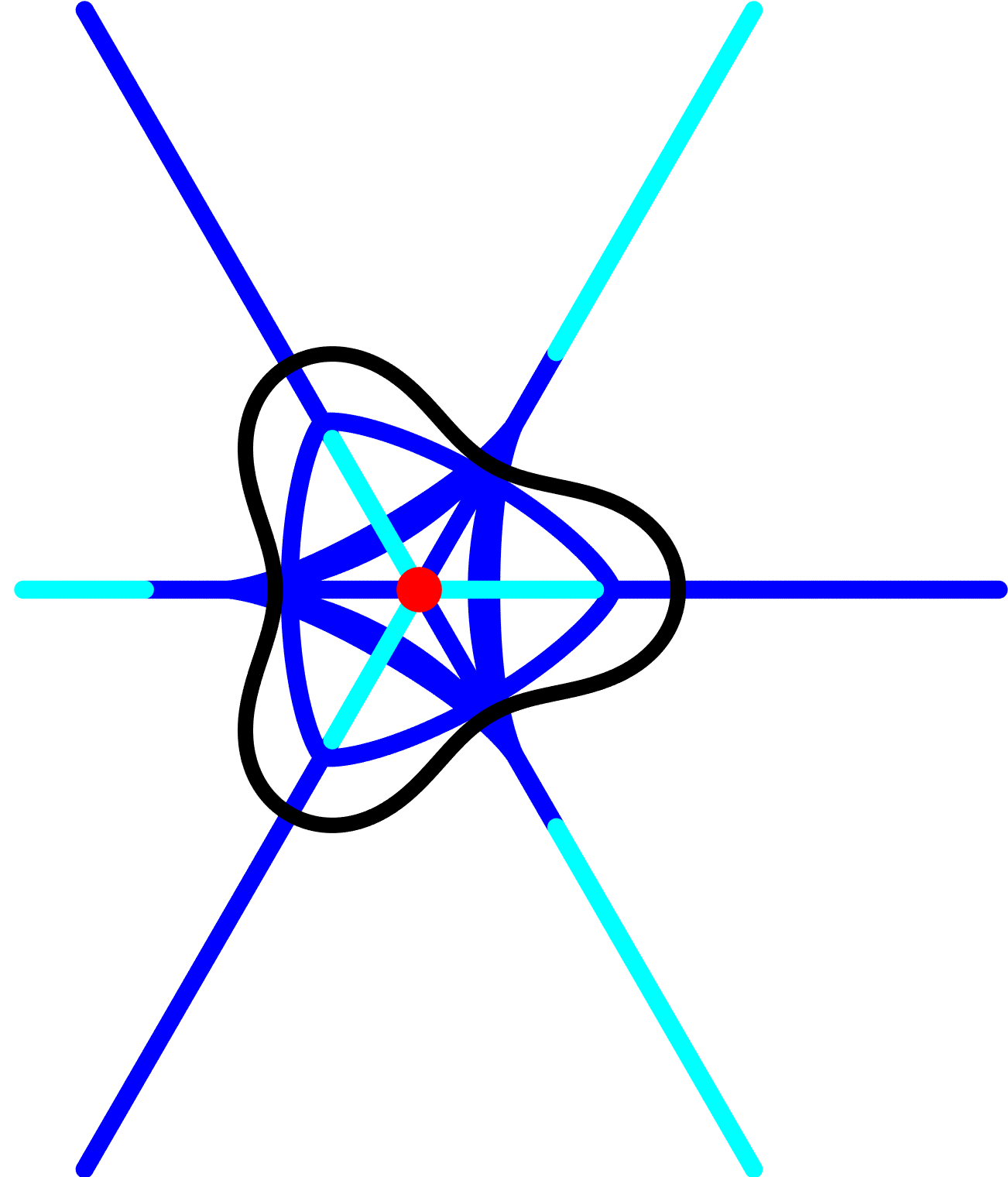
(a)		(b)

Figure 4: Black curve is the Cassini oval with (a) 2 foci and (b) 3 foci. The red points are geometric bottlenecks and the union of the cyan curves form the medial axis.

The following results show that distance functions $d_{X}:\mathbb{R}^{n}\to\mathbb{R}$ enjoy some properties similar to Morse functions in Morse theory [61] and justify studying the weak feature size in the algebraic setting. For the sake of analogy, recall that if $f:M\to\mathbb{R}$ is a Morse function on a compact manifold $M$ with critical points $C_{f}$ then, by a theorem of A. Morse [60] and Sard [65], $f(C_{f})$ is finite. By a fundamental theorem of Morse theory (see, e.g., [58, Thm. 3.1]), if $f(C_{f})\cap[r_{1},r_{2}]=\emptyset$ then $f^{-1}(-\infty,r_{1}]$ is a deformation retract of $f^{-1}(-\infty,r_{2}]$.

Theorem 2.5.

Let $X$ be a nonempty and compact subset of $\mathbb{R}^{n}$, $B$ be the set of geometric bottlenecks of $X$, and $\epsilon$ and $\epsilon^{\prime}$ satisfy $0<\epsilon\leq\epsilon^{\prime}$.

• (Grove, 1993 [45, Prop. 1.8]) If $d_{X}(B)\cap[\epsilon,\epsilon^{\prime}]=\emptyset$, then $d_{X}^{-1}[\epsilon,\epsilon^{\prime}]$ is homeomorphic to $d_{X}^{-1}(\epsilon)\times[\epsilon,\epsilon^{\prime}]$. In particular, if $\epsilon^{\prime}<\operatorname{wfs}(X)$, then the thickening $X^{\epsilon}$ is a deformation retract of $X^{\epsilon^{\prime}}$.

• (Fu, 1985 [41, §5.3]) If $X$ is semialgebraic, then $d_{X}(B)$ is finite, and so $\operatorname{wfs}(X)>0$.

• Any compact and semialgebraic set $X$ is a deformation retract of $X^{\epsilon}$ for some sufficiently small $\epsilon>0$. We can conclude this in the following way. If $X$ is semialgebraic and bounded, i.e., $X$ is contained in a Euclidean ball of finite radius in $\mathbb{R}^{n}$, then $X$ is finitely triangulable [57, Thm. 3]. Since any compact and finitely triangulable set is an absolute neighborhood retract (ANR) [47, Cor. 3.5], any compact semialgebraic set $X$ is an ANR. For any compact ANR $X$, $X$ is a deformation retract of $X^{\epsilon}$ for some sufficiently small $\epsilon>0$.

The Morse Lemma implies that the set of critical points of a Morse function on a compact manifold is finite (see, e.g., [58, Cor. 2.3]). Nonetheless, the distance-to-$X$ function $d_{X}$ need not always have finitely many geometric bottlenecks even if $X$ is smooth, compact, and an algebraic subset of $\mathbb{R}^{n}$ (see, e.g., Example 3.9). We consider this in more detail in Section 4.

2.2 Persistent homology and homology inference

In Section 6, we will consider a computational application combining algebraic computations for $\operatorname{lfs}$ and $\operatorname{wfs}$ with sampling algorithms (e.g., [34, 36]) and persistent homology to infer the Betti numbers of an algebraic manifold. In this context, the “persistent homology pipeline” starts with input in the form of a finite set of points $P\subseteq\mathbb{R}^{n}$ and computes the homology of simplicial complexes built from that input.

Definition 2.6.

Let $P\subseteq\mathbb{R}^{n}$ be a finite set of points and $\epsilon\geq 0$. The C̆ech complex for $P$ with parameter $\epsilon$, denoted $C_{P}(\epsilon)$, is the nerve of the set $\{\overline{B}_{p}(\epsilon)\}_{p\in P}$ where $\overline{B}_{x}(\epsilon)$ denotes the closed ball of radius $\epsilon$ with center $x$. The Vietoris-Rips complex, $R_{P}(\epsilon)$, is the simplicial complex $\{\sigma\subseteq P\mid\operatorname{diam}(\sigma)\leq\epsilon\}$. See, e.g., [37, §3.2] for details.

In practice, implemented versions of persistent homology (e.g., [12, 13]) use the Vietoris-Rips complex for computational reasons. For $0\leq\epsilon\leq\epsilon^{\prime}$, we have subcomplex inclusions $C_{P}(\epsilon)\hookrightarrow C_{P}(\epsilon^{\prime})$ and $R_{P}(\epsilon)\hookrightarrow R_{P}(\epsilon^{\prime})$. It is convenient to assemble these inclusions into functors $C_{P},R_{P}:\mathbf{R}\to\mathbf{simp}$ where $\mathbf{R}$ denotes the poset of real numbers with the standard ordering and $\mathbf{simp}$ the category of simplicial complexes with simplicial maps as morphisms. By taking the $\ell^{\rm th}$ homologies with ${\mathbb{F}}_{2}$ coefficients of the values of these functors, we obtain persistence modules which are functors $H_{\ell}C_{P},H_{\ell}R_{P}:\mathbf{R}\to\operatorname{\mathbf{vect}}_{{\mathbb{F}}_{2}}$. Each persistence module has an associated rank function which summarizes its algebraic structure.

Definition 2.7.

Let $M:\mathbf{R}\to\operatorname{\mathbf{vect}}_{\mathbb{Z}/2}$ be a functor and let $\mathbb{R}^{2}_{<}=\{(x,y)\in\mathbb{R}^{2}\mid x<y\}$. The rank function of $M$ is $\operatorname{rank}(M):\mathbb{R}^{2}_{<}\to\mathbb{Z}$ defined by $\operatorname{rank}(M)(x,y)=\operatorname{rank}(M(x\leq y))$.

A standard way to present the information in a rank function is via its persistence diagram. Let $\overline{\mathbb{R}}=\mathbb{R}\cup\{-\infty,\infty\}$ and let $\overline{\mathbb{R}}^{2}_{<}$ be defined similarly to $\mathbb{R}^{2}_{<}$.

Definition 2.8.

Let $M:\mathbf{R}\to\operatorname{\mathbf{vect}}_{{\mathbb{F}}_{2}}$ be a persistence module. The persistence diagram of $M$, if one exists, is the multiset $DM$ in $\overline{\mathbb{R}}^{2}_{<}$ where $\operatorname{rank}(M)(x,y)$ is the number of points in $DM$ strictly above and at least as far left as $(x,y)$ in $\overline{\mathbb{R}}^{2}_{<}$. The multiset $DM$ is called the persistence diagram of $M$.

The persistence modules we have discussed all have persistence diagrams and we assume the same for all persistence modules going forward. Note that this approach to defining persistence diagrams is somewhat non-standard for the sake of brevity. See, e.g., [64] for a more comprehensive approach. A point $(b,d)$ in $D(H_{\ell}R_{P})$ can be regarded as representing an $\ell$-dimensional homology feature which is “born” at radius $b$ and “dies” at radius $d$ as shown in Figure 5.

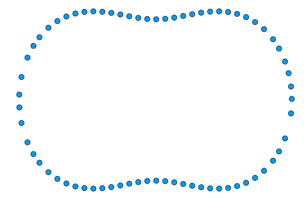
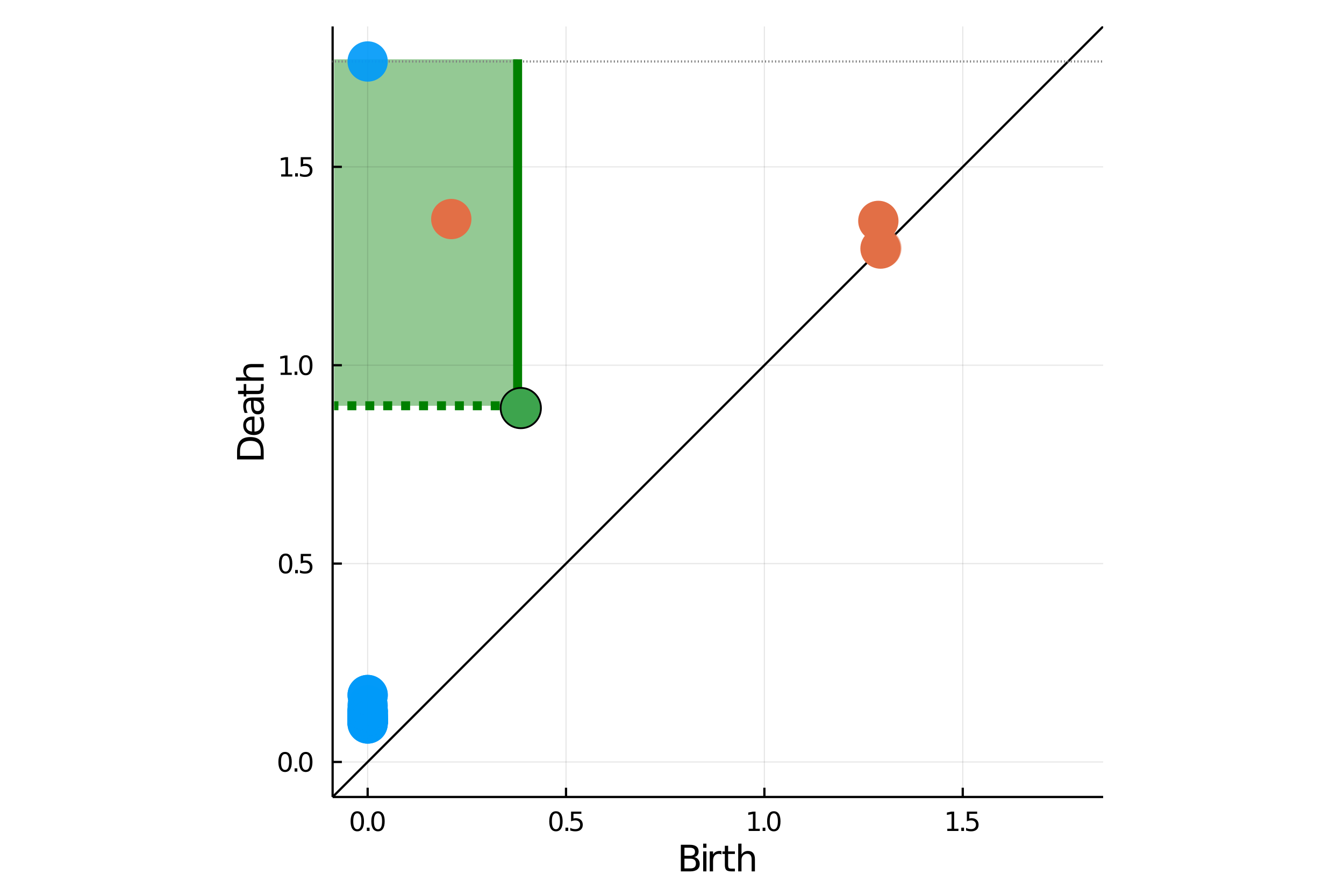
Figure 5: A sample from a curve and its Vietoris-Rips persistence diagram in degree 1 (red) and 0 (blue). The green region depicts inferred homology features as in Theorem 2.11.

One of the essential theoretical justifications for computing persistent homology is that the Vietoris-Rips persistence diagram of a “dense enough” point sample from a compact space $X\subseteq\mathbb{R}^{n}$ recovers the Betti numbers of $X$.

Definition 2.9.

Let $X,Y\subseteq\mathbb{R}^{n}$ be compact and $0\leq\delta\leq\epsilon$. The set $X$ is a $(\delta,\epsilon)$-sample of $Y$ if $X\subseteq Y^{\delta}$ and $X\subseteq Y^{\epsilon}$.

Theorem 2.10.

[25, 29, Homology Inference Theorem] Let $X,\hat{X}\subseteq\mathbb{R}^{n}$ such that $X$ is compact and semialgebraic and $\hat{X}$ is a $(\delta,\epsilon)$-sample of $X$. If $X^{2(\epsilon+\delta)}$ is homotopy equivalent to $X$, then $\operatorname{rank}(H_{\ell}C_{\hat{X}})(\epsilon,2\epsilon+\delta)$ is the $\ell^{\rm th}$ Betti number of $X$, $\beta_{\ell}(X)$. Equivalently, $\beta_{\ell}(X)$ is the number of points above and to the left of $(\epsilon,2\epsilon+\delta)$ in $D(H_{\ell}C_{\hat{X}})$.

There is also a version of this for Vietoris-Rips complexes. It follows directly from, e.g., [31, Thm 2.5], the Homology Inference Theorem, and an interleaving argument similar to Chazal and Lieutier’s proof of the Homology Inference Theorem [25]. A proof appears in Appendix A for the sake of completeness.

Theorem 2.11.

Let $A_{n}=\sqrt{\frac{2n}{n+1}}$, $\hat{X}$ be a $(\delta,\epsilon)$-sample of a semialgebraic set $X\subseteq\mathbb{R}^{n}$, and $\delta^{\prime}=2\epsilon(A_{n}^{2}-1)+\delta A_{n}$. If $2(\epsilon+\delta^{\prime})<\operatorname{wfs}(X)$ then, for $a(\delta,\epsilon)=2\epsilon$ and $b(\delta,\epsilon)=2(2\epsilon A_{n}+\delta)$, the $\ell^{\rm th}$ Betti number $\beta_{\ell}(X)$ is the rank of the map obtained from applying $H_{\ell}$ to the inclusion map $R_{\hat{X}}(a(\delta,\epsilon))\subseteq R_{\hat{X}}(b(\delta,\epsilon))$.

In the algebraic setting, we can construct the following “homology inference pipeline” (Algorithm 1) with persistent homology computations, provided we can compute weak feature sizes and samples of algebraic manifolds. The latter is possible with existing algorithms [34, 36].

Input : A polynomial system $F$ defining a smooth and equidimensional algebraic variety with $X=V(F)\cap\mathbb{R}^{n}$ compact and a degree of homology $\ell\geq 0$.

Output : A persistence diagram which encodes the $\ell^{\text{th}}$ $\mathbb{F}_{2}$-Betti number of $X$ along with additional information.

1 Compute $0<\omega<\operatorname{wfs}(X)$ ;

2 Compute using $\omega$ a $(\delta,\epsilon)$-sample of $X$, $\hat{X}$, which satisfies the assumptions of Theorem 2.11 ;

3 Compute (e.g., with Ripser [12]) and return the Vietoris-Rips persistence diagram of $\hat{X}$ ;

Algorithm 1 PH Homology Inference

3 Algebraic medial axis, reach, and local feature size

The geometric definition of the medial axis and hence the reach and local feature size in Section 2 utilize a semialgebraic condition via closest points. By replacing closest points with a criticality condition, the following provides an algebraic relaxation that is amenable to computational algebraic geometry over $\mathbb{C}$. As before, we assume that $X=V(F)\cap\mathbb{R}^{n}$ is nonempty and compact where $F$ is a polynomial system with real coefficients.

Definition 3.1.

Let $F=\{f_{1},\dots,f_{m}\}$ be a system of polynomials in $n$ variables with real coefficients such that $V(F)$ is equidimensional and smooth of codimension $c$. The medial axis correspondence of $F$, denoted $M(F)$, is the algebraic subset of $\mathbb{C}^{n}\times\mathbb{C}^{n}\times\mathbb{C}^{n}$ of points $(x_{1},x_{2},z)$ which satisfy the equations:

$$F(x_{1})=F(x_{2})=0,\ \ \ \text{rank}[x_{i}-z\ JF(x_{i})^{T}]\leq c\ \text{ for }i=1,2,\ \text{ and }d(x_{1},z)^{2}=d(x_{2},z)^{2}$$

where $JF(p)$ is the Jacobian matrix of $F$ evaluated at $p$. If $\Delta$ is the subset of points $(x_{1},x_{2},z)$ where any two of the entries are equal, the algebraic medial axis of $F$ is the closure of the image of the projection of $M(F)\setminus\Delta$ onto its third factor.

In particular, the condition $\text{rank}[x_{i}-z\ JF(x_{i})^{T}]\leq c$ enforces that $d(x_{i},z)^{2}$ is critical for $x_{i}\in V(F)$. Therefore, it is clear that the algebraic medial axis contains the medial axis $\mathcal{M}_{X}$.

As with the medial axis, one can consider subsets of the algebraic medial axis based on the number of equidistant critical points. That is, for $k\geq 2$, the $k$-medial axis correspondence of $F$, denoted $M_{k}(F)$, is the algebraic subset of $\left(\mathbb{C}^{n}\right)^{k}\times\mathbb{C}^{n}$ of points $(x_{1},\dots,x_{k},z)$ which satisfy the equations:

$$\begin{array}[]{cc}F(x_{i})=0&\hbox{\multirowsetup$\text{ for }i=1,\dots,k$}\\ \text{rank}[x_{i}-z\ JF(x_{i})^{T}]\leq c&\end{array}\text{ and }d(x_{1},z)^{2}=d(x_{j},z)^{2}\ \text{ for }j=2,\dots,k.$$

If $\Delta$ is the subset of points $(x_{1},\dots,x_{k},z)$ where any two of the entries are equal, the algebraic $k$-medial axis of $F$ is the closure of the image of the projection of $M_{k}(F)\setminus\Delta$ onto its last factor. In particular, the algebraic medial axis is the algebraic $2$-medial axis.

Example 3.2.

For the Cassini oval with 2-foci in Example 2.4, the algebraic medial axis is the union of the coordinate axes. Moreover, for both the Cassini oval with 2- and 3-foci in Figure 4, the cyan curves form the medial axis and the union of the blue and cyan curves form the algebraic medial axis.

Example 3.3.

The algebraic medial axis of a general plane curve of degree $d\geq 2$ is also a plane curve. After randomly selecting coefficients, we used Bertini [11] to compute the degree of the algebraic medial axis for $2\leq d\leq 9$ as shown in the following table:

$$\begin{array}[]{c|c}d&\hbox{degree of algebraic medial axis}\\ \hline\cr 2&2\\ 3&30\\ 4&120\\ 5&320\\ 6&690\\ 7&1302\\ 8&2240\\ 9&3600\end{array}$$

In particular, for $2\leq d\leq 9$, the degree of the algebraic medial axis for a general plane curve of degree $d$ is

$$\binom{d}{2}(d^{2}+3d-8)=\frac{d(d-1)(d^{2}+3d-8)}{2}$$

and we conjecture that this formula holds for all $d\geq 2$.

We can investigate the reach and local feature size by considering optimization problems on $M(F)$. The solution to $\min\{d(x_{1},z)^{2}\mid(x_{1},x_{2},z)\in M(F)\setminus\Delta,d(x_{1},z)^{2}>0\}$, for instance, is a lower bound on the reach. By using first-order critical conditions on $M(F)$, i.e. Lagrange multipliers, we can define critical conditions for the reach and and local feature size.

Definition 3.4.

Let $F=\{f_{1},\dots,f_{m}\}$ be a system of polynomials in $n$ variables with real coefficients such that $V(F)$ is equidimensional and smooth of codimension $c$. The critical reach correspondence of $F$, denoted $C(F)$, corresponds with first-order critical conditions of $d(x_{1},z)^{2}$ on $M(F)$.

Additionally, for $w\in\mathbb{C}^{n}$, the critical local feature size correspondence of $F$ with respect to $w$, denoted $L(F,w)$, corresponds with first-order critical conditions of $d(w,z)^{2}$ on $M(F)$.

Since the reach and local feature size are defined in terms of minimality conditions, they are captured in the critical reach and critical local feature size correspondences, respectively.

In order to write down explicit equations, a choice needs to be made on how to enforce rank and first-order criticality conditions. As an illustration, consider the case when $m=c$ using a null space approach, e.g., see [9]. Since $V(F)$ is smooth of codimension $c$, for $i=1,2$, $\text{rank}[x_{i}-z\ JF(x_{i})^{T}]\leq c$ is true if and only if

$$x_{i}-z+JF(x_{i})^{T}\lambda_{i}=0$$

for some $\lambda_{i}\in\mathbb{C}^{c}$. Hence, an alternative formulation for the medial axis correspondence to that in Definition 3.1 consists of $(x_{1},x_{2},z,\lambda_{1},\lambda_{2})$ where

$$F(x_{1})=F(x_{2})=0,\ \ \ x_{i}-z+JF(x_{i})^{T}\lambda_{i}=0\ \text{ for }i=1,2,\ \text{ and }d(x_{1},z)^{2}=d(x_{2},z)^{2}\text{.}$$ (1)

This system, say $F_{M}$, consists of $2c+2n+1$ equations in $3n+2c$ variables. After removing $\Delta$ and projecting, one expects the algebraic medial axis to be a hypersurface in $\mathbb{C}^{n}$.

Let $\delta_{0}\in\mathbb{C}$ and $\delta_{1}\in\mathbb{C}^{2n+2c+1}$ and treat $[\delta_{0},\delta_{1}]\in\mathbb{P}^{2n+2c+1}$. Then, the critical reach correspondence $C(F)$ on (1) corresponds with the set of points $(x_{1},x_{2},z,\lambda_{1},\lambda_{2},[\delta_{0},\delta_{1}])$ with

$$\nabla\left(d(x_{1},z)^{2}\right)^{T}\delta_{0}+(J(F_{M})(x_{1},x_{2},z,\lambda_{1},\lambda_{2}))^{T}\delta_{1}=0,F_{M}(x_{1},x_{2},z,\lambda_{1},\lambda_{2})=0$$

which consists of a well-constrained system consisting of $4c+5n+1$ equations.

Similarly, the critical conditions $L(F,w)$ for $d(w,z)^{2}$ on (1) correspond with

$$\nabla\left(d(w,z)^{2}\right)^{T}\delta_{0}+(J(F_{M})(x_{1},x_{2},z,\lambda_{1},\lambda_{2}))^{T}\delta_{1}=0,F_{M}(x_{1},x_{2},z,\lambda_{1},\lambda_{2})=0$$

The following characterizes components of these critical correspondences.

Theorem 3.5.

Let $F$ be a polynomial system such that $V(F)$ is smooth and equidimensional of codimension $c$.

• Let $D:M(F)\to\mathbb{C}$ be defined by $(x_{1},x_{2},z)\mapsto d(x_{1},z)^{2}$. Then, $D$ is constant on every connected component of $C(F)$ with projection onto $M(F)$ not contained in $\Delta$.

• Fix $w\in\mathbb{C}^{n}$ and let $D_{w}:M(F)\to\mathbb{C}$ be defined by $(x_{1},x_{2},z)\mapsto d(w,z)^{2}$. Then, $D_{w}$ is constant on every connected component of $L(F,w)$ with projection onto $M(F)$ not contained in $\Delta$.

Proof.

We prove (a) and omit a similar proof of statement (b). The fact that $D$ is constant on every irreducible component of $C(F)$ with projection not contained in $\Delta$ follows directly from the construction and the algebraic version of Sard’s Theorem, e.g., see [67, Thm A.4.10]. Since irreducible components are connected, each connected component must be the union of irreducible components. Furthermore, any irreducible component which is not a connected component must intersect at least one other distinct irreducible component. Thus, the constancy of $D$ can be extended to connected components yielding (a). ∎

Let $\mathcal{C}(F)$ denote the union of connected components of $C(F)$ with projection onto $M(F)$ not contained in $\Delta$ and similarly for $\mathcal{L}(F,w)$. Clearly, the reach is a value of $d(x_{1},z)^{2}$ on $\mathcal{C}(F)$. In fact, it is the minimum positive critical value of $d(x_{1},z)^{2}$ on $\mathcal{C}(F)$ for which there is a real point that attains that critical value. Since there can only be finitely many critical values, this immediately provides an approach to compute the reach as follows. First, one computes a finite set of points that contains at least one point in each connected component of $\mathcal{C}$. Then, one evaluates $d(x_{1},z)^{2}$ on the finite set of points to obtain the finite set of critical values. Immediately from this algebraic computation, one has that the minimum of the positive critical values is a lower bound on the reach. To obtain the actual value of the reach, one would need to employ an additional reality test, e.g., [49], to test for the existence of real points on the corresponding connected components. By searching in an increasing order starting with the minimum positive critical value, the reach is determined when a real point exists on the corresponding connected components.

Using numerical algebraic geometry, e.g., see [10, 67], there are several approaches using homotopy continuation that can be used to compute a finite set of points containing at least one on each connected component. For example, parameter homotopies [59] can be used to provide such a set. By looking at a finer decomposition based on irreducibility rather than connectedness, one can compute a finite set of points containing at least one on each irreducible component using a first-order general homotopy [7]. Another approach is to utilize a sequence of homotopies based on using linear slicing via a cascade [66] or regenerative cascade [52]. This last approach actually computes witness point sets (see [10, 67] for more details) which can then be used directly for reality testing via [49] when one expects positive-dimensional components. When the set of critical points is finite, all approaches yield the entire set of critical points and reality testing simply decides the reality of each critical point.

A similar argument follows for the local feature size as well. Moreover, one can treat $w$ as a parameter and utilize a parameter homotopy [59] to perform this computation efficiently at many different points. We summarize this in the following.

Corollary 3.6.

Let $F$ be a polynomial system in $n$ variables with real coefficients such that $V(F)$ is smooth and equidimensional of codimension $c$ and $X=V(F)\cap\mathbb{R}^{n}$ is nonempty and compact. Fix $w\in\mathbb{R}^{n}$ and let $D$ and $D_{w}$ be as in Theorem 3.5.

• Using a parameter homotopy [59], one can compute a finite set of points $S$ which contains at least one point in each connected component of $\mathcal{C}(F)$. Then,

  $$0<\min_{s\in S\text{~{}with~{}}D(s)>0}\sqrt{D(s)}\leq\tau_{X}.$$ (2)

• Using a parameter homotopy [59], one can compute a finite set of points $S_{w}$ which contains at least one point in each connected component of $\mathcal{L}(F,w)$. Then,

  $$0<\min_{s\in S_{w}\text{~{}with~{}}D_{w}(s)>0}\sqrt{D_{w}(s)}\leq\operatorname{lfs}(w).$$ (3)

This section concludes with some illustrative examples.

Example 3.7.

Consider computing the reach for the Cassini ovals with 2 and 3 foci from Example 2.4. We utilized a parameter homotopy in the corresponding space of multihomogeneous systems. For the Cassini oval with 2 foci, the lower bound in (2) is approximately $0.6436$ which is attained at three different critical points computed by the homotopy. As shown in Figure 6(a), all three are real and thus the lower bound in (2) is equal to the reach.

For the Cassini oval with 3 foci, the lower bound in (2) is approximately $0.3611$. Since this arises from nonreal isolated solutions to the critical point system, this can easily be discarded as not being equal to the reach. The next two smallest positive critical values are approximately $0.3674$ and $0.3868$ which also arise from nonreal isolated solutions to the critical point system and thus can be discarded as not being equal to the reach. Finally, the fourth smallest positive critical value is approximately $0.4298$ which does arise from real solutions to the critical point system and is thus equal to the reach. The reach attaining points are shown in Figure 6(b).

As remarked in Example 2.4, the minimal polynomial for the reach of the Cassini oval with 3 foci is $343x^{6}-128x^{3}+8$. Since the critical reach correspondence is defined over the rational numbers, each root of this minimal polynomial is also a critical value. Figure 6(c) shows the critical points associated with the other real root which is approximately $0.6648$.

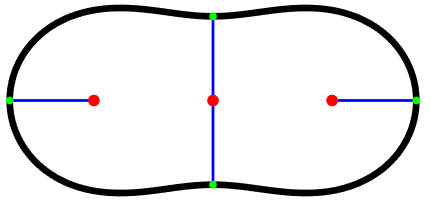
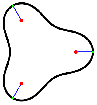
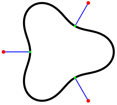
(a)		(b)		(c)

Figure 6: Reach attaining points for the Cassini oval with (a) 2 foci and (b) 3 foci. (c) Critical points arising from the algebraic closure of the reach for the Cassini oval with 3 foci.

Example 3.8.

The medial axis of the unit circle defined by $x_{1}^{2}+x_{2}^{2}=1$ is the origin and thus the reach of $1$ is attained at the origin. However, this reach attaining point is not isolated with respect to the critical reach correspondence since there are infinitely-many points on the unit circle where the reach is attained. Hence, the corresponding points computed via homotopy continuation need not be real. For example, using a multihomogeneous homotopy, $1$ is the unique positive critical value arising from $78$ distinct endpoints, none of which correspond with real points on the unit circle. Since $1$ is the only positive critical value, it is the reach.

Example 3.9.

The medial axis of the union of two concentric circles defined by

$$(x_{1}^{2}+x_{2}^{2}-1)(x_{1}^{2}+x_{2}^{2}-9)=0$$

is the union of the origin and the circle centered at the origin of radius $2$. Thus, the reach is $1$ which is attained at every point on the medial axis as shown in Figure 7. For example, using a multihomogeneous homotopy, the minimum positive critical value is $1$ which arises from 184 distinct endpoints. Of these, 168 correspond with the origin while the other 16 correspond with distinct points in $\mathbb{C}^{2}$ satisfying $x_{1}^{2}+x_{2}^{2}=4$. From (2), this one homotopy shows that the reach is at least $1$. For this example, it is easy to verify that there exist real critical points that yield a critical value of $1$ which shows that the reach is indeed equal to $1$.

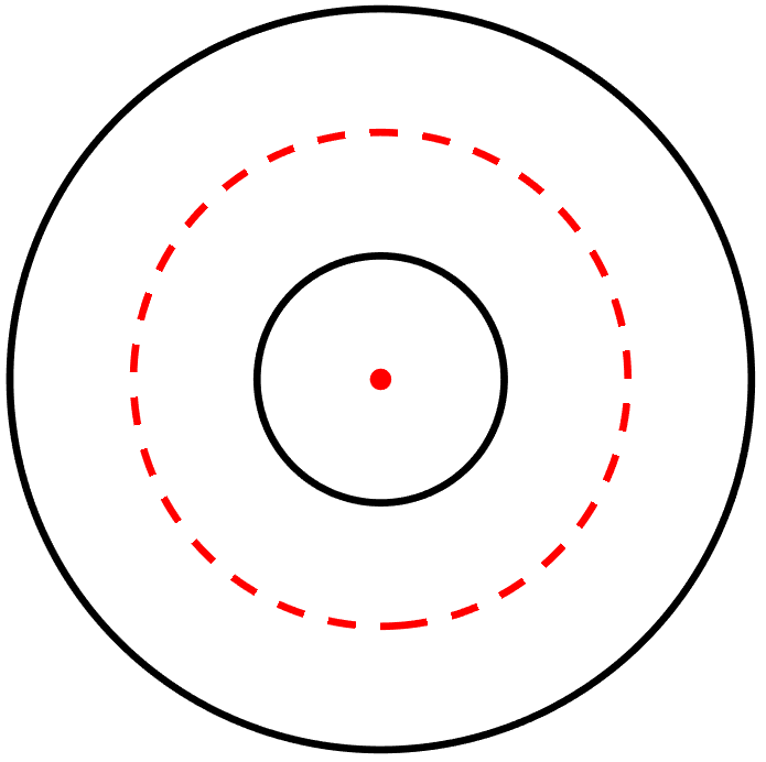
Figure 7: Reach obtained on a curve and a point for two concentric circles

4 Bottlenecks and weak feature size

The following expands upon the definition of geometric bottlenecks from Definition 2.3 and considers successive approximations of the weak feature size using higher order bottlenecks.

Definition 4.1.

Let $X$ be a compact subset of $\mathbb{R}^{n}$. A geometric bottleneck $z$ in $\operatorname{crit}(d_{X})$ has order $k\geq 2$ if $z$ is a convex combination of $k$ affinely independent points in $\pi_{X}(z)$ and is not a convex combination of any fewer number of points in $\pi_{X}(z)$. We will often refer to such a point $z$ as a geometric k-bottleneck of $X$.

Remark 4.2.

Definition 4.1 resembles a generalization of the index of critical points of a Morse function introduced by Gershokovich and Rubinstein [42]. The treatment by Bobrowski and Adler renders this connection clearer for distance functions [14, Def. 2.1], albeit for the case where $X$ is a finite point set. A geometric $k$-bottleneck of $X$ is a critical point of $d_{X}$ with index $k-1$ using that terminology. When $X$ is a finite set of points, this notion of index yields a decomposition similar to the classic cellular decomposition theorem of Morse theory (see, e.g., [58, Thm. 3.5] and [14, §4.2]). This does not extend to the case when $X$ is not finite. In particular, the Cassini oval with 2 foci in Example 2.4 and the unit circle in Example 3.8 are both counter examples. We use the term order rather than index to clarify that a Morse-type result does not apply in our setting.

Before considering the algebraic setting, the following highlights the relationship between geometric $k$-bottlenecks and weak feature size from Definition 2.3.

Proposition 4.3.

If $X$ is a compact subset of $\mathbb{R}^{n}$, then every geometric bottleneck has order at most $n+1$ and

$${\rm wfs}(X)=\inf_{z\text{ geom. }k\text{-bottleneck, }2\leq k\leq n+1}d_{X}(z).$$

Proof.

Suppose that $z$ is a geometric bottleneck of $X$. Then, by definition, $z$ is in the convex hull of $\pi_{X}(z)$. By Carathéodory’s Theorem [19], $z$ is a convex combination of at most $n+1$ points in $\pi_{X}(z)$ which shows that the order of $z$ is at most $n+1$. ∎

Remark 4.4.

From Proposition 4.3, it is natural to ask, for algebraic manifolds, if one must use all possible orders of geometric bottlenecks to determine the weak feature size or if one could use less, e.g., use only geometric $2$-bottlenecks. The Cassini oval with 3 foci in Example 2.4 lies in $\mathbb{R}^{2}$ and has no geometric $2$-bottlenecks. In particular, the weak feature size is attained at the origin, which is a geometric bottleneck of maximal order $3$. Similar Cassini oval constructions generalize to higher dimensions and also generalize [34, Ex 3.4].

Following a similar approach as in Section 3, one can relax the conditions of a geometric $k$-bottleneck to obtain algebraic conditions amenable to computational algebraic geometry over $\mathbb{C}$. As before, we assume that $X=V(F)\cap\mathbb{R}^{n}$ is nonempty and compact where $F$ is a polynomial system with real coefficients.

Definition 4.5.

Let $F=\{f_{1},\dots,f_{m}\}$ be a system of polynomials in $n$ variables with real coefficients such that $V(F)$ is equidimensional and smooth of codimension $c$ and $k\geq 2$. The $k^{\rm th}$ bottleneck correspondence of $F$, denoted $B_{k}(F)$, is

$$\left\{(x_{1},\dots,x_{k},t_{1},\dots,t_{k})\in\left(\mathbb{C}^{n}\right)^{k}\times\mathbb{C}^{k}~{}\left|\begin{array}[]{l}\begin{array}[]{l}\sum_{i=1}^{k}t_{i}=1,\end{array}\\ \begin{array}[]{l}z=\sum_{i=1}^{k}t_{i}x_{i},\end{array}\\ \begin{array}[]{l}d(x_{1},z)^{2}=d(x_{j},z)^{2}\ \text{ for }j=2,\dots,k\end{array}\\ \begin{array}[]{ll}F(x_{i})=0&\hbox{\multirowsetup\text{ for } $i=1,\dots,k$.}\\ \text{rank}[x_{i}-z\ JF(x_{i})^{T}]\leq c\end{array}\end{array}\right\}\right..$$

Let $\Gamma_{k}\subset\left(\mathbb{C}^{n}\right)^{k}\times\mathbb{C}^{k}$ consist of all points $(x_{1},\dots,x_{k},t_{1},\dots,t_{k})$ where any $t_{i}$ is $0$ or the set $\{x_{1},\dots,x_{k}\}$ is affinely dependent. Consider the map $\rho_{k}:\left(\mathbb{C}^{n}\right)^{k}\times\mathbb{C}^{k}\to\mathbb{C}^{n}$ defined by $\rho_{k}(x_{1},\dots,x_{k},t_{1},\dots,t_{k})=\sum_{i=1}^{k}t_{i}x_{i}$. A point $z\in\mathbb{C}^{n}$ is an algebraic $k$-bottleneck of $V(F)$ if $z\in\rho_{k}(B_{k}(F)\setminus\Gamma_{k})$. A real algebraic $k$-bottleneck of $V(F)$ is a point in $\mathbb{R}^{n}$ which is an algebraic $k$-bottleneck. Let $X=V(F)\cap\mathbb{R}^{n}$ and $R_{X,k}=X^{k}\times(0,1)^{k}\subset\left(\mathbb{R}^{n}\right)^{k}\times\mathbb{R}^{k}$. A real algebraic $k$-bottleneck of $X$ is a point in $\mathbb{R}^{n}$ in the image of $\rho_{k}((B_{k}(F)\cap R_{X,k})\setminus\Gamma_{k})$.

Remark 4.6.

Following the notation of Definition 4.5, every geometric $k$-bottleneck of $X$ is a real algebraic $k$-bottleneck of $X$. In particular, one has the following relationship:

$$\begin{array}[]{c}{\small\{\text{geometric $k$-bottlenecks of }X\}\subseteq\{\text{real algebraic $k$-bottlenecks of }X\}\subseteq}\\ {\small\{\text{real algebraic $k$-bottlenecks of }V(F)\}\subseteq\{\text{algebraic $k$-bottlenecks of }V(F)\}=\rho(B_{k}(F)\setminus\Gamma_{k}).}\end{array}$$

Typically, these inclusions are strict as the examples in Section 5 exhibit. In particular, for the second inclusion, it is possible for the image of $\rho_{k}$ to be real for nonreal input.

Example 4.7.

Consider computing the algebraic $2$-bottlenecks for the perturbed ellipsoid $X\subseteq\mathbb{R}^{2}$ from the Introduction defined by $F=x_{1}^{2}+x_{2}^{2}+x_{3}^{2}/2+x_{1}x_{3}/7-1$. The set $B_{2}(F)\setminus\Gamma_{2}$ consists of three points up to symmetry, which are depicted in Figure 3 with the black segments corresponding to the geometric $2$-bottleneck of $X$ while the blue segments correspond with real algebraic $2$-bottlenecks of $X$ that are not geometric $2$-bottlenecks of $X$.

4.1 Critical values

The following exhibits a result similar to Theorem 3.5.

Theorem 4.8.

Let $F$ be a polynomial system such that $V(F)$ is smooth and equidimensional of codimension $c$. Let $k\geq 2$ and $D_{k}:B_{k}(F)\to\mathbb{C}$ be defined by

$$(x_{1},\dots,x_{k},t_{1},\dots,t_{k})\mapsto\frac{1}{k}\sum_{i=1}^{k}d\left(x_{i},\rho_{k}(x_{1},\dots,x_{k},t_{1},\dots,t_{k})\right)^{2}.$$

Then, $D_{k}$ is constant on every connected component of $B_{k}(F)\setminus\Gamma_{k}$.

Proof.

Similarly to Theorem 3.5, it suffices to show constancy for an irreducible component $C$ not contained in $B_{k}(F)\setminus\Gamma_{k}$.

The following shows that every point in $B_{k}(F)\setminus\Gamma_{k}$ is a critical point of $D_{k}$. Since $D_{k}|_{C}$ is an algebraic map of irreducible quasiprojective algebraic sets, it follows by the algebraic version of Sard’s Theorem, e.g., [67, Thm A.4.10], that $D_{k}$ is not dominant, and therefore $D_{k}(C)$ is a single point because otherwise $C$ is not irreducible. Note that the critical points of $D_{k}$ are the same as those of $k\cdot D_{k}$ so we will consider $k\cdot D_{k}$ for simplicity.

Let $A_{k}(F)\subset\left(\mathbb{C}^{n}\right)^{k}\times\mathbb{C}^{n}$ be the set of $(x_{1},\dots,x_{k},z)$ satisfying

$$\begin{array}[]{l}F(x_{i})=0\ \text{ for }i=1,\dots,k,\\ d(x_{1},z)^{2}=d(x_{j},z)^{2}\ \text{ for }2\leq j\leq k.\end{array}$$

Clearly, there is an inclusion map $i:B_{k}(F)\to A_{k}(F)$ given by

$$(x_{1},\dots,x_{k},t_{1},\dots,t_{k})\mapsto\left(x_{1},\dots,x_{k},\sum_{i=1}^{k}t_{i}x_{i}\right).$$

By the chain rule, we need only prove that any point in the image of $i$ is a critical point of the map $D_{k}^{\prime}:A_{k}(F)\to\mathbb{C}$ defined by $(x_{1},x_{2},\dots,x_{k},z)\mapsto\sum_{i=1}^{k}d(x_{i},z)^{2}$. Since $V(F)$ is smooth and equidimensional, one may check directly that $A_{k}(F)$ has codimension $kc+k-1$. By elementary row operations, one reduces the problem to showing that $(x_{1},\dots,x_{k},z)$ is a critical point of $D_{k}^{\prime}$ if the $(km+k)\times(kn+n)$ matrix

$$\begin{pmatrix}JF(x_{1})&0&0&0&0&\dots&0\\ 0&JF(x_{2})&0&0&0&\dots&0\\ &&&\vdots&&&\\ 0&0&0&\dots&0&JF(x_{k})&0\\ 0&-(x_{2}-z)^{T}&0&\dots&0&0&(x_{2}-x_{1})^{T}\\ 0&0&-(x_{3}-z)^{T}&0&\dots&0&(x_{3}-x_{1})^{T}\\ &&&\vdots&&&\\ 0&0&0&\dots&0&-(x_{k}-z)^{T}&(x_{k}-x_{1})^{T}\\ (x_{1}-z)^{T}&0&0&0&\dots&0&(z-x_{1})^{T}\end{pmatrix}$$

has rank at most $kc+k-1$ where $m$ is the number of polynomials in $F$. Suppose that $(x_{1},\dots,x_{k},z)$ is in the image of the inclusion map $i$. Then, the first $kn$ columns of this matrix contribute at most $kc$ to the dimension of the column space and the final $n$ columns contribute at most by $k-1$ since $x_{2}-x_{1},\dots,x_{k}-x_{1}$ span the affine hull of $x_{1},\dots,x_{k}$ and $z-x_{1}$ is in that affine hull. Altogether the rank of the matrix is at most $kc+k-1$. ∎

Remark 4.9.

For $k=2$, this proof shows that the algebraic $2$-bottlenecks of $V(F)$ correspond with a subset of the Zariski closure $C(F)\setminus\Delta$ where $C(F)$ is the critical reach correspondence. In contrast to $C(F)$, however, the correspondence $B_{2}(F)$ does not contain functions corresponding to the gradients of $\operatorname{rank}$ conditions. This is illustrated in Figure 6(a) for the Cassini oval with $2$ foci.

As with Theorem 3.5 yielding Corollary 3.6, Theorem 4.8 provides the following.

Corollary 4.10.

Let $F$ be a polynomial system in $n$ variables with real coefficients such that $V(F)$ is smooth and equidimensional of codimension $c$ and $X=V(F)\cap\mathbb{R}^{n}$ is nonempty and compact. For each $k=2,\dots,n+1$, one can use a parameter homotopy [59] to compute a finite set of points $E_{k}$ which contains at least one point in each connected component of $B_{k}(F)\setminus\Gamma_{k}$. Then,

$$0<\min_{k=2,\dots,n+1}\left(\min_{e\in E_{k}\text{~{}with~{}}D_{k}(e)>0}\sqrt{D_{k}(e)}\right)\leq\operatorname{wfs}(X).$$ (4)

Remark 4.11.

As with Corollary 3.6, an additional reality test, e.g., [49], can be used to determine the weak feature size. When $\bigcup_{k=2}^{n}\left(B_{k}(F)\setminus\Gamma_{k}\right)$ is finite, reality testing simply decides the reality of each critical point.

Remark 4.12.

Compactness may be removed as a requirement in Theorem 4.8 and Corollary 4.10, but some care is necessary when $X=V(F)\cap\mathbb{R}^{n}$ is not compact. As an illustration, consider $F=x^{2}y^{2}-1$ with $X$ shown in Figure 8. Then, Theorem 4.8 shows that the weak feature size of $X=V(F)\cap\mathbb{R}^{2}$ inside any closed Euclidean ball of finite radius centered at the origin that intersects $X$ in $\mathbb{R}^{2}$ must be positive. By an explicit computation, one can see that the only contributors to the weak feature size in $B_{2}(F)\setminus\Gamma_{2}$ are isolated solutions as shown in Figure 8. The subtlety is that the manifold $V(F)\cap\mathbb{R}^{2}$ is not homotopy equivalent to any of its thickenings and thus it is not an absolute neighborhood retract. Therefore, Theorem 2.5 does not apply.

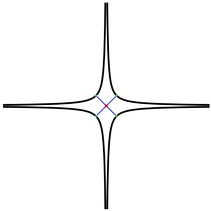
Figure 8: Real solutions of $x^{2}y^{2}=1$ with its geometric bottlenecks

Example 4.13.

Consider the ellipsoid $X\subseteq\mathbb{R}^{2}$ defined by $F=x_{1}^{2}+x_{2}^{2}+x_{3}^{2}/2-1$ from the Introduction that is depicted in Figure 2. We consider computing the algebraic $2$-bottlenecks using Corollary 4.10 in two different ways: using a parameter homotopy in the corresponding space of multihomogeneous systems and using a parameter homotopy from the perturbed ellipsoid computed in Example 4.7.

For the first approach, one obtains $6$ points in $B_{2}(F)\setminus\Gamma_{2}$. Two of these points are real and equal up to symmetry. They correspond with the blue segments connecting the magenta points in Figure 2 at a distance of $\sqrt{2}$ from the origin, i.e., $D_{2}=2$. The other 4 points are nonreal and have $D_{2}=1$. These lie on a positive-dimensional component arising from antipodal points on the unit circle in the $(x_{1},x_{2})$-plane whose real points are shown in Figure 2. For this example, it is easy to verify that there exist real points on this component which are also geometric $2$-bottlenecks.

For the second approach, we can consider the family of algebraic $2$-bottlenecks for

$$F_{t}=x_{1}^{2}+x_{2}^{2}+x_{3}^{2}/2+tx_{1}x_{2}-1.$$

Example 4.7 shows that, at the generic parameter value $t=1/7$, $V(F_{t})$ has three algebraic $2$-bottlenecks. We then used a parameter homotopy to track these three solutions along the sufficiently general path defined by

$$t(s)=\frac{1}{7}\cdot\frac{\gamma s}{1-s+\gamma s}\text{~{}~{}where~{}~{}}\gamma=2+3\sqrt{-1}$$

as $s$ goes from $1$ to $0$. This yielded three real solutions which lie along the three coordinate axes. The two lying along the $x_{1}$ and $x_{2}$ coordinate axes have $D_{2}=1$ while the third that lies along the $x_{3}$ coordinate axis has $D_{2}=2$.

4.2 Critical points

The remainder of this section considers the finiteness of algebraic $k$-bottlenecks for general complete intersections of codimension $c$ in $\mathbb{C}^{n}$. Of course, we naturally assume that $n\geq 1$ and $1\leq c\leq n$. Let $(d_{1},\dots,d_{c})\in\mathbb{N}^{c}$ and consider $P_{i}=\mathbb{P}^{N_{i}}$ where $N_{i}=\binom{d_{i}+n}{d_{i}}-1$ which is the parameter space of hypersurfaces in $\mathbb{C}^{n}$ of degree at most $d_{i}$. Furthermore, complete intersections in $\mathbb{C}^{n}$ of codimension $c$ and degree type $(d_{1},\dots,d_{c})$ are parameterized by an open subset $U\subseteq\prod_{i=1}^{c}P_{i}$. Let $X_{u}$ denote the complete intersection in $\mathbb{C}^{n}$ corresponding to $u\in U$ and $F_{u}$ be the system of $c$ polynomials in $n$ variables that defines $X_{u}$.

Definition 4.14.

For $k\geq 2$, the k-bottleneck correspondence for degree pattern $(d_{1},\dots,d_{c})$, denoted $S_{k}$, is the set of points $(u,x_{1},\dots,x_{k},t_{1},\dots,t_{k})\in U\times\left(\mathbb{C}^{n}\right)^{k}\times\mathbb{C}^{k}$ such that

$$(x_{1},\dots,x_{k},t_{1},\dots,t_{k})\in B_{k}(F_{u}).$$

We will analyze $S_{k}$ via projections onto its factors. In particular, let $\pi:S_{k}\to\left(\mathbb{C}^{n}\right)^{k}\times\mathbb{C}^{k}$ and $\eta:S_{k}\to U$ be the projection maps. For any $u\in U$, the fiber $\eta^{-1}(u)$ is $\{u\}\times B_{k}(F_{u})$.

The following provides a finiteness condition for algebraic $k$-bottlenecks. Since geometric $k$-bottlenecks are algebraic $k$-bottlenecks, this immediately implies a finiteness condition for geometric $k$-bottlenecks as well.

Theorem 4.15.

Let $k\geq 2$ and $(d_{1},\ldots,d_{c})\in\mathbb{N}^{c}$ such that each $d_{i}\neq 2$. For general $u\in U$, the set of algebraic $k$-bottlenecks for $V(F_{u})$ is finite. In particular, for general $u\in U$, $\eta^{-1}(u)\setminus\Gamma_{k}$ is finite.

The proof of this theorem is provided at the end of this section and follows from the Alexander-Hirschowitz Theorem [2], which is a result for homogeneous hypersurfaces. Thus, we need to move from affine space to projective space. In particular, $\mathbb{P}^{N}$ parameterizes homogeneous polynomials in $n+1$ variables of degree $d$ where $N=\binom{d+n}{d}-1$. For $a\in\mathbb{P}^{N}$, let $F_{a}(x_{0},\ldots,x_{n})$ denote the corresponding homogeneous polynomial of degree $d$.

Let $p_{1},\ldots,p_{k}\in\mathbb{P}^{n}$ be general. The Alexander-Hirschowitz Theorem considers the dimension of the interpolation space of polynomials of degree $d$ having at least a double point at $p_{i}$, namely

$$I_{n,k}=\left\{a\in\mathbb{P}^{N}~{}\left|~{}F_{a}(p_{i})=\frac{\partial F_{a}}{\partial x_{j}}(p_{i})=0\text{ for }j=1,\dots,n\text{ and }i=1,\dots,k\right\}\right..$$

Theorem 4.16 (Alexander-Hirschowitz [2]).

The interpolation space $I_{n,k}$ has the expected dimension, i.e., $\dim(I_{n,k})=\min\{(n+1)k,N\}$, except for the following cases

• $d=2,2\leq k\leq n$;

• $n=2,d=4,k=5$;

• $n=3,d=4,k=9$;

• $n=4,d=3,k=7$;

• $n=4,d=4,k=14$.

An equivalent statement of this theorem is that the $k$-secant variety of the $d^{\rm th}$ Veronese embedding of $\mathbb{P}^{n}$, which we will call the $(n,d)$-Veronese variety $V_{n,d}$, has the expected dimension except for the listed exceptions.

Remark 4.17.

Suppose that $p_{1},\dots,p_{k},q_{1},\dots,q_{k}\in\mathbb{P}^{n}$ where $k\leq n+1$ are such that $p_{1},\dots,p_{k}$ and $q_{1},\dots,q_{k}$ each span a $(k-1)$-dimensional space. Let $I_{p}$ and $I_{q}$ denote the interpolation space $I_{n,k}\subseteq\mathbb{P}^{N}$ as defined above, respectively. Then, $I_{p}$ and $I_{q}$ have the same dimension. To see this, first note that there is a full rank linear map $L:\mathbb{P}^{n}\rightarrow\mathbb{P}^{n}$ such that $Lq_{i}=p_{i}$ for all $i$. More explicitly, complete $p_{1},\dots,p_{k}$ to a spanning set $p_{1},\dots,p_{n+1}$ of $\mathbb{P}^{n}$ and similarly for $q_{1},\dots,q_{k}$. Let $P=(p_{1}\cdots p_{n+1})$ and $Q=(q_{1}\cdots q_{n+1})$ be $(n+1)\times(n+1)$-matrices whose columns are the homogeneous coordinates of $p_{1},\dots,p_{n+1}$ and $q_{1},\dots,q_{n+1}$. Then $L$ is represented by $PQ^{-1}$.

The group $\textrm{PGL}_{n}$ acts on the parameter space of hyper surfaces $\mathbb{P}^{N}$ as follows: for $T\in\textrm{PGL}_{n}$, $Ta$ is given by the polynomial $F_{a}\circ T^{-1}$. Using this action and with $L$ as above, $LI_{q}=I_{p}$. In particular, by the chain rule $J(F_{a}\circ L)(q_{i})=JF_{a}(p_{i})L$ for all $i$ and $a\in\mathbb{P}^{N}$.

Proposition 4.18.

Let $p_{1},\ldots,p_{k}\in\mathbb{P}^{n}$ with $k\leq n+1$ and suppose that $p_{1},\ldots,p_{k}$ span a $(k-1)$-dimensional subspace of $\mathbb{P}^{n}$. With notation as above, the interpolation space has the expected dimension except if $d=2$ and $2\leq k\leq n$.

Proof.

Assume that $d>2$ or that $k$ is not in $[2,n]$. Let $q_{1},\dots,q_{k}\in\mathbb{P}^{n}$ be independent points such that their interpolation space has the expected dimension (this is true for general $q_{1},\dots,q_{k}$ by the Alexander-Hirschowitz theorem). Let $L:\mathbb{P}^{n}\rightarrow\mathbb{P}^{n}$ be a full rank linear map such that $Lq_{i}=p_{i}$ for all $i$ and let $I_{p}$ and $I_{q}$ be the interpolation spaces of $p_{1},\dots,p_{k}$ and $q_{1},\dots,q_{k}$, respectively. Since $I_{p}=LI_{q}$, they have the same dimension. ∎

Proposition 4.19.

If the $k$-secant variety of the $(n,d)$-Veronese variety $V_{n,d}$ has the expected dimension for generic $p_{1},\ldots,p_{k}\in\mathbb{P}^{n}$, then the $k(n+1)$ linear forms in $(a_{0},\dots,a_{N})$ which comprise the entries of $JF_{a}(p_{1}),\ldots,JF_{a}(p_{k})$ are independent.

Proof.

Let $\nu(p)=\nu_{d,n}(p)=(p^{j})_{\{j\}}\in V_{n,d}$. Then, the projective tangent space to $V_{n,d}$ at $\nu(p)$ is spanned by $\nu_{x_{0}}(p),\ldots,\nu_{x_{n}}(p)$ where $\nu_{x_{i}}=\frac{\partial\nu}{\partial x_{i}}$. The coefficients of the linear form $\frac{\partial F_{a}}{\partial x_{i}}(p)$ are the elements of the $(N+1)$-vector $\nu_{x_{i}}(p)$. ∎

If $c=n$, the complete intersection $X_{u}$ itself is finite and Theorem 4.15 is immediate, so assume that $c<n$. We may reduce to the case where none of the equations defining $X_{u}$ are linear, that is $d_{i}>2$ for all $i$. Indeed, for a generic hyperplane $H\subseteq\mathbb{C}^{n}$ there is a linear map which preserves algebraic $k$-bottlenecks of $X_{u}$ while eliminating a variable. After repeatedly removing linear equations we may assume that $d_{i}>2$ for all $i$.

In order to show that a general complete intersection has a finite number of algebraic $k$-bottlenecks, we need to show that the generic fiber of the projection $\eta:S_{k}\to U$ is finite. We do this by first studying the dimension of the fibers of the projection $\pi:S_{k}\to(\prod_{i=1}^{k}\mathbb{C}^{n})\times\mathbb{C}^{k}$.

Lemma 4.20.

Let $(x_{1},\dots,x_{k},t_{1},\dots,t_{k})$ be an element in the image $\pi(S_{k})\setminus\Gamma_{k}$. Then, $\pi^{-1}(x_{1},\dots,x_{k},t_{1},\dots,t_{k})$ has codimension $kn$ in $U$.

Proof.

By assumption, the equations

$$\sum_{i=1}^{k}t_{i}=1,\ \ z=\sum_{i=1}^{k}t_{i}x_{i},\ \ d(x_{1},z)^{2}=d(x_{j},z)^{2},\ \ 2\leq j\leq k$$

are satisfied. The fiber $\pi^{-1}(x_{1},\dots,x_{k},t_{1},\dots,t_{k})$ is the algebraic subset of $U$ defined by the conditions

$$x_{i}\in X_{u}\ \text{ and }\ \text{rank}[x_{i}-z\ JF_{u}(x_{i})^{T}]\leq c\ \text{ for }1\leq i\leq k\text{.}$$

First note that $x_{i}-z=\sum_{j=1,j\not=i}^{k}t_{j}(x_{i}-x_{j})$ for all $i$. In particular, $x_{i}-z$ is not $0$ because $\{x_{i}-x_{j}\}_{j=1,j\not=i}^{k}$ is linearly independent by assumption and none of $t_{1},\dots,t_{k}$ is $0$. For all $i$, there subsequently exists a full rank $n\times n$ matrix $M_{i}$ such that $M_{i}(x_{i}-z)$ is $e_{1}$, the standard basis vector for $\mathbb{C}^{n}$. The fiber is equivalently defined by the conditions

$$F_{u}(x_{i})=0\ \text{ and }\ \text{rank}\begin{bmatrix}1&0&\dots&0\\ 0&&&\\ \vdots&&(M_{i}(JF_{u}(x_{i})^{T}))^{\prime}\\ 0&&\end{bmatrix}\leq c\ \text{ for }1\leq i\leq k$$

where for any matrix $M$, $M^{\prime}$ denotes $M$ with the first row deleted.

We claim that the collection of forms in $u$ comprising the entries of $F_{u}(x_{i})$ and $JF_{u}(x_{i})$ across all $i$, $1\leq i\leq k$, is independent. Forms arising from different components of $F_{u}$ involve disjoint subsets of the coefficients in $u$, so it suffices to consider the case where $F_{u}$ is a single polynomial $f$ of degree $d>2$. Let $\overline{f}$ denote the homogenization of $f$ and $\overline{x_{i}}$ denote the point in $\mathbb{P}^{n}$ with projective coordinates $[x_{i};1]$. Note that since the vectors $x_{1},\dots,x_{k}$ are affinely independent, the points $\overline{x_{1}},\dots,\overline{x_{k}}$ span a $(k-1)$-dimensional subspace of $\mathbb{P}^{n}$ as in the statement of Proposition 4.18. Suppose to the contrary that a relation of the form $\sum_{i=1}^{k}\alpha_{i}f(x_{i})=\sum_{1\leq i\leq k,1\leq j\leq n}\beta_{ij}\frac{\partial f}{\partial y_{j}}(x_{i})$ holds. Then the same relation holds substituting $\overline{f}$ for $f$ and $\overline{x_{i}}$ for $x_{i}$. By Euler’s formula, $d\overline{f}(\overline{x_{i}})=\sum_{j=1}^{n+1}(\overline{x_{i}})_{j}\frac{\partial\overline{f}}{\partial y_{j}}(\overline{x_{i}})$. So we obtain a relation which contradicts Propositions 4.18 and 4.19.

We see that $\pi^{-1}(x_{1},\dots,x_{k},t_{1},\dots,t_{k})$ is a proper intersection of $k$ determinantal varieties which, by standard results, have codimension $n-c$ and a linear space defined by the linear forms $F_{u}(x_{i})$ for $1\leq i\leq k$. Altogether, the codimension of the fiber is $k(n-c+c)=kn$. ∎

Lemma 4.21.

The dimension of $S_{k}\setminus\pi^{-1}(\Gamma_{k})$ is the dimension of $U$.

Proof.

Consider the image $V$ of $\pi:(S_{k}\setminus\pi^{-1}(\Gamma_{k}))\to(\prod_{i=1}^{k}\mathbb{C}^{n})\times\mathbb{C}^{k}$. One can easily see that the image is the open algebraic subset comprised of all $(x_{1},\dots,x_{k},t_{1},\dots,t_{k})$ where

$$\sum_{i=1}^{k}t_{i}=1,\ \ z=\sum_{i=1}^{k}t_{i}x_{i},\ \ d(x_{1},z)^{2}=d(x_{j},z)^{2},\ \ 2\leq j\leq k,$$

the $x_{1},\dots,x_{k}$ are affinely independent, and none of the $t_{i}$ are 0. We claim that the image has codimension $k$, i.e., dimension $kn$. In fact, the image $V$ is birationally equivalent to $\prod_{i=1}^{k}\mathbb{C}^{n}$. The forward morphism is given by the projection map $g:V\to\prod_{i=1}^{k}\mathbb{C}^{n}$ where $g(x_{1},\dots,x_{k},t_{1},\dots,t_{k})=(x_{1},\dots,x_{k})$. Setting $X$ to be the $n\times k$ matrix whose columns are the the vectors with coordinates $x_{1},\dots,x_{k}$, the inverse $h:\prod_{i=1}^{k}\mathbb{C}^{n}\to V$ is given by taking $h(x_{1},\dots,x_{k})$ to be $(x_{1},\dots,x_{k},t_{1}(X),t_{2}(X),\dots,t_{k}(X))$ where the functions $t_{i}(X)$ are rational functions yielding the barycentric coordinates of the circumcenter of the simplex whose vertices are the columns of $X$ (see, e.g., [40, Thm. 2.1.1] and [68, pp. 707–708]).

By Lemma 4.20, the fiber of $\pi$ has codimension $kn$ for $z$ in the image $V$. It follows that $S_{k}\setminus\pi^{-1}(\Gamma_{k})$ has dimension $\dim(U)-kn+(kn+k-k)=\dim(U)$. ∎

Building on these results, we now present the proof of Theorem 4.15.

Proof of Theorem 4.15.

Let $S$ be an irreducible component of $S_{k}\setminus\pi^{-1}(\Gamma_{k})$. By Lemma 4.21, $\dim{S}\leq\dim{U}$. If $\eta_{|S}$ does not dominate $U$, then $S\cap\eta^{-1}(u)$ is empty for general $u\in U$. However, if $\eta_{|S}$ dominates $U$, then $\dim{S}=\dim{U}$ and $\eta^{-1}(u)$ is finite for general $u\in U$. ∎

5 Computational experiments for feature sizes

This Section contains results from computing the reach, bottlenecks, and weak feature size of examples of co-dimension $1$ in $\mathbb{R}^{2}$ and co-dimensions $1$ and $2$ in $\mathbb{R}^{3}$. Data results and code for reproducing these computations are available at https://github.com/P-Edwards/wfs-and-reach-examples.

Example 5.1.

Consider the “butterfly curve” in $\mathbb{R}^{2}$, which is the real part of the algebraic variety defined as $V(F)\cap\mathbb{R}^{2}$ where $F=x^{4}-x^{2}y^{2}+y^{4}-4x^{2}-2y^{2}-x-4y+1$. This example has been considered before, e.g., by Brandt and Weinstein [15].

The algebraic medial axis for the butterfly curve was computed using numerical algebraic geometry and found to be irreducible of degree $120$. The real part of this curve is shown in Figure 9(a) with the pieces in cyan forming the geometric medial axis. A lower bound of $0.103$ on the reach was estimated with a homotopy continuation method based on Corollary 3.6 in agreement with [15, Ex. 6.1]. The points computed via Corollary 3.6 on the geometric medial axis are shown in red in Figure 9(b).

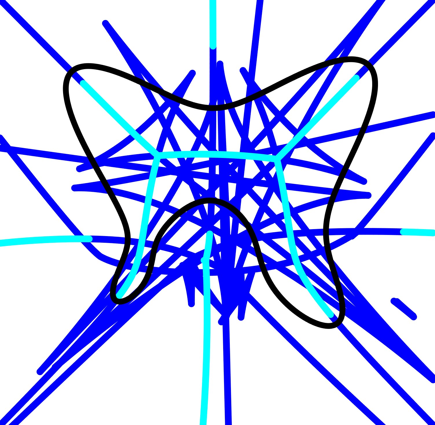
(a)	(b)

Figure 9: For butterfly curve: (a) algebraic and geometric medial axis; (b) geometric medial axis with critical points.

To compute the weak feature size of $V(F)\cap\mathbb{R}^{2}$, we used the numerical algebraic geometric method in Corollary 4.10. For both $k=2$ and $k=3$, the results indicate that the irreducible components of $B_{k}(F)$ not contained in $\Gamma_{k}$ are all isolated points, i.e., $V(F)$ has finitely many algebraic bottlenecks. The following table provides a summary of the outputs. In particular, the weak feature size of $V(F)\cap\mathbb{R}^{2}$ was determined to be approximately 0.251 and is attained by a geometric 2-bottleneck (cf., [15, Ex. 6.1]). Figures 10 and 11 show various types of bottlenecks for the butterfly curve.

	$k=2$	$k=3$
Number of points on $B_{k}(G)$ computed	392	2817
Number of computed points in $\Gamma_{k}$	200	1089
Algebraic $k$-bottlenecks of $V(G)$	96	288
Real algebraic $k$-bottlenecks of $V(G)$	26	28
Real algebraic $k$-bottlenecks of $V(G)\cap\mathbb{R}^{2}$	22	17
Geometric $k$-bottlenecks of $V(G)\cap\mathbb{R}^{2}$	3	2

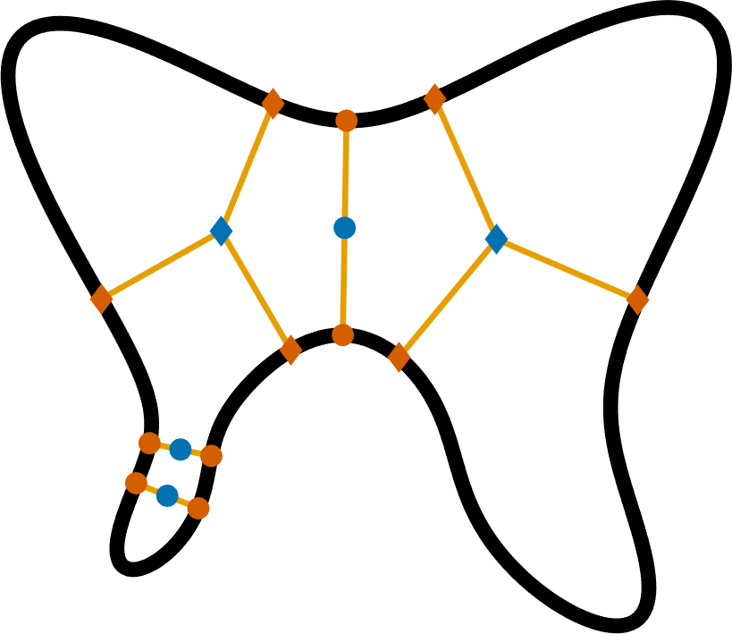
Figure 10: Geometric 2-bottlenecks (dark blue circles) and 3-bottlenecks (dark blue diamonds) of the butterfly curve. Orange dots are distance minimizers and connect to bottlenecks with light orange lines.

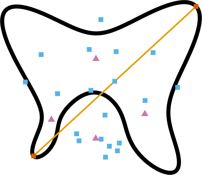
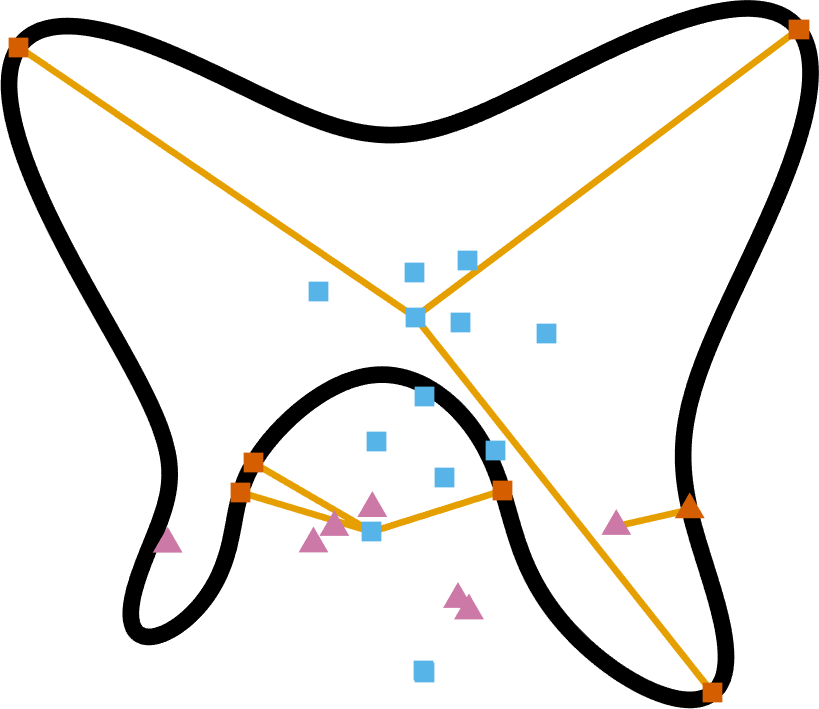
Figure 11: Algebraic 2-bottlenecks (left) and 3-bottlenecks (right) of the butterfly curve. Algebraic bottlenecks are blue and real algebraic bottlenecks of the butterfly curve are pink. For an illustrative subset, orange distance-critical points are connected to their corresponding bottleneck by orange lines.

Example 5.2.

As an example of a non-quadratic complete intersection where Theorem 4.15 holds, consider the intersection of a torus and Clebsch surface in $\mathbb{R}^{3}$ defined by

$$F=\left[\begin{array}[]{c}(R^{2}-r^{2}+x^{2}+y^{2}+z^{2})^{2}-4R^{2}(x^{2}+y^{2})\\ x^{3}+y^{3}+z^{3}+1-(x+y+z+1)^{3}\end{array}\right]$$

with $R=\frac{3}{2}$ and $r=1$. In particular, the second equation is an algebraic surface with all 27 exceptional lines contained in $\mathbb{R}^{3}$ [28]. This curve is illustrated in Figure 12.

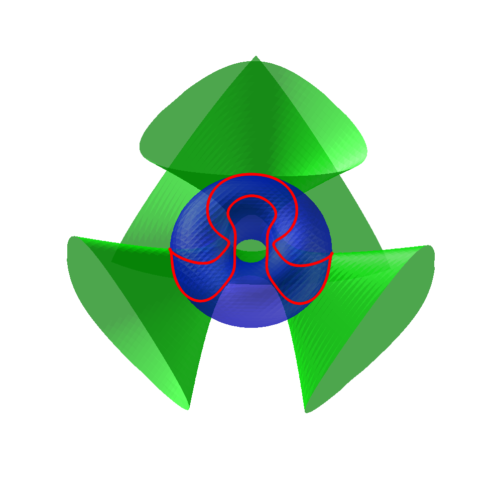
Figure 12: Curve (red) at the intersection of a torus (blue) and Clebsch surface (green).

We computed the the weak feature size for this curve by using homotopy continuation to compute $B_{k}(F)$ for $k=2,3,4$. The computations indicated that the irreducible components of $B_{k}(G)$ not contained in $\Gamma_{k}$ are all isolated points. The weak feature size is approximately 0.405, which is attained at a geometric 2-bottleneck. In particular, this example of computing the weak feature size is the most complicated we will consider in terms of computational cost. The cost of computing bottlenecks increases substantially with higher bottleneck order, both due to increasing the ambient dimension of $B_{k}(F)$ and because there are $k!$ solutions in $B_{k}(F)$ for each algebraic $k$-bottleneck. Regeneration methods [51] were used to make computations for this example more tractable. In particular, the 4-bottlenecks required approximately one week of computation on a 24-CPU computer. The table below summarizes the results.

	$k=2$	$k=3$	$k=4$
Number of points on $B_{k}(F)$ computed	2736	94548	1431936
Number of computed points in $\Gamma_{k}$	576	2424	0
Algebraic $k$-bottlenecks of $V(F)$	1080	15354	59664
Real algebraic $k$-bottlenecks of $V(F)$	68	324	586
Real algebraic $k$-bottlenecks of $V(F)\cap\mathbb{R}^{3}$	50	134	86
Geometric $k$-bottlenecks of $V(F)\cap\mathbb{R}^{3}$	22	6	0

Example 5.3.

We conclude this collection of examples with the quartic surface in $\mathbb{R}^{3}$ from [36, §5.2] illustrated in Figure 13 and defined by

$$F=4x^{4}+7y^{4}+3z^{4}-3-8x^{3}+2x^{2}y-4x^{2}-8xy^{2}-5xy+8x-6y^{3}+8y^{2}+4y.$$

As in the previous examples, we computed that $V(F)$ has finitely many algebraic bottlenecks of orders $2$ and $3$. Since computing $4$-bottlenecks proved similarly expensive to Example 5.2, they were not computed for this example.

This surface exhibits interesting behavior from an algebraic viewpoint. A point $p$ approximated by $(0.458,-0.97,0)$ was computed to be the only geometric 2-bottleneck of $V(F)\cap\mathbb{R}^{3}$ as shown in Figure 13. The two corresponding points in $\rho_{2}^{-1}(p)\subseteq B_{2}(F)$ are isolated in the bottleneck correspondence but are singular, i.e., have multiplicity higher than 1. The weak feature size of approximately $0.354$ is attained at $p$ with Figure 13 also showing the two geometric 3-bottlenecks. The following table summarizes this computation.

	$k=2$	$k=3$
Number of points on $B_{k}(F)$ computed	2220	40672
Number of computed points in $\Gamma_{k}$	0	8191
Geometric $k$-bottlenecks of $V(F)\cap\mathbb{R}^{3}$	1	2

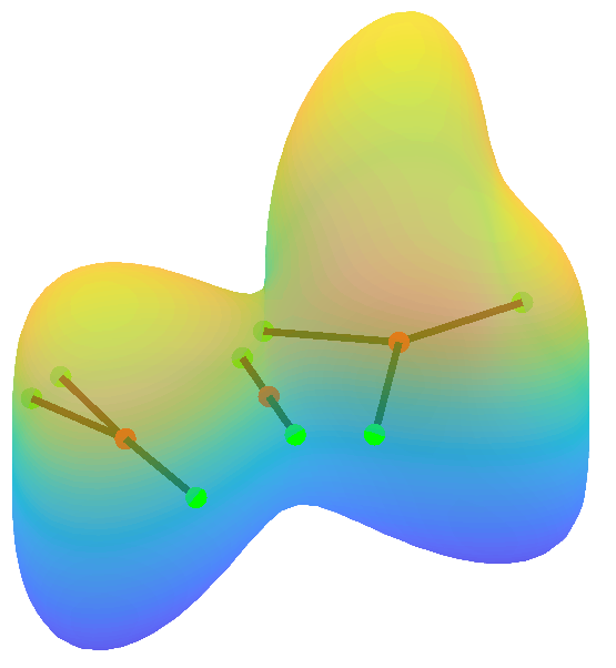
Figure 13: Quartic surface with geometric 2- and 3-bottlenecks

6 Persistent homology and adaptive sparsification

Memory requirements currently comprise the most serious practical limitation for computing persistent homology [63]. If $\hat{X}\subseteq\mathbb{R}^{n}$ is a finite point sample, the memory required to compute the persistence diagram for the persistence module $H_{\ell}R_{\hat{X}}$ rapidly increases with the number of points in $\hat{X}$. One strategy to mitigate this cost is to add a “subsampling” step before computing persistent homology. The aim is to remove points from a sample $\hat{X}$ using a procedure that does not substantially degrade output persistence diagrams. We can now compute both the weak feature size and local feature size of algebraic manifolds, which enables us to test algorithms on samples which fulfill theoretical density requirements. This section provides a proof-of-concept for how one can use our computational methods to test the behavior of geometric algorithms.

We will consider three subsampling procedures: a uniform subsampling approach and two “adaptive” approaches. The latter two are based on results of Dey et al. [32] and Chazal and Lieuter [26], and remove points from a sample of a space $X$ based on the local feature size of $X$. More points are retained in regions where the local feature size is lower, which is a proxy for retaining more points in regions of higher curvature as illustrated in Figure 14.

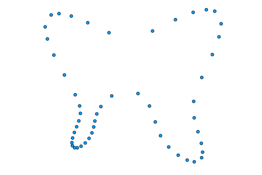
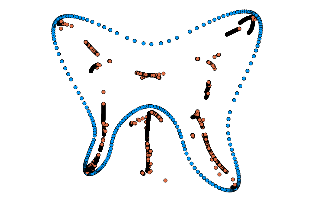
Figure 14: Adaptive samples (blue) of the butterfly curve from Example 5.1 with respect to $\operatorname{lfs}$ (left) and “lean feature size” (right). More points are retained closer to the medial axis and “lean medial axis” (orange) respectively.

6.1 Subsampling with functions

All three subsampling approaches we will consider fit into a greedy framework. Algorithm 2 summarizes this framework and follows the presentation of [32, Alg. 1].

1

Input : Sample $\hat{X}\subseteq\mathbb{R}^{n}$ and function $s:\hat{X}\to\mathbb{R}$

Output : A subsample of $\hat{X}$

2 Put $\hat{X}$ in a max priority queue sorted by $s$;

3 Set Output to $\emptyset$;

4 while The queue is not empty do

5       Add the highest priority $\hat{x}_{1}$ in the queue to Output and remove it from the queue;

6       Delete any point $\hat{x}_{2}$ from the queue where $\|\hat{x}_{1}-\hat{x}_{2}\|\leq s(\hat{x}_{1})$;

7      

8 end while

Return(Output)

Algorithm 2 Subsample

Example 6.1 (Uniform subsample).

Let $X=V(F)\cap\mathbb{R}^{n}$ where $V(F)$ is smooth and equidimensional. We can compute $\omega<\operatorname{wfs}(X)$ via homotopy continuation as we did in Section 5. For any $\lambda\in[0,1]$, define $\omega_{\lambda}:\mathbb{R}^{n}\to\mathbb{R}$ to be the constant function given by $\omega_{\lambda}(z)=\lambda\omega$. The output of $\textsc{Subsample}(\hat{X},\omega_{\lambda})$ is a “uniform subsample” of $\hat{X}$. If $\hat{X}$ is a $(\delta,\mu\omega)$-sample of $X$, then $\textsc{Subsample}(\hat{X},\omega_{\lambda})$ is a $(\delta,(\mu+\lambda)\omega)$-sample of $X$.

Example 6.2 (Local adaptive subsample).

With $X$ and $F$ as in the previous example and $\operatorname{lfs}$ being the local feature size function of $X$, for any $\lambda\in[0,1]$, define $\operatorname{lfs}_{\lambda}:\mathbb{R}^{n}\to\mathbb{R}_{\geq 0}$ by $\operatorname{lfs}_{\lambda}(z)=\lambda\operatorname{lfs}(z)$. The output of $\textsc{Subsample}(\hat{X},\operatorname{lfs}_{\lambda})$ is an “adaptive subsample” of $\hat{X}$ with respect to the local feature size. In practice, we compute $\widehat{\operatorname{lfs}}(z)\leq\operatorname{lfs}(z)$ for any $z\in\hat{X}$ via homotopy continuation as in Corollary 3.6.

Example 6.3 (Lean adaptive subsample).

Let $\hat{X}\subseteq\mathbb{R}^{n}$ be a point sample. In [32, Def. 3], Dey et al. define the $\frac{\pi}{5}$-lean set of $\hat{X}$, $L_{\frac{\pi}{5}}$, to be a subset of the set of midpoints $\{\frac{p+q}{2}\}_{p\not=q\in\hat{X}}$ that also fulfills other geometric conditions (see [32] for details). In particular, the $\frac{\pi}{5}$-lean set of $\hat{X}$ can be computed using just the points in $\hat{X}$ as input. They also show that, if $\hat{X}$ is a dense sample from a manifold in an appropriate sense, then the distance function $d_{L_{\frac{\pi}{5}}}$ estimates the distance to a subset of the medial axis of $X$. For $\lambda\in[0,1]$ define $\operatorname{lnfs}_{\lambda}:\mathbb{R}^{n}\to\mathbb{R}_{\geq 0}$ by $\operatorname{lnfs}_{\lambda}(z)=\lambda d_{L_{\frac{\pi}{5}}}(z)$. The output of $\textsc{Subsample}(\hat{X},\operatorname{lnfs}_{\lambda})$ is an adaptive subsample of $\hat{X}$ with respect to the lean feature size.

6.2 Adaptive Vietoris-Rips complexes

Standard Vietoris-Rips persistent homology is not appropriate when $\hat{X}$ is an adaptive subsample. Instead, we must use an adaptive Vietoris-Rips complex.

Definition 6.4.

Let $\hat{X}$ be a finite subset $\mathbb{R}^{n}$ and let $r:\hat{X}\to\mathbb{R}_{\geq 0}$. For any non-empty $\sigma\subseteq\hat{X}$, define $\operatorname{diam}_{r}(\sigma)=\max_{p,q\in\sigma}\frac{\|p-q\|}{r(p)+r(q)}$. Then, for $t\geq 0$, the $r$-adaptive Vietoris-Rips complex of $\hat{X}$ at threshold $t$ is the abstract simplicial complex

$$R_{\hat{X},r}(t):=\{\sigma\not=\emptyset\subseteq\hat{X}\mid\operatorname{diam}_{r}(\sigma)\leq t\}\text{.}$$

When $r$ is the constant function with output $1/2$, $R_{\hat{X},r}$ is the standard Vietoris-Rips complex. We will use $r=\operatorname{lfs}$ when $\hat{X}$ is an adaptive subsample with respect to $\operatorname{lfs}$ and similarly for $\operatorname{lnfs}$. Note that computing the persistence diagram for $H_{\ell}R_{\hat{X},r}$ is straightforward with standard software, as we can provide input in the form of a matrix for the function $M:\hat{X}\times\hat{X}\to\mathbb{R}$ given by $M(p,q)=\frac{\|p-q\|}{r(p)+r(q)}$.

We can now consider a persistent homology pipeline with subsampling that has two parameters, $\mu$ and $\lambda$. Assume that $\delta>0$ is fixed.

1

Input : A polynomial system $F$ defining a smooth and equidimensional algebraic variety with $X=V(F)\cap\mathbb{R}^{n}$ compact and a degree of homology $\ell\geq 0$

Input : A sampling density $\mu>0$ and subsampling proportion $\lambda\geq 0$

Input : A family $\mathcal{S}$ of subsampling functions with a function $s_{\lambda}:\mathbb{R}^{n}\to\mathbb{R}_{\geq 0}$ for each $\lambda\in\mathbb{R}_{\geq 0}$ and a radius function $r:\mathbb{R}^{n}\to\mathbb{R}$

Output : A persistence diagram

2 Compute $0<T<\operatorname{wfs}(X)$ or $0<T<\operatorname{reach}(X)$;

3 Compute using $T$ a $(\delta,\mu T)$-sample of $X$, $\hat{X}_{0}$ ;

4 Set $\hat{X}$ to Subsample$(\hat{X}_{0},s_{\lambda})$ ;

Compute and return the Vietoris-Rips persistence diagram of $H_{\ell}R_{\hat{X},r}$

Algorithm 3 PH with Subsampling

To justify using adaptive complexes for persistence computations, we would like analogs to the Homology Inference Theorem. For $r=\operatorname{lnfs}$, this is provided in [32, Thm. 3.1]. For $r=\operatorname{lfs}$, this follows essentially from a result of Chazal and Lieutier [26, Thm. 6.2], but requires additional modifications. Since proving these modifications work is technical and the arguments are mostly standard, this is left to Section A.2.

6.3 Computational results from the butterfly curve

The following table summarizes valid parameters for homology inference with Algorithm 3 computed for the butterfly curve from Example 5.1 based on applicable homology inference theorems. The sampling density condition for homology inference in [32] is difficult to compute as its relationship to the reach or weak feature size is not obvious. The sampling density $\mu$ for $\operatorname{lnfs}$ is therefore the same as for $\widehat{\operatorname{lfs}}$ and the entries otherwise follow those in [32].

$\mathcal{S}$	r	$\mu$	$\lambda$	T	a	b
$w_{\lambda}$, Example 6.1	1/2	0.15	0.15	$\operatorname{wfs}$	0.0753	0.348
$\widehat{\operatorname{lfs}}_{\lambda}$, Example 6.2	$\widehat{\operatorname{lfs}}$	0.0046	0.0019	$\operatorname{reach}$	0.0111	0.023
$\operatorname{lnfs}_{\lambda}$, Example 6.3	$\operatorname{lnfs}$	0.0046	0.009	$\operatorname{reach}$	0.018	0.108

Table 1: Input parameters for Algorithm 3 which compute a persistence diagram where points above and to the left of the indicated $(a,b)$ count the $\ell^{\text{th}}$ Betti number of the butterfly curve.

To compare these three methods it is natural to first compute a sample $\hat{X}$ as in Algorithm 3 with the parameter values in the above Table, compute samples and persistence diagrams for $\textsc{Subsample}(\hat{X},s_{\lambda})$ while varying the subsampling parameter $\lambda$ between $0$ and $1$, and compare outputs. When $\lambda=0$, the samples fulfill homology inference conditions and the persistence diagrams degrade as $\lambda$ increases to $1$ since more points are removed.

To be definite, for any fixed row in Table 1, let $\hat{X}$ be a sample of the butterfly curve computed by Algorithm 3 with those parameters. Then, for any $\lambda\in[0,1]$, denote by $\hat{X}_{\lambda}$ the output of $\textsc{Subsample}(\hat{X},s_{\lambda})$ and by $D_{\lambda}$ the persistence diagram of $H_{1}R_{\hat{X}_{\lambda},r}$. Consider the following scores which summarize these outputs:

1. (Computational cost score) The score for $\lambda$ is the number of points $\#\hat{X}_{\lambda}$. Lower numbers of points are more desirable for computations.

2. (Homology inference score) The butterfly curve has $\beta_{1}=1$. This score measures the ease of estimating that $\beta_{1}=1$ rather than $\beta_{1}>1$ using the persistence diagram $D_{\lambda}$. For any $\lambda$, let $\text{pers}_{\lambda,1}$ be the largest value in $\{d-b\}_{(b,d)\in D_{\lambda}}$ and $\text{pers}_{\lambda,2}$ be the second largest value. Set $M_{\lambda}=\text{pers}_{\lambda,1}-\text{pers}_{\lambda,2}$. The homology inference score for sparsification level $\lambda$ is $\frac{M_{\lambda}}{M_{0}}$. The score is between $0$ and $1$, with a higher score indicating a better persistence diagram for homology inference.

3. (Wasserstein score) The $2$-Wassertein distance, denoted $W_{2}$, is a standard metric for persistence diagrams (e.g., [37, p. 183]). The Wasserstein score for $\lambda$ is $\frac{W_{2}(D_{0},D_{\lambda})}{W_{2}(D_{0},\emptyset)}$. Lower scores correspond to higher quality persistence diagrams.

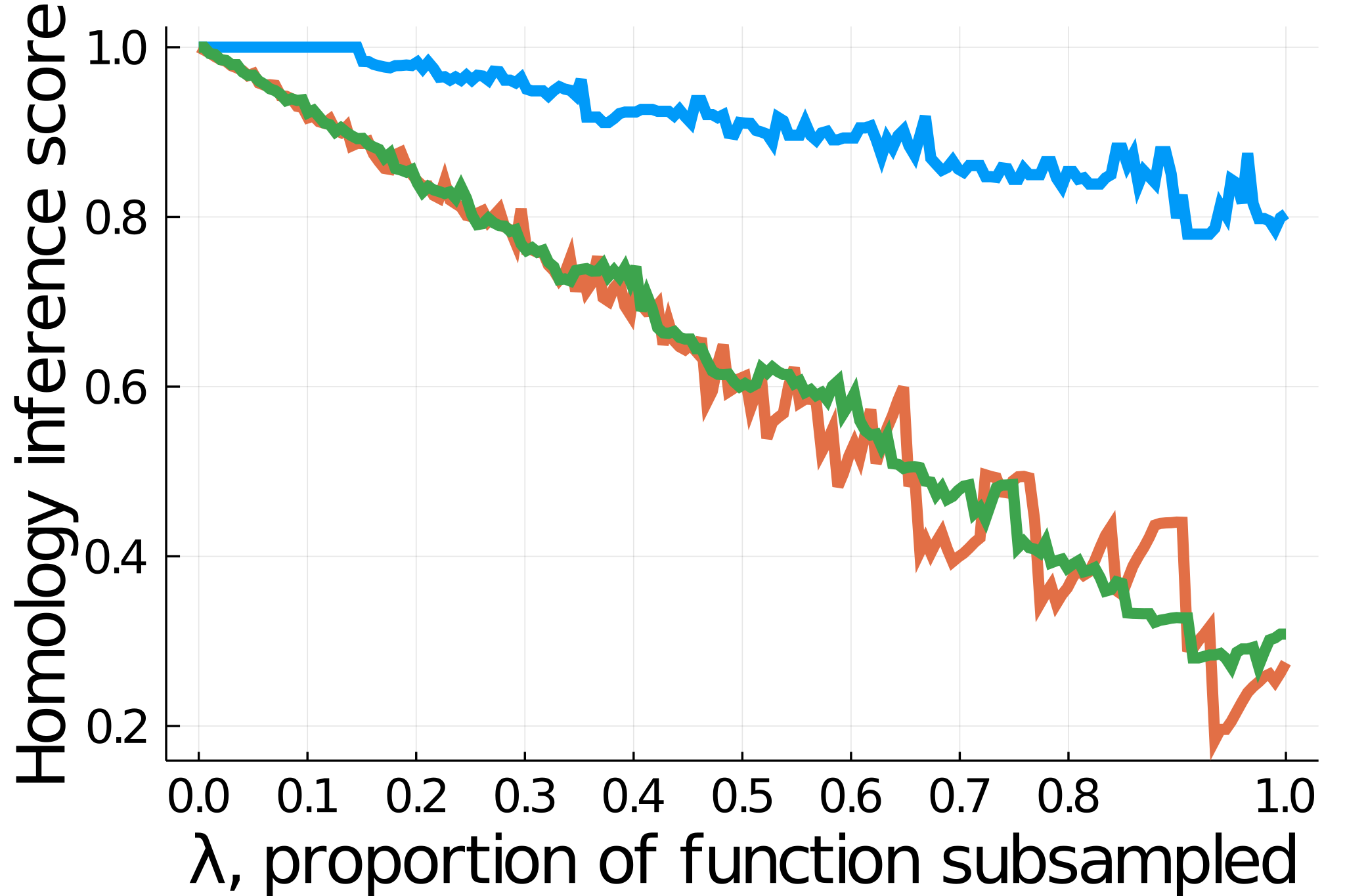
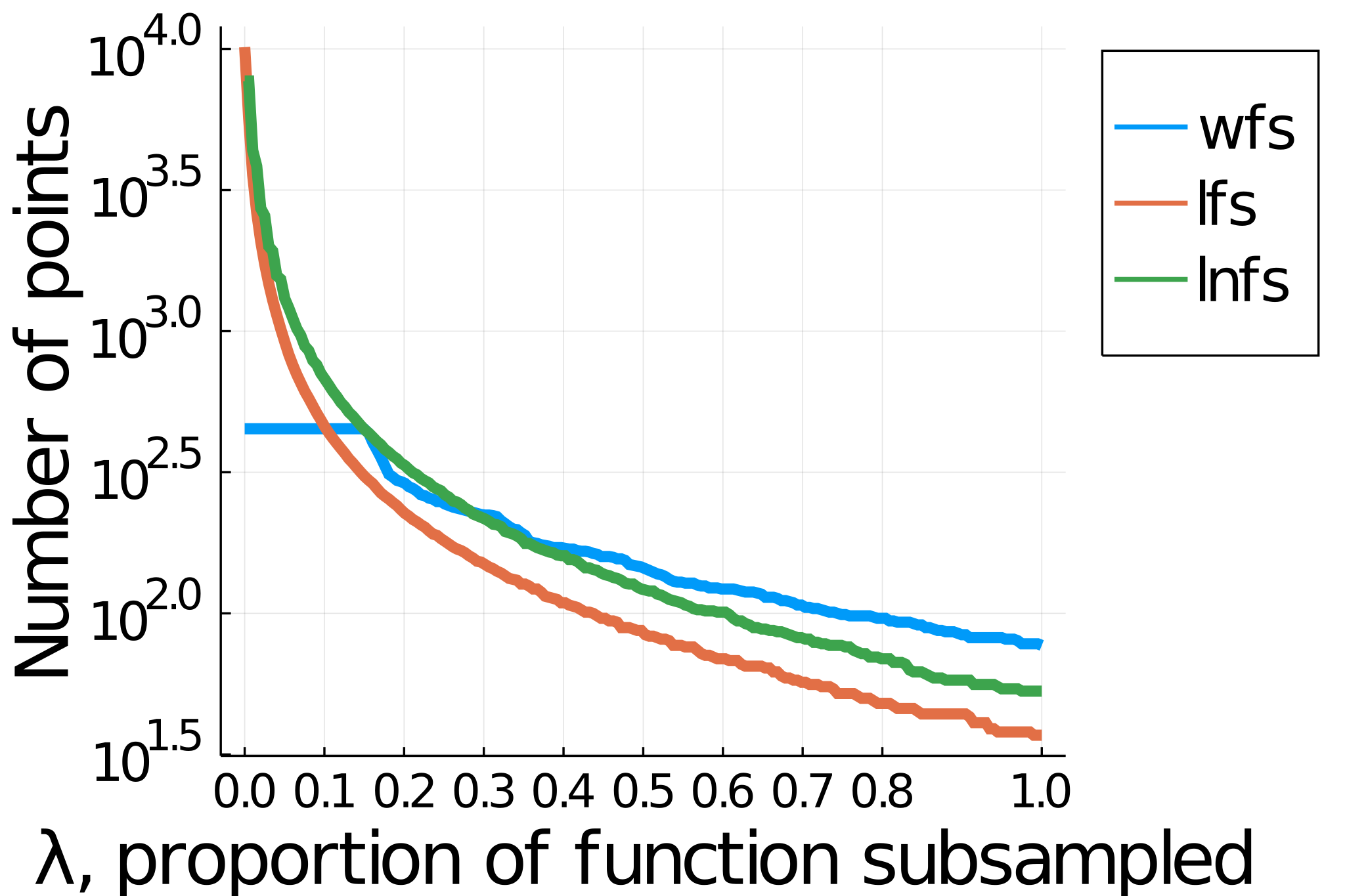
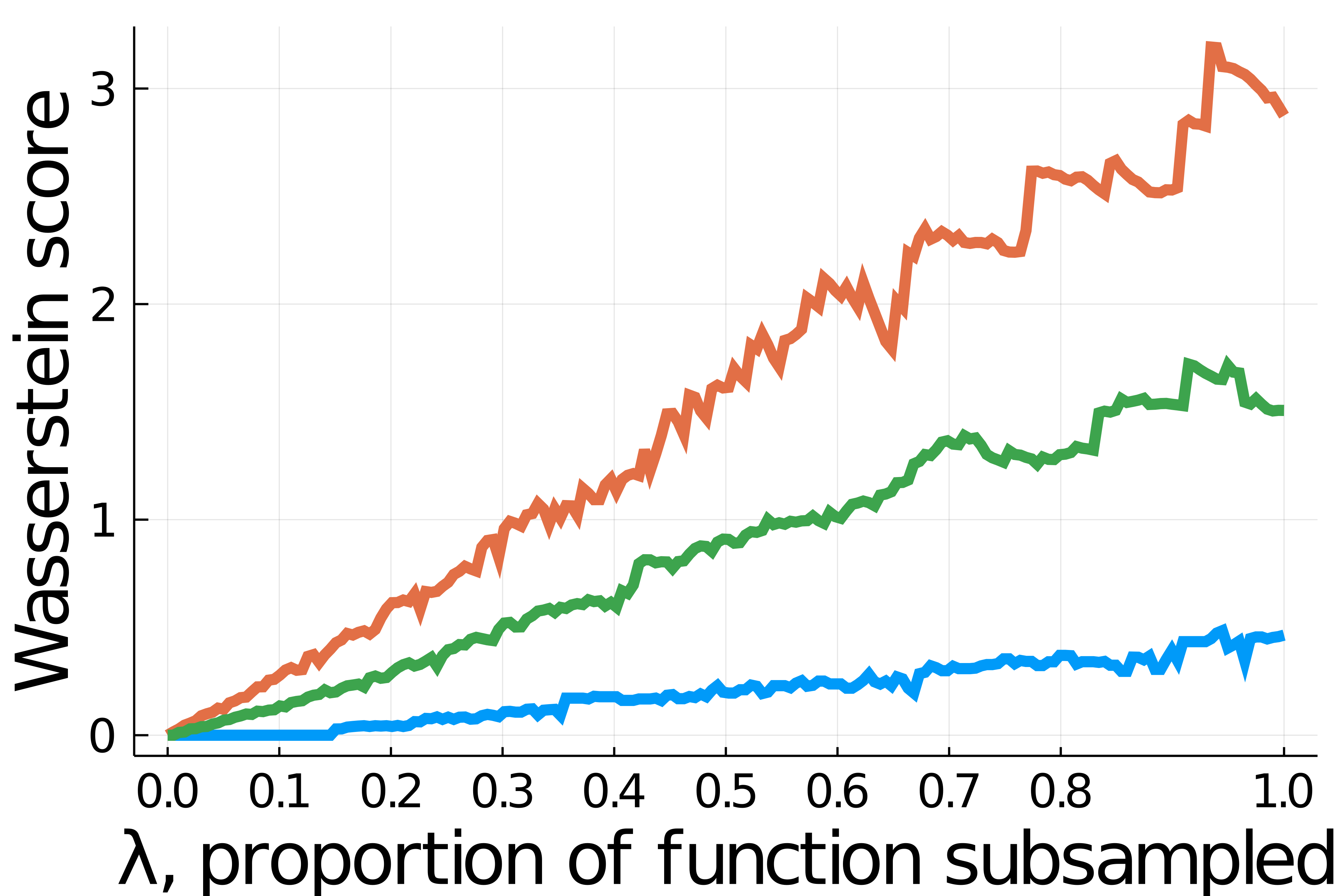
Figure 15: Computational results comparing the behavior of subsampling methods.

Figure 15 records results from experiments that sampled the butterfly curve and computed the scores above. In particular, the $\operatorname{lnfs}$-adaptive subsampling exhibits comparable performance to the $\operatorname{lfs}$-adaptive subsampling method it approximates. Both of these adaptive methods produce subsamples with fewer points than uniform subsampling across a substantial range of subsampling thresholds. We can also see that the persistent homology outputs were less sensitive to the subsampling threshold when conducting uniform subsampling.

7 Conclusion

In this paper, we developed theoretical foundations and numerical algebraic geometry methods for computing geometric feature sizes of algebraic manifolds. We also demonstrated how to combine these methods with persistent homology for both homology inference and for testing geometric algorithms. This study is not intended to be exhaustive, so some further questions both in terms of theory and applications follow.

Real algebraic spaces with singularities. It is natural to ask how the results presented here may generalize to singular spaces. Since isolated singularities can contribute additional irreducible components to $B_{k}(F)$, the impact of singularities must be analyzed.

Counting algebraic bottlenecks. A direct consequence of Theorem 4.15, which will be familiar to readers who have worked with parameter homotopies, is that, for a fixed degree pattern, there exist upper bounds on the number of algebraic (and so geometric) bottlenecks that apply for any generic algebraic manifold with that degree pattern. Computing sharp upper bounds, however, is an open problem of more than intrinsic interest. As an example of the geometric meaning of these bounds, consider a compact algebraic hypersurface $H\subseteq\mathbb{R}^{n}$, not necessarily smooth, e.g., the discriminant locus of a parameterized family. Thus, $\mathbb{R}^{n}\setminus H$ decomposes into a finite number of disconnected $n$-cells and the number of geometric bottlenecks of $H$ is an upper bound on the number of cells. Altogether, having good bounds on this number both for algebraic manifolds and for singular algebraic spaces could be useful for geometric algorithms which look to estimate the number and size of these cells.

Algebraic models and persistent homology. In Section 3, we saw an application where feature sizes are computed to construct samples of an algebraic manifold $X$ for analysis via Vietoris-Rips persistent homology. Instead, consider the persistence module obtained by thickening the space being sampled, i.e., the persistence module $H_{\ell}X^{\bullet}$. Its persistence diagram is constrained by the critical values of $d_{X}$, which we can now compute. That persistence diagram in turn constrains the persistence diagram obtained from Vietoris-Rips persistent homology of a sample [48]. Can these constraints be leveraged to reduce the cost of persistence computations from a sample?

Reducing redundant computations. For any polynomial system $F$, there is an action of the symmetric group on $k$ elements on the bottleneck correspondence $B_{k}(F)$. Namely, a permutation acts on an element $(x_{1},\dots,x_{k},t_{1},\dots,t_{k})$ by permuting both the $x_{i}$ and $t_{i}$. In the generic case when all non-degenerate solutions are isolated, standard homotopy continuation methods whose results we saw in this manuscript compute $k!$ solutions in $B_{k}(F)$ for each algebraic bottleneck. Is there a natural approach, e.g., building on methods utilized in [50, 69, 70], that takes advantage of the symmetry to reduce these redundancies?

Appendix A Appendix

A.1 Proof of Theorem 2.11

Theorem A.1.

Let $A_{n}=\sqrt{\frac{2n}{n+1}}$, let $\hat{X}$ be a $(\delta,\epsilon)$-sample of a real semialgebraic set $X$ in $\mathbb{R}^{n}$, and let $\delta^{\prime}=2\epsilon(A_{n}^{2}-1)+\delta A_{n}$. If $2(\epsilon+\delta^{\prime})<\operatorname{wfs}(X)$ then for $a(\delta,\epsilon)=2\epsilon$ and $b(\delta,\epsilon)=2(2\epsilon A_{n}+\delta)$ the Betti number $\beta_{\ell}(X)$ is the rank of the map obtained from applying $H_{\ell}$ to the inclusion map $R_{\hat{X}}(a(\delta,\epsilon))\subseteq R_{\hat{X}}(b(\delta,\epsilon))$.

Proof.

We have the following chain of simplicial inclusions:

$$C_{\hat{X}}(\epsilon)\subseteq R_{\hat{X}}(2\epsilon)\subseteq C_{\hat{X}}(\epsilon A_{n})\subseteq C_{\hat{X}}(2\epsilon A_{n}+\delta)\subseteq R_{\hat{X}}(2(2\epsilon A_{n}+\delta))$$

$$\subseteq C_{\hat{X}}(A_{n}(2\epsilon A_{n}+\delta))=C(2\epsilon+\delta^{\prime})$$

where inclusions between C̆ech and Vietoris-Rips complexes follow from de Silva and Ghrist’s Theorem [31]. Note that since $\hat{X}$ is a $(\delta,\epsilon)$-sample of $X$, it is also a $(\delta^{\prime},\epsilon)-$sample of $X$ and a $(\delta,\epsilon A_{n})-$sample of $X$ because $\delta^{\prime}\geq\delta$ and $\epsilon A_{n}>\epsilon$. Also note that $2(\epsilon A_{n}+\delta)<2(\epsilon+\delta^{\prime})<\operatorname{wfs}(X)$, the first inequality being easy to verify given $A_{n}>1$ and the second inequality having been assumed. Applying $H_{\ell}$ to the sequence, the linear maps induced by both the internal and external inclusions of C̆ech complexes have rank $\beta_{\ell}(X)$ by Theorem 2.10. By properties of linear maps, these inclusions give an upper and lower bound, respectively, of $\beta_{\ell}(X)$ for $\operatorname{rank}(H_{\ell}R_{\hat{X}})(a(\delta,\epsilon),b(\delta,\epsilon))$. ∎

A.2 Homology inference and subsampling

Recall that for a set $X$ in $\mathbb{R}^{n}$ and $z\in\mathbb{R}^{n}$, $\pi_{X}(z)$ denotes the set of points in $X$ with minimum distance to $z$. Abusing notation, let $\operatorname{lfs}(\pi_{X}(z))$ denote $\inf_{x\in\pi_{X}(z)}\operatorname{lfs}(x)$. This is always a minimum for closed $X$ because $\operatorname{lfs}$ is continuous, in fact 1-Lipschitz continuous.

Definition A.2.

([26]) A finite subset $\hat{X}$ of $\mathbb{R}^{n}$ is an adaptive-$(\alpha,\beta)$ sample of a compact manifold $X$ for $\alpha,\beta>0$ if

• for any $\hat{x}\in\hat{X}$, $d_{X}(\hat{x})<\alpha\beta\operatorname{lfs}(\pi_{X}(\hat{x}))$, and

• for all $x\in X$, there is $\hat{x}\in\hat{X}$ such that $d(x,\pi_{X}(\hat{x}))<\beta\operatorname{lfs}(\pi_{X}(\hat{x}))$.

Definition A.3.

([26]) Suppose $0<\kappa$, $X$ is a compact subspace of $\mathbb{R}^{n}$, and $P$ is a finite subset of $\mathbb{R}^{n}$. For any $z\in\mathbb{R}^{n}$ let $\operatorname{lfs}^{\pi}_{\kappa}(z)=\kappa\operatorname{lfs}(\pi_{X}(z))$. Denote by $K_{P,\operatorname{lfs}^{\pi}}(\kappa)$ the union of balls

$$\cup_{z\in P}\overline{B}_{z}(\operatorname{lfs}^{\pi}_{\kappa}(z))$$

and denote by $C_{P,\operatorname{lfs}^{\pi}}$ the functor $\mathbf{R}\to\mathbf{simp}$ where $C_{P,\operatorname{lfs}^{\pi}}(\kappa)$ is the nerve of $\{\overline{B}_{z}(\operatorname{lfs}^{\pi}_{\kappa}(z))\}_{z\in P}$.

Theorem A.4.

(Chazal and Lieutier [26, Thm. 6.2]) Suppose $\hat{X}$ is an $(\alpha,\beta)-$adaptive sample of a smooth and compact manifold $X$ in $\mathbb{R}^{n}$. There exist functions $g,h:\mathbb{R}^{4}\to\mathbb{R}$ where, if $0<a<b<\frac{1}{3}-\alpha\beta$ and $g(\alpha,\beta,a,b)<h(\alpha,\beta,a,b)$, then $X$ is a deformation retract of $K_{\hat{X},\operatorname{lfs}^{\pi}}(\kappa)$ for $\kappa\in[a,b]$.

The Nerve Theorem applies in the above definition, so that the geometric realization $|C_{P,\operatorname{lfs}^{\pi}}(\kappa)|$ is homotopy equivalent to $K_{P,\operatorname{lfs}^{\pi}}(\kappa)$ for all $P$, $X$, and $\kappa$. The functions $g$ and $h$ in the Theorem are given explicitly by Chazal and Lieutier, and arise from technical geometric considerations.

Our homotopy continuation methods in Section 3 give us oracles for $\operatorname{lfs}$ and the reach, but these require some care to integrate with Theorem A.4. The oracles introduce some estimation error, for instance, and we can only estimate $\operatorname{lfs}(z)$ for a point $z\in\mathbb{R}^{n}$ rather than $\operatorname{lfs}(\pi_{X}(z))$.

To fix notation, let $X$ be a smooth and compact algebraic manifold in $\mathbb{R}^{n}$ that is the real part of an equidimensional and smooth algebraic variety. Let $0<\widehat{\operatorname{lfs}}\leq\operatorname{lfs}_{X}$, let $\|\operatorname{lfs}-\widehat{\operatorname{lfs}}\|_{\infty}\leq E_{\operatorname{lfs}}$, and let $0<R<\operatorname{reach}(X)$. Fix $\delta>0$ and denote $\frac{\delta}{R}$ by $\delta_{R}$. In the following, recall that $\operatorname{lfs}(x)\leq\operatorname{reach}(X)$ for all $x\in X$ and that $\operatorname{lfs}$ is 1-Lipschitz.

Theorem A.5.

Let $0<\lambda,\mu\leq 1$ and let $\hat{X}_{0}$ be a $(\delta_{R}R,\mu R)$-sample of $X$.

1. Take $\beta^{\prime}=\mu+3\delta_{R}+\lambda(1+\delta_{R})$ and $\alpha^{\prime}=\frac{\delta_{R}}{\beta^{\prime}}$. If $\widehat{\operatorname{lfs}}_{\lambda}:\mathbb{R}^{n}\to\mathbb{R}$ is defined by $z\mapsto\lambda\widehat{\operatorname{lfs}}(z)$, then $\textsc{Subsample}(\hat{X}_{0},\widehat{\operatorname{lfs}}_{\lambda})$, denoted $\hat{X}$, is an adaptive-$(\alpha^{\prime},\beta^{\prime})$ sample of $X$.

2. Set $M_{K}=\frac{E_{\operatorname{lfs}}}{R}+\delta_{R}+1$ and $M_{\hat{K}}=\frac{E_{\operatorname{lfs}}}{\hat{R}(1-\delta_{R})}+\frac{1}{1-\delta_{R}}$ where $\hat{R}=\min_{\hat{x}\in\hat{X}}\widehat{\operatorname{lfs}}(\hat{x})$. If there is $a>0$ such that $4(M_{K}M_{\hat{K}})^{2}a<\frac{1}{3}-\delta_{R}$ and $g(\alpha^{\prime},\beta^{\prime},a,4(M_{K}M_{\hat{K}})^{2}a)<h(\alpha^{\prime},\beta^{\prime},a,4(M_{K}M_{\hat{K}})^{2}a)$ where $g$ and $h$ are the functions from Theorem A.4, then the rank of the map

   $$H_{\ell}(R_{\hat{X},\widehat{\operatorname{lfs}}}(M_{k}a)\subseteq R_{\hat{X},\widehat{\operatorname{lfs}}}(2M_{K}^{2}M_{\hat{K}}a))$$

   is the $\ell^{\text{th}}$ Betti number of $X$.

The remainder of the Appendix is dedicated to proving this Theorem.

Proposition A.6.

Let $0\leq\lambda\leq 1$, let $X$ have $0<R<\operatorname{reach}(X)$, let $\hat{X}$ be a $(\delta_{R}R,\mu R)$-sample of $X$ in $\mathbb{R}^{n}$ and let $\widehat{\operatorname{lfs}}_{\lambda}:\mathbb{R}^{n}\to\mathbb{R}$ be defined by $z\mapsto\lambda\widehat{\operatorname{lfs}}(z)$. Take $\beta^{\prime}=\mu+3\delta_{R}+\lambda(1+\delta_{R})$ and $\alpha^{\prime}=\frac{\delta_{R}}{\beta^{\prime}}$. Then $\textsc{Subsample}(\hat{X},\widehat{\operatorname{lfs}}_{\lambda})$ is an adaptive-$(\alpha^{\prime},\beta^{\prime})$ sample of $X$.

Proof.

Denote $\textsc{Subsample}(\hat{X},\widehat{\operatorname{lfs}}_{\lambda})$ by $S$. The first condition of Definition A.2 is trivially satisfied because $S\subseteq\hat{X}$. To see the second condition holds, first suppose $x\in X$. There is $\hat{x}\in\hat{X}$ such that $\|x-\hat{x}\|\leq\mu R$. Therefore $\|x-\pi_{X}(\hat{x})\|\leq(\delta_{R}+\mu)R$. If $\hat{x}\in S$ then the second condition of Definition A.2 is satisfied directly. Otherwise, there is $\hat{x_{0}}\in S$ such that $\|\hat{x_{0}}-\hat{x}\|\leq\lambda\widehat{\operatorname{lfs}}(\hat{x_{0}})\leq\lambda\operatorname{lfs}(\hat{x_{0}})$. We have that

$$\|x-\pi_{X}(\hat{x_{0}})\|\leq\|x-\pi_{X}(\hat{x})\|+\|\pi_{X}(\hat{x})-\pi_{X}(\hat{x_{0}})\|$$

$$\leq\|x-\pi_{X}(\hat{x})\|+\|\pi_{X}(\hat{x_{0}})-\hat{x_{0}}\|+\|\hat{x_{0}}-\hat{x}\|+\|\hat{x}-\pi_{X}(\hat{x})\|$$

$$\leq(\delta_{R}+\mu)R+\delta_{R}R+\lambda\operatorname{lfs}(\hat{x_{0}})+\delta_{R}R$$

$$=R(\mu+3\delta_{R})+\lambda(\operatorname{lfs}(\hat{x_{0}})-\operatorname{lfs}(\pi_{X}(\hat{x_{0}})))+\lambda\operatorname{lfs}(\pi_{X}(\hat{x_{0}}))$$

$$\leq\operatorname{lfs}(\pi_{X}(\hat{x_{0}}))(\mu+3\delta_{R}+\lambda)+\lambda\|\hat{x_{0}}-\pi_{X}(\hat{x_{0}})\|$$

$$\leq\operatorname{lfs}(\pi_{X}(\hat{x_{0}}))(\mu+3\delta_{R}+\lambda(1+\delta_{R}))\text{.}$$

∎

Definition A.7.

Let $X\subseteq\mathbb{R}^{n}$ be compact and the real part of a smooth and equidimensional algebraic variety, let $P$ be a finite subset of $\mathbb{R}^{n}$, and let $\widehat{\operatorname{lfs}}:\mathbb{R}^{n}\to\mathbb{R}$ be the local feature size oracle for $X$ described in Section 3. For $\kappa$ with $0<\kappa$ and any $z\in\mathbb{R}$, let $\widehat{\operatorname{lfs}}_{\kappa}=\kappa\widehat{\operatorname{lfs}}(z)$. Denote by $K_{P,\widehat{\operatorname{lfs}}}(\kappa)$ the union of balls

$$\cup_{z\in P}\overline{B}_{z}(\widehat{\operatorname{lfs}}_{\kappa}(z))$$

and denote by $C_{P,\widehat{\operatorname{lfs}}}$ the functor $\mathbf{R}\to\mathbf{simp}$ where $C_{P,\widehat{\operatorname{lfs}}}(\kappa)$ is the nerve of $\{\overline{B}_{z}(\widehat{\operatorname{lfs}}_{\kappa}(z))\}_{z\in P}$.

Remark A.8.

Let $0\leq\alpha^{\prime},\beta^{\prime}<1$ and let $\hat{X}$ be an adaptive-$(\alpha^{\prime},\beta^{\prime})$ sample of $X$ in $\mathbb{R}^{n}$. Since $\operatorname{lfs}$ is 1-Lipschitz we have for any $\hat{x}\in\hat{X}$ that $\operatorname{lfs}(\hat{x})-\operatorname{lfs}(\pi_{X}(\hat{x}))\leq\|\hat{x}-\pi_{X}(\hat{x})\|\leq\alpha^{\prime}\beta^{\prime}\operatorname{lfs}(\pi_{X}(\hat{x}))$. This rearranges to $\operatorname{lfs}(\pi_{X}(\hat{x}))\leq\frac{1}{1-\alpha^{\prime}\beta^{\prime}}\operatorname{lfs}(\hat{x})$.

Proposition A.9.

Let $\hat{X}$ be an adaptive-$(\alpha^{\prime},\beta^{\prime})$ sample of $X$ with $0\leq\alpha^{\prime}\beta^{\prime}<1$ and let $\hat{R}=\min_{\hat{x}\in X}\hat{\operatorname{lfs}}(\hat{x})$. Set $M_{K}=\frac{E_{\operatorname{lfs}}}{R}+\alpha^{\prime}\beta^{\prime}+1$ and $M_{\hat{K}}=\frac{E_{\operatorname{lfs}}}{\hat{R}(1-\alpha^{\prime}\beta^{\prime})}+\frac{1}{1-\alpha^{\prime}\beta^{\prime}}$. Then for any $\kappa>0$, $K_{\hat{X},\operatorname{lfs}^{\pi}}(\kappa)\subseteq K_{\hat{X},\widehat{\operatorname{lfs}}}(M_{\hat{K}}\kappa)$ and $\hat{K}_{\hat{X},\widehat{\operatorname{lfs}}}(\kappa)\subseteq K_{\hat{X},\operatorname{lfs}^{\pi}}(M_{K}\kappa).$

Proof.

For the first inclusion, suppose $y\in\mathbb{R}^{n}$ has $\|y-\hat{x}\|\leq\kappa\operatorname{lfs}(\pi_{X}(\hat{x}))$ for some $\hat{x}\in\hat{X}$. Hence,

$$\|y-\hat{x}\|\leq\frac{\kappa}{1-\alpha^{\prime}\beta^{\prime}}\operatorname{lfs}(\hat{x})=\frac{\kappa}{1-\alpha^{\prime}\beta^{\prime}}(\operatorname{lfs}(\hat{x})-\widehat{\operatorname{lfs}}(\hat{x})+\widehat{\operatorname{lfs}}(\hat{x}))$$

$$\leq\frac{\kappa}{1-\alpha^{\prime}\beta^{\prime}}(E_{\operatorname{lfs}}+\widehat{\operatorname{lfs}}(\hat{x}))\leq\frac{\kappa\widehat{\operatorname{lfs}}(\hat{x})}{1-\alpha^{\prime}\beta^{\prime}}\left(\frac{E_{\operatorname{lfs}}}{\hat{R}}+1\right)\text{.}$$

For the second inclusion, suppose $y\in\mathbb{R}^{n}$ has $\|y-\hat{x}\|\leq\kappa\widehat{\operatorname{lfs}}(\hat{x})$ for some $\hat{x}\in\hat{X}$. Then

$$\|y-\hat{x}\|\leq\kappa(\widehat{\operatorname{lfs}}(\hat{x})-\operatorname{lfs}(\hat{x})+\operatorname{lfs}(\hat{x}))\leq\kappa(E_{\operatorname{lfs}}+\operatorname{lfs}(\hat{x})-\operatorname{lfs}(\pi_{X}(\hat{x}))+\operatorname{lfs}(\pi_{X}(\hat{x})))$$

$$\leq\kappa(E_{\operatorname{lfs}}+\|\hat{x}-\pi_{X}(\hat{x})\|+\operatorname{lfs}(\pi_{X}(\hat{x})))\leq\kappa(E_{\operatorname{lfs}}+\alpha^{\prime}\beta^{\prime}\operatorname{lfs}(\pi_{X}(\hat{x}))+\operatorname{lfs}(\pi_{X}(\hat{x})))$$

$$\leq\kappa\operatorname{lfs}(\pi_{X}(\hat{x}))\left(\frac{E_{\operatorname{lfs}}}{R}+\alpha^{\prime}\beta^{\prime}+1\right).$$

∎

Corollary A.10.

With notation and assumptions as in Proposition A.9, let

$$M_{K}=\left(\frac{E_{\operatorname{lfs}}}{\hat{R}}+1\right)\frac{1}{1-\alpha^{\prime}\beta^{\prime}}\hbox{~{}~{}and~{}~{}}M_{\hat{K}}=\frac{E_{\operatorname{lfs}}}{R}+\alpha^{\prime}\beta^{\prime}+1.$$

Suppose that $0<a<(M_{K}M_{\hat{K}})^{2}a<\frac{1}{3}-\alpha^{\prime}\beta^{\prime}$ and

$$g(\alpha^{\prime},\beta^{\prime},a,(M_{k}M_{\hat{K}})^{2}a)\leq h(\alpha^{\prime},\beta^{\prime},a,(M_{k}M_{\hat{K}})^{2}a).$$

Then, the Betti number $\beta_{\ell}(X)$ is the rank of the map obtain from applying $H_{\ell}$ to the inclusion $C_{\hat{X},\widehat{\operatorname{lfs}}}(M_{K}a)\subseteq C_{\hat{X},\widehat{\operatorname{lfs}}}(M_{K}^{2}M_{\hat{K}}a)$.

Proof.

The former Proposition gives us the chain of inclusions

$${K}_{\hat{X},\operatorname{lfs}^{\pi}}(a)\subseteq K_{\hat{X},\widehat{\operatorname{lfs}}}(M_{\hat{K}}a)\subseteq{K}_{\hat{X},\operatorname{lfs}^{\pi}}(M_{\hat{K}}M_{K}a)\subseteq K_{\hat{X},\widehat{\operatorname{lfs}}}(M_{\hat{K}}^{2}M_{K}a)\subseteq{K}_{\hat{X},\operatorname{lfs}^{\pi}}((M_{\hat{K}}M_{K})^{2}a)\text{.}$$

By applying Theorem A.4 we have that all the spaces $K_{\hat{X},\operatorname{lfs}^{\pi}}$ deformation retract to $X$. Applying the nerve lemma we can replace $K$ with $C$. ∎

Proposition A.11.

With notation and assumptions as in Corollary A.10 except with $4(M_{K}M_{\hat{K}})^{2}$ replacing $(M_{K}M_{\hat{K}})^{2}$, the Betti number $\beta_{\ell}(X)$ is the rank of the map obtained from applying $H_{\ell}$ to the inclusion $R_{\hat{X},\widehat{\operatorname{lfs}}}(M_{K}a)\subseteq R_{\hat{X},\widehat{\operatorname{lfs}}}(2M_{K}^{2}M_{\hat{K}}a)$.

Proof.

For any $\kappa$ we have the following inclusions. Use them to produce a 6-term inclusion chain similarly to the proof of Theorem 2.11:

$$C_{\hat{X},\widehat{\operatorname{lfs}}}(\kappa)\subseteq R_{\hat{X},\widehat{\operatorname{lfs}}}(\kappa)\subseteq C_{\hat{X},\widehat{\operatorname{lfs}}}(2\kappa)\text{.}$$

∎

References

- [1] E. Aamari, J. Kim, F. Chazal, B. Michel, A. Rinaldo, and L. Wasserman. Estimating the reach of a manifold. Electron. J. Stat., 13(1):1359–1399, 2019.
- [2] J. Alexander and A. Hirschowitz. Polynomial interpolation in several variables. J. Algebraic Geom., 4(2):201–222, 1995.
- [3] N. Amenta and M. Bern. Surface reconstruction by voronoi filtering. Discrete & Computational Geometry, 22(4):481–504, 1999.
- [4] D. Attali, A. Lieutier, and D. Salinas. Vietoris-Rips complexes also provide topologically correct reconstructions of sampled shapes. Comput. Geom., 46(4):448–465, 2013.
- [5] S. Basu. Computing the first few Betti numbers of semi-algebraic sets in single exponential time. Journal of Symbolic Computation, 41(10):1125–1154, 2006.
- [6] S. Basu and S. Percival. Efficient computation of a semi-algebraic basis of the first homology group of a semi-algebraic set. arXiv:2107.08947, 2021.
- [7] D. J. Bates, D. Eklund, J. D. Hauenstein, and C. Peterson. Excess intersections and numerical irreducible decompositions. In 2021 23rd International Symposium on Symbolic and Numeric Algorithms for Scientific Computing (SYNASC), pages 52–60, 2021.
- [8] D. J. Bates, J. D. Hauenstein, T. M. McCoy, C. Peterson, and A. J. Sommese. Recovering exact results from inexact numerical data in algebraic geometry. Experimental Mathematics, 22(1):38–50, 2013.
- [9] D. J. Bates, J. D. Hauenstein, C. Peterson, and A. J. Sommese. Numerical decomposition of the rank-deficiency set of a matrix of multivariate polynomials. In Approximate Commutative Algebra, Texts Monogr. Symbol. Comput., pages 55–77. Springer, Vienna, 2009.
- [10] D. J. Bates, J. D. Hauenstein, A. J. Sommese, and C. W. Wampler. Numerically solving polynomial systems with Bertini, volume 25. SIAM, 2013.
- [11] D. J. Bates, J. D. Hauenstein, A. J. Sommese, and C. W. Wampler. Bertini: Software for numerical algebraic geometry. Available at bertini.nd.edu with permanent doi: dx.doi.org/10.7274/R0H41PB5, 2014.
- [12] U. Bauer. Ripser. https://github.com/Ripser/ripser, 2016.
- [13] U. Bauer. Ripser: efficient computation of Vietoris-Rips persistence barcodes. J. Appl. Comput. Topol., 5(3):391–423, 2021.
- [14] O. Bobrowski and R. J. Adler. Distance functions, critical points, and the topology of random Čech complexes. Homology Homotopy Appl., 16(2):311–344, 2014.
- [15] M. Brandt and M. Weinstein. Voronoi cells in metric algebraic geometry of plane curves. arXiv preprint arXiv:1906.11337, 2019.
- [16] P. Breiding and S. Timme. The reach of a plane curve. https://www.JuliaHomotopyContinuation.org/examples/reach-curve/. Accessed: January 21, 2022.
- [17] P. Breiding and S. Timme. Homotopycontinuation.jl: A package for homotopy continuation in julia. In J. H. Davenport, M. Kauers, G. Labahn, and J. Urban, editors, Mathematical Software – ICMS 2018, pages 458–465, Cham, 2018. Springer International Publishing.
- [18] P. Bürgisser, F. Cucker, and P. Lairez. Computing the homology of basic semialgebraic sets in weak exponential time. J. ACM, 66(1):Art. 5, 30, 2019. [Publication date initially given as 2018].
- [19] C. Carathéodory. Über den variabilitätsbereich der fourier’schen konstanten von positiven harmonischen funktionen. Rendiconti Del Circolo Matematico di Palermo (1884-1940), 32(1):193–217, 1911.
- [20] G. Carlsson. Topology and data. Bulletin of the American Mathematical Society, 46(2):255–308, 2009.
- [21] J.-D. Cassini. De l’Origine et du progrès de l’astronomie et de son usage dans la géographie et dans la navigation. L’Imprimerie Royale, 1693. Accessed online 2021-05-27, https://gallica.bnf.fr/ark:/12148/bpt6k1510911j/f13.item, page 36.
- [22] N. J. Cavanna. Methods in Homology Inference. PhD thesis, University of Connecticut, 2019.
- [23] N. J. Cavanna and D. R. Sheehy. Adaptive metrics for adaptive samples. Algorithms, 13(8):200, 2020.
- [24] F. Chazal, D. Cohen-Steiner, M. Glisse, L. J. Guibas, and S. Y. Oudot. Proximity of persistence modules and their diagrams. In Proceedings of the twenty-fifth annual symposium on Computational geometry, pages 237–246. ACM, 2009.
- [25] F. Chazal and A. Lieutier. Weak feature size and persistent homology: computing homology of solids in from noisy data samples. In Proceedings of the twenty-first annual symposium on Computational geometry, pages 255–262. ACM, 2005.
- [26] F. Chazal and A. Lieutier. Smooth manifold reconstruction from noisy and non-uniform approximation with guarantees. Comput. Geom., 40(2):156–170, 2008.
- [27] F. Chazal and B. Michel. An introduction to topological data analysis: Fundamental and practical aspects for data scientists. Frontiers in Artificial Intelligence, page 108, 2021.
- [28] A. Clebsch. Ueber die Anwendung der quadratischen Substitution auf die Gleichungen 5 ten Grades und die geometrische Theorie des ebenen Fünfseits. Math. Ann., 4(2):284–345, 1871.
- [29] D. Cohen-Steiner, H. Edelsbrunner, and J. Harer. Stability of persistence diagrams. Discrete Comput. Geom., 37(1):103–120, 2007.
- [30] M. Čufar. Ripserer.jl: flexible and efficient persistent homology computation in Julia. Journal of Open Source Software, 5(54):2614, 2020.
- [31] V. De Silva and R. Ghrist. Coverage in sensor networks via persistent homology. Algebraic & Geometric Topology, 7(1):339–358, 2007.
- [32] T. K. Dey, Z. Dong, and Y. Wang. Parameter-free topology inference and sparsification for data on manifolds. In Proceedings of the Twenty-Eighth Annual ACM-SIAM Symposium on Discrete Algorithms, pages 2733–2747. SIAM, Philadelphia, PA, 2017.
- [33] T. K. Dey, X. Ge, Q. Que, I. Safa, L. Wang, and Y. Wang. Feature-preserving reconstruction of singular surfaces. In Computer Graphics Forum, volume 31, pages 1787–1796. Wiley Online Library, 2012.
- [34] S. Di Rocco, D. Eklund, and O. Gäfvert. Sampling and homology via bottlenecks. Mathematics of Computations, to appear, 2022.
- [35] S. Di Rocco, D. Eklund, and M. Weinstein. The bottleneck degree of algebraic varieties. SIAM J. Appl. Algebra Geom., 4(1):227–253, 2020.
- [36] E. Dufresne, P. Edwards, H. Harrington, and J. Hauenstein. Sampling real algebraic varieties for topological data analysis. In 2019 18th IEEE International Conference On Machine Learning And Applications (ICMLA), pages 1531–1536. IEEE, 2019.
- [37] H. Edelsbrunner and J. Harer. Computational topology: an introduction. American Mathematical Soc., 2010.
- [38] D. Eklund. The numerical algebraic geometry of bottlenecks. Advances in Applied Mathematics, 142:102416, 2023.
- [39] H. Federer. Curvature measures. Trans. Amer. Math. Soc., 93:418–491, 1959.
- [40] M. Fiedler. Matrices and graphs in geometry, volume 139 of Encyclopedia of Mathematics and its Applications. Cambridge University Press, Cambridge, 2011.
- [41] J. H. G. Fu. Tubular neighborhoods in Euclidean spaces. Duke Math. J., 52(4):1025–1046, 1985.
- [42] V. Gershkovich and H. Rubinstein. Morse theory for Min-type functions. Asian J. Math., 1(4):696–715, 1997.
- [43] R. Ghrist. Barcodes: the persistent topology of data. Bulletin of the American Mathematical Society, 45(1):61–75, 2008.
- [44] B. Giunti. Tda-applications: A database for application of tda outside of maths. https://www.zotero.org/groups/2425412/tda-applications. Accessed: August 2022.
- [45] K. Grove. Critical point theory for distance functions. In Differential geometry: Riemannian geometry (Los Angeles, CA, 1990), volume 54 of Proc. Sympos. Pure Math., pages 357–385. Amer. Math. Soc., Providence, RI, 1993.
- [46] K. Grove and K. Shiohama. A generalized sphere theorem. Ann. of Math. (2), 106(2):201–211, 1977.
- [47] O. Hanner. Some theorems on absolute neighborhood retracts. Ark. Mat., 1:389–408, 1951.
- [48] S. Harker, M. Kramár, R. Levanger, and K. Mischaikow. A comparison framework for interleaved persistence modules. Journal of applied and computational topology, 3(1):85–118, 2019.
- [49] J. D. Hauenstein. Numerically computing real points on algebraic sets. Acta Applicandae Mathematicae, 125:105–119, 2013.
- [50] J. D. Hauenstein, L. Oeding, G. Ottaviani, and A. J. Sommese. Homotopy techniques for tensor decomposition and perfect identifiability. Journal für die reine und angewandte Mathematik (Crelles Journal), 2019(753):1–22, 2019.
- [51] J. D. Hauenstein, A. J. Sommese, and C. W. Wampler. Regeneration homotopies for solving systems of polynomials. Math. Comp., 80(273):345–377, 2011.
- [52] J. D. Hauenstein, A. J. Sommese, and C. W. Wampler. Regenerative cascade homotopies for solving polynomial systems. Applied Mathematics and Computation, 218(4):1240–1246, 2011.
- [53] F. Hensel, M. Moor, and B. Rieck. A survey of topological machine learning methods. Frontiers in Artificial Intelligence, 4:681108, 2021.
- [54] E. Horobeţ. The critical curvature degree of an algebraic variety. arXiv preprint arXiv:2104.01124, 2021.
- [55] E. Horobeţ and M. Weinstein. Offset hypersurfaces and persistent homology of algebraic varieties. Computer Aided Geometric Design, 74:101767, 2019.
- [56] J. Kim, J. Shin, F. Chazal, A. Rinaldo, and L. Wasserman. Homotopy reconstruction via the Cech complex and the Vietoris-Rips complex. In 36th International Symposium on Computational Geometry, volume 164 of LIPIcs. Leibniz Int. Proc. Inform., pages Art. No. 54, 19. Schloss Dagstuhl. Leibniz-Zent. Inform., Wadern, 2020.
- [57] S. Lojasiewicz. Triangulation of semi-analytic sets. Ann. Scuola Norm. Sup. Pisa Cl. Sci. (3), 18:449–474, 1964.
- [58] J. Milnor. Morse theory. Annals of Mathematics Studies, No. 51. Princeton University Press, Princeton, N.J., 1963. Based on lecture notes by M. Spivak and R. Wells.
- [59] A. P. Morgan and A. J. Sommese. Coefficient-parameter polynomial continuation. Appl. Math. Comput., 29(2, part II):123–160, 1989.
- [60] A. P. Morse. The behavior of a function on its critical set. Ann. of Math. (2), 40(1):62–70, 1939.
- [61] M. Morse. The calculus of variations in the large, volume 18. American Mathematical Soc., 1934.
- [62] P. Niyogi, S. Smale, and S. Weinberger. Finding the Homology of Submanifolds with High Confidence from Random Samples. Discrete & Computational Geometry, 39(1-3):419–441, 2008.
- [63] N. Otter, M. A. Porter, U. Tillmann, P. Grindrod, and H. A. Harrington. A roadmap for the computation of persistent homology. EPJ Data Science, 6(1):17, 2017.
- [64] S. Y. Oudot. Persistence theory: from quiver representations to data analysis, volume 209. American Mathematical Society, 2015.
- [65] A. Sard. The measure of the critical values of differentiable maps. Bull. Amer. Math. Soc., 48:883–890, 1942.
- [66] A. J. Sommese and J. Verschelde. Numerical homotopies to compute generic points on positive dimensional algebraic sets. Journal of Complexity, 16(3):572–602, 2000.
- [67] A. J. Sommese and C. W. Wampler, II. The Numerical Solution of Systems of Polynomials Arising in Engineering and Science. World Scientific Publishing Co. Pte. Ltd., Hackensack, NJ, 2005.
- [68] E. VanderZee, A. N. Hirani, D. Guoy, V. Zharnitsky, and E. A. Ramos. Geometric and combinatorial properties of well-centered triangulations in three and higher dimensions. Comput. Geom., 46(6):700–724, 2013.
- [69] J. Verschelde and R. Cools. Symmetric homotopy construction. Journal of Computational and Applied Mathematics, 50(1):575–592, 1994.
- [70] C. W. Wampler, A. P. Morgan, and A. J. Sommese. Complete Solution of the Nine-Point Path Synthesis Problem for Four-Bar Linkages. Journal of Mechanical Design, 114(1):153–159, 1992.
- [71] L. Wasserman. Topological data analysis. Annual Review of Statistics and Its Application, 5(1):501–532, 2018.
- [72] R. C. Yates. A Handbook on Curves and Their Properties. J. W. Edwards, Ann Arbor, Michigan, 1947.