Joint Linear and Nonlinear Computation across Functions for Efficient Privacy-Preserving Neural Network Inference

Abstract

While it is encouraging to witness the recent development in privacy-preserving Machine Learning as a Service (MLaaS), there still exists a significant performance gap for its deployment in real-world applications. We observe the state-of-the-art frameworks follow a compute-and-share principle for every function output where the summing in linear functions, which is the last of two steps for function output, involves all rotations (which is the most expensive HE operation), and the multiplexing in nonlinear functions, which is also the last of two steps for function output, introduces noticeable communication rounds. Therefore, we challenge the conventional compute-and-share logic and introduce the first joint linear and nonlinear computation across functions that features by 1) the PHE triplet for computing the nonlinear function, with which the multiplexing is eliminated; 2) the matrix encoding to calculate the linear function, with which all rotations for summing is removed; and 3) the network adaptation to reassemble the model structure, with which the joint computation module is utilized as much as possible. The boosted efficiency is verified by the numerical complexity, and the experiments demonstrate up to 13$\times$ speedup for various functions used in the state-of-the-art models and up to 5$\times$ speedup over mainstream neural networks.

1 Introduction

Deep Learning (DL) has dramatically evolved in the recent decade [1, 2, 3, 4] and been successfully deployed in many applications such as image classification [5], voice recognition [6] and financial evaluation [7]. Due to the need for massive training data and adequate computation resources [8], it is often impractical for an end user (the client $\mathcal{C}$) to train her DL model. To this end, the Machine Learning as a Service (MLaaS) emerges as a feasible alternative where a server $\mathcal{S}$ in the cloud owns a neural network that is well trained on plenty of data, and the client uploads her input to the server to obtain the prediction result.

However, noticeable privacy concerns raise in MLaaS since the client must send her private data, which could be sensitive, to the server. In many cases, the client prefers to obtain the prediction without letting other parties, including the cloud server, know her data. In fact, regulations have been enforced to forbid the disclosure of private data, e.g., the Health Insurance Portability and Accountability Act (HIPAA) [9] for medical data and the General Data Protection Regulation (GDPR) [10] for business data. Meanwhile, the cloud server intends to hide the proprietary parameters of its well-trained neural network, and only return the model output in response to the client’s prediction request.

Privacy-preserving MLaaS takes both legal and ethical concerns for the client’s private data and the server’s model parameters into account, which aims to ensure that 1) the server learns nothing about the client’s private data and 2) the client learns nothing about the server’s model parameters beyond what can be returned from the network output, e.g., the predicted class. The key challenge in privacy-preserving MLaaS is how to efficiently embed cryptographic primitives into function computation of neural networks, which otherwise may lead to prohibitively high computation complexity and/or degraded prediction accuracy due to large-size circuits and/or function approximations.

To achieve usable privacy-preserving MLaaS, a series of recent works have made inspiring progress towards the system efficiency [11, 12, 13, 14, 15, 16, 17, 18, 19, 20, 21, 22, 23, 24, 25]. Specifically, the inference speed has gained several orders of magnitude from CryptoNets [11] to the recent frameworks. At a high level, these privacy-preserving frameworks carefully consider and adopt several cryptographic primitives (e.g., the Homomorphic Encryption (HE) [26, 27, 28] and Multi-Party Computation (MPC) techniques [29] (such as Oblivious Transfer (OT) [30], Secret Sharing (SS) [31] and Garbled Circuits (GC) [32, 33])) to compute the linear (e.g., dot product and convolution) and nonlinear (e.g., ReLU) functions, which are repeatedly stacked and act as the building blocks in a neural network. Among them, the mixed-protocol approaches that utilizes HE to compute linear functions while adapting MPC for nonlinear functions show more efficiency advantages for the privacy-preserving MLaaS with two-party computation [12, 13, 17]. For example, CrypTFlow2 [17] has shown significant speedup compared with other state-of-the-art schemes such as GAZELLE [13] and DELPHI [16].

While it is encouraging to witness the recent development in privacy-preserving MLaaS, there still exists a significant performance gap for its deployment in real-world applications. For example, our benchmark has shown that CrypTFlow2 takes 115 seconds and 147 seconds to run the well-known DL networks VGG-19 [3] and ResNet-34 [4] on the Intel(R) Xeon(R) E5-2666 v3 $@$ 2.90GHz CPU (see the detailed experimental settings and results in Sec. 4). It is worth pointing out that the constraints of response time in many practical ML-driven applications (such as speech recognition and wearable health monitoring) are within a few seconds or up to one minute [34, 35]. This performance gap motivates us to further improve the efficiency of privacy-preserving MLaaS especially for the mixed-protocol approaches.

We begin with analyzing the computation logic in these state-of-the-art privacy-preserving frameworks. Concretely, the basic logic in all designs is to firstly calculate the output of a function, based on specific cryptographic primitives. That securely computed output is in an “encrypted” form and is then shared between $\mathcal{C}$ and $\mathcal{S}$. The respective share at $\mathcal{C}$ and $\mathcal{S}$ acts as the input of next function. As a neural network consists of stacked linear and nonlinear functions, this compute-and-share logic for each function output is sequentially repeated until the last one. For example, the initial input of CrypTFlow2 is $\mathcal{C}$’s private data, which is encrypted and sent to $\mathcal{S}$. $\mathcal{S}$ conducts HE-based computation for the linear function where the HE addition, multiplication, and rotation (which are three basic operators over encrypted data) are performed between $\mathcal{C}$-encrypted data and $\mathcal{S}$’s model parameters. It produces an encrypted function output which is then shared (in plaintext) between $\mathcal{C}$ and $\mathcal{S}$, and those shares serve as the input of the following OT-based computation for subsequent nonlinear function, whose corresponding output shares act as the input for the next function. This computation mode is repeated in function wise until $\mathcal{C}$ gets the network output.

While this compute-and-share mode for each function output is seemly logical and all of the aforementioned works follow this principle, we observe the fact that the summing in linear functions, which is the last of two steps (where the first step is multiplication) to get the function output, involves all rotations (which is the most expensive HE operation), and the multiplexing in nonlinear functions, which is also the last of two steps (where the first step is comparison) to get the function output, introduces noticeable communication rounds (e.g., about one third in OT-based communication rounds [17]). Therefore we ask the following natural question:

Is it possible to efficiently circumvent the compute-and-share logic for the function output such that we can evade expensive r- otations and noticeable communication rounds at the last step of function computation to achieve more efficient privacy-preservi-  ng MLaaS?

Our Contributions. In this paper, we give an affirmative answer to this question. To this end, we challenge and break the conventional compute-and-share logic for function output, and propose the new share-in-the-middle logic towards function computation for efficient privacy-preserving MLaaS. In particular, we come up with the first joint linear and nonlinear computation across functions where the expensive rotations and noticeable communication rounds at the last step of function computation are efficiently removed, via a careful utilization of the intermediates during the function computation. The underlying bases of our joint computation across functions feature with the following three novel designs:

1. the PHE triplet for computing the intermediates of nonlinear function, with which the communication cost for multiplexing is totally eliminated. Meanwhile, it is not only offline-oriented (i.e., its generation is completely independent of $\mathcal{C}$’s private input) but also non-interactive (i.e., its generation is fully asynchronous between $\mathcal{C}$ and $\mathcal{S}$), which is much more flexible compared with other offline-but-synchronous generation [12, 16].

2. the matrix encoding to calculate the intermediates of linear function, with which all rotations for summing is totally removed. For instance, 2048 rotations are needed to calculate one of the convolutions in  ResNet [4] while we save this cost via the proposed matrix encoding. Furthermore, the PHE triplet is integrated with the matrix encoding to form our joint computation block (to be discussed in Sec. 3.2), which shows better efficiency from both numerical and experimental analysis.

3. the network adaptation to reassemble the DL architecture (e.g., adjust the function orders and decompose the function computation to make it integrated with both previous and subsequent functions) such that the recombined functions are more suitable for applying the proposed PHE triplet and matrix encoding, and thus can take more advantages of our proposed joint computation block, which finally contributes to the overall efficiency improvement.

The boosted efficiency of our protocol is demonstrated by both the numerical complexity analysis and the experimental results. For example, we achieve up to 13$\times$ speedup for various functions used in the state-of-the-art DL models and up to $5\times$ speedup over mainstream neural networks, compared with the state-of-the-art privacy-preserving frameworks. Furthermore, we lay our work as an initial attempt for the share-in-the-middle computation, which could inspire more works in this new lane for efficient privacy-preserving MLaaS.

On the other hand, we also notice two most recent works that demonstrate comparable efficiency as ours. The first one is COINN [36] which features with the well-designed model customization and ciphertext execution, and our computation can be built on top of COINN’s quantized models to gain more speedup. The second one is Cheetah [37] which utilizes the accumulative property of polynomial multiplication and the ciphertex extraction to eliminate rotations and relies on VOLE-style OT to boost the nonlinear computation. While we can also benefit from the optimized OT to compute nonlinear functions, we differentiate our work from Cheetah’s rotation elimination by exploiting the accumulative nature in matrix-vector multiplication where the output can be viewed as the linear combination of all columns in the weight matrix. Furthermore, both COINN and Cheetah are under the compute-and-share logic while we set our work as the first one for share-in-the-middle computation.

The rest of the paper is organized as follows. In Sec. 2, we introduce the system setup and the primitives that are adopted in our protocol. Sec. 3 elaborates the design of our joint linear and nonlinear computation. The experimental results are illustrated and discussed in Sec. 4. Finally, we conclude the paper in Sec. 5.

2 Preliminaries

Notations. We denote $[k]$ as the set of integers $\{0,1,\dots,k-1\}$. $\lceil\;\rceil$ and $\left\lfloor\;\right\rfloor$ denote the ceiling and flooring function, respectively. Let 1$\{\mathcal{I}\}$ denote the indicator function that is 1 when $\mathcal{I}$ is true and 0 when $\mathcal{I}$ is false. $r$ $\scriptstyle\overset{\$}{\leftarrow}$ $\mathcal{D}$ denotes randomly sampling a component $r$ from a set $\mathcal{D}$. $``\cdots,(i_{1}:i_{2}),\cdots"$ includes indices from $i_{1}$ to $(i_{2}-1)$ for one dimension while $``\cdots,:,\cdots"$ contains all indices in that dimension. $``|"$ represents the concatenation of matrices or numbers.

Figure 1: Overview of Cryptographic Inference.

2.1 System Model

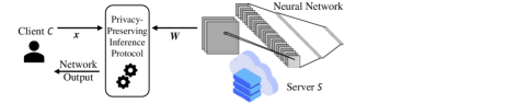
We consider the context of cryptographic inference (as shown in Figure 1) where $\mathcal{C}$ holds a private input $\bm{x}$ and $\mathcal{S}$ holds the neural network with proprietary model parameters $\bm{W}$. After the inference, $\mathcal{C}$ learns two pieces of information: the network architecture (such as the number, types and dimensions of involved functions) and the network output, while $\mathcal{S}$ learns nothing. The neural network processes $\bm{x}$ through a sequence of linear and nonlinear functions to finally classify $\bm{x}$ into one of the potential classes. Specifically, we target at the widely-applied Convolutional Neural Network (CNN) and describe its included functions as follows.

Convolution (Conv). The Conv operates between a three-dimension input $\bm{a}\in\mathcal{R}^{c_{i}\times{h_{i}}\times{w_{i}}}$ (the $\mathcal{R}$ is defined in Sec. 2.3.1) and the kernel $\textbf{K}\in\mathcal{R}^{c_{o}\times{c_{i}}\times{f_{h}}\times{f_{w}}}$ with a stride $s\in\mathbb{N}^{+}$ where $c_{i}$ and $c_{o}$ are the number of input and output channels, $h_{i}$ and $w_{i}$ are the height and width of each two-dimension input channel, and $f_{h}$ and $f_{w}$ are the height and width (which are always equal) of each two-dimension filter of K. The output is a three-dimension matrix $\bm{y}=\textsf{Conv}(\bm{a},\textbf{K})\in\mathcal{R}^{c_{o}\times{h_{i}^{\prime}}\times{w_{i}^{\prime}}}$ where $h_{i}^{\prime}=\left\lceil\frac{h_{i}}{s}\right\rceil$ and $w_{i}^{\prime}=\left\lceil\frac{w_{i}}{s}\right\rceil$ are the height and width of the two-dimension output channel. Such strided convolution is mathematically expressed as

$$\bm{y}_{\alpha,\beta,\gamma}=\sum_{\lambda\in{[c_{i}]}}\sum_{\ell_{1},\ell_{2}\in\bm{\delta}}\bm{a}_{\lambda,s\beta+\ell_{1},s\gamma+\ell_{2}}\textbf{K}_{\alpha,\lambda,\ell_{1}+\Delta,\ell_{2}+\Delta}$$

where $\bm{\delta}=\mathbb{Z}\cap[-\frac{f_{h}-1}{2},\frac{f_{h}-1}{2}]$, $\Delta=\frac{f_{h}-1}{2}$ and $\bm{a}_{\lambda,s\beta+\ell_{1},s\gamma+\ell_{2}}=0$ if $s\beta+\ell_{1}<0$ or $s\gamma+\ell_{2}<0$. The summing process in the cryptographic inference inevitably introduces a series of expensive rotations which limits the inference efficiency, a carefully designed matrix encoding is proposed in this work, together with the joint computation with the nonlinear function, which efficiently removes all the expensive rotations (see Sec. 3).

Dot Product (Dot). The input to the dot product is a $n_{i}$-sized vector $\bm{a}\in\mathcal{R}^{n_{i}}$ and the output is the $n_{o}$-sized vector $\bm{y}=\textsf{Dot}(\textbf{W},\bm{a})\in\mathcal{R}^{n_{o}}$ where

$$\bm{y}_{j}=\sum_{\lambda\in{[n_{i}]}}\textbf{W}_{j,\lambda}\bm{a}_{\lambda}$$ (1)

and $\textbf{W}\in\mathcal{R}^{n_{o}\times{n_{i}}}$. As the dot product and convolution are both intrinsically weighted sums, we treat dot product similarly with convolution in the cryptographic inference where the proposed matrix encoding for Dot, along with the joint computation with the nonlinear function (see Sec. 3), efficiently eliminates all the expensive rotations.

Batch Normalization (BN). In the neural network inference, the BN scales and shifts each two-dimension input channel by a constant $\bm{\mu}_{\beta}\in\mathcal{R}$ and $\bm{\theta}_{\beta}\in\mathcal{R}$, respectively, given the input $\bm{a}\in\mathcal{R}^{c_{i}\times{h_{i}}\times{w_{i}}}$. This operation is mathematically expressed as

$$\bm{a}_{\beta,:,:}\leftarrow\bm{\mu}_{\beta}\bm{a}_{\beta,:,:}+\bm{\theta}_{\beta}$$

As the BN always follows behind the convolution, we integrate it with the convolution (see Sec. 3), together with our joint computation with nonlinear function, to improve the efficiency for calculating the Conv+BN.

ReLU. For a value $a\in\mathcal{R}$, the ReLU is calculated as $\textsf{ReLU}(a)=a\cdot\textbf{1}\{a\}$. In the context of cryptographic inference, the multiplication between $a$ and $\textbf{1}\{a\}$ (denoted by $\textsf{DReLU}(a)$ thereafter) involves the multiplexing with noticeable communication rounds (e.g., about one third for OT-based communication rounds in [17]). In this work, we combine the ReLU computation with Conv (see Sec. 3) to totally relieve that cost.

Mean Pooling (MeanPool). Given the input $\bm{a}\in\mathcal{R}^{c_{i}\times{h_{i}}\times{w_{i}}}$, the MeanPool sums and averages the components in each $s_{\textsf{mp}}\times{s_{\textsf{mp}}}$ pooling window where $s_{\textsf{mp}}\in\mathbb{N}^{+}$, and returns all mean values as output. In this way, the output size becomes $c_{i}\times{\left\lceil\frac{h_{i}}{s_{\textsf{mp}}}\right\rceil}\times{\left\lceil\frac{w_{i}}{s_{\textsf{mp}}}\right\rceil}$. Since the MeanPool always appears between Conv and ReLU, we decouple its summing and averaging to ReLU and Conv (see Sec. 3) to utilize our joint computation block for a more efficient cryptographic inference.

Max Pooling (MaxPool). The MaxPool works similarly as MeanPool except that the returned value is the maximum in each $s_{\textsf{mxp}}\times{s_{\textsf{mxp}}}$ pooling window where $s_{\textsf{mxp}}\in\mathbb{N}^{+}$. The state-of-the-art framework deals with MaxPool in each $s_{\textsf{mxp}}\times{s_{\textsf{mxp}}}$ pooling window via $(s_{\textsf{mxp}}^{2}-1)$ sequential comparisons [17] and we further parallel this process by considering the independent nature of two comparisons among four values (see Sec. 3).

ArgMax. The ArgMax is usually the last function in a neural network to classify $\mathcal{C}$’s input to a potential class. ArgMax operates similarly as the MaxPool except that its pooling window embraces all values of the input and it finally returns the index of the maximum. The calculation of ArgMax is traditionally in a sequential manner [17], which is optimized in a similar way as MaxPool.

2.2 Threat Model

Our protocol involves two parties namely the client $\mathcal{C}$ and the server $\mathcal{S}$, and we follow in this work the static semi-honest security definition [38] for secure two-party computation.

Static Semi-Honest Security. There are two parties denoted by $\mathcal{C}$ and $\mathcal{S}$. Let $f_{\mathcal{C}}(\bm{x},\bm{W})$ and $f_{\mathcal{S}}(\bm{x},\bm{W}))$ be the output for $\mathcal{C}$ and $\mathcal{S}$ in the ideal functionality $\mathcal{F}$, respectively, while $f(\bm{x},\bm{W})=(f_{\mathcal{C}}(\bm{x},\bm{W}),f_{\mathcal{S}}(\bm{x},\bm{W})))$ be the joint output. Let the view of $\mathcal{C}$ and $\mathcal{S}$ during an execution of $\Pi$ on inputs $(\bm{x},\bm{W})$ be $\textsf{view}_{\mathcal{C}}^{\Pi}(\bm{x},\bm{W})$ and $\textsf{view}_{\mathcal{S}}^{\Pi}(\bm{x},\bm{W})$ that consist of the private input $\bm{x}$ and model parameters $\bm{W}$, as well as the contents of internal random tap and the messages received at $\mathcal{C}$ and $\mathcal{S}$ during the execution, respectively. Similarly, $\textsf{output}_{\mathcal{C}}^{\Pi}(\bm{x},\bm{W})$ and $\textsf{output}_{\mathcal{S}}^{\Pi}(\bm{x},\bm{W})$ are the output of $\mathcal{C}$ and $\mathcal{S}$ during an execution of $\Pi$ on inputs $(\bm{x},\bm{W})$ and can be computed from the $\Pi$’s view. The joint output of both parties is $\textsf{output}^{\Pi}(\bm{x},\bm{W})=(\textsf{output}_{\mathcal{C}}^{\Pi}(\bm{x},\bm{W}),\textsf{output}_{\mathcal{S}}^{\Pi}(\bm{x},\bm{W}))$.

Definition 1. A protocol $\Pi$ securely computes $\mathcal{F}$ against static semi-honest adversaries $\mathcal{A}$ if there exist probabilistic polynomial-time (PPT) algorithms $\textsf{Sim}_{\mathcal{C}}$ and $\textsf{Sim}_{\mathcal{S}}$ such that

$$\{\textsf{Sim}_{\mathcal{C}}(\bm{x},f_{\mathcal{C}}(\bm{x},\bm{W})),f(\bm{x},\bm{W})\}\overset{\textsf{c}}{\equiv}\{\textsf{view}_{\mathcal{C}}^{\Pi}(\bm{x},\bm{W}),\textsf{output}^{\Pi}(\bm{x},\bm{W})\},$$

$$\{\textsf{Sim}_{\mathcal{S}}(\bm{W},f_{\mathcal{S}}(\bm{x},\bm{W})),f(\bm{x},\bm{W})\}\overset{\textsf{c}}{\equiv}\{\textsf{view}_{\mathcal{S}}^{\Pi}(\bm{x},\bm{W}),\textsf{output}^{\Pi}(\bm{x},\bm{W})\}.$$

The main ideal functionalities for our protocol are $\mathcal{F}_{\textsf{DReLU}}$ and $\mathcal{F}_{\textsf{ReConv}}$ as shown in Algorithm 3 and Algorithm 4, and we prove in Sec. 3.2.5 that our designed protocol $\Pi_{\textsf{ReConv}}^{\textrm{ring},p}$ presented in Algorithm 2 securely realizes $\mathcal{F}_{\textsf{ReConv}}$ in the $\{\mathcal{F}_{\textsf{DReLU}}\}$-hybrid model, in the presence of semi-honest adversaries. Furthermore, we do not defend against attacks, such as the API attacks [39, 40], which are based purely on the inference results and other orthogonal techniques, such as differential privacy [41, 42], can be utilized to provide more privacy guarantee [37].

2.3 Cryptographic Primitives

2.3.1 Packed Homomorphic Encryption (PHE). PHE is a primitive that supports various vector operations over encrypted data without decryption, and generates an encrypted result which matches the corresponding operations on plaintext [26, 27, 28]. Specifically, given a vector $\bm{x}=(x_{0},x_{1},\dots,x_{n-1})\in\mathcal{R}^{n}$ over a ring $\mathcal{R}=\mathbb{Z}_{p}=\mathbb{Z}\cap(-p/2,p/2]$, it is encrypted into a ciphertext ct${}_{\bm{x}}^{\textsf{pk}_{\mathcal{C}}}=$ Enc${}^{\textsf{pk}_{\mathcal{C}}}(\bm{x})$ where pk_C denotes the public key of the client $\mathcal{C}$ and we thereafter use ct${}_{\bm{x}}^{{\mathcal{C}}}=$ Enc${}^{{\mathcal{C}}}(\bm{x})$ for brevity. Similar logic is applied for the ciphertext ct${}_{\bm{x}}^{{\mathcal{S}}}=$ Enc${}^{{\mathcal{S}}}(\bm{x})$ where $\bm{x}$ is encrypted by the public key of the server $\mathcal{S}$. The correctness of PHE is firstly guaranteed by a decryption process such that $\bm{x}=$ Dec${}^{\textsf{sk}_{\star}}(\textsf{ct}_{\bm{x}}^{\star})$ where ${\star}\in\{\mathcal{C},\mathcal{S}\}$, $\textsf{sk}_{\star}$ is the secret key of either $\mathcal{C}$ or $\mathcal{S}$, and Dec${}^{\star}()$ is used henceforth to simplify the notation for decryption. Second, the PHE system can securely evaluate an arithmetic circuit consisting of addition and multiplication gates by leveraging the following operations where $\bm{u}=(u_{0},\dots,u_{n-1})$ (resp. $\bm{v}=(v_{0},\dots,v_{n-1})$) $\in\mathcal{R}^{n}$, and $``+"$ (resp. $``-"$ and $``\cdot"$) is the component-wise addition (resp. subtraction and multiplication).

• Homomorphic addition $(\oplus)$ and subtraction $(\ominus)$: Dec${}^{\star}(\textsf{ct}_{\bm{u}}^{\star}$ $\oplus$ $\textsf{ct}_{\bm{v}}^{\star})=\bm{u}+\bm{v}$ (resp. Dec${}^{\star}(\textsf{ct}_{\bm{u}}^{\star}\oplus{\bm{v}})=\bm{u}+\bm{v}$) and Dec${}^{\star}(\textsf{ct}_{\bm{u}}^{\star}\ominus\textsf{ct}_{\bm{v}}^{\star})=\bm{u}-\bm{v}$ (resp. Dec${}^{\star}(\textsf{ct}_{\bm{u}}^{\star}\ominus{\bm{v}})=\bm{u}-\bm{v}$).

• Homomorphic multiplication $(\otimes)$: Dec${}^{\star}(\textsf{ct}_{\bm{u}}^{\star}\otimes\textsf{ct}_{\bm{v}}^{\star})=\bm{u}\cdot\bm{v}$ (resp. Dec${}^{\star}(\textsf{ct}_{\bm{u}}^{\star}\otimes{\bm{v}})=\bm{u}\cdot\bm{v}$).

• Homomorphic rotation (Rot): Dec${}^{\star}(\textsf{Rot}(\textsf{ct}_{\bm{u}}^{\star};\ell))=\bm{u}_{\ell}$ where $\bm{u}_{\ell}=\rho(\bm{u};\ell)=(u_{\ell},\dots,u_{n-1},u_{0},\dots,u_{\ell-1}$ $)$ and $\ell\in[n]$. Note that a rotation by $(-\ell)$ is the same as a rotation by $(n-\ell)$.

Given the above four operations, the runtime complexity of Rot is significantly larger than that of $\oplus$, $\ominus$ and $\otimes$ [37, 24]. Meanwhile, the runtime complexity of homomorphic multiplication between two ciphertext namely $\textsf{ct}_{\bm{u}}^{\star}$ $\otimes$ $\textsf{ct}_{\bm{v}}^{\star}$ is also larger than that of homomorphic multiplication between one ciphertext and one plaintext namely $\textsf{ct}_{\bm{u}}^{\star}$ $\otimes$ ${\bm{v}}$. While the neural network is composed of a stack of linear and nonlinear functions, the PHE is preferably utilized to calculate the linear functions such as Dot and Conv in the privacy-preserving neural networks, due to its intrinsic support for linear arithmetic computation [25]. Such computation process involves calling aforementioned PHE operations to get the encrypted output of linear function, which is then shared between $\mathcal{C}$ and $\mathcal{S}$ to serve as the input for computing next function, and this compute-and-share logic for the output of linear function is undoubtedly adopted in the state-of-the-art privacy-preserving frameworks [13, 16].

Unfortunately, this compute-and-share process requires a series of expensive Rot due to the needed summing in linear functions [13], and the PHE based linear calculation dominates the overall cost of neural model computation [18]. Therefore it makes the rotation elimination a significant and challenging task to achieve the next-stage boost towards computation efficiency. In this work, we jointly consider the computation for both linear and nonlinear functions, which enables us to feed the specifically- formed PHE intermediates from the linear function to the computation for the subsequent nonlinear function. Such joint design, rather than traditionally separate computation for each function output, contributes to efficiently eliminate all Rot in the entire process of cryptographic inference.

2.3.2 Oblivious Transfer (OT). In this work, we rely on OT to compute the comparison-based nonlinear functions such as ReLU, MaxPool and ArgMax. Specifically, in the 1-out-of-$k$ OT, $(\mathop{}_{1}^{k})$-OT_ℓ, the sender inputs $k$ $\ell$-length strings $m_{0},\dots,m_{k-1}$, and the receiver’s input is a value $i\in[k]$. The receiver gets $m_{i}$ after the OT functionality while the sender obtains nothing [43]. The state-of-the-art computation for a comparison-based nonlinear function mainly involves the OT-based DReLU functionality along with the OT-based multiplexer (Mux) to get the corresponding shares of such function output, which act as the input to compute next function [17]. While such process has relatively light computation and transmission load, the Mux accounts for nearly one third of the total communication rounds [17], which hinders the further optimization towards overall efficiency. In this paper, we totally remove the required Mux by a joint computation for both nonlinear and subsequent (linear) functions. Instead of getting the output shares with Mux, our design directly utilizes the nonlinear intermediates (e.g., DReLU) to generate the input of subsequent function.

2.3.3 Secret Sharing (SS). The additive SS over the ring $\mathcal{R}=\mathbb{Z}_{p}$ is adopted in this paper to form the output shares of linear or nonlinear functions, which serve as the input to compute next function. Here $p$ is either the plaintext modulus determined by the PHE for the linear functions or two for the boolean computation of nonlinear functions. Specifically, the SS algorithm $\textsf{Shr}(x)=(\langle x\rangle^{\mathcal{C}}_{p},\langle x\rangle^{\mathcal{S}}_{p})$ inputs an element $x$ in $\mathbb{Z}_{p}$ and generates shares of $x$, $\langle x\rangle^{\mathcal{C}}_{p}$ and $\langle x\rangle^{\mathcal{S}}_{p}$, over $\mathbb{Z}_{p}$. The shares are randomly sampled in $\mathbb{Z}_{p}$ such that $\langle x\rangle^{\mathcal{C}}_{p}\boxplus\langle x\rangle^{\mathcal{S}}_{p}=x$ where $``\boxplus"$ is the addition over $\mathbb{Z}_{p}$ and we similarly denote $``\boxminus"$ and $``\boxdot"$ as the subtraction and multiplication over $\mathbb{Z}_{p}$. Furthermore, we denote the reconstruction of $x$ as $\textsf{Rec}(\langle x\rangle^{\mathcal{C}}_{p},\langle x\rangle^{\mathcal{S}}_{p})=\langle x\rangle^{\mathcal{C}}_{p}\boxplus\langle x\rangle^{\mathcal{S}}_{p}=x$. Conventional $\textsf{Shr}(x)$ functionality in the state-of-the-art frameworks needs to exactly obtain the encrypted $x$ with massive amount of either computation-intensive Rot for a linear function or round-intensive Mux for the nonlinear function [17]. By carefully sharing specific intermediates in the process of computing adjacent functions, we efficiently eliminate all Rot and Mux in the cryptographic inference.

Input: $\langle{\bm{a}}\rangle_{p}^{\mathcal{C}}$ from $\mathcal{C}$, and $\langle{\bm{a}}\rangle_{p}^{\mathcal{S}}$, $\textrm{{K}}\in\mathbb{Z}_{p}^{c_{o}\times{c_{i}}\times{f_{h}}\times{f_{w}}}$ fro- m $\mathcal{S}$ where $\bm{a}$ $\in{\mathbb{Z}_{p}^{c_{i}\times{h_{i}}\times{w_{i}}}}$.

Output: $\mathcal{C}$ and $\mathcal{S}$ get $\langle{\bm{y}}\rangle_{p}^{\mathcal{C}}$ and $\langle{\bm{y}}\rangle_{p}^{\mathcal{S}}$, respectively, wh -ere $\bm{y}=\textsf{Conv}(\textsf{ReLU}(\bm{a}),\textrm{{K}})\in{\mathbb{Z}_{p}^{c_{o}\times{h_{i}^{\prime}}\times{w_{i}^{\prime}}}}$.

/* get shares of $\bar{\bm{a}}=\textsf{ReLU}(\bm{a})$ */

1 $\mathcal{S}$ gets $\langle{\hat{\bm{a}}}\rangle_{2}^{\mathcal{S}}$ $\scriptstyle\overset{\$}{\leftarrow}$ $\mathbb{Z}_{2}^{c_{i}\times{h_{i}}\times{w_{i}}}$.

2 $\mathcal{C}$ interacts with $\mathcal{S}$ based on OT to obtain $\langle{\hat{\bm{a}}}\rangle_{2}^{\mathcal{C}}$ where $\textsf{Rec}($ $\langle{\hat{\bm{a}}}\rangle_{2}^{\mathcal{C}},\langle{\hat{\bm{a}}}\rangle_{2}^{\mathcal{S}})=\hat{\bm{a}}=\textsf{DReLU}(\bm{a})\in{\mathbb{Z}_{2}^{c_{i}\times{h_{i}}\times{w_{i}}}}$.

3 $\mathcal{C}$ and $\mathcal{S}$ compute the $\textsf{Mux}(\bm{a},\hat{\bm{a}})=\bar{\bm{a}}=\textsf{ReLU}(\bm{a})$ to- gether, and get $\langle{\bar{\bm{a}}}\rangle_{p}^{\mathcal{C}}$ and $\langle{\bar{\bm{a}}}\rangle_{p}^{\mathcal{S}}$ where $\textsf{Rec}(\langle{\bar{\bm{a}}}\rangle_{p}^{\mathcal{C}},\langle{\bar{\bm{a}}}\rangle_{p}^{\mathcal{S}}$ $)=\bar{\bm{a}}\in{\mathbb{Z}_{p}^{c_{i}\times{h_{i}}\times{w_{i}}}}$.

/* get shares of $\bm{y}=\textsf{Conv}(\textsf{ReLU}(\bm{a}),\textrm{{K}})$ */

4 $\mathcal{C}$ encrypts $\langle{\bar{\bm{a}}}\rangle_{p}^{\mathcal{C}}$ as Enc${}^{{\mathcal{C}}}({\langle{\bar{\bm{a}}}\rangle_{p}^{\mathcal{C}}})$ and sends it to $\mathcal{S}$.

5 $\mathcal{S}$ obtains Enc${}^{\mathcal{C}}(\bar{\bm{a}})=$ Enc${}^{{\mathcal{C}}}({\langle{\bar{\bm{a}}}\rangle_{p}^{\mathcal{C}}})$ $\oplus\langle{\bar{\bm{a}}}\rangle_{p}^{\mathcal{S}}$, and gets t- he $\textsf{Enc}^{\mathcal{C}}(\bm{y})$ based on Enc${}^{\mathcal{C}}(\bar{\bm{a}})$ and K through a seri- es of $\oplus$, $\otimes$ and Rot.

6 $\mathcal{S}$ samples $\langle{{\bm{y}}}\rangle_{p}^{\mathcal{S}}$ $\scriptstyle\overset{\$}{\leftarrow}$ $\mathbb{Z}_{p}^{c_{o}\times{h_{i}^{\prime}}\times{w_{i}^{\prime}}}$.

7 $\mathcal{S}$ computes the Enc${}^{\mathcal{C}}(\langle{\bm{y}}\rangle_{p}^{\mathcal{C}})=\textsf{Enc}^{\mathcal{C}}(\bm{y})\ominus\langle{{\bm{y}}}\rangle_{p}^{\mathcal{S}}$, whi- ch is then sent to $\mathcal{C}$.

8 $\mathcal{C}$ obtains $\langle{\bm{y}}\rangle_{p}^{\mathcal{C}}=\textsf{Dec}^{\mathcal{C}}(\textsf{Enc}^{\mathcal{C}}(\langle{\bm{y}}\rangle_{p}^{\mathcal{C}}))$.

Algorithm 1 Computation for ReLU and Conv, $\Pi_{\textsf{ReLU+Conv}}^{\textrm{ring},p}$

2.4 Linear and Nonlinear Transformations

Deevashwer Rathee et al. [17] have recently proposed efficient computation for linear and nonlinear functions $\Pi_{\textsf{ReLU+Conv}}^{\textrm{ring},p}$ as shown in Algorithm 1, which contributes to high-performance neural network inference. Specifically, there are mainly two parts in $\Pi_{\textsf{ReLU+Conv}}^{\textrm{ring},p}$ where the first one is to get the shares of ReLU based on the shares of previous function (as shown in the gray block of Algorithm 1), and the second one is to subsequently get the shares of Conv based on the shares of ReLU (as shown in the blue block of Algorithm 1). Here, the ReLU and Conv are analyzed together as they are always adjacent and serve as a repeatable module to form modern neural networks [3, 4]. Among the state-of-the-art frameworks [12, 13, 14, 15, 16, 17, 37, 36], the above two parts are independently optimized such that the efficiency-unfriendly Mux and Rot are extensively involved to produce shares of one function, which serve as the input to compute subsequent function. While it is definitely logical to address the efficiency optimization in function wise, we show in the following section that our design enables efficient elimination of Mux and Rot by jointly computing the ReLU and Conv. Generally, specific intermediates of ReLU are utilized to directly compute Conv and vice versa. Such joint computation produces a new building block $\Pi_{\textsf{ReConv}}^{\textrm{ring},p}$ that combines the computation process of stacked functions and achieves more efficient privacy-preserving neural network inference.

3 System Description

Figure 2: Overview of the proposed framework.

3.1 Overview

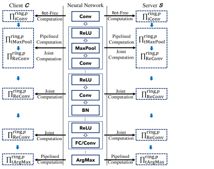
Figure 2 illustrates the overview of our proposed framework for cryptographic inference. Specifically, a neural network contains a stack of linear and nonlinear functions. As for a CNN, we group these functions into six blocks as: 1) the Conv block for $\mathcal{C}$’s input (i.e., the first function in the CNN); 2) the $\textsf{ReLU}+\textsf{MaxPool}+\textsf{Conv}$ block; 3) the $\textsf{ReLU}+\textsf{Conv}+\textsf{BN}$ block; 4) the $\textsf{ReLU}+\textsf{Conv}$ block; 5) the $\textsf{ReLU}+\textsf{FC}$ block; and 6) the ArgMax block for network’s output (i.e., the last function in the CNN). Such six blocks are able to construct many state-of-the-art CNN architectures such as VGG [3] and ResNet [4]. Compared with the function-wise optimization in existing schemes, which inevitably involves noticeable amount of expensive Rot and round-intensive Mux, we are motivated to jointly consider the computation process of functions in each block, aiming to efficiently eliminate the Rot and Mux, and thus to boost the performance of privacy-preserving inference.

As for the $\textsf{ReLU}+\textsf{Conv}$ block, we design the joint computation module $\Pi_{\textsf{ReConv}}^{\textrm{ring},p}$ (to be discussed in Sec. 3.2), which serves as the core component in our framework. The $\textsf{ReLU}+\textsf{MaxPool}+\textsf{Conv}$ block is converted into the combination of $\Pi_{\textsf{ReConv}}^{\textrm{ring},p}$ and our optimized module for MaxPool, $\Pi_{\textsf{tMaxPool}}^{\textrm{ring},p}$ (to be explained in Sec. 3.3). For neural network inference, the BN in $\textsf{ReLU}+\textsf{Conv}+\textsf{BN}$ block is integrated into the Conv, and it enables us to compute such transformed block by $\Pi_{\textsf{ReConv}}^{\textrm{ring},p}$. The calculation towards Conv block for $\mathcal{C}$’s input and $\textsf{ReLU}+\textsf{FC}$ block works similarly with $\Pi_{\textsf{ReConv}}^{\textrm{ring},p}$. Finally, the ArgMax block for network’s output is realized by our optimized module for ArgMax, $\Pi_{\textsf{tArgMax}}^{\textrm{ring},p}$ (to be marrated in Sec. 3.3). In the following, we first detail the construction of $\Pi_{\textsf{ReConv}}^{\textrm{ring},p}$ in Sec. 3.2 and then elaborate other optimizations in Sec. 3.3. Additionally, we follow the truncation strategy over $\mathbb{Z}_{p}$ [17] to deal with the floating-point computation.

3.2 The Joint Computation Module: $\Pi_{\textsf{ReConv}}^{\textrm{ring},p}$

For a lucid illustration, we begin with revisiting traditional calculation for the $\textsf{ReLU}+\textsf{Conv}$ block, where the PHE Triplet is proposed in Sec. 3.2.1 for Mux-free ReLU and our Matrix Encoding is described in Sec. 3.2.2 for Rot-free Conv. These two components form our joint computation module $\Pi_{\textsf{ReConv}}^{\textrm{ring},p}$. Different from the compute-and-share process in state-of-the-art function-wise computation, which exhaustively obtains encrypted output of current function and then shares that result to serve as the input for next function, $\Pi_{\textsf{ReConv}}^{\textrm{ring},p}$ shares specifically formed intermediates to finish computing $\textsf{ReLU}+\textsf{Conv}$ and we refer this methodology as share-in-the-middle logic (SIM). SIM enables efficient elimination of Rot and Mux, which are expensive in the state-of-the-art solutions. The overall process of $\Pi_{\textsf{ReConv}}^{\textrm{ring},p}$ is summarized in Sec. 3.2.3, which is followed by the corresponding complexity analysis in Sec. 3.2.4. The security of $\Pi_{\textsf{ReConv}}^{\textrm{ring},p}$ is justified in Sec. 3.2.5.

3.2.1 PHE Triplet Generation in ReLU. Recall in Algorithm 1 the traditional computation for $\textsf{ReLU}+\textsf{Conv}$, $\Pi_{\textsf{Relu+Conv}}^{\textrm{ring},p}$, where the input is the shares of previous function, $\langle{\bm{a}}\rangle_{p}^{\mathcal{C}}$ and $\langle{\bm{a}}\rangle_{p}^{\mathcal{S}}$. The conventional logic to compute ReLU includes the OT-based DReLU and subsequent Mux to obtain the output shares namely $\langle{\bar{\bm{a}}}\rangle_{p}^{\mathcal{C}}$ and $\langle{\bar{\bm{a}}}\rangle_{p}^{\mathcal{S}}$, which serve as the input of Conv (see the gray block in Algorithm 1). Since almost one third of the communication rounds are consumed by Mux to obtain the output shares of ReLU [17], we utilize the intermediates from DReLU to directly enable the subsequent Conv. This design efficiently removes the Mux in the process of $\textsf{ReLU}+\textsf{Conv}$. Specifically, given the shares of $\textsf{DReLU}(\bm{a})$, $\langle{\hat{\bm{a}}}\rangle_{2}^{\mathcal{C}}$ and $\langle{\hat{\bm{a}}}\rangle_{2}^{\mathcal{S}}$, the ReLU of $\bm{a}$ is computed according to

$$\textsf{ReLU}(\bm{a})=\textsf{DReLU}(\bm{a})\boxdot\bm{a}$$ (2)

$$=\underbrace{\{\langle{\hat{\bm{a}}}\rangle_{2}^{\mathcal{C}}\boxplus\langle{\hat{\bm{a}}}\rangle_{2}^{\mathcal{S}}\boxminus(\bm{2}\boxdot\langle{\hat{\bm{a}}}\rangle_{2}^{\mathcal{C}}\boxdot\langle{\hat{\bm{a}}}\rangle_{2}^{\mathcal{S}})\}}_{\leavevmode\hbox to8.5pt{\vbox to8.5pt{\pgfpicture\makeatletter\hbox{\hskip 4.25195pt\lower-4.25195pt\hbox to0.0pt{\pgfsys@beginscope\pgfsys@invoke{ }\definecolor{pgfstrokecolor}{rgb}{0,0,0}\pgfsys@color@rgb@stroke{0}{0}{0}\pgfsys@invoke{ }\pgfsys@color@rgb@fill{0}{0}{0}\pgfsys@invoke{ }\pgfsys@setlinewidth{0.4pt}\pgfsys@invoke{ }\nullfont\hbox to0.0pt{\pgfsys@beginscope\pgfsys@invoke{ }{{{}}\hbox{\hbox{{\pgfsys@beginscope\pgfsys@invoke{ }{{}{{{}}}{{}}{}{}{}{}{}{}{}{}{}{\pgfsys@moveto{4.25195pt}{0.0pt}\pgfsys@curveto{4.25195pt}{2.34831pt}{2.34831pt}{4.25195pt}{0.0pt}{4.25195pt}\pgfsys@curveto{-2.34831pt}{4.25195pt}{-4.25195pt}{2.34831pt}{-4.25195pt}{0.0pt}\pgfsys@curveto{-4.25195pt}{-2.34831pt}{-2.34831pt}{-4.25195pt}{0.0pt}{-4.25195pt}\pgfsys@curveto{2.34831pt}{-4.25195pt}{4.25195pt}{-2.34831pt}{4.25195pt}{0.0pt}\pgfsys@closepath\pgfsys@moveto{0.0pt}{0.0pt}\pgfsys@fill\pgfsys@invoke{ } }{{{{}}\pgfsys@beginscope\pgfsys@invoke{ }\pgfsys@transformcm{1.0}{0.0}{0.0}{1.0}{-1.75pt}{-2.25555pt}\pgfsys@invoke{ }\hbox{{\definecolor{pgfstrokecolor}{rgb}{0,0,0}\pgfsys@color@rgb@stroke{0}{0}{0}\pgfsys@invoke{ }\pgfsys@color@rgb@fill{0}{0}{0}\pgfsys@invoke{ }\hbox{\scriptsize{{\color[rgb]{1,1,1}\definecolor[named]{pgfstrokecolor}{rgb}{1,1,1}\pgfsys@color@gray@stroke{1}\pgfsys@color@gray@fill{1}1}}} }}\pgfsys@invoke{\lxSVG@closescope }\pgfsys@endscope}}} \pgfsys@invoke{\lxSVG@closescope }\pgfsys@endscope}}} } \pgfsys@invoke{\lxSVG@closescope }\pgfsys@endscope{{{}}}{}{}\hss}\pgfsys@discardpath\pgfsys@invoke{\lxSVG@closescope }\pgfsys@endscope\hss}}\lxSVG@closescope\endpgfpicture}}:\;\textrm{each}\;\textrm{operation}\;\textrm{is}\;\textrm{over}\;\mathbb{Z}_{p}^{c_{i}\times{h_{i}}\times{w_{i}}}}\boxdot(\langle{\bm{a}}\rangle_{p}^{\mathcal{C}}\boxplus\langle{\bm{a}}\rangle_{p}^{\mathcal{S}})$$ (3)

$$=\underbrace{(\langle{\bm{a}}\rangle_{p}^{\mathcal{C}}\boxdot\langle{\hat{\bm{a}}}\rangle_{2}^{\mathcal{C}}\boxminus{\color[rgb]{0,0,0}\definecolor[named]{pgfstrokecolor}{rgb}{0,0,0}\pgfsys@color@gray@stroke{0}\pgfsys@color@gray@fill{0}{\bm{r}^{\mathcal{C}}}})}_{\bm{h}_{1}}\boxplus\{\underbrace{\langle{\bm{a}}\rangle_{p}^{\mathcal{C}}\boxdot\{\bm{1}\boxminus(\bm{2}\boxdot\langle{\hat{\bm{a}}}\rangle_{2}^{\mathcal{C}})\}}_{\bm{h}_{2}}\boxdot\underbrace{{\color[rgb]{0,0,0}\definecolor[named]{pgfstrokecolor}{rgb}{0,0,0}\pgfsys@color@gray@stroke{0}\pgfsys@color@gray@fill{0}\langle{\hat{\bm{a}}}\rangle_{2}^{\mathcal{S}}}}_{{\color[rgb]{0,0,0}\definecolor[named]{pgfstrokecolor}{rgb}{0,0,0}\pgfsys@color@gray@stroke{0}\pgfsys@color@gray@fill{0}\bm{h}_{3}}}\}\boxplus$$

$$\{\underbrace{{\color[rgb]{0,0,0}\definecolor[named]{pgfstrokecolor}{rgb}{0,0,0}\pgfsys@color@gray@stroke{0}\pgfsys@color@gray@fill{0}\langle{\bm{a}}\rangle_{p}^{\mathcal{S}}\boxdot\{\bm{1}\boxminus(\bm{2}\boxdot\langle{\hat{\bm{a}}}\rangle_{2}^{\mathcal{S}})\}}}_{{\color[rgb]{0,0,0}\definecolor[named]{pgfstrokecolor}{rgb}{0,0,0}\pgfsys@color@gray@stroke{0}\pgfsys@color@gray@fill{0}\bm{h}_{4}}}\boxdot\underbrace{\langle{\hat{\bm{a}}}\rangle_{2}^{\mathcal{C}}}_{{\color[rgb]{0,0,0}\definecolor[named]{pgfstrokecolor}{rgb}{0,0,0}\pgfsys@color@gray@stroke{0}\pgfsys@color@gray@fill{0}\bm{h}_{5}}}\}\boxplus(\underbrace{\langle{\bm{a}}\rangle_{p}^{\mathcal{S}}\boxdot\langle{\hat{\bm{a}}}\rangle_{2}^{\mathcal{S}}}_{{\color[rgb]{0,0,0}\definecolor[named]{pgfstrokecolor}{rgb}{0,0,0}\pgfsys@color@gray@stroke{0}\pgfsys@color@gray@fill{0}\bm{h}_{6}}})\boxplus\underbrace{\color[rgb]{0,0,0}\definecolor[named]{pgfstrokecolor}{rgb}{0,0,0}\pgfsys@color@gray@stroke{0}\pgfsys@color@gray@fill{0}\bm{r}^{\mathcal{C}}}_{{\color[rgb]{0,0,0}\definecolor[named]{pgfstrokecolor}{rgb}{0,0,0}\pgfsys@color@gray@stroke{0}\pgfsys@color@gray@fill{0}\bm{h}_{7}}}.$$ (4)

Here $``\boxdot"$, $``\boxplus"$ and $``\boxminus"$ are element-wise plaintext multiplication, addition and subtraction, respectively. The item converts the shares of $\textsf{DReLU}(\bm{a})$ from $\mathbb{Z}_{2}^{c_{i}\times{h_{i}}\times{w_{i}}}$ to $\mathbb{Z}_{p}^{c_{i}\times{h_{i}}\times{w_{i}}}$. By rearranging and modifying the terms in Eq. (3), we finally get five to-be-added parts in Eq. (4) to obtain ReLU$(\bm{a})$: 1) the $\mathcal{C}$-computed $\bm{h}_{1}$ where $\bm{r}^{\mathcal{C}}{\scriptstyle\overset{\$}{\leftarrow}}\,\mathbb{Z}_{p}^{c_{i}\times{h_{i}}\times{w_{i}}}$; 2) the multiplication between $\mathcal{C}$-computed $\bm{h}_{2}$ and $\bm{h}_{3}$ namely $\langle{\hat{\bm{a}}}\rangle_{2}^{\mathcal{S}}$; 3) the multiplication between $\mathcal{S}$-computed $\bm{h}_{4}$ and $\bm{h}_{5}$ namely $\langle{\hat{\bm{a}}}\rangle_{2}^{\mathcal{C}}$; 4) the $\mathcal{S}$-computed $\bm{h}_{6}$; and 5) the $\bm{h}_{7}$ namely $\bm{r}^{\mathcal{C}}$. Given the input-independent nature of shares $\langle{\hat{\bm{a}}}\rangle_{2}^{\mathcal{S}}$, $\langle{{\bm{a}}}\rangle_{p}^{\mathcal{S}}$ and $\bm{r}^{\mathcal{C}}$ which are pregenerated by either $\mathcal{S}$ or $\mathcal{C}$ before the inference process, the $\bm{h}_{3}$, $\bm{h}_{4}$, $\bm{h}_{6}$ and $\bm{h}_{7}$ are pre-determined. Meanwhile, $\mathcal{C}$ would encrypt its share of $\textsf{ReLU}(\bm{a})$ and send it to $\mathcal{S}$ for obtaining encrypted $\textsf{ReLU}(\bm{a})$ and thus enabling the subsequent HE-based Conv. By carefully encrypting the pre-determined terms, without introducing Mux, we are able to make $\mathcal{S}$ obtain the encrypted input for Conv.

Therefore, we define the PHE triplet:

$$\{\textsf{ct}^{\mathcal{S}}_{\color[rgb]{0,0,0}\definecolor[named]{pgfstrokecolor}{rgb}{0,0,0}\pgfsys@color@gray@stroke{0}\pgfsys@color@gray@fill{0}\bm{h}_{3}},\textsf{ct}^{\mathcal{S}}_{\color[rgb]{0,0,0}\definecolor[named]{pgfstrokecolor}{rgb}{0,0,0}\pgfsys@color@gray@stroke{0}\pgfsys@color@gray@fill{0}\bm{h}_{4}},\textsf{ct}^{\mathcal{C}}_{\color[rgb]{0,0,0}\definecolor[named]{pgfstrokecolor}{rgb}{0,0,0}\pgfsys@color@gray@stroke{0}\pgfsys@color@gray@fill{0}\bm{h}_{7}}\}$$

where the first two terms are generated by $\mathcal{S}$ and sent to $\mathcal{C}$ while the last term is generated by $\mathcal{C}$ and sent to $\mathcal{S}$. Meanwhile, it is worth pointing out that each component in the above triplet is non-interactively formed and sent to either $\mathcal{C}$ or $\mathcal{S}$ offline. As such, $\mathcal{S}$ precomputes

$$\textsf{ct}_{\bm{h}_{8}}^{\mathcal{C}}=\bm{h}_{6}\oplus{\textsf{ct}^{\mathcal{C}}_{\color[rgb]{0,0,0}\definecolor[named]{pgfstrokecolor}{rgb}{0,0,0}\pgfsys@color@gray@stroke{0}\pgfsys@color@gray@fill{0}\bm{h}_{7}}}$$ (5)

while $\mathcal{C}$ obtains

$$\textsf{ct}_{\bm{h}_{9}}^{\mathcal{S}}=\bm{h}_{1}\oplus{(\bm{h}_{2}\otimes\textsf{ct}^{\mathcal{S}}_{\color[rgb]{0,0,0}\definecolor[named]{pgfstrokecolor}{rgb}{0,0,0}\pgfsys@color@gray@stroke{0}\pgfsys@color@gray@fill{0}\bm{h}_{3}})\oplus({\textsf{ct}^{\mathcal{S}}_{\color[rgb]{0,0,0}\definecolor[named]{pgfstrokecolor}{rgb}{0,0,0}\pgfsys@color@gray@stroke{0}\pgfsys@color@gray@fill{0}\bm{h}_{4}}\otimes{\bm{h}_{5}}})}$$ (6)

and sends it to $\mathcal{S}$ right after the DReLU computation. $\mathcal{S}$ then conducts the decryption as

$$\bm{h}_{9}=\textsf{Dec}^{\mathcal{S}}(\textsf{ct}_{\bm{h}_{9}}^{\mathcal{S}})=\bm{h}_{1}\boxplus{(\bm{h}_{2}\boxdot{\color[rgb]{0,0,0}\definecolor[named]{pgfstrokecolor}{rgb}{0,0,0}\pgfsys@color@gray@stroke{0}\pgfsys@color@gray@fill{0}\bm{h}_{3}})\boxplus({{\color[rgb]{0,0,0}\definecolor[named]{pgfstrokecolor}{rgb}{0,0,0}\pgfsys@color@gray@stroke{0}\pgfsys@color@gray@fill{0}\bm{h}_{4}}\boxdot{\bm{h}_{5}}})}.$$ (7)

It is obvious that $\textsf{ReLU}(\bm{a})=\bm{h}_{8}\boxplus\bm{h}_{9}$. Thus $\mathcal{S}$ obtains the $\mathcal{C}$-encrypted $\textsf{ReLU}(\bm{a})$ as

$$\textsf{ct}_{\bar{\bm{a}}}^{\mathcal{C}}=\textsf{ct}_{\bm{h}_{8}}^{\mathcal{C}}\oplus\bm{h}_{9},$$ (8)

which is utilized to compute Conv to be elaborated next. Note that the proposed PHE triplet enables us to eliminate the Mux and directly get the encrypted ReLU at $\mathcal{S}$ for computing the subsequent Conv, with only half a round after the DReLU. This helps to save all computation and communication cost for calling Mux.

3.2.2 Matrix Encoding for Conv. Based on the encrypted ReLU $\textsf{ct}_{\bar{\bm{a}}}^{\mathcal{C}}$ in Eq. (8), $\mathcal{S}$ is supposed to utilize its kernel K to compute the Conv (see the blue block in Algorithm 1). In other words, $\mathcal{S}$ should obtain Enc${}^{\mathcal{C}}(\bm{y})=\textsf{Conv}(\textsf{ct}_{\bar{\bm{a}}}^{\mathcal{C}},\textrm{{K}})$ and share it with $\mathcal{C}$. The state-of-the-art frameworks extensively call the PHE operations to get the encrypted output of Conv, which is then shared between $\mathcal{C}$ and $\mathcal{S}$ to compute the subsequent function. However, it inevitably involves a series of Rot due to the needed summing process [13]. We totally relieve the need for Rot via a carefully designed matrix encoding.

Our main idea lays in the observation that the dot product between a matrix and a vector in Eq. (1) can be viewed as the linear combination of all columns in that matrix. As such, if the $\textsf{ReLU}(\bm{a})$ and kernel K were respectively such matrix and vector, we could construct $\textsf{ct}_{\bar{\bm{a}}}^{\mathcal{C}}$ as a set of ciphertext each of which encrypts one column in $\textsf{ReLU}(\bm{a})$, and the Conv output, Enc${}^{\mathcal{C}}(\bm{y})$, could be obtained by $\mathcal{S}$ via only HE multiplication and addition. In the following, we describe in detail the feasibility of above conjecture for Rot-free Conv, and Sec. 3.2.4 shows the efficiency advantages of our design compared with the state-of-the-art solution.

Specifically, we first transform the Conv $\bm{y}=\textsf{Conv}(\bar{\bm{a}},\textbf{{K}})$ $\in\mathcal{R}^{c_{o}\times h_{i}^{\prime}\times{w_{i}^{\prime}}}$ into corresponding dot product $\tilde{\bm{y}}=\textsf{Dot}(\tilde{\bm{a}},\tilde{\textbf{{K}}})$ $\in\mathcal{R}^{h_{i}^{\prime}w_{i}^{\prime}\times{c_{o}}}$ based on the im2col operator [44]. Recall that $\bar{\bm{a}}\in\mathcal{R}^{c_{i}\times h_{i}\times w_{i}}$ and ${\textbf{K}}\in\mathcal{R}^{c_{o}\times c_{i}\times f_{h}\times f_{w}}$, they are then respectively converted into $\tilde{\bm{a}}\in\mathcal{R}^{h_{i}^{\prime}w_{i}^{\prime}\times{c_{i}f_{h}f_{w}}}$ and $\widetilde{\textbf{K}}\in\mathcal{R}^{c_{i}f_{h}f_{w}\times{c_{o}}}$ such that $\tilde{\bm{y}}_{\alpha,\beta}=\bm{y}_{\beta,\gamma,\eta}$ where $\alpha\in[h_{i}^{\prime}w_{i}^{\prime}]$, $\beta\in[c_{o}]$, $\gamma=\left\lfloor\frac{\alpha}{w_{i}^{\prime}}\right\rfloor$, $h_{i}^{\prime}=\left\lceil\frac{h_{i}}{s}\right\rceil$, $w_{i}^{\prime}=\left\lceil\frac{w_{i}}{s}\right\rceil$, $\eta=\alpha$ mod $w_{i}^{\prime}$. In other words, each $c_{i}f_{h}f_{w}$ elements along the first dimension of K forms one column in $\widetilde{\textbf{K}}$ while each $c_{i}f_{h}f_{w}$ values in $\bar{\bm{a}}$ that are weighted and summed for one number of $\bm{y}$ forms a row in $\tilde{\bm{a}}$. Thereafter, we denote the mapping from ${\bm{y}}$ to $\tilde{\bm{y}}$ as $\phi:\bm{y}\mapsto{\tilde{\bm{y}}}$. Note that the conversion towards $\bar{\bm{a}}$ is completed during the ReLU process which is computed in element wise and is independent with element locations. Meanwhile the conversion towards K is easily performed by $\mathcal{S}$ since it’s in plaintext. We also summarize the overall procedure in Sec. 3.2.3.

Recall that we are supposed to construct $\textsf{ct}_{\bar{\bm{a}}}^{\mathcal{C}}$ such that the computation for Enc${}^{\mathcal{C}}(\bm{y})$ doesn’t involve any Rot. Given $\tilde{\bm{a}}$, a matrix encoding is proposed which produces a set of ciphertext and enables Rot-free Conv. Concretely, we define the encoding mapping $\iota:\mathcal{R}^{h_{i}^{\prime}w_{i}^{\prime}\times{c_{i}f_{h}f_{w}}}\mapsto\mathcal{R}^{d\times{n}}$ by

$$\iota:\tilde{\bm{a}}\mapsto{\textbf{{A}}}$$

where $\textbf{A}_{j,\zeta}=\tilde{\bm{a}}_{\tau,\lambda}$, $\lambda=j\xi+\left\lfloor\frac{\zeta}{h_{i}^{\prime}w_{i}^{\prime}}\right\rfloor$, $j\in[d]$, $\zeta\in[n]$, $\xi=\left\lfloor\frac{n}{h_{i}^{\prime}w_{i}^{\prime}}\right\rfloor$, $d=\left\lceil\frac{c_{i}f_{h}f_{w}}{\xi}\right\rceil$, and $\tau=\zeta$ mod $h_{i}^{\prime}w_{i}^{\prime}$. In this way, $\iota$ maps $\xi$ columns of $\tilde{\bm{a}}$ into one row of A. Meanwhile, $\forall\beta\in[c_{o}]$, we have $\tilde{\bm{y}}_{:,\beta}=\sum_{\lambda}\tilde{\bm{a}}_{:,\lambda}\widetilde{\textbf{{K}}}_{\lambda,\beta}$, which means that the $\beta$-th output channel after Conv is the summation of all weighted columns in $\tilde{\bm{a}}$ namely the $\lambda$-th cloumn $\tilde{\bm{a}}_{:,\lambda}$ is multiplied with $\widetilde{\textbf{{K}}}_{\lambda,\beta}$. Therefore, $\forall\beta$, $\sum_{j}(\textbf{A}_{j,:}\boxdot\overline{\textbf{K}}_{j,\beta})\in\mathcal{R}^{n}$ contains $\xi$ finally summed columns derived from $\{\tilde{\bm{a}}_{:,\lambda}\tilde{\textbf{{K}}}_{\lambda,\beta}\}_{\lambda}$ where $\overline{\textbf{K}}_{j,\beta}\in\mathcal{R}^{n}=\{\widetilde{\textbf{{K}}}_{j\xi,\beta}\}^{h_{i}^{\prime}w_{i}^{\prime}}|\cdots|\{\widetilde{\textbf{{K}}}_{(j+1)\xi-1,\beta}\}^{h_{i}^{\prime}w_{i}^{\prime}}|\{0\}^{n-h_{i}^{\prime}w_{i}^{\prime}\xi}$ and note that $\widetilde{\textbf{{K}}}_{\varphi,\beta}=0$ if $\varphi\geq{c_{i}f_{h}f_{w}}$.

Based on the element-wise operation of $\sum_{j}(\textbf{A}_{j,:}\boxdot\overline{\textbf{K}}_{j,\beta})$, we are ready to obtain a Rot-free Conv. In particular, each $\textbf{A}_{j,:}$ is encrypted into the ciphertext $\textsf{ct}_{\textbf{A}_{j,:}}^{\mathcal{C}}$, then $\forall\beta$, we obtain a $\textsf{ct}_{\textbf{B}_{\beta}}^{\mathcal{C}}=\oplus_{j}(\textsf{ct}_{\textbf{A}_{j,:}}^{\mathcal{C}}\odot\overline{\textbf{K}}_{j,\beta})$ which encrypts $\xi$ finally summed columns derived from $\{\tilde{\bm{a}}_{:,\lambda}\tilde{\textbf{{K}}}_{\lambda,\beta}\}_{\lambda}$. Here $\textbf{B}_{\beta}\in\mathcal{R}^{n}=\sum_{j}({\textbf{A}_{j,:}}\boxdot\overline{\textbf{K}}_{j,\beta})$. Considering that $\textbf{B}_{\beta}$ contains all partial sums for $\tilde{\bm{y}}_{:,\beta}$ and $\{\textsf{ct}^{\mathcal{C}}_{\textbf{B}_{\beta}}\}_{\beta}$ are obtained by $\mathcal{S}$ without Rot, $\mathcal{S}$ then directly shares $\{\textsf{ct}^{\mathcal{C}}_{\textbf{B}_{\beta}}\}_{\beta}$ by $\{\textsf{ct}^{\mathcal{C}}_{\textbf{C}_{\beta}}=\textsf{ct}^{\mathcal{C}}_{\textbf{B}_{\beta}}\ominus{\bm{r}^{\mathcal{S}}_{\beta}}\}_{\beta}$ where $\textbf{C}_{\beta}\in\mathcal{R}^{n}=\textbf{B}_{\beta}\boxminus\bm{r}^{\mathcal{S}}_{\beta}$ and $\bm{r}^{\mathcal{S}}_{\beta}{\scriptstyle\overset{\$}{\leftarrow}}\,\mathbb{Z}_{p}^{n}$. Then $\mathcal{S}$ sends $\{\textsf{ct}^{\mathcal{C}}_{\textbf{C}_{\beta}}\}_{\beta}$ to $\mathcal{C}$, which decrypts $\{\textsf{ct}^{\mathcal{C}}_{\textbf{C}_{\beta}}\}_{\beta}$ into $\{\textsf{Dec}^{\mathcal{C}}(\textsf{ct}^{\mathcal{C}}_{\textbf{C}_{\beta}})=\textbf{C}_{\beta}\}_{\beta}$ and gets

$$\left\langle\bm{y}\right\rangle_{p}^{\mathcal{C}}=\phi^{-1}(\left\langle\tilde{\bm{y}}_{:,0}\right\rangle_{p}^{\mathcal{C}}|\left\langle\tilde{\bm{y}}_{:,1}\right\rangle_{p}^{\mathcal{C}}|\cdots|\left\langle\tilde{\bm{y}}_{:,c_{o}-1}\right\rangle_{p}^{\mathcal{C}})$$ (9)

where $\left\langle\tilde{\bm{y}}_{:,\beta}\right\rangle_{p}^{\mathcal{C}}=\{\boxplus_{\chi=0}^{\xi-1}\textbf{C}_{\beta,\{h_{i}^{\prime}w_{i}^{\prime}\chi:h_{i}^{\prime}w_{i}^{\prime}(\chi+1)\}}\}^{\top}$. Meanwhile, $\mathcal{S}$ computes

$$\left\langle\bm{y}\right\rangle_{p}^{\mathcal{S}}=\phi^{-1}(\left\langle\tilde{\bm{y}}_{:,0}\right\rangle_{p}^{\mathcal{S}}|\left\langle\tilde{\bm{y}}_{:,1}\right\rangle_{p}^{\mathcal{S}}|\cdots|\left\langle\tilde{\bm{y}}_{:,c_{o}-1}\right\rangle_{p}^{\mathcal{S}})$$ (10)

where $\left\langle\tilde{\bm{y}}_{:,\beta}\right\rangle_{p}^{\mathcal{S}}=\{\boxplus_{\chi=0}^{\xi-1}\bm{r}^{\mathcal{S}}_{\beta,\{h_{i}^{\prime}w_{i}^{\prime}\chi:h_{i}^{\prime}w_{i}^{\prime}(\chi+1)\}}\}^{\top}$. Here $\mathcal{S}$ is able to get $\left\langle\bm{y}\right\rangle_{p}^{\mathcal{S}}$ offline. As such, $\mathcal{C}$ and $\mathcal{S}$ respectively obtain their shares of Conv, which act as the input of subsequent function.

Input: $\langle{\bm{a}}\rangle_{p}^{\mathcal{C}}$ from $\mathcal{C}$, and $\langle{\bm{a}}\rangle_{p}^{\mathcal{S}}$, $\textrm{{K}}\in\mathbb{Z}_{p}^{c_{o}\times{c_{i}}\times{f_{h}}\times{f_{w}}}$ fr- om $\mathcal{S}$ where $\bm{a}$ $\in{\mathbb{Z}_{p}^{c_{i}\times{h_{i}}\times{w_{i}}}}$.

Output: $\mathcal{C}$ and $\mathcal{S}$ get $\langle{\bm{y}}\rangle_{p}^{\mathcal{C}}$ and $\langle{\bm{y}}\rangle_{p}^{\mathcal{S}}$, respectively, w- here $\bm{y}=\textsf{Conv}(\textsf{ReLU}(\bm{a}),\textrm{{K}})\in{\mathbb{Z}_{p}^{c_{o}\times{h_{i}^{\prime}}\times{w_{i}^{\prime}}}}$.

/* offline computation */

1 $\mathcal{C}$ gets $\bm{r}^{\mathcal{C}}$ $\scriptstyle\overset{\$}{\leftarrow}\,\mathbb{Z}_{p}^{c_{i}\times{h_{i}}\times{w_{i}}}$, maps $\bm{h}_{7}$ to H based on $\iota$ whi- ch has the same structure as A (mapped from $\bar{\bm{a}}$), an- d encrypts H as $\{\textsf{ct}_{\textbf{H}_{j,:}}^{\mathcal{C}}\}_{j\in[d]}$ which are sent to $\mathcal{S}$.

2 $\mathcal{S}$ maps K to $\overline{\textbf{K}}$, generates $\langle{\hat{\bm{a}}}\rangle_{2}^{\mathcal{S}}$ $\scriptstyle\overset{\$}{\leftarrow}\,\mathbb{Z}_{2}^{c_{i}\times{h_{i}}\times{w_{i}}}$ and $\{\bm{r}^{\mathcal{S}}_{\beta}$ ${\scriptstyle\overset{\$}{\leftarrow}}\,\mathbb{Z}_{p}^{n}\}_{\beta}$, maps $\bm{h}_{6}$ to $\widehat{\textbf{H}}$ based on $\iota$ which has the sa- me structure as A, maps $\bm{h}_{3}$ and $\bm{h}_{4}$ to $\overline{\textbf{H}}$ and $\widetilde{\textbf{H}}$, res- pectively, where $\psi:\bm{h}_{3}\mapsto$ $\overline{\textbf{H}}$. Here $\overline{\textbf{H}}_{\nu,:}$ places each $n$ elements of $\bm{h}_{3}$ in a row where $\nu\in[\sigma=\left\lceil\frac{c_{i}h_{i}w_{i}}{n}\right\rceil]$, and $\widetilde{\textbf{H}}$ has the same structure as $\overline{\textbf{H}}$. $\mathcal{S}$ also encrypts $\overline{\textbf{H}}$ and $\widetilde{\textbf{H}}$ to $\{\textsf{ct}_{\overline{\textbf{H}}_{\nu,:}}^{\mathcal{S}}\}_{\nu}$ and $\{\textsf{ct}_{\widetilde{\textbf{H}}_{\nu,:}}^{\mathcal{S}}\}_{\nu}$ which are then s- ent to $\mathcal{C}$, obtains the $\left\langle\bm{y}\right\rangle_{p}^{\mathcal{S}}$ by Eq. 10, and then comp- utes $\{\textsf{ct}_{\widecheck{\textbf{H}}_{j,:}}^{\mathcal{C}}=\widehat{\textbf{H}}_{j,:}\oplus\textsf{ct}_{{\textbf{H}}_{j,:}}^{\mathcal{C}}\}_{j}$ based on Eq. 5.

/* $\mathcal{C}$’s share of $\bm{y}=\textsf{Conv}(\textsf{ReLU}(\bm{a}),\textrm{{K}})$ */

3 $\mathcal{C}$ interacts with $\mathcal{S}$ based on OT to obtain $\langle{\hat{\bm{a}}}\rangle_{2}^{\mathcal{C}}$ where $\textsf{Rec}($ $\langle{\hat{\bm{a}}}\rangle_{2}^{\mathcal{C}},\langle{\hat{\bm{a}}}\rangle_{2}^{\mathcal{S}})=\hat{\bm{a}}=\textsf{DReLU}(\bm{a})\in{\mathbb{Z}_{2}^{c_{i}\times{h_{i}}\times{w_{i}}}}$.

4 $\mathcal{C}$ maps $\bm{h}_{1}$, $\bm{h}_{2}$ and $\bm{h}_{5}$ to $\breve{\textbf{H}}$, $\ddot{\textbf{H}}$ and $\dot{\textbf{H}}$ based on $\psi$, re- spectively, which all have the same structures as $\overline{\textbf{H}}$, a -nd then computes $\{\textsf{ct}_{\acute{\textbf{H}}_{\nu,:}}^{\mathcal{S}}$= $\breve{\textbf{H}}_{\nu,:}\oplus(\ddot{\textbf{H}}_{\nu,:}\otimes{\textsf{ct}_{\overline{\textbf{H}}_{\nu,:}}^{\mathcal{S}}})\oplus($ $\textsf{ct}_{\widetilde{\textbf{H}}_{\nu,:}}^{\mathcal{S}}\otimes\dot{\textbf{H}}_{\nu,:})\}_{\nu}$ based on Eq. 6, which are sent to $\mathcal{S}$.

5 $\mathcal{S}$ decrypts $\{\textsf{ct}_{\acute{\textbf{H}}_{\nu,:}}^{\mathcal{S}}\}_{\nu}$ to $\{\acute{\textbf{H}}_{\nu,:}=\textsf{Dec}^{\mathcal{S}}(\textsf{ct}_{\acute{\textbf{H}}_{\nu,:}}^{\mathcal{S}})\}_{\nu}$ based on Eq. 7, gets $\bm{h}_{9}=\psi^{-1}(\acute{\textbf{H}})$, maps $\bm{h}_{9}$ to $\grave{\textbf{H}}$ based on $\iota$, computes $\{\textsf{ct}_{\textbf{A}_{j,:}}^{\mathcal{C}}$= $\textsf{ct}_{\widecheck{\textbf{H}}_{j,:}}^{\mathcal{C}}\oplus\grave{\textbf{H}}_{j,:}\}_{j}$ based on Eq. 8, ob -tains $\{\textsf{ct}^{\mathcal{C}}_{\textbf{B}_{\beta}}\}_{\beta\in[c_{o}]}$ and gets $\{\textsf{ct}^{\mathcal{C}}_{\textbf{C}_{\beta}}\}_{\beta}$ which are sent t -o $\mathcal{C}$.

$\mathcal{C}$ decrypts $\{\textsf{ct}^{\mathcal{C}}_{\textbf{C}_{\beta}}\}_{\beta}$ to $\{\textbf{C}_{\beta}\}_{\beta}$, and gets $\left\langle\bm{y}\right\rangle_{p}^{\mathcal{C}}$ based on Eq. 9.

Algorithm 2 Joint computation of ReLU and Conv, $\Pi_{\textsf{ReConv}}^{\textrm{ring},p}$

3.2.3 Putting Things Together. With the proposed PHE triplet in ReLU and the matrix encoding for Conv, the Mux in ReLU and the Rot in Conv are totally eliminated, which forms our building block $\Pi_{\textsf{ReConv}}^{\textrm{ring},p}$ to compute consecutive ReLU and Conv. The complexity analysis to be elaborated in Sec. 3.2.4 demonstrates the numerical advantages of $\Pi_{\textsf{ReConv}}^{\textrm{ring},p}$ compared with the state-of-the-art function-wise design [17]. Algorithm 2 summaries the joint computation process. Specifically, we have an offline phase for precomputation and an online phase for getting $\langle{\bm{y}}\rangle_{p}^{\mathcal{C}}$ based on the shares of DReLU. Since the dimension of $\bar{\bm{a}}$ is the same as the ones of seven items in Eq. (4), the structures of $\bm{h}_{1}$ to $\bm{h}_{7}$ are correspondingly tuned to transform $\textsf{ct}_{\bar{\bm{a}}}^{\mathcal{C}}$ to $\{\textsf{ct}_{\textbf{{A}}_{j,:}}^{\mathcal{C}}\}_{j}$.

Concretely, the structures of $\bm{h}_{6}$ and $\bm{h}_{7}$ are mapped to the one of A. Meanwhile, as $\bm{h}_{9}$ is homomorphically obtained by $\mathcal{C}$ based on Eq. 6 and is then decrypted by $\mathcal{S}$ based on Eq. 7, the structures of $\bm{h}_{1}$ to $\bm{h}_{5}$ can be as tight as possible (see the mapping $\psi$ in Algorithm 2) to enable minimal calls of PHE operations at both $\mathcal{S}$ and $\mathcal{C}$. Furthermore, the mapped $\bm{h}_{9}$ at $\mathcal{S}$ has the same structure as A, which enables $\mathcal{S}$ to compute $\{\textsf{ct}_{\textbf{{A}}_{j,:}}^{\mathcal{C}}\}_{j}$ based on Eq. 8. After that, $\mathcal{S}$ gets $\{\textsf{ct}^{\mathcal{C}}_{\textbf{C}_{\beta}}\}_{\beta}$ which are later decrypted by $\mathcal{C}$ as $\{\textbf{C}_{\beta}\}_{\beta}$. $\mathcal{C}$ finally gets $\left\langle\bm{y}\right\rangle_{p}^{\mathcal{C}}$ based on Eq. 9. The offline computation mainly involves the generation of our PHE triplet whose non-interactive and input-independent nature relieves the necessary synchronization required in other state-of-the-art offline processes [12, 16]. After $\Pi_{\textsf{ReConv}}^{\textrm{ring},p}$, the shares of Conv $\bm{y}$ act as the input of subsequent function. Note that the bias $\bm{b}\in\mathcal{R}^{c_{o}}$ in the Conv is combined with $\{\bm{r}^{\mathcal{S}}_{\beta}\}_{\beta}$ such that

$$\left\langle\tilde{\bm{y}}_{:,\beta}\right\rangle_{p}^{\mathcal{S}}=\{\boxplus_{\chi=0}^{\xi-1}\bm{r}^{\mathcal{S}}_{\beta,(h_{i}^{\prime}w_{i}^{\prime}\chi:h_{i}^{\prime}w_{i}^{\prime}(\chi+1))}\}^{\top}\boxplus\bm{b}_{\beta}.$$

Furthermore, our joint computation block is easily adapted for the $\textsf{ReLU}+\textsf{FC}$ block. Concretely, the $\bar{\bm{a}}=\textsf{ReLU}(\bm{a})$ becomes an $n_{i}$-size vector and the mapping $\iota$ becomes

$$\iota:\bar{\bm{a}}\mapsto{\textbf{A}}$$

where $\textbf{A}\in\mathcal{R}^{{n}}=\{\bar{\bm{a}}\}^{\xi}|\{0\}^{n-n_{i}\xi}$. The weight matrix $\textbf{W}\in\mathcal{R}^{n_{o}\times{n_{i}}}$ is transformed to $\bar{\textbf{W}}\in\mathcal{R}^{d_{1}\times{n}}$ where $d_{1}\in{[\left\lceil\frac{n_{o}}{\xi}\right\rceil]}$, $\xi=\left\lfloor\frac{n}{n_{i}}\right\rfloor$ and $\bar{\textbf{W}}_{j,:}=\textbf{W}_{j\xi,:}|\cdots|\textbf{W}_{(j+1)\xi-1,:}|\{0\}^{n-n_{i}\xi}$, $j\in[d_{1}]$, $\textbf{W}_{\phi,:}=\{0\}^{n_{i}}$ if $\phi\geq{n_{o}}$. In this way, the $\textsf{ct}^{\mathcal{C}}_{\bar{\bm{a}}}$ obtained by $\mathcal{S}$, based on Eq. 8, turns out to be $\textsf{ct}^{\mathcal{C}}_{\textbf{A}}$ that encrypts $\xi$ copies of $\bar{\bm{a}}$ and the ciphertext $\textsf{ct}^{\mathcal{C}}_{\textbf{B}_{j}}=\textsf{ct}^{\mathcal{C}}_{\textbf{A}}\otimes{\bar{\textbf{W}}_{j,:}}$ contains all partial sums of $j\xi$-th to $(j\xi+\xi-1)$-th components in $\bm{y}=\textsf{Dot}(\textbf{W},\bar{\bm{a}})\in\mathcal{R}^{n_{o}}$. Without introducing the Rot, $\mathcal{S}$ shares $\{\textsf{ct}^{\mathcal{C}}_{\textbf{B}_{j}}\}_{j}$ by $\{\textsf{ct}^{\mathcal{C}}_{\textbf{C}_{j}}=\textsf{ct}^{\mathcal{C}}_{\textbf{B}_{j}}\ominus{\bm{r}^{\mathcal{S}}_{j}}\}_{j}$ and sends $\{\textsf{ct}^{\mathcal{C}}_{\textbf{C}_{j}}\}_{j}$ to $\mathcal{C}$, which decrypts $\{\textsf{ct}^{\mathcal{C}}_{\textbf{C}_{j}}\}_{j}$ into $\{\textsf{Dec}^{\mathcal{C}}(\textsf{ct}^{\mathcal{C}}_{\textbf{C}_{j}})=\textbf{C}_{j}\}_{j}$ and gets

$$\left\langle\bm{y}\right\rangle_{p}^{\mathcal{C}}=\left\langle{\bm{y}}_{0}\right\rangle_{p}^{\mathcal{C}}|\left\langle{\bm{y}}_{1}\right\rangle_{p}^{\mathcal{C}}|\cdots|\left\langle{\bm{y}}_{n_{o}-1}\right\rangle_{p}^{\mathcal{C}}$$ (11)

where $\left\langle{\bm{y}}_{\beta\in[n_{o}]}\right\rangle_{p}^{\mathcal{C}}=\boxplus_{\chi=0}^{n_{i}-1}\textbf{C}_{\tau,n_{i}\lambda+\chi}$, $\tau=\left\lfloor\frac{\beta}{\xi}\right\rfloor$, $\lambda=\beta\;\textrm{mod}\;\xi$. Meanwhile, $\mathcal{S}$ computes

$$\left\langle\bm{y}\right\rangle_{p}^{\mathcal{S}}=\left\langle{\bm{y}}_{0}\right\rangle_{p}^{\mathcal{S}}|\left\langle{\bm{y}}_{1}\right\rangle_{p}^{\mathcal{S}}|\cdots|\left\langle{\bm{y}}_{n_{o}-1}\right\rangle_{p}^{\mathcal{S}}$$ (12)

in offline and here $\left\langle{\bm{y}}_{\beta}\right\rangle_{p}^{\mathcal{S}}=\boxplus_{\chi=0}^{n_{i}-1}\bm{r}^{\mathcal{S}}_{\tau,n_{i}\lambda+\chi}$. Similar with Conv, the bias $\bm{b}\in\mathcal{R}^{n_{o}}$ is combined with $\{\bm{r}^{\mathcal{S}}_{j}\}_{j}$ such that

$$\left\langle{\bm{y}}_{\beta}\right\rangle_{p}^{\mathcal{S}}=\{\boxplus_{\chi=0}^{n_{i}-1}\bm{r}^{\mathcal{S}}_{\tau,n_{i}\lambda+\chi}\}\boxplus\bm{b}_{\beta}.$$

TABLE I: Complexity comparison to the state-of-the-art framework.

Framework	Before Conv					For Conv
	# Comm. Round	# Enc	# Mult	# Dec	# Add	# Rot	# Mult	# Dec	# Add	# Chiphertext
[17]	4.5	$\geq\sigma$	0	0	$\geq\sigma$	$\geq(f_{h}f_{w}-1)\sigma+c_{o}-\left\lceil\frac{c_{o}}{\left\lfloor\frac{n}{h_{i}w_{i}}\right\rfloor}\right\rceil$	$\approx{dc_{o}}$	$\left\lceil\frac{c_{o}}{\left\lfloor\frac{n}{h_{i}w_{i}}\right\rfloor}\right\rceil$	$\approx{dc_{o}}$	$\left\lceil\frac{c_{o}}{\left\lfloor\frac{n}{h_{i}w_{i}}\right\rfloor}\right\rceil$
Ours	0.5	0	$2\sigma$	$\sigma$	${2\sigma+d}$	0	$dc_{o}$	$c_{o}$	$dc_{o}$	$c_{o}$

3.2.4 Complexity Analysis. We now give the complexity analysis for the proposed $\Pi_{\textsf{ReConv}}^{\textrm{ring},p}$, and demonstrate its numerical advantages over the function-wise computation for consecutive ReLU and Conv in the state-of-the-art framework [17] as shown in Algorithm 1. Specifically, [17] introduces the Mux to get the shares of $\textsf{ReLU}(\bm{a})$ after the DReLU, see the line 2 in Algorithm 1, which involves four communication rounds with $2c_{i}h_{i}w_{i}(\kappa+2\left\lceil\log{p}\right\rceil)$ bits where the $\kappa$ is the security parameter. After that $\mathcal{C}$ encrypts her share of ReLU to more than $\sigma$ ciphertext which are sent to $\mathcal{S}$. $\mathcal{S}$ then conducts more than $\sigma$ PHE addition $(\textsf{Add})$ to get encrypted ReLU, which serves as the input of Conv. In our protocol, $\mathcal{C}$ sends $\sigma$ ciphertext to $\mathcal{C}$ after $2\sigma$ PHE multiplication $(\textsf{Mult})$ and $2\sigma$ Add, as illustrated in line 4 of Algorithm 2. $\mathcal{C}$ subsequently conducts $\sigma$ PHE decryption $(\textsf{Dec})$ and $d$ Add to get $d$ ciphertext that act as the input of Conv (see line 5 in Algorithm 2). The complexity before Conv is summarized in Table I. Since the complexity of Enc is larger than Dec [24], the cost of more than $\sigma$ Enc in [17] is more expensive than that of our $\sigma$ Dec. On the other hand, less than $(\sigma+d)$ Add are additionally required in our protocol which have negligible complexity overhead as the Add is much cheaper than other PHE operations. Meanwhile, we only need half a communication round before Conv while [17] involves extra four rounds. Furthermore, the extra $2\sigma$ Mult in our protocol are offset for Conv computation to be discussed in the following.

As for complexity of Conv, given the encrypted ReLU as input, $\mathcal{S}$ in [17] involves about $dc_{o}$ Mult, $dc_{o}$ Add and more than $\{(f_{h}f_{w}-1)\sigma+c_{o}-\left\lceil\frac{c_{o}}{\left\lfloor\frac{n}{h_{i}w_{i}}\right\rfloor}\right\rceil\}$ Rot to enable $\mathcal{C}$ to finally obtain the share of Conv with $\left\lceil\frac{c_{o}}{\left\lfloor\frac{n}{h_{i}w_{i}}\right\rfloor}\right\rceil$ Dec. By comparison, our joint computation eliminates the Rot with similar amount of Mult and Add, as well as $c_{o}$ Dec (see lines 5 and 6 in Algorithm 2). The complexity is also summarized in Table I. On the one hand, if the needed $(c_{o}-\left\lceil\frac{c_{o}}{\left\lfloor\frac{n}{h_{i}w_{i}}\right\rfloor}\right\rceil)$ Rot in [17] are replaced by the same amount of Dec, it becomes the Dec complexity of our protocol. On the other hand, given the involved $2\sigma$ Mult before Conv in our protocol, the another $(f_{h}f_{w}-1)\sigma$ Rot for Conv in [17] is larger than $2\sigma$ as long as the kernel sizes $f_{h}$ and $f_{w}$ are larger than one. Since Dec and Mult is cheaper than Rot, and $f_{h}$ and $f_{w}$ are mainly three or more in many mainstream neural networks [2, 3], our $2\sigma$ Mult are cheapter than $(f_{h}f_{w}-1)\sigma$ Rot in [17]. As such, we numerically demonstrates the computation advantage of proposed $\Pi_{\textsf{ReConv}}^{\textrm{ring},p}$ over the state-of-the-art framework. Furthermore, $\mathcal{S}$ needs to send $c_{o}$ ciphertext to $\mathcal{C}$ in our protocol, which is about ${\left\lfloor\frac{n}{h_{i}w_{i}}\right\rfloor}$ times more than that in [17]. This overhead is offset by the $2c_{i}h_{i}w_{i}(\kappa+2\left\lceil\log{p}\right\rceil)$ bits and extra round cost before Conv required in [17], as well as our further optimization to be elaborated in Sec. 3.3.

Input: $\langle{\bm{a}}\rangle_{p}^{\mathcal{C}}$ from $\mathcal{C}$, and $\langle{\bm{a}}\rangle_{p}^{\mathcal{S}}$ from $\mathcal{S}$ where $\bm{a}$ $\in{\mathbb{Z}_{p}^{c_{i}\times{h_{i}}\times{w_{i}}}}$.

Output: $\mathcal{C}$ and $\mathcal{S}$ get $\langle{\hat{\bm{a}}}\rangle_{p}^{\mathcal{C}}$ and $\langle{\hat{\bm{a}}}\rangle_{p}^{\mathcal{S}}$, respectively, where $\hat{\bm{a}}$ $=\textsf{DReLU}(\bm{a})\in{\mathbb{Z}_{2}^{c_{i}\times{h_{i}}\times{w_{i}}}}$.

Algorithm 3 Ideal functionality of DReLU, $\mathcal{F}_{\textsf{DReLU}}$

Input: $\langle{\bm{a}}\rangle_{p}^{\mathcal{C}}$ from $\mathcal{C}$, and $\langle{\bm{a}}\rangle_{p}^{\mathcal{S}}$, $\textrm{{K}}\in\mathbb{Z}_{p}^{c_{o}\times{c_{i}}\times{f_{h}}\times{f_{w}}}$ from $\mathcal{S}$ where $\bm{a}$ $\in{\mathbb{Z}_{p}^{c_{i}\times{h_{i}}\times{w_{i}}}}$.

Output: $\mathcal{C}$ and $\mathcal{S}$ get $\langle{\bm{y}}\rangle_{p}^{\mathcal{C}}$ and $\langle{\bm{y}}\rangle_{p}^{\mathcal{S}}$, respectively, where $\bm{y}=\textsf{Conv}(\textsf{ReLU}(\bm{a}),\textrm{{K}})\in{\mathbb{Z}_{p}^{c_{o}\times{h_{i}^{\prime}}\times{w_{i}^{\prime}}}}$.

Algorithm 4 Ideal functionality of ReLU+Conv, $\mathcal{F}_{\textsf{ReConv}}$

3.2.5 Security Analysis. we now prove the semi-honest security of $\Pi_{\textsf{ReConv}}^{\textrm{ring},p}$ in the $\{$ $\mathcal{F}_{\textsf{DReLU}}$ (as shown in Algorithm 3) $\}$-hybrid model.

Theorem 1. The protocol $\Pi_{\textsf{ReConv}}^{\textrm{ring},p}$ presented in Algorithm 2 securely realizes $\mathcal{F}_{\textsf{ReConv}}$ (as shown in Algorithm 4) in the $\{\mathcal{F}_{\textsf{DReLU}}\}$-hybrid model, given the presence of semi-honest adversaries.

Proof. We construct $\textsf{Sim}_{\mathcal{C}}$ and $\textsf{Sim}_{\mathcal{S}}$ to simulate the views of corrupted client $\mathcal{C}$ and corrupted server $\mathcal{S}$ respectively.

Corrupted client. Simulator $\textsf{Sim}_{\mathcal{C}}$ simulates a real execution in which the client $\mathcal{C}$ is corrupted by the semi-honest adversary $\mathcal{A}$. $\textsf{Sim}_{\mathcal{C}}$ obtains $\left\langle\bm{a}\right\rangle_{p}^{\mathcal{C}}$ from $\mathcal{A}$, externally sends it to $\mathcal{F}_{\textsf{ReConv}}$ and waits for the output from $\mathcal{F}_{\textsf{ReConv}}$. Meanwhile, $\textsf{Sim}_{\mathcal{C}}$ waits for the $\{\textsf{ct}^{\mathcal{C}}_{\textbf{H}_{j,:}}\}_{j}$ from $\mathcal{A}$. $\textsf{Sim}_{\mathcal{C}}$ constructs another $\overline{\textbf{H}}$ and $\widetilde{\textbf{H}}$ with all zeros and all ones respectively, chooses the key $\textsf{pk}_{\textsf{Sim}}$ and encrypts the new $\overline{\textbf{H}}$ and $\widetilde{\textbf{H}}$ to $\{\textsf{ct}^{\textsf{Sim}}_{\overline{\textbf{H}}_{\nu,:}}\}_{\nu}$ and $\{\textsf{ct}^{\textsf{Sim}}_{\widetilde{\textbf{H}}_{\nu,:}}\}_{\nu}$ which are sent to $\mathcal{A}$. $\textsf{Sim}_{\mathcal{C}}$ randomly chooses a new $\langle{\hat{\bm{a}}}\rangle_{2}^{\mathcal{C}}\scriptstyle\overset{\$}{\leftarrow}\,\mathbb{Z}_{2}^{c_{i}\times{h_{i}}\times{w_{i}}}$ as share, simulates $\mathcal{F}_{\textsf{DReLU}}$ sending it to $\mathcal{A}$, and waits $\{\textsf{ct}^{\textsf{Sim}}_{\acute{\textbf{H}}_{\nu,:}}\}_{\nu}$ from $\mathcal{A}$. After obtaining the output $\left\langle\bm{y}\right\rangle_{p}^{\mathcal{C}}$ from $\mathcal{F}_{\textsf{ReConv}}$, $\textsf{Sim}_{\mathcal{C}}$ maps it to $\left\langle\tilde{\bm{y}}\right\rangle_{p}^{\mathcal{C}}$ via $\phi$ (obtained from $\mathcal{A}$) and splits each column $\left\langle\tilde{\bm{y}}_{:,\beta\in[c_{o}]}\right\rangle_{p}^{\mathcal{C}}$ to the sum of $\chi$ random vectors each with size $h_{i}^{\prime}w_{i}^{\prime}$. Then $\textsf{Sim}_{\mathcal{C}}$ concatenates each group of those $\chi$ random vectors to form a new $\textbf{C}_{\beta}$ and encrypts it to $\textsf{ct}^{\mathcal{C}}_{\textbf{C}_{\beta}}$ via $\textsf{pk}_{\mathcal{C}}$ (obtained from $\mathcal{A}$). After that $\textsf{Sim}_{\mathcal{C}}$ sends $\{\textsf{ct}^{\mathcal{C}}_{\textbf{C}_{\beta}}\}_{\beta}$ to $\mathcal{A}$.

We argue that the output of $\textsf{Sim}_{\mathcal{C}}$ are indistinguishable from the real view of $\mathcal{C}$ by the following hybrids:

$\textsf{Hyb}_{0}$: $\mathcal{C}$’s view in the real protocol.

$\textsf{Hyb}_{1}$: Same as $\textsf{Hyb}_{0}$ except that the $\{\textsf{ct}^{\mathcal{S}}_{\overline{\textbf{H}}_{\nu,:}}\}_{\nu}$ and $\{\textsf{ct}^{\mathcal{S}}_{\widetilde{\textbf{H}}_{\nu,:}}\}_{\nu}$ are replaced by $\{\textsf{ct}^{\textsf{Sim}}_{\overline{\textbf{H}}_{\nu,:}}\}_{\nu}$ and $\{\textsf{ct}^{\textsf{Sim}}_{\widetilde{\textbf{H}}_{\nu,:}}\}_{\nu}$ constructed by $\textsf{Sim}_{\mathcal{C}}$. The security of PHE guarantees the view in simulation is computationally indistinguishable from the view in the real protocol.

$\textsf{Hyb}_{2}$: Same as $\textsf{Hyb}_{1}$ except that $\langle{\hat{\bm{a}}}\rangle_{2}^{\mathcal{C}}$ is replaced by the randomly-chosen one from $\textsf{Sim}_{\mathcal{C}}$. The security protocol $\mathcal{F}_{\textsf{DReLU}}$ [17] guarantees the view in simulation is computationally indistinguishable from the view in the real protocol.

$\textsf{Hyb}_{3}$: Same as $\textsf{Hyb}_{2}$ except that the $\{\textsf{ct}^{\mathcal{C}}_{\textbf{C}_{\beta}}\}_{\beta}$ is replaced by the ones constructed by $\textsf{Sim}_{\mathcal{C}}$. The randomness of $\textbf{C}_{\beta}$ guarantees the view in simulation is computationally indistinguishable from the view in the real protocol and the $\left\langle\bm{y}\right\rangle_{p}^{\mathcal{C}}$ in real world is identical to that in simulation. The hybrid is the view output by $\textsf{Sim}_{\mathcal{C}}$.

Corrupted server. Simulator $\textsf{Sim}_{\mathcal{S}}$ simulates a real execution in which the $\mathcal{S}$ is corrupted by the semi-honest adversary $\mathcal{A}$. $\textsf{Sim}_{\mathcal{S}}$ obtains $\langle{\bm{a}}\rangle_{p}^{\mathcal{S}}$ and K from $\mathcal{A}$ and forwards them to the ideal functionality $\mathcal{F}_{\textsf{ReConv}}$. $\textsf{Sim}_{\mathcal{S}}$ constructs a new H filling with zeros, chooses the key $\textsf{pk}_{\textsf{Sim}}$, encrypts the new H to $\{\textsf{ct}^{\textsf{Sim}}_{\textbf{H}_{j,:}}\}_{j\in[d]}$ and sends them to $\mathcal{A}$. $\textsf{Sim}_{\mathcal{S}}$ waits for the $\{\textsf{ct}^{\mathcal{S}}_{\overline{\textbf{H}}_{\nu,:}}\}_{\nu}$ and $\{\textsf{ct}^{\mathcal{S}}_{\widetilde{\textbf{H}}_{\nu,:}}\}_{\nu}$ from $\mathcal{A}$. As for the $\mathcal{F}_{\textsf{DReLU}}$, $\mathcal{A}$ does not need to obtain output from it, and thus $\textsf{Sim}_{\mathcal{S}}$ does nothing. $\textsf{Sim}_{\mathcal{S}}$ constructs a new $\acute{\textbf{H}}$ filling with random numbers, encrypts it to $\{\textsf{ct}^{\mathcal{S}}_{\acute{\textbf{H}}_{\nu,:}}\}_{\nu}$ via $\textsf{pk}_{\mathcal{S}}$ (obtained from $\mathcal{A}$) and sends them to $\mathcal{A}$. $\textsf{Sim}_{\mathcal{S}}$ waits the $\{\textsf{ct}^{\textsf{Sim}}_{{\textbf{C}}_{\beta}}\}_{\beta}$ from $\mathcal{A}$.

We argue that the output of $\textsf{Sim}_{\mathcal{S}}$ are indistinguishable from the view of $\mathcal{S}$ by the following hybrids:

$\textsf{Hyb}_{0}$: $\mathcal{S}$’s view in the real protocol.

$\textsf{Hyb}_{1}$: Same as $\textsf{Hyb}_{0}$ except that $\{\textsf{ct}^{\mathcal{S}}_{\textbf{H}_{j,:}}\}_{j\in[d]}$ is replaced by the $\textsf{Sim}_{\mathcal{S}}$-constructed $\{\textsf{ct}^{\textsf{Sim}}_{\textbf{H}_{j,:}}\}_{j\in[d]}$. The security of PHE guarantees the view in simulation is computationally indistinguishable from the view in the real protocol.

$\textsf{Hyb}_{2}$: Same as $\textsf{Hyb}_{1}$ except that the $\{\textsf{ct}^{\mathcal{S}}_{\acute{\textbf{H}}_{\nu,:}}\}_{\nu}$ is replaced by the ones constructed by $\textsf{Sim}_{\mathcal{S}}$. The randomness of $\acute{\textbf{H}}$ guarantees the view in simulation is computationally indistinguishable from the view in the real protocol. The hybrid is the view output by $\textsf{Sim}_{\mathcal{S}}$.

TABLE II: Complexity comparison for first Conv.

Framework	# Rot	# Enc	# Mult	# Dec	# Add
[17]	$\geq\varpi$	$\left\lceil\frac{c_{i}}{\left\lfloor\frac{n}{h_{i}w_{i}}\right\rfloor}\right\rceil$	$\approx{dc_{o}}$	$\left\lceil\frac{c_{o}}{\left\lfloor\frac{n}{h_{i}w_{i}}\right\rfloor}\right\rceil$	$\approx{dc_{o}}$
Ours	0	$d$	$dc_{o}$	$c_{o}$	$dc_{o}$
$\varpi=(f_{h}f_{w}-1)\sigma+c_{o}-\left\lceil\frac{c_{o}}{\left\lfloor\frac{n}{h_{i}w_{i}}\right\rfloor}\right\rceil$.

3.3 Further Optimizations

Input: Input ${\bar{\bm{a}}}$ from $\mathcal{C}$, and $\textrm{{K}}\in\mathbb{Z}_{p}^{c_{o}\times{c_{i}}\times{f_{h}}\times{f_{w}}}$ from $\mathcal{S}$ where $\bar{\bm{a}}$ $\in{\mathbb{Z}_{p}^{c_{i}\times{h_{i}}\times{w_{i}}}}$.

Output: $\mathcal{C}$ and $\mathcal{S}$ get $\langle{\bm{y}}\rangle_{p}^{\mathcal{C}}$ and $\langle{\bm{y}}\rangle_{p}^{\mathcal{S}}$, respectively, wh -ere $\bm{y}$ $=\textsf{Conv}(\bar{\bm{a}},\textrm{{K}})\in{\mathbb{Z}_{p}^{c_{o}\times{h_{i}^{\prime}}\times{w_{i}^{\prime}}}}$.

/* offline computation */

1 $\mathcal{S}$ maps K to $\overline{\textbf{K}}$, gets $\{\bm{r}^{\mathcal{S}}_{\beta}{\scriptstyle\overset{\$}{\leftarrow}}\,\mathbb{Z}_{p}^{n}\}_{\beta}$ and computes $\left\langle\bm{y}\right\rangle_{p}^{\mathcal{S}}$ by Eq. 10.

/* $\mathcal{C}$ gets share of $\bm{y}=\textsf{Conv}(\bar{\bm{a}},\textrm{{K}})$ */

2 $\mathcal{C}$ maps $\bar{\bm{a}}$ to A via $\iota$ and encrypts it to $\{\textsf{ct}_{\textbf{A}_{j,:}}^{\mathcal{C}}\}_{j}$, whi- ch are sent to $\mathcal{S}$.

3 $\mathcal{S}$ obtains $\{\textsf{ct}^{\mathcal{C}}_{\textbf{B}_{\beta}}\}_{\beta\in[c_{o}]}$ and then computes $\{\textsf{ct}^{\mathcal{C}}_{\textbf{C}_{\beta}}\}_{\beta}$ w -hich are sent to $\mathcal{C}$.

$\mathcal{C}$ decrypts $\{\textsf{ct}^{\mathcal{C}}_{\textbf{C}_{\beta}}\}_{\beta}$ to $\{\textbf{C}_{\beta}\}_{\beta}$, and gets $\left\langle\bm{y}\right\rangle_{p}^{\mathcal{C}}$ based on Eq. 9.

Algorithm 5 Compute the Conv with $\mathcal{C}$’s input, $\Pi_{\textsf{iConv}}^{\textrm{ring},p}$

3.3.1 Deal with $\mathcal{C}$’s Input. Once $\mathcal{C}$ has a query to get the output of neural network, her input is firstly feed to Conv rather than ReLU. Therefore we address the Conv with $\mathcal{C}$’s input by $\Pi_{\textsf{iConv}}^{\textrm{ring},p}$ which is derived from the computation for Conv in $\Pi_{\textsf{ReConv}}^{\textrm{ring},p}$ (as shown in Algorithm 5). Specifically, $\mathcal{C}$ directly forms $\{\textsf{ct}_{\textbf{A}_{j,:}}^{\mathcal{C}}\}_{j\in[d]}$ by treating her private input as the output of ReLU namely $\bar{\bm{a}}$. Those $d$ ciphertext are sent to $\mathcal{S}$ which conducts $dc_{o}$ Mult and $dc_{o}$ Add to get $\{\textsf{ct}^{\mathcal{C}}_{\textbf{C}_{\beta}}\}_{\beta\in[c_{o}]}$ which are sent to $\mathcal{C}$. $\mathcal{C}$ decrypts $\{\textsf{ct}^{\mathcal{C}}_{\textbf{C}_{\beta}}\}_{\beta}$ to $\{\textbf{C}_{\beta}\}_{\beta}$, and gets $\left\langle\bm{y}\right\rangle_{p}^{\mathcal{C}}$ based on Eq. 9 (see lines 5 and 6 in Algorithm 2). The complexity is summarized in Table II. Similar with the complexity analysis for Conv in $\Pi_{\textsf{ReConv}}^{\textrm{ring},p}$, the $c_{o}$ Dec in our protocol is cheaper than that in [17] by combining [17]’s $c_{o}-\left\lceil\frac{c_{o}}{\left\lfloor\frac{n}{h_{i}w_{i}}\right\rfloor}\right\rceil$ Rot with its Dec. On the other hand, if the another $(f_{h}f_{w}-1)\sigma$ Rot in [17] is replaced by equivalent amount of Enc, its Enc complexity becomes

$$\{(f_{h}f_{w}-1)\sigma+\left\lceil\frac{c_{i}}{\left\lfloor\frac{n}{h_{i}w_{i}}\right\rfloor}\right\rceil\}\approx{d},$$

which is the Enc complexity of ours. As the Enc is relatively cheaper than Rot, we thus have numerical advantage for computing the first Conv with $\mathcal{C}$’s input.

3.3.2 Compute the MaxPool before ReLU. The MaxPool always appears as a form of ReLU+MaxPool+Conv and thus we propose to convert the ReLU+MaxPool+Conv to MaxPool+ReLU+Conv where the proposed $\Pi_{\textsf{ReConv}}^{\textrm{ring},p}$ is applied to compute ReLU+Conv and the MaxPool is calculated by $\Pi_{\textsf{tMaxPool}}^{\textrm{ring},p}$ to be described in Sec. 3.3.5. On the one hand, the correctness is guaranteed by

$$\textsf{ReLU}(\textsf{MaxPool}(\bm{a}))=\textsf{MaxPool}(\textsf{ReLU}(\bm{a}))$$

where $\bm{a}\in{\in{\mathbb{Z}_{p}^{c_{i}\times{h_{i}}\times{w_{i}}}}}$. On the other hand, we also enjoy the efficiency benefit from this conversion. Specifically, we denote the comparison process between two numbers as Comp and the pooling size of MaxPool as $s_{\textsf{mxp}}\in\mathbb{N}^{+}$. In the $\textsf{ReLU}(\bm{a})$, there are $c_{i}h_{i}w_{i}$ Comp calls for DReLU$(\bm{a})$ where the dimension of $\textsf{ReLU}(\bm{a})$ is $c_{i}\times{h_{i}}\times{w_{i}}$. Since $(s_{\textsf{mxp}}^{2}-1)$ Comp calls are needed to compute the subsequent MaxPool in each $s_{\textsf{mxp}}\times{s_{\textsf{mxp}}}$ block of $\textsf{ReLU}(\bm{a})$, the total Comp calls for $\textsf{MaxPool}(\textsf{ReLU}(\bm{a}))$ is

$$c_{i}h_{i}w_{i}+\left\lceil\frac{h_{i}}{s_{\textsf{mxp}}}\right\rceil\left\lceil\frac{w_{i}}{s_{\textsf{mxp}}}\right\rceil(s_{\textsf{mxp}}^{2}-1).$$

In contrast, while $\left\lceil\frac{h_{i}}{s_{\textsf{mxp}}}\right\rceil\left\lceil\frac{w_{i}}{s_{\textsf{mxp}}}\right\rceil(s_{\textsf{mxp}}^{2}-1)$ Comp calls are needed for $\textsf{MaxPool}(\bm{a})$, the size for each output channel becomes $\left\lceil\frac{h_{i}}{s_{\textsf{mxp}}}\right\rceil\times\left\lceil\frac{w_{i}}{s_{\textsf{mxp}}}\right\rceil$. Therefore there are $c_{i}\left\lceil\frac{h_{i}}{s_{\textsf{mxp}}}\right\rceil\left\lceil\frac{w_{i}}{s_{\textsf{mxp}}}\right\rceil$ Comp calls to compute the subsequent ReLU and the total Comp calls for $\textsf{ReLU}(\textsf{MaxPool}(\bm{a}))$ becomes

$$c_{i}\left\lceil\frac{h_{i}}{s_{\textsf{mxp}}}\right\rceil\left\lceil\frac{w_{i}}{s_{\textsf{mxp}}}\right\rceil+\left\lceil\frac{h_{i}}{s_{\textsf{mxp}}}\right\rceil\left\lceil\frac{w_{i}}{s_{\textsf{mxp}}}\right\rceil(s_{\textsf{mxp}}^{2}-1),$$

which reduces the Comp calls for ReLU computation about $s_{\textsf{mxp}}^{2}$ times. While this ReLU-MaxPool conversion has been applied in optimizations for GC-based and SS-based nonlinear functions [45, 46], or even in plaintext neural networks [47], they only consider the sequential computation for the stacked functions in a neural network. We further gain the efficiency boost on top of the function-wise optimization via our joint linear and nonlinear computation.

3.3.3 Decouple the Mean for MeanPool. Similar with the MaxPool, the MeanPool appears as a form of ReLU+MeanPool+Conv. Given the summing and averaging of the MeanPool, we decouple these two operations such that the summing is integrated with the ReLU while the averaging is fused with the Conv. In this way, we are able to apply our $\Pi_{\textsf{ReConv}}^{\textrm{ring},p}$ to directly compute the ReLU+MeanPool+Conv. Specifically, we proceed the summing within the $s_{\textsf{mp}}\times{s_{\textsf{mp}}}(s_{\textsf{mp}}\in\mathbb{N}^{+})$ pooling window in Eq. 4 such that the local addition in each $s_{\textsf{mp}}\times{s_{\textsf{mp}}}$ block is conducted from $\bm{h}_{6}$ to $\bm{h}_{7}$, which produces new $\bm{h}_{6}$ and $\bm{h}_{7}$. Meanwhile, $\mathcal{S}$ performs the same local addition for $\bm{h}_{9}$, and the corresponding mapping or process in Algorithm 2 is adapted to these new matrices with shrinking size. Since each component after the above summing need to multiplied with the same number namely ${1}/{s_{\textsf{mp}}^{2}}$, we premultiply ${1}/{s_{\textsf{mp}}^{2}}$ with all components in K such that

$$\textbf{K}\leftarrow{\textbf{K}}/{s_{\textsf{mp}}^{2}},$$

which achieves the averaging of MeanPool by averaging the subsequent kernel K for Conv. Furthermore, the $s_{\textsf{mp}}$ is usually two which results in the finite decimal 0.25 for ${1}/{s_{\textsf{mp}}^{2}}$.

3.3.4 Integrate the BN with Conv. As the BN usually appears after the Conv and it is specified by a constant tuple $(\bm{\mu},\bm{\theta})$ in neural network inference [37] where $\bm{\mu},\bm{\theta}\in\mathcal{R}^{c_{o}}$. Therefore, it is easily fused into the Conv such that

$$\textbf{K}_{\beta,:,:,:}\leftarrow\bm{\mu}_{\beta}{\textbf{K}_{\beta,:,:,:}}\;\textrm{and}\;\bm{b}_{\beta}\leftarrow\bm{\theta}_{\beta}+{\bm{b}_{\beta}}.$$

In this way, the Conv+BN becomes a new Conv, which can be combined with ReLU to perform our $\Pi_{\textsf{ReConv}}^{\textrm{ring},p}$ or be processed via $\Pi_{\textsf{iConv}}^{\textrm{ring},p}$.

3.3.5 Parallel the MaxPool and ArgMax. Built upon the optimized Comp, the state-of-the-art framework sequentially conducts $(s_{\textsf{mxp}}^{2}-1)$ Comp calls in each $s_{\textsf{mxp}}\times{s_{\textsf{mxp}}}$ pooling window to get one component of MaxPool [17]. We further improve the efficiency via $\left\lceil\log{s_{\textsf{mxp}}^{2}}\right\rceil$ paralleling Comp calls. Specifically, the $s_{\textsf{mxp}}^{2}$ values is divided into $\left\lceil s_{\textsf{mxp}}^{2}/2\right\rceil$ pairs each have two values. Each of these pairs independently calls the Comp to get the maximum. The $\left\lceil s_{\textsf{mxp}}^{2}/2\right\rceil$ maximums are again divided into $\left\lceil s_{\textsf{mxp}}^{2}/2^{2}\right\rceil$ pairs and each pair again independently calls the Comp to get its maximum. The process ends with only one pair calling one Comp to finally get the shares of maximum among the $s_{\textsf{mxp}}^{2}$ values. Meanwhile, all of the $s_{\textsf{mxp}}\times{s_{\textsf{mxp}}}$ blocks are able to simultaneously perform $\left\lceil\log{s_{\textsf{mxp}}^{2}}\right\rceil$ paralleling Comp calls as they are mutually independent and we refer this paralleled computation as $\Pi_{\textsf{tMaxPool}}^{\textrm{ring},p}$. On the other hand, $(s_{\textsf{amx}}-1)$ sequential Comp calls are involved in the ArgMax to get the output of a neural network [17] where the $s_{\textsf{amx}}$ is the number of classes in the neural network. We similarly treat the $s_{\textsf{amx}}$ values as the leaves of a binary tree such that $\left\lceil\log{s_{\textsf{amx}}}\right\rceil$ paralleling Comp calls are performed and we refer this paralleled process as $\Pi_{\textsf{tArgMax}}^{\textrm{ring},p}$.

3.3.6 Performance Bonus by Channel/Layer-Wise Pruning. It is well-known that many mainstream neural networks have noticeable redundancy and numerous pruning techniques have been proposed to slim the networks while maintaining the model accuracy [48]. Among various pruning techniques, the channel-wise pruning contributes to reduce the number of input/output channels namely $c_{i}$/$c_{o}$ in the neural networks [49] while the layer-wise pruning deletes certain layers (i.e., removes specific functions) in the neural networks [50]. Note that the above pruning does not affect the computation logic for the neural networks but with fewer functions or smaller dimensions in the functions, which serves as a performance bonus to improve the efficiency when we run the privacy-preserving protocol in the mainstream neural networks. Meanwhile, almost all the state-of-the-art frameworks rely on the intact neural networks without considering the pruned versions [12, 13, 16, 17, 36, 37], and we left it as a performance bonus for practical deployment of privacy-preserving MLaaS.

TABLE III: Running time and communication cost of convolution layers.

Input Dimension	Kernel Dimension	Stride & Padding	Framework	Time (ms)		Speedup		Comm. (MB)
$H\times{W}@c_{i}$	$f_{h}\times{f_{w}}@c_{o}$			LAN	WAN	LAN	WAN
$14\times 14@6$	$5\times 5@16$	(1,  0)	ours	82	353	5$\times$	2$\times$	4.39
			CrypTFlow2	414	713	-	-	2.2
$2\times 2@512$	$3\times 3@512$	(1,  1)	ours	1990	2231	2.5$\times$	2.4$\times$	97
			CrypTFlow2	5173	5367	-	-	3
$4\times 4@256$	$3\times 3@512$	(2,  1)	ours	1943	2173	13$\times$	11$\times$	98
			CrypTFlow2	25566	25851	-	-	5.52
$2\times 2@512$	$1\times 1@512$	(1,  0)	ours	1886	2120	5.9$\times$	5.3$\times$	98
			CrypTFlow2	11174	11385	-	-	2.6
$32\times 32@3$	$11\times 11@96$	(4,  5)	ours	635	899	12.3$\times$	9.1$\times$	24
			CrypTFlow2	7866	8218	-	-	16

TABLE IV: Running time and communication cost on modern DL models.

Dataset	DL Architecture	Framework	Time (ms)		Speedup		Comm. (MB)
Input Dim. ($H\times{W}@c_{i}$)			LAN	WAN	LAN	WAN	Online	Offline
MNIST	LeNet	ours	977	1845.5	5.3$\times$	3.3$\times$	52.5	8
($28\times 28@1$)		CrypTFlow2	5243	6221.4	-	-	10.7	-
	AlexNet	ours	35921	37688	2$\times$	2$\times$	1827	41
		CrypTFlow2	75196	76928	-	-	44.2	-
	VGG-11	ours	44366	47129	1.97$\times$	1.9$\times$	2195.3	107.8
		CrypTFlow2	87464	90359	-	-	168.4	-
	VGG-13	ours	47518	50749	1.95$\times$	1.89$\times$	2310.2	157.3
		CrypTFlow2	92429	95842	-	-	269.5	-
CIFAR10	VGG-16	ours	53499	57619	1.94$\times$	1.88$\times$	2571.9	171
($32\times 32@3$)		CrypTFlow2	103577	107983	-	-	299.3	-
	VGG-19	ours	59480	64489	1.93$\times$	1.86$\times$	2833.6	184.7
		CrypTFlow2	114725	120124	-	-	329.1	-
	ResNet-18	ours	26551	32896	3.63$\times$	3.18$\times$	1306.1	122.4
		CrypTFlow2	96175.6	104308	-	-	267.7	-
	ResNet-34	ours	50360	63146	2.94$\times$	2.6$\times$	2479.7	190.6
		CrypTFlow2	147740.6	163527	-	-	441.8	-

Figure 3: Layer-wise accumulated running time and ours speedup over CrypTFlow2 on different networks: (a) and (b) LeNet; (c) and (d) AlexNet; (e) and (f) VGG-11; (g) and (h) VGG-13; (i) and (j) VGG-16; (k) and (l) VGG-19; (m) and (n) ResNet-18; (o) and (p) ResNet-34. The x-axis denotes the layer index. The bar with values on the left y-axis indicates speedup in log scale, and the curve with values on the right y-axis indicates the accumulated running time.

Figure 4: Layer-wise accumulated communication cost (in log scale) on different networks: (a) LeNet; (b) AlexNet; (c) VGG-11; (d) VGG-13; (e) VGG-16; (f) VGG-19; (g) ResNet-18; (h) ResNet-34. The x-axis denotes the layer index.

4 Evaluation

In this section, we present the performance evaluation and experimental results. We first introduce the experimental setup in Sec. 4.1, and then discuss in Sec. 4.2 and 4.3 about how efficient is our protocol to speed up the function computation and what is the prediction latency and communication cost on practical DL models by using our protocol compared with the state-of-the-art framework [17], respectively.

4.1 Experimental Setup

We run all experiments on two Amazon AWS c4.xlarge instances possessing the Intel(R) Xeon(R) CPU E5-2666 v3 $@$ 2.90GHz, with 7.5GB of system memory. In the LAN setting, the client $\mathcal{C}$ and server $\mathcal{S}$ were executed on such two instances both located in the us-east-1d (Northern Virginia) availability zone. In the WAN setting, $\mathcal{C}$ and $\mathcal{S}$ were executed on such two instances respectively located in the us-east-1d (Northern Virginia) and us-east-2c (Ohio) availability zone. $\mathcal{C}$ and $\mathcal{S}$ each used an 4-thread execution. These experiential settings are similar with those used for the evaluation of the state-of-the-art frameworks [13, 16]. Furthermore, we evaluate on the MNIST [51] and CIFAR10[52] datasets with architectures LeNet [1], AlexNet [2], VGG-11 [3], VGG-13 [3], VGG-16 [3], VGG-19 [3], ResNet-18 [4], and ResNet-34 [4].

4.2 Microbenchmarks

We first benchmark the performance of ReLU+Conv in [17] and our $\Pi_{\textsf{ReConv}}^{\textrm{ring},p}$. In Table III, we evaluate the cost of various ReLU+Conv used in LeNet, AlexNet, VGG-11, VGG-13, VGG-16, VGG-19, ResNet- 18, and ResNet-34. The key takeaway from Table III is that our online time is over 2$\times$ to 13$\times$ smaller than CrypTFlow2’s. Note that our online communication cost is higher than CrypTFlow2’s. However, our protocol has noticeable overall performance gain (due to the reduced computation cost as analyzed in Sec. 3.2.4 and the lower communication cost before Conv) to offset the total communication.

4.3 Performance on Modern DL Models

We test the performance of our protocol on various DL models used in practice. The overall evaluation is shown in Table IV. Specifically, in the LAN setting, our protocol has a speedup of $5.3\times$, $2\times$, $1.97\times$, $1.95\times$, $1.94\times$, $1.93\times$, $3.63\times$, $2.94\times$ over CrypTFlow2 on LeNet, AlexNet, VGG-11, VGG-13, VGG-16, VGG-19, ResNet-18, and ResNet-34. The speedup is respectively $3.3\times$, $2\times$, $1.9\times$, $1.89\times$, $1.88\times$, $1.86\times$, $3.18\times$, $2.6\times$ in the WAN setting. Here we can see that our protocol has a relatively larger data load to be transmitted in the online phase compared with CrypTFlow2. As the bandwidth is a relatively low cost in today’s transmission link, e.g., Amazon AWS can easily keep a bandwidth around Gigabit, the reduction of computation and communication round in our protocol brings an overall performance boost that offsets the transmission overhead. Meanwhile, the communication overhead of our protocol in offline phase is lighter and comparable to that of CrypTFlow2 (in online phase), which has proved to be communication-reduced for the involved parties [17]. Furthermore, it is worth reiterating that our protocol’s offline phase is totally non-interactive, which dose not need the involved parties to synchronously exchange any calculated data. Therefore, it eliminates the interactive offline computation that is often used in the state-of-the-art frameworks such as DELPHI [16] and MiniONN [12].

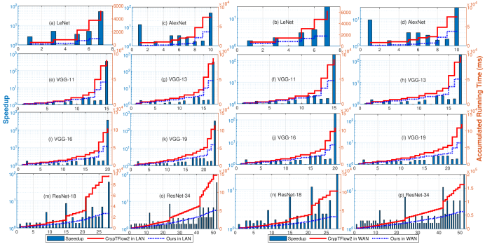
Next we test the runtime breakdown of each layer in our evaluated eight DL models as shown in Fig. 3, which allows us to have detailed observations. Specifically, the runtime for each layer includes all overhead for linear and nonlinear functions. Meanwhile, the layer index also includes the pooling, e.g., mean pooling. In LeNet, our protocol has noticeable speedup in each convolution layer (which includes Conv and ReLU) and the speedup is larger at last layer as our protocol only needs one HE multiplication while CrypTFlow2 involves a series of HE rotations. Similar observations are found in the last layer of other networks. In AlexNet, the large kernel width and height in the first layer, i.e., $f_{h}=f_{w}=11$, result in more rotations needed in CrypTFlow2 while the counterpart in our protocol is the same amount of multiplications, which is more efficient (see more details at Sec. 3.2). At the same time, the stride of 4 in the first layer involves 16 non-stride convolutions in CrypTFlow2 while our protocol benefits from the decreased data size to be transmitted and from the smaller computation overhead for strided convolution. As such our protocol gains a larger speedup. In VGG-11, VGG-13, VGG-16 and VGG-19, the speedup is larger in layer 11, 13, 15 and 17 (except the last layer) respectively. This is because large $c_{o}$ (i.e., the number of output channels) makes the gap between rotation and decryption more significant. As decryption is generally cheaper than multiplication, the speedup correspondingly increases. In ResNet-18 and ResNet-34, our protocol’s speedup is lager in layers 9, 15, 21 (except the last layer) with strided convolution, which is in line with the speedup for first layer in AlexNet. Similar observations are found in the WAN setting.

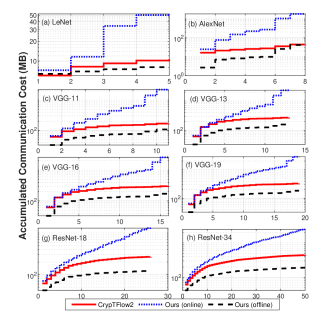
Finally, we show in Figure 4 the breakdown of communication overhead in each layer in our evaluated eight DL models. As demonstrated in Figure I, the gap in communication cost (i.e., the amount of data to be transmitted) between our protocol and CrypTFlow2 is proportional to the number of output channel $c_{o}$. As such we can see an increased difference between their communication cost as $c_{o}$ increases along the layers in all networks. But as we discussed earlier, despite the larger amount of data for communication, our protocol has noticeable overall performance gain (due to the reduced computation cost as analyzed in Sec. 3.2 and the lower communication cost before Conv) to offset the increased communication cost.

5 Conclusions

In this paper, we have challenged and broken the conventional compute-and-share logic for function output, and have proposed the share-in-the-middle logic, with which we have introduced the first joint linear and nonlinear computation across functions that features by 1) the PHE triplet for computing the intermediates of nonlinear function, with which the communication cost for multiplexing is eliminated; 2) the matrix encoding to calculate the intermediates of linear function, with which all rotations for summing is removed; and 3) the network adaptation to reassemble the model structure such that the recombined functions are able to take advantages of our proposed joint computation block as much as possible. The boosted efficiency of our protocol has been verified by the numerical complexity analysis and the experiments have also demonstrated up to 13$\times$ speedup for various functions used in the state-of-the-art models and up to $5\times$ speedup over mainstream neural networks compared with the state-of-the-art privacy-preserving frameworks. Furthermore, as the first one for share-in-the-middle computation, we have considered the joint computation between two adjacent functions while combing more functions forms an interesting work to explore more efficiency boost.

Qiao Zhang is an assistant professor at College of Computer Science, Chongqing University, China. Before that, She obtained her Ph.D. degree at Department of Electrical and Computer Engineering in Old Dominion University (21’). Her current research is about the privacy-preserved machine learning and she has published papers such as in NDSS, AsiaCCS, IJCAI, IEEE IoT Journal, IEEE TNSE.

Tao Xiang received the B.Eng., M.S. and Ph.D. degrees in computer science from Chongqing University, China, in 2003, 2005 and 2008, respectively. He is currently a Professor of the College of Computer Science at Chongqing University. Dr. Xiang’s research interests include multimedia security, cloud security, data privacy and cryptography. He has published over 90 papers on international journals and conferences. He also served as a referee for numerous international journals and conferences.

Chunsheng Xin is a Professor in the Department of Electrical and Computer Engineering, Old Dominion University. He received his Ph.D. in Computer Science and Engineering from the State University of New York at Buffalo in 2002. His interests include cybersecurity, machine learning, wireless communications and networking, cyber-physical systems, and Internet of Things. His research has been supported by almost 20 NSF and other federal grants, and results in more than 100 papers in leading journals and conferences, including three Best Paper Awards, as well as books, book chapters, and patent. He has served as Co-Editor-in-Chief/Associate Editors of multiple international journals, and symposium/track chairs of multiple international conferences including IEEE Globecom and ICCCN. He is a senior member of IEEE.

Biwen Chen received his Ph.D. degree from School of Computer, Wuhan University in 2020. He is currently an assistant professor of the School of Computer, Chongqing University, China. His main research interests include cryptography, information security and blockchain.

Hongyi Wu is a Professor and Department Head of Electrical and Computer Engineering at the University of Arizona. Between 2016-2022, He was a Batten Chair Professor and Director of the School of Cybersecurity at Old Dominion University (ODU). He was also a Professor in the Department of Electrical and Computer Engineering and held a joint appointment in the Department of Computer Science. Before joining ODU, He was an Alfred and Helen Lamson Professor at the Center for Advanced Computer Studies (CACS), the University of Louisiana at Lafayette. He received a B.S. degree in scientific instruments from Zhejiang University, Hangzhou, China, in 1996, and an M.S. degree in electrical engineering and a Ph.D. degree in computer science from the State University of New York (SUNY) at Buffalo in 2000 and 2002, respectively. His current research focuses on security and privacy in intelligent computing and communication systems. He chaired several conferences, including IEEE Infocom 2020. He served on the editorial board of several journals, such as IEEE Transactions on Computers, IEEE Transactions on Mobile Computing, IEEE Transactions on Parallel and Distributed Systems, and IEEE Internet of Things Journal. He received an NSF CAREER Award in 2004, UL Lafayette Distinguished Professor Award in 2011, and IEEE Percom Mark Weiser Best Paper Award in 2018. He is a Fellow of IEEE.

References

- [1] Y. LeCun, L. Bottou, Y. Bengio, and P. Haffner, “Gradient-based learning applied to document recognition,” Proceedings of the IEEE, vol. 86, no. 11, pp. 2278–2324, 1998.
- [2] A. Krizhevsky, I. Sutskever, and G. E. Hinton, “Imagenet classification with deep convolutional neural networks,” Advances in neural information processing systems, vol. 25, pp. 1097–1105, 2012.
- [3] K. Simonyan and A. Zisserman, “Very deep convolutional networks for large-scale image recognition,” arXiv preprint arXiv:1409.1556, 2014.
- [4] K. He, X. Zhang, S. Ren, and J. Sun, “Deep residual learning for image recognition,” in Proceedings of the IEEE conference on computer vision and pattern recognition, 2016, pp. 770–778.
- [5] C. Szegedy, W. Liu, Y. Jia, P. Sermanet, S. Reed, D. Anguelov, D. Erhan, V. Vanhoucke, and A. Rabinovich, “Going deeper with convolutions,” in Proceedings of the IEEE conference on computer vision and pattern recognition, 2015, pp. 1–9.
- [6] Y. Zhang, J. Qin, D. S. Park, W. Han, C.-C. Chiu, R. Pang, Q. V. Le, and Y. Wu, “Pushing the limits of semi-supervised learning for automatic speech recognition,” arXiv preprint arXiv:2010.10504, 2020.
- [7] S. Sohangir, D. Wang, A. Pomeranets, and T. M. Khoshgoftaar, “Big data: Deep learning for financial sentiment analysis,” Journal of Big Data, vol. 5, no. 1, pp. 1–25, 2018.
- [8] M. M. Najafabadi, F. Villanustre, T. M. Khoshgoftaar, N. Seliya, R. Wald, and E. Muharemagic, “Deep learning applications and challenges in big data analytics,” Journal of big data, vol. 2, no. 1, pp. 1–21, 2015.
- [9] H. C. Assistance, “Summary of the HIPAA privacy rule,” Office for Civil Rights, 2003.
- [10] M. Goddard, “The EU general data protection regulation (GDPR): European regulation that has a global impact,” International Journal of Market Research, vol. 59, no. 6, pp. 703–705, 2017.
- [11] R. Gilad-Bachrach, N. Dowlin, K. Laine, K. Lauter, M. Naehrig, and J. Wernsing, “Cryptonets: Applying neural networks to encrypted data with high throughput and accuracy,” in International Conference on Machine Learning. PMLR, 2016, pp. 201–210.
- [12] J. Liu, M. Juuti, Y. Lu, and N. Asokan, “Oblivious neural network predictions via minionn transformations,” in Proceedings of the 2017 ACM SIGSAC Conference on Computer and Communications Security, 2017, pp. 619–631.
- [13] C. Juvekar, V. Vaikuntanathan, and A. Chandrakasan, “GAZELLE: A low latency framework for secure neural network inference,” in 27th USENIX Security Symposium (USENIX Security 18), 2018, pp. 1651–1669.
- [14] P. Mohassel and Y. Zhang, “SecureML: A system for scalable privacy-preserving machine learning,” in 2017 IEEE Symposium on Security and Privacy (SP). IEEE, 2017, pp. 19–38.
- [15] M. S. Riazi, M. Samragh, H. Chen, K. Laine, K. Lauter, and F. Koushanfar, “XONN: Xnor-based oblivious deep neural network inference,” in 28th USENIX Security Symposium (USENIX Security 19), 2019, pp. 1501–1518.
- [16] P. Mishra, R. Lehmkuhl, A. Srinivasan, W. Zheng, and R. A. Popa, “DELPHI: A cryptographic inference service for neural networks,” in 29th USENIX Security Symposium (USENIX Security 20), 2020, pp. 2505–2522.
- [17] D. Rathee, M. Rathee, N. Kumar, N. Chandran, D. Gupta, A. Rastogi, and R. Sharma, “CrypTFlow2: Practical 2-party secure inference,” in Proceedings of the 2020 ACM SIGSAC Conference on Computer and Communications Security, 2020, pp. 325–342.
- [18] Q. Zhang, C. Xin, and H. Wu, “GALA: Greedy computation for linear algebra in privacy-preserved neural networks,” in ISOC Network and Distributed System Security Symposium, 2021.
- [19] A. Patra, T. Schneider, A. Suresh, and H. Yalame, “ABY2.0: Improved mixed-protocol secure two-party computation,” in 30th USENIX Security Symposium (USENIX Security 21), 2021.
- [20] S. Tan, B. Knott, Y. Tian, and D. J. Wu, “CRYPTGPU: Fast privacy-preserving machine learning on the gpu,” arXiv preprint arXiv:2104.10949, 2021.
- [21] M. S. Riazi, C. Weinert, O. Tkachenko, E. M. Songhori, T. Schneider, and F. Koushanfar, “Chameleon: A hybrid secure computation framework for machine learning applications,” in Proceedings of the 2018 on Asia Conference on Computer and Communications Security, 2018, pp. 707–721.
- [22] B. D. Rouhani, M. S. Riazi, and F. Koushanfar, “Deepsecure: Scalable provably-secure deep learning,” in Proceedings of the 55th Annual Design Automation Conference, 2018, pp. 1–6.
- [23] P. Mohassel and P. Rindal, “ABY3: A mixed protocol framework for machine learning,” in Proceedings of the 2018 ACM SIGSAC Conference on Computer and Communications Security, 2018, pp. 35–52.
- [24] F. Boemer, R. Cammarota, D. Demmler, T. Schneider, and H. Yalame, “MP2ML: a mixed-protocol machine learning framework for private inference,” in Proceedings of the 15th International Conference on Availability, Reliability and Security, 2020, pp. 1–10.
- [25] D. Demmler, T. Schneider, and M. Zohner, “ABY-a framework for efficient mixed-protocol secure two-party computation.” in NDSS, 2015.
- [26] Z. Brakerski, “Fully homomorphic encryption without modulus switching from classical gapsvp,” in Annual Cryptology Conference. Springer, 2012, pp. 868–886.
- [27] J. Fan and F. Vercauteren, “Somewhat practical fully homomorphic encryption.” IACR Cryptol. ePrint Arch., vol. 2012, p. 144, 2012.
- [28] J. H. Cheon, A. Kim, M. Kim, and Y. Song, “Homomorphic encryption for arithmetic of approximate numbers,” in International Conference on the Theory and Application of Cryptology and Information Security. Springer, 2017, pp. 409–437.
- [29] O. Goldreich, “Secure multi-party computation,” Manuscript. Preliminary version, vol. 78, 1998.
- [30] G. Brassard, C. Crépeau, and J.-M. Robert, “All-or-nothing disclosure of secrets,” in Conference on the Theory and Application of Cryptographic Techniques. Springer, 1986, pp. 234–238.
- [31] A. Shamir, “How to share a secret,” Communications of the ACM, vol. 22, no. 11, pp. 612–613, 1979.
- [32] M. Bellare, V. T. Hoang, and P. Rogaway, “Foundations of garbled circuits,” in Proceedings of the 2012 ACM conference on Computer and communications security, 2012, pp. 784–796.
- [33] A. C.-C. Yao, “How to generate and exchange secrets,” in 27th Annual Symposium on Foundations of Computer Science (sfcs 1986). IEEE, 1986, pp. 162–167.
- [34] “Alexa interface reference,” https://developer.amazon.com/en-US/docs/alexa/device-apis/alexa-response.html, 2021, accessed: 2021-06-06.
- [35] F. Mohammadzadeh, C. S. Nam, and E. Lobaton, “Prediction of physiological response over varying forecast lengths with a wearable health monitoring platform,” in 2018 40th Annual International Conference of the IEEE Engineering in Medicine and Biology Society (EMBC). IEEE, 2018, pp. 437–440.
- [36] S. U. Hussain, M. Javaheripi, M. Samragh, and F. Koushanfar, “Coinn: Crypto/ml codesign for oblivious inference via neural networks,” in Proceedings of the 2021 ACM SIGSAC Conference on Computer and Communications Security, 2021, pp. 3266–3281.
- [37] Z. Huang, W.-j. Lu, C. Hong, and J. Ding, “Cheetah: Lean and fast secure two-party deep neural network inference,” Cryptology ePrint Archive, 2022.
- [38] Y. Lindell, “How to simulate it–a tutorial on the simulation proof technique,” Tutorials on the Foundations of Cryptography, pp. 277–346, 2017.
- [39] R. Shokri, M. Stronati, C. Song, and V. Shmatikov, “Membership inference attacks against machine learning models,” in 2017 IEEE symposium on security and privacy (SP). IEEE, 2017, pp. 3–18.
- [40] F. Tramèr, F. Zhang, A. Juels, M. K. Reiter, and T. Ristenpart, “Stealing machine learning models via prediction APIs,” in 25th USENIX security symposium (USENIX Security 16), 2016, pp. 601–618.
- [41] M. Abadi, A. Chu, I. Goodfellow, H. B. McMahan, I. Mironov, K. Talwar, and L. Zhang, “Deep learning with differential privacy,” in Proceedings of the 2016 ACM SIGSAC conference on computer and communications security, 2016, pp. 308–318.
- [42] B. Jayaraman and D. Evans, “Evaluating differentially private machine learning in practice,” in 28th USENIX Security Symposium (USENIX Security 19), 2019, pp. 1895–1912.
- [43] V. Kolesnikov and R. Kumaresan, “Improved ot extension for transferring short secrets,” in Annual Cryptology Conference. Springer, 2013, pp. 54–70.
- [44] Y. Jia, E. Shelhamer, J. Donahue, S. Karayev, J. Long, R. Girshick, S. Guadarrama, and T. Darrell, “Caffe: Convolutional architecture for fast feature embedding,” in Proceedings of the 22nd ACM international conference on Multimedia, 2014, pp. 675–678.
- [45] S. Li, K. Xue, B. Zhu, C. Ding, X. Gao, D. Wei, and T. Wan, “Falcon: A fourier transform based approach for fast and secure convolutional neural network predictions,” in Proceedings of the IEEE/CVF Conference on Computer Vision and Pattern Recognition, 2020, pp. 8705–8714.
- [46] X. Liu, Y. Zheng, X. Yuan, and X. Yi, “Securely outsourcing neural network inference to the cloud with lightweight techniques,” IEEE Transactions on Dependable and Secure Computing, 2022.
- [47] “Execution order of relu and max-pooling,” https://github.com/tensorflow/tensorflow/issues/3180, 2022.
- [48] L. Deng, G. Li, S. Han, L. Shi, and Y. Xie, “Model compression and hardware acceleration for neural networks: A comprehensive survey,” Proceedings of the IEEE, vol. 108, no. 4, pp. 485–532, 2020.
- [49] Y. He, X. Zhang, and J. Sun, “Channel pruning for accelerating very deep neural networks,” in Proceedings of the IEEE international conference on computer vision, 2017, pp. 1389–1397.
- [50] S. Chen and Q. Zhao, “Shallowing deep networks: Layer-wise pruning based on feature representations,” IEEE transactions on pattern analysis and machine intelligence, vol. 41, no. 12, pp. 3048–3056, 2018.
- [51] “MNIST,” http://yann.lecun.com/exdb/mnist/, 2021.
- [52] “CIFAR10,” https://www.cs.toronto.edu/ kriz/cifar.html, 2021.
![[Uncaptioned image]](/html/2209.01637/assets/x5.jpg) |